


Rapeseed Area Extraction Based on Time-Series Dual-Polarization Radar Vegetation Indices

Abstract
:1. Introduction
2. Materials and Methods
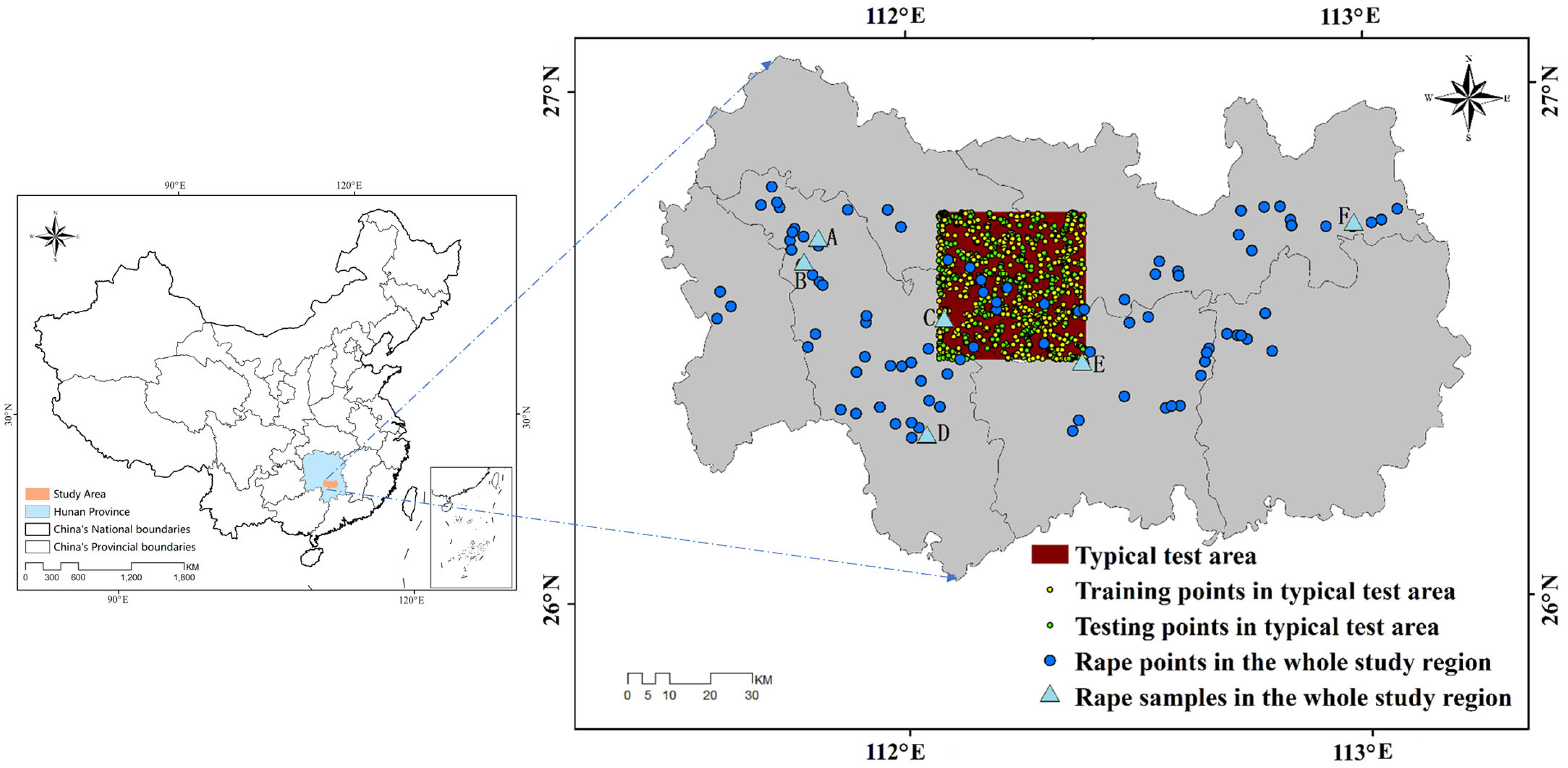
2.1. Study Region
2.2. Remote Sensing Data
2.3. Ground Sampling Points
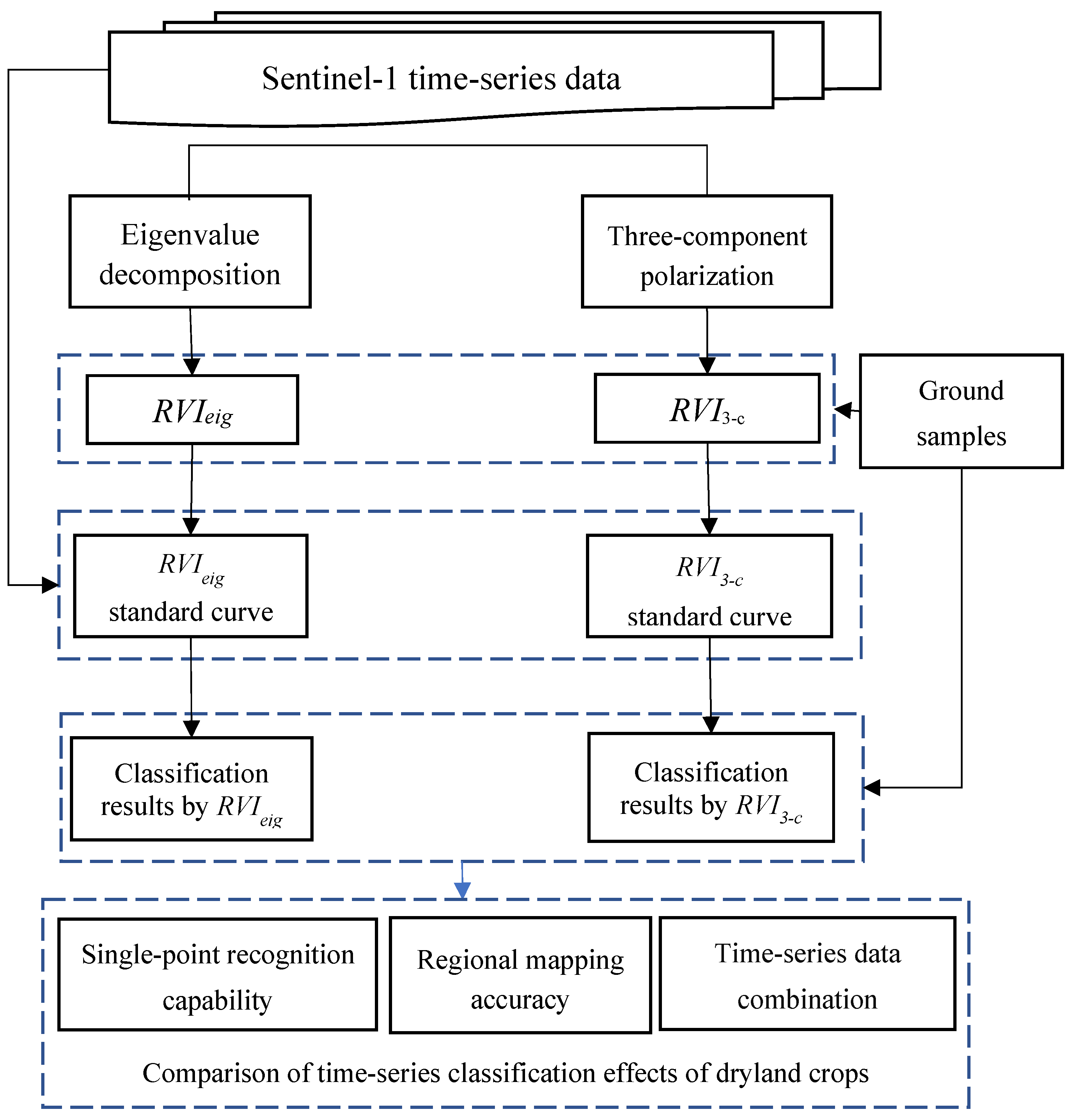
2.4. Methodology
- (1)
- Polarization decomposition:
- (2)
- Calculating the standard curves of the RVIs:
- (3)
- Time-series classification and class merging:
2.4.1. Eigenvalue Decomposition and RVI Calculation
2.4.2. Three-Component Decomposition and RVI Calculation
2.4.3. Comparative Indicators of the Extraction Effect
- (1)
- Single-point recognition capability:
- (2)
- Mapping accuracy:
- (3)
- Time-series data combination:
3. Results
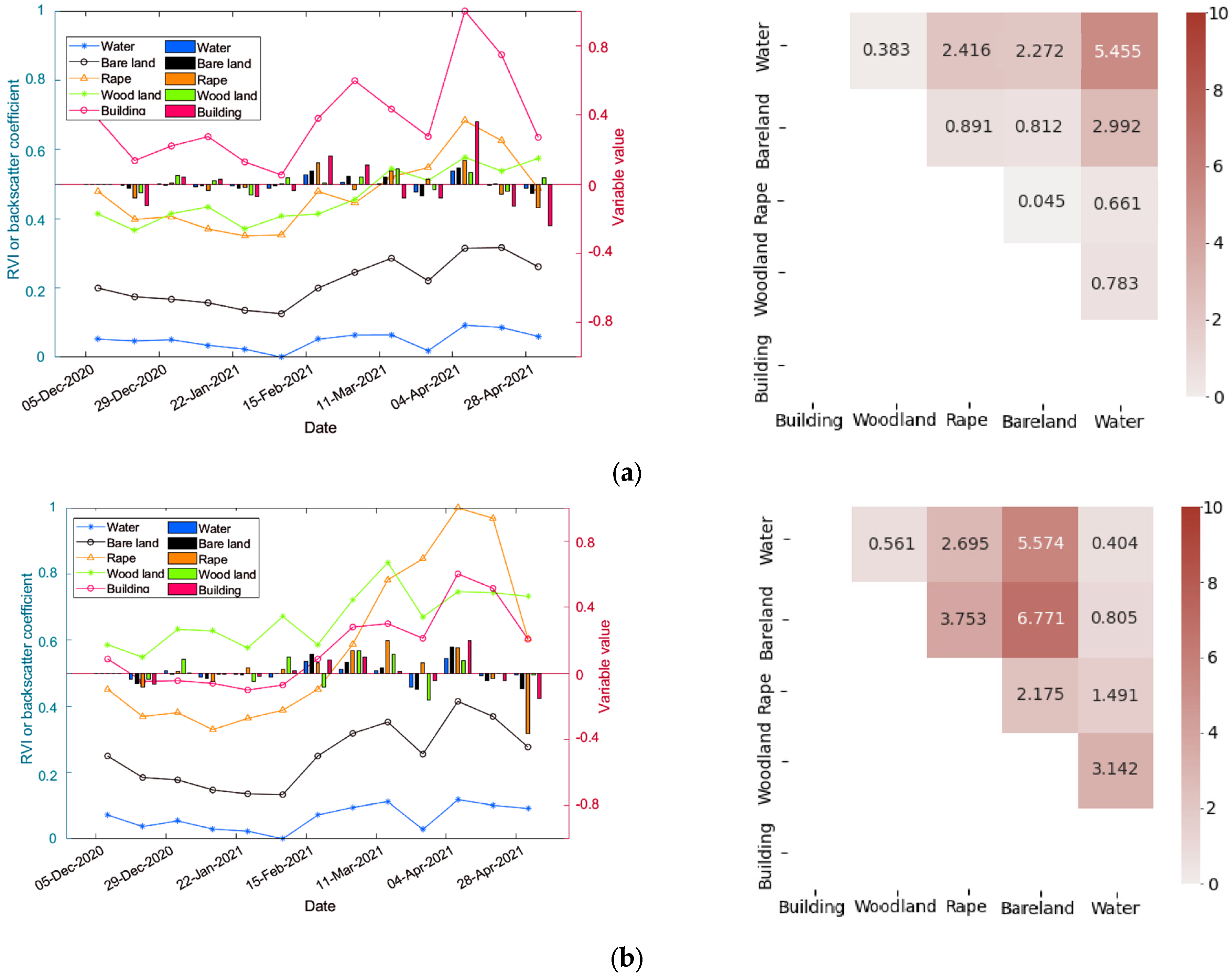
3.1. Single-Point Recognition Capability
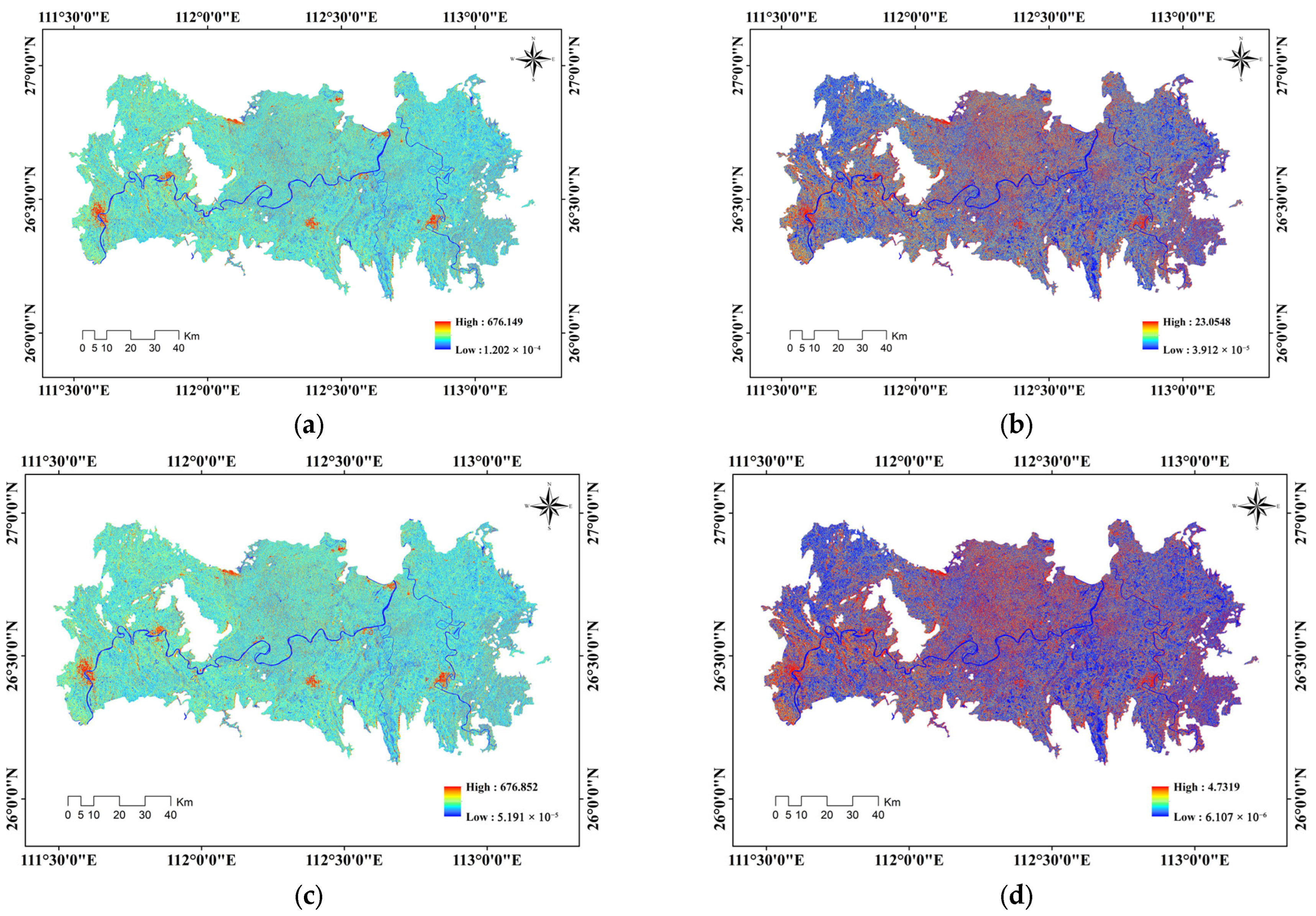
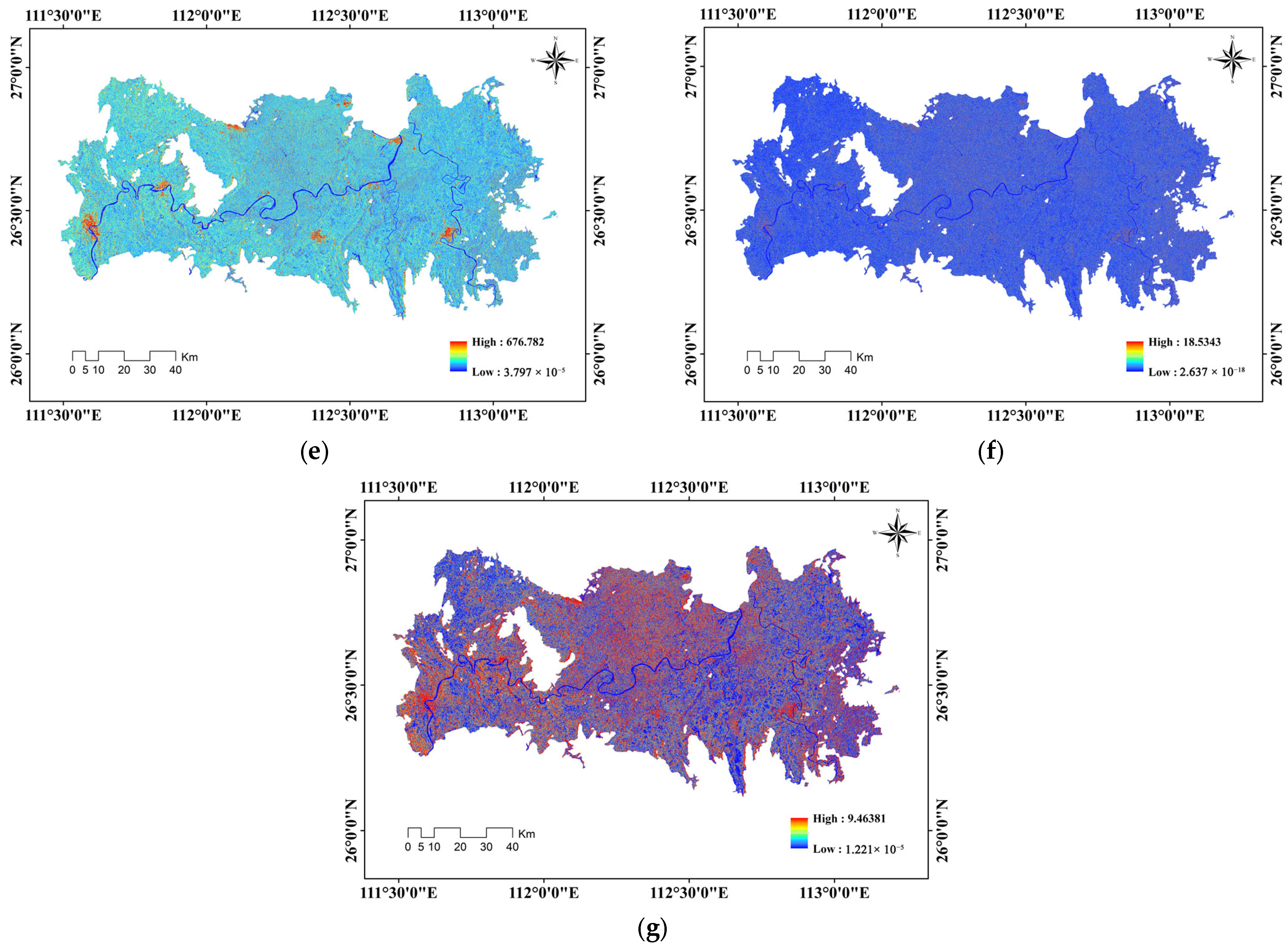
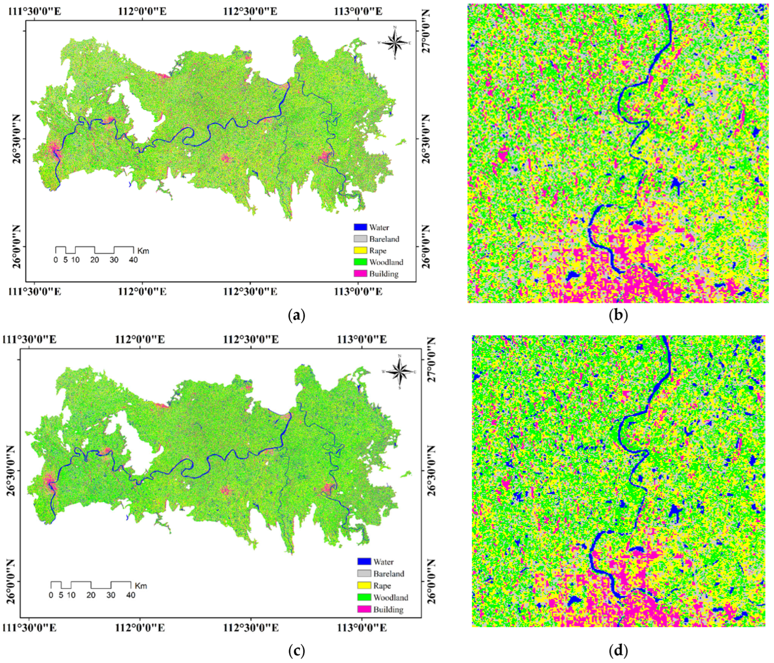
3.2. Mapping Accuracy
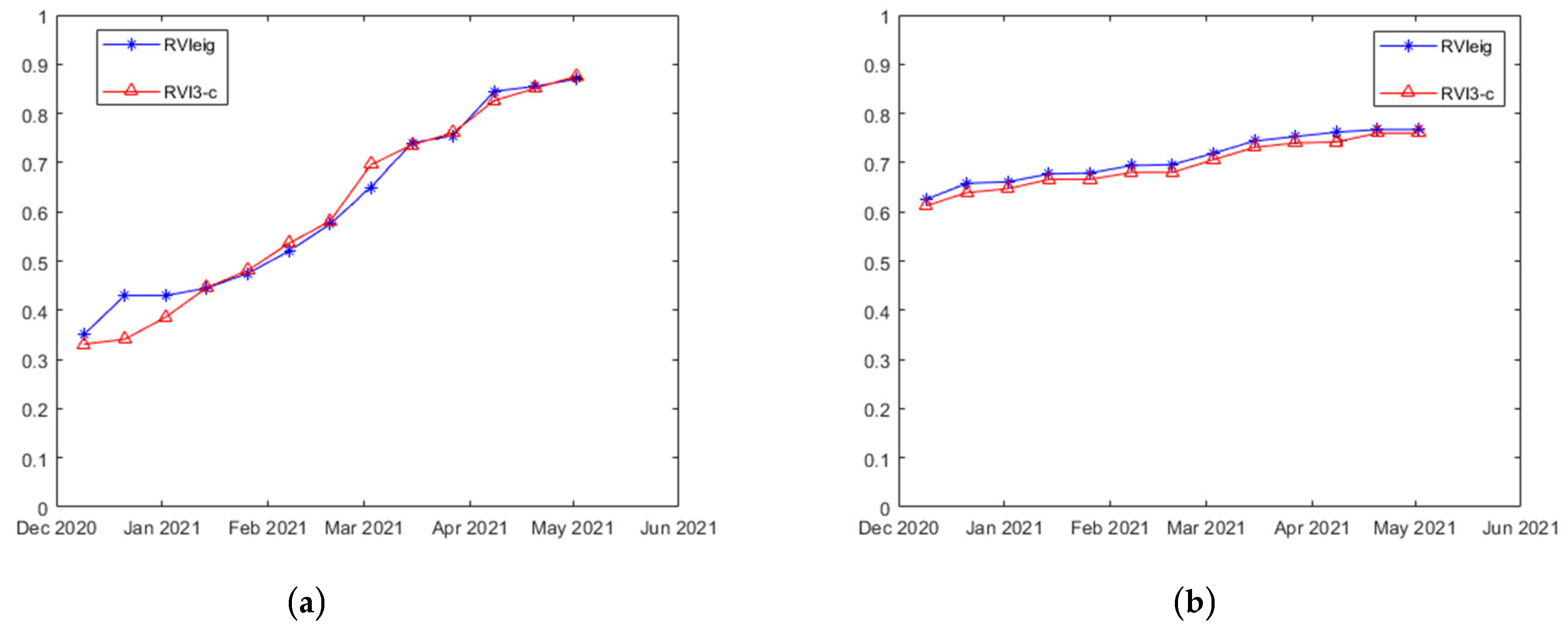
3.3. Time-Series Data Combination
4. Discussion
- (1)
- Applicability of polarization decomposition for dual-polarization data:
- (2)
- Comparison of rapeseed extraction applicability based on two typical polarization decompositions:
- (3)
- Limitations of this study, and future plans:
5. Conclusions
Author Contributions
Funding
Data Availability Statement
Conflicts of Interest
References
- Homayouni, S.; McNairn, H.; Hosseini, M.; Jiao, X.; Powers, J. Quad and compact multitemporal C-band PolSAR observations for crop characterization and monitoring. Int. J. Appl. Earth Obs. Geoinf. 2019, 74, 78–87. [Google Scholar] [CrossRef]
- Han, J.; Zhang, Z.; Luo, Y.; Cao, J.; Zhang, L.; Zhang, J.; Li, Z. The RapeseedMap10 database: Annual maps of Rapeseed at a spatial resolution of 10 m based on multisource data. Earth Syst. Sci. Data 2021, 13, 2857–2874. [Google Scholar] [CrossRef]
- Betbeder, J.; Fieuzal, R.; Philippets, Y.; Ferro-Famil, L.; Baup, F. Contribution of multitemporal polarimetric synthetic aperture radar data for monitoring winter wheat and Rapeseed crops. J. Appl. Remote Sens. 2016, 10, 026020. [Google Scholar] [CrossRef]
- Erten, E.; Lopez-Sanchez, J.M.; Yuzugullu, O.; Hajnsek, I. Retrieval of agricultural crop height from space: A comparison of SAR techniques. Remote Sens. Environ. 2016, 187, 130–144. [Google Scholar] [CrossRef]
- Canisius, F.; Shang, J.; Liu, J.; Huang, X.; Ma, B.; Jiao, X.; Geng, X.; Kovacs, J.M.; Walters, D. Tracking crop phenological development using multitemporal polarimetric Radarsat-2 data. Remote Sens. Environ. 2018, 210, 508–518. [Google Scholar] [CrossRef]
- Wang, H.; Magagi, R.; Goïta, K.; Trudel, M.; McNairn, H.; Powers, J. Crop phenology retrieval via polarimetric SAR decomposition and Random Forest algorithm. Remote Sens. Environ. 2019, 231, 111234. [Google Scholar] [CrossRef]
- Wali, E.; Tasumi, M.; Moriyama, M. Combination of linear regression lines to understand the response of Sentinel-1 dual polarization SAR data with crop phenology—Case study in Miyazaki, Japan. Remote Sens. 2020, 12, 189. [Google Scholar] [CrossRef]
- ESA. Sen4cap-Sentinels for Common Agriculture Policy. 2017. Available online: http://esa-sen4cap.org/ (accessed on 1 January 2022).
- Torres, R.; Snoeij, P.; Geudtner, D.; Bibby, D.; Davidson, M.; Attema, E.; Potin, P.; Rommen, B.; Floury, N.; Brown, M.; et al. GMES Sentinel-1 mission. Remote Sens. Environ. 2012, 120, 9–24. [Google Scholar] [CrossRef]
- Li, M.; Bijker, W. Vegetable classification in Indonesia using Dynamic Time Warping of Sentinel-1A dual polarization SAR time series. Int. J. Appl. Earth Obs. Geoinf. 2019, 78, 268–280. [Google Scholar] [CrossRef]
- Qu, Y.; Zhao, W.; Yuan, Z.; Chen, J. Crop mapping from sentinel-1 polarimetric time-series with a deep neural network. Remote Sens. 2020, 12, 2493. [Google Scholar] [CrossRef]
- Gella, G.W.; Bijker, W.; Belgiu, M. Mapping crop types in complex farming areas using SAR imagery with dynamic time warping. ISPRS J. Photogramm. Remote Sens. 2021, 175, 171–183. [Google Scholar] [CrossRef]
- Witharana, C.; Civco, D.L. Optimizing multiresolution segmentation scale using empirical methods: Exploring the sensitivity of the supervised discrepancy measure Euclidean distance 2 (ED2). ISPRS J. Photogramm. Remote Sens. 2014, 87, 108–121. [Google Scholar] [CrossRef]
- Deng, S.; Du, L.; Li, C.; Ding, J.; Liu, H. SAR automatic target recognition based on Euclidean distance restricted autoencoder. IEEE J. Sel. Top. Appl. Earth Obs. Remote Sens. 2017, 10, 3323–3333. [Google Scholar] [CrossRef]
- Csillik, O.; Belgiu, M.; Asner, G.P.; Kelly, M. Object-based time-constrained dynamic time warping classification of crops using Sentinel-2. Remote Sens. 2019, 11, 1257. [Google Scholar] [CrossRef]
- Moharana, S.; Kambhammettu BV, N.P.; Chintala, S.; Rani, A.S.; Avtar, R. Spatial distribution of inter- and intra-crop variability using time-weighted dynamic time warping analysis from Sentinel-1 datasets. Remote Sens. Appl. Soc. Environ. 2021, 24, 100630. [Google Scholar] [CrossRef]
- Li, H.; Wan, J.; Liu, S.; Sheng, H.; Xu, M. Wetland Vegetation Classification through Multi-Dimensional Feature Time Series Remote Sensing Images Using Mahalanobis Distance-Based Dynamic Time Warping. Remote Sens. 2022, 14, 501. [Google Scholar] [CrossRef]
- Wang, Z.; Wang, X.; Li, G.; Li, C. Robust cross-modal remote sensing image retrieval via maximal correlation augmentation. IEEE Trans. Geosci. Remote Sens. 2024, 62, 4705517. [Google Scholar] [CrossRef]
- Senin, P. Dynamic time warping algorithm review. Inf. Comput. Sci. Dep. Univ. Hawaii Manoa Honol. 2008, 855, 40. [Google Scholar]
- Guan, X.; Huang, C.; Liu, G.; Meng, X.; Liu, Q. Mapping rice cropping systems in Vietnam using an NDVI-based time-series similarity measurement based on DTW distance. Remote Sens. 2016, 8, 19. [Google Scholar] [CrossRef]
- Mondal, S.; Jeganathan, C. Mountain agriculture extraction from time-series MODIS NDVI using dynamic time warping technique. Int. J. Remote Sens. 2018, 39, 3679–3704. [Google Scholar] [CrossRef]
- Belgiu, M.; Zhou, Y.; Marshall, M.; Stein, A. Dynamic time warping for crops mapping. Int. Arch. Photogramm. Remote Sens. Spat. Inf. Sci. 2020, 43, 947–951. [Google Scholar] [CrossRef]
- Bazzi, H.; Baghdadi, N.; El Hajj, M.; Zribi, M.; Minh DH, T.; Ndikumana, E.; Courault, D.; Belhouchette, H. Mapping paddy rice using Sentinel-1 SAR time series in Camargue, France. Remote Sens. 2019, 11, 887. [Google Scholar] [CrossRef]
- Chang, L.; Chen, Y.T.; Wang, J.H.; Chang, Y.L. Rice-field mapping with Sentinel-1A SAR time-series data. Remote Sens. 2020, 13, 103. [Google Scholar] [CrossRef]
- Xu, L.; Zhang, H.; Wang, C.; Wei, S.; Zhang, B.; Wu, F.; Tang, Y. Paddy rice mapping in Thailand using time-series sentinel-1 data and deep learning model. Remote Sens. 2021, 13, 3994. [Google Scholar] [CrossRef]
- Vreugdenhil, M.; Wagner, W.; Bauer-Marschallinger, B.; Pfeil, I.; Teubner, I.; Rüdiger, C.; Strauss, P. Sensitivity of Sentinel-1 backscatter to vegetation dynamics: An Austrian case study. Remote Sens. 2018, 10, 1396. [Google Scholar] [CrossRef]
- d’Andrimont, R.; Taymans, M.; Lemoine, G.; Ceglar, A.; Yordanov, M.; van der Velde, M. Detecting flowering phenology in oil seed Rapeseed parcels with Sentinel-1 and-2 time series. Remote Sens. Environ. 2020, 239, 111660. [Google Scholar] [CrossRef]
- Meroni, M.; d’Andrimont, R.; Vrieling, A.; Fasbender, D.; Lemoine, G.; Rembold, F.; Seguinia, L.; Verhegghen, A. Comparing land surface phenology of major European crops as derived from SAR and multispectral data of Sentinel-1 and-2. Remote Sens. Environ. 2021, 253, 112232. [Google Scholar] [CrossRef]
- Qi, Z.; Yeh, A.G.O.; Li, X.; Lin, Z. A novel algorithm for land use and land cover classification using RADARSAT-2 polarimetric SAR data. Remote Sens. Environ. 2012, 118, 21–39. [Google Scholar] [CrossRef]
- Chauhan, S.; Darvishzadeh, R.; Boschetti, M.; Nelson, A. Estimation of crop angle of inclination for lodged wheat using multi-sensor SAR data. Remote Sens. Environ. 2020, 236, 111488. [Google Scholar] [CrossRef]
- Bhogapurapu, N.; Dey, S.; Bhattacharya, A.; Mandal, D.; Lopez-Sanchez, J.M.; McNairn, H.; López-Martínez, C.; Rao, Y.S. Dual-polarimetric descriptors from Sentinel-1 GRD SAR data for crop growth assessment. ISPRS J. Photogramm. Remote Sens. 2021, 178, 20–35. [Google Scholar] [CrossRef]
- Xu, S.; Zhu, X.; Cao, R.; Chen, J.; Ding, X. Automatic SAR-based rapeseed mapping in all terrain and weather conditions using dual-aspect Sentinel-1 time series. Remote Sens. Environ. 2025, 318, 114567. [Google Scholar] [CrossRef]
- Wang, M.; Wang, L.; Guo, Y.; Cui, Y.; Liu, J.; Chen, L.; Wang, T.; Li, H. A Comprehensive Evaluation of Dual-Polarimetric Sentinel-1 SAR Data for Monitoring Key Phenological Stages of Winter Wheat. Remote Sens. 2024, 16, 1659. [Google Scholar] [CrossRef]
- Ji, K.; Wu, Y. Scattering mechanism extraction by a modified cloude-pottier decomposition for dual polarization SAR. Remote Sens. 2015, 7, 7447–7470. [Google Scholar] [CrossRef]
- Guo, J.; Wei, P.L.; Liu, J.; Jin, B.; Su, B.F.; Zhou, Z.S. Crop classification based on differential characteristics of h/alpha scattering parameters for multitemporal quad-and dual-polarization SAR images. IEEE Trans. Geosci. Remote Sens. 2018, 56, 6111–6123. [Google Scholar] [CrossRef]
- Nie, C.; Long, D.G. A C-band scatterometer simultaneous wind/rain retrieval method. IEEE Trans. Geosci. Remote Sens. 2008, 46, 3618–3631. [Google Scholar] [CrossRef]
- Mandal, D.; Ratha, D.; Bhattacharya, A.; Kumar, V.; McNairn, H.; Rao, Y.; Frery, A. A radar vegetation index for crop monitoring using compact polarimetric SAR data. IEEE Trans. Geosci. Remote Sens. 2020, 58, 6321–6335. [Google Scholar] [CrossRef]
- Mandal, D.; Kumar, V.; Ratha, D.; Dey, S.; Bhattacharya, A.; Lopez-Sanchez, J.M.; McNairn, H.; Rao, Y.S. Dual polarimetric radar vegetation index for crop growth monitoring using sentinel-1 SAR data. Remote Sens. Environ. 2020, 247, 111954. [Google Scholar] [CrossRef]
- Guo, R.; Liu, Y.B.; Wu, Y.H.; Zhang, S.X.; Xing, M.D.; He, W. Applying H/α decomposition to compact polarimetric SAR. IET Radar Sonar Navig. 2012, 6, 61–70. [Google Scholar] [CrossRef]
- Han, K.; Jiang, M.; Wang, M.; Liu, G. Compact polarimetric SAR interferometry target decomposition with the Freeman–Durden method. IEEE J. Sel. Top. Appl. Earth Obs. Remote Sens. 2018, 11, 2847–2861. [Google Scholar] [CrossRef]
- Jalilibal, Z.; Amiri, A.; Castagliola, P.; Khoo, M.B. Monitoring the coefficient of variation: A literature review. Comput. Ind. Eng. 2021, 161, 107600. [Google Scholar] [CrossRef]
- Yacouby, R.; Axman, D. Probabilistic extension of precision, recall, and f1 score for more thorough evaluation of classification models. In Proceedings of the First Workshop on Evaluation and Comparison of NLP Systems, Online, 20 November 2020; pp. 79–91. [Google Scholar]
- Belgiu, M.; Drăguţ, L. Random forest in remote sensing: A review of applications and future directions. ISPRS J. Photogramm. Remote Sens. 2016, 114, 24–31. [Google Scholar] [CrossRef]
- Tulbure, M.G.; Broich, M.; Stehman, S.V.; Kommareddy, A. Surface water extent dynamics from three decades of seasonally continuous Landsat time series at subcontinental scale in a semiarid region. Remote Sens. Environ. 2016, 178, 142–157. [Google Scholar] [CrossRef]
- Wu, D.; Zeng, G.; Meng, L.; Zhou, W.; Li, L. Gini coefficient-based task allocation for multirobot systems with limited energy resources. IEEE/CAA J. Autom. Sin. 2017, 5, 155–168. [Google Scholar] [CrossRef]
- Pan, B.; Zheng, Y.; Shen, R.; Ye, T.; Zhao, W.; Dong, J.; Ma, H.; Yuan, W. High resolution distribution dataset of double-season paddy rice in China. Remote Sens. 2021, 13, 4609. [Google Scholar] [CrossRef]


| Phenology | Seedling | Bolting | Flowering | Silique | Maturity |
|---|---|---|---|---|---|
| Date | Oct. to Dec. | Early Jan. to mid-Feb. of the subsequent year | Mid-Feb. to Late Mar. of the subsequent year | Late Mar. to Late Apr. of the subsequent year | Late Apr. of the subsequent year |
| Picture |  | 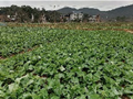 | 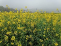 | 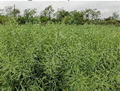 | 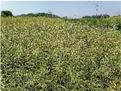 |
| No. | Satellite | Date | Absolute Track Number | Relative Track Number | Rapeseed Growth Stage | Precipitation 08-08 h (mm) | Cloud Coverage of Sentinel-2 |
|---|---|---|---|---|---|---|---|
| 1 | 1A | 20201209 | 035608 | 11 | Seedling | 0.0 | 100.00% |
| 2 | 1A | 20201221 | 035783 | 11 | Seedling | 0.0 | 100.00% |
| 3 | 1A | 20210102 | 035958 | 11 | Bolting | 0.0 | 0.38% |
| 4 | 1A | 20210114 | 036133 | 11 | Bolting | 0.0 | 2.33% |
| 5 | 1A | 20210126 | 036308 | 11 | Bolting | 0.0 | 100.00% |
| 6 | 1A | 20210207 | 036483 | 11 | Flowering | 0.0 | 1.17% |
| 7 | 1A | 20210219 | 036658 | 11 | Flowering | 0.0 | 38.25% |
| 8 | 1A | 20210303 | 036833 | 11 | Flowering | 4.4 | 100.00% |
| 9 | 1A | 20210315 | 037008 | 11 | Flowering | 0.0 | 99.99% |
| 10 | 1A | 20210327 | 037183 | 11 | Silique | 0.0 | 62.65% |
| 11 | 1A | 20210408 | 037358 | 11 | Silique | 3.4 | 99.99% |
| 12 | 1A | 20210420 | 037533 | 11 | Maturity | 0.0 | 99.25% |
| 13 | 1A | 20210502 | 037708 | 11 | Maturity | 0.2 | 99.89% |
| No. | Distance from the Center of Typical Test Area (km) | Thumbnail | No. | Distance from the Center of Typical Test Area (km) | Thumbnail |
|---|---|---|---|---|---|
| Sample A | 48.48 |  | Sample B | 46.48 | 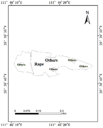 |
| Sample C | 16.08 |  | Sample D | 36.09 | 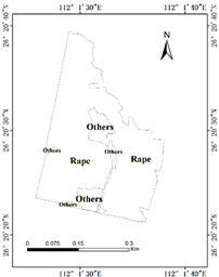 |
| Sample E | 21.72 | 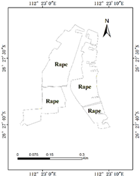 | Sample F | 77.31 | 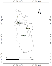 |
| Whole Image | Sample A | Sample B | Sample C | Sample D | Sample E | Sample F | |
|---|---|---|---|---|---|---|---|
| VV | 2.38 | 24.32 | 24.85 | 1.15 | 26.75 | 26.16 | 33.79 |
| VH | 0.88 | 0.36 | 0.37 | 0.41 | 0.36 | 0.31 | 0.33 |
| 2.36 | 24.55 | 24.59 | 1.16 | 26.73 | 25.53 | 33.59 | |
| 0.77 | 0.35 | 0.36 | 0.34 | 0.36 | 0.31 | 0.33 | |
| 0.03 | 0.26 | 0.39 | 1.44 | 0.35 | 0.39 | 0.44 | |
| 5.13 | 0.16 | 1.46 | 1.54 | 0.14 | 1.44 | 1.54 | |
| 0.74 | 0.36 | 0.39 | 0.42 | 0.44 | 0.33 | 0.33 |
| Points in Typical Test Area | Points in Whole Study Region | Sample A | Sample B | Sample C | Sample D | Sample E | Sample F | Total | ||
|---|---|---|---|---|---|---|---|---|---|---|
| TP | 73 | 67 | 169 | 82 | 64 | 298 | 204 | 216 | 1173 | |
| TN | 362 | 0 | 4 | 7 | 3 | 15 | 0 | 24 | 415 | |
| FP | 27 | 27 | 40 | 72 | 51 | 97 | 78 | 215 | 607 | |
| FN | 38 | 0 | 2 | 9 | 2 | 17 | 0 | 6 | 74 | |
| OA(%) | 87.00 | 71.28 | 80.47 | 52.35 | 55.83 | 73.30 | 72.34 | 52.06 | 69.99 | |
| P(%) | 73.00 | 71.28 | 80.86 | 53.25 | 55.65 | 75.44 | 72.34 | 50.12 | 65.90 | |
| R(%) | 65.77 | - | 98.83 | 90.11 | 96.97 | 94.60 | - | 97.30 | 94.07 | |
| F-1(%) | 69.19 | 83.23 | 88.95 | 66.94 | 70.72 | 83.94 | 83.95 | 66.16 | 77.50 | |
| TP | 73 | 67 | 180 | 87 | 66 | 295 | 204 | 281 | 1253 | |
| TN | 365 | 0 | 4 | 5 | 4 | 27 | 0 | 24 | 429 | |
| FP | 27 | 27 | 30 | 69 | 48 | 88 | 78 | 146 | 513 | |
| FN | 35 | 0 | 1 | 9 | 2 | 17 | 0 | 10 | 74 | |
| OA(%) | 87.60 | 71.28 | 85.58 | 54.12 | 58.33 | 75.41 | 72.34 | 66.16 | 74.13 | |
| P(%) | 73.00 | 71.28 | 85.71 | 55.77 | 57.89 | 77.02 | 72.34 | 65.81 | 70.95 | |
| R(%) | 67.59 | - | 99.45 | 90.63 | 97.06 | 94.55 | - | 96.56 | 94.42 | |
| F-1(%) | 70.19 | 83.23 | 92.07 | 69.05 | 72.53 | 84.89 | 83.95 | 78.27 | 81.02 |
Disclaimer/Publisher’s Note: The statements, opinions and data contained in all publications are solely those of the individual author(s) and contributor(s) and not of MDPI and/or the editor(s). MDPI and/or the editor(s) disclaim responsibility for any injury to people or property resulting from any ideas, methods, instructions or products referred to in the content. |
© 2025 by the authors. Licensee MDPI, Basel, Switzerland. This article is an open access article distributed under the terms and conditions of the Creative Commons Attribution (CC BY) license (https://creativecommons.org/licenses/by/4.0/).
Share and Cite
Zhu, Y.; Cao, H.; Wu, S.; Guo, Y.; Song, Q. Rapeseed Area Extraction Based on Time-Series Dual-Polarization Radar Vegetation Indices. Remote Sens. 2025, 17, 1479. https://doi.org/10.3390/rs17081479
Zhu Y, Cao H, Wu S, Guo Y, Song Q. Rapeseed Area Extraction Based on Time-Series Dual-Polarization Radar Vegetation Indices. Remote Sensing. 2025; 17(8):1479. https://doi.org/10.3390/rs17081479
Chicago/Turabian StyleZhu, Yiqing, Hong Cao, Shangrong Wu, Yongli Guo, and Qian Song. 2025. "Rapeseed Area Extraction Based on Time-Series Dual-Polarization Radar Vegetation Indices" Remote Sensing 17, no. 8: 1479. https://doi.org/10.3390/rs17081479
APA StyleZhu, Y., Cao, H., Wu, S., Guo, Y., & Song, Q. (2025). Rapeseed Area Extraction Based on Time-Series Dual-Polarization Radar Vegetation Indices. Remote Sensing, 17(8), 1479. https://doi.org/10.3390/rs17081479