Multi-Year Global Oscillations in GNSS Deformation and Surface Loading Contributions

Abstract

Recent studies have identified a near six-year oscillation (SYO) in Global Navigation Satellite Systems (GNSS) surface displacements, with a degree 2, order 2 spherical harmonic (SH) pattern and retrograde motion. The cause is uncertain, with proposals ranging from deep Earth to near-surface sources. This study investigates the SYO and possible causes from surface loading. Considering the irregular spatiotemporal distribution of GNSS data and the variety of contributors to surface displacements, we used synthetic experiments to identify optimal techniques for estimating low degree SH patterns. We confirm a reported retrograde SH degree 2, order 2 displacement using GNSS data from the same 35 stations used in a previous study for the 1995–2015 period. We also note that its amplitude diminished when the time span of observations was extended to 2023, and the retrograde dominance became less significant using a larger 271-station set. Surface loading estimates showed that terrestrial water storage (TWS) loads contributed much more to the GNSS degree 2, order 2 SYO, than atmospheric and oceanic loads, but TWS load estimates were highly variable. Four TWS sources—European Centre for Medium-Range Weather Forecasts Reanalysis 5 (ERA5), Modern-Era Retrospective analysis for Research and Applications (MERRA), Global Land Data Assimilation System (GLDAS), and Gravity Recovery and Climate Experiment (GRACE/GRACE Follow-On)—yielded a wide range (24% to 93%) of predicted TWS contributions with GRACE/GRACE Follow-On being the largest. This suggests that TWS may be largely responsible for SYO variations in GNSS observations. Variations in SYO GNSS amplitudes in the extended period (1995–2023) were also consistent with near surface sources.

1. Introduction

A ~six-year oscillation (SYO) has been detected throughout the Earth system, including length of day changes (ΔLOD) [1,2,3], polar motion [4], magnetic field [5], gravity field [6,7], surface deformation [8,9], and the climate system [10,11,12]. The authors of [12] provided a comprehensive review and discussion of the difficulties in identifying precisely the period(s) of fluctuations in varied geophysical properties, due to limitations imposed by data length. The authors of [13] proposed several scenarios to explore the causes of SYO from Earth’s deep interior to the climate system, but its origin remains uncertain. The SYO in ΔLOD has been attributed to the deep Earth [4,14,15,16,17], with various proposed physical causes, including Mantle-Inner-Core Gravitational coupling (MICG) and torsional modes in the outer core. For the SYO in surface deformation, the authors of [8,9] also proposed deep Earth sources, but other work [18] indicated that surface displacements resulting from core processes would be too small to be detected in Global Navigation Satellite Systems (GNSS) observations. The authors of [19] identified the SYO in GNSS interannual signals in reginal surface loading studies and highlighted the complexity of its cause. Their findings revealed inconsistencies in the amplitude and phase agreements between GNSS and environmental loadings. A near SYO in surface deformation, gravity field, and other quantities suggests the importance of climate sources [20]. Additionally, the authors of [21] found SYO variations at specific GNSS stations, which would be associated with regional climate effects.

Here, we use the term SYO to imply variations over periods near but not precisely lasting six years. We focus on strategies for estimating SYO pro- and retrograde variations having a SH degree 2, order 2 (abbreviated [2, 2]) pattern in GNSS (here, only Global Positioning System (GPS)) surface deformation, as reported in [8], and examine geophysical contributions from surface loading. Because deep Earth sources at higher SH degrees would have diminished surface effects [22,23], [2, 2] variations are a good candidate for study. The authors of [9] found evidence of a SYO in a stack (average) of 12 years of GPS vertical displacements at 523 stations, although averaging over all longitudes would likely attenuate a [2, 2] pattern.

The 38 GPS stations used in [8] were very unevenly distributed, with only four in the Southern Hemisphere. This imbalance may have allowed local signals, such as the ~six-year periodic signal associated with land hydrology in California [24], to introduce aliasing in the [2, 2] estimate. Therefore, the first topic of our study was identifying an effective strategy for the estimation of a [2, 2] pattern from available data. Our second topic was understanding the contamination, uncertainty, and deformation associated with observational noise and surface loading from atmospheric, oceanic, and land hydrological (terrestrial water storage or TWS) sources. Quantification of surface loading sources were expected to help identify cause(s) of SYO behavior which have varied explanations, as mentioned above. We examined various loading contributions from model estimates and satellite gravimetry observations.

2. Materials and Methods

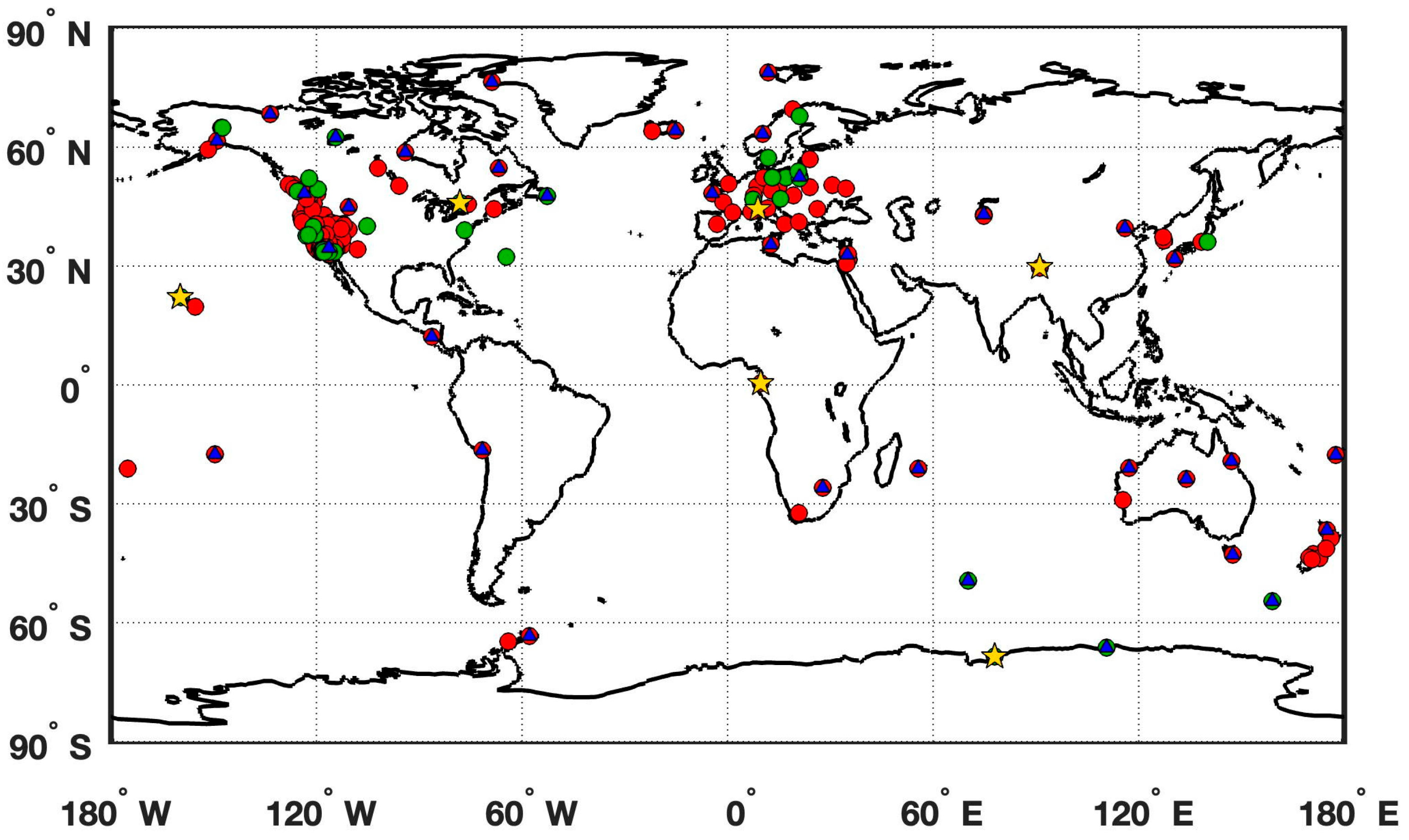
2.1. GPS Data

The GPS vertical displacement time series used in this study are from NASA’s Jet Propulsion Laboratory (JPL), which provides data from more than 2800 stations [25]. Two station sets were selected, one being the same used in [8] comprising 38 stations, covering the period from January 1995 to April 2015, and the other comprising 271 stations spanning April 2002 to May 2023. For both station sets, we applied the same data selection criteria as in [8], ensuring data gaps were below 180 days. Figure 1 shows the locations of the 38 and 271 station sets. A list of stations used in this study is shown in the Supporting Information (Table S1). Breaks and jumps caused by equipment changes and earthquakes, as well as annual and semi-annual terms, have been removed using JPL estimates. A least square fit (LSQ) linear trend was removed prior to spectral analysis. Figure 2 shows the monthly GPS vertical displacements (black curves) for the ALGO (North America), DAV1 (Antarctica), GENO (Southern Europe), KOKB (Central Pacific), LHAZ (Central Asia), and NKLG (West Africa) stations, as examples. These example stations are indicated by gold stars in Figure 1.

2.2. Loading Data

The School and Observatory of Earth Sciences (EOST) loading service (http://loading.u-strasbg.fr/index.php) provides estimates of surface deformations from various climate sources as both Stokes coefficients and station displacements [26,27]. We used EOST center-of-figure station displacements in this study. EOST estimates atmospheric loads from two surface pressure data sources, the European Centre for Medium-Range Weather Forecasts Reanalysis 5 (ERA5) and the Modern-Era Retrospective analysis for Research and Applications, Version 2 (MERRA-2). EOST non-tidal oceanic loading is estimated from ocean bottom pressure (OBP) data provided by the Circulation and Climate of the Ocean, Phase II (ECCO2). Because atmospheric and oceanic contributions are largely anti-correlated over the oceans due to the inverted barometer (IB) response of the oceans, we separated continental and oceanic loads to clarify their individual contributions. The continental component was calculated from surface pressure data over land only. The ocean component was calculated directly from OBP containing both atmospheric and oceanic loads.

EOST terrestrial water storage (TWS) loading was estimated from soil moisture, snow, and canopy water data from three sources, ERA5, MERRA-2, and the Global Land Data Assimilation System (GLDAS). In addition to these EOST TWS estimates, Gravity Recovery and Climate Experiment (GRACE) and GRACE Follow-On (GRACE-FO) gravity data were available to estimate TWS loading displacement. We used the University of Texas at Austin Center for Space Research (UTCSR) Release 6.2 (RL06.2) $0.25°\times 0.25°$ mascon solutions [28,29], which have been supplemented at low SH degrees using satellite laser ranging data (${\mathrm{C}}_{20},$${\mathrm{C}}_{30}$) with estimated degree-1 (${\mathrm{C}}_{10},$${\mathrm{C}}_{11},$${\mathrm{S}}_{11}$) coefficients, corrections for glacial isostatic adjustment (GIA), and GAD fields (equivalent to OBP over the oceans). We subtracted GAD gridded fields so that the residual equivalent water thickness (EWT) over land would represent TWS loading. The approximately one-year gap between GRACE and GRACE-FO, along with smaller gaps within the GRACE and GRACE-FO period, was addressed by first removing the average seasonal components, linearly interpolating the residual time series, and then restoring the seasonal components. The GRACE/GRACE-FO estimates of TWS vertical loading displacements were calculated by convolution of EWT with a Green’s function for the Preliminary Reference Earth Model [30,31]. The Green’s function, in Figure S1, shows that displacement dropped rapidly away from the load. For example, the vertical displacement of a 10 km disc load fell to about 10% of its peak value at about 30 km from the load center.

For our initial calculations, we selected load estimates from ERA5, ECCO2, and ERA5 models for atmosphere, OBP, and TWS loads, respectively. Their cumulative vertical loading displacements at the six example stations are shown by red curves in Figure 2. Subsequently, we examined other climate model and GRACE/GRACE-FO estimates. In fact, the differences among atmospheric model estimates were small (Figure S2 shows this for the six example station time series), whereas Figure 3 shows relatively larger differences among TWS load estimates from hydrological models and GRACE/GRACE-FO data. The large differences at specific stations were likely due to limited data coverage in certain regions (e.g., the absence of modeled data over Antarctica at DAV1) or differences in land–ocean mask definitions among models, which may have led to inconsistencies in TWS estimates near coastal stations (e.g., NKLG).

2.3. Methods

Surface deformation $V\left(\theta ,\varphi \right)$ at colatitude $\theta$ and longitude $\varphi$ can be expressed in a SH expansion:

$$V\left(\theta ,\varphi \right)=\sum _{l=0}^N\sum _{m=0}^l{P}_{lm}\left(\cos \theta \right)\left(C_{lm}\cos m\varphi +S_{lm}\sin m\varphi \right)$$

(1)

where $P_{lm}\left(\cos \theta \right)$ are normalized Legendre functions of degree l and order m, and $C_{lm}$, and $S_{lm}$ are real-valued SH coefficients. N is the maximum expansion degree. Coefficients $C_{lm}$ and $S_{lm}$ were estimated via LSQ from GPS surface displacements (Equation (2)):

$$\left[\begin{array}{c}C\\ S\end{array}\right]={\left(Y^{T}WY\right)}^{-1}{Y}^{T}WV$$

(2)

where Y represents the degree and order summation of $P_{lm}\left(\cos \theta \right)$ multiplied by $\cos m\varphi$ or $\sin m\varphi$, W is a weight applied to vertical displacement data, and C, S, and V represent $C_{lm}$, $S_{lm}$, and $V\left(\theta ,\varphi \right)$, respectively. We omit the summation symbol for conciseness. The total number of coefficients for a specific degree l was 2l + 1, so displacements at a minimum of five GPS stations were needed to estimate degree 2 coefficients, but the actual number of stations would be larger, so data quality and geographical distribution needed to be considered when interpreting estimates.

To replicate and extend the results of [8], we estimated SH [2, 2] coefficients ${\mathrm{C}}_{22}$ and ${\mathrm{S}}_{22}$ using LSQ fits to vertical displacements and then expressed time series of coefficients in the complex form ${\mathrm{C}}_{22}+i{\mathrm{S}}_{22}$ to allow pro- and retrograde separation. The next section examines various approaches to LSQ estimation considering the irregular spatial sampling of the station sets. Periodogram spectra from the Discrete Fourier Transform (DFT) of ${\mathrm{C}}_{22}+i{\mathrm{S}}_{22}$ time series separated positive and negative frequencies, corresponding to pro- and retrograde variations, respectively. In addition, real-valued Morlet wavelet spectral analysis [32,33,34] was used to examine time-varying spectra of pro- and retrograde components:

$$F\left(a,b\right)={\displaystyle \frac{1}{\sqrt{a}}}{\int }_{-\infty }^{\infty }f\left(t\right)W\left({\displaystyle \frac{t-b}{a}}\right)dt$$

(3)

$$W\left({\displaystyle \frac{t-b}{a}}\right)={\displaystyle \frac{1}{\sqrt{2a\pi }}}{e}^{-{\displaystyle \frac{{\left(t-b\right)}^2}{2a^2}}}\cos \left(\sqrt{{\displaystyle \frac{2}{\ln 2}}}\pi ·{\displaystyle \frac{t-b}{a}}\right)$$

(4)

where $F\left(a,b\right)$ is the amplitude at frequency/period $a$ and time $b$, $f\left(t\right)$ is the time series, and $W\left({\displaystyle \frac{t-b}{a}}\right)$ represents the Morlet basis wavelet.

3. Results

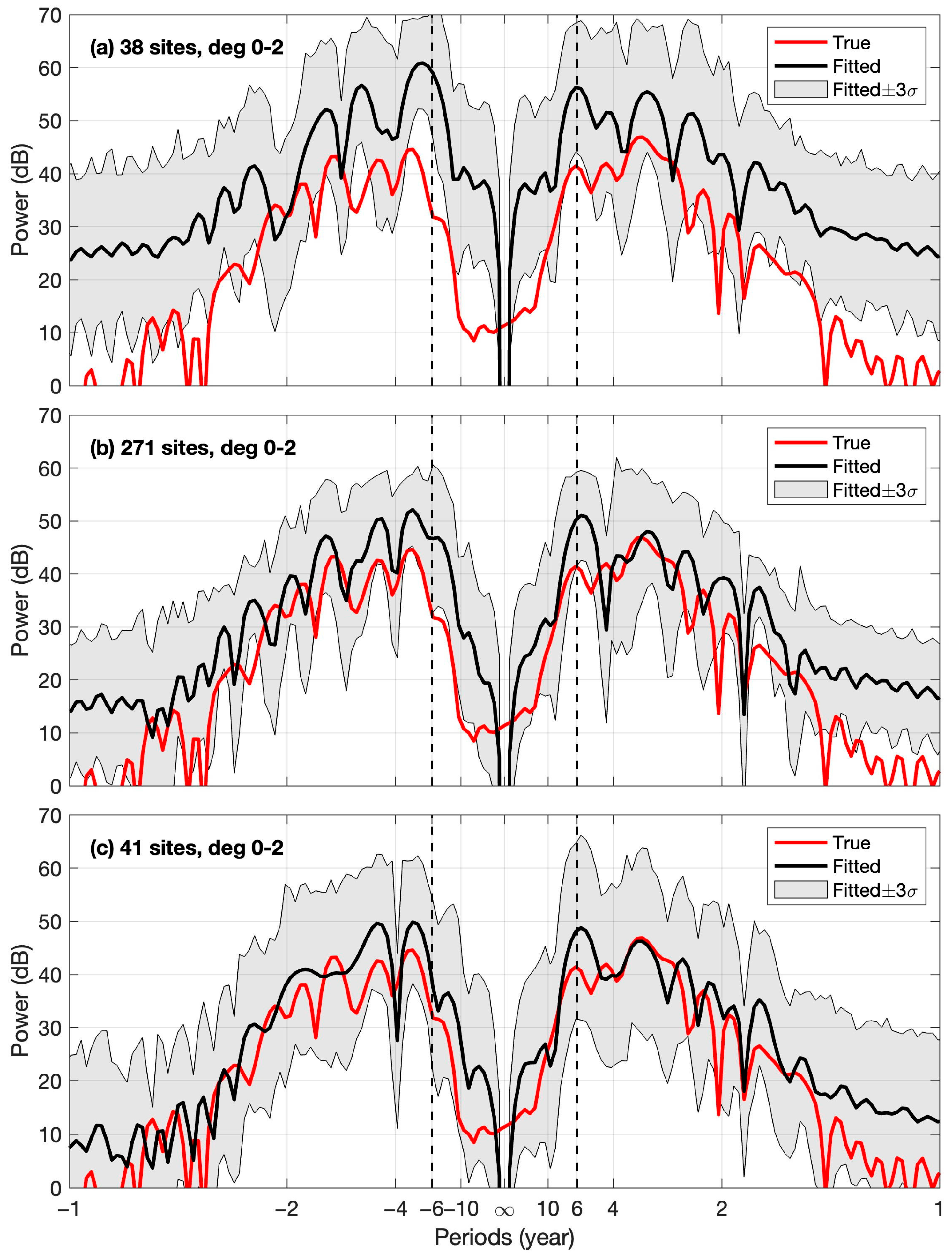
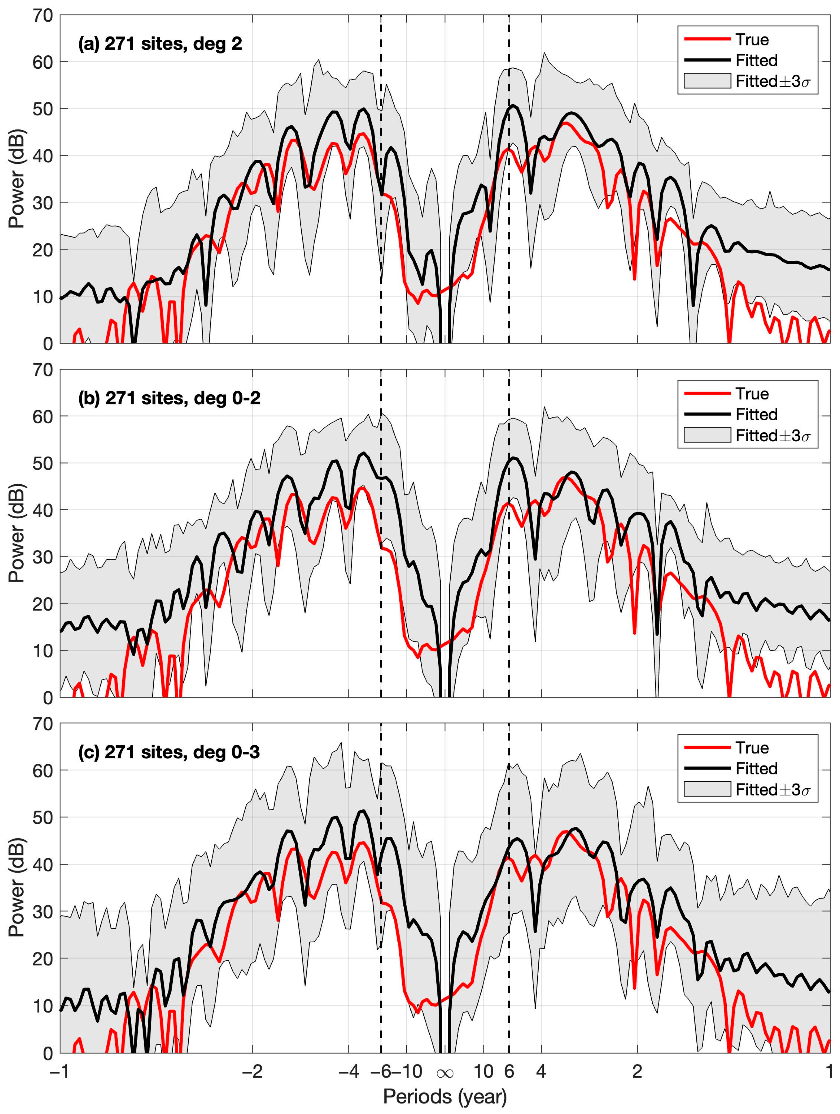
3.1. Synthetic Tests of SH Coefficient Estimation

To evaluate how LSQ estimates of [2, 2] coefficients varied with the number and spatial distribution of GPS stations, as well as with the number of SH coefficients being fit, we conducted a series of controlled experiments using synthetic data.

First, we generated synthetic time-varying global mass load fields representing climate-related signals from April 2002 to May 2023. These fields combined atmospheric, oceanic, and terrestrial hydrology loads and were constructed by summing GRACE/GRACE-FO dealiasing fields (AOD1B GAC) with GLDAS model outputs. The synthetic fields were expressed as SH expansions up to degree and order 100.

Second, these global fields were converted to vertical loading displacements at selected GPS station locations. To simulate observational uncertainty, randomly generated flicker noise with a variance of $3{\mathrm{m}\mathrm{m}}^2$—consistent with typical GPS time series residuals after removing linear trends and seasonal signals—was added to the displacements. Ensembles of 100 noise realizations were created for each test.

Third, LSQ fits were applied to the GPS station data to estimate SH coefficients. The station samples were weighted by ${\cos }^4\left(\mathrm{l}\mathrm{a}\mathrm{t}\mathrm{i}\mathrm{t}\mathrm{u}\mathrm{d}\mathrm{e}\right)$, because [2, 2] variations are largest at the equator, with variance proportional to the fourth power of the cosine of latitude. We tested cases of fitting coefficients to degree 2 only, degrees 0 through 2, and degrees 0 through 3 for both the 38 and 271 station sets and a subset of 41 with a more uniform distribution (as shown in Figure 1). The resulting LSQ estimates of the [2, 2] coefficients were then compared to their known true values from the synthetic fields.

Figure 4a–c show DFT periodogram spectra of ${\mathrm{C}}_{22}+i{\mathrm{S}}_{22}$ for the true (red curves) and ensemble means of estimates (black curves) using 38, 271, and 41 stations. In Figure 4 all coefficients from degrees 0 to 2 are fit. The LSQ annual, semi-annual components, and linear trends have been removed, and a two- to eight-year zero phase band-pass Butterworth filter was applied prior to spectral analysis. The gray-shaded areas indicate the 3σ confidence intervals (~99.7% confidence level) derived from an ensemble of 100. These results show that using 271 stations has an advantage in suppressing random observation noise, thus reducing areas of the 3σ confidence regions. The discrepancy between black and red curves in Figure 4a indicates that there was an overestimation of power by 10 to 20 dB with only 38 stations. Overestimations were reduced using both 271 and 41 stations, suggesting this effect may have been related to the uneven geographical distribution of the 38 stations.

Figure 5 shows DFT periodogram spectra of ${\mathrm{C}}_{22}+i{\mathrm{S}}_{22}$ for the true (red curve) and ensemble means of the estimates (black curves) using 271 stations. Figure 5a–c illustrate the results when all coefficients were fit to degree 2 only, degrees 0 through 2, and degrees 0 through 3. A two- to eight-year zero-phase band-pass Butterworth filter was applied prior to spectral analysis. The gray area contains the 3σ confidence region of the ensemble of 100. These results show that fitting coefficients from the 0 through 3 degrees results was less effective in suppressing random noise, as evidenced by the larger 3σ confidence regions. The results for fitting coefficients from degree 2 only or degrees 0 through 2 were quite similar, and we adopted LSQ fits to degrees 0 through 2 in subsequent analyses.

The real-valued Morlet wavelet spectra of [2, 2] coefficients from the two experiments are presented in the Supplementary Information (Texts S1 and S2).

3.2. SYO Signals in GPS Observations

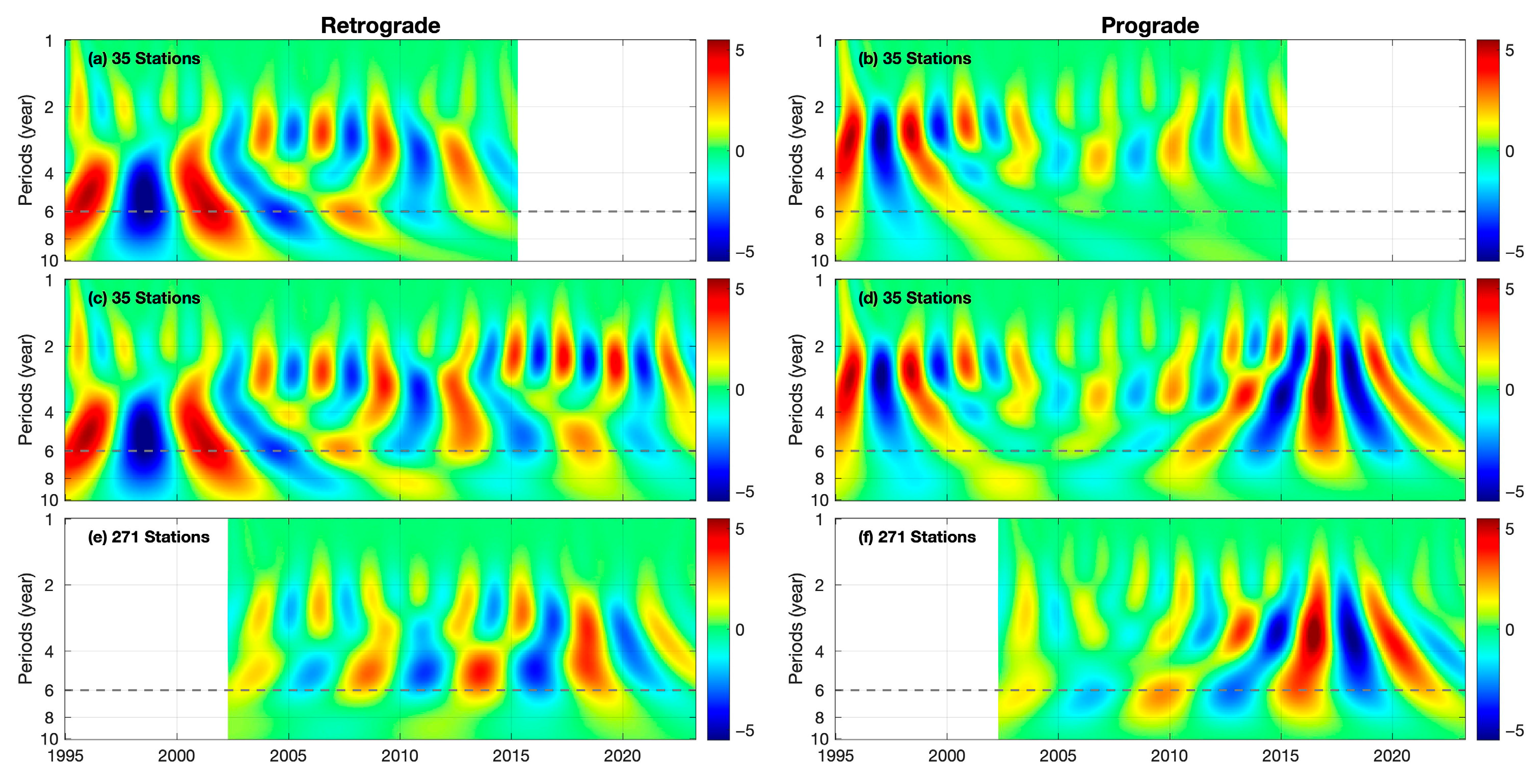
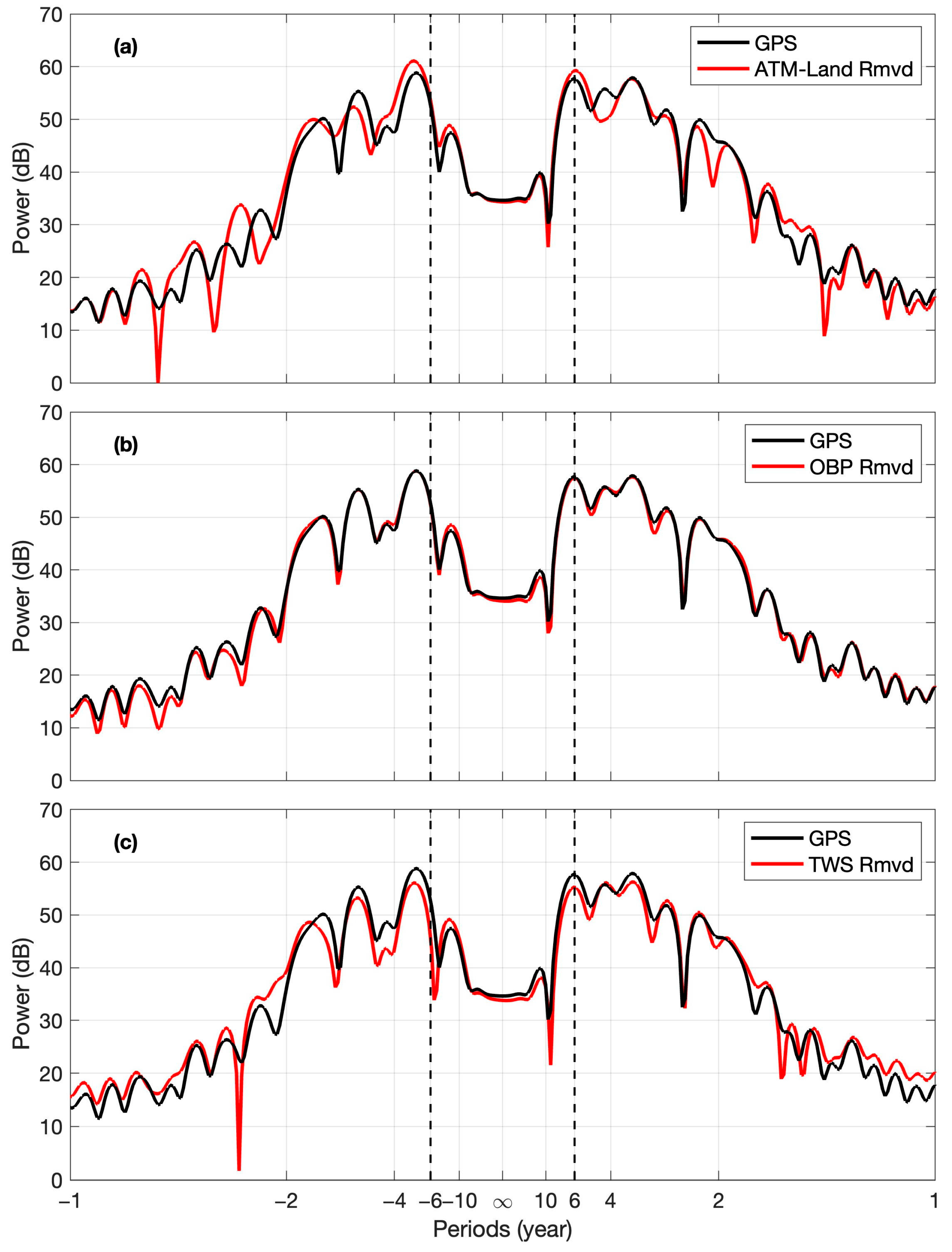
3.2.1. Spectral Analysis

To replicate the findings in [8], we first examined the same 38 GPS stations and time span (January 1995 to April 2015) and then extended the analysis through 2023. Three of the 38 stations (BRIB, BRMU, PIN2) did not have publicly available data for the extended period, possibly due to discontinued operation or other technical issues, and were excluded in our analysis. We also used the 271 stations shown in Figure 1 for the same analysis.

Figure 6 and Figure 7 compare DFT and wavelet spectra of ${\mathrm{C}}_{22}+i{\mathrm{S}}_{22}$, respectively. The case of 35 stations was computed for the two periods (January 1995 to April 2015 and January 1995 to April 2023). The longer time span (1995–2023) provided better frequency resolution (red curve in Figure 6). For both time spans in the 35-station case, a retrograde SYO spectral peak was evident and was larger than at the prograde frequency, consistent with the results presented in [8]. However, for the longer time span, the peak prograde SYO power (approximately at a 5.42-year period) increased by ~4 dB (black versus red curves in Figure 6), making the retrograde dominance less evident. The DFT periodogram using 271 stations (blue curve in Figure 6) shows that the retrograde dominance was even less evident and nearly disappeared. The wavelet spectra in Figure 7 show that prior to 2005, the retrograde SYO was strong but weakened after 2010. For the extended period, a prograde SYO became prominent after about 2010.

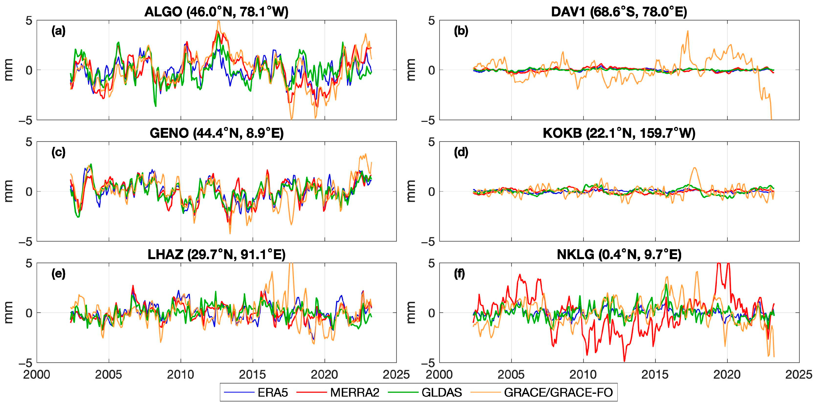
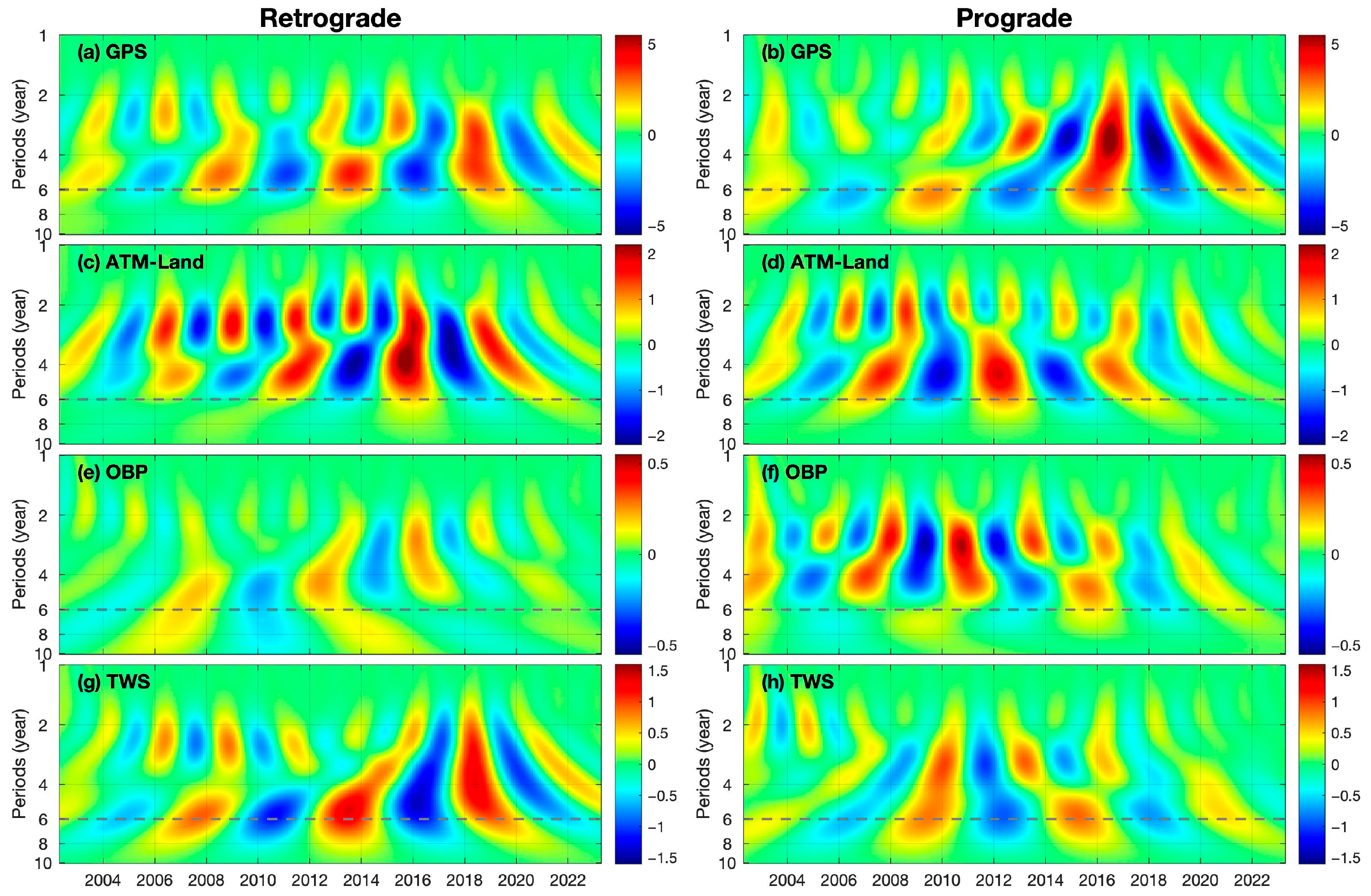
3.2.2. Surface Loading Effects

We first examined surface loading displacements from the atmosphere over the continents, OBP, and TWS using ERA5, ECCO2, ERA5 estimates, as noted earlier. Wavelet spectra and DFT periodograms for [2, 2] GPS series and loading estimates for the 271-station set are shown in Figure 8 and Figure S5 (for brevity), respectively. A prograde and retrograde SYO was evident in atmospheric and TWS loadings, whereas OBP loading showed less evidence of a SYO with varying amplitudes. TWS loading tended to be in phase with GPS [2, 2] displacements for both prograde and retrograde SYO, whereas atmospheric loading appeared out of phase with GPS displacements. The six-year phase $\phi$ was defined by $A\cos (\omega \left(t-t_0\right)-\phi )$, where $A$ is the amplitude, $t_0$ is the start of the year, and $\omega$ is ${\displaystyle \frac{1}{6}}$ cycles/year.

Table 1. Phase (in degrees) of the six-year periodic component for prograde and retrograde [2, 2] in GPS observations and environmental loadings.

	Retrograde	Prograde
GPS	341	218
ATM-Land	146	11
OBP	328	186
TWS	318	205

summarizes the phases from GPS and environmental loading estimates, further supporting the observed in-phase and out-of-phase relationships.

Figure 9 shows DFT periodogram spectra of GPS deformation after being corrected for individual climate-related loads. The corresponding wavelet spectra appear in Figure S6. For the chosen models in these initial experiments, the largest reduction in SYO power resulted from the correction with ERA5 TWS loading (Figure 9c) by about 1.4 dB at the retrograde peak near ~5.0-year and 1.2 dB at the prograde peak near ~6.1-year. Larger reductions were obtained using other TWS estimates, as discussed below. Correcting for atmospheric loading produced a slight increase in power, with the effect of OBP correction being quite small.

The contributions due to loading sources could be quantified by comparing the sinusoidal fits at periods near six years (corresponding to periodogram peaks) to [2, 2] GPS and loading displacements. The results for the six example stations are shown in Figure S7. TWS loading sinusoids tended to be in phase with the 271-station [2, 2] sinusoids, with amplitudes of ~24% of prograde and ~32% of retrograde GPS sinusoids. The amplitude of the atmospheric load over the continents was comparable to that of TWS, but the periods associated with periodogram peaks differed from those in GPS periodogram spectra. The result was that the sinusoids went in and out of phase. The OBP load was small, and the near-six-year spectral peaks of atmospheric loading over the continents appeared at 4.49-years prograde and 6.83-years retrograde. Note that SYO [2, 2] sinusoids represented quite small contributors to the displacement time series at individual stations. For example, at ALGO, the sinusoid amplitude associated with the spectral peak was only about 0.3 mm, contributing only ~10% to the standard deviation of the broad-band series, about 3 mm (black curves in Figure 2).

4. Discussion

The analysis above used ERA5 (for atmosphere and TWS) and ECCO2 (for ocean) loading calculations. We examined periodogram spectra of [2, 2] loading using the other models for the atmosphere (ERA5 and MERRA-2) and for TWS (ERA5, MERRA-2, GLDAS and GRACE/GRACE-FO).

DFT periodograms of band-pass filtered ${\mathrm{C}}_{22}+i{\mathrm{S}}_{22}$ from 271-station GPS vertical displacements and TWS load series are shown in Figure 10. All the TWS loading sources showed spectral peaks near positive and negative six-year periods, but there were distinct power differences. The GRACE/GRACE-FO TWS [2, 2] spectrum had the largest SYO power, especially for the retrograde component. ERA5 TWS, used in the earlier calculation, was the smallest. We could quantify the effect of TWS loading from the different estimates by computing the power difference ($∆\mathrm{d}\mathrm{B}$) at peak frequencies near ±six years of GPS and of TWS (black and colored curves in Figure 10). The $∆\mathrm{d}\mathrm{B}$ was converted to amplitude percentage via ${10}^{{\displaystyle \frac{∆\mathrm{d}\mathrm{B}}{20}}}\times 100\%$ in

Table 2. TWS loading contributions to GPS vertical displacement amplitudes of SH [2, 2] SYO from different models/observations.

	ERA5	MERRA-2	GLDAS	GRACE/GRACE-FO
Prograde	24%	51%	57%	56%
Retrograde	32%	49%	67%	93%

. The wide range of amplitudes in Table 2 shows that the TWS contribution to [2, 2] GPS deformation was highly uncertain. Thus, TWS may explain anywhere from a fraction to most of the observed SYO [2, 2] GPS variation. It is also interesting that the GRACE/GRACE-FO estimate, which represented a direct observation rather than a model, showed the largest amplitude. This was partly because satellite gravimetry captures a more comprehensive range of TWS components (e.g., groundwater depletion) than climate models, but it may also reflect potential overestimation in the GRACE/GRACE-FO estimate due to the inclusion of mass changes within the Earth’s interior.

Besides the periodograms of GPS and TWS load series shown in Figure 10, a comparison with TWS load-corrected series is also shown in Figure S8. There was reduced spectral power after applying TWS load corrections using any of the four models, further supporting the importance of TWS in the SYO GPS signals.

Due to the large differences among different TWS estimates, we applied the Three-Cornered Hat (TCH) method [35,36] to assess the uncertainties of [2, 2] based on these estimates. For a common signal (e.g., TWS-derived [2, 2]), each estimate can be represented as the sum of the true signal and a noise term, i.e., ${Estimate}_i=True+{Noise}_i$. By computing the variance of the difference between any two TWS estimates, thereby eliminating the common true signal, we obtained six equations involving four unknown noise variances, as shown in Equation (5). These unknowns can be solved using a LSQ approach; the results are presented in

Table 3. Standard deviation of the noise in [2, 2] from each TWS estimate.

	ERA5	MERRA-2	GLDAS	GRACE/GRACE-FO
${\mathrm{C}}_{22}$	$2.63\times {10}^{-11}$	$8.47\times {10}^{-12}$	$1.36\times {10}^{-11}$	$4.03\times {10}^{-11}$
${\mathrm{S}}_{22}$	$1.65\times {10}^{-11}$	$3.37\times {10}^{-11}$	$2.43\times {10}^{-12}$	$7.54\times {10}^{-11}$

.

$$\mathrm{v}\mathrm{a}\mathrm{r}\left({Noise}_i\right)+\mathrm{v}\mathrm{a}\mathrm{r}\left({Noise}_j\right)=\mathrm{v}\mathrm{a}\mathrm{r}\left({Estimate}_i-{Estimate}_j\right).$$

(5)

It is important to note that the uncertainties estimated from the TCH method should be interpreted in the context of the method’s assumptions and limitations. First, the underlying assumption of independence among the TWS estimates was not strictly met, as the model-based estimates (e.g., ERA5, MERRA-2, GLDAS) may have shared similar forcing data, parameterizations, or structural components. Second, the GRACE/GRACE-FO estimates contained observed signals—such as mass changes from groundwater, ice, and surface water—that were not fully represented in the land surface models. As a result, GRACE/GRACE-FO exhibited higher apparent noise variance in the TCH framework, which did not necessarily reflect lower data quality but rather a mismatch in signal content. Therefore, the uncertainties estimated by the TCH method should be regarded as approximate indicators rather than absolute measures and were best used for qualitative comparison or as a reference for uncertainty characterization.

Figure S9 shows that both a prograde and retrograde SYO persisted after atmospheric load correction using either model. There was an amplification of ~1 dB using the ERA5 model to correct for atmospheric loading, but the differences between the two models were minor. Our results are consistent with previous studies of SYO in ΔLOD [4,12,20,37], which reported that atmospheric angular momentum corrections enhance the SYO observed in ΔLOD. Different ocean models are reported to exhibit poor agreement at low SH degrees [23], highlighting uncertainties in representing large-scale ocean mass variability. Although the ECCO model suggested only a minor ocean contribution to SYO variations, this did not preclude the presence of unmodeled signals arising from limitations or simplifications in current ocean models. Imperfections, such as inadequate representation of deep ocean dynamics, boundary conditions, or data assimilation techniques, may have led to residual oceanic signals that were not fully captured, potentially contributing to the uncertainties in the SYO signal. Unmodeled non-linear variations in the current linear GIA model may also have contributed to the SYO signal.

The above analysis was conducted with monthly data samples, but we also examined daily station data and the wavelet spectra of [2, 2] coefficients. There were minor differences using daily data, and notably, Figure S10a bears a strong resemblance to Figure 3b in [8], confirming the same retrograde SYO signal found in their study using daily data. Similar to Figure 7, the daily data also showed a decrease in the strength of the retrograde SYO signal after 2010.

5. Conclusions

GPS vertical displacements showed SYO behavior, as reported in the literature [8,9]. Both the spatial distribution of GPS stations and details of the LSQ fitting affected the estimated variation. The uneven spatial distribution of GPS stations may have led to biases in estimating SYO power. We found an overestimation of SYO power in our 38-station synthetic data experiment, which was reduced when the station set was larger or more evenly distributed geographically. Synthetic data experiments also showed that with the spatial and temporal range of available GPS data, the SYO [2, 2] estimates may have been contaminated by observational noise and would have deteriorated if higher degree coefficients had been included in the LSQ fit.

We confirm the results presented in [8] using the same 35 stations, finding a dominant retrograde SYO using data from January 1995 to April 2015, but in the extended period to April 2023, the retrograde signal weakened while the prograde signal intensified, particularly after 2010. Additionally, retrograde dominance became much less significant in estimates using the more reliable 271-station set.

Morlet wavelet spectra of corrections appeared in-phase with the [2, 2] GPS vertical displacement signal, consistent with evidence of a SYO reported in GRACE/GRACE-FO data by [12]. Contributions from TWS load amplitudes varied considerably among different models/observations, ranging over values of 24%, 51%, 57%, and 56% of GPS prograde [2, 2] and 32%, 49%, 67%, and 93% of retrograde amplitudes using ERA5, MERRA-2, GLDAS, and GRACE/GRACE-FO, respectively. As noted above, the low spatial resolution of TWS fields and spatial sensitivity of the loading Green’s function might have led to an underestimate of TWS loading at individual stations. Our results indicate that the [2, 2] SYO signal may have been largely related to the surface loading effect. The rapid decline in retrograde dominance over the extended period of observation was also consistent with a near surface climatic source.

GPS continues to provide accurate observation of surface deformations, which is important for observing and investigating the global SYO deformation mode. Continuing to extend the record of GPS observations will provide essential insights into possible SYO sources within the Earth system and further enhance understanding of global dynamic and coupling processes.

References

1. Abarca Del Rio, R.; Gambis, D.; Salstein, D.A. Interannual Signals in Length of Day and Atmospheric Angular Momentum. Ann. Geophys. 2000, 18, 347–364. [Google Scholar] [CrossRef]
2. Djurović, D.; Pâquet, P. The Common Oscillations of Solar Activity, the Geomagnetic Field, and the Earth’s Rotation. Sol. Phys. 1996, 167, 427–439. [Google Scholar] [CrossRef]
3. Vondrák, J. The Rotation of the Earth between 1955.5 and 1976.5. Stud. Geophys. Geod. 1977, 21, 107–117. [Google Scholar] [CrossRef]
4. Chen, J.; Wilson, C.R.; Kuang, W.; Chao, B.F. Interannual Oscillations in Earth Rotation. JGR Solid Earth 2019, 124, 13404–13414. [Google Scholar] [CrossRef]
5. Silva, L.; Jackson, L.; Mound, J. Assessing the Importance and Expression of the 6 Year Geomagnetic Oscillation. J. Geophys. Res. 2012, 117, B10101. [Google Scholar] [CrossRef]
6. Chao, B.F.; Yu, Y. Variation of the Equatorial Moments of Inertia Associated with a 6-Year Westward Rotary Motion in the Earth. Earth Planet. Sci. Lett. 2020, 542, 116316. [Google Scholar] [CrossRef]
7. Dumberry, M. Gravity Variations Induced by Core Flows. Geophys. J. Int. 2010, 180, 635–650. [Google Scholar] [CrossRef]
8. Ding, H.; Chao, B.F. A 6-Year Westward Rotary Motion in the Earth: Detection and Possible MICG Coupling Mechanism. Earth Planet. Sci. Lett. 2018, 495, 50–55. [Google Scholar] [CrossRef]
9. Watkins, A.; Fu, Y.; Gross, R. Earth’s Subdecadal Angular Momentum Balance from Deformation and Rotation Data. Sci. Rep. 2018, 8, 13761. [Google Scholar] [CrossRef]
10. Meyer, P.G.; Kantz, H. A Simple Decomposition of European Temperature Variability Capturing the Variance from Days to a Decade. Clim. Dyn. 2019, 53, 6909–6917. [Google Scholar] [CrossRef]
11. Moreira, L.; Cazenave, A.; Palanisamy, H. Influence of Interannual Variability in Estimating the Rate and Acceleration of Present-Day Global Mean Sea Level. Glob. Planet. Change 2021, 199, 103450. [Google Scholar] [CrossRef]
12. Pfeffer, J.; Cazenave, A.; Rosat, S.; Moreira, L.; Mandea, M.; Dehant, V.; Coupry, B. A 6-Year Cycle in the Earth System. Glob. Planet. Change 2023, 229, 104245. [Google Scholar] [CrossRef]
13. Cazenave, A.; Pfeffer, J.; Mandea, M.; Dehant, V.; Gillet, N. Why is the Earth System Oscillating at a 6-Year Period? Surv. Geophys. 2025, 1–26. [Google Scholar] [CrossRef]
14. Chao, B.F. Dynamics of Axial Torsional Libration under the Mantle-inner Core Gravitational Interaction. JGR Solid Earth 2017, 122, 560–571. [Google Scholar] [CrossRef]
15. Gillet, N.; Jault, D.; Canet, E.; Fournier, A. Fast Torsional Waves and Strong Magnetic Field within the Earth’s Core. Nature 2010, 465, 74–77. [Google Scholar] [CrossRef]
16. Gross, R.S. Earth Rotation Variations—Long Period. In Treatise on Geophysics; Elsevier: Amsterdam, The Netherlands, 2007; Volume 3, ISBN 978-0-444-52748-6. [Google Scholar]
17. Mound, J.E.; Buffett, B.A. Interannual Oscillations in Length of Day: Implications for the Structure of the Mantle and Core. J. Geophys. Res. 2003, 108. [Google Scholar] [CrossRef]
18. Gillet, N.; Dumberry, M.; Rosat, S. The Limited Contribution from Outer Core Dynamics to Global Deformations at the Earth’s Surface. Geophys. J. Int. 2020, 224, 216–229. [Google Scholar] [CrossRef]
19. Pan, Y.; Jiang, W.; Ding, H.; Shum, C.K.; Jiao, J.; Xiao, Y.; Wu, Q. Interannual Variability of Vertical Land Motion over High Mountain Central Asia from GPS and GRACE/GRACE-FO Observations. GPS Solut. 2023, 27, 168. [Google Scholar] [CrossRef]
20. Cazenave, A.; Pfeffer, J.; Mandea, M.; Dehant, V. ESD Ideas: A 6-Year Oscillation in the Whole Earth System? Earth Syst. Dynam. 2023, 14, 733–735. [Google Scholar] [CrossRef]
21. Rosat, S.; Gillet, N.; Boy, J.-P.; Couhert, A.; Dumberry, M. Interannual Variations of Degree 2 from Geodetic Observations and Surface Processes. Geophys. J. Int. 2021, 225, 200–221. [Google Scholar] [CrossRef]
22. Dumberry, M.; Mandea, M. Gravity Variations and Ground Deformations Resulting from Core Dynamics. Surv. Geophys. 2022, 43, 5–39. [Google Scholar] [CrossRef] [PubMed]
23. Lecomte, H.; Rosat, S.; Mandea, M.; Boy, J.; Pfeffer, J. Uncertainty of Low-Degree Space Gravimetry Observations: Surface Processes Versus Earth’s Core Signal. JGR Solid Earth 2023, 128, e2023JB026503. [Google Scholar] [CrossRef]
24. Argus, D.F.; Landerer, F.W.; Wiese, D.N.; Martens, H.R.; Fu, Y.; Famiglietti, J.S.; Thomas, B.F.; Farr, T.G.; Moore, A.W.; Watkins, M.M. Sustained Water Loss in California’s Mountain Ranges During Severe Drought from 2012 to 2015 Inferred from GPS. J. Geophys. Res. Solid Earth 2017, 122, 10559–10585. [Google Scholar] [CrossRef]
25. Heflin, M.; Donnellan, A.; Parker, J.; Lyzenga, G.; Moore, A.; Ludwig, L.G.; Rundle, J.; Wang, J.; Pierce, M. Automated Estimation and Tools to Extract Positions, Velocities, Breaks, and Seasonal Terms from Daily GNSS Measurements: Illuminating Nonlinear Salton Trough Deformation. Earth Space Sci. 2020, 7, e2019EA000644. [Google Scholar] [CrossRef]
26. Gegout, P.; Boy, J.-P.; Hinderer, J.; Ferhat, G. Modeling and Observation of Loading Contribution to Time-Variable GPS Sites Positions. In Gravity, Geoid and Earth Observation: IAG Commission 2: Gravity Field, Chania, Crete, Greece, 23–27 June 2008; Mertikas, S.P., Ed.; Springer: Berlin/Heidelberg, Germany, 2010; Volume 135, pp. 651–659. [Google Scholar]
27. Mémin, A.; Boy, J.-P.; Santamaría-Gómez, A. Correcting GPS Measurements for Non-Tidal Loading. GPS Solut. 2020, 24, 45. [Google Scholar] [CrossRef]
28. Save, H. CSR GRACE and GRACE-FO RL06 Mascon Solutions V02; The University of Texas at Austin: Austin, TX, USA, 2020. [Google Scholar] [CrossRef]
29. Save, H.; Bettadpur, S.; Tapley, B.D. High-Resolution CSR GRACE RL05 Mascons. J. Geophys. Res. Solid Earth 2016, 121, 7547–7569. [Google Scholar] [CrossRef]
30. Farrell, W.E. Deformation of the Earth by Surface Loads. Rev. Geophys. Space Phys. 1972, 10, 761–797. [Google Scholar] [CrossRef]
31. Han, D.; Wahr, J. The Viscoelastic Relaxation of a Realistically Stratified Earth, and a Further Analysis of Postglacial Rebound. Geophys. J. Int. 1995, 120, 287–311. [Google Scholar] [CrossRef]
32. Chao, B.F.; Naito, I. Wavelet Analysis Provides a New Tool for Studying Earth’s Rotation. EoS Trans. 1995, 76, 161–165. [Google Scholar] [CrossRef]
33. Morlet, J.; Arens, G.; Fourgeau, E.; Giard, D. Wave Propagation and Sampling Theory—Part II: Sampling Theory and Complex Waves. Geophysics 1982, 47, 222–236. [Google Scholar] [CrossRef]
34. Pan, Y.; Chen, R.; Ding, H.; Xu, X.; Zheng, G.; Shen, W.; Xiao, Y.; Li, S. Common Mode Component and Its Potential Effect on GPS-Inferred Three-Dimensional Crustal Deformations in the Eastern Tibetan Plateau. Remote Sens. 2019, 11, 1975. [Google Scholar] [CrossRef]
35. Premoli, A.; Tavella, P. A Revisited Three-Cornered Hat Method for Estimating Frequency Standard Instability. IEEE Trans. Instrum. Meas. 1993, 42, 7–13. [Google Scholar] [CrossRef]
36. Wang, S.Y.; Li, J.; Chen, J.; Hu, X. Uncertainty Assessments of Load Deformation from Different GPS Time Series Products, GRACE Estimates and Model Predictions: A Case Study over Europe. Remote Sens. 2021, 13, 2765. [Google Scholar] [CrossRef]
37. Rekier, J.; Chao, B.F.; Chen, J.; Dehant, V.; Rosat, S.; Zhu, P. Earth’s Rotation: Observations and Relation to Deep Interior. Surv. Geophys. 2022, 43, 149–175. [Google Scholar] [CrossRef]
Figure 1. Locations of the 38 GPS stations used in [8] (green dots), and 271 (red dots) GPS stations; 41 blue triangle stations were a subset of the 271 chosen for a more uniform geographical distribution as described below. Example (gold star) stations (Figure 2) were ALGO (North America), DAV1 (Antarctica), GENO (Southern Europe), KOKB (Central Pacific), LHAZ (Central Asia), and NKLG (West Africa).
Remotesensing 17 01509 g001
Figure 2. GPS vertical displacements (black curves) and total environmental vertical loading displacements (atmospheric, OBP, and TWS from selected models as described below) (red curves) at the (a) ALGO, (b) DAV1, (c) GENO, (d) KOKB, (e) LHAZ, and (f) NKLG stations. Breaks and jumps, annual and semi-annual terms, and linear trends have been removed. The differences between GPS displacements and model predictions at KOKB and NKLG were mainly caused by the inaccuracy of the atmospheric model for a mid-ocean island (KOKB) and coastal area (NKLG).
Remotesensing 17 01509 g002
Figure 3. TWS load vertical displacements from ERA5, MERRA-2, GLDAS, and GRACE/GRACE-FO at the (a) ALGO, (b) DAV1, (c) GENO, (d) KOKB, (e) LHAZ, and (f) NKLG stations. Annual and semi-annual terms and linear trends have been removed.
Remotesensing 17 01509 g003
Figure 4. DFT periodograms of C 22 + i S 22 : true (red) and ensemble means of LSQ estimates (black) with randomly generated flicker noise at (a) 38 sites, (b) 271 sites, and (c) 41 sites. The gray area contains the 3σ confidence region. Station data are latitude weighted as described in the text, and all coefficients from degrees 0 to 2 were estimated simultaneously. A two- to eight-year band-pass filter was applied prior to spectral analysis.
Remotesensing 17 01509 g004
Figure 5. DFT periodograms of C 22 + i S 22 : true (red) and ensemble means of LSQ estimates (black) with randomly generated flicker noise at 271 sites. All coefficients from (a) degree 2 only, (b) degree 0 through 2, and (c) degree 0 through 3 were estimated simultaneously. The gray area contains the 3σ confidence region. Station data are latitude weighted as described in the text. A two- to eight-year band-pass filter was applied prior to spectral analysis.
Remotesensing 17 01509 g005
Figure 6. DFT periodogram of C 22 + i S 22 estimated from 35 and 271 GPS-station sets over different time spans.
Remotesensing 17 01509 g006
Figure 7. Morlet wavelet spectra of band-pass filtered C 22 + i S 22 estimated from 35 (ad) and 271 (e,f) GPS-station sets. Retrograde and prograde signals are shown in the left and right columns, respectively. (a,b) are from January 1995 to April 2015; (c,d) are from January 1995 to April 2023; (e,f) are from May 2002 to April 2023. Spectral magnitudes have been scaled by 1 × 10 11 .
Remotesensing 17 01509 g007
Figure 8. Morlet wavelet spectra of band-pass filtered C 22 + i S 22 estimated from 271 GPS vertical displacements and individual vertical loading displacements from different sources. Retrograde and prograde signals are in the left and right columns, respectively. (a,b) from observed GPS vertical displacements; (c,d) from atmospheric loading over the continent; (e,f) from OBP loading; (g,h) from TWS loading. Spectral magnitudes are scaled by 1 × 10 11 .
Remotesensing 17 01509 g008
Figure 9. DFT periodograms of C 22 + i S 22 estimated from 271 GPS stations (black curves) and GPS minus individual loading contributions from (a) atmosphere over the continents, (b) OBP (c) TWS (red curves).
Remotesensing 17 01509 g009
Figure 10. DFT periodogram of C 22 + i S 22 estimated from 271 GPS station heights (black curve) and TWS loading using ERA5 (red curve), MERRA-2 (blue curve), GLDAS (green curve), and GRACE/GRACE-FO (magenta curve) models/observations.
Remotesensing 17 01509 g010