Mapping Trails and Tracks in the Boreal Forest Using LiDAR and Convolutional Neural Networks

Abstract

Trails and tracks are the detectable signs of passage of wildlife and off-highway vehicles in natural landscapes. They record valuable information on the presence and movement of animals and humans. However, published works aimed at mapping trails and tracks with remote sensing are nearly absent from the peer-reviewed literature. Here, we demonstrate the capacity of high-density LiDAR (light detection and ranging) and convolutional neural networks to map undifferentiated trails and tracks automatically across a diverse study area in the Canadian boreal forest. We compared maps developed with LiDAR from a drone platform (10 cm digital terrain model) with those from a piloted-aircraft platform (50 cm digital terrain model). We found no significant difference in the accuracy of the two maps. In fact, the piloted-aircraft map (F1 score of 77 ± 9%) performed nominally better than the drone map (F1 score of 74 ± 6%) and demonstrated a better balance among error types. Our maps reveal a 2829 km network of trails and tracks across the 59 km² study area. These features are especially abundant in peatlands, where the density of detected trails and tracks was 68 km/km². We found a particular tendency for wildlife and off-highway vehicles to adopt linear industrial disturbances like seismic lines into their movement networks. While linear disturbances covered just 7% of our study area, they contained 27% of all detected trails and tracks. This type of funnelling effect alters the movement patterns of humans and wildlife across the landscape and impedes the recovery of disturbed areas. While our work is a case study, the methods developed have broader applicability, showcasing the potential to map trails and tracks across large areas using remote sensing and convolutional neural networks. This capability can benefit diverse research and management communities.

1. Introduction

In many environments, the presence and movement of animals and humans can be revealed by their tracks and trails. Trails and tracks are the detectable signs of passage left by individuals or groups as they traverse the landscape. They can be transient or semi-permanent, depending on the substrate and frequency of use. Generally, tracks mark the passage of a single individual, while trails denote repeated use. Their morphology depends on the substrate and frequency of use. Softer substrates and higher frequencies of use are expected to generate more distinct trails and tracks. Harder substrates and less-frequent passage would create less distinct features. Trails and tracks may be constructed purposefully to facilitate efficient movement (e.g., [1]) or left behind by coincidental passage (e.g., [2]).

Many ecological and wildlife conservation applications require information on organism presence and movement, including habitat selection studies (e.g., [3,4]), population density assessments (e.g., [5,6]), and animal movement models (e.g., [7,8]). Most contemporary researchers track wildlife through global navigation satellite systems (GNSSs; e.g., [9]), camera traps (e.g., [10]), or genetics (e.g., [11]). Each of these efforts could benefit from complementary information on trails and tracks.

Previous authors have pointed out the influence of trails on wildlife detection probabilities in camera trap studies. For example, Harmsen et al. [12] reported that neotropical mammals varied substantially in their use of existing trails. In the authors’ Belizean study area, pumas (Puma concolor) followed trails more closely than jaguars (Panthera onca) in the same habitat type. As a result, density models of such species that fail to account for detection bias in cameras set on wildlife trails can produce misleading results. With reliable trail maps, researchers could not only parameterize their wildlife density models more effectively but also design camera trap studies that take the existing trail network into account. This could help make efficient use of limited resources [13].

Maps of human trails and tracks could also enhance our understanding and mitigation of anthropogenic disturbances on ecosystems. For example, previous studies have demonstrated the negative effects of mechanical trails and tracks on soil characteristics [14,15], the distribution of invertebrates [16], runoff patterns [17], erosion [18], and vegetation growth [14,19,20]. Many of these effects are especially pronounced in boreal peatlands, where the disturbance of sensitive organic substrates can have far-reaching implications on soil physical and chemical properties [21], plant community composition [22], methane emissions [23], and patterns of vegetation recovery [24].

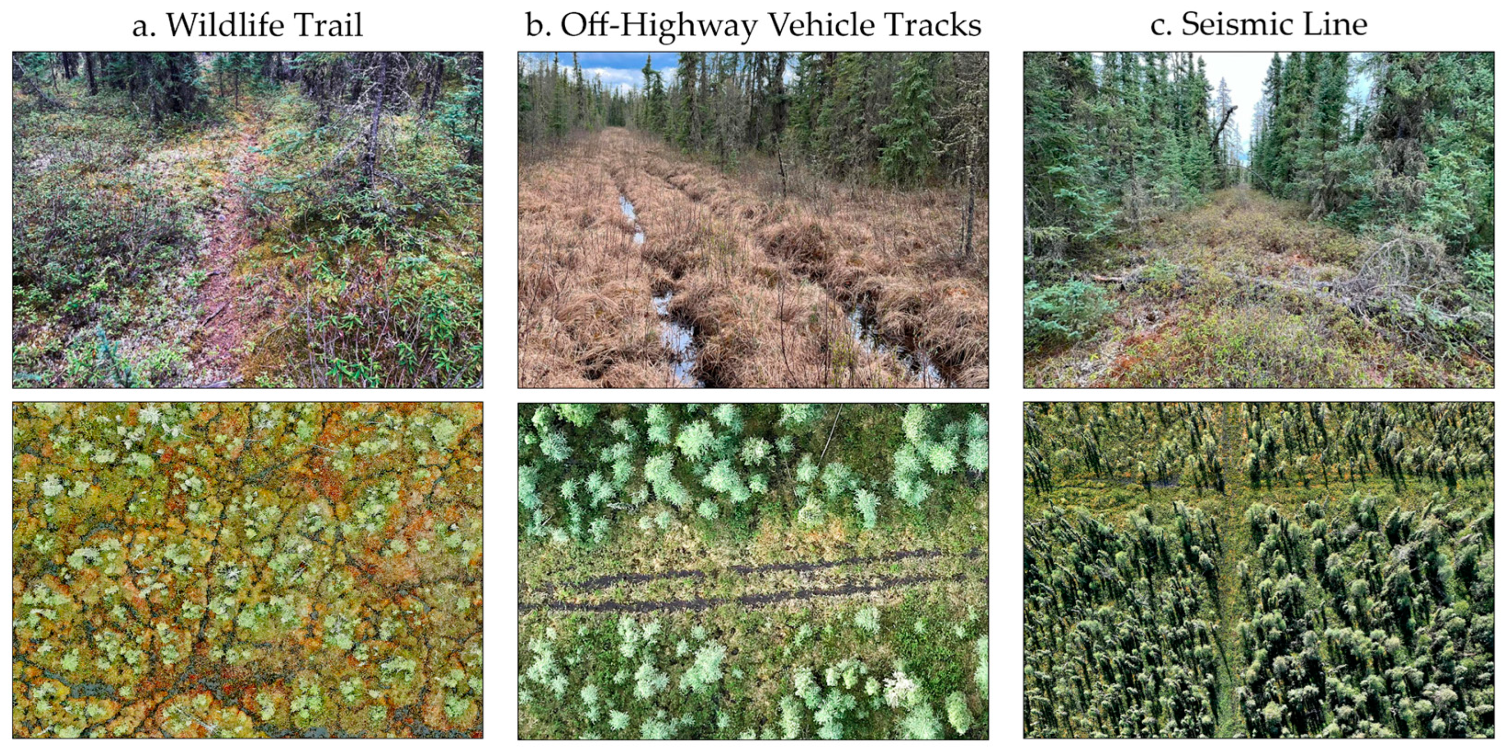
1.1. Mapping Trails and Tracks

Previous researchers have mapped trails and tracks directly through GNSS surveys (e.g., [25,26]) and volunteered geographic information (e.g., [27,28]), or indirectly through remote sensing. This study focuses on indirect remote-sensing approaches. On this subject, the literature is limited. The great majority of peer-reviewed research in this application domain has focused on mapping all-weather roads. Abdollahi et al. [29] provides a recent review of this subject. Studies in this application domain typically target wide, flat roads with distinct surface materials, making these methods less applicable to the detection of narrow, natural trails and tracks. Therefore, while some techniques might be adapted, trail and track mapping applications generally differ from road detection.

The body of peer-reviewed research focused on the automated detection of trails and tracks in natural areas using remote sensing is quite limited. Some studies have assessed the indirect effects of concentrated animal activity on vegetation using spectral indices (e.g., [30,31,32]), but these do not attempt to detect or map trails and tracks directly. Welch et al. [33] mapped 2950 km of off-highway vehicle trails in Everglades National Park, Florida, using 1:40,000 colour-infrared aerial photos. Kaiser et al. [34] mapped smuggler trail networks in the U.S.–Mexico border region of California using 60 cm four-band multispectral imagery. However, both studies relied extensively on heads-up digitizing. Kaiser et al. [34] also evaluated image enhancement and automated feature extraction routines. However, the authors’ best results relied on manual interpretation, feature delineation, and manual editing. Persistent noise, occlusions, and the variable nature of detectable mapping signals have largely prevented the use of automated workflows for mapping trails and tracks to this point.

Fully automated strategies for detecting and mapping trails and tracks using modern datasets and processing workflows are just now beginning to emerge, powered largely by recent advances in artificial intelligence. For example, Yamato et al. [35] used convolutional neural networks (CNNs) to map dugong (Dugong dugong) feeding trails from 0.47 cm resolution optical drone imagery in the intertidal seagrass beds of Trang Province, Thailand, with F1 scores of up to 0.895. Bhatnagar et al. [36] used a deep-learning image segmentation algorithm on drone-based orthomosaics to map wheel rut trails caused by mechanical harvesting machines in forest harvest blocks in Norway with an average F1 score of 0.77.

Recent studies have begun exploring automated trail and track detection with remote sensing, though applications remain limited in both scope and geography. The potential of CNNs and other forms of artificial intelligence to map trails and tracks over large terrestrial areas using high-resolution airborne datasets is largely untapped.

We are particularly interested in the capacity of high-density LiDAR (light detection and ranging) data to detect trails and tracks. While optical imagery also provides a promising information source, these data have limited canopy penetration abilities and are subject to frequent shadows in vegetated terrain. Other authors have recently begun using LiDAR to map drainage ditches (e.g., [37,38,39,40]). Whether these types of morphometric imprints could also be used to map trails and tracks more broadly remains untested in the context of trail and track detection.

1.2. Research Objectives

Our goal is to create tools and processing workflows for mapping trails and tracks automatically over large terrestrial areas using remote sensing. To achieve this goal, we established three research objectives, which are the subject of this paper:

• To demonstrate the capacity of high-density LiDAR and CNNs to map trails and tracks automatically in a natural environment;
• To compare the accuracy of trail/track maps developed with LiDAR from a drone platform (185 points/m²) and a piloted-aircraft platform (30 points/m²) to evaluate trade-offs between spatial resolution and operational scalability; and
• To measure the abundance and distribution of tracks and trails across different land-cover classes and their co-location with anthropogenic disturbances across our study area in the Canadian boreal forest.

To our knowledge, this is the first study on the use of LiDAR and CNNs for mapping terrestrial trails and tracks to appear in the peer-reviewed literature. Our research demonstrates that not only can trails and tracks be detected accurately with remote sensing under the correct conditions, but that high-quality maps can be obtained over large areas using data from piloted aircraft. While drone platforms deliver very high-resolution data, their operation can be limited by line-of-sight restrictions, battery life, and regulatory constraints. Piloted-aircraft platforms can be more practical for mapping large or inaccessible areas. Assessing their performance helps to establish scalable solutions. While our work is a case study, our findings reveal the potential for these workflows across a variety of exciting applications.

2. Materials and Methods

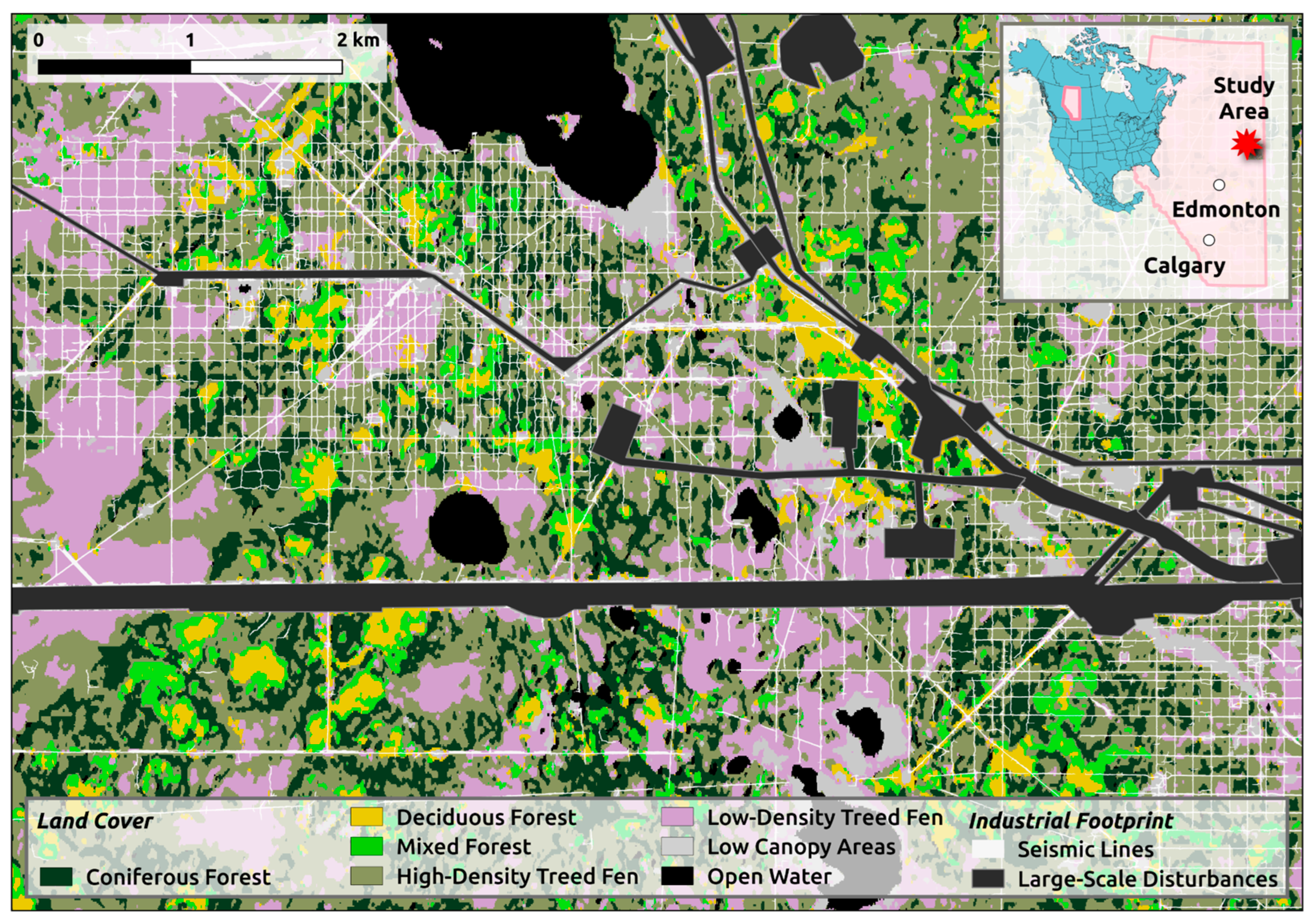
2.1. Study Area

Our study area is in the boreal forest of northeastern Alberta, Canada (Figure 1) at a site approximately 150 km south of Fort McMurray. The study area is in the central mixedwood natural subregion, located 500–600 m above sea level. The central mixedwood subregion has a continental subarctic climate characterized by cold winters and short, warm summers. Precipitation is moderate, with an average annual rainfall of around 400 to 600 mm [41].

Figure 1. Our 59 km² study site is in northeastern Alberta, Canada. It contains a diverse mosaic of land-cover types, from sparsely treed lowlands to thickly treed uplands.

Figure 1. Our 59 km² study site is in northeastern Alberta, Canada. It contains a diverse mosaic of land-cover types, from sparsely treed lowlands to thickly treed uplands.

Our 59 km² study area contains a diverse mosaic of land-cover types, from sparsely treed peatlands to thickly treed uplands (Figure 1). Peatlands—wetlands with accumulated organic materials [42]—cover 58% of the study area. Another 27% of the area is composed of uplands and transitional areas. This blend is typical of the central mixedwood parts of the boreal forest. Conifer trees dominate the peatland and transitional portions of the study area. Coniferous, deciduous, and mixedwood stands can be found on the upland portions. The remaining 15% of the area is covered by open water, roads, and large-scale industrial disturbances. We excluded these areas from most analyses.

There are three types of trails and tracks common to our study area: wildlife trails, off-highway vehicle (OHV) tracks, and seismic lines (Figure 2). Wildlife trails at our site are created primarily by the movements of ungulates like woodland caribou (Rangifer tarandus caribou) and white-tailed deer (Odocoileus virginianus). OHV tracks are wheel ruts created by off-road vehicles. Seismic lines are linear corridors left behind by mulchers and other heavy machinery used to cut clearings for subsurface petroleum exploration [43]. There are significant morphological differences between the three types. Wildlife trails (Figure 2a) are typically up to a metre wide and can form dense, intertwining networks. OHV tracks (Figure 2b) are like wildlife trails but normally appear as paired depressions created by OHV wheels. Seismic lines (Figure 2c) are 4 to 6 m wide mechanical cuts that have been installed in a systematic grid, with a spacing of about 100 m. The models we developed for this study are aimed at wildlife trails and OHV trails and tracks. We did not target seismic lines in this work.

Figure 2. Wildlife trails (a), off-highway vehicle tracks (b), and seismic lines (c) are the three types of trails and tracks common to our study area. Ground-level (top row) and aerial-view (bottom row) examples of all three features are shown.

Figure 2. Wildlife trails (a), off-highway vehicle tracks (b), and seismic lines (c) are the three types of trails and tracks common to our study area. Ground-level (top row) and aerial-view (bottom row) examples of all three features are shown.

While there are substantial morphological differences between wildlife trails, OHV trails and tracks, and seismic lines in our study area, they are not always physically separated from one another. In fact, OHVs and wildlife often adopt seismic lines into their transportation networks. Quantifying the amount of wildlife- and OHV-adopted seismic lines that exist in our study area was one of our research objectives.

2.2. Data Acquisition and Processing

Aerial LiDAR was provided by Alberta-Pacific Forest Industries, Inc., through partnership in the Boreal Ecosystem Recovery and Assessment (BERA) project (www.bera-project.org). The LiDAR was collected in the summer of 2022 with a Riegl VQ-1560ii system. The sensor was flown on a piloted aircraft at approximately 1800 m above ground level with a ± 60° maximum scan angle, an 825 kHz pulse repetition frequency, and a 50% swath side lap. The final point cloud had a density of 30 points/m². The vendor, Airborne Imaging, calibrated the dataset using precise point positioning (PPP) techniques to model and remove GNSS system errors. The horizontal and vertical accuracy were reported as 0.35 m and 0.20 m, respectively. Point-cloud classification was also performed by the vendor. We created 50 cm digital terrain models (DTMs) from classified ground points using the las2dem tool in LAStools version 2.0.1.

Drone data were collected for a subsection of our study area in the summer of 2022 using a Zenmuse L1 LiDAR sensor aboard a DJI Matrice 300 RTK. The sensor was flown approximately 100 m above ground level with triple-return mode and repetitive scanning enabled at a sampling rate of 160 kHz. The L1 sensor uses a near-infrared laser (905 nm), and the final point cloud had an average density of 185 points/m². The drone had RTK (real-time kinematic) positioning enabled and was connected to a DJI D-RTK 2 GNSS base station. We used PPP to obtain the final position of the base station, then calculated the difference between the final and initial base station positions. This difference was then applied to shift the point cloud into a corrected position.

To evaluate the drone LiDAR’s vertical accuracy, we conducted an RTK-GNSS survey using six independent checkpoint targets. These checkpoints were 1 × 1 m plastic targets that were laid out flat across the study area prior to drone flights. The targets coincided with 377 LiDAR points. The mean absolute error between the check point targets’ GNSS-surveyed elevation and the drone’s LiDAR-surveyed elevation was 3 cm.

We performed a variety of standard post-processing steps (e.g., noise removal and ground classification) on the drone-based point cloud using LAStools. We then generated a 10 cm DTM from the classified ground points using a k-nearest neighbour inverse-distance-weighted algorithm (knnidw; k = 10, p = 2) in the R package lidR [44,45].

The use of different DTM generation methods for the drone and piloted-aircraft data reflects differences in point density and preprocessing requirements between the two datasets. The vendor-supplied piloted-aircraft data were processed with las2dem due to their standardized classification and moderate density (30 pts/m²). The higher-density drone data (185 pts/m²) were interpolated using a k-nearest neighbour inverse distance weighting algorithm (knnIDW) in lidR to better preserve fine-scale topographic detail in complex terrain.

In the summer of 2023, we collected a sub-centimetre-resolution optical dataset over a subsection of our study area to provide reference data for independent testing. This subsection was a 0.25 km² portion of a low-density treed fen labelled Testing Area in Figure 3. These data were acquired using a DJI Zenmuse P1 sensor (full-frame 45-megapixel camera with a 35 mm lens) on the same drone platform that was used to collect the LiDAR. The drone was flown 35 m above ground level with RTK positioning enabled. The side and front overlap was set to 70% and 80%, respectively. This imagery was processed into an ultra-high-resolution (0.5 cm) true-colour orthomosaic using PIX4Dmapper. Like the drone LiDAR processing, the orthomosaic was shifted based on the difference between the initial and final base station positions, following PPP processing. A GNSS survey of 20 independent check points was used to assess the mean absolute error (0.11 m) and root mean square error (0.13 m) of the orthomosaic position.

Figure 3. Working within the training portion of the study area (large blue square), we extracted training patches cropped around 6395 random points (white dots in (a)). These 512 × 512-pixel training patches (b) were labelled using a preliminary U-Net model. These patches were then used to train a second, more refined set of U-Net models: one for the 10 cm drone data and a second for the 50 cm piloted-aircraft data. We tested the accuracy of these models in a physically independent test area (small red square) containing 11 randomly distributed testing polygons (red dots).

Figure 3. Working within the training portion of the study area (large blue square), we extracted training patches cropped around 6395 random points (white dots in (a)). These 512 × 512-pixel training patches (b) were labelled using a preliminary U-Net model. These patches were then used to train a second, more refined set of U-Net models: one for the 10 cm drone data and a second for the 50 cm piloted-aircraft data. We tested the accuracy of these models in a physically independent test area (small red square) containing 11 randomly distributed testing polygons (red dots).

We assume accurate coregistration between the three remote-sensing datasets used in this study: drone LiDAR, piloted-aircraft LiDAR, and drone orthomosaic. All three were captured following rigorous survey practices and produced very high-spatial-accuracy statistics. We further assume that there are no substantial differences in the pattern of trails and tracks within our remote study area between the summer of 2022, when the LiDAR data were collected, and the summer of 2023, when the optical data were collected. The LiDAR data were used to build the trail/track models, while the optical data were used for accuracy assessment. We contend that any differences, should they exist, would not serve to bias one LiDAR dataset over the other and would therefore have no material effect on our experiments.

2.3. Mapping Trails and Tracks

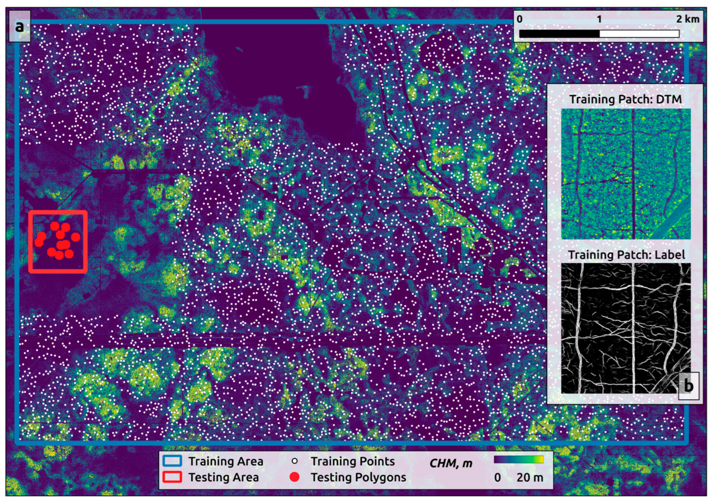
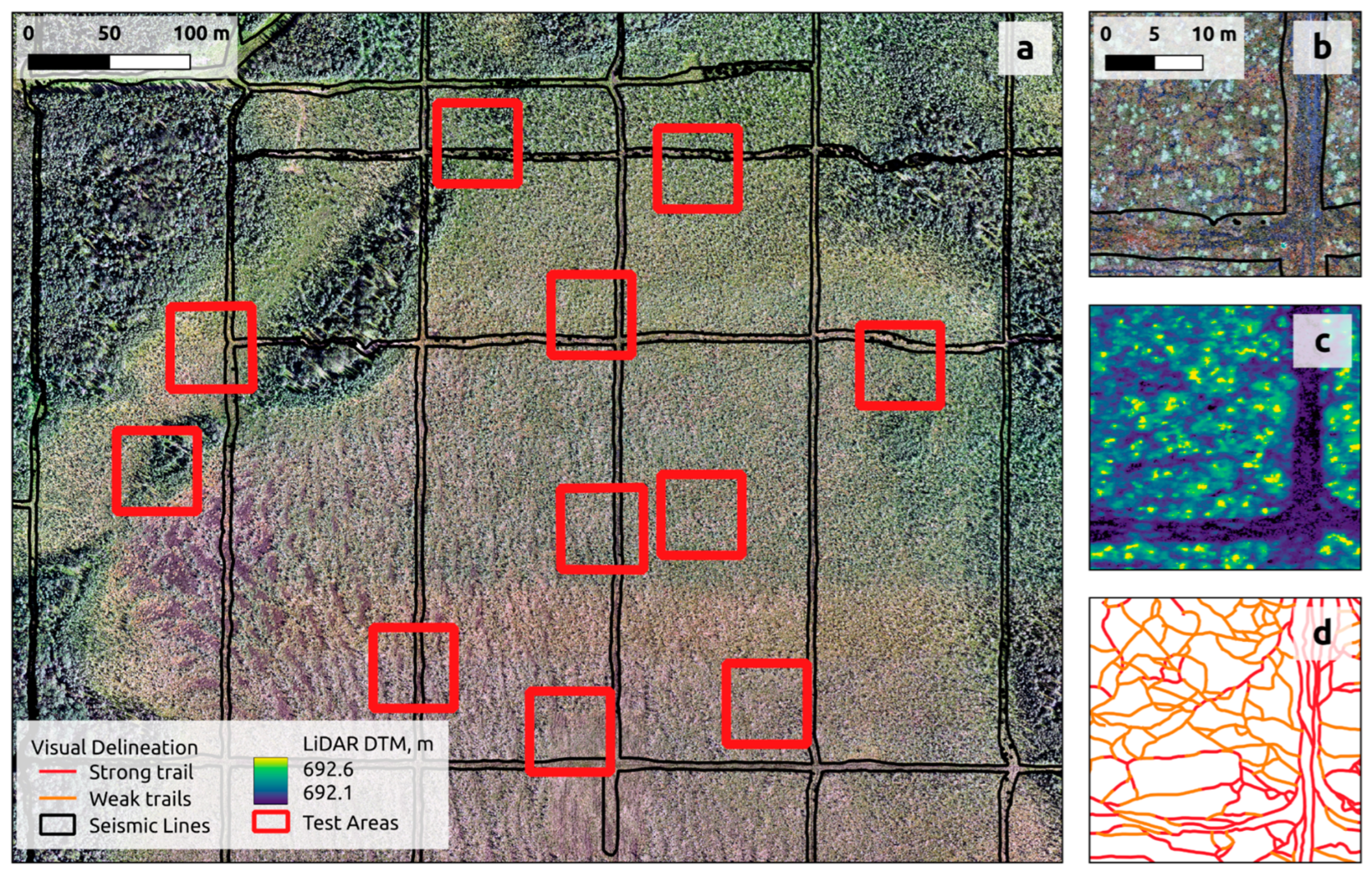
2.3.1. Training Data Preparation

We adopted a progressive refinement approach to training data preparation and labelling. First, we used visual interpretation of aerial LiDAR data to manually label a preliminary training dataset. Labels were created by visually interpreting rasterized 50 cm DTMs derived from the piloted-aircraft LiDAR data. Trail and track features were delineated manually by expert interpreters using QGIS 3.34.10-Prizren, based on their morphometric appearance in the terrain models. No point-cloud labelling was performed. An initial U-Net model was trained using the manually labelled patches. This model’s predictions were used to generate a refined set of labels for final model training on both the 10 cm and 50 cm DTMs. To ensure quality, we manually inspected the output from the initial model and corrected errors prior to using them as labels in the second-stage training. This hybrid approach allowed us to accelerate label creation while maintaining control over training data quality

The main training set consisted of 6395 training patches cropped around random points distributed across the training portion of our study area, which covered 45 km² (Figure 3a). Each patch was 512 × 512 pixels in size and contained both DTM data and pixel-wise binary labels (Figure 3b). Each DTM patch was independently normalized to a 0–1 range using min–max scaling. No further transformations were applied. To improve the segmentation quality at this second stage, we removed objects smaller than 30 pixels from the binary masks. Finally, we thinned the segmented features (trails and tracks) to a skeletal form, then buffered them back to standardized widths appropriate to each resolution—1 pixel (50 cm) for the 50 cm DTM, and 3 pixels (30 cm) for the 10 cm DTM—to represent approximate real-world trail widths. This process produced trails and tracks with standardized widths in the binary masks.

We used several augmentation techniques to increase the variability of our training dataset. First, training images were randomly rotated in increments of 90 degrees. Additionally, images were subject to random flipping. Moreover, the brightness and contrast of the images were adjusted randomly, with brightness changes up to 0.1 and contrast variations between 0.9 and 1.1.

2.3.2. U-Net Model Architecture

We employed a U-Net model [46] using the Keras unet library. U-Net is a convolutional neural network renowned for its efficiency in image segmentation tasks. The architecture uses concatenation and skip connections, which allows the network to use information from both deep, coarse layers and shallow, fine layers to improve the accuracy of segmentation. We implemented gated attention, following the Attention U-Net architecture [47], in which a gating signal from coarser feature maps is used to selectively highlight relevant activations in skip connections. This approach can improve segmentation accuracy by enhancing model sensitivity to important structures while maintaining computational efficiency. The implementation of the Attention U-Net was adapted from the open-source repository available at https://github.com/karolzak/keras-unet (accessed 22 April 2025).

The U-Net architecture was configured to accept one-band input images 512 × 512 pixels in size. The initial number of filters was set to 32. We implemented a dropout rate of 0.3 to prevent overfitting. Dropout randomly ignores a subset of neurons during training to increase the model’s generalization ability. Since the network was designed for binary segmentations, it used the sigmoid activation function in the final layer for the classification tasks.

We used the Adam optimizer [48], a popular choice for deep-learning applications due to its efficiency in handling sparse gradients on noisy problems. The Adam optimizer adjusts the weights of the U-Net models each step during training and is designed to improve convergence. The model was compiled with a binary cross-entropy loss function, suitable for binary classification tasks. To prevent overfitting and assist in escaping training plateaus, we implemented early stopping, ceasing training after one epoch without improvement in training loss. We also applied learning-rate reduction, halving the rate if no improvement in validation loss occurred over three epochs. The model was trained with a batch size of 2 due to computational resource constraints.

The U-Net model outputs a probability mask. To compare drone and aerial platforms, these masks were thresholded at different values to generate a precision–recall curve and calculate accuracy metrics. To assess a trail distribution across the entire area, we chose a conservative threshold of 40%. We selected this threshold based on visual inspection of model outputs to reduce false positives while maintaining sufficient recall for ecological mapping purposes. Then, to calculate trail lengths, we converted the resulting binary mask into a vectorized product using the Zhang–Suen thinning algorithm [49].

2.3.3. Accuracy Assessment

To demonstrate the capacity to map trails and tracks (Objective 1), we developed two U-Net models: one for the piloted-aircraft data and a second for the drone data. To compare the performance of these models on drone- and aerial-based platforms (Objective 2), we assessed the accuracy of the two map outputs. To accomplish this accuracy assessment, we created a census of all the trails and tracks located within 11 50 × 50 m test squares distributed randomly across the testing portion of our study area (Figure 4). Once again, the testing area is physically separate from the training area (Figure 3). All test squares were located at least 500 m away from any training patch.

The censuses of trails and tracks within the 11 test squares were developed using visual interpretation of the ultra-high-resolution (0.5 cm) drone orthomosaic. Test squares were mapped by two different photo interpreters: both with subject matter expertise and familiarity with the study area. The photo interpreters applied a standardized photo interpretation key (Figure S1) to map all the trails and tracks within the 11 test squares. The two photo-interpreted maps were combined by the lead author to create our final accuracy assessment reference.

We assessed the accuracy of our four U-Net trail predictions by comparing them to our photo-interpreted trail census. To create accuracy statistics, we generated 6142 random points within our 11 test squares and distributed them across two strata: trails (2842 points) and no trails (3300 points). All non-trail points were located at least 1 m away from existing trails.

Figure 4. A quantitative accuracy assessment was performed across 11 non-overlapping test polygons (red squares in (a)) distributed randomly across the testing portion of the study area. Insets show the RGB orthomosaic (b), canopy height model (c), and mapped reference trails and tracks (d) in one of the test polygons.

Figure 4. A quantitative accuracy assessment was performed across 11 non-overlapping test polygons (red squares in (a)) distributed randomly across the testing portion of the study area. Insets show the RGB orthomosaic (b), canopy height model (c), and mapped reference trails and tracks (d) in one of the test polygons.

A predicted trail point was considered a true positive if it occupied more than 25% of a 2 × 2 pixel area around a reference trail point. The average and standard deviation of precision and recall were calculated across the 11 test squares. We measured accuracy using confusion matrices, F1 statistics, and precision–recall curves.

2.4. Land Cover and Seismic Line Maps

To estimate the abundance and distribution of trails (Objective 3), we required supplementary maps of land cover and seismic line areas within our study area. We mapped seismic lines with the Forest Line Mapper version 1.2 [50], a semi-automated software tool for mapping linear features in a forest environment using LiDAR-derived canopy height models. The output of the Forest Line Mapper is a polygon feature-class layer depicting the precise extent of the ~4 m wide seismic lines that dissect our study area. This output is depicted in figures throughout the manuscript.

We opted to create our own land-cover map (Figure 1) to assess the distribution of trails across land-cover types. The map was developed in Google Earth Engine using a combination of satellite imagery and machine-learning classification techniques. The primary data sources were Sentinel-2 (S2) and Sentinel-1 (S1) satellite imagery. The S2 imagery was processed by selecting specific spectral bands (B3, B4, B8, and B11) from images captured between 2015 and 2022. We generated seasonal composites (spring and summer) using median aggregation to capture diverse temporal aspects of the landscape. S1 radar data, utilizing ‘VV’ polarization, was integrated into our analysis, combining data from both ascending and descending passes. The processed S2 and S1 data were then combined into a single 9-band image, leveraging both the spectral and radar features to enhance classification accuracy.

Labels for the classifier were based on distinguishing upland from lowland areas, as well as varying canopy properties, including low- and high-density treed fens, deciduous stands, coniferous stands, and their mixtures in upland areas. We selected classes that cover substantial areas within the study region. A random forest classifier was trained using this labelled dataset. The classifier was configured with 200 trees, a minimum leaf population of 2, and a bag fraction of 0.5. The code is available in our Zenodo repository (https://zenodo.org/records/11206113, accessed on 22 April 2025).

3. Results

3.1. Mapping Trails and Tracks

A five-metre-resolution density map of all the trails and tracks detected across our 59 km² study area is shown in Figure 5. A line-feature class database of the detected trails and tracks is provided in our Zenodo repository (https://zenodo.org/records/11206113, accessed on 22 April 2025). The map presented here was generated from the 50 cm DTM derived from the 30 points/m² piloted-aircraft data. The map contains 2829 km of undifferentiated trails and tracks across all six land-cover classes. The accuracy of the map, its comparison to the alternative product generated from the 10 cm drone DTM, and an assessment of the distribution of trails and tracks across land-cover types and anthropogenic disturbance features follows.

Figure 5. Trail and track density map of the 59 km² study area, with insets showing a transition from forested upland (left) to treed fen (right). Upland trails are sparser and more fragmented, while peatland trails are denser and more continuous. Vector trail data were rasterized onto a 5 m grid, where each cell value represents the total length of trails within a 5 m radius.

Figure 5. Trail and track density map of the 59 km² study area, with insets showing a transition from forested upland (left) to treed fen (right). Upland trails are sparser and more fragmented, while peatland trails are denser and more continuous. Vector trail data were rasterized onto a 5 m grid, where each cell value represents the total length of trails within a 5 m radius.

3.2. Accuracy of Piloted-Aircraft- and Drone-Based Models

Both U-Net models demonstrated good performance in mapping trails and tracks over the testing portion of our study area (Table 1). Surprisingly, there was no statistical difference in the overall accuracies of the piloted-aircraft- (F1 = 77 ± 9%) and drone-based (F1 = 74 ± 6%) model products. The 50 cm piloted-aircraft data had slightly higher average precision (0.69) rates compared to the drone data (0.64). Both the confusion matrices and precision–recall curves were similar (Figure 6), though the drone data produced a slightly higher rate of false positives. The precision–recall curves show that both models can detect nearly all the trails and tracks in the test squares, at the expense of a high rate of false positives. Alternatively, a lower-probability threshold would map about half of the existing trails and tracks in the test squares with very few false positives.

Table 1. Summary statistics of the U-Net models developed from the 50 cm airborne digital terrain model (DTM) and 10 cm drone DTM. The metrics were obtained from 9118 reference points from the test portion of our study area.

Data Source	Precision (%)	Recall (%)	F1 Score (%)	Average Precision
Aerial 50 cm DTM	77 ± 9	78 ± 14	77 ± 9	0.69
Drone 10 cm DTM	70 ± 10	80 ± 8	74 ± 6	0.64

Table 1. Summary statistics of the U-Net models developed from the 50 cm airborne digital terrain model (DTM) and 10 cm drone DTM. The metrics were obtained from 9118 reference points from the test portion of our study area.

Data Source	Precision (%)	Recall (%)	F1 Score (%)	Average Precision
Aerial 50 cm DTM	77 ± 9	78 ± 14	77 ± 9	0.69
Drone 10 cm DTM	70 ± 10	80 ± 8	74 ± 6	0.64

Figure 6. Confusion matrices and precision–recall curves for trails and tracks mapped with different sources of input data. Panel (A) shows the confusion matrix for in the model developed from the 10 cm drone digital terrain model (DTM). Panel (B) shows the confusion matrix for the model developed from the 50 cm piloted-aircraft DTM. Panel (C) shows the precision–recall curves for both models. Statistics were generated from 9118 reference points from the testing portion of our study area.

Figure 6. Confusion matrices and precision–recall curves for trails and tracks mapped with different sources of input data. Panel (A) shows the confusion matrix for in the model developed from the 10 cm drone digital terrain model (DTM). Panel (B) shows the confusion matrix for the model developed from the 50 cm piloted-aircraft DTM. Panel (C) shows the precision–recall curves for both models. Statistics were generated from 9118 reference points from the testing portion of our study area.

3.3. Distribution of Trails and Tracks Across Land-Cover Classes

Table 2 summarizes the distribution of the 2829 km of trails and tracks mapped across the five land-cover classes present within our study area. This output was generated using a probability threshold of 40%. Detected trail segments shorter than 1 m in length were filtered from the output.

Table 2. Numerical summaries of the length and density of trails and tracks across land-cover types within the study area. Note that high-density treed fens have >50% canopy cover, while low-density treed fens have 25–50% canopy cover. N/A entries come from land-cover types that were excluded from analysis.

		Trails and Tracks
Land-Cover Type	Land-Cover Area km2 (%)	Length km (%)	Density (km/km2)
Coniferous forest	10 (16.9)	396 (14.0)	40
Deciduous forest	3 (5.1)	62 (2.2)	21
Mixed forest	3 (5.1)	51 (1.8)	17
High-density treed fen	24 (40.7)	1342 (47.4)	56
Low-density treed fen	10 (16.9)	978 (34.6)	98
Excluded areas (lakes, floodplains, roads, and dense industrial footprint)	9 (15.2)	N/A	N/A
SUM	59 (100)	2829 (100)

Table 2. Numerical summaries of the length and density of trails and tracks across land-cover types within the study area. Note that high-density treed fens have >50% canopy cover, while low-density treed fens have 25–50% canopy cover. N/A entries come from land-cover types that were excluded from analysis.

		Trails and Tracks
Land-Cover Type	Land-Cover Area km2 (%)	Length km (%)	Density (km/km2)
Coniferous forest	10 (16.9)	396 (14.0)	40
Deciduous forest	3 (5.1)	62 (2.2)	21
Mixed forest	3 (5.1)	51 (1.8)	17
High-density treed fen	24 (40.7)	1342 (47.4)	56
Low-density treed fen	10 (16.9)	978 (34.6)	98
Excluded areas (lakes, floodplains, roads, and dense industrial footprint)	9 (15.2)	N/A	N/A
SUM	59 (100)	2829 (100)

Overall, we detected more trails and tracks in peatlands (2320 km) than in upland (509 km) land-cover types. Low-density treed fens cover 18% of our study area but contain 33% (978 km) of all detected trails and tracks. High-density treed fens cover 41% of our study area and contain 47% (1342 km) of all detected features. The three upland land-cover classes—coniferous forests (17% of our study area), deciduous forests (5%), and mixed forests (5%)—contain 14% (396 km), 2% (62 km), and 2% (51 km) of all detected trails and tracks, respectively.

The 98 km/km² density of trails and tracks mapped in low-density treed fens is 75% higher than that of the second-highest-density land-cover type—high-density treed fens (56 km/km²)—and more than double that of any other land-cover type (Table 2). In uplands, the density of trails and tracks ranged from 17 km/km² (mixed forest) to 41 km/km² (coniferous forest).

Our capacity to map trails and tracks using the present workflow is clearly influenced by the amount of overstory vegetation present. Trails and tracks mapped in the thickly forested upland portions of our study area are sparser and more fragmented than those detected in the more open peatland areas (Figure 7).

3.4. Seismic Line Influence on Trails and Tracks

The density of trails and tracks detected on seismic lines (182 km/km²) is 4.4 times higher than that detected off seismic lines (41 km/km²; Table 3). While seismic-line disturbances cover just 7% of our study area, they contain 27% of all detected trails and tracks.

Figure 7. Digital surface model (A) and trails and tracks (B) for a portion of our study area transitioning from open peatlands (lower left) to thickly forested uplands (upper right). Trails and tracks mapped in are sparser and more fragmented in the thickly forested upland portions of our study area.

Figure 7. Digital surface model (A) and trails and tracks (B) for a portion of our study area transitioning from open peatlands (lower left) to thickly forested uplands (upper right). Trails and tracks mapped in are sparser and more fragmented in the thickly forested upland portions of our study area.

Table 3. Numerical summaries of the length and density of trails and tracks on and off seismic lines within the study area.

	Area, km2 (%)	Trails and Tracks Length km (%)	Trails and Tracks Density km/km2
On seismic lines	4.2 (8)	765 (27)	182
Off seismic lines	45.7 (92)	2064 (73)	41
SUM	49.9 (100)	2829 (100)

Table 3. Numerical summaries of the length and density of trails and tracks on and off seismic lines within the study area.

	Area, km2 (%)	Trails and Tracks Length km (%)	Trails and Tracks Density km/km2
On seismic lines	4.2 (8)	765 (27)	182
Off seismic lines	45.7 (92)	2064 (73)	41
SUM	49.9 (100)	2829 (100)

4. Discussion

4.1. Boreal Trails and Tracks Can Be Mapped with LiDAR and Convolutional Neural Networks

Our work shows that trails and tracks—the detectable signs of passage of wildlife or OHVs—can be successfully mapped across a variety of land-cover types in the boreal forest using LiDAR and a U-Net model (a type of CNN) designed for image segmentation tasks. Our piloted-aircraft model delivered an F1 score (the harmonic mean of precision and recall) of 77 ± 9% in the spatially distinct testing portion of our 59 km² study area. To our knowledge, this is the first demonstration of fully automated terrestrial trail and track mapping to be published in the peer-reviewed remote-sensing literature.

It is important to note that the testing portion of our study area used to generate our accuracy statistics is a low-density treed fen. This area was chosen due to the straightforward detection of trails both with LiDAR and visual interpretation, making it ideal for testing this proof of concept. We would not expect to achieve the same levels of accuracy in more densely treed land-cover types.

Our U-Net models predict the probability of a trail/track feature for every pixel in the study area. This model can be threshold at any user-specified probability level. The precision–recall curves (Figure 6) show that it is possible to detect nearly all the trails and tracks present in the test squares by selecting a low probability threshold. However, such a selection would also produce a high rate of false positives. Peatlands in the boreal forest are characterized by patterns of hummocks and hollows [23] that can be mistaken for trails or tracks under some conditions. Alternatively, end-users can achieve nearly perfect rates of precision in peatlands by selecting a high probability threshold with our models. Such a selection would capture the most obvious trails and tracks but may produce higher errors of omission for less-distinct features.

Our workflow succeeds for two reasons. First, LiDAR’s ability to create high-quality DTMs captures the linear depressions created by trails and tracks in the substrate, especially in areas where the tree cover is not too dense. Second, U-Net models can reliably recognize these patterns under diverse conditions.

Our experience shows that trails and tracks are not readily visible in LiDAR-based products for human interpreters (Figure 8, left). The typical depth of trails is around 20 cm, which is not well captured in standard canopy height models (CHMs) when trees are present. Similarly, in DTMs, even small microforms can obscure 20 cm deep trails for human experts, making it challenging to identify these features unless one knows exactly what to look for. Well-constructed digital terrain models from either drone or piloted-aircraft platforms facilitate capturing the linear patterns (Figure 8, middle).

We observed a similar, albeit smaller, effect in deep learning: when normalization stretches data across a larger scale (e.g., when tall trees are present in CHMs or hills in DTMs), the range of trail values narrows, affecting convergence and accuracy. Even in this case, though, the U-Net models are capable of handling noise and variability, capturing these features (Figure 8, right). In the future, we plan to conduct a follow-up study to compare ways of constructing DTMs.

Our models achieved F1 scores the same as those reported by Bhatnagar et al. [36], who mapped mechanical wheel rut trails in Norwegian forest-harvest blocks using CNNs, and somewhat lower than the 89.5% reported by Yamato et al. [35], who used drone imagery and CNNs to detect dugong feeding trails in intertidal seagrass beds. Our performance was substantially higher than that reported by Kaiser et al. [34], who used semi-automated techniques to map human trails in the transboundary region between the United States and Mexico, achieving an F1 score of 56%. It is important to note that these comparisons should be interpreted with caution, as the studies differ in environmental context, data sources, target features, and validation protocols. We present these benchmarks only to provide general context for situating our results within the broader domain of automated trail and track mapping.

4.2. Canopy Density and Substrate Materials Are Key Factors

Peatland land-cover types—mapped here as high- and low-density treed fens—make up 58% of our study area but account for 82% of the trails and tracks we detected. We expect that this disproportionate concentration is a function of two factors. First, there are likely more trails and tracks captured in soft-substrate peatlands compared to hard-substrate uplands. Peatlands are characterized by thick organic soils and high water tables [42], whose soils are easily compressed [51] compared to mineral soils. As a result, we expect peatlands to record the tracks and trails of animals and OHVs more easily than mineral-soiled uplands.

Overstory vegetation cover plays a role in the detectability of whatever trails and tracks are present in a given area. While LiDAR has well-known canopy penetration abilities, previous authors have documented the influence of canopy density on the technology’s effectiveness to capture the terrain surface (e.g., [52,53]). The size of canopy openings varies widely within our study area [54], and canopy cover can approach 100% in some locations. Trails and tracks mapped under thick upland tree canopies were commonly sparser and more fragmented than those mapped under thinner peatland tree canopies (Figure 7). Future research would do well to investigate the role that overstory vegetation density plays in our ability to map trails and tracks.

Figure 8. Trails and tracks within our study area are not generally visible in LiDAR canopy height models (left), which accentuate canopy-altering landscape factors like anthropogenic disturbances and land-cover type. However, well-constructed digital terrain models (middle) reveal linear patterns associated with the movement of wildlife and off-highway vehicles that can be detected and mapped as trails and tracks (right) by convolutional neural networks.

Figure 8. Trails and tracks within our study area are not generally visible in LiDAR canopy height models (left), which accentuate canopy-altering landscape factors like anthropogenic disturbances and land-cover type. However, well-constructed digital terrain models (middle) reveal linear patterns associated with the movement of wildlife and off-highway vehicles that can be detected and mapped as trails and tracks (right) by convolutional neural networks.

4.3. Drone and Piloted-Aircraft Map Accuracies Are Statistically Identical

There was no significant difference in the accuracy of models developed with the 50 cm piloted-aircraft data (77 ± 9%) and the 10 cm drone data (74 ± 6%). In fact, the accuracy statistics from the piloted-aircraft map are nominally better and demonstrate more balance among error types (77% precision vs. 78% recall) than those from the drone map, which showed a slight tendency to over-represent trails and tracks (70% precision vs. 80% recall).

These results are somewhat surprising. We anticipated that the higher-density drone LiDAR (185 points/m²) would provide a significantly better foundation for trail and track mapping than the lower-density piloted-aircraft data (30 points/m²). However, it appears that the benefits of the higher-powered Riegl VQ-1560ii system on a piloted aircraft are enough to compensate for the superior point density delivered by the Zenmuse L1 on a drone platform. We attribute the nominally better performance of the piloted-aircraft model to the advanced capabilities of the Riegl VQ-1560ii sensor system. This dual-channel, full-waveform LiDAR unit offers higher pulse energy, superior range accuracy, and greater sensitivity to weak ground returns than the compact drone-mounted Zenmuse L1. These characteristics improve ground surface reconstruction under canopy and in variable terrain, even at lower point densities.

We interpret the equivalent results from both drone and piloted-aircraft data as promising, as they demonstrate the potential for application in both small-area research and large-area operational deployments.

4.4. Patterns of Trails and Tracks in Our Study Area

The density of trails and tracks in the peatland portions of our study area was 68 km/km² (Table 3). We found that the width of detected trails and tracks in peatlands varied widely: from 20 cm to 80 cm. Assuming an average width of 30 cm, we estimate that 23 ± 4% of the low-density treed fen that comprised the testing portion of our study area has been disturbed by trails and tracks.

We observed a marked tendency for wildlife and OHVs to adopt seismic lines and other linear disturbances into their transportation networks. Figure 9 shows an example of this. The distinct tracks of a new seismic line running north–south are easily detectable in the soft organic substrate of a high-density treed fen. The wider tracks of an older seismic line running diagonally in the same figure are no longer visible, but the corridor has been adopted by wildlife trails. Overall, the density of trails and tracks detected on seismic lines within our study area is 4.4 times higher than those detected off seismic lines (Table 3).

Previous researchers have demonstrated the effect of seismic lines on habitat selection patterns (e.g., [55,56]) and animal movement rates (e.g., [57,58]). Our work complements these studies and illustrates the funnelling effect that linear anthropogenic disturbances have on wildlife and OHVs. Seismic lines are marked initially by distinct, parallel tracks caused by the machinery that constructed them. Over time, they become adopted as transportation corridors for large wildlife in the local area. In this process, animals adapt and reshape these disturbances. While the original machinery ruts are generally straight and parallel, the animal trails evolve into deeper and more intertwined routes. Even in cases where vegetation along the middle portion of a seismic line is recovering (e.g., the older diagonal line in Figure 9) the deeply entrenched wildlife trails present along the edges of the feature may persist.

Figure 9. A comparison of new and wildlife-adopted older seismic-line disturbances. A new seismic line, cut in 2022, runs north–south through this section of high-density treed fen. The narrow track ruts of the mulcher that cut it are difficult to see in a 2 cm drone orthomosaic (left) but present in the LiDAR data (right) and easily detected by our models (middle). The wider-spaced tracks from the older seismic line running diagonally are no longer visible, but the corridor has been adopted by wildlife into deeper and more intertwined routes, which are once again detectable by our models.

Figure 9. A comparison of new and wildlife-adopted older seismic-line disturbances. A new seismic line, cut in 2022, runs north–south through this section of high-density treed fen. The narrow track ruts of the mulcher that cut it are difficult to see in a 2 cm drone orthomosaic (left) but present in the LiDAR data (right) and easily detected by our models (middle). The wider-spaced tracks from the older seismic line running diagonally are no longer visible, but the corridor has been adopted by wildlife into deeper and more intertwined routes, which are once again detectable by our models.

4.5. Ecosystem Effects of Trails and Tracks

The soft organic substrates that comprise peatlands are easily compressed by the passage of machinery [21]. Such disturbances reduce forest regeneration [14,20], increase methane emissions [59], and amplify micro-erosion [60]. Even after a single use, mechanical ruts may persist for years [61] and generate wide-ranging ecological effects.

Wildlife movement can also generate substantial ecosystem effects. The trampling action of ungulates on peatlands has been studied northern environments (e.g., [62,63]). High reindeer (Rangifer tarandus) numbers have been associated with hummock fragmentation, waterlogged lawns, and altered vegetation communities in arctic peatlands [64]. The effect of ungulate movement on vegetation regeneration, structure, and functioning can extend to upland land-cover types as well [65].

Wildlife trails and tracks are particularly abundant in the peatland portions of our study area, and we have observed this same pattern elsewhere. It could be that wildlife movement plays a key role in the formation and distribution of microtopography. Wildlife trampling can compress soft organic soils in such land-cover types, lowering the peatland surface and increasing water retention. This, in turn, alters the growth of hummock-forming Sphagnum mosses [66]. With long-term exposure, the cumulative effect of wildlife trampling may shape the ongoing evolution of peatland landforms. Our maps reflect the cumulative effects of thousands of years of wildlife movement patterns within our study area and document the substantial alterations to these patterns by recent industrial disturbances.

4.6. Assumptions and Limitations

We acknowledge that trails and tracks are an imperfect representation of wildlife and OHV movement patterns. Our models detect linear depressions in the substrate associated primarily with ungulate movements and mechanical ruts. Many species leave no such detectable traces, and even target individuals (ungulates and OHVs) can move undetected over frozen or snow-covered surfaces. We further acknowledge that the detectability of such patterns is a function of substrate composition and overstory vegetation cover. We invite future research to investigate the specific role of these factors in our workflows.

We did not use field surveys to generate the reference dataset used to assess the accuracy of our models. It would have been extraordinarily challenging to create a census of all the trails and tracks in our test squares—the centrepiece of our accuracy assessment strategy—through field observations. Our experience showed that even a single 50 × 50 m test polygon can contain up to 1000 m of trails and tracks. Not only would documenting this density of trails and tracks on the ground be exceptionally time-consuming, but our experience is also that the aerial vantage provided by drones ultimately leads to more accurate data. For example, it is easier to distinguish microtopographic features from interlacing patterns of trails when viewed from above. While our reference dataset was developed through expert interpretation of high-resolution drone orthomosaics, we acknowledge that this approach may introduce some subjectivity and potential errors of omission or commission. Although field-based GNSS track surveys would offer a more direct form of ground validation, the sheer density and complexity of features in our test plots made comprehensive field mapping impractical. Future studies could benefit from combining orthophoto interpretation with targeted RTK-GNSS ground sampling to strengthen reference datasets and reduce interpreter uncertainty.

We acknowledge that our reference dataset very likely contains errors of both omission and commission that influence our reported accuracy statistics. However, we contend that these errors would not serve to bias our experiments. Future authors may elect to use an alternative strategy for accuracy assessment. Because our ground truth dataset was based on visual interpretation of ultra-high-resolution orthomosaics—rather than exhaustive field surveys—traditional full-scene pixel-wise accuracy assessments could introduce spatial uncertainty and inflate error estimates due to edge effects, subjective interpretation boundaries, or mixed pixels near feature edges. To mitigate this, we adopted a stratified random point sampling strategy, which enabled more consistent evaluation of trail/no-trail classification while minimizing spatial ambiguity. This approach reduces the likelihood of over-penalizing near-boundary errors and has been used in other remote-sensing applications where reference data quality is constrained. However, we acknowledge that this method may underestimate small-scale misalignments or partial detections, and future work could explore pixel-wise comparisons or polygonal overlap metrics in conjunction with this approach.

Our models were trained on summer, snow-free LiDAR data and have not been tested under winter conditions. Snow cover may obscure existing trails and create new, temporary ones on the snow surface. Future research should investigate winter-specific models to address these differences.

Finally, we acknowledge that our work can only be regarded as a case study. Our 59 km² study area represents a limited portion of the boreal forest, and our 0.25 km² testing area is even more confined. The model was trained and validated across this broader region but was not explicitly tested outside of our peatland test area. While we expect the model to detect linear features similarly across various land-cover types, the accuracy may vary due to differences in visibility under canopy and distinct ground characteristics. Those with soft substrates and less vegetation cover might produce better results. Areas with hard substrates and more vegetation cover are likely to produce less inaccurate results.

4.7. Future Research Needs

We did not differentiate trails from tracks in our models since frequency of use does not necessarily determine the structural characteristics of detectable features. A single passage from an OHV might leave clear ruts in soft organic substrates, while regular passage over rocky or frozen substrates might be undetectable. Determining the frequency of use of detected features is an important topic for future research activities.

We also require research aimed at distinguishing wildlife trails and tracks from OHV trails and tracks. While the distinction may appear straightforward, it is difficult in practice. Humans and wildlife regularly use the same transportation corridors, and while parallel ruts can betray the presence of OHVs, they do not necessarily preclude the use of the same feature by wildlife. In fact, we regularly encountered instances in our study area where wildlife and OHV trails co-occurred.

Figure 10 illustrates an example of this phenomenon. An OHV trail from the east merges onto a north–south oriented seismic line. The north–south seismic line has a well-defined wildlife trail, and all three features converge. While the track was originally an OHV trail, it remains an open question whether it has been reused by OHVs or abandoned. Distinguishing wildlife trails and tracks from OHV trails and tracks is important for practical purposes, as different deactivation strategies may be required depending on current usage. For instance, deactivating lines used primarily by wildlife might focus on the use of physical barriers like tree felling. Deactivating lines used by recreational traffic or Indigenous communities might require public outreach or community engagement.

Figure 10. The co-occurrence of off-highway vehicle (OHV) and wildlife trails and tracks complicates the challenge of distinguishing among feature types. In this scene, an OHV trail coming from the east merges onto a north–south-oriented seismic line. The seismic line has a well-defined wildlife trail on it, and all three features merge together. Is this a wildlife trail, an OHV trail, or both? The image set displayed includes a 0.5 cm orthomosaic (top), a 10 cm digital terrain model (middle), and a LiDAR-derived trail/track map (bottom). The probability of trails and tracks in (bottom) increases from blue to red.

Figure 10. The co-occurrence of off-highway vehicle (OHV) and wildlife trails and tracks complicates the challenge of distinguishing among feature types. In this scene, an OHV trail coming from the east merges onto a north–south-oriented seismic line. The seismic line has a well-defined wildlife trail on it, and all three features merge together. Is this a wildlife trail, an OHV trail, or both? The image set displayed includes a 0.5 cm orthomosaic (top), a 10 cm digital terrain model (middle), and a LiDAR-derived trail/track map (bottom). The probability of trails and tracks in (bottom) increases from blue to red.

Part of the challenge of mapping and attributing trails and tracks in natural environments is the underdeveloped definitions and lexica surrounding these features. We have already commented on the fact that the terms “trail” and “track” do not necessarily communicate utility or frequency of use and that a single feature can serve multiple purposes. Also missing from these terms is any indication of age or utility of the feature in question, which can be similarly complicated. A single organism can leave footprints that can be preserved in rock for millions of years or create transient imprints in snow that disappear within hours. Alternatively, a single feature’s utility can transform dramatically over time. Legacy foot trails from ancient Rome can survive for centuries and provide the foundation for many modern road networks. Researchers and managers interested in inferring utility from trails and tracks in changing landscapes should be wary of these dynamics. Legacy trails created by declining wildlife populations can bias our assessment of contemporary conditions.

In this study, we elected to focus on mapping undifferentiated trails and tracks and have assigned no attributes to these features. However, future researchers may wish to develop lexica and attributes related to origin, utility, permanence, and frequency of use. To assess utility and frequency of use, ancillary data on habitat usage (camera traps, GNSS collars, and DNA sampling) might be helpful. Extirpated wildlife populations (e.g., the Dawson’s caribou on Canada’s west coast) may provide opportunities for mapping legacy trails and studying the rate of ground recovery. Finally, mapping trails both in summer and winter could provide a means of distinguishing legacy from contemporary trails. Such distinctions may be important, depending on the application.

Dense canopy cover remains a key limitation in our current workflow, as reduced LiDAR ground returns in these areas can lead to fragmentation and omission of trail and track features. Future research could explore the application of post-processing techniques—such as minimum-cost path algorithms or graph-based network reconstruction methods—to infer likely connections between detected fragments and restore spatial continuity in areas with limited terrain visibility [67,68].

Additional targets for next steps in research involve testing the current workflow in different environments and developing alterations as necessary. We have already stated the influence of overstory canopy cover on our models’ capacity to map trails and tracks. Our approach works well in relatively open environments. New approaches will have to be developed to deal with thickly forested landscapes. It is possible that disconnected trail and track fragments can be made whole by least-cost-path algorithms or other spatial approaches. We are particularly interested in the transferability of our approaches to arid landscapes, where slower pedogenic processes [69] might form the ideal environment for preserving trails and tracks. It would also be interesting to apply these workflows to built-up landscapes and to test their applicability to tourism and outdoor recreation applications (e.g., [70]).

Future work may also benefit from the fusion of multi-temporal LiDAR or optical datasets to distinguish between wildlife trails and OHV tracks. For example, optical texture patterns, trail persistence across seasons, or changes in feature morphology over time could support more robust classification strategies. Such approaches may enable more reliable attribution of trail origin, especially when combined with ancillary data sources such as camera traps or GNSS collar records.

Subsequent studies could also explore alternative segmentation architectures, such as transformer-based models like SegFormer [71], which have demonstrated strong performance on a variety of semantic segmentation tasks. These architectures may offer advantages in capturing complex spatial patterns or improving generalization, particularly in large-scale or diverse datasets. Additional gains may also be achieved by including more advanced data augmentation techniques, such as affine transformations or simulated topographic noise, to improve model robustness in complex environments with dense vegetation cover.

Finally, the methodology could be extended by using optical and multisource datasets, perhaps combined with alternative analytical approaches. While we were drawn to LiDAR on account of its canopy penetration benefits, optical sensors provide a rich source of attribute information and well-developed processing workflows that could play an important role in this application domain.

5. Conclusions

We have demonstrated that trails and tracks can be mapped with good accuracy across diverse land-cover types in the boreal forest of northern Alberta using LiDAR and CNNs. In our case study, there was no significant difference between models developed for 50 cm DTMs from a piloted-aircraft platform (F1 score 77% ± 9%) and those developed for 10 cm DTMs from a drone platform (F1 score 74% ± 6%). This suggests that our workflows are both flexible and scalable. To our knowledge, this is the first such demonstration of automated trail and track mapping to appear in the peer-reviewed literature.

Overall, our maps delineated 2829 km of trails and tracks across our 59 km² study area. Features were particularly abundant in peatlands, where a combination of soft organic substrate and relatively open canopy cover create good mapping conditions for our workflows. In those land-cover types, trail and track densities ranged from 56 km/km² in high-density treed fens to 98 km/km² in low-density treed fens. Trails and tracks in upland land-cover types, where harder mineral-soil substrates underlie denser canopy cover, are generally more challenging to map. Even here, though, the detected trail and track density ranged from 17 km/km² in mixed forests to 40 km/km² in conifer forests.

Seismic line areas covered 7% of our study region but contained 27% of the detected trails and tracks. The density of trails and tracks on seismic line areas was 4.4 times higher than in the surrounding natural areas. This demonstrates the funnelling effect of seismic lines on wildlife and OHV transportation corridors. This type of behaviour alters movement patterns of humans and wildlife across industrialized boreal landscapes and impedes the recovery of disturbed areas.

While our study demonstrates the potential of LiDAR and U-Net models for mapping trails and tracks over large terrestrial areas, it remains a case study focused on a single region of the Canadian boreal forest. Our accuracy assessment was limited to a relatively open peatland environment, and performance may vary under different canopy and substrate conditions. Furthermore, our models do not currently distinguish between trail types (e.g., wildlife vs. OHV) or indicate frequency or recency of use. Future work should explore model generalization across diverse landscapes, incorporate temporal analyses, and evaluate the integration of ancillary data sources such as GNSS tracking or camera traps. Our models and datasets are open-access and freely available (see the data availability statement below). We particularly invite evaluations from experts working in other terrestrial ecosystems and application domains. The potential utility of accurate, spatially explicit trail and track maps generated by artificial intelligence is tremendous.

References

1. Perna, A.; Latty, T. Animal transportation networks. J. R. Soc. Interface 2014, 11, 20140334. [Google Scholar] [CrossRef] [PubMed]
2. Myslajek, R.W.; Olkowska, E.; Wronka-Tomulewicz, M.; Nowak, S. Mammal use of wildlife crossing structures along a new motorway in an area recently recolonized by wolves. Eur. J. Wildl. Res. 2020, 66, 79. [Google Scholar] [CrossRef]
3. Newmark, W.D.; Rickart, E.A. High-use movement pathways and habitat selection by ungulates. Mamm. Biol. 2012, 77, 293–298. [Google Scholar] [CrossRef]
4. Squies, J.R.; Olson, L.E.; Roberts, E.K.; Ivan, J.S.; Hebblewhite, M. Winter recreation and Canada lynx: Reducing conflict through niche partitioning. Ecosphere 2019, 10, e02876. [Google Scholar] [CrossRef]
5. Hebblewhite, M.; Miguelle, D.G.; Murzin, A.A.; Aramilev, V.V.; Pikunov, D.G. Predicting potential habitat and population size for reintroduction of the Far Eastern leopards in the Russian Far East. Biol. Conserv. 2011, 144, 2403–2413. [Google Scholar] [CrossRef]
6. Kondratenkov, I.A.; Oparin, M.L.; Oparina, O.S. Estimation of the Ecological Density of Some Species of Game according to Winter Route Censuses. Biol. Bull. 2023, 50, 2710–2718. [Google Scholar] [CrossRef]
7. Whittington, J.; St Clair, C.C.; Mercer, G. Path tortuosity and the permeability of roads and trails to wolf movement. Ecol. Soc. 2004, 9, 4. [Google Scholar] [CrossRef]
8. Slovikosky, S.A.; Merrick, M.J.; Morandini, M.; Koprowski, J.L. Movement response of small mammals to burn severity reveals importance of microhabitat features. J. Mammal. 2024, 105, 157–167. [Google Scholar] [CrossRef]
9. Kays, R.; Crofoot, M.C.; Jetz, W.; Wikelski, M. Terrestrial animal tracking as an eye on life and planet. Science 2015, 348, aaa2478. [Google Scholar] [CrossRef]
10. Muhly, T.B.; Semeniuk, C.; Massolo, A.; Hickman, L.; Musiani, M. Human Activity Helps Prey Win the Predator-Prey Space Race. PLoS ONE 2011, 6, e17050. [Google Scholar] [CrossRef]
11. Palm, E.C.; Landguth, E.L.; Holden, Z.A.; Day, C.C.; Lamb, C.T.; Frame, P.F.; Morehouse, A.T.; Mowat, G.; Proctor, M.F.; Sawaya, M.A.; et al. Corridor-based approach with spatial cross-validation reveals scale-dependent effects of geographic distance, human footprint and canopy cover on grizzly bear genetic connectivity. Mol. Ecol. 2023, 32, 5211–5227. [Google Scholar] [CrossRef]
12. Harmsen, B.J.; Foster, R.J.; Silver, S.; Ostro, L.; Doncaster, C.P. Differential Use of Trails by Forest Mammals and the Implications for Camera-Trap Studies: A Case Study from Belize. Biotropica 2010, 42, 126–133. [Google Scholar] [CrossRef]
13. Rowcliffe, J.M.; Field, J.; Turvey, S.T.; Carbone, C. Estimating animal density using camera traps without the need for individual recognition. J. Appl. Ecol. 2008, 45, 1228–1236. [Google Scholar] [CrossRef]
14. Cambi, M.; Certini, G.; Neri, F.; Marchi, E. The impact of heavy traffic on forest soils: A review. For. Ecol. Manag. 2015, 338, 124–138. [Google Scholar] [CrossRef]
15. Kormanek, M.; Dvorák, J.; Tylek, P.; Jankovsky, M.; Nuhlícek, O.; Mateusiak, L. Impact of MHT9002HV Tracked Harvester on Forest Soil after Logging in Steeply Sloping Terrain. Forests 2023, 14, 977. [Google Scholar] [CrossRef]
16. Battigelli, J.P.; Spence, J.R.; Langor, D.W.; Berch, S.M. Short-term impact of forest soil compaction and organic matter removal on soil mesofauna density and oribatid mite diversity. Can. J. For. Res. 2004, 34, 1136–1149. [Google Scholar] [CrossRef]
17. Croke, J.; Hairsine, P.; Fogarty, P. Soil recovery from track construction and harvesting changes in surface infiltration, erosion and delivery rates with time. For. Ecol. Manag. 2001, 143, 3–12. [Google Scholar] [CrossRef]
18. Robroek, B.J.M.; Smart, R.P.; Holden, J. Sensitivity of blanket peat vegetation and hydrochemistry to local disturbances. Sci. Total Environ. 2010, 408, 5028–5034. [Google Scholar] [CrossRef]
19. Ares, A.; Terry, T.A.; Miller, R.E.; Anderson, H.W.; Flaming, B.L. Ground-based forest harvesting effects on soil physical properties and Douglas-Fir growth. Soil Sci. Soc. Am. J. 2005, 69, 1822–1832. [Google Scholar] [CrossRef]
20. Marra, E.; Cambi, M.; Fernandez-Lacruz, R.; Giannetti, F.; Marchi, E.; Nordfjell, T. Photogrammetric estimation of wheel rut dimensions and soil compaction after increasing numbers of forwarder passes. Scand. J. For. Res. 2018, 33, 613–620. [Google Scholar] [CrossRef]
21. Davidson, S.J.; Goud, E.M.; Franklin, C.; Nielsen, S.E.; Strack, M. Seismic Line Disturbance Alters Soil Physical and Chemical Properties Across Boreal Forest and Peatland Soils. Front. Earth Sci. 2020, 8, 281. [Google Scholar] [CrossRef]
22. Dabros, A.; Higgins, K.L.; Pinzon, J. Seismic line edge effects on plants, lichens and their environmental conditions in boreal peatlands of Northwest Alberta (Canada). Restor. Ecol. 2022, 30, e13468. [Google Scholar] [CrossRef]
23. Lovitt, J.; Rahman, M.M.; McDermid, G.J. Assessing the Value of UAV Photogrammetry for Characterizing Terrain in Complex Peatlands. Remote Sens. 2017, 9, 715. [Google Scholar] [CrossRef]
24. Filicetti, A.T.; Nielsen, S.E. Effects of wildfire and soil compaction on recovery of narrow linear disturbances in upland mesic boreal forests. For. Ecol. Manag. 2022, 510, 120073. [Google Scholar] [CrossRef]
25. Wimpey, J.F.; Marion, J.L. The influence of use, environmental and managerial factors on the width of recreational trails. J. Environ. Manag. 2010, 91, 2028–2037. [Google Scholar] [CrossRef]
26. Costantino, C.; Mantini, N.; Benedetti, A.C.; Bartolomei, C.; Predari, G. Digital and Territorial Trails System for Developing Sustainable Tourism and Enhancing Cultural Heritage in Rural Areas: The Case of San Giovanni Lipioni, Italy. Sustainability 2022, 14, 13982. [Google Scholar] [CrossRef]
27. Norman, P.; Pickering, C.M. Using volunteered geographic information to assess park visitation: Comparing three on-line platforms. Appl. Geogr. 2017, 89, 163–172. [Google Scholar] [CrossRef]
28. Loosen, A.; Capdevila, T.V.; Pigeon, K.; Wright, P.; Jacob, A.L. Understanding the role of traditional and user-created recreation data in the cumulative footprint of recreation. J. Outdoor Recreat. Tour.-Res. Plan. Manag. 2023, 44, 100615. [Google Scholar] [CrossRef]
29. Abdollahi, A.; Pradhan, B.; Shukla, N.; Chakraborty, S.; Alamri, A. Deep Learning Approaches Applied to Remote Sensing Datasets for Road Extraction: A State-Of-The-Art Review. Remote Sens. 2020, 12, 1444. [Google Scholar] [CrossRef]
30. Washington-Allen, R.A.; Van Niel, T.G.; Ramsey, D.; West, N.E. Remote Sensing-Based Piosphere Analysis. GIScience Remote Sens. 2004, 41, 136–154. [Google Scholar] [CrossRef]
31. Dara, A.; Baumann, M.; Freitag, M.; Hölzel, N.; Hostert, P.; Kamp, J.; Müller, D.; Prishchepov, A.V.; Kuemmerle, T. Annual Landsat time series reveal post-Soviet changes in grazing pressure. Remote Sens. Environ. 2020, 239, 111667. [Google Scholar] [CrossRef]
32. Chang, C.C.; Wang, J.; Zhao, Y.B.; Cai, T.Y.; Yang, J.L.; Zhang, G.L.; Wu, X.C.; Otgonbayar, M.; Xiao, X.M.; Xin, X.P.; et al. A 10-m annual grazing intensity dataset in 2015–2021 for the largest temperate meadow steppe in China. Sci. Data 2024, 11, 181. [Google Scholar] [CrossRef] [PubMed]
33. Welch, R.; Madden, M.; Doren, R.F. Mapping the Everglades. Photogramm. Eng. Remote Sens. 1999, 65, 163–170. [Google Scholar]
34. Kaiser, J.V.; Stow, D.A.; Cao, L. Evaluation of remote sensing techniques for mapping transborder trails. Photogramm. Eng. Remote Sens. 2004, 70, 1441–1447. [Google Scholar] [CrossRef]
35. Yamato, C.; Ichikawa, K.; Arai, N.; Tanaka, K.; Nishiyama, T.; Kittiwattanawong, K. Deep neural networks based automated extraction of dugong feeding trails from UAV images in the intertidal seagrass beds. PLoS ONE 2021, 16, e0255586. [Google Scholar] [CrossRef] [PubMed]
36. Bhatnagar, S.; Puliti, S.; Talbot, B.; Heppelmann, J.B.; Breidenbach, J.; Astrup, R. Mapping wheel-ruts from timber harvesting operations using deep learning techniques in drone imagery. Forestry 2022, 95, 698–710. [Google Scholar] [CrossRef]
37. Marra, E.; Wictorsson, R.; Bohlin, J.; Marchi, E.; Nordfjell, T. Remote measuring of the depth of wheel ruts in forest terrain using a drone. Int. J. For. Eng. 2021, 32, 224–234. [Google Scholar] [CrossRef]
38. Flyckt, J.; Andersson, F.; Lavesson, N.; Nilsson, L.; Gren, A. Detecting ditches using supervised learning on high-resolution digital elevation models. Expert Syst. Appl. 2022, 201, 116961. [Google Scholar] [CrossRef]
39. Lidberg, W.; Paul, S.S.; Westphal, F.; Richter, K.F.; Lavesson, N.; Melniks, R.; Ivanovs, J.; Ciesielski, M.; Leinonen, A.; Agren, A.M. Mapping Drainage Ditches in Forested Landscapes Using Deep Learning and Aerial Laser Scanning. J. Irrig. Drain. Eng. 2023, 149, 04022051. [Google Scholar] [CrossRef]
40. Du, L.; McCarty, G.W.; Li, X.; Zhang, X.; Rabenhorst, M.C.; Lang, M.W.; Zou, Z.H.; Zhang, X.S.; Hinson, A.L. Drainage ditch network extraction from lidar data using deep convolutional neural networks in a low relief landscape. J. Hydrol. 2024, 628, 130591. [Google Scholar] [CrossRef]
41. Natural Regions Committee. Natural Regions and Subregions of Alberta; Compiled by D.J. Downing and W.W. Pettapiece; Government of Alberta: Edmonton, AB, Canada, 2006; Pub. No. T/852.
42. Vitt, D.H. An overview of factors that influence the development of Canadian peatlands. Mem. Entomol. Soc. Can. 1994, 126, 7–20. [Google Scholar] [CrossRef]
43. Dabros, A.; Pyper, M.; Castilla, G. Seismic lines in the boreal and arctic ecosystems of North America: Environmental impacts, challenges, and opportunities. Environ. Rev. 2018, 26, 214–229. [Google Scholar] [CrossRef]
44. Roussel, J.R.; Auty, D.; Coops, N.C.; Tompalski, P.; Goodbody, T.R.H.; Meador, A.S.; Bourdon, J.F.; de Boissieu, F.; Achim, A. lidR: An R package for analysis of Airborne Laser Scanning (ALS) data. Remote Sens. Environ. 2020, 251, 112061. [Google Scholar] [CrossRef]
45. Roussel, J.R.; Auty, D. Airborne LiDAR Data Manipulation and Visualization for Forestry Applications. R Package Version 4.1.2. 2024. Available online: https://cran.r-project.org/package=lidR (accessed on 22 April 2025).
46. Ronneberger, O.; Fischer, P.; Brox, T. U-Net: Convolutional Networks for Biomedical Image Segmentation. arXiv 2015, arXiv:1505.04597. [Google Scholar]
47. Oktay, O.; Schlemper, J.; Le Folgoc, L.; Lee, M.; Heinrich, M.; Misawa, K.; Mori, K.; McDonagh, S.; Hammerla, N.Y.; Kainz, B.; et al. Attention U-Net: Learning Where to Look for the Pancreas. arXiv 2018, arXiv:1804.03999. [Google Scholar]
48. Kingma, D.P.; Ba, J. Adam: A Method for Stochastic Optimization. arXiv 2014, arXiv:1412.6980. [Google Scholar]
49. Zhang, T.Y.; Suen, C.Y. A Fast Parallel Algorithm for Thinning Digital Patterns. Commun. ACM 1984, 27, 236–239. [Google Scholar] [CrossRef]
50. Queiroz, G.L.; McDermid, G.J.; Rahman, M.M.; Linke, J. The Forest Line Mapper: A Semi-Automated Tool for Mapping Linear Disturbances in Forests. Remote Sens. 2020, 12, 4176. [Google Scholar] [CrossRef]
51. Price, J.S.; Cagampan, J.; Kellner, E. Assessment of peat compressibility: Is there an easy way? Hydrol. Process. 2005, 19, 3469–3475. [Google Scholar] [CrossRef]
52. Crow, P.; Benham, S.; Devereux, B.J.; Amable, G.S. Woodland vegetation and its implications for archaeological survey using LiDAR. Forestry 2007, 80, 241–252. [Google Scholar] [CrossRef]
53. Razak, K.A.; Straatsma, M.W.; van Westen, C.J.; Malet, J.P.; de Jong, S.M. Airborne laser scanning of forested landslides characterization: Terrain model quality and visualization. Geomorphology 2011, 126, 186–200. [Google Scholar] [CrossRef]
54. Dietmaier, A.; McDermid, G.J.; Rahman, M.M.; Linke, J.; Ludwig, R. Comparison of LiDAR and Digital Aerial Photogrammetry for Characterizing Canopy Openings in the Boreal Forest of Northern Alberta. Remote Sens. 2019, 11, 1919. [Google Scholar] [CrossRef]
55. Finnegan, L.; Hebblewhite, M.; Pigeon, K.E. Whose line is it anyway? Moose (Alces alces) response to linear features. Ecosphere 2023, 14, e4636. [Google Scholar] [CrossRef]
56. Finnegan, L.; Pigeon, K.E.; Cranston, J.; Hebblewhite, M.; Musiani, M.; Neufeld, L.; Schmiegelow, F.; Duval, J.; Stenhouse, G.B. Natural regeneration on seismic lines influences movement behaviour of wolves and grizzly bears. PLoS ONE 2018, 13, e0195480. [Google Scholar] [CrossRef]
57. Dickie, M.; Serrouya, R.; McNay, R.S.; Boutin, S. Faster and farther: Wolf movement on linear features and implications for hunting behaviour. J. Appl. Ecol. 2017, 54, 253–263. [Google Scholar] [CrossRef]
58. Dickie, M.; Sherman, G.G.; Sutherland, G.D.; McNay, R.S.; Cody, M. Evaluating the impact of caribou habitat restoration on predator and prey movement. Conserv. Biol. 2023, 37, e14004. [Google Scholar] [CrossRef]
59. Lovitt, J.; McDermid, G.J.; Kariyeva, J.; Mahoney, C.; Hall, R.J.; Franklin, S.E.; Saxena, A.; Kalacska, M. UAV Remote Sensing Can Reveal the Effects of Low-Impact Seismic Lines on Surface Morphology, Hydrology, and Methane (CH4) Release in a Boreal Peatland. Remote Sens. 2018, 10, 1549. [Google Scholar] [CrossRef]
60. Evans, M.; Warburton, J. Erosion in peatlands: Recent research progress and future directions. Earth-Sci. Rev. 2010, 103, 30–49. [Google Scholar] [CrossRef]
61. Williams-Mounsey, J.; Crowle, A.; Grayson, R.; Lindsay, R.; Holden, J. Surface structure on abandoned upland blanket peatland tracks. J. Environ. Manag. 2023, 325, 116561. [Google Scholar] [CrossRef]
62. Pellerin, S.; Huot, J.; Côté, S.D. Long term effects of deer browsing and trampling on the vegetation of peatlands. Biol. Conserv. 2006, 128, 316–326. [Google Scholar] [CrossRef]
63. Persson, I.L.; Danell, K.; Bergström, R. Disturbance by large herbivores in boreal forests with special reference to moose. Ann. Zool. Fenn. 2000, 37, 251–263. [Google Scholar]
64. Holmgren, M.; Groten, F.; Carracedo, M.R.; Vink, S.; Limpens, J. Rewilding Risks for Peatland Permafrost. Ecosystems 2023, 26, 1806–1818. [Google Scholar] [CrossRef]
65. Ramirez, J.I.; Jansen, P.A.; Poorter, L. Effects of wild ungulates on the regeneration, structure and functioning of temperate forests: A semi-quantitative review. For. Ecol. Manag. 2018, 424, 406–419. [Google Scholar] [CrossRef]
66. Bengtsson, F.; Rydin, H.; Baltzer, J.L.; Bragazza, L.; Bu, Z.J.; Caporn, S.J.M.; Dorrepaal, E.; Flatberg, K.I.; Galanina, O.; Galka, M.; et al. Environmental drivers of Sphagnum growth in peatlands across the Holarctic region. J. Ecol. 2021, 109, 417–431. [Google Scholar] [CrossRef]
67. Adriaensen, F.; Chardon, J.P.; De Blust, G.; Swinnen, E.; Villalba, S.; Gulinck, H.; Matthysen, E. The application of ‘least-cost’ modelling as a functional landscape model. Landsc. Urban Plan. 2003, 64, 233–247. [Google Scholar] [CrossRef]
68. Etherington, T.R. Least-cost modelling and landscape ecology: Concepts, applications, and opportunities. Curr. Landsc. Ecol. Rep. 2016, 1, 40–53. [Google Scholar] [CrossRef]
69. Nir, N.; Davidovich, U.; Ullman, M.; Schütt, B.; Stahlschmidt, M.C. The environmental footprint of Holocene societies: A multi-temporal study of trails in the Judean Desert, Israel. Front. Earth Sci. 2023, 11, 1148101. [Google Scholar] [CrossRef]
70. Godtman Kling, K.; Fredman, P.; Wall-Reinius, S. Trails for tourism and outdoor recreation: A systematic literature review. Tour. Int. Interdiscip. J. 2017, 65, 488–508. [Google Scholar]
71. Xie, E.; Wang, W.; Yu, Z.; Anandkumar, A.; Alvarez, J.M.; Luo, P. SegFormer: Simple and efficient design for semantic segmentation with transformers. Adv. Neural Inf. Process. Syst. 2021, 34, 12077–12090. [Google Scholar]
Disclaimer/Publisher’s Note: The statements, opinions and data contained in all publications are solely those of the individual author(s) and contributor(s) and not of MDPI and/or the editor(s). MDPI and/or the editor(s) disclaim responsibility for any injury to people or property resulting from any ideas, methods, instructions or products referred to in the content.