Enhanced CNN-BiLSTM-Attention Model for High-Precision Integrated Navigation During GNSS Outages

Abstract

The Global Navigation Satellite System (GNSS)/Inertial Navigation System (INS) integrated navigation technology is widely utilized in vehicle positioning. However, in complex environments such as urban canyons or tunnels, GNSS signal outages due to obstructions lead to rapid error accumulation in INS-only operation, with error growth rates reaching 10–50 m per min. To enhance positioning accuracy during GNSS outages, this paper proposes an error compensation method based on CNN-BiLSTM-Attention. When GNSS signals are available, a mapping model is established between specific force, angular velocity, speed, heading angle, and GNSS position increments. During outages, this model, combined with an improved Kalman filter, predicts pseudo-GNSS positions and their covariances in real-time to compute an aided navigation solution. The improved Kalman filter integrates Sage–Husa adaptive filtering and strong tracking Kalman filtering, dynamically estimating noise covariances to enhance robustness and address the challenge of unknown pseudo-GNSS covariances. Real-vehicle experiments conducted in a city in Jiangsu Province simulated a 120 s GNSS outage, demonstrating that the proposed method delivers a stable navigation solution with a post-convergence positioning accuracy of 0.7275 m root mean square error (RMSE), representing a 93.66% improvement over pure INS. Moreover, compared to other deep learning models (e.g., LSTM), this approach exhibits faster convergence and higher precision, offering a reliable solution for vehicle positioning in GNSS-denied scenarios.

1. Introduction

The GNSS serves as a cornerstone of modern navigation and positioning technologies [1], providing high-precision position and velocity information with non-accumulating measurement errors, alongside all-weather, continuous, and global coverage capabilities. This makes the GNSS indispensable across applications ranging from mobile devices to aerospace. However, in highly dynamic and complex environments—such as urban canyons, tunnels, or adverse weather conditions—GNSS signals are susceptible to electromagnetic interference and multipath effects, posing significant challenges to real-time, accurate positioning [2]. These limitations underscore the need for robust complementary navigation systems to enhance performance under demanding conditions.

In vehicular navigation, the Micro-Electro-Mechanical System–Inertial Navigation System (MEMS-INS) has become widely adopted due to its low cost, compact size, and ease of integration. MEMS-INS plays a pivotal role in vehicle positioning, attitude control, and autonomous driving. Its core component, the Inertial Measurement Unit (IMU), comprises accelerometers and gyroscopes, with positioning accuracy reliant on key performance metrics such as scale factor errors, bias stability and random walk. Based on these metrics, IMUs are categorized into consumer-grade, navigation-grade, and tactical-grade levels. Compared to GNSS, the INS delivers high-frequency navigation data and can continuously compute a vehicle’s position, offering high-precision positioning in the short term [3]. However, the INS derives navigation information through integration, leading to error accumulation in position, velocity, and attitude over time, necessitating external calibration. Consequently, standalone low-cost INSs are unsuitable for long-term, high-precision positioning in applications like vehicle navigation. To address this, integrating the complementary strengths of GNSS and INS enables vehicular positioning systems with high accuracy, interference resistance, and frequent updates [4].

Nevertheless, GNSS signals have limited penetration capabilities and are frequently disrupted in environments such as urban streets, tunnels, under bridges, or dense forests due to obstructions. When the number of visible satellites is insufficient, GNSS receivers fail to provide valid positioning solutions [5]. In such scenarios, GNSS/INS integrated navigation technology must rely entirely on INSs for independent operation. In loosely coupled architectures, the absence of GNSS data impedes effective state updates, resulting in rapid error divergence and a significant decline in accuracy. In contrast, tightly coupled systems, which directly fuse raw GNSS observations (e.g., pseudorange and pseudorange rate) with INS-derived information, can maintain functionality with partial satellite availability [6]. However, when GNSS signals are completely unavailable, even tightly coupled systems struggle to deliver accurate positioning [7]. This challenge, particularly critical in high-precision navigation scenarios like autonomous driving, highlights the urgent need for innovative error compensation strategies during GNSS outages.

To address the rapid divergence of positioning errors during GNSS outages, existing compensation methods can be broadly classified into three categories. The first approach incorporates additional sensors—such as wheel odometry, visual sensors (cameras), or LiDAR—into GNSSs/INSs to impose motion constraints, thereby enhancing positioning accuracy [8]. While effective, this method increases data fusion complexity and significantly raises hardware costs and computational demands. The second category leverages environmental perception and map-matching techniques [9], utilizing pre-built high-precision maps or real-time environmental features (e.g., road signs, lane markings) to aid positioning in GNSS-denied conditions. However, its applicability is limited by the quality of environmental data and map update frequency, with substantial computational overhead. The third category focuses on advanced data processing techniques, encompassing traditional filtering methods and emerging deep learning-based algorithms. Among traditional methods, Kalman filtering (KF) [10] and its extensions (e.g., EKF [11], RKF [12], RAKF [13], H-Infinity filtering [14], and square-root unscented kalman Filtering [15]) are widely used for multi-sensor data fusion to improve interference resistance. These methods perform well during short-term GNSS outages but struggle to maintain accurate estimates during prolonged interruptions due to their reliance on observation data and statistical modeling, which falters with non-Gaussian noise accumulation.

In recent years, the rapid advancement of artificial intelligence has positioned neural networks as a promising tool for error compensation in integrated navigation systems, owing to their superior nonlinear modeling and pattern recognition capabilities [16]. For instance, Sharaf et al. [17] introduced a Radial Basis Function (RBF) neural network to predict filter outputs during GNSS outages, enabling effective feedback correction of INS-derived navigation parameters. Tan Xinglong et al. [18] improved the RBF neural network using a genetic algorithm, while Gao Weiguang et al. [19] enhanced the Backpropagation (BP) neural network for online state equation correction in GNSSs/INSs. Zhang et al. [20] employed an improved Multilayer Perceptron (MLP) neural network to predict pseudo-GNSS positions, with experimental results showing superior performance over traditional models. Despite these achievements, such static models struggle to capture the dynamic characteristics of time-series data, leading to suboptimal performance during prolonged GNSS outages. To address this, Dai H et al. [21] introduced a Recurrent Neural Network (RNN) to predict and correct INS errors, though RNNs are limited by gradient vanishing issues. LSTM networks, capable of correlating current and past information to address long-term dependencies, were employed by Zhang Y. et al. [22] to predict positioning during GNSS outages, demonstrating improved accuracy. However, LSTM models still fall short in feature extraction from extremely long sequences, temporal modeling, and attention allocation, with lengthy training times hindering real-time applications [23].

To bridge GNSS outages in integrated navigation systems, this paper proposes an error compensation method based on CNN-BiLSTM-Attention. The primary contributions are as follows:

Model Design: A novel CNN-BiLSTM-Attention model is proposed, integrating Convolutional Neural Networks to extract spatial features from IMU data, Bidirectional Long Short-Term Memory to capture long-term dependencies in time-series data, and an Attention Mechanism to enhance focus on critical time steps, thereby improving the prediction accuracy of pseudo-GNSS position increments. Compared to traditional neural networks, this model more effectively handles long time-series data, reducing error accumulation and enhancing navigation continuity.

Data Fusion and Model Training: An adaptive strong tracking filter is designed, combining Sage–Husa adaptive filtering and strong tracking Kalman filtering to dynamically estimate noise covariances and adjust filtering strategies, addressing the challenge of unknown pseudo-GNSS position covariances while enhancing robustness and stability. When GNSS signals are available, an improved Kalman filter is employed to deeply fuse GNSS and INS data, generating high-precision navigation solutions that train the CNN-BiLSTM-Attention model to establish a nonlinear mapping between specific force, angular velocity, speed, heading angle, and GNSS position increments. During GNSS outages, the trained model generates pseudo-GNSS signals to aid the integrated navigation system, effectively mitigating rapid positioning error divergence.

Experimental Validation: The performance of the proposed method is rigorously evaluated through real-vehicle experiments. The results demonstrate that, during GNSS outages, the CNN-BiLSTM-Attention method provides stable, high-precision navigation solutions, significantly outperforming standalone INS and other deep learning approaches, while exhibiting faster convergence and higher prediction reliability.

The organization of this paper is outlined as follows: Section 2 presents conventional Kalman filtering techniques for GNSS/INS integrated navigation, along with the enhanced Kalman filter proposed in this study. Section 3 elaborates on the architecture and implementation details of the CNN-BiLSTM-Attention model. Section 4 provides a comprehensive evaluation of the proposed error compensation approach through real-vehicle experiments. Finally, Section 5 summarizes the key findings and concludes the study.

2. GNSS/INS Loosely Coupled Navigation Model

2.1. Conventional Kalman Filter Model

The standard Kalman filter algorithm generally assumes that both the system and measurement equations are linear [24]. However, for GNSS/INS loosely coupled navigation systems, this assumption often cannot be satisfied. The extended Kalman filter (EKF) algorithm enables linear approximation of nonlinear systems, further improving solution accuracy. Compared to the unscented Kalman filter, EKF offers the advantages of lower computational complexity and simpler implementation [25], making it particularly suitable for embedded systems with high real-time requirements and limited computational resources, such as those used in integrated navigation systems. The nonlinear system can be expressed as follows:

$${\tilde{X}}_k=f_{k-1}({\tilde{X}}_{k-1})+w_{k-1},w_{k-1}~N(0,Q_k)$$

(1)

$$Z_k=h_k({\tilde{X}}_k)+u_k,u_k~N(0,R_k)$$

(2)

where ${\tilde{X}}_k$ and ${\tilde{X}}_{k-1}$ are the state vectors at times k and k − 1, respectively; $w_{k-1}$ and $u_k$ are random noise; $f_{k-1}(•)$ is the state transition function; $h_k(•)$ is the transfer function between the state and measurement vectors; and the system dynamic noise covariance matrix $Q_k$ and measurement noise covariance matrix $R_k$ can be predefined.

The discretized form of the extended Kalman filter is shown below:

$${\tilde{X}}_{k,k-1}=f_{k-1}({\tilde{X}}_{k-1})$$

(3)

$$P_{k,k-1}={\Phi }_{k,k-1}{P}_{k-1}{\Phi }_{k,k-1}^T+Q_{k-1}$$

(4)

$$K_k=P_{k,k-1}{H}_k^T{\left[H_k{P}_{k,k-1}{H}_k^T+R_k\right]}^{-1}$$

(5)

$${\tilde{X}}_k={\tilde{X}}_{k,k-1}+K_k[Z_k-H_k{\tilde{X}}_{k,k-1}]$$

(6)

$$P_k=\left[I-K_k{H}_k\right]P_{k,k-1}$$

(7)

Here, ${\tilde{X}}_{k|k-1}$ is the one-step state prediction; $P_{k,k-1}$ is the one-step prediction error covariance; ${\Phi }_{k,k-1}=J(f({\tilde{X}}_{k-1}))$ is the Jacobian of the state-transition function; $H_k=J(h({\tilde{X}}_{k,k-1})$ is the Jacobian of the measurement function; $J$ denotes the Jacobian operator; $K_k$ is the Kalman gain; ${\tilde{X}}_k$ is the updated state estimate; $P_k$ is the state estimation error covariance after update.

2.2. Improved Kalman Filter Model

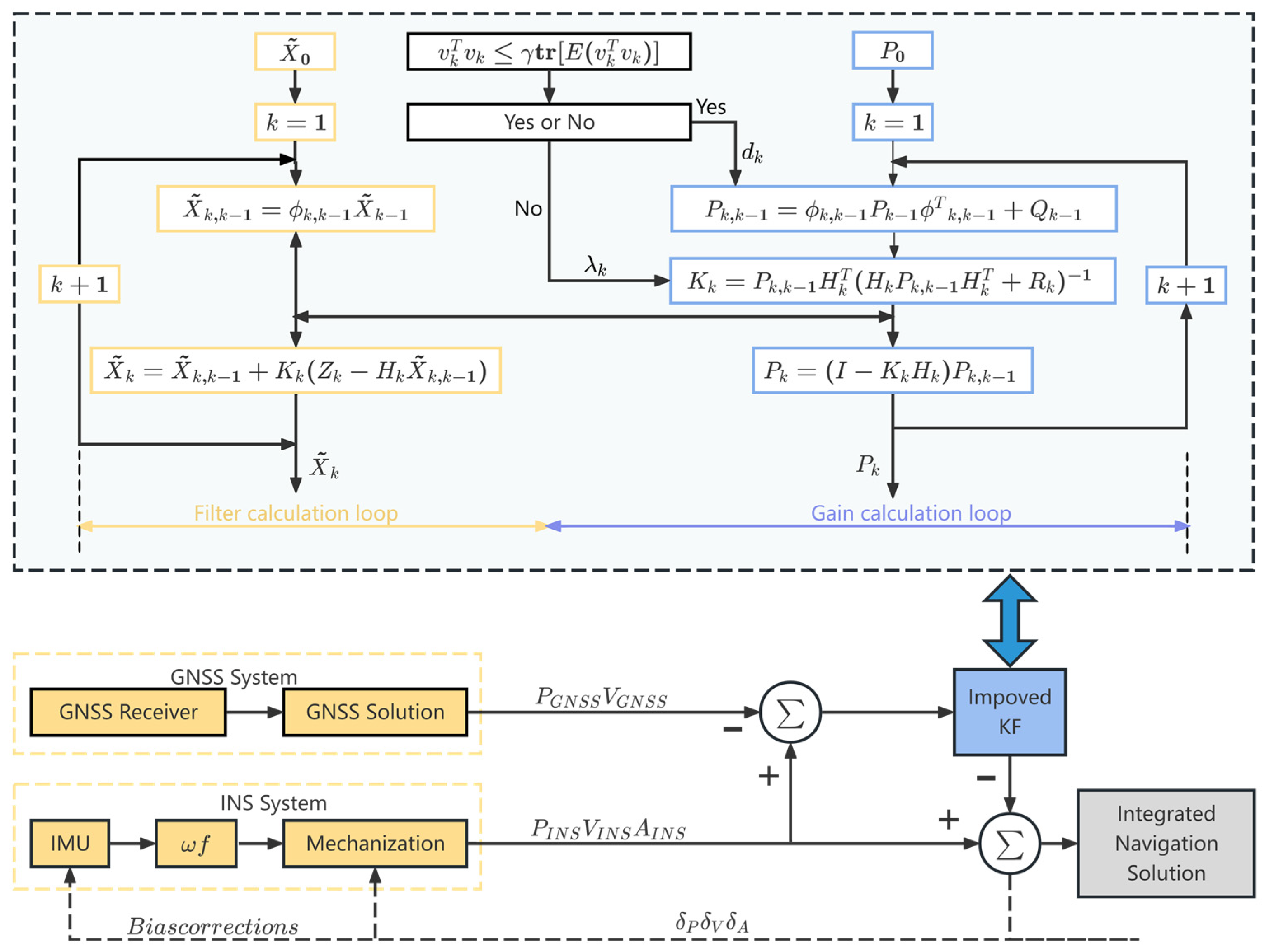
Given the uncertainty surrounding the covariance matrix of the predicted GNSS position, the conventional Kalman filter algorithm is not directly applicable. This study adopts an enhanced Kalman filtering approach, integrating the Sage–Husa adaptive filtering technique to dynamically estimate the statistical properties of pseudo-GNSS positions in real time, and coupling it with robust tracking Kalman filtering to derive the navigation solution for the integrated system during periods of GNSS signal loss.

The standard Kalman filter assumes that the process noise covariance and measurement noise covariance are known constants. However, in practical applications, these noise statistical characteristics may be unknown or vary over time. Sage–Husa adaptive filtering dynamically adjusts the filter parameters by online estimating the process noise covariance and measurement noise covariance, thereby improving filtering accuracy [26]. However, as the corrected measurement noise loses positive definiteness, filter divergence may occur, and the Sage–Husa adaptive filtering algorithm cannot fully guarantee the reliability, stability, and convergence of the system. In contrast, the strong tracking Kalman filter introduces a strong tracking factor, amplifying the predicted covariance, making the filter more sensitive to state mutations (e.g., target maneuvers or sudden acceleration) [27]. By combining Sage–Husa adaptive filtering and strong tracking Kalman filtering, a more robust adaptive strong tracking filter can be formed, which not only improves filtering accuracy but also enhances filter stability. This paper autonomously selects the filtering algorithm based on the filter’s convergence: Sage–Husa adaptive filtering is used when the filter is in a convergent state, and strong tracking Kalman filtering is adopted when the filter diverges.

2.2.1. Sage–Husa Adaptive Filtering

Sage–Husa adaptive filtering enables real-time estimation of the variance matrix of the pseudo-GNSS position. Its core lies in recursively estimating ${\tilde{R}}_k$ using the innovation and state estimation error. A fading factor (typically based on a forgetting factor 0 < b < 1) is introduced to weigh historical and current information, as shown in Equation (8):

$$\begin{array}{l}{d}_k={\displaystyle \frac{1-b}{1-b^{k+1}}},\hspace{1em}0<b<1\\ {\tilde{R}}_k=(1-d_{k-1}){\tilde{R}}_{k-1}+d_{k-1}\left(v_{k-1}{v}_{k-1}^T-H_k{P}_{k|k-1}{H}_k^T\right)\end{array}$$

(8)

2.2.2. Strong Tracking Kalman Filter

The strong tracking Kalman filter algorithm multiplies the state estimation covariance matrix in Equation (4) by a strong tracking factor, as shown in Equation (9):

$$P_{k,k-1}={\lambda }_k{\Phi }_{k,k-1}{P}_{k-1}{\Phi }_{k,k-1}^T+Q_{k-1}$$

(9)

The introduction of the strong tracking factor is the core of the strong tracking Kalman filter (STKF), which dynamically adjusts ${\lambda }_k$ by online estimation of the statistical characteristics of the residuals. The specific calculation formula is as follows:

$$r_k=\left\{\begin{array}{ll}{v}_k{v}_k^{\mathrm{T}}\hfill & (k=0)\hfill \\ {\displaystyle \frac{\rho r_{k-1}+v_k{v}_k^{\mathrm{T}}}{1+\rho }}\hfill & (k\ge 1)\hfill \end{array}\right.$$

(10)

$$C_k={\displaystyle \frac{\mathrm{Trace}[r_k-R_k-H{Q}_k{H}^T]}{\mathrm{Trace}[H{\Phi }_k{R}_k{\Phi }_k^T{H}^T]}}$$

(11)

$${\lambda }_k=\left\{\begin{array}{ll}{C}_k\hfill & (C_k>1)\hfill \\ 1\hfill & (C_k\le 1)\hfill \end{array}\right.$$

(12)

where $r_k$ is a recursive estimate of the innovation covariance, designed to capture abrupt system changes. $\rho$ (typically 0 ≤ $\rho$ ≤ 1) is the forgetting factor, which controls the relative weight of historical and current data in the residual covariance estimation. $C_k$ is an intermediate variable of the strong tracking factor, used to measure the deviation between the residual and the theoretical covariance. ${\lambda }_k$ enhances the filter’s ability to track abrupt state changes by amplifying the predicted covariance. Its core function is to dynamically adjust the filter’s level of trust: when a system mutation occurs, increasing ${\lambda }_k$ allows the filter to place more trust in the observation data and quickly correct the state estimate.

2.2.3. Implementation of Filter Convergence Assessment

When the filter diverges, the covariance matrix of the system error becomes unbounded (i.e., tends to infinity), indicating a significant discrepancy between the theoretical predicted error and the actual error. The actual estimated error of the innovation sequence is given by Equation (13):

$$v_k=Z_k-H_k{\tilde{X}}_{k,k-1}$$

(13)

The theoretical predicted covariance matrix of the innovation sequence (i.e., the expected value of $v_k^T{v}_k$) is as follows:

$$E(v_k{v}_k^{\mathrm{T}})=H_k{P}_{k,k-1}{H}_k^T+R_k$$

(14)

Thus, Equation (15) can be used to determine whether the filter converges. When Equation (15) holds, the filter is considered to be operating normally; otherwise, it is deemed divergent:

$$v_k{v}_k^{\mathrm{T}}\le \gamma \mathrm{tr}[E(v_k{v}_k^{\mathrm{T}})]$$

(15)

where tr denotes the matrix trace, and $\gamma$ ≥ 1 is an adjustable coefficient controlling the tolerance.

The above algorithm constitutes the improved Kalman filter algorithm proposed in this paper. The workflow of the loosely coupled navigation model and the improved Kalman filter algorithm is illustrated in Figure 1.

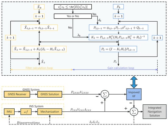
Figure 1. GNSS/INS loosely coupled structure and the process of robust Kalman filtering.

3. The Design of GNSS/INS Integrated Navigation Technology Based on CNN-BiLSTM-Attention

3.1. CNN-BiLSTM-Attention Model

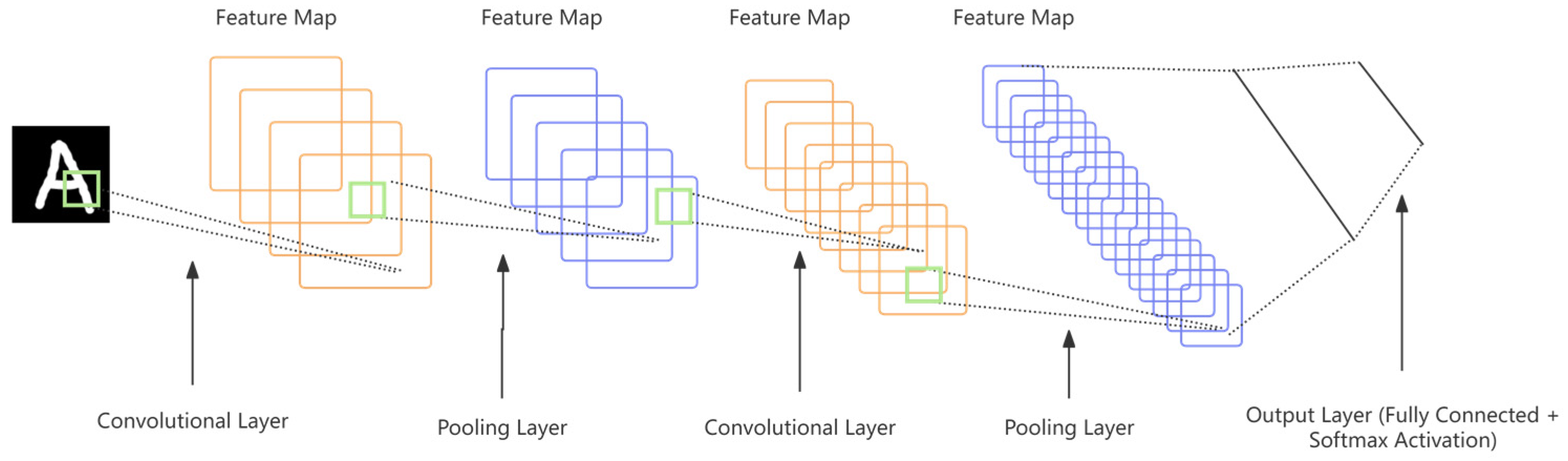
A Convolutional Neural Network (CNN) represents an advanced deep learning framework tailored for analyzing structured grid-like data, including images and time-series sequences [28]. The design of CNNs draws inspiration from the human visual system: when perceiving images, we often focus on local details (e.g., edges or textures) before integrating them into a comprehensive understanding. CNNs capture local patterns by sliding convolutional kernels over the input data, while leveraging parameter sharing and sparse connections to reduce computational complexity, making them particularly suitable for handling high-dimensional data.

Due to its specialized structure, CNNs can effectively explore relationships among various data types, extracting more significant features to enhance data quality, thus supporting improved prediction accuracy for GNSS displacement increments. The architecture of a Convolutional Neural Network (CNN) comprises convolutional, pooling, and fully connected layers, as depicted in Figure 2.

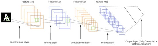
Figure 2. Structure of the CNN.

The convolutional layer, the core of a CNN, extracts local features by performing convolution operations between the input data and convolutional kernels (filters) [29]. The kernel slides over the input, computing the weighted sum of local regions, followed by an activation function (e.g., ReLU) to introduce nonlinearity. Subsequently, the pooling layer aggregates the convolutional features using techniques like max pooling or average pooling, effectively reducing data dimensionality. Finally, the fully connected layer transforms the features into a one-dimensional vector, further extracting feature representations.

It should be emphasized that CNNs cannot effectively handle time-series features [30]. To address this limitation, we introduce the Bidirectional Long Short-Term Memory (BiLSTM) model.

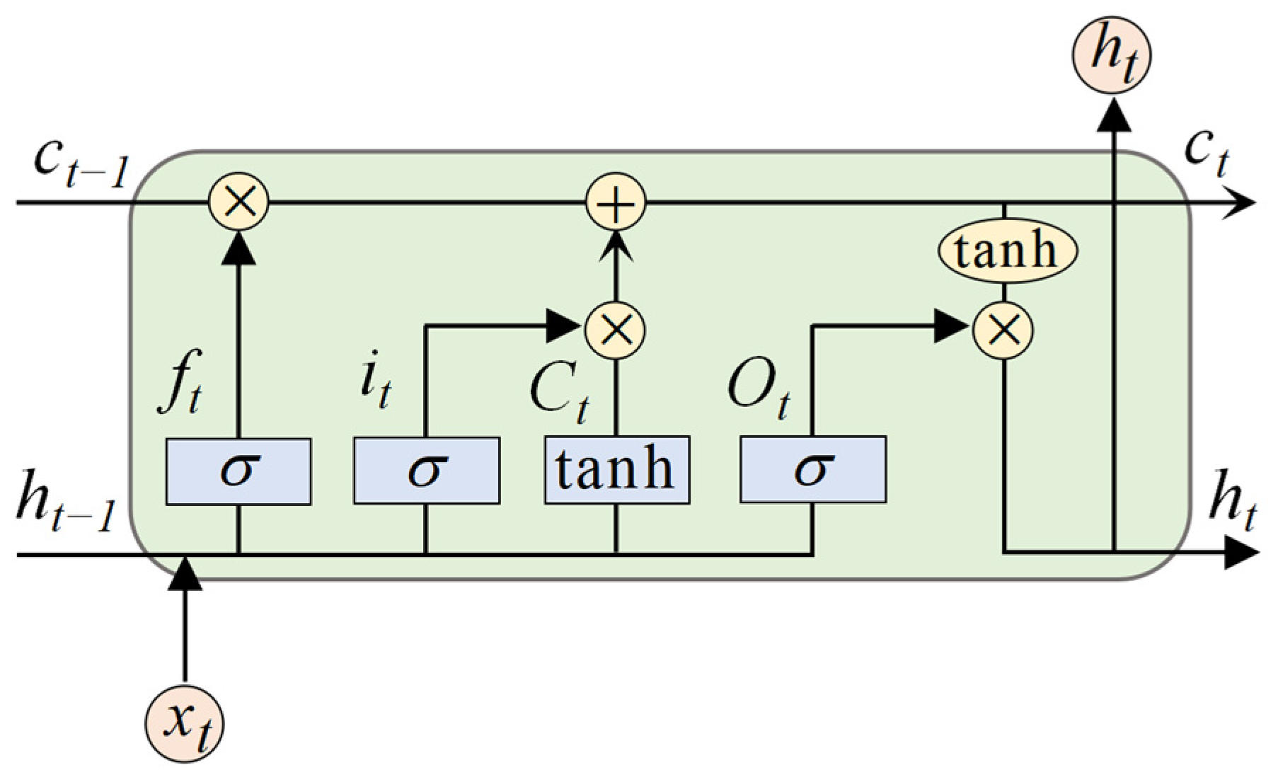
Long Short-Term Memory (LSTM), a specialized variant of Recurrent Neural Networks (RNNs), is designed to mitigate the challenges of gradient vanishing and explosion commonly faced by traditional RNNs when handling extended sequential data [31]. By incorporating a memory cell and a gate mechanism, LSTM enables the retention of essential information over prolonged periods while filtering out irrelevant data. The architecture of LSTM comprises three important gates—a forget gate, an input gate and an output gate—that collaboratively regulate the flow, retention, and updating of information, thereby facilitating effective modeling of time-series data [32]. Specifically, the forget gate determines which historical information to discard or retain for the subsequent unit, the input gate controls which new data should be stored in the memory cell, and the output gate governs the information to be passed to the next layer or time step [33]. The detailed structure of LSTM is illustrated in Figure 3, with its mathematical formulation provided as follows:

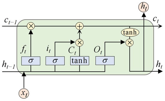
Figure 3. Structure of LSTM neural network.

Forget Gate:

$$f_t=\sigma (w_f\odot [h_{t-1},x_t]+b_f)$$

(16)

where $f_t$ is the forget gate output (a vector between 0 and 1), $\sigma$ is the sigmoid activation function, $w_f$ is the weight matrix, $b_f$ is the bias vector, and $\odot$ denotes element-wise multiplication.

Input Gate:

$$\begin{array}{l}{i}_t=\sigma (W_i\odot [h_{t-1},x_t]+b_i)\\ {\tilde{C}}_t=\tanh (W_c\odot [h_{t-1},x_t]+b_{\mathrm{c}})\\ C_t=f_t\odot C_{t-1}+i_t\odot {\tilde{C}}_t\end{array}$$

(17)

where $i_t$ is the input gate output, ${\tilde{C}}_t$ is the candidate cell state, and $C_t$ is the current cell state.

Output Gate:

$$\begin{array}{l}{O}_t=\sigma (W_o\odot [h_{t-1},x_t]+b_o)\\ h_t=O_t\odot \tanh (C_t)\end{array}$$

(18)

where $O_t$ is the output gate output, and $h_t$ is the hidden state.

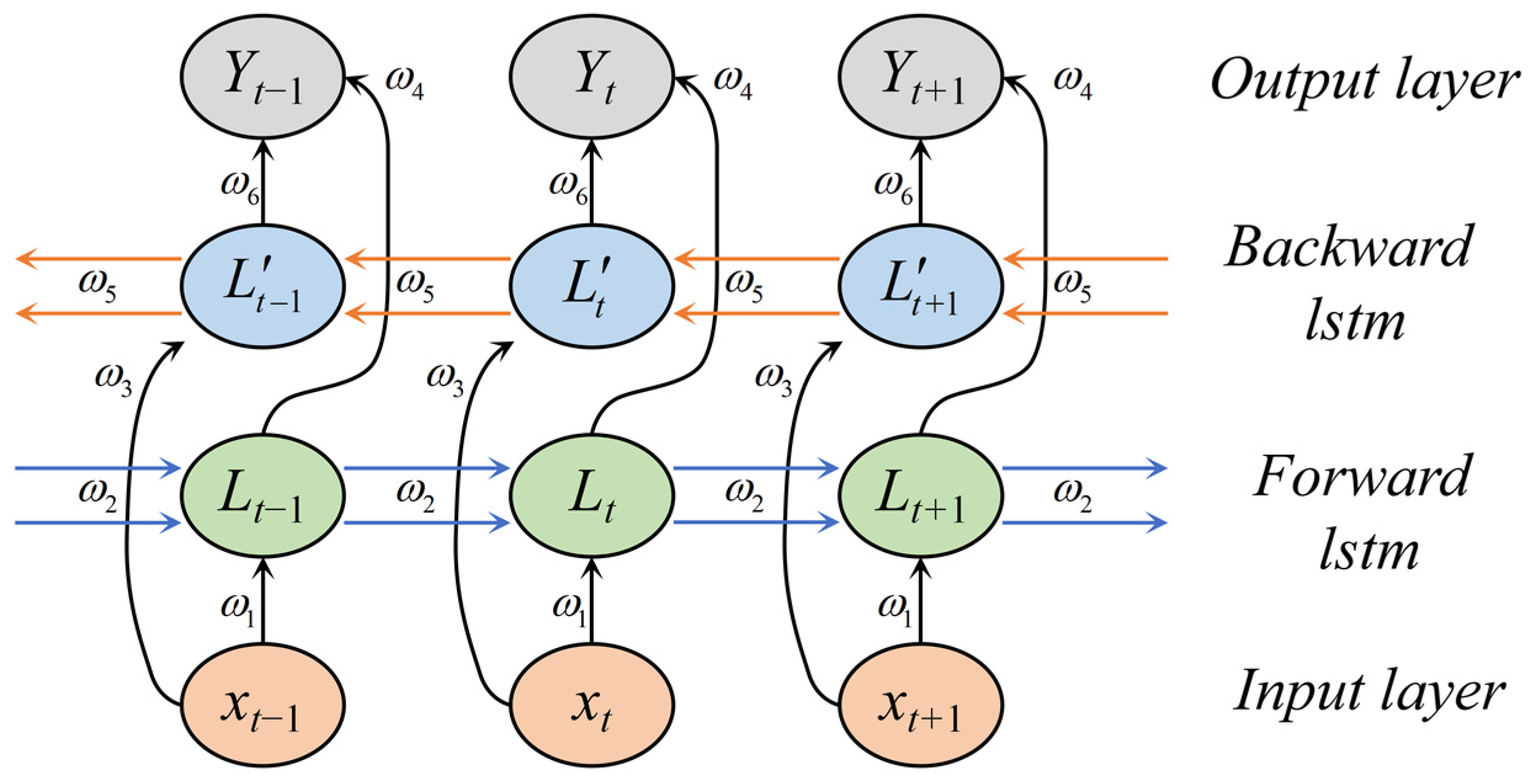
In a standard Long Short-Term Memory (LSTM) network, the state propagates unidirectionally, from past to present, capturing temporal dependencies in a single direction. However, in the context of vehicular navigation, the states of a vehicle exhibit strong temporal correlations not only with the preceding time steps but also with the subsequent ones, due to the continuous and dynamic nature of motion. To address this, this study leverages a Bidirectional Long Short-Term Memory (BiLSTM) framework to improve feature extraction capabilities. BiLSTM effectively captures the bidirectional temporal dependencies of vehicle states by integrating both a forward LSTM layer, which processes the sequence from past to present, and a backward LSTM layer, which processes it from future to past. The final output of the BiLSTM is determined by combining the hidden states of these two layers, as described in [34]. The detailed structure of the BiLSTM model is illustrated in Figure 4. Within this architecture, the hidden layers simultaneously update the states of the forward and backward LSTMs, enabling the model to produce a comprehensive representation of temporal features for GNSS/INS integrated navigation. The resulting output of the BiLSTM is formulated as follows:

$$L_t=f_1({\omega }_1{x}_t+{\omega }_2{A}_{t-1})$$

(19)

$$L_t^{\prime }=f_2({\omega }_3{x}_i+{\omega }_5{B}_{i+1})$$

(20)

$$Y_t=f_3({\omega }_4{L}_t+{\omega }_6{L}_t^{’})$$

(21)

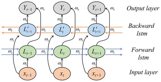
Figure 4. Structure of the BiLSTM.

Here, $f_1$, $f_2$, and $f_3$ represent the activation functions employed in each layer, and ${\omega }_{\mathrm{i}}$ denotes the weight matrices. The input vector at time step $\mathrm{t}$ is denoted as $x_{\mathrm{t}}$. The forward and backward hidden states of the bidirectional LSTM are represented by $L_t$ and $L_t^{\prime }$, respectively. The output vector $Y_t$ is obtained by concatenating the forward and backward hidden states.

The Attention Mechanism, a prevalent technique in deep learning, is designed to allow models to selectively concentrate on specific segments of the input sequence according to the demands of the task, instead of processing all information uniformly [35]. Its inspiration comes from human cognitive processes: when processing information, we often prioritize the parts most relevant to the current goal while ignoring secondary or irrelevant content. Its core lies in “adapting as needed”: adjusting the focus based on task objectives, which enhances both performance and model adaptability.

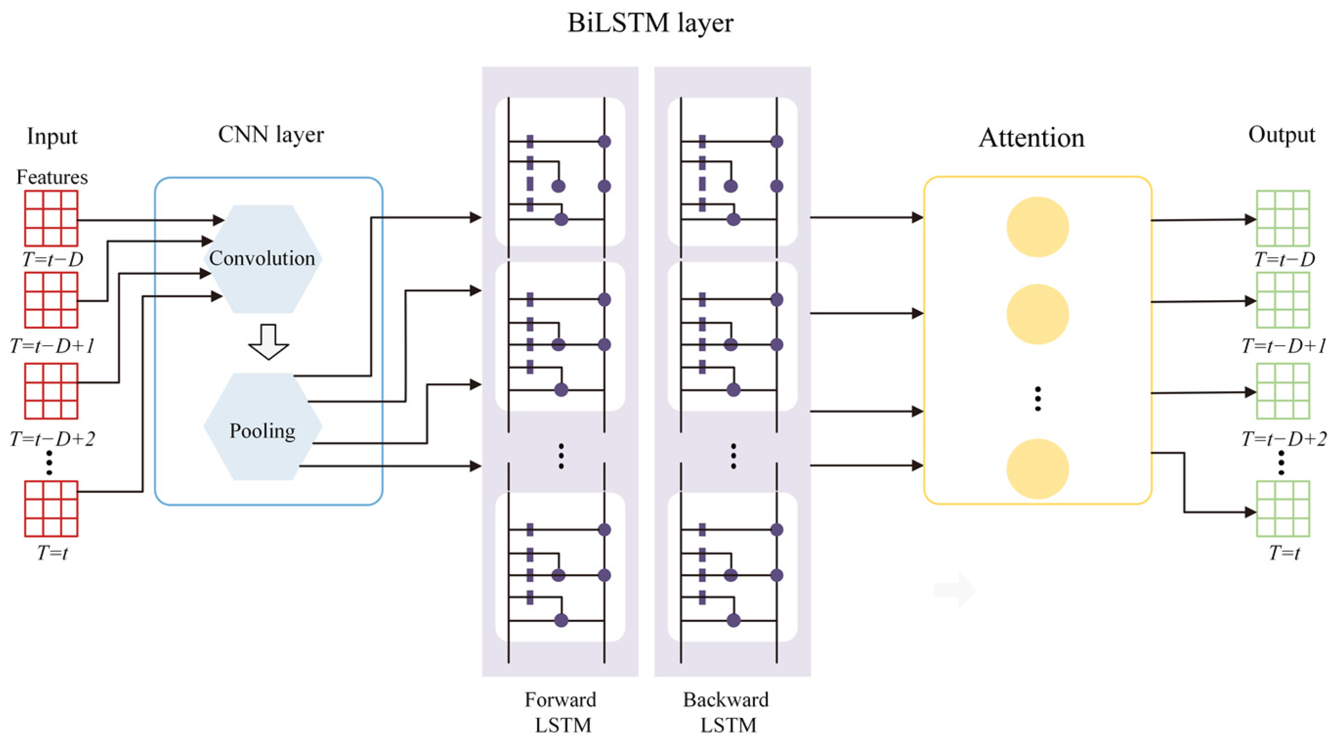
The architecture of the CNN-BiLSTM-Attention model is illustrated in Figure 5. A CNN framework, comprising two one-dimensional convolutional layers followed by a single pooling layer, is utilized to extract low-level features from the raw input data. The convolutional layers are designed to capture effective nonlinear local patterns, while the pooling layer subsequently reduces the dimensionality of the resulting feature maps, preserving key information and alleviating computational complexity [36]. The extracted local features are then fed into a BiLSTM module, which learns temporal dependencies within the sequence. The bidirectional nature of the BiLSTM, incorporating both forward and backward layers, allows the model to simultaneously process past and future contextual information, thereby generating a comprehensive global feature representation. These features are subsequently passed to an Attention Mechanism, which dynamically assigns weights to the BiLSTM outputs, emphasizing the time steps most relevant to the prediction task while mitigating the impact of less significant information. This approach enhances the model’s ability to uncover deep temporal relationships within the data, improving prediction accuracy. Finally, the output from the attention layer is processed through a fully connected layer to produce the final predictions of the CNN-BiLSTM-Attention model. The computational formulas for the attention layer are provided as follows:

$$Score=W_s\tanh (W_{q}X+W_{k}X+b)+b_s$$

(22)

$${\alpha }_i={\displaystyle \frac{\exp (scor{e}_i)}{{\displaystyle \sum _{j=1}^n\exp }(scor{e}_j)}}$$

(23)

$$c={\displaystyle \sum _{i=1}^n({\alpha }_i\cdot h_i)}$$

(24)

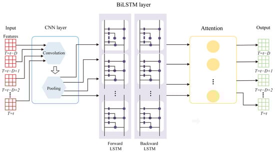
Figure 5. Structure of the CNN-BiLSTM-Attention.

First, compute the attention scores, which are the core of the attention module. Here, $W_s$ is the output score projection matrix, $W_q$ and $W_k$ are the query and key projection matrices, respectively, and $b$ and $b_s$ are bias terms. Next, apply a Softmax layer to the attention scores to normalize them and obtain the attention weight vector $a_{\mathrm{i}}$. Finally, use the attention weight vector $a_{\mathrm{i}}$ to compute a weighted sum over the hidden states $h_i$, producing the pseudo-GNSS signal at time $i$. In our experiments, the model’s hyperparameters were tuned through multiple trials to identify the optimal predictive configuration, as summarized in Table 1. The model is trained using the mean squared error (MSE) loss function, defined as follows:

$$L_{MSE}={\displaystyle \frac{1}{n}}{\displaystyle \sum _{i=1}^n{(y_i-{\widehat{y}}_i)}^2}$$

(25)

where ${\widehat{y}}_i$ is the model’s prediction and $y_i$ is the ground-truth GNSS increment.

Table 1. Hyperparameter setting.

Component	Parameter Description	Configured Values
CNN	Count of convolutional layers	2
	Size and count of convolution kernels	[1, 32], [1, 64]
	Count of pooling layers	2
	Pooling layer filter size	[1, 1]
BiLSTM	Number of hidden layers	2
	Neurons per hidden layer	[15, 10]
Attention	Total number of channels	32
Initial training	Maximum training iterations	100
	Batch size for training	16
	Learning rate	0.01
	Decay factor	0.1

3.2. Integrated Navigation System Assisted by CNN-BiLSTM-Attention

Compared to traditional filtering methods, deep learning approaches exhibit stronger adaptability, robustness, nonlinear modeling capabilities, and multi-source data fusion abilities in integrated navigation systems [37]. With the increase in computational power and data volume, deep learning is poised to further enhance the accuracy, efficiency, and reliability of integrated navigation systems, particularly in complex environments. The CNN-BiLSTM-Attention-based integrated navigation method proposed in this paper aims to establish a complex mapping relationship between vehicle motion observations and INS outputs. Depending on the output information of the constructed model, the models describing the relationship between INS outputs and GNSS information can be classified into three types. The first model outputs the difference between the position output by the GNSS and INS subsystems at the same time step. The second model outputs the state vector of the Kalman filter. The third model outputs the positional increment of the GNSS navigation information between two consecutive time steps. By comparing the outputs of the first, second, and third models, the third model is affected solely by the errors of the GNSS subsystem, reducing other mixed errors. Therefore, the third model is selected as the neural network training and prediction model. The positional increment can be expressed in the form of a double integral of the specific force equation:

$$\begin{array}{ll}\Delta P_{GNSS}& ={\displaystyle \iint {\stackrel{•}{V}}_n(t)dtdt}\\ & ={\displaystyle \iint \left(c_b^n{f}_{ib}^b(t)-\left(2{\omega }_{ie}^n(t)+{\omega }_{en}^n(t)\right)\times V^n(t)+g^n\right)}dtdt\end{array}$$

(26)

where

$$C_b^n=\left[\begin{array}{ccc}\cos \psi \cos \gamma +\sin \psi \sin \theta \sin \gamma & -\sin \psi \cos \gamma +\cos \psi \sin \theta \sin \gamma & -\cos \theta \sin \gamma \\ \sin \psi \cos \theta & \cos \psi \cos \theta & \sin \theta \\ \cos \psi \sin \gamma -\sin \psi \sin \theta \cos \gamma & -\sin \psi \sin \gamma +\cos \psi \sin \theta \cos \gamma & \cos \theta \cos \gamma \end{array}\right]$$

(27)

$${\dot{C}}_b^n=C_b^n\left({\omega }_b^n\times \right)=C_b^n\left({\omega }_{ib}^n\times \right)-\left({\omega }_{in}^n\times \right)C_b^n$$

(28)

$${\omega }_{en}^n={\left[{\displaystyle \frac{V_N}{R_M+h}},{\displaystyle \frac{V_E}{R_N+h}},{\displaystyle \frac{V_E}{R_N+h}}\tan L\right]}^T$$

(29)

From the above equation, it can be seen that the positional increment $\Delta P$ is related to the $C_b^n$, $f_{ib}^b$, ${\omega }_{ie}^n$, ${\omega }_{en}^n$, $V^n$, and $g^n$. Specifically, ${\omega }_{ie}^n$ and ${\omega }_{en}^n$ are primarily related to $V^n$, while $C_b^n$ is mainly influenced by the three attitude angles and ${\omega }_{ib}^b$; $g^n$ is primarily related to longitude and latitude. During vehicle operation, the roll and pitch angles are approximately 0 degrees, indicating that the main factors affecting the positional increment $\Delta P$ are the specific force, angular velocity, velocity, and heading angle. Therefore, the input and output values of this model are as follows:

$$\mathrm{Inputs}: [ f_{ib}^{\mathrm{b}} {\omega }_{ib}^b V^n \phi ]$$

(30)

$$\mathrm{Outputs}: [ \Delta P_{GNSS} ]$$

(31)

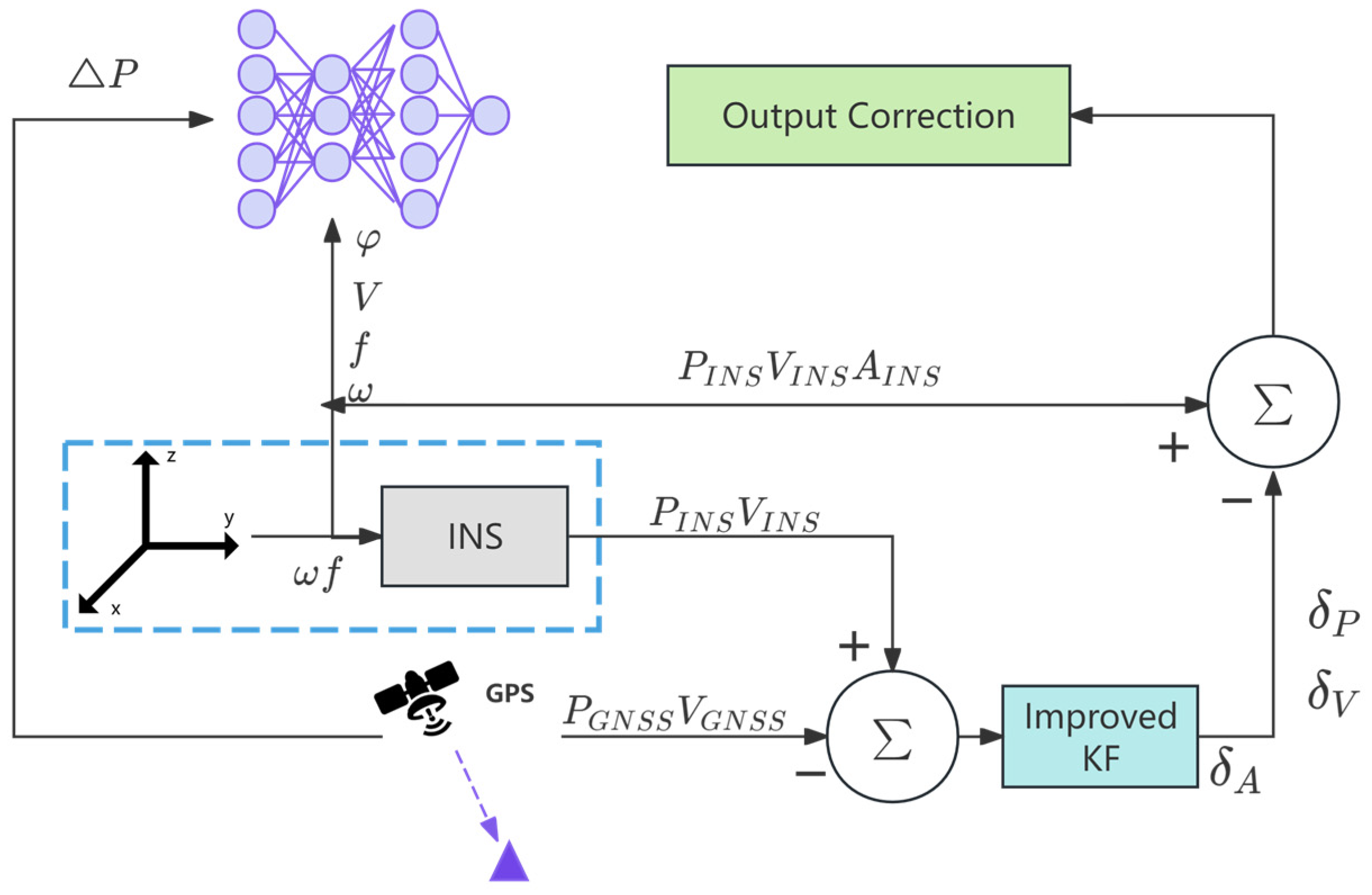
The CNN-BiLSTM-Attention-based integrated navigation error compensation method is divided into two modes. When GNSS is available, the differential GNSS navigation information and the information derived from INS mechanization can be fed into the improved Kalman filter to compute navigation solutions, which are then used for feedback correction of the INS. Additionally, this model takes IMU data (specific force, angular velocity, velocity, and heading angle) as inputs, with the GNSS increment at the corresponding time step serving as the target for neural network training, establishing the mapping relationship between inputs and targets. The specific workflow of model training is shown in Figure 6:

Figure 6. GNSS/INS integrated navigation during the model training phase.

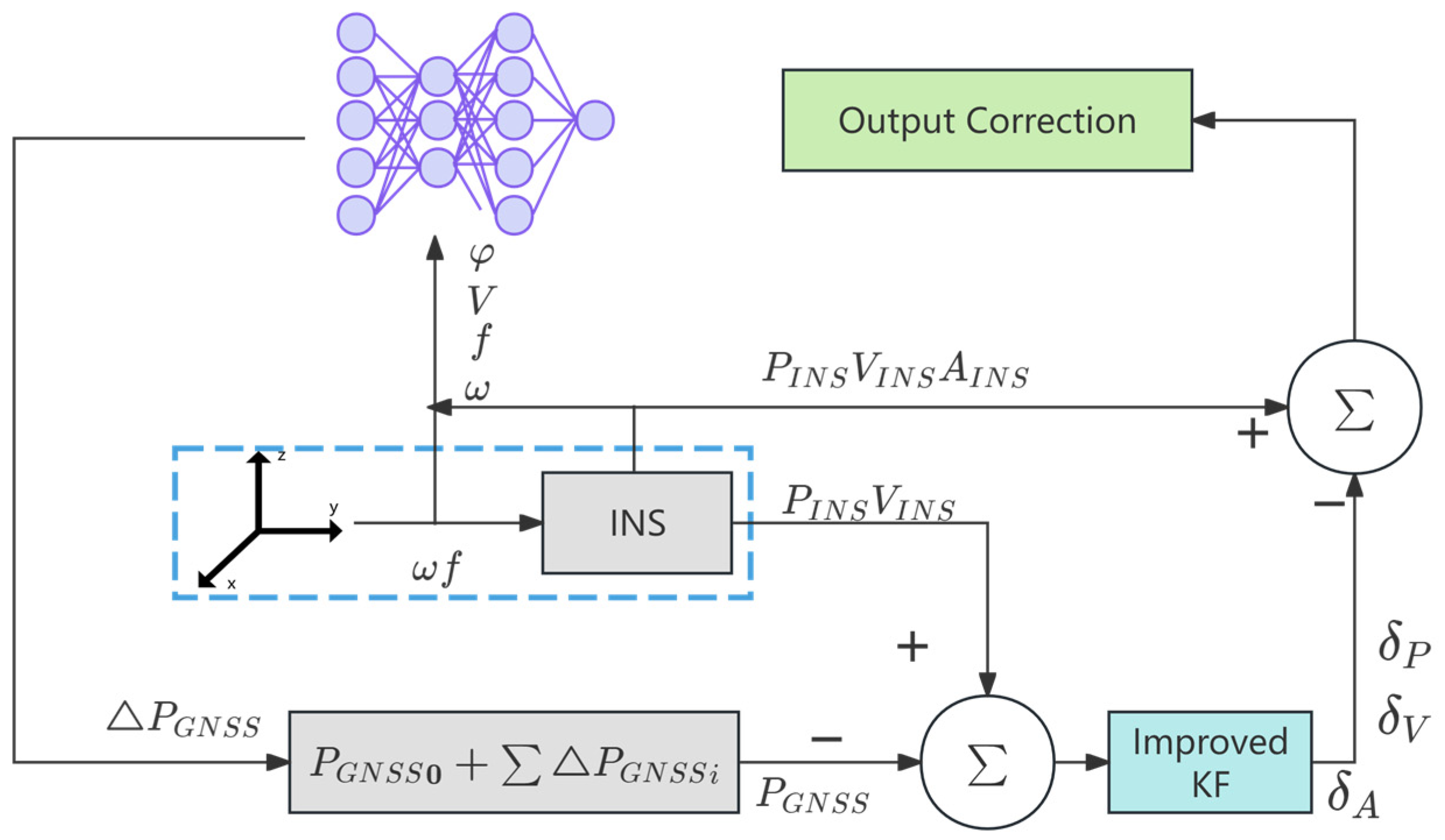
When GNSS signals are unavailable, GNSS cannot provide corresponding navigation information, and the integrated navigation system operates solely under the independent INS, leading to positioning errors that diverge over time. In this case, the pre-trained model is used to output pseudo-GNSS signals to correct the INS, as shown in Figure 7:

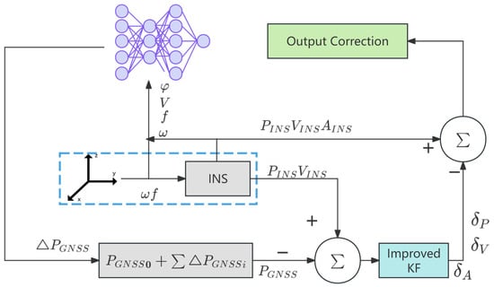
Figure 7. GNSS/INS integrated navigation during the model prediction phase.

Starting from the first epoch after the GNSS becomes unavailable, the positional increments $\Delta P_{GNSS}$ output by the model are accumulated to obtain the pseudo-GNSS position at each epoch. The formula is as follows:

$$P_{GNSS}^m=P_{GNS{S}_0}+{\displaystyle \sum _{i=0}^m\Delta P_{GNS{S}_i}}$$

(32)

where $P_{GNSS}^m$ represents the pseudo-GNSS position at time $m$, and $P_{GNS{S}_0}$ represents the vehicle’s position just before the GNSS signal outage. Finally, the pseudo-GNSS position information is integrated with the improved Kalman filter to achieve error compensation in the integrated navigation system.

4. Experiments and Analysis

To further validate the compensation performance of the proposed method for the GNSS/INS integrated navigation during GNSS signal outages, a real-vehicle experiment was conducted in Jiangsu Province, China. The experimental setup involved a SPAN-CPT inertial navigation system (IMU sampling rate: 100 Hz) and a Leica 1200 RTK-GNSS receiver (GNSS update rate: 1 Hz). The detailed specifications of the IMU sensor are provided in Table 2. In this study, the high-precision RTK-GNSS measurements were used as the reference trajectory, and the proposed algorithm was evaluated through post-processed navigation data during simulated GNSS outages.

Table 2. Specifications of the IMU sensor.

Sensor	Range	Bias	Random Walk	Scale Factor
Gyroscope	$\pm 375°\surd \mathrm{s}$	20°/h	$0.0667°/\surd \mathrm{h}$	1500 ppm
Accelerometer	$\pm 10 \mathrm{g}$	50 mg	$60 \mathsf{\mu }\mathrm{g}/\surd \mathrm{HZ}$	4000 ppm

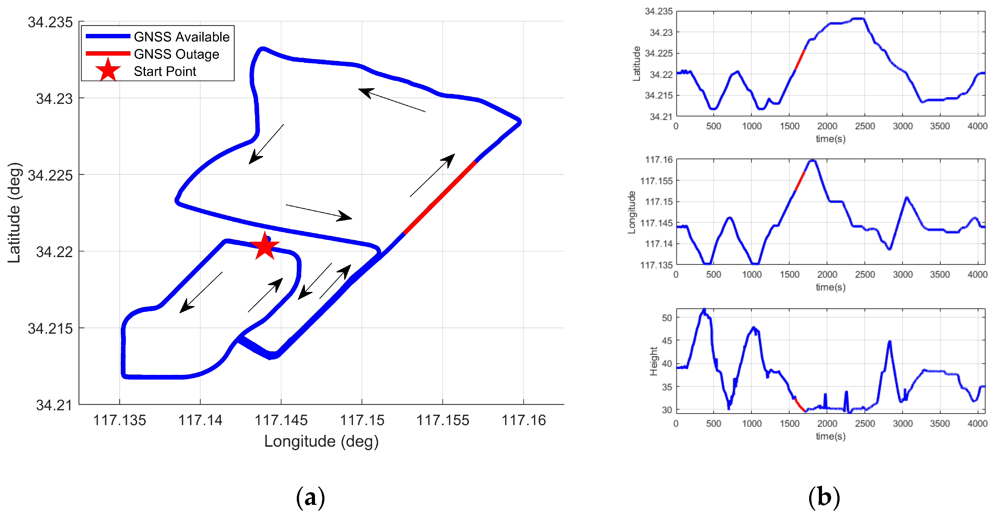
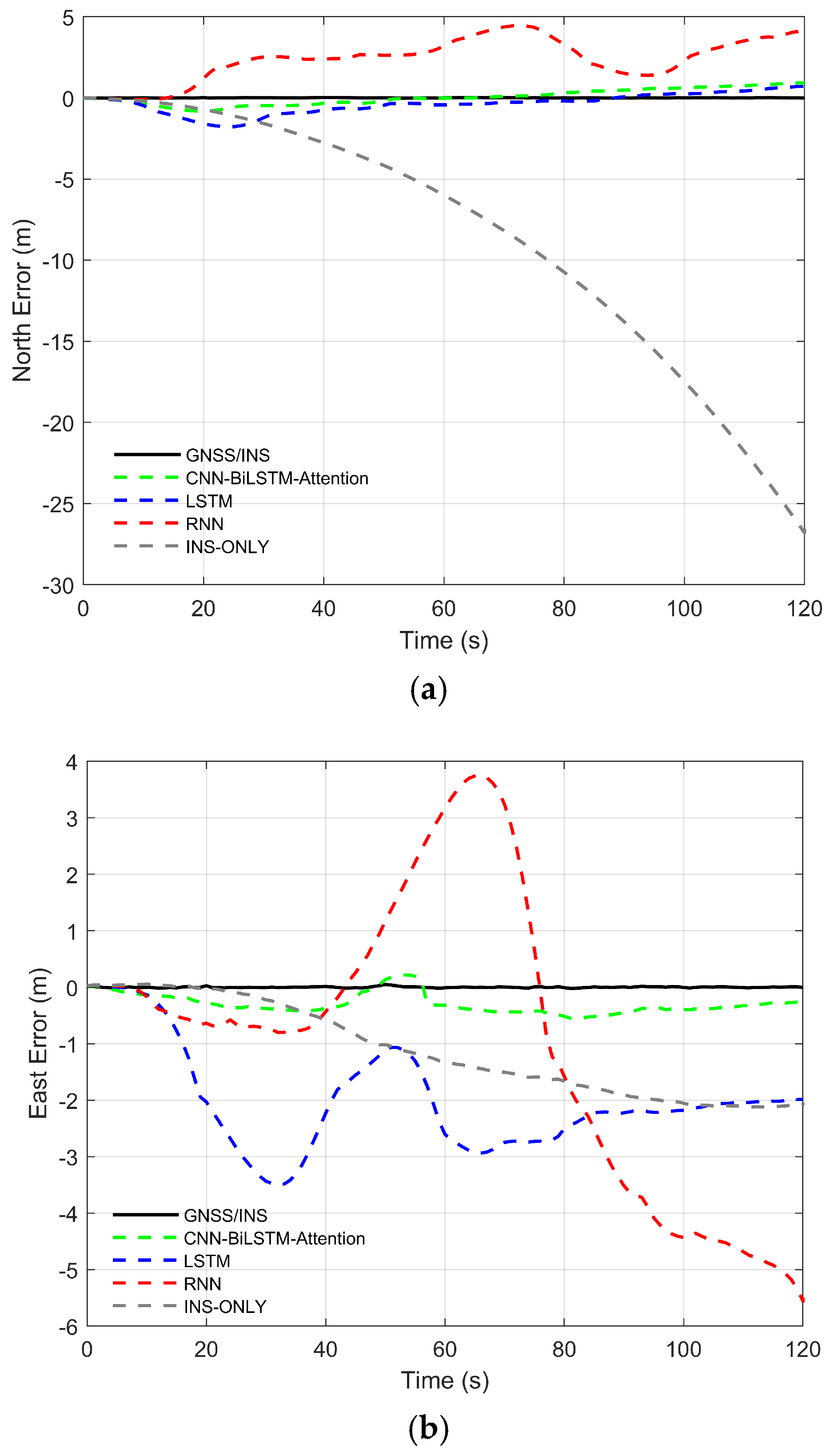
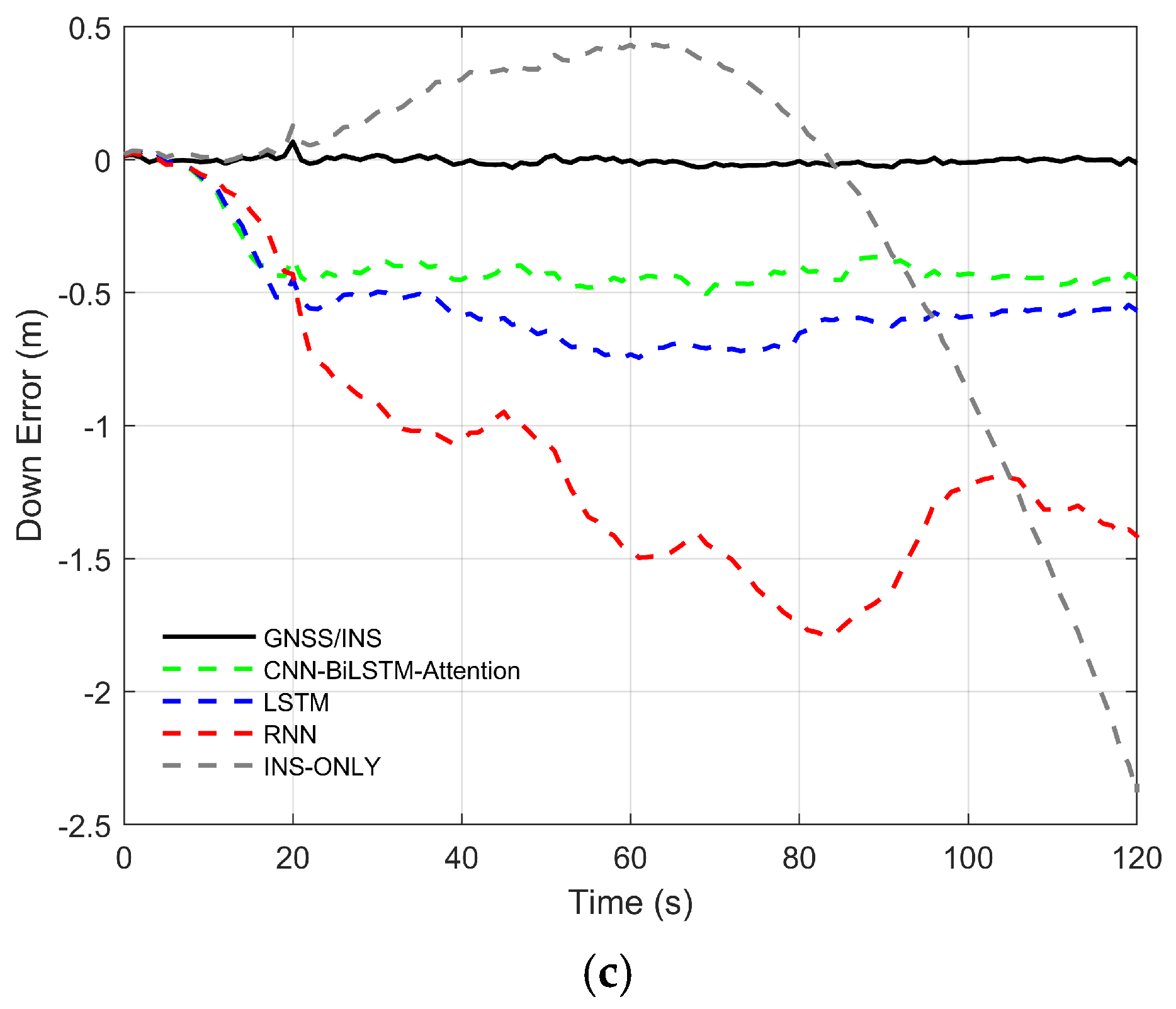
The vehicle traveled for a duration of one hour, and the driving trajectory is shown in Figure 8. To ensure the integrity of the experimental data, the experiment was conducted in an open area. In the later stage of the experiment, GNSS signal interruptions were simulated by manually removing GNSS observation data. In the figure, the blue solid line indicates the segments with available GNSS signals. The red solid line represents the prediction segment. A 100 s data segment starting from the 23rd minute was used as training data. The GNSS signal was cut off at the 26th minute and 20th second to simulate a 120 s GNSS outage. The red pentagram denotes the starting point of the vehicle. Figure 9 shows the positioning errors in the north, east, and down directions under different neural network algorithms.

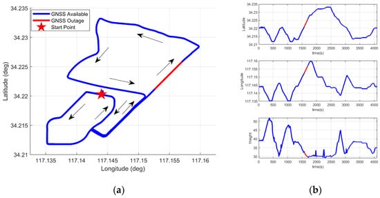
Figure 8. Vehicle test trajectory. (a) Vehicle reference trajectory. (b) Vehicle position trajectory.

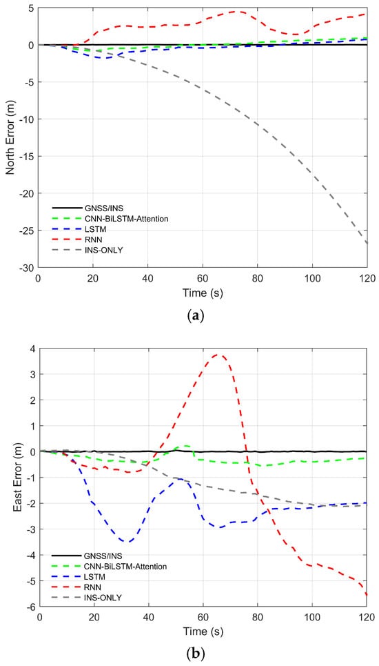
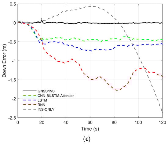
Figure 9. Positioning errors under different algorithms. (a) North error. (b) East error. (c) Down error.

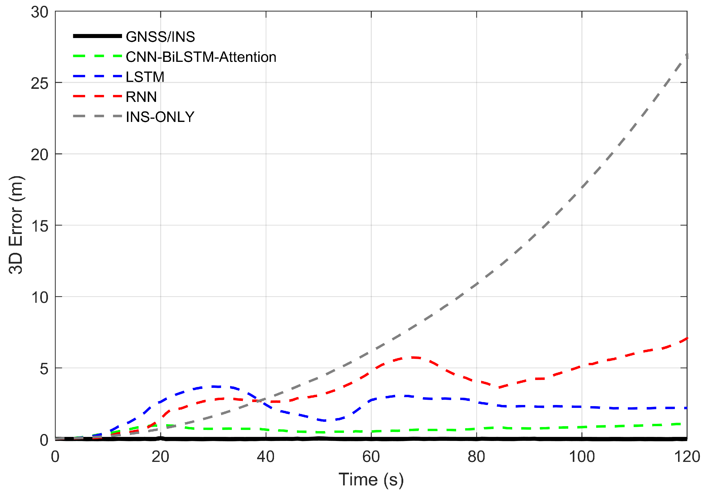
The three-dimensional positioning errors of the vehicle across various algorithms are presented in Figure 10. The corresponding computation formula is provided below:

$$\Delta P=\sqrt{\Delta N^2+\Delta E^2+\Delta D^2}$$

(33)

where $\Delta N$, $\Delta E$, $\Delta D$ and $\Delta P$ represent the north positioning error, east positioning error, altitude positioning error, and three-dimensional position error, respectively.

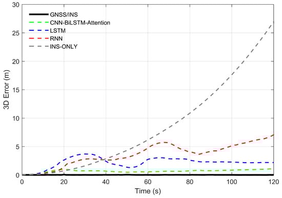
Figure 10. Vehicle positioning three-dimensional error.

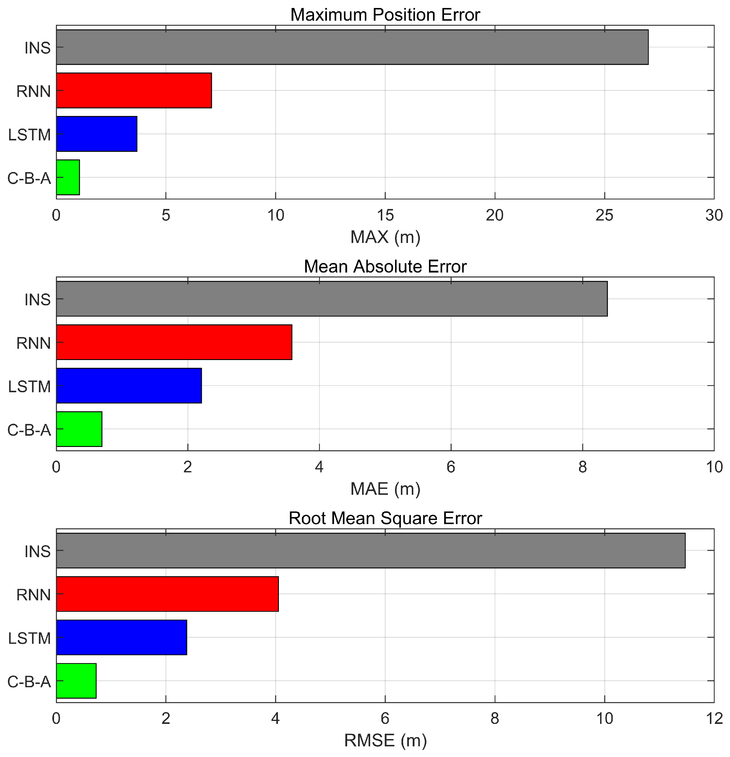
The maximum error (MAX), mean absolute error (MAE), and root mean square error (RMSE) are employed to evaluate the error compensation accuracy of different methods. The percentage error reduction of the proposed method relative to the standalone INS is also calculated. The statistical results are presented in Table 3, and the MAX, MAE, and RMSE in three-dimensional directions are shown in Figure 11. The calculation formulas are as follows:

$$\mathrm{MAX}={\max }_{i=1}^n\left|e_i\right|$$

(34)

$$\mathrm{MAE}={\displaystyle \frac{1}{n}}{\displaystyle \sum _{i=1}^n\left|e_i\right|}$$

(35)

$$\mathrm{RMSE}=\sqrt{{\displaystyle \frac{1}{n}}{\displaystyle \sum _{i=1}^n{e}_i^2}}$$

(36)

where $e_i$ represents the error of the i-th sample, and $n$ is the total number of samples.

Table 3. Statistical results of field experimental errors during GNSS outage.

Method and Index		INS	RNN	LSTM	CNN- BiLSTM- Attention	Percentage Reduction
North error (m)	MAX	26.8112	4.4577	1.7820	0.9282	96.54%
East error (m)		2.1216	5.5597	3.5069	0.5624	73.49%
Height error (m)		2.3810	1.7906	0.7455	0.5046	78.81%
3D error (m)		26.9968	7.0729	3.6818	1.0580	96.08%
North error (m)	MAE	8.2734	2.4095	0.5577	0.9282	95.00%
East error (m)		1.1092	2.1219	2.0000	0.3152	71.59%
Height error(m)		0.4680	1.0900	0.5381	0.3893	16.82%
3D error (m)		8.3736	3.5801	2.2055	0.6927	91.73%
North error (m)	RMSE	11.3666	2.7288	0.7182	0.4953	95.64%
East error (m)		1.3669	2.7420	2.1932	0.3423	74.95%
Height error(m)		0.7323	1.2034	0.5713	0.4083	44.24%
3D error (m)		11.4719	4.0513	2.3775	0.7275	93.66%

Figure 11. Evaluation metrics for three-dimensional position and orientation.

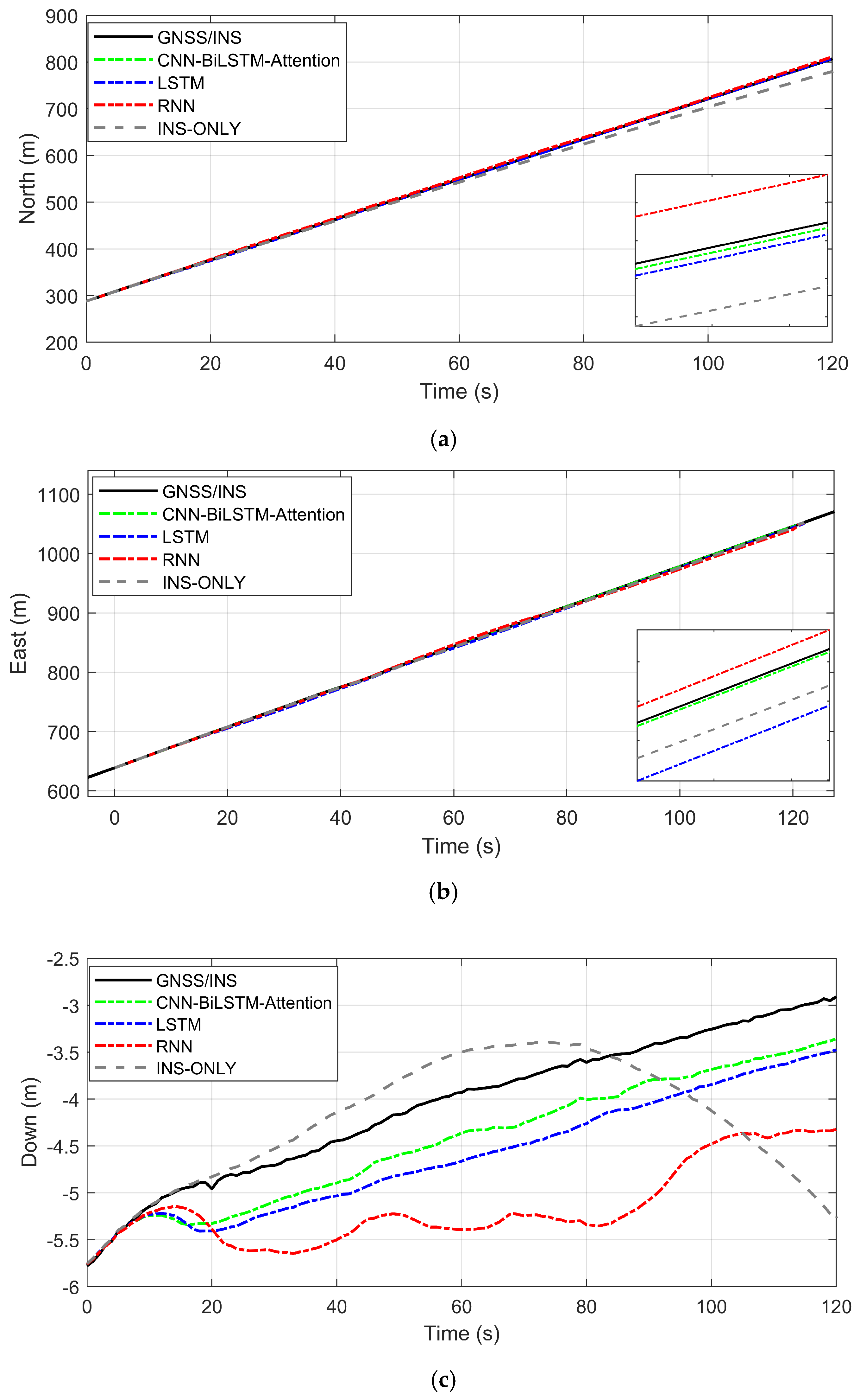
During GNSS outages, different neural network algorithms were used to predict the GNSS displacement increments, and the vehicle’s position was calculated using the improved Kalman filter. The position changes of the vehicle are shown in Figure 12, with the first epoch of the GNSS signal used as the reference point.

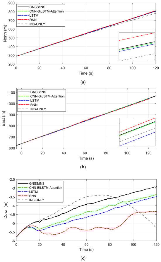
Figure 12. Position changes of vehicle under different algorithms during GNSS outages. (a) north direction; (b) east direction; (c) vertical direction.

From the above figures and tables, it can be observed that different methods exhibit varying compensation performance for the integrated navigation system during GNSS signal outages. The findings can be summarized as follows:

• During GNSS signal outages, the INS cannot integrate with the GNSS to correct system errors. This leads to rapid divergence of positioning errors in the standalone INS over time, with the divergence rate increasing progressively, failing to meet positioning requirements.
• Compared with the standalone INS, the introduction of RNN and LSTM for error compensation significantly improves positioning accuracy in the integrated navigation system. Among them, LSTM outperforms RNN, demonstrating its advantage in extracting temporal feature information. However, as the duration of GNSS signal outages increases, the positioning accuracy of RNN and LSTM in the east-direction error compensation gradually declines. In contrast, the proposed CNN-BiLSTM-Attention model remains unaffected by the prolonged outage duration, benefiting from both the bidirectional processing capability of BiLSTM and the dynamic focus of the Attention Mechanism. The synergy of these two components enables the model to comprehensively capture long-term dependencies and key information within the navigation data, thereby maintaining high positioning accuracy during GNSS signal outages.
• The CNN-BiLSTM-Attention method demonstrates the best compensation performance among the four methods. CNN extracts low-level spatial or temporal features from raw inputs, providing higher-quality input for the subsequent BiLSTM. BiLSTM combines forward and backward information flows, and the Attention Mechanism further optimizes the representation of sequential features by focusing on critical information. This model effectively suppresses the divergence of positioning errors, whether in the short or long term.
• In the north direction, the maximum error (MAX) of the INS reaches 26.8112 m, with MAE and RMSE being 8.2734 m and 11.3666 m, respectively. After introducing RNN, LSTM, and CNN-BiLSTM-Attention, the maximum errors are 4.4577 m, 1.7820 m, and 0.9282 m, respectively; the MAEs are 2.4095 m, 0.5577 m, and 0.4134 m; and the RMSEs are 2.7288 m, 0.7182 m, and 0.4953 m. Compared to INS, RNN, and LSTM, the positioning error of CNN-BiLSTM-Attention decreases by 95.00%, 82.84%, and 25.88% in MAE, and by 95.64%, 81.85%, and 31.04% in RMSE, respectively.
• In the east direction, the maximum error (MAX) of the INS reaches 2.1216 m, with MAE and RMSE being 1.1092 m and 1.3669 m, respectively. After introducing RNN, LSTM, and CNN-BiLSTM-Attention for error compensation, the maximum errors are 5.5597 m, 3.5069 m, and 0.5624 m, respectively; the MAEs are 2.1219 m, 2.0000 m, and 0.3152 m; and the RMSEs are 2.7420 m, 2.1932 m, and 0.3423 m. Compared to INS, RNN, and LSTM, the positioning error of CNN-BiLSTM-Attention decreases by 71.58%, 85.15%, and 84.24% in MAE, and by 74.96%, 87.52%, and 84.39% in RMSE, respectively.
• In the down direction, the maximum error (MAX) of INS reaches 2.3810 m, with MAE and RMSE being 0.4680 m and 0.7323 m, respectively. After introducing RNN, LSTM, and CNN-BiLSTM-Attention for error compensation, the maximum errors are 1.7906 m, 0.7455 m, and 0.5046 m, respectively; the MAEs are 1.0900 m, 0.5381 m, and 0.3893 m; and the RMSEs are 1.2034 m, 0.5713 m, and 0.4083 m. Compared to INS, RNN, and LSTM, the positioning error of CNN-BiLSTM-Attention decreases by 16.82%, 64.28%, and 27.65% in MAE, and by 44.24%, 66.07%, and 28.52% in RMSE, respectively.
• In the three-dimensional direction, the maximum error (MAX) of the INS is 26.9968 m, with MAE and RMSE being 8.3736 m and 11.4719 m, respectively. After introducing RNN, LSTM, and CNN-BiLSTM-Attention, the maximum errors are 7.0729 m, 3.6818 m, and 1.0580 m, respectively; the MAEs are 3.5801 m, 2.2055 m, and 0.6927 m; and the RMSEs are 4.0513 m, 2.3775 m, and 0.7275 m. In terms of MAE, compared to the other methods, the positioning accuracy of CNN-BiLSTM-Attention improves by 91.73%, 80.65%, and 68.59%, respectively. In terms of RMSE, the positioning accuracy of CNN-BiLSTM-Attention improves by 93.66%, 82.04%, and 69.40%, respectively. Overall, CNN-BiLSTM-Attention achieves the highest error compensation accuracy compared to the other methods.

Through the analysis of experimental results, compared to traditional neural networks, CNN-BiLSTM-Attention can better suppress the divergence of positioning errors, improving the vehicle’s positioning accuracy in the absence of GNSS signals.

5. Conclusions

This paper proposes an error compensation method for GNSS/INS integrated navigation based on CNN-BiLSTM-Attention to address positioning errors during GNSS signal outages. The feasibility and effectiveness of the proposed method were validated through real-vehicle experiments. The CNN-BiLSTM-Attention model integrates the strengths of CNN, BiLSTM, and the Attention Mechanism. Specifically, CNN extracts low-level spatial and temporal features from raw inputs, providing high-quality data for the subsequent BiLSTM. BiLSTM effectively models long-term dependencies within sequential data by integrating both forward and backward information streams. The Attention Mechanism further refines the output of BiLSTM by optimizing the representation of sequential features, enabling the model to dynamically focus on the most relevant information for the prediction task. This integration significantly enhances global dependency capture, dynamic feature selection, and computational efficiency.

When GNSS signals are available, a mapping relationship between IMU data and GNSS positional increments is established using the neural network model. During GNSS outages, the trained model generates pseudo-GNSS signals, which are combined with an improved Kalman filter to compensate for errors in the integrated navigation system, effectively suppressing the divergence of positioning errors. To evaluate the performance of the proposed method, real-vehicle experiments were conducted in Jiangsu Province, China. The experimental results demonstrate that, compared to standalone INS, RNN, and LSTM, the CNN-BiLSTM-Attention method improves positioning accuracy during GNSS outages by 91.06%, 86.58%, and 79.58%, respectively. These findings confirm that the proposed method can significantly mitigate the divergence of positioning errors in the absence of GNSS signals, thereby enhancing the positioning accuracy and robustness of the integrated navigation system. This approach provides reliable technical support for navigation tasks in challenging environments.

References

- Andrade, A.A.L. The Global Navigation Satellite System: Navigating into the New Millennium; Routledge: Oxfordshire, UK, 2017. [Google Scholar]
- Zidan, J.; Adegoke, E.I.; Kampert, E.; Birrell, S.A.; Ford, C.R.; Higgins, M.D. GNSS vulnerabilities and existing solutions: A review of the literature. IEEE Access 2020, 9, 153960–153976. [Google Scholar] [CrossRef]
- Elsanhoury, M.; Mäkelä, P.; Koljonen, J.; Välisuo, P.; Shamsuzzoha, A.; Mantere, T.; Elmusrati, M.; Kuusniemi, H. Precision positioning for smart logistics using ultra-wideband technology-based indoor navigation: A review. IEEE Access 2022, 10, 44413–44445. [Google Scholar] [CrossRef]
- Noureldin, A.; Karamat, T.B.; Eberts, M.D.; El-Shafie, A. Performance enhancement of MEMS-based INS/GPS integration for low-cost navigation applications. IEEE Trans. Veh. Technol. 2008, 58, 1077–1096. [Google Scholar] [CrossRef]
- Li, X.; Ge, M.; Dai, X.; Ren, X.; Fritsche, M.; Wickert, J.; Schuh, H. Accuracy and reliability of multi-GNSS real-time precise positioning: GPS, GLONASS, BeiDou, and Galileo. J. Geod. 2015, 89, 607–635. [Google Scholar] [CrossRef]
- Falco, G.; Pini, M.; Marucco, G. Loose and tight GNSS/INS integrations: Comparison of performance assessed in real urban scenarios. Sensors 2017, 17, 255. [Google Scholar] [CrossRef]
- Jing, H.; Gao, Y.; Shahbeigi, S.; Dianati, M. Integrity monitoring of GNSS/INS based positioning systems for autonomous vehicles: State-of-the-art and open challenges. IEEE Trans. Intell. Transp. Syst. 2022, 23, 14166–14187. [Google Scholar] [CrossRef]
- Zhuang, Y.; Sun, X.; Li, Y.; Huai, J.; Hua, L.; Yang, X.; Cao, X.; Zhang, P.; Cao, Y.; Qi, L.; et al. Multi-sensor integrated navigation/positioning systems using data fusion: From analytics-based to learning-based approaches. Inf. Fusion 2023, 95, 62–90. [Google Scholar] [CrossRef]
- Lu, Y.; Ma, H.; Smart, E.; Yu, H. Real-time performance-focused localization techniques for autonomous vehicle: A review. IEEE Trans. Intell. Transp. Syst. 2021, 23, 6082–6100. [Google Scholar] [CrossRef]
- Li, Q.; Li, R.; Ji, K.; Dai, W. Kalman filter and its application. In Proceedings of the 2015 8th International Conference on Intelligent Networks and Intelligent Systems (ICINIS), Tianjin, China, 1–3 November 2015. [Google Scholar]
- Li, M.; Mourikis, A.I. High-precision, consistent EKF-based visual-inertial odometry. Int. J. Robot. Res. 2013, 32, 690–711. [Google Scholar] [CrossRef]
- Soken, H.E.; Hajiyev, C.; Sakai, S.I. Robust Kalman filtering for small satellite attitude estimation in the presence of measurement faults. Eur. J. Control. 2014, 20, 64–72. [Google Scholar] [CrossRef]
- Hajiyev, C.; Soken, H.E. Robust adaptive Kalman filter for estimation of UAV dynamics in the presence of sensor/actuator faults. Aerosp. Sci. Technol. 2013, 28, 376–383. [Google Scholar] [CrossRef]
- Li, W.; Jia, Y. H-infinity filtering for a class of nonlinear discrete-time systems based on unscented transform. Signal Process. 2010, 90, 3301–3307. [Google Scholar] [CrossRef]
- Arasaratnam, I.; Haykin, S. Square-root quadrature Kalman filtering. IEEE Trans. Signal Process. 2008, 56, 2589–2593. [Google Scholar] [CrossRef]
- Jwo, D.J.; Biswal, A.; Mir, I.A. Artificial neural networks for navigation systems: A review of recent research. Appl. Sci. 2023, 13, 4475. [Google Scholar] [CrossRef]
- Sharaf, R.; Noureldin, A. Sensor integration for satellite-based vehicular navigation using neural networks. IEEE Trans. Neural Netw. 2007, 18, 589–594. [Google Scholar] [CrossRef]
- Tan, X.; Wang, J.; Han, H.; Yao, Y. Improved Neural Network-Assisted GPS/INS Integrated Navigation Algorithm. J. China Univ. Min. Technol. 2014, 43, 526–533. [Google Scholar]
- Gao, W.; Feng, X.; Zhu, D. Neural Network-Assisted Adaptive GPS/INS Integrated Navigation Algorithm. Acta Geod. Cartogr. Sin. 2007, 26, 64–67. [Google Scholar]
- Zhang, Y.; Wang, L. A hybrid intelligent algorithm DGP-MLP for GNSS/INS integration during GNSS outages. J. Navig. 2018, 72, 375–388. [Google Scholar] [CrossRef]
- Dai, H.F.; Bian, H.W.; Wang, R.Y.; Ma, H. An INS/GNSS integrated navigation in GNSS denied environment using recurrent neural network. Def. Technol. 2020, 16, 334–340. [Google Scholar] [CrossRef]
- Zhang, Y. A fusion methodology to bridge GPS outages for INS/GPS integrated navigation system. IEEE Access 2019, 7, 61296–61306. [Google Scholar] [CrossRef]
- Zhang, H.; Zhang, Q.; Shao, S.; Niu, T.; Yang, X. Attention-based LSTM network for rotatory machine remaining useful life prediction. IEEE Access 2020, 8, 132188–132199. [Google Scholar] [CrossRef]
- Simon, D. Kalman filtering. Embed. Syst. Program. 2001, 14, 72–79. [Google Scholar]
- Khodarahmi, M.; Vafa, M. A review on Kalman filter models. Arch. Comput. Methods Eng. 2023, 30, 727–747. [Google Scholar] [CrossRef]
- Narasimhappa, M.; Mahindrakar, A.D.; Guizilini, V.C.; Terra, M.H.; Sabat, S.L. MEMS-based IMU drift minimization: Sage Husa adaptive robust Kalman filtering. IEEE Sens. J. 2019, 20, 250–260. [Google Scholar] [CrossRef]
- Jwo, D.-J.; Wang, S.-H. Adaptive fuzzy strong tracking extended Kalman filtering for GPS navigation. IEEE Sens. J. 2007, 7, 778–789. [Google Scholar] [CrossRef]
- Park, W.B.; Chung, J.; Jung, J.; Sohn, K.; Singh, S.P.; Pyo, M.; Shin, N.; Sohn, K.S. Classification of crystal structure using a convolutional neural network. IUCrJ 2017, 4, 486–494. [Google Scholar] [CrossRef]
- Yang, A.; Yang, X.; Wu, W.; Liu, H.; Zhuansun, Y. Research on feature extraction of tumor image based on convolutional neural network. IEEE Access 2019, 7, 24204–24213. [Google Scholar] [CrossRef]
- Cui, Z.; Chen, W.; Chen, Y. Multi-scale convolutional neural networks for time series classification. arXiv 2016, arXiv:1603.06995. [Google Scholar]
- Salem, F.M. Recurrent Neural Networks; Springer International Publishing: Berlin/Heidelberg, Germany, 2022. [Google Scholar]
- Wang, J.; Sun, L.; Li, H.; Ding, R.; Chen, N. Prediction model of fouling thickness of heat exchanger based on TA-LSTM structure. Processes 2023, 11, 2594. [Google Scholar] [CrossRef]
- Greff, K.; Srivastava, R.K.; Koutník, J.; Steunebrink, B.R.; Schmidhuber, J. LSTM: A search space odyssey. IEEE Trans. Neural Netw. Learn. Syst. 2016, 28, 2222–2232. [Google Scholar] [CrossRef]
- Siami-Namini, S.; Tavakoli, N.; Namin, A.S. The performance of LSTM and BiLSTM in forecasting time series. In Proceedings of the 2019 IEEE International Conference on Big Data (Big Data), Los Angeles, CA, USA, 9–12 December 2019. [Google Scholar]
- Guo, M.-H.; Xu, T.-X.; Liu, J.-J.; Liu, Z.N.; Jiang, P.T.; Mu, T.J.; Zhang, S.-H.; Martin, R.R.; Cheng, M.-M.; HU, S.-M. Attention mechanisms in computer vision: A survey. Comput. Vis. Media 2022, 8, 331–368. [Google Scholar] [CrossRef]
- Liu, Y.; Pu, H.; Sun, D.-W. Efficient extraction of deep image features using convolutional neural network (CNN) for applications in detecting and analysing complex food matrices. Trends Food Sci. Technol. 2021, 113, 193–204. [Google Scholar] [CrossRef]
- Ye, X.; Song, F.; Zhang, Z.; Zeng, Q. A review of small UAV navigation system based on multisource sensor fusion. IEEE Sens. J. 2023, 23, 18926–18948. [Google Scholar] [CrossRef]
Disclaimer/Publisher’s Note: The statements, opinions and data contained in all publications are solely those of the individual author(s) and contributor(s) and not of MDPI and/or the editor(s). MDPI and/or the editor(s) disclaim responsibility for any injury to people or property resulting from any ideas, methods, instructions or products referred to in the content. |
© 2025 by the authors. Licensee MDPI, Basel, Switzerland. This article is an open access article distributed under the terms and conditions of the Creative Commons Attribution (CC BY) license (https://creativecommons.org/licenses/by/4.0/).