
Research on Full-Sky Star Identification Based on Spatial Projection and Reconfigurable Navigation Catalog


Abstract
:
1. Introduction
2. Principles and Methods
3. Detailed Program and Experimental Analysis
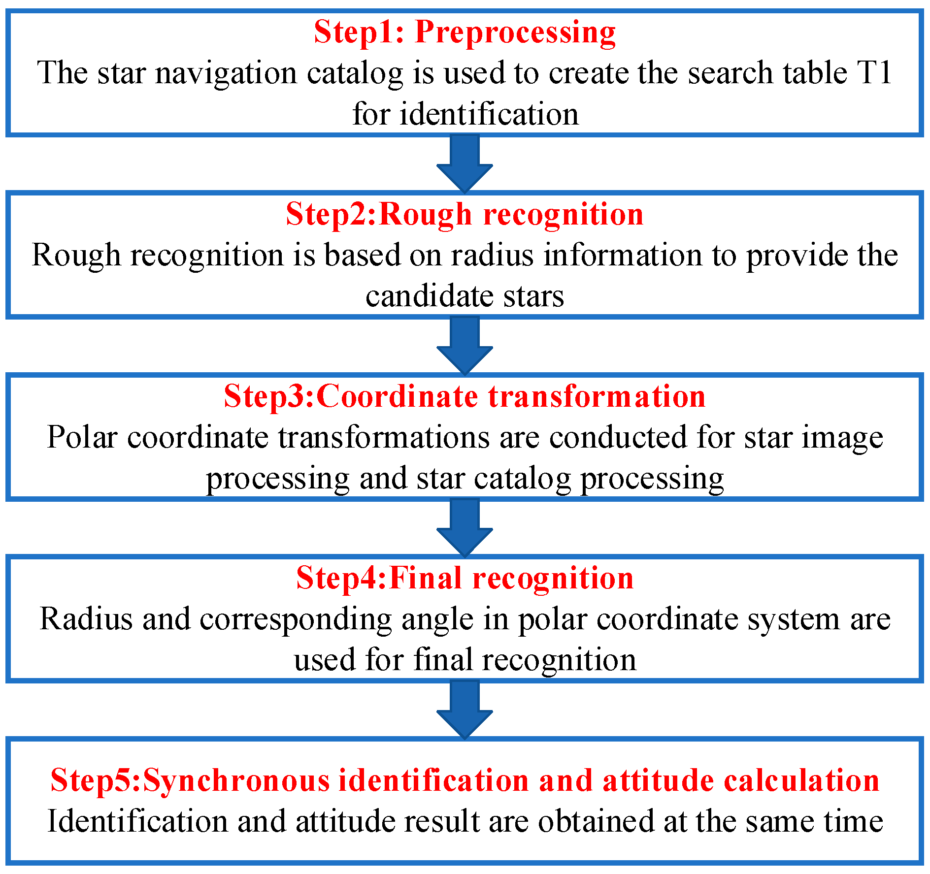
3.1. Star Identification Algorithm
3.2. Regression Verification
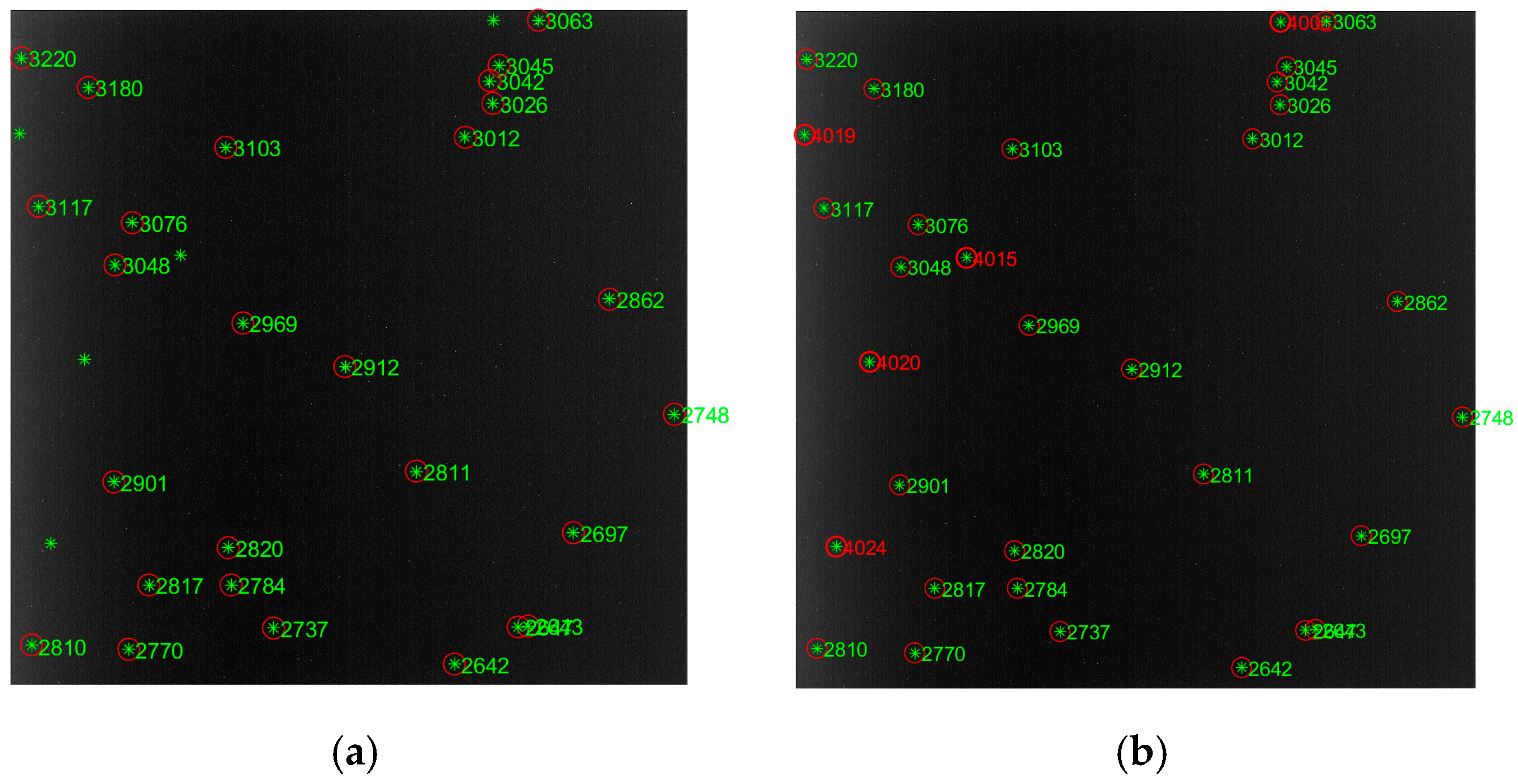
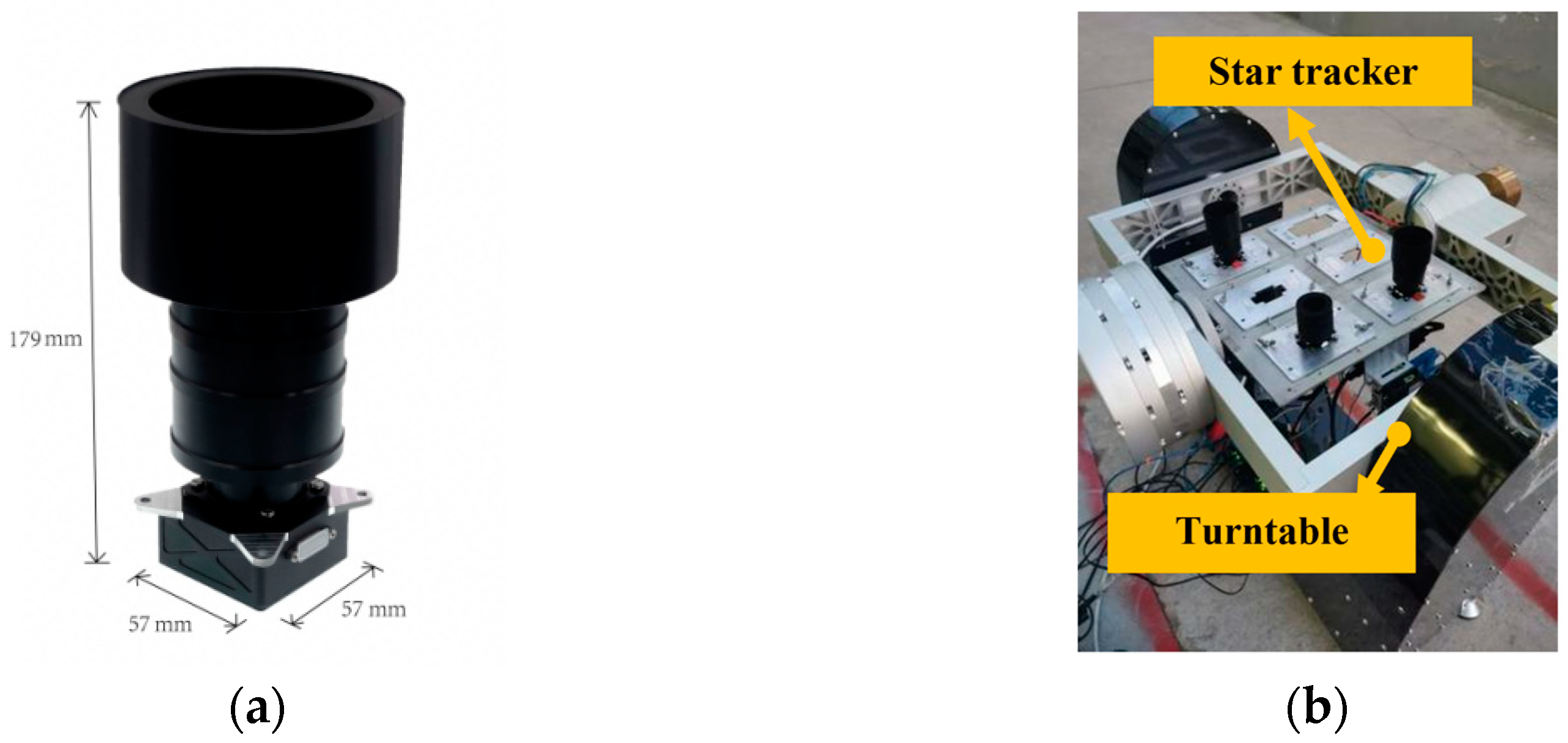
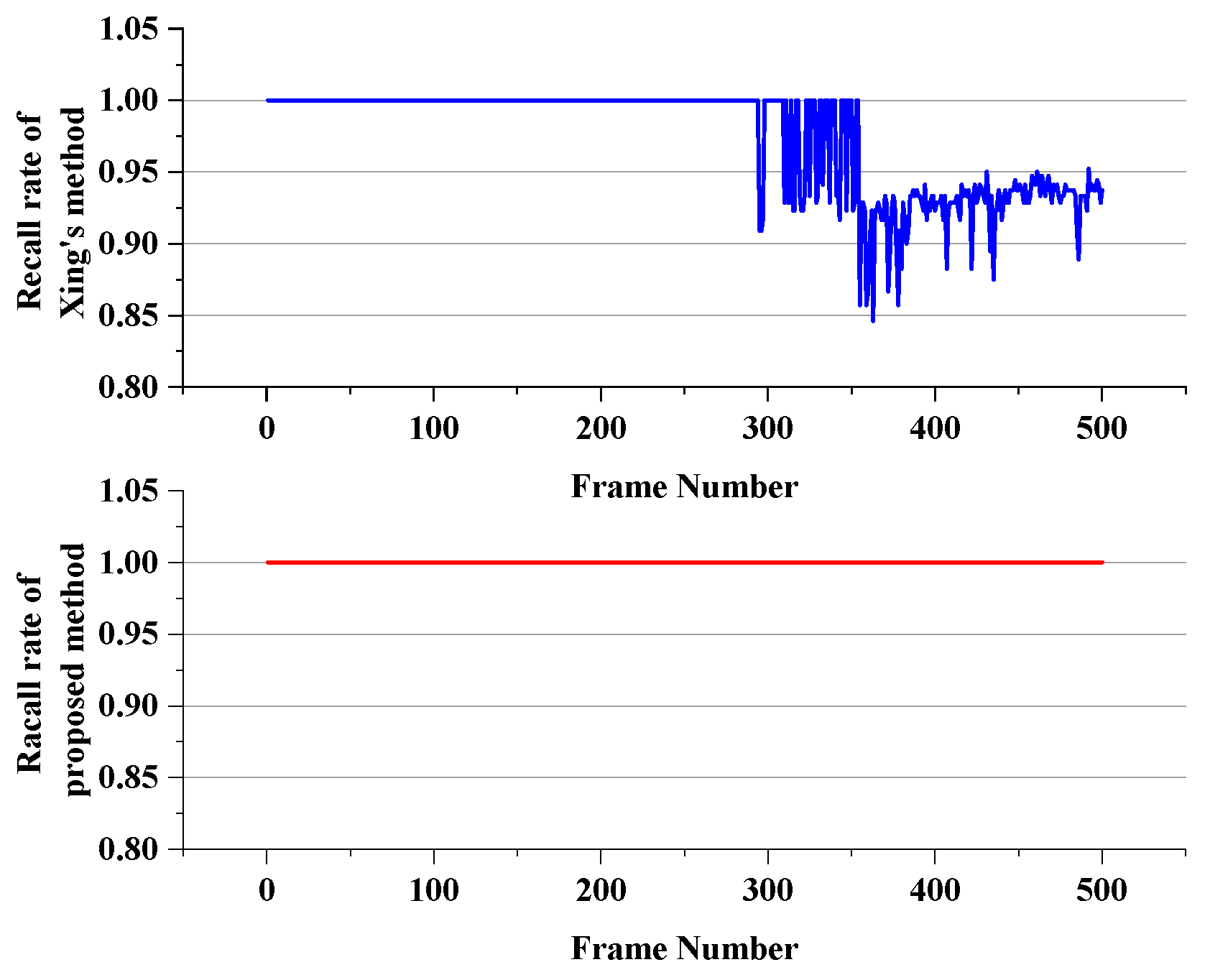
3.3. Experiment and Analysis with Interference
3.4. Reconstruction of the Navigation Catalog
4. Discussion
5. Conclusions
Author Contributions
Funding
Data Availability Statement
Acknowledgments
Conflicts of Interest
References
- Spratling, B.B., IV; Mortari, D. A survey on star identification algorithms. Algorithms 2009, 2, 93–107. [Google Scholar] [CrossRef]
- Sun, T.; Xing, F.; Bao, J.; Zhan, H.; Han, Y.; Wang, G.; Fu, S. Centroid determination based on energy flow information for moving dim point targets. Acta Astronaut. 2022, 192, 424–433. [Google Scholar] [CrossRef]
- Zhan, H.; Xing, F.; Bao, J.; Sun, T.; Chen, Z.; You, Z.; Yuan, L. Analyzing the effect of the intra-pixel position of small PSFs for optimizing the PL of optical subpixel localization. Engineering 2023, 27, 140–149. [Google Scholar] [CrossRef]
- Padgett, C.; Kreutz-Delgado, K.; Udomkesmalee, S. Evaluation of star identification techniques. J. Guid. Control Dyn. 1997, 20, 259–267. [Google Scholar] [CrossRef]
- Scholl, M. Star field identification algorithm. Opt. Lett. 1993, 18, 399–401. [Google Scholar] [CrossRef]
- Scholl, M. Experimental demonstration of a star field identification algorithm. Opt. Lett. 1993, 18, 402–404. [Google Scholar] [CrossRef]
- Scholl, M. Star field identification for autonomous attitude determination. J. Guid. Control Dyn. 1995, 18, 61–65. [Google Scholar] [CrossRef]
- Liebe, C.C. Pattern recognition of star constellations for spacecraft applications. IEEE Aerosp. Electron. Syst. Mag. 1992, 7, 34–41. [Google Scholar] [CrossRef]
- Kosik, J.C. Star pattern identification aboard an inertially stabilized aircraft. J. Guid. Control Dyn. 1991, 14, 230–235. [Google Scholar] [CrossRef]
- DeAntonio, L.; Udomkesmalee, S.; Alexander, J.; Blue, R.; Dennison, E.; Sevaston, G.; Scholl, M. Star-tracker based, all-sky, autonomous attitude determination. SPIE Proc. Space Guid. Control Track. 1993, 1949, 204–215. [Google Scholar]
- Mortari, D.; Samaan, M.A.; Bruccoleri, C.; Junkins, J.L. The pyramid star identification technique. Navigation 2004, 51, 171–183. [Google Scholar] [CrossRef]
- Liu, H.; Wei, X.; Li, J.; Wang, G. A star identification algorithm based on simplest general subgraph. Acta Astronaut. 2021, 183, 11–22. [Google Scholar] [CrossRef]
- Sun, Q.; Niu, Z.; Li, Y.; Wang, Z. A Robust High-Accuracy Star Map Matching Algorithm for Dense Star Scenes. Remote Sens. 2024, 16, 2035. [Google Scholar] [CrossRef]
- He, X.; Zhang, L.; He, J.; Mu, Z.; Lv, Z.; Wang, J. A Voting-Based Star Identification Algorithm Using a Partitioned Star Catalog. Appl. Sci. 2025, 15, 397. [Google Scholar] [CrossRef]
- Spratling, B.B.; Mortari, D. The K-Vector ND and its Application to Building a Non-Dimensional Star Identification Catalog. J. Astronaut. Sci. 2011, 58, 261–274. [Google Scholar] [CrossRef]
- Gerhard, J. A Geometric Hashing Technique for Star Pattern Recognition. Master’s Thesis, West Virginia University, Morgantown, WV, USA, 2016. [Google Scholar]
- Zhao, Y.; Wei, X.; Li, J.; Wang, G. Star identification algorithm based on K–L transformation and star walk formation. IEEE Sens. J. 2016, 16, 5202–5210. [Google Scholar] [CrossRef]
- Padgett, C.; Kreutz-Delgado, K. A grid algorithm for autonomous star identification. IEEE Trans. Aerosp. Electron. Syst. 1997, 33, 202–213. [Google Scholar] [CrossRef]
- Lee, H.; Bang, H. Star Pattern Identification Technique by Modified Grid Algorithm. IEEE Trans. Aerosp. Electron. Syst. 2007, 43, 1112–1116. [Google Scholar]
- Na, M.; Zheng, D.; Jia, P. Modified grid algorithm for noisy all-sky autonomous star identification. IEEE Trans. Aerosp. Electron. Syst. 2009, 45, 516–522. [Google Scholar] [CrossRef]
- Wang, T.; Wang, G.; Wei, X.; Li, Y. A star identification algorithm for rolling shutter exposure based on Hough transform. Chin. J. Aeronaut. 2024, 37, 319–330. [Google Scholar] [CrossRef]
- Silani, E.; Lovera, M. Star identification algorithms: Novel approach & comparison study. IEEE Trans. Aerosp. Electron. Syst. 2006, 42, 1275–1288. [Google Scholar]
- Yoon, H.; Lim, Y.; Bang, H. New star-pattern identification using a correlation approach for spacecraft attitude determination. J. Spacecraft Satell. 2011, 48, 182–186. [Google Scholar] [CrossRef]
- Sun, L.; Jiang, J.; Zhang, G.; Wei, X. A discrete HMM-based feature sequence model approach for star identification. IEEE Sens. J. 2016, 16, 931–940. [Google Scholar] [CrossRef]
- Wei, X.; Wen, D.; Song, Z.; Xi, J. Star identification algorithm based on oriented singular value feature and reliability evaluation method. Int. J. Aeronaut. Space Sci. 2019, 62, 265–274. [Google Scholar] [CrossRef]
- Kim, K. A New Star Identification Using Patterns in the Form of Gaussian Mixture Models. Adv. Space Res. 2024, 74, 319–331. [Google Scholar] [CrossRef]
- Zhang, G.; Wei, X.; Jiang, J. Full-sky autonomous star identification based on radial and cyclic features of star pattern. Image Vision Comput. 2008, 26, 891–897. [Google Scholar] [CrossRef]
- Wei, X.; Zhang, G.; Jiang, J. Star identification algorithm based on log-polar transform. J. Aerosp. Comput. Inf. Commun. 2009, 6, 483–490. [Google Scholar] [CrossRef]
- Fang, Y.; Jiang, J.; Zou, Y. A star identification algorithm based on geometric verification. In Proceedings of the 2020 2nd International Conference on Robotics, Intelligent Control and Artificial Intelligence, Shanghai, China, 17–19 October 2020. [Google Scholar] [CrossRef]
- Dai, Y.; Shi, C.; Ben, L.; Zhu, H.; Zhang, R.; Wu, S.; Shan, S.; Xu, Y.; Zhou, W. Star Identification Algorithm Based on Dynamic Distance Ratio Matching. Remote Sens. 2025, 17, 62. [Google Scholar] [CrossRef]
- Crain, T.; Bishop, R.; Ely, T. Event detection and identification during autonomous interplanetary navigation. AIAA J. 2000, 38, 62–69. [Google Scholar]
- Quan, W.; Fang, J. A star recognition method based on the adaptive ant colony algorithm for star sensors. Sensors 2010, 10, 1955–1966. [Google Scholar] [CrossRef]
- Ma, W.; Zhang, J.; Wu, Y.; Jiao, L.; Zhu, H.; Zhao, W. A Novel Two-Step Registration Method for Remote Sensing Images Based on Deep and Local Features. Remote Sens. 2019, 57, 4834–4843. [Google Scholar] [CrossRef]
- Li, Y.; Niu, Z.; Sun, Q.; Xiao, H.; Li, H. BSC-Net: Background Suppression Algorithm for Stray Lights in Star Images. Remote Sens. 2022, 14, 4852. [Google Scholar] [CrossRef]
- Liu, L.; Niu, Z.; Li, Y.; Sun, Q. Multi-Level Convolutional Network for Ground-Based Star Image Enhancement. Remote Sens. 2023, 15, 3292. [Google Scholar] [CrossRef]
- Xing, F.; You, Z.; Dong, Y. A rapid star identification algorithm based-on navigation star domain and K vector. J. Astronaut. 2010, 31, 2302–2308. [Google Scholar]
- Sun, Q.; Liu, L.; Niu, Z.; Li, Y.; Zhang, J.; Wang, Z. A Practical Star Image Registration Algorithm Using Radial Module and Rotation Angle Features. Remote Sens. 2023, 15, 5146. [Google Scholar] [CrossRef]


| Parameters | Value |
|---|---|
| Focal length (mm) | 49.74 |
| Position of principal point (mm) | (7.583, 7.584) |
| Image plane size (pixels × pixels) | 1024 × 1024 |
| FOV (deg) | 17 × 17 |
| Serial Number of the Main Star in the Star Catalog | X in the Celestial Coordinate System | Y in the Celestial Coordinate System | Z in the Celestial Coordinate System | Magnitude |
|---|---|---|---|---|
| 1 | 0.013361 | −0.012375 | −0.999834 | 5.32 |
| 2 | 0.009891 | −0.040586 | −0.999127 | 4.73 |
| … | … | … | … | … |
| 4000 | 0.010127 | 0.010127 | 0.010127 | 1.73 |
| Serial Number of the Main Star in the Star Catalog | Number of Stars Around the Main Star | Serial Number of Selected Neighboring Star 1 in the Catalog | Serial Number of Selected Neighboring Star 2 in the Catalog | Serial Number of Selected Neighboring Star 3 in the Catalog | … |
|---|---|---|---|---|---|
| 1 | 43 | 2 | 3 | 4 | … |
| 2 | 56 | 1 | 3 | 4 | … |
| … | … | … | … | … | … |
| 4000 | 39 | 3961 | 3962 | 3963 | … |
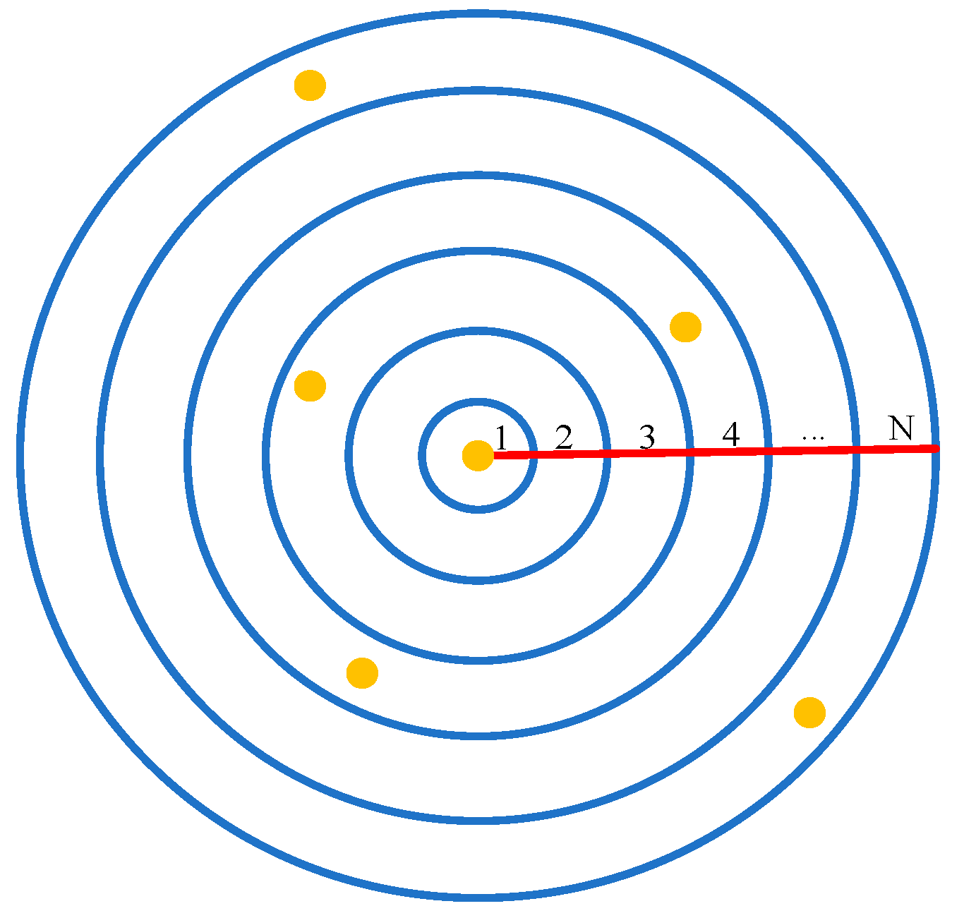
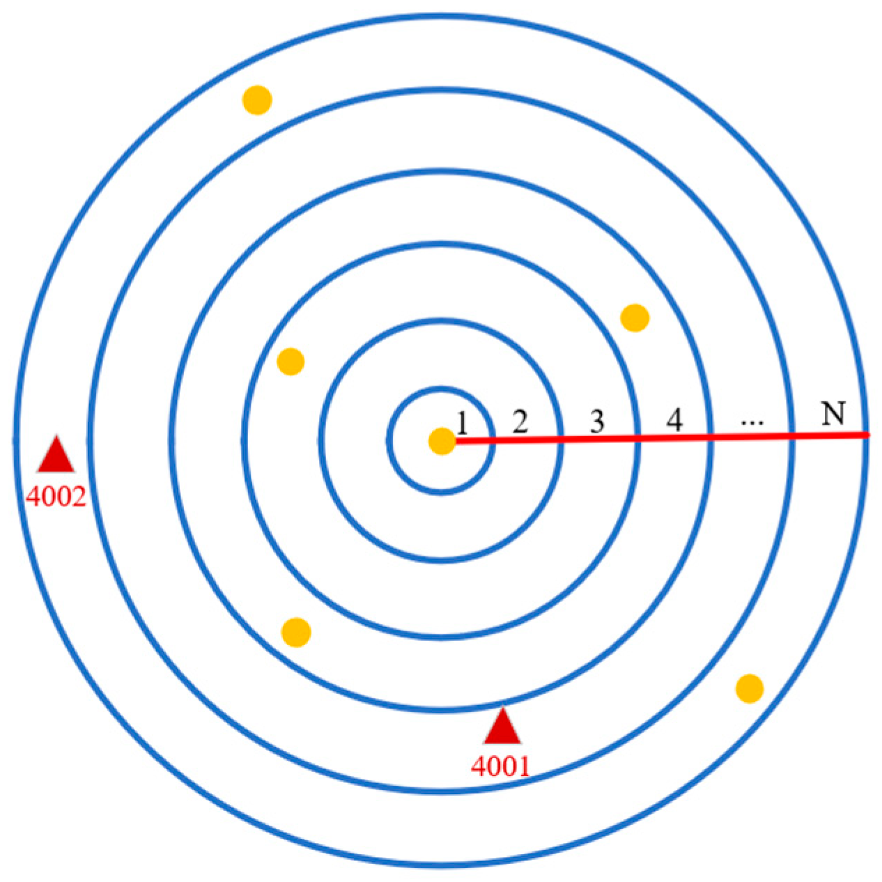
| Quantization Separated by Radius | Number of Stars Within the Radius Range |
|---|---|
| 1 | 0 |
| 2 | 0 |
| 3 | 1 |
| 4 | 2 |
| … | … |
| N | 2 |
| Serial Number of the Main Star in the Star Catalog | BP | BS | |||
|---|---|---|---|---|---|
| Number of Stars Around the Main Star | Serial Number of Selected Neighboring Star 1 in the Catalog | Serial Number of Selected Neighboring Star 2 in the Catalog | … | Serial Number of Selected Neighboring Star 3 in the Catalog | |
| 1 | 0 | 0 | 1 | … | 1 |
| 2 | 0 | 1 | 0 | … | 0 |
| 3 | 1 | 1 | 0 | … | 0 |
| 4 | 2 | 2 | 1 | … | 0 |
| … | … | … | … | … | … |
| N | 2 | 3 | 0 | … | 1 |
| Similarity | high | low | … | low | |
| MarkPos | MarkSelect | Result of Subtraction (°) | Flag | Identified Star Serial Number | ||
|---|---|---|---|---|---|---|
| (pixel) | (°) | (pixel) | (°) | |||
| 478.669 | 54.852 | 480.782 | 28.280 | 26.57 | 1 | 2643 |
| 478.669 | 54.852 | 473.539 | 29.835 | 25.02 | 0 | / |
| 478.669 | 54.852 | 479.881 | 43.264 | 11.59 | 0 | / |
| 191.941 | 55.585 | 191.827 | 29.085 | 26.50 | 1 | 2811 |
| 371.228 | 117.583 | 372.755 | 90.968 | 26.61 | 1 | 2784 |
| 374.100 | 120.584 | 372.755 | 90.968 | 29.62 | 0 | / |
| 374.100 | 120.584 | 377.643 | 215.005 | −94.42 | 0 | / |
| 442.825 | 131.990 | 444.105 | 105.361 | 26.63 | 1 | 2817 |
| … | … | … | … | … | … | … |
| Parameters | Value |
|---|---|
| Focal length (mm) | 18.50 |
| Position of principal point (mm) | (3.101, 2.496) |
| Image plane size (pixels × pixels) | 1040 × 1292 |
| FOV (deg) | 15 × 19 |
| Serial Number of the Main Star in the Star Catalog | Number of Stars Around the Main Star | Serial Number of Selected Neighboring Stars in the Catalog | ||||||
| 1 | 43 (44) | 2 | 3 | 4 | … | 4001 | … | … |
| 2 | 56 (58) | 1 | 3 | 4 | … | 4001 | 4002 | … |
| 3 | 57 (59) | 1 | 2 | 6 | … | 4001 | 4002 | … |
| … | … | … | … | … | … | … | … | … |
| 4000 | 39 | 3961 | 3962 | 3963 | … | 3998 | 3999 | … |
| 4001 | 47 | 1 | 2 | 3 | … | 4002 | 4003 | … |
| 4002 | 63 | 2 | 3 | 6 | … | 4001 | 4003 | … |
| … | … | … | … | … | … | … | … | … |
Disclaimer/Publisher’s Note: The statements, opinions and data contained in all publications are solely those of the individual author(s) and contributor(s) and not of MDPI and/or the editor(s). MDPI and/or the editor(s) disclaim responsibility for any injury to people or property resulting from any ideas, methods, instructions or products referred to in the content. |
© 2025 by the authors. Licensee MDPI, Basel, Switzerland. This article is an open access article distributed under the terms and conditions of the Creative Commons Attribution (CC BY) license (https://creativecommons.org/licenses/by/4.0/).
Share and Cite
Wu, S.; Sun, T.; Xing, F.; Liu, H.; Song, J.; Yu, S. Research on Full-Sky Star Identification Based on Spatial Projection and Reconfigurable Navigation Catalog. Remote Sens. 2025, 17, 1553. https://doi.org/10.3390/rs17091553
Wu S, Sun T, Xing F, Liu H, Song J, Yu S. Research on Full-Sky Star Identification Based on Spatial Projection and Reconfigurable Navigation Catalog. Remote Sensing. 2025; 17(9):1553. https://doi.org/10.3390/rs17091553
Chicago/Turabian StyleWu, Siyao, Ting Sun, Fei Xing, Haonan Liu, Jiahui Song, and Shijie Yu. 2025. "Research on Full-Sky Star Identification Based on Spatial Projection and Reconfigurable Navigation Catalog" Remote Sensing 17, no. 9: 1553. https://doi.org/10.3390/rs17091553
APA StyleWu, S., Sun, T., Xing, F., Liu, H., Song, J., & Yu, S. (2025). Research on Full-Sky Star Identification Based on Spatial Projection and Reconfigurable Navigation Catalog. Remote Sensing, 17(9), 1553. https://doi.org/10.3390/rs17091553