Unsupervised Estimation of Post-Event Standing Urban Floodwater Depth Using Aerial Imagery and Digital Terrain Models

Highlights

What are the main findings?

• We introduce a fully unsupervised framework that accurately estimates standing urban floodwater depth by coupling post-event aerial imagery with DTMs, completely eliminating the need for labeled training data.
• Extensive validation across twelve heterogeneous catchments demonstrated robust regional spatial generalization, with the proposed framework performing competitively against computationally intensive calibration methods and established operational tools.

What are the implications of the main findings?

• The framework’s low computational complexity and training-free architecture enable rapid, on-site flood depth estimation using standard hardware, accelerating disaster response operations.
• By bypassing the need for hydrodynamic simulations or task-specific supervised deep learning, this approach provides a highly scalable first-order solution for flood assessment in data-scarce and urban and peri-urban regions.

Abstract

Accurate estimation of floodwater depth is vital for disaster management but traditionally relies on data-intensive hydrodynamic models or supervised deep learning restricted by labeled data requirements. To address these bottlenecks, this study proposes a fully unsupervised, training-free framework for rapid depth estimation of standing or slowly receding residual floodwater using post-event remote sensing imagery and DTMs. First, a binary flood extent map is automatically delineated by adapting an existing unsupervised color-based segmentation algorithm for UAV imagery. Second, leveraging the hydrostatic equilibrium principle, floodwater depth is computed by integrating the extracted flood footprint with the underlying DTM. This framework was evaluated using the Inundation2Depth dataset, encompassing twelve urban and peri-urban sites in the Southeastern US impacted by Hurricanes Matthew and Florence. Experimental results across all examined sites demonstrated the framework’s viability, with segmentation $F_1$-scores ranging from 63% to 96% and absolute flood depth RMSE ranged from 0.16 m in well-defined catchments to 1.69 m in highly obscured regions. Bypassing the need for manual annotations and task-specific training, the proposed framework offers a scalable, rapidly deployable solution for first-order flood mapping and depth estimation. Its computational efficiency enables execution on standard CPU hardware within seconds, making it ideal for time-critical, on-site emergency response.

1. Introduction

Globally, the compounding effects of climate change, rapid urbanization, and land-use dynamics are increasing the frequency and severity of urban flooding [1]. In urban environments, inadequate drainage infrastructure and expanding impervious surfaces limit rainfall infiltration, accelerating surface runoff and leading to destructive flash floods. Consequently, assessing flood risk and exposure is critical. Recent projections estimate that by 2100, nearly half of all built assets will be at risk of severe flooding [2].

While flood extent mapping using global aerial and satellite imagery data is a well established practice [3,4,5,6], with a broad set of datasets for semantic segmentation available [7,8,9,10], the estimation of floodwater depth in urban areas remains a significant challenge. Although a binary extent map identifies where water is present, it cannot differentiate between shallow nuisance flooding and severe, life-threatening inundations. This distinction is operationally critical. For emergency response, depth dictates logistical constraints. For instance, a road inundated by 10 cm of water may remain passable for standard rescue vehicles, whereas a depth exceeding the threshold of vehicles renders it impassable and requires watercraft or aircraft. Furthermore, for damage assessment and risk analysis, structural and financial loss scales non-linearly with depth. Water levels that breach the first-floor elevation of a building cause exponentially greater internal damage than shallow peripheral flooding, making high resolution depth estimates an indispensable metric for accurate post-disaster financial modeling and resource allocation.

Traditionally, hydrodynamic models, such as LISFLOOD [11,12] or MIKE FLOOD [13,14,15], have been used to simulate flood depth, but these require extensive computational resources and rely heavily on high quality, dense ground-based gauge data for calibration. In urban settings characterized by fragmented waterlogging and complex infrastructure, such continuous monitoring is often cost prohibitive and practically infeasible.

To overcome the data limitations of traditional hydrodynamic modeling, recent research has pivoted toward remote sensing and machine learning frameworks [16]. For instance, recent studies have leveraged high resolution aerial imagery and Digital Terrain Models (DTMs) alongside supervised deep learning (DL) architectures to predict flood depth by relying on the hydrostatic equilibrium principle [17,18,19]. However, a major bottleneck of these supervised methods, including state of the art Convolutional Neural Networks (CNNs), is their reliance on meticulously labeled, manually corrected ground truth masks for training. In rapid disaster response scenarios, generating high quality training data is often impossible, which limits the scalability and generalization of supervised models to unseen, data-scarce catchments. Furthermore, model generalization remains intrinsically limited because floodwater depth is highly subjective to the specific topological characteristics of each geographic region, preventing models from easily transferring learned spatial priors across different landscapes.

To address these gaps, this paper introduces a fully unsupervised framework for estimating urban floodwater depth. Utilizing high resolution post flood aerial imagery and LiDAR-derived DTMs from 12 urban and peri-urban sites in the Carolinas impacted by Hurricanes Matthew and Florence, we bypass the need for labeled training data. First, the flood extent map is automatically delineated using an unsupervised approach based on UFS-HT-REM [6]. Subsequently, flood depth is estimated by integrating these derived extents with the underlying DTM leveraging sample points on the extent border and the principle of hydrostatic equilibrium. By removing the dependency on annotated data, this approach offers a scalable, rapid response alternative for post-event flood depth estimation in heterogeneous urban landscapes. It is specifically designed for assessing residual ponding and stabilized inundations, rather than for real-time monitoring of highly dynamic, moving floodwaters.

To ensure accurate application, it is critical to explicitly define the physical and operational boundaries of this method. The core hydrostatic equilibrium assumption, which relies on a stationary, perfectly flat water surface, is highly effective for pluvial ponding in flat urban basins, large-scale unconfined fluvial inundations, and post-peak disaster assessments where floodwater has stabilized. Conversely, this assumption fundamentally breaks down under dynamic hydraulic conditions. In flash flood scenarios characterized by fast-flowing water, or on channelized river reaches and steep topographic gradients, the water surface forms a sloped plane driven by gravity and momentum. Furthermore, in urban sectors with active subterranean drainage systems or pumping stations during the recession phase, localized drawdowns can create significant depressions in the water surface elevation, violating the horizontal approximation and leading to depth overestimations. Consequently, the applicable scenarios for this methodology are strictly bounded to standing or slowly receding residual floodwaters.

The main contributions of our work can be summarized as follows:

• To the best of our knowledge, this work presents the first fully unsupervised framework for standing floodwater depth estimation in urban and peri-urban environments, relying exclusively on post-event RGB imagery and DTMs.
• We introduce a training-free framework that tightly couples an adapted unsupervised horizontal flood extent delineation module [6] with hydrostatic equilibrium principles on LiDAR-derived DTMs. While the 2D segmentation builds upon prior UAV-based methodology, our primary algorithmic novelty lies in the development of a localized, terrain-informed depth estimation module.
• We propose a dual-weighted reference elevation algorithm that balances the absolute maximum boundary elevation with the mean boundary elevation. This dynamically adapts the depth estimations to the unique topographic characteristics of each specific catchment landscape, yielding operationally viable results.
• We provide an extensive validation of our framework across 12 diverse urban and peri-urban sites within the coastal plains of the Southeastern United States, producing spatially coherent and physically plausible depth estimates.
• We present a computationally efficient framework with linear complexity that entirely bypasses the dependency on power-intensive GPUs. Capable of processing high-resolution aerial imagery and DTMs in seconds on standard laptop CPUs, the framework delivers a highly practical and accessible tool for rapid, on-site disaster deployment.

The remainder of this manuscript is structured as follows. Section 2 provides a review of pertinent literature and existing methodologies. Section 3 introduces the primary dataset utilized in this study, namely the post-event remote sensing imagery and DTMs. Section 4 delineates the proposed unsupervised framework. Implementation details and evaluation metrics are presented in Section 5. Section 6 details the experimental evaluation and discusses the implications of the findings. Finally, Section 7 concludes the study and identifies potential avenues for future research.

2. Related Work

The increasing frequency and severity of global flood events have made accurate and timely floodwater depth estimation critical for disaster response and mitigation. Traditionally, depth estimation relied heavily on costly field measurements or computationally intensive hydrodynamic models. However, recent years have witnessed a significant paradigm shift toward data-driven machine learning approaches and Earth Observation (EO) technologies [20]. Machine learning models have proven highly effective at handling large scale, complex datasets, thereby significantly improving the computational efficiency and accuracy of flood depth predictions. Concurrently, the integration of 2D satellite imagery, such as Synthetic Aperture Radar (SAR) and optical data, with 3D geospatial datasets like Digital Terrain Models (DTMs), has empowered operational emergency services to move beyond simple surface inundation mapping to rapid volumetric depth estimation. Together, these advancements provide the foundational context for the evolution of modern flood modeling techniques [16].

The growing availability of remote sensing and crowd-sourced imagery has spurred the development of data-driven methods for flood depth estimation. Several studies have utilized deep learning-based object detection to infer depth from partially submerged reference objects in urban imagery. For example, Mask R-CNN has been applied using traffic sign poles as scale references [21,22], while other frameworks have leveraged YOLOv4 in a similar context to infer street level flood depth from submerged traffic signs [23].

Furthermore, especially architectures like YOLOv4 and YOLOv8 have been utilized to estimate depth based on the standardized dimensions of submerged vehicles [24,25,26]. Other researchers have employed attention enhanced CNNs, such as CA-ResNet and ResNet50, to extract depth levels from social media and Internet of Things (IoT) imagery [27,28] using vehicles as reference. Building upon these individual approaches, hybrid frameworks have also emerged that integrate both architectures. For instance, leveraging YOLO to first detect and localize the submerged vehicles, followed by a ResNet50 module to precisely estimate the flood depth from the localized bounding boxes [29]. Despite their novelty, this entire class of object-reference methods remains fundamentally constrained by the physical availability and standardized dimensions of the target features (e.g., traffic signs or vehicles), heavily limiting their spatial scalability across uncalibrated, diverse geographic regions.

In addition to vehicles and traffic infrastructure, researchers have expanded the scope of reference objects in deep computer vision models to include humans and buildings. For instance, object detection algorithms have been applied to estimate flood depths by analyzing the varying submersion levels of human bodies captured in web and social media imagery with Mask R-CNN and YOLO based models [30,31]. Similarly, buildings and their associated architectural features, obtained using machine learning methods, have been leveraged as reference structures to automatically calculate actual flood depth from pre and post flood images [32]. While these approaches capitalize on the high availability and real time nature of online visual data, their accuracy can be significantly influenced by variable factors such as image quality, lighting conditions, and shooting angles.

Recent advancements at the intersection of computer vision and natural language processing have driven a paradigm shift from task-specific architectures toward Large Multimodal Models (LMMs) and Vision Language Models (VLMs) capable of zero-shot, continuous flood depth estimation from ground level imagery. Unlike conventional deep learning pipelines that require training distinct models for isolated reference features, foundation visual linguistic systems can jointly interpret textual metadata prompts and visual cues to compute depth measurements [33,34,35]. FloodDepth-GPT [33] leverages proprietary engines like GPT-4 Vision alongside structured object height prompts, encompassing pedestrians, vehicles, and traffic signs, to calculate localized waterlines without explicit model training. In Ref. [35] the usability of prominent LMMs, such as GPT-4 and Gemini, for estimating urban floodwater depth from ground level imagery have been systematically evaluated, examining performance degradation based on prompt syntax. Benchmarked against a supervised YOLOv5 model on static and time sequenced surveillance datasets, this framework demonstrated that GPT-4 successfully captures flood peak dynamics ($\rho =0.88$) without prior training.

Despite their adaptability and strong synthetic to real transfer capabilities, VLM powered depth estimators are fundamentally constrained by severe structural and spatial limitations. Zero-shot prompting of closed source models yields significant performance variability and inconsistent outputs under complex environmental circumstances. The accuracy of these models remains highly dependent on the alignment between prompt complexity and visual scene data.

To achieve spatially continuous depth mapping, researchers have increasingly integrated remote sensing imagery with topographic data. Supervised deep learning models, such as U-Net or FCN-8, have been trained on hyetographs and topographic variables to predict two dimensional flood depth maps [36,37], though this approach necessitates large volumes of accurately annotated data. Similarly, conditional Generative Adversarial Networks (cGANs) incorporating rainfall, land use, and topography have been shown to generate predictions significantly faster than traditional HEC-RAS hydrodynamic models [38], yet they frequently encounter spatial transferability challenges when applied to unseen domains. Alongside these machine learning advancements, direct integration of multispectral UAV data has also proven effective for near real time response, allowing researchers to compute water depth directly by subtracting terrain elevation from the water surface elevation [39], but its broader application is ultimately limited by UAV operational and deployment constraints. Operating on a broader satellite scale, Geographic Information System (GIS) approaches, like the Floodwater Depth Estimation Tool (FwDET v2.0), bypass hydrodynamic simulations entirely by extracting elevation values at the boundaries of 2D inundation polygons and allocating them to interior pixels [40]. While computationally efficient, this deterministic method relies heavily on externally provided inundation masks and is highly sensitive to the spatial resolution of the input Digital Elevation Model (DEM).

Recently, in Ref. [18] a terrain-informed deep learning framework utilizing the same dataset analyzed in this study was proposed. Their framework is grounded in the hydrostatic equilibrium principle, which assumes that stationary floodwater forms a relatively smooth surface dictated by underlying terrain elevation. Within this framework, the authors evaluated various ResNet and Swin U-Net architectures. Their enhanced models incorporated terrain descriptors, such as Topographic Wetness Index (TWI), slope, and curvature, alongside binary flood extents and DTMs, to estimate depth. While their ResNet18 model achieved high predictive accuracy, it experienced a marked decline in performance when applied to unseen catchments due to regional overfitting and limited validation data. Furthermore, their methodology required substantial manual intervention to correct omission and commission errors in the segmented “open water” training masks.

A comparative overview of the flood depth estimation methodologies discussed in this section, detailing their underlying models and depth indicators, is presented in

Table 1. A comparative overview of the flood depth estimation methodologies discussed in the literature, detailing their categories, underlying architectures, data sources, and defining depth indicators, sorted by year of publication.

Reference	Year	Label-Free	Category	Model	Data	Depth Indicator
[30]	2019	✗	Object-based	Mask R-CNN	Web imagery, IoT	Human body
[40]	2019	✗	Remote Sensing	FwDETv2.0	Flood extent map, DEM	Flood boundary elevation + DEM
[21]	2021	✗	Object-based	Mask R-CNN	Pre/post flood street-level imagery	Stop signs
[22]	2021	✗	Object-based	Mask R-CNN	Urban street-level imagery	Stop signs
[36]	2021	✗	Remote Sensing	U-Net	Terrain and landuse	Hyetographs, topographic variables
[37]	2021	✗	Remote Sensing	FCN-8	UAV images and topographic data (DEM)	Flood extent map + SfM/CNN
[32]	2022	✗	Object-based	Mask R-CNN	LBSNs pre/post flood imagery	Buildings
[23]	2023	✗	Object-based	YOLOv4	Pre/post flood street-level imagery	Traffic signs
[31]	2023	✗	Object-based	YOLOv5	Social media imagery	Human body parts
[38]	2023	✗	Remote Sensing	cGAN	Topographic data	Rainfall, flood extent map + topography
[39]	2023	✗	Remote Sensing	FIDM	Multispectral UAV, LiDAR	Water surface extent + DEM
[24]	2024	✗	Object-based	YOLOv4	Social media imagery, IoT	Pedestrian legs, exhaust pipes, vehicles
[28]	2024	✗	Object-based	CBAM-ResNet50	Social media imagery	People, vehicles, bikes, e-bikes
[25]	2024	✗	Object-based	BEW-YOLOv8	Social media imagery, IoT	Vehicles
[33]	2024	✗	Multimodal	GPT-4 Vision	Ground level, surveillance imagery	Textual metadata, street signs, vehicles, people, buildings
[27]	2025	✗	Object-based	CA-ResNet	Social media imagery	People, vehicles, bicycles
[29]	2025	✗	Object-based	YOLO-World + ResNet50	Street-level and oblique aerial imagery	Vehicles
[35]	2025	✗	Multimodal	GPT-4, YOLOv5, Gemini, LLaVA	Web ground level and surveillance imagery	Textual metadata, people, vehicles
[18]	2025	✗	Remote Sensing	ResNet-18, ResNet-34, ResNet-50, Swin U-Net	RGB aerial imagery, flood extent, DTM	TWI, slope, curvature, DTM
[26]	2026	✗	Object-based	YOLOv8	Webcam, flood street-level imagery, IoT	Vehicles
[34]	2026	✗	Multimodal	FloodLlama	Textual metadata, social media images	Vehicles
Proposed	2026	✓	Remote Sensing	Unsupervised segmentation & hydrostatic modeling	RGB aerial imagery, DTM	Flood boundaries + DTM

. While supervised models demonstrate high accuracy within their training domains, their reliance on large volumes of accurately annotated data severely restricts their rapid deployment during active flood events. Unsupervised methods provide a critical pathway to bypass this limitation. By automatically deriving flood extents without prior labeling, such as the unsupervised techniques explored in this study, and physically constraining depth estimates using available DTMs, it is possible to achieve scalable, near real time flood depth mapping. This unsupervised paradigm addresses the spatial transferability challenges observed in existing supervised frameworks, providing a highly pragmatic tool for emergency response in data-scarce environments.

3. Materials

The Inundation2Depth dataset [19] utilized in this study comprises 12 flood affected urban and peri-urban locations across the Southeastern United States, specifically within North Carolina and South Carolina. These study areas were severely impacted by two major storm events: Hurricane Matthew in 2016 (which affected nine of the selected sites) and Hurricane Florence in 2018 (which affected the remaining three sites). Collectively, these regions cover approximately 25,059 acres of developed land, providing a diverse array of topographic and hydrological conditions for evaluating flood mapping methodologies.

Each of these spatial domains is supported by high resolution post-event remote sensing imagery coupled with reference flood depth maps. It is critical to note that these reference maps are not derived from spatially continuous physical sensors, but were instead generated by integrating manually validated 2D flood extents with the underlying DTM under a hydrostatic equilibrium assumption. Specifically, a piecewise-smooth water-surface elevation field was computed and calibrated using empirical High Water Marks (HWMs) and HEC-RAS hydrodynamic simulations. Flood depth at each pixel was then derived by subtracting the ground elevation from this calibrated water surface, followed by edge-preserving smoothing [18]. Furthermore, an inherent temporal offset exists within this dataset. The ground truth depth masks were heavily derived from High Water Marks (HWMs) and peak gauge readings, which record the absolute maximum inundation stage of the hurricane events. In contrast, the post-event optical imagery used for our analysis was acquired several days post-landfall during the recession stage.

Table 2. Descriptive statistics of topographic elevation, flood inundation metrics, and spatial imagery dimensions for the twelve study sites comprising the Inundation2Depth dataset [19], sorted in ascending order of maximum flood depth.

Site	Elevation (m)			Flood		Depth (m)		Image Size
	Min	Max	Mean	Area (m2)	Cover	Max	Mean
Nichols	4.31	5.70	4.80	691,317	25.02%	0.96	0.31	1999 × 1382
Chinquaqin	7.65	13.85	11.01	603,806	62.01%	2.89	1.01	871 × 1118
Greenville1	3.25	16.23	8.54	939,979	18.68%	3.46	1.04	2693 × 1869
Wallace	5.07	11.61	9.31	179,530	65.57%	4.08	1.18	287 × 954
Kinston2	6.36	17.56	10.41	1,684,603	25.90%	4.77	1.26	2389 × 2723
HancheysStore	4.52	12.43	8.73	1,437,372	59.65%	5.63	1.68	1917 × 1257
Greenville2	0.13	11.07	2.70	1,615,756	27.10%	6.12	1.64	2699 × 2209
Goldsboro2	16.35	37.00	20.01	3,183,513	46.34%	6.71	1.71	2901 × 2368
Lumberton	30.94	53.84	36.54	8,787,153	20.74%	6.96	1.53	5848 × 7244
Princeville	5.40	25.25	12.55	3,089,503	26.64%	7.05	1.59	3924 × 2955
Goldsboro1	16.38	35.18	20.31	2,068,696	30.61%	7.14	1.29	2866 × 2358
Kinston1	4.64	24.69	10.00	3,823,408	22.03%	8.74	1.68	3502 × 4955

summarizes the topographical profiles, flood inundation metrics, and imagery dimensions for all twelve study sites. Given that the underlying DTMs possess a spatial resolution of 1 m [19], the absolute flood area for each site is directly derived from the total pixel count of the corresponding ground truth flood masks. The analysis of the descriptive statistics across the twelve study sites in Table 2 underscores the topographic and hydrological heterogeneity within the dataset:

• Depth Variations: The maximum recorded flood depth exhibits a wide variation, ranging from 0.96 m in Nichols to 8.74 m in Kinston1, while the mean depth spans from 0.31 m to 1.71 m across the locations.
• Terrain Contrasts: Severe inundation events occur across distinctly contrasting terrain profiles. For instance, Greenville2 is characterized by a very low mean elevation of 2.70 m yet experiences a substantial maximum water depth of 6.12 m. Conversely, Lumberton represents a high-altitude catchment with a mean elevation of 36.54 m, yet still suffers from a critical maximum flood depth of 6.96 m.
• Spatial Scale and Density: In terms of spatial scale, Lumberton presents the largest absolute flooded surface, exceeding 8.7 million m², despite having a relatively low flood cover percentage of 20.74% on the given DTM. In contrast, topographically smaller catchments like Wallace and Chinquaqin exhibit the highest relative inundation density, with 65.57% and 62.01% of their areas submerged, respectively. This broad spectrum of elevational gradients, spatial scales (ranging from 287 × 954 pixels up to 5848 × 7244 pixels), and flood severity metrics establishes a rigorous benchmark for evaluating the regional generalization and spatial transferability of the proposed unsupervised framework.

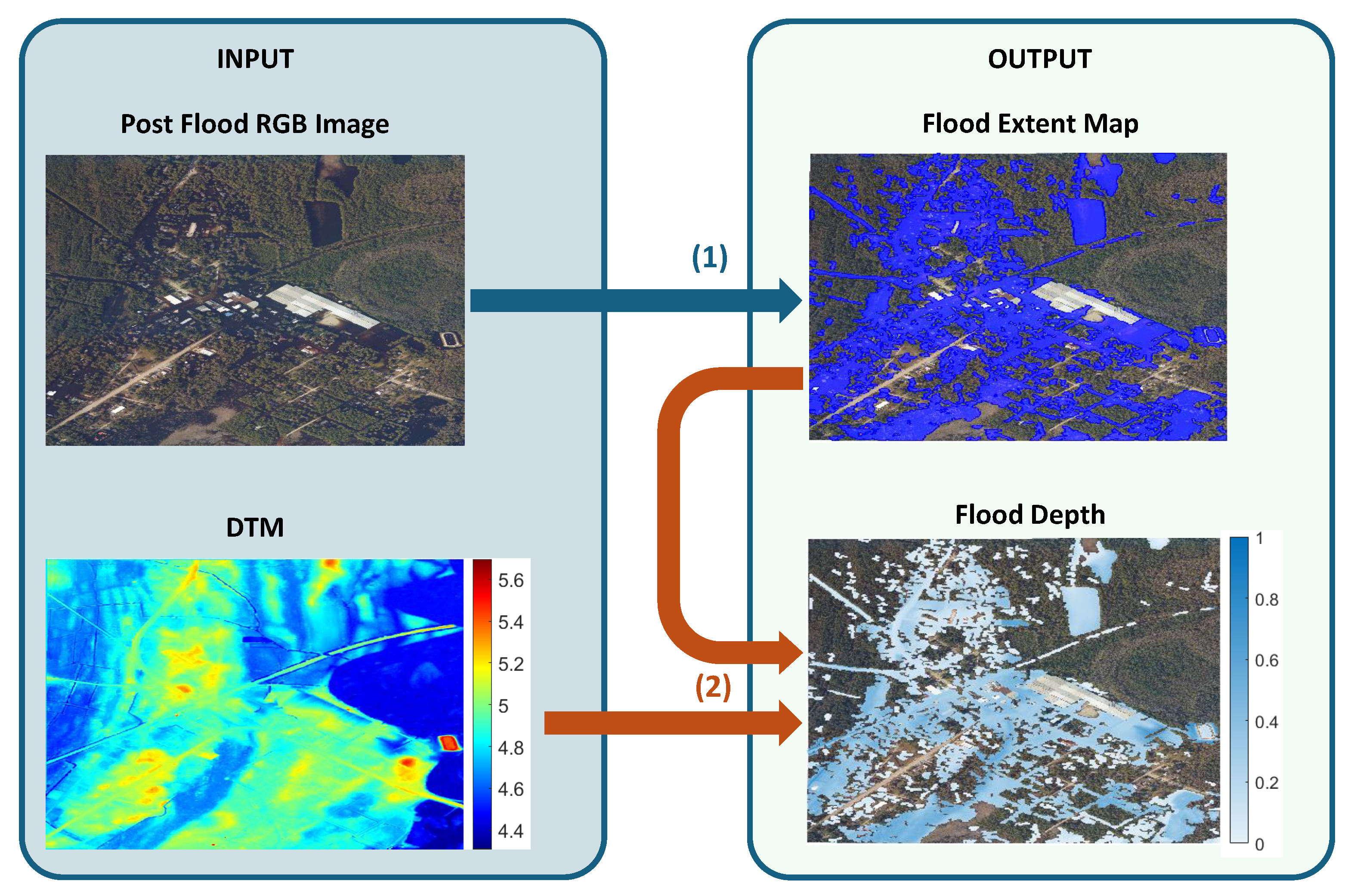
The sole inputs for our unsupervised framework, as illustrated in Figure 1, consist exclusively of post-event aerial imagery and Digital Terrain Models (DTMs):

• Post Flood Aerial Imagery: High resolution optical imagery (approximately 0.25 m spatial resolution) captured shortly after the storm events. Imagery for Hurricane Matthew was acquired between 10–15 October 2016, and for Hurricane Florence on 18 September 2018, originally sourced from the NOAA Storms Archive.
• Digital Terrain Models: High resolution elevation data (approximately 1 m spatial resolution) derived from LiDAR point clouds. These were originally sourced from the North Carolina Emergency Management Spatial Data Portal and the USGS 3D Elevation Program (3DEP). While these products are nominally classified and distributed as bare-earth DTMs, it is important to note that the automated LiDAR point-cloud filtering algorithms used to generate them are rarely perfect. In dense urban or heavily forested catchments, these DTMs frequently retain residual structural artifacts (e.g., imperfectly removed building footprints) and unclassified dense vegetation points.

To demonstrate the rapid response capabilities of the proposed unsupervised approach, the data was ingested and processed using the raw, whole remote sensing images. Unlike previous supervised methodologies [2] applied to this dataset, the images were not subdivided or cropped into standardized tiles (e.g., $256\times 256$ pixel patches). To ensure exact pixel-to-pixel spatial co-registration between the 2D visual data and the 3D topographic data, we utilized the embedded NAD83 coordinate metadata. The 0.25 m optical imagery was rigorously geospatially interpolated to exactly match the 1 m spatial grid of the corresponding DTMs. Consequently, both the unsupervised segmentation and the downstream hydrostatic depth estimation were executed entirely at a 1 m spatial resolution.

Furthermore, the depth estimation relied solely on the extracted flood extent and the raw DTM. No additional hydrologically relevant terrain derivatives, such as slope, surface curvature, or Topographic Wetness Index (TWI), were computed or utilized in this study. By eliminating the requirement for supervised training data, the proposed framework was directly evaluated across the entirety of all 12 urban and peri-urban study sites.

4. Methodology

The proposed framework operates in two distinct phases to achieve scalable, near real time floodwater depth estimation. In the first phase, a binary flood extent map is automatically delineated from high resolution aerial imagery using a modified unsupervised image segmentation algorithm. In the second phase, the extracted two dimensional flood footprints are integrated with the underlying Digital Terrain Model (DTM) to calculate the volumetric flood depth based on the principle of hydrostatic equilibrium. A detailed schematic overview of the proposed framework and its sequential processing stages is presented in Figure 1.

4.1. Unsupervised Flood Extent Delineation

To automatically extract the flood extent without the need for labeled training data or pre disaster imagery, we adopt the foundational architecture of the Unsupervised Flood Segmentation (UFS-HT-REM) framework proposed in [6]. The core principle of this algorithm is to iteratively exclude image regions that confidently belong to the non flood background using a series of parameter free binary masks. While we maintain the overall probability optimization and region growing pipeline of the original framework, we introduce critical modifications to the initialization masks. These adaptations are essential to account for the distinct spatial resolutions, spectral signatures, and atmospheric variables inherent to aerial remote sensing imagery, transitioning the methodology from its original focus on low altitude UAV captures to broad scale aerial observation.

It is important to note that the operational thresholds detailed in this Section are not locally calibrated or optimized against the Inundation2Depth dataset [19]. Rather, they are applied as fixed, a priori heuristics that are either inherited directly from the foundational UFS-HT-REM literature [6] or minimally adapted to account for the transition from low-altitude UAV sensors to wider-scale aerial imagery. By maintaining these as static global parameters across all 12 diverse evaluation sites, the framework preserves its strictly training-free and label-free operational status.

The extraction process consists of the following sequential steps:

• Greenery Exclusion via RGB Vegetation Index

In both urban and rural landscapes, dense vegetation and tree canopies are highly unlikely to be completely submerged. To prevent vegetation from being misclassified as floodwater, we compute the RGB Vegetation Index (RGBVI) [41], which is defined as the normalized difference between the squared green reflectance and the product of blue and red reflectance.

To differentiate vegetation from floodwater across diverse urban and rural topologies, an $RGBVI$ threshold was empirically selected in the context of [6]. The threshold value of $0.0$ accounts for the specific lighting conditions and atmospheric noise present in post hurricane RGB aerial imagery. Pixels with $T{R}_{RGBVI}>0.0$ are classified as definitive background, yielding the first exclusion mask $M_{RGBVI}$.

• LAB Color Space Masking

The imagery is converted into the perceptually uniform CIELAB color space [42], which decouples luminance (L) from chromaticity (A and B). This transformation provides a wide color gamut and enhances robustness against variable illumination conditions [43]. In low altitude acquisitions, such as UAV imagery, floodwater typically exhibits elevated values across all three LAB components relative to the surrounding terrestrial background [6]. Conversely, aerial imagery reveals a distinct spectral behavior: while the A component (red-green axis) remains elevated, both the luminance (L) and the B component (yellow-blue axis) exhibit depressed values. Because the input consists of post-event aerial data, this spectral shift is governed by at-sensor radiance rather than full-column atmospheric effects. The depressed luminance (L) can be attributed to the strong absorption of visible light by water bodies compared to highly reflective urban surfaces. Furthermore, localized path radiance (atmospheric scattering occurring between the ground and the airborne sensor’s altitude) introduces a blue spectral bias that lowers the B component, while the high concentration of optical impurities typical of turbid floodwaters selectively increases reflectance in the red spectrum, maintaining the elevated A component.

To systematically isolate these regions, binary exclusion masks ($M_L$, $M_A$, $M_B$) are computed for each LAB component according to adapted thresholds. Whereas the original framework [6] established classification thresholds by uniformly subtracting the standard deviation from the mean for each LAB component, the aforementioned distinct spectral signatures of airborne derived floodwaters necessitate an adapted approach for components L and B. Consequently, we introduce modified mathematical formulations to define the classification thresholds:

$$\begin{array}{ccc}\hfill {\Delta }_L& =& {\mu }_L+{\sigma }_L,\hfill \end{array}$$

(1)

$$\begin{array}{ccc}\hfill {\Delta }_A& =& {\mu }_A-{\sigma }_A,\hfill \end{array}$$

(2)

$$\begin{array}{ccc}\hfill {\Delta }_B& =& {\mu }_B+{\sigma }_B\hfill \end{array}$$

(3)

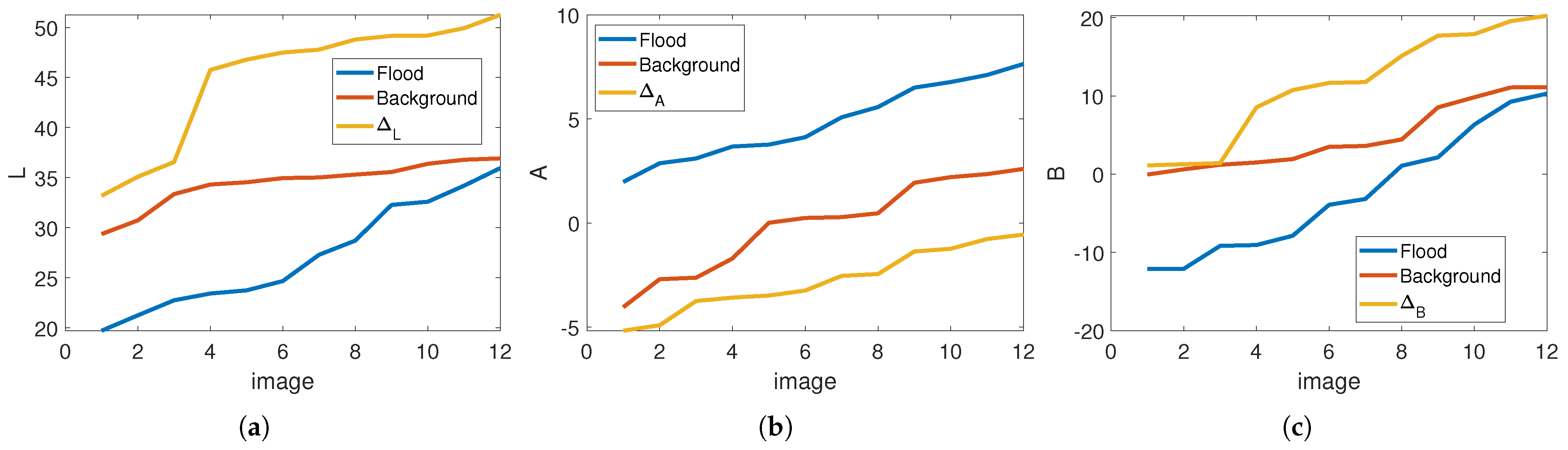
$M_A$ is labeled as non flood, when the component’s pixel value is smaller than ${\Delta }_A$, while $M_L$ and $M_B$ are labeled as non flood when the component’s pixel value is higher than ${\Delta }_L$ and ${\Delta }_B$, respectively. Figure 2 shows the average value of (a) L, (b) A, and (c) B color components computed on flood (blue curve) and background (red curve) pixels for each image of the Inundation2Depth dataset, sorted in ascending order. The yellow curves represent the corresponding thresholds ${\Delta }_L$, ${\Delta }_A$, and ${\Delta }_B$ used to create the three masks. The modified rules were derived heuristically based on the inherent optical physics of water in aerial imagery, specifically its high absorption of light (resulting in lower Luminance, L) and its tendency to reflect ambient sky conditions, rather than through tuning against labeled data. The ground truth masks were absolutely not utilized to design or parameterize these thresholds. Figure 2 utilizes the ground truth masks strictly as a post-hoc statistical analysis to validate the physical soundness of these unsupervised rules and demonstrate why the heuristic separation is effective across the dataset.

These tailored calculations significantly improve algorithmic robustness against the highly heterogeneous spectral signatures characteristic of urban floodwaters, ensuring that only confident background areas are excluded. Furthermore, an edge detection mask ($M_{Edge}$) is derived from the luminance component using the Canny edge detection algorithm [44] on the blurred L component resulting in dilated edges, as to explicitly exclude object boundaries and structural contours from the final flood classification.

• Dominant Color Estimation and Probability Mapping

The union of the five aforementioned masks defines the absolute non flood areas. Consistent classification across all individual masks synergistically increases the confidence of non flood pixel exclusion. Conversely, in regions where a single mask exhibits low discriminative power, the complementary nature of the remaining masks provides functional redundancy, thereby mitigating misclassification. Subsequently, a morphological closing operation is applied to enforce spatial continuity, effectively bridging narrow discontinuities and consolidating proximate, disjointed regions into unified segments.

The remaining unmasked pixels are designated as Potential Flood Areas (PFAs). Under the assumption that pixels further away from confirmed background areas have a higher likelihood of being actual floodwater, a Euclidean distance transform [45] is applied to assign spatial weights to the PFAs. These weighted pixels are then used to estimate the dominant spectral signature of the floodwater. Based on this estimated dominant color, a Gaussian probability map is computed, assigning every pixel in the image a confidence score $[0,1]$ representing its likelihood of being flooded. The complete mathematical formulation governing this spatial weighting and probability estimation process is detailed in [6].

• Final Segmentation via Hysteresis Thresholding

To finalize the binary extent map, hysteresis thresholding is applied to the probability map. Pixels with a probability exceeding a high threshold ($T_H=0.75$) are designated as strong flood seeds. A connectivity based region growing algorithm then expands the flood area from these seeds, absorbing neighboring pixels that exceed a lower threshold ($T_L=0.01$), with both thresholds derived from the ablation study in [6]. This dual threshold approach ensures spatial continuity of the water body while rejecting isolated noise, resulting in a highly accurate, unsupervised flood extent map. Following hysteresis thresholding, the final segmentation undergoes morphological dilation for edge refinement [6].

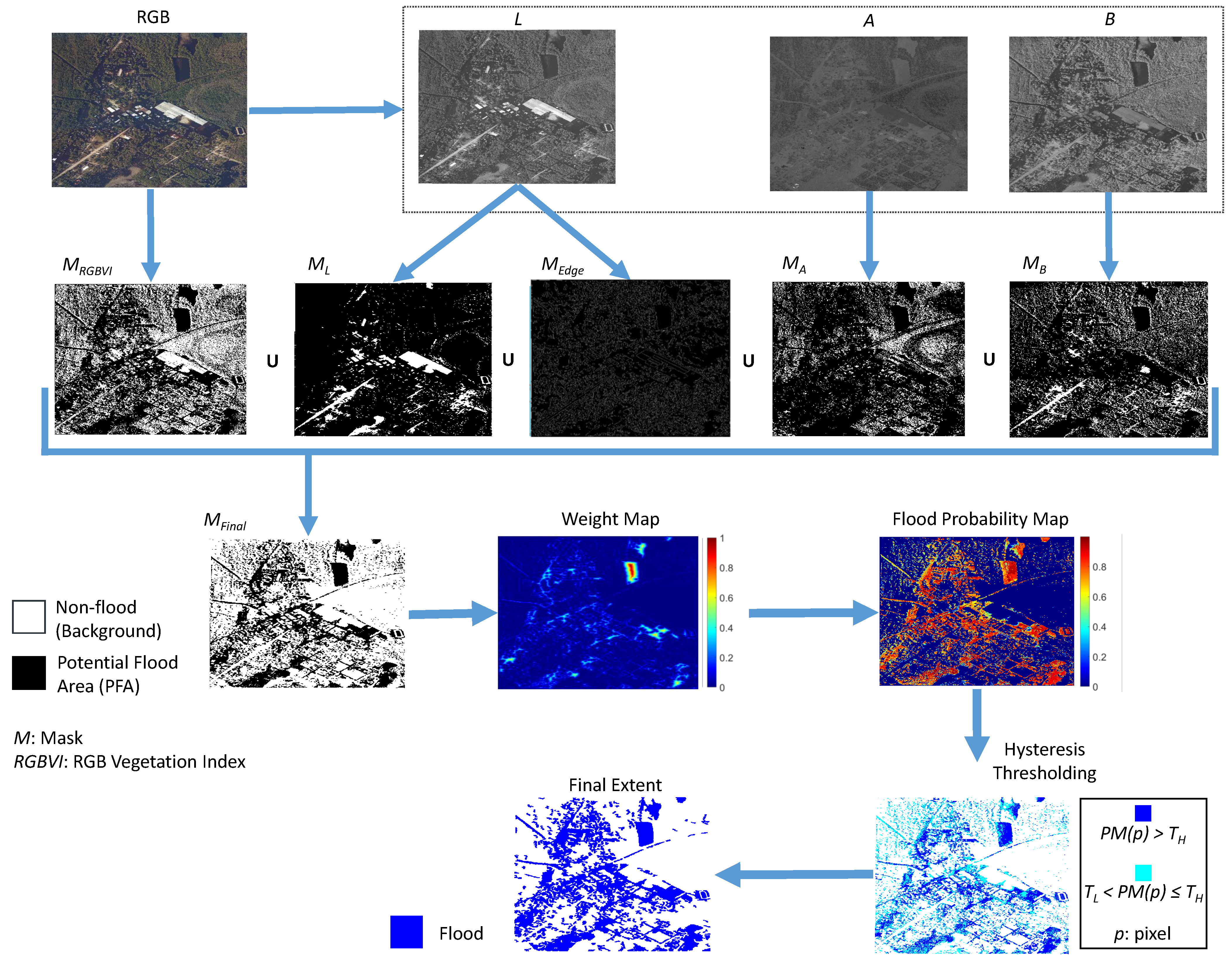
Ultimately, this unsupervised pipeline transitions from broad background exclusion to precise, probability driven region growing, successfully delineating the flood boundaries within complex urban and rural topographies. A schematic overview illustrating the chronological progression of these unsupervised segmentation steps, accompanied by representative visual outputs for each stage, is presented in Figure 3.

4.2. DTM-Based Hydrostatic Flood Depth Estimation

Following the delineation of the two dimensional flood extent map, the volumetric floodwater depth is derived by integrating the spatial flood footprints with the underlying Digital Terrain Model (DTM). This derivation is governed by the physical principle of hydrostatic equilibrium. In the absence of significant momentum, a condition typical of standing or slowly receding post-event floodwaters, water distributes itself to conform to the underlying topography, establishing a relatively smooth, horizontal free surface elevation. Under these steady state conditions, the local flood depth at any given spatial coordinate can be analytically calculated as the vertical differential between the established water surface elevation (WSE) and the localized ground elevation provided by the DTM. The principle is expressed as:

$$H(x,y)=W(x,y)-Z(x,y),$$

(4)

where H, W, and Z are the flood depth, the WSE, and the ground elevation derived from the DTM at coordinates $(x,y)$, respectively, thereby linking the water stage/volume with the flood extent [46].

Because inundation patterns in urban and peri-urban environments are frequently fragmented, yielding multiple spatially disjointed flooded zones, a global WSE cannot be assumed. Therefore, we conceptualize the binary flood extent mask as a set of N discrete, non overlapping connected components, denoted as $\mathcal{C}=\{C_1,C_2,\dots ,C_N\}$, utilizing 8-way pixel connectivity. The selection of 8-way over 4-way connectivity is hydrologically motivated. In high resolution remote sensing imagery, narrow urban flow paths, such as flooded diagonal streets or structural channels, frequently connect only via pixel corners. Utilizing 4-connectivity risks artificially fragmenting a physically continuous water body into multiple isolated sub-regions. Such artificial fragmentation would force the depth module to calculate independent reference water surface elevations for each fragment, creating unrealistic elevation jumps within a single body of water. By employing 8-connectivity, the framework preserves the spatial integrity of the floodwater, ensuring a consistent and continuous elevation estimate across narrow morphological bottlenecks [46].

It is critical to acknowledge that this visual 8-way connectivity serves strictly as an operational proxy for true hydraulic connectivity. In complex urban environments, physical infrastructure, such as road embankments, levees, drainage structures, or partially submerged buildings, can visually connect what are actually hydraulically disjointed water bodies with differing surface elevations. Applying a unified hydrostatic plane across these visually connected but hydraulically distinct zones constitutes a fundamental limitation of the framework. Consequently, the applicability of this method is heavily constrained to relatively static or slowly receding floodwater conditions where dynamic hydraulic gradients have stabilized.

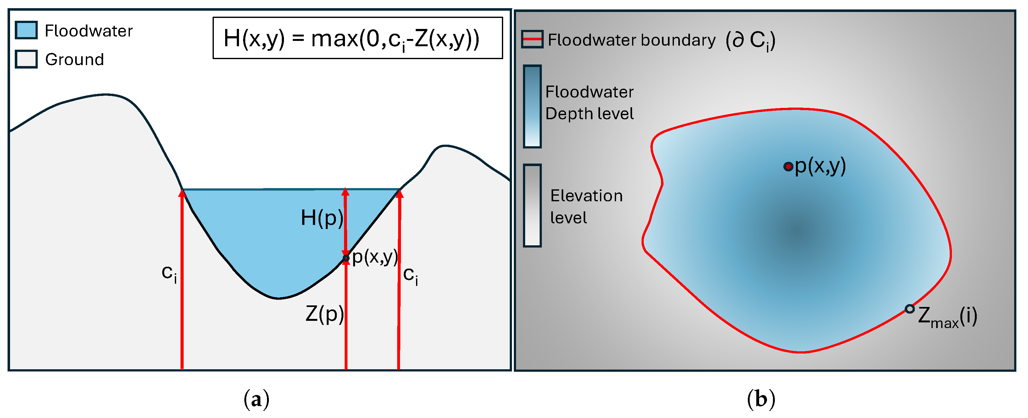
Since the water surface elevation is assumed to be constant within each hydraulically connected flooded region $C_i$, $i\in \{1,\dots ,N\}$, Equation (4) can be reformulated by replacing the spatially varying water surface elevation $W(x,y)$ with a constant reference level $c_i$, $i\in \{1,\dots ,N\}$, representing the estimated water surface elevation for the corresponding flood component $C_i$ (see Figure 4a). Consequently, the local flood depth is expressed as:

$$H(x,y)=max\left(0,c_i-Z(x,y)\right)$$

(5)

The $max(0,·)$ operator enforces the physical constraint that flood depth cannot be negative, ensuring that topographic points located above the estimated water surface are appropriately assigned a zero depth. This generic formulation establishes the mathematical foundation for our localized depth estimators. To operationalize this model, the reference constant $c_i$ is systematically parameterized using specific elevation estimates derived from the discrete flood boundaries, namely the maximum and mean topographic values, as explicitly formalized in Equations (8) and (9).

Algorithmically, this depth estimation protocol is executed independently for each distinct flooded region $C_i$. For any given connected component $C_i$, the physical interaction between the floodwater and the terrain occurs at its spatial boundary. The morphological perimeter of the component $\partial C_i$ contains a set of $|\partial C_i|$ pixels. Under ideal hydrostatic conditions, the local water surface elevation is bounded by the highest topographic point intersecting this boundary. Thus, the local topography at the perimeter dictates the potential maximum WSE for that specific flooded depression. The absolute maximum terrain elevation along the perimeter is defined as:

$$Z_{max}\left(i\right)=\underset{(x,y)\in \partial C_i}{max}Z(x,y).$$

(6)

However, relying exclusively on $Z_{max}\left(i\right)$ renders the estimation highly susceptible to localized DTM anomalies, such as unclassified canopy remnants, minor structural artifacts, or boundary misclassifications. To mitigate these outlier effects and establish a more robust surface estimate, the mean topographical elevation along the entire perimeter is concurrently calculated:

$$Z_{mean}\left(i\right)={\displaystyle \frac{1}{|\partial C_i|}}\sum _{(x,y)\in \partial C_i}Z(x,y)$$

(7)

To estimate the local flood depth for each pixel $(x,y)\in C_i$, we introduce a weighted formulation based on two independent local depth estimates. The first estimate is derived from the maximum boundary elevation, while the second is derived from the mean boundary elevation. These quantities are defined as

$$H_{max}(x,y)=\left\{\begin{array}{cc}max\left(0,Z_{max}\left(i\right)-Z(x,y)\right),\hfill & (x,y)\in C,\hfill \\ 0,\hfill & (x,y)\notin C,\hfill \end{array}\right.$$

(8)

$$H_{\mathrm{mean}}(x,y)=\left\{\begin{array}{cc}max\left(0,Z_{mean}\left(i\right)-Z(x,y)\right),\hfill & (x,y)\in C,\hfill \\ 0,\hfill & (x,y)\notin C.\hfill \end{array}\right.$$

(9)

The flood depth is then computed as a weighted linear combination of the two estimates:

$$\widehat{H}(x,y)=(1-w)·H_{max}(x,y)+w·H_{\mathrm{mean}}(x,y),$$

(10)

where $w\in [0,1]$ serves as a weighting coefficient that regulates the influence of the mean elevation against the absolute physical upper bound. In our experiments, we set $w={\displaystyle \frac{1}{2}}$, such that the two depth components contribute equally to the flood depth estimate $\widehat{H}$. Consequently, $\widehat{H}(x,y)$ corresponds to the arithmetic average of $H_{max}(x,y)$ and $H_{\mathrm{mean}}(x,y)$, ensuring that neither the maximum- nor the mean-boundary-based estimate dominates the solution. This choice reflects a neutral weighting scheme that balances the physically conservative nature of the maximum elevation criterion with the more representative characterization provided by the mean boundary elevation. The application of the $max(·,·)$ operator to each individual depth estimate is mathematically critical to ensure that internal topographic features (e.g., elevated terrain or structural islands enclosed within the flood boundary) correctly yield zero local flood depth. This preserves the physical constraints imposed by the terrain and prevents the generation of non-physical negative depth values.

Finally, to eliminate sharp local discontinuities and yield a physically realistic, smooth final depth profile H, the aggregated depth map $\widehat{H}$ undergoes spatial smoothing via convolution with a $5\times 5$ Gaussian kernel $G_{\sigma }$ with $\sigma =1$:

$$H(x,y)=\widehat{H}(x,y)\ast G_{\sigma }(x,y),$$

(11)

where ∗ denotes the 2D convolution operator.

Figure 4 provides a conceptual overview of the proposed DTM-based flood depth estimation framework. The cross-sectional view in Figure 4a illustrates the generic depth formulation, where the flood depth at any point $p(x,y)$ is defined as the positive difference between the reference water surface elevation $c_i$ and the corresponding terrain elevation $Z(x,y)$. The plan-view representation in Figure 4b demonstrates the proposed spatial implementation of this principle, where the floodwater boundary (red) defines the flooded region used to estimate the reference water level, and the blue and gray color gradients depict the resulting flood depth distribution and the underlying terrain elevation, respectively. Together, these schematics illustrate the physical basis of the proposed method and its application to DTM-based flood depth estimation.

Figure 5 visually illustrates the sequential outcomes of this depth estimation framework. Specifically, Figure 5a and Figure 5b display the independent depth profiles generated using the absolute maximum ($H_{max}$) and mean ($H_{\mathrm{mean}}$) perimeter elevations, respectively. The arithmetic average of these two bounds, representing the balanced but weighted depth ($\widehat{H}$), is shown in Figure 5c. Finally, the post-processed depth map following Gaussian convolution (H) is presented in Figure 5d, demonstrating the successful mitigation of sharp local discontinuities to yield a continuous, physically plausible volumetric floodwater profile.

5. Experimental Setup

5.1. Implementation Details and Computational Efficiency

The proposed methodology was implemented using MATLAB 2023b. All experimental simulations and evaluations were executed on a standard laptop equipped with an Intel Core i7 CPU processor operating at 2.3 GHz and 40 GB of RAM.

A significant architectural advantage of the proposed unsupervised algorithm is its computational efficiency and linear complexity, with both the segmentation and depth estimation modules operating at $O\left(n\right)$ linear complexity relative to the total number of pixels n. While the method achieves a typical inference time of approximately 3 s for a standard $2000\times 1400$ pixel image, it scales exceptionally well to larger, more complex geographic extents. For the largest study site in our dataset (Lumberton, $5848\times 7244$ pixels), the end-to-end framework completes in just 42.11 s. Across all 12 diverse study sites, processing times ranged from 0.21 s to 42.11 s for images with 0.27 to 42.36 megapixels respectively, with an average time of 8.83 s per catchment. Statistical analysis of these empirical benchmarks confirms a highly linear scaling behavior (Pearson’s $r=0.96$), processing at an average rate of approximately 0.94 s per megapixel. This performance is achieved using purely CPU-based processing, successfully bypassing the necessity for the power-intensive GPU cores required by heavy DL models.

Because of its low time computational cost and minimal hardware resource requirements, the proposed framework is highly suitable for rapid, on-site deployment on standard laptops, enabling immediate execution by emergency response personnel during active disaster scenarios. To ensure reproducibility and facilitate future research, the source code implementing the proposed method, alongside detailed experimental results, is publicly available at the following repository: https://sites.google.com/site/costaspanagiotakis/research/flood-detection (accessed on 3 August 2026).

5.2. Evaluation Metrics

To assess the dual outputs of our framework, distinct evaluation metrics are employed for the 2D flood extent segmentation and the 3D volumetric depth estimation. For the binary flood extent map, the spatial agreement between the predicted flooded areas and the ground truth annotations is quantified using the F₁-score metric, defined as:

$$F1={\displaystyle \frac{2·TP}{2·TP+FP+FN}},$$

(12)

where $TP$, $FP$, and $FN$ represent the number of true positive, false positive, and false negative pixels, respectively.

For the flood depth estimation, the accuracy of the predicted water levels is evaluated using standard regression metrics, specifically the Root Mean Square Error (RMSE) and the Mean Absolute Error (MAE). Let $C_{gt}$ denote the set of spatial coordinates corresponding to the valid flooded pixels within the ground truth mask, such that for all $(x,y)\in C_{gt}$, the ground truth depth is strictly positive ($H_{gt}(x,y)>0$). The total number of these valid pixels is represented by $|C_{gt}|$. To quantitatively evaluate the predictive accuracy of a flood depth estimation model, the Root Mean Square Error (RMSE) and Mean Absolute Error (MAE) are calculated over these localized flooded regions. Measured in meters (m), these absolute evaluation metrics are formally defined as follows:

$$\mathrm{RMSE}=\sqrt{{\displaystyle \frac{1}{|C_{gt}|}}{\sum }_{(x,y)\in C_{gt}}{\left(H(x,y)-H_{gt}(x,y)\right)}^2}$$

(13)

$$\mathrm{MAE}={\displaystyle \frac{1}{|C_{gt}|}}\sum _{(x,y)\in C_{gt}}\left|H(x,y)-H_{gt}(x,y)\right|,$$

(14)

where $H(x,y)$ is the estimated flood depth at pixel $(x,y)$, and $H_{gt}(x,y)$ is the corresponding true depth derived from the ground truth data.

Furthermore, to provide a scale-independent assessment of relative depth accuracy across catchments with differing flood magnitudes, we report the maximum-normalized RMSE (nRMSE) and maximum-normalized MAE (nMAE). Normalizing by the maximum ground truth depth ensures mathematical stability and prevents the artificial error inflation that typically plagues traditional relative metrics at shallow inundation boundaries. These are defined as:

$$\mathrm{nRMSE}={\displaystyle \frac{\mathrm{RMSE}}{max\left(H_{gt}\right)}},\mathrm{and}\mathrm{nMAE}={\displaystyle \frac{\mathrm{MAE}}{max\left(H_{gt}\right)}},$$

(15)

where $max\left(H_{gt}\right)$ represents the maximum recorded ground truth depth within the specific catchment. Maximum depth was selected for normalization rather than mean depth because urban flood extents are often dominated by vast areas of shallow, peripheral water. Normalizing by a low mean depth would artificially inflate the relative error metric. Furthermore, because the minimum depth of a flooded pixel is inherently bounded at zero, normalizing by the maximum depth is mathematically equivalent to normalizing by the total depth range.

As detailed in Section 3, direct, spatially continuous flood depth observations were unavailable across the multiple study sites. Given that the ground truth generation process inherently relies on the DTM and assumes hydrostatic conditions, the reference depth maps are not entirely independent of the underlying terrain data. Consequently, the RMSE and MAE metrics reported in this study should not be interpreted as deviations from a perfect physical ground truth. Rather, they quantify the capability of our strictly unsupervised approach to approximate a heavily calibrated, semi-manual reference model that benefited from external HWMs and hydrodynamic validation.

6. Experimental Results and Discussion

In this section, we present a comprehensive experimental evaluation of the proposed unsupervised framework. To rigorously assess the dual outputs of our pipeline, we provide both quantitative metrics and qualitative visual analyses for its two core stages: (1) flood region segmentation, and (2) flood depth estimation. Furthermore, a parameter sensitivity analysis is conducted to systematically evaluate the a priori thresholds utilized in the segmentation stage, and the weighted contributions of the maximum and mean boundary elevation estimates, as defined in Equations (8) and (9) respectively, to the final predictive accuracy. Also, the topological and morphological drivers with respect to the error of our flood depth estimation module are explored. Finally, to contextualize the algorithmic efficiency and physical validity of the proposed framework, we conclude with a comparative evaluation against baselines.

6.1. Flood Region Segmentation Performance

The evaluation of the flood extent delineation stage, summarized under the semantic segmentation metrics in

Table 3. Comprehensive quantitative evaluation of the proposed unsupervised framework across the 12 study sites, sorted in ascending order of nRMSE. The table presents performance metrics for both the 2D flood region segmentation stage (Intersection over Union (IoU), F₁-score, Precision (Pr), Recall (Rec), and Accuracy (Acc)), and the flood depth estimation stage (Root Mean Square Error (RMSE) in meters, Mean Absolute Error (MAE) in meters, maximum-normalized RMSE (nRMSE), and maximum-normalized MAE (nMAE)). Upward arrows (↑) indicate that higher values correspond to better performance, while downward arrows (↓) signify that lower error values are preferable.

Site	Flood Region Segmentation					Flood Depth Estimation
	IoU ↑	F1 ↑	Pr ↑	Rec ↑	Acc ↑	RMSE ↓	MAE ↓	nRMSE ↓	nMAE ↓
Princeville	0.7431	0.8526	0.8026	0.9093	0.9122	0.9664	0.6860	0.1376	0.0977
Goldsboro1	0.6617	0.7964	0.8658	0.7373	0.8790	1.1085	0.7996	0.1553	0.1120
HancheysStore	0.9288	0.9631	0.9633	0.9629	0.9551	0.9326	0.8084	0.1672	0.1449
Chinquaqin	0.8480	0.9177	0.9726	0.8687	0.9007	0.4912	0.3976	0.1698	0.1374
Lumberton	0.6920	0.8180	0.8197	0.8162	0.9213	1.1811	0.8462	0.1700	0.1218
Nichols	0.6686	0.8014	0.7086	0.9221	0.8774	0.1649	0.1313	0.1715	0.1366
Greenville1	0.6604	0.7955	0.7475	0.8500	0.9302	0.6260	0.4451	0.1807	0.1285
Kinston1	0.4968	0.6638	0.9136	0.5213	0.8788	1.5823	1.2420	0.1811	0.1421
Kinston2	0.5810	0.7350	0.8762	0.6330	0.8772	0.8942	0.6642	0.1882	0.1398
Greenville2	0.7719	0.8713	0.8398	0.9052	0.9256	1.1572	0.8713	0.1892	0.1424
Wallace	0.7651	0.8669	0.9802	0.7771	0.8399	0.9119	0.6916	0.2241	0.1700
Goldsboro2	0.4595	0.6296	0.8694	0.4935	0.7257	1.6861	1.2982	0.2514	0.1936

, demonstrates that the proposed unsupervised method achieves robust and reliable segmentation performance across regional urban and peri-urban environments. Because our depth estimation stage relies entirely on hydrostatic equilibrium constraints sampled from extracted boundaries, establishing a high-fidelity flood extent mask is vital. The experimental results show that our framework successfully captures intricate flood distributions without requiring any manual supervision or pre-training.

When categorized by overall segmentation quality, the highest F₁-scores were obtained in catchments HancheysStore (F₁ = 0.9631, IoU = 0.9288, Accuracy = 0.9551), and Chinquaqin (F₁ = 0.9177, IoU = 0.8480, Accuracy = 0.9007). These outstanding metrics indicate that the unsupervised boundary delineation module handles continuous, wide-area water layers excellently, producing extremely sharp region outlines that minimize both false positive and false negative pixel assignments. Moreover, the model maintains high structural stability even in more fragmented peri-urban landscapes. Sites like Greenville2 and Princeville exhibit stable segmentation capabilities with comparable F₁-scores of 0.8713 and 0.8526, respectively, combined with strong pixel-level accuracy metrics exceeding 90%.

Furthermore, an analysis of the relationship between Precision and Recall reveals the conservative nature of our unsupervised delineation module. The consistently high Precision scores across the dataset, ranging from 71% to 98%, demonstrate that the method is highly resilient against false alarms (False Positives) caused by non-flooded urban features with dark spectral responses. Conversely, the lowest segmentation performance was recorded at the Kinston1 and Goldsboro2 catchments, yielding F₁-scores of 0.6638 and 0.6296, respectively. High Precision (91% and 87%, respectively) is maintained at the expense of Recall (52% and 49%, respectively), reflecting omission errors (False Negatives). This localized degradation is primarily driven by extreme visual fragmentation and structural occlusions inherent to the site’s layout, alongside localized shadow and reflectance issues.

Overall, despite the slight performance variations the framework maintains a pixel accuracy above 87% across 10 of the 12 study catchments. This consistent performance underscores the regional generalizability and effectiveness of our label-free unsupervised approach, validating its suitability as a robust, automated mask generation module for downstream hydrological calculations in urban and peri-urban environments.

6.2. Flood Depth Estimation Performance

From the flood depth estimation metrics (columns 7–10 of Table 3), the maximum-normalized RMSE (nRMSE) serves as our primary performance metric, as it provides a scale-independent assessment of relative depth accuracy across catchments with differing flood magnitudes. As demonstrated in Table 3, our unsupervised framework achieved strong relative precision (nRMSE < 0.17) in sites such as Princeville (nRMSE = 0.1376), Goldsboro1 (nRMSE = 0.1553), HancheysStore (nRMSE = 0.1672), and Chinquaqin (nRMSE = 0.1698). In these well-defined flooding events, minor spatial misalignments along the delineated edge borders translate into negligible relative depth errors, validating the robustness of our hydrostatic equilibrium assumptions across wide-area topographies when floodwater is standing or slowly receding.

Moving beyond the top performers, catchments such as Lumberton, Nichols, Greenville1, and Kinston1 demonstrate intermediate, yet highly stable, depth estimation accuracy, yielding an average nRMSE of 0.1758. In these mid-performing scenarios, the recorded average MAE of the proposed methods can be considered adequate for regional-scale emergency mapping and broad resource allocation.

Analyzing these results in the context of the spatial classification metrics highlights the non-linear relationship between 2D pixel accuracy and 3D hydrostatic fidelity. Because the terrain-to-depth mapping phase extracts its vertical references strictly from the delineated margins, the severity of the 3D depth error is ultimately dictated by the specific topographic gradients present at those boundary pixels, rather than global segmentation metrics alone. For instance, despite achieving above-average global segmentation scores and high Recall, catchments like Greenville2 (F₁ = 0.8713, Recall = 0.9052) and Wallace (F₁ = 0.8669, Recall = 0.7771) exhibit elevated relative depth errors, with nRMSE values of 0.1892 and 0.2241, respectively. This quantitative divergence demonstrates that even when 2D boundaries are well-captured, mathematically negligible boundary variations can coincidentally align with steep elevation gradients or uncorrected micro-topographic artifacts in the underlying DTM, thereby sampling unrepresentative elevations and gently warping the localized hydrostatic plane.

Conversely, the most pronounced degradations occur when severe 2D omission errors shift the sampling margin significantly inward, forcing the algorithm to rely on highly unrepresentative baselines. In Kinston1, a significant drop in horizontal segmentation quality (F₁ = 0.6638, Recall = 0.5213) surprisingly yields a relatively controlled depth error (nRMSE = 0.1811), indicating that the omitted boundaries were located on relatively flat, forgiving topological gradients. However, in Goldsboro2, similar segmentation failures (F₁ = 0.6296, Recall = 0.4935) lead to severe absolute depth discrepancies (RMSE = 1.6861 m, MAE = 1.2982 m, nRMSE = 0.2514). Missing over half of the true flood boundary forces the algorithm to sample elevations from interior topographic pixels, propagating artificially skewed baselines throughout the hydrostatic-based depth estimation module. Nevertheless, bounding the maximum relative error at roughly 0.25 across these most computationally and optically challenging scenarios highlights the practical resilience of this label- and training-free deployment strategy.

When interpreting these quantitative error metrics, the temporal mismatch between the imaged stage and the reference depths must be explicitly accounted for. Because the ground truth depth models correspond to the flood peak, while our framework delineates the recession-stage water boundaries captured in the post-event imagery, the extracted water surface elevations are inherently lower than the peak reference. Consequently, a distinct portion of the reported RMSE and MAE does not represent algorithmic modeling error, but rather physically quantifies the temporal drawdown of the water level that occurred between the storm’s peak and the aerial image acquisition. Furthermore, because the dataset’s reference depth maps are not derived from spatially continuous physical sensors, but rather generated using empirical HWMs and HEC-RAS hydrodynamic simulations, these error metrics should not be interpreted as deviations from a perfect physical ground truth.

Notably, while Blay et al. [18] provide the only competing method on this dataset, a direct quantitative comparison of absolute errors is structurally invalid due to three fundamental methodological divergences:

• Their framework relies on a supervised learning paradigm, dividing the dataset to train their models on thousands of localized patches, giving the network prior spatial knowledge of the regional topography. In contrast, our approach is entirely unsupervised and training-free, operating without prior geographic exposure.
• To establish their reference data, the authors applied systematic manual corrections to their initial flood extent masks to mitigate omission and commission errors. Our pipeline derives horizontal boundaries completely automatically.
• Their reported evaluation metrics correspond to just one unseen catchment (in Scenario 2), and their site-level depth errors, calculated exclusively at sparse High Water Mark (HWM) locations (often relying on just 2–4 points per catchment), serve solely to validate the dataset’s generated ground truth.

Because their work already establishes that this dense ground truth reliably reflects physical HWMs, our study utilizes it to compute rigorous, pixel-wise performance metrics continuously across the entire 2D flood extent. Consequently, while both studies provide valuable insights, a direct comparison is inappropriate.

6.3. Qualitative Analysis and Depth Error Mapping

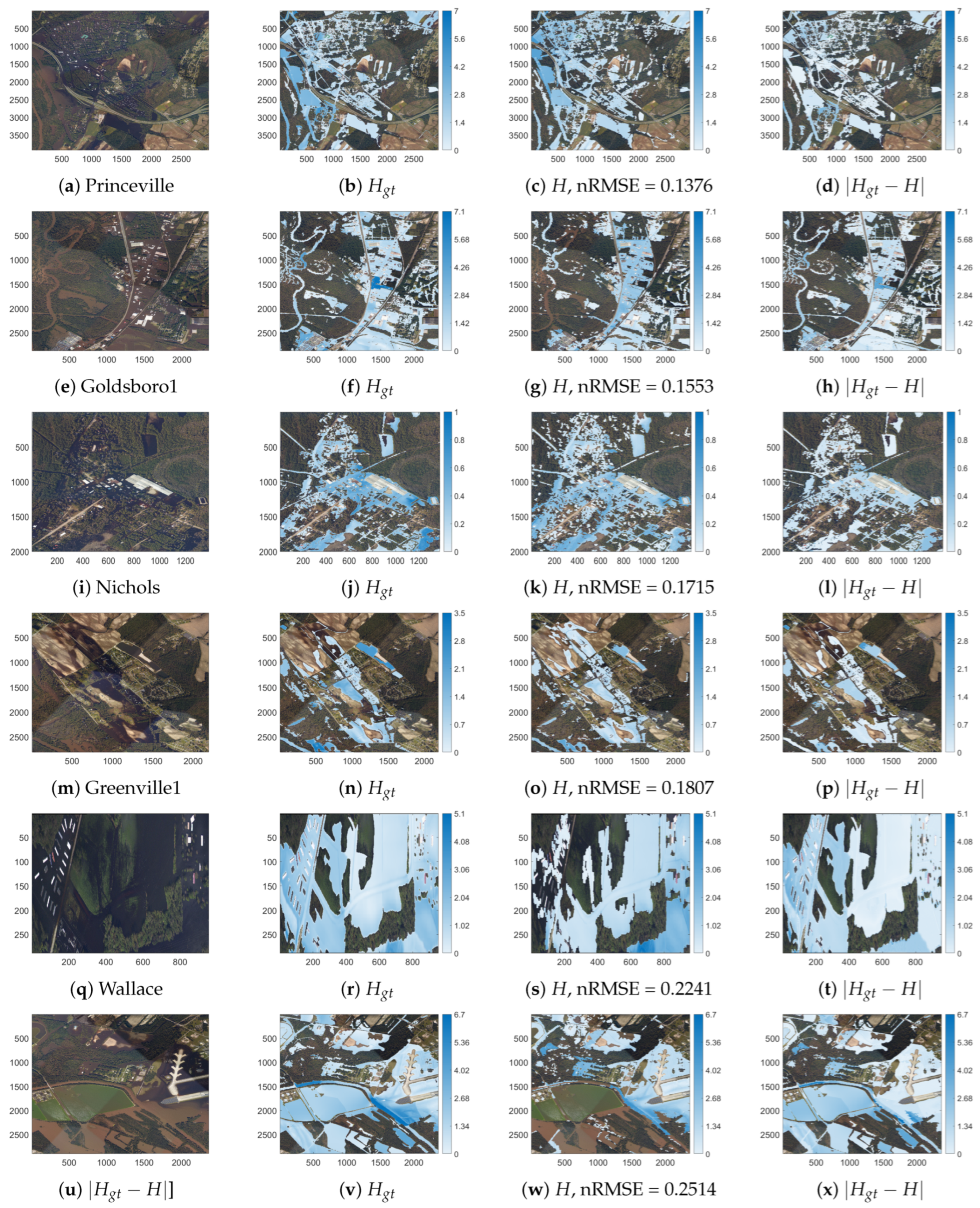
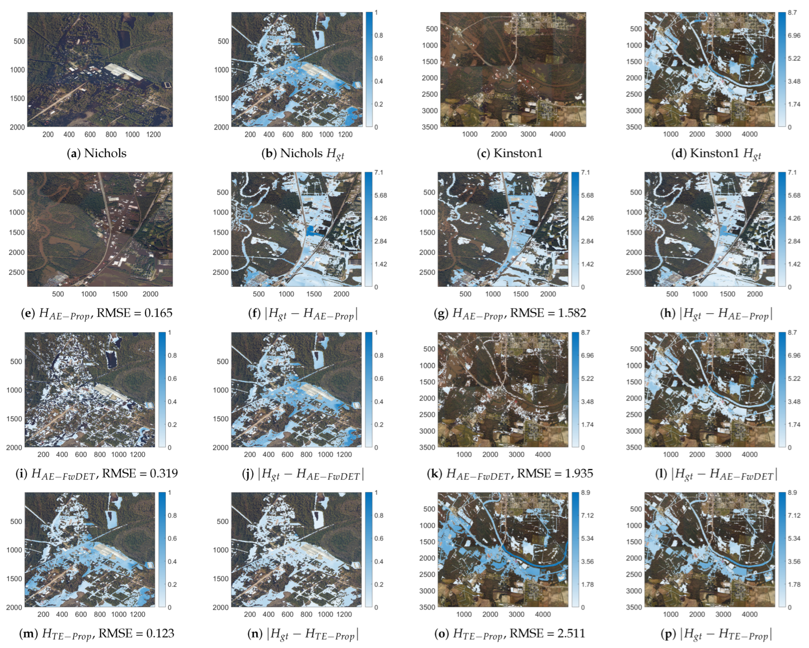
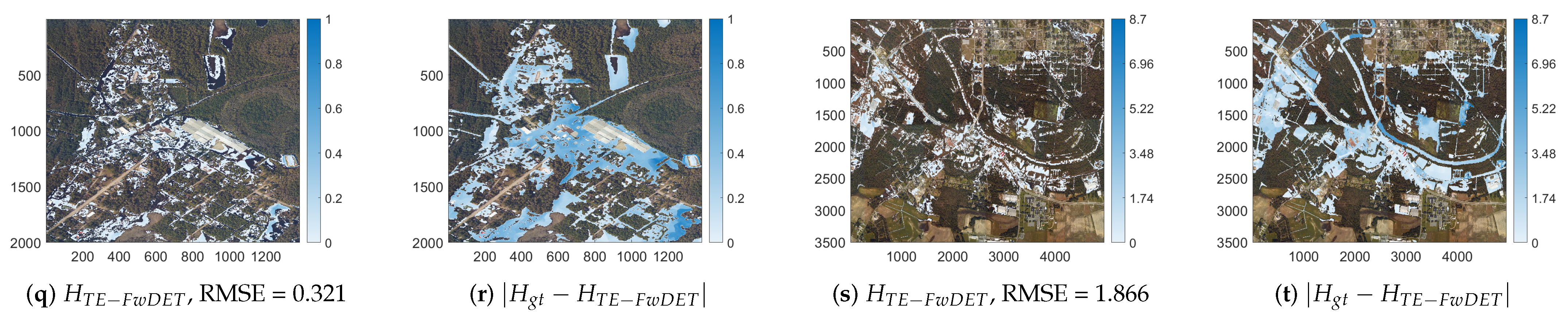
To evaluate the spatial robustness of the proposed unsupervised depth estimation framework in the study dataset, Figure 6 illustrates a side-by-side qualitative comparison across six representative catchments. The study sites are arranged hierarchically by relative performance based on their maximum-normalized RMSE. The first two rows present the highest-performing cases (Princeville and Goldsboro1), followed by the mid-performing catchments in the third and fourth rows (Nichols and Greenville1), and concluding with the most challenging, worst-performing scenarios (Wallace, Goldsboro2) in the final two rows.

The first two rows demonstrate that in our best-performing cases, the unsupervised depth maps closely mirror the structural topology of the ground truth. Because Princeville and Goldsboro1 generally feature widespread flood coverage, the boundary extraction module successfully isolates clean land-water interfaces. This allows the localized hydrostatic equilibrium sampler to anchor its vertical height references accurately, minimizing relative depth fluctuations across the vast majority of the water surface.

Looking specifically at Princeville, the absolute error map ($|H_{gt}-H|$) for this region, depicted in Figure 6d, confirms a near-perfect baseline extraction, and is primarily characterized by a highly uniform, low-magnitude error profile dominated by the pale cyan and white spectrum, which corresponds to near-zero vertical discrepancies. In contrast, while Goldsboro1 maintains highly accurate overall depth estimation, it introduces specific localized artifacts. As evident when comparing Figure 6f,g, the segmentation stage exhibits omission errors, most notably in the forested bottom-left quadrant. Furthermore, the absolute error map for Goldsboro1 reveals a concentrated pocket of higher discrepancy, visible as the dark blue patch in the central-right corridor in Figure 6h. This contrast indicates that even within highly accurate global estimations, isolated DTM anomalies, undetected structural barriers, or localized boundary occlusions can still perturb the hydrostatic plane on a microscale.

Moving to the mid-performing catchments in the third and fourth rows (Nichols and Greenville1), the visual comparisons illustrate the framework’s response to complex landscapes and challenging optical conditions. In these scenarios, the 2D segmentation stage experiences omission errors and over segmentation compared to the top performers. Although both feature an F₁-score around 80%, the relatively stable nRMSE scores (0.1715 and 0.1807, respectively) demonstrate that the correctly extracted boundaries still sample representative topographic elevations, preventing the hydrostatic plane from skewing drastically.

Examining Nichols (Figure 6i), the environment features a highly fragmented flood extent disrupted by dense vegetation and infrastructure. While the predicted depth map (Figure 6k) noticeably oversegments compared to the ground truth (Figure 6j), the absolute error map in Figure 6l remains remarkably uniform in the near-zero (white to pale cyan) range. Conversely, Greenville1 (Figure 6m) suffers from optical ambiguities, such as darkly shadowed terrain and low spectral contrast in turbid waters, which cause substantial boundary omissions, particularly in the upper and lower-left quadrants (Figure 6o). Because these omitted boundaries force the algorithm to sample elevations further inward, the absolute error map (Figure 6p) displays more concentrated, localized pockets of higher vertical discrepancy (visible as moderate blue patches). This perfectly illustrates how shifting the detection boundary over varying topographic gradients directly warps the localized depth estimation, even when the overall regional metric remains stable.

The final rows represent the highly complex catchments of Wallace and Goldsboro2, which exhibit the most pronounced vertical discrepancies. Visually, Goldsboro2 suffers from a heavily degraded segmentation (F₁ = 0.6296), as can be observed by comparing Figure 6v,w, where large flooded areas failed to be delineated. A visual inspection reveals a flooded airport facility and adjacent basins where dark, turbid water blends seamlessly with dense greenery and prominent cloud shadows. This lack of spectral contrast leads the unsupervised method to miss massive, contiguous subregions of water. Because our terrain-to-depth mapping phase extracts its vertical references directly from these water margins, this severe omission error forces the hydrostatic-based depth estimation module to sample incorrect interior elevations, propagating severe errors throughout the pipeline (nRMSE = 0.2514).

Conversely, Wallace achieves a higher segmentation score (F₁ = 0.8669), yet still struggles with depth estimation (nRMSE = 0.2241). The raw imagery depicts a densely wooded residential zone heavily obscured by a massive optical shadow (Figure 6q). The algorithm segments around the scattered houses and canopies, but this creates a highly porous, fragmented mask. Consequently, the boundary pixels could physically align with residual LiDAR classification artifacts (e.g., imperfectly filtered rooftops and dense root systems remaining in the DTM) rather than the true bare-earth waterline (Figure 6s). Sampling from these artificial DTM elevations induces the extreme localized depth fluctuations seen in Figure 6t. However, these perceived algorithmic failures must be contextualized by the inherent temporal offset. Because the ground truth models the peak inundation stage, while the proposed framework maps the receded, contemporaneous waterline, a significant portion of this numerical error reflects the physical water drawdown rather than pure geometric failure. Furthermore, this highlights a fundamental limitation: the accuracy of any terrain-to-depth mapping is bounded by the quality of the underlying DTM. In environments like Wallace, when uncorrected micro-topographic artifacts, structural footprints or vegetation biases coincide with the highly fragmented, recession-stage flood margins, they introduce erroneous vertical references into the hydrostatic-based depth estimation module. When compounded with the temporal misalignment of the peak ground truth, this drives severe depth estimation errors despite a highly accurate 2D segmentation.

6.4. Parameter Sensitivity Study

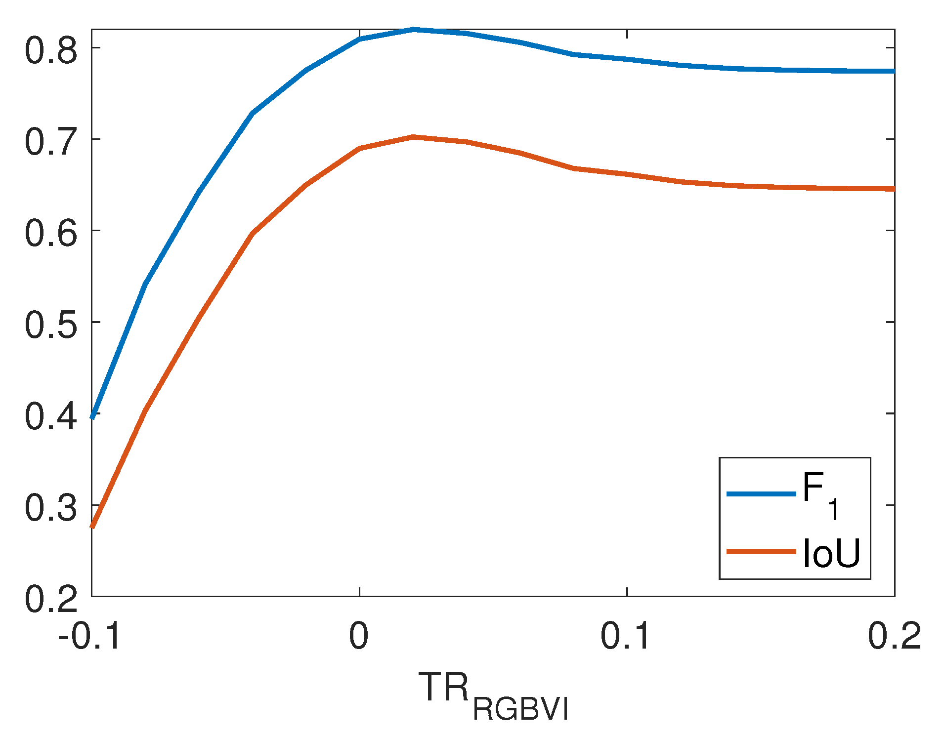
To verify the robustness of the framework’s static parameters, used in the segmentation stage, against varying optical conditions, such as varying water turbidity, structural shadows, and inconsistent lighting, a comprehensive parameter sensitivity analysis was conducted across the dataset. We first evaluate the RGBVI threshold, analyzing the global segmentation performance ($F_1$-score and IoU) across a threshold range from −0.1 to 0.2.

As illustrated in the sensitivity curves in Figure 7, the segmentation module’s accuracy experiences a sharp decline for negative threshold values and a more gradual degradation as the threshold increases beyond the optimal range. Crucially, while the absolute mathematical peak is achieved at a marginally positive value (approximately 0.02), the globally applied a priori heuristic of $T{R}_{RGBVI}=0.0$ yields a near-optimal performance that is virtually indistinguishable from the absolute maximum. This empirical behavior confirms that a static, uncalibrated threshold of 0 provides a highly resilient global optimum across the diverse spatial and optical conditions of the Inundation2Depth dataset. Consequently, this validates the framework’s strictly training-free operational status, demonstrating that site-specific calibration of the vegetation index is unnecessary for extracting robust flood boundaries.

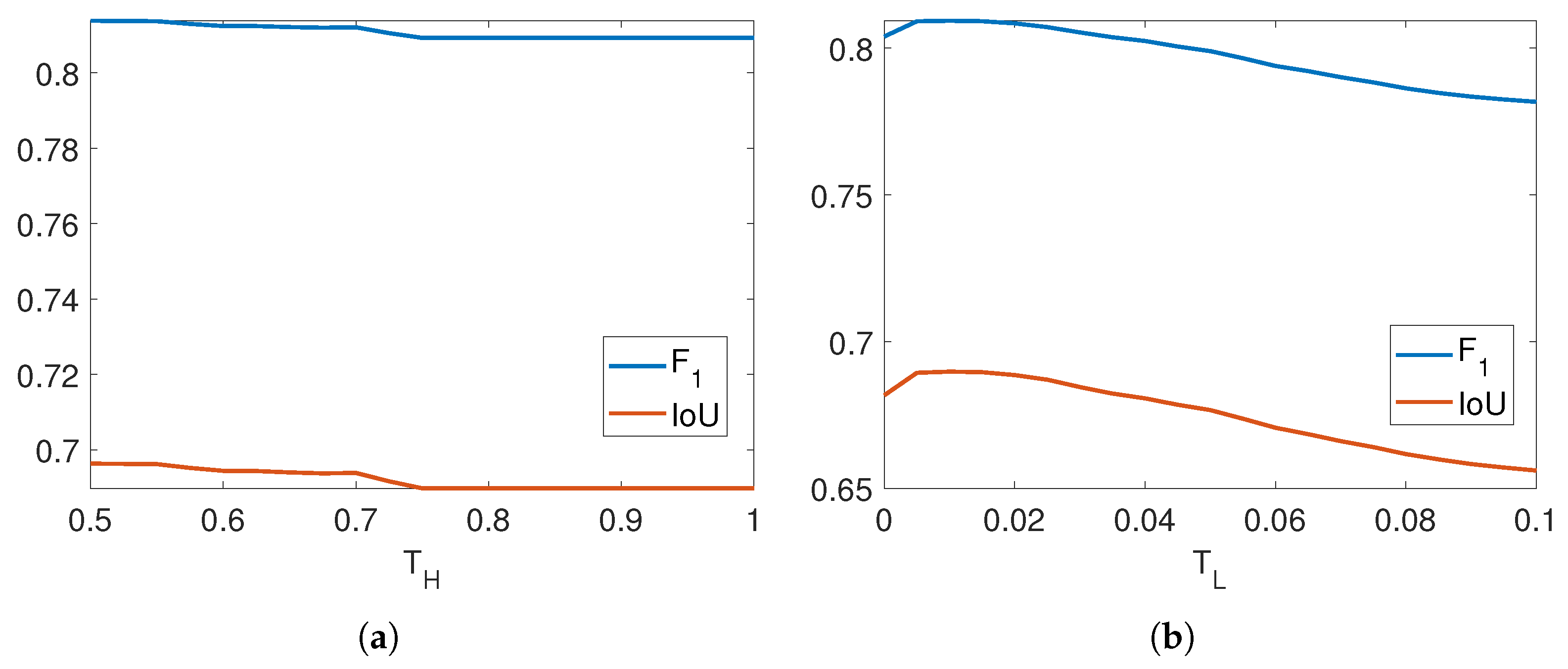
Following the validation of the greenery exclusion heuristic, a similar sensitivity analysis was conducted for the hysteresis segmentation parameters ($T_H$ and $T_L$), which respectively govern the high-confidence seed generation and the subsequent region growing phases of the flood extent delineation module. As depicted in Figure 8a, the framework exhibits extreme stability with respect to the high threshold $T_H$ (when $T_L=0.01$). Across the entire evaluated range from 0.5 to 1.0, both the global $F_1$-score and IoU remain virtually flat, indicating that the initial identification of unoccluded flood pixels is highly robust and entirely insensitive to strict local calibration.

Similarly, the evaluation of the low threshold $T_L$ (when $T_H=0.75$) shown in Figure 8b, reveals a broad plateau of near-optimal performance. While a slight mathematical peak occurs at approximately $T_L=0.01$, the evaluation metrics degrade by less than 3% across the entire tested spectrum up to 0.1. This minimal performance variance across such wide parameter sweeps provides compelling empirical evidence against algorithmic brittleness. It confirms that the fixed, a priori hysteresis thresholds are not overfitted to the specific shadow, turbidity, or lighting characteristics of the Inundation2Depth dataset, firmly substantiating the framework’s training-free generalization claim across diverse optical conditions.

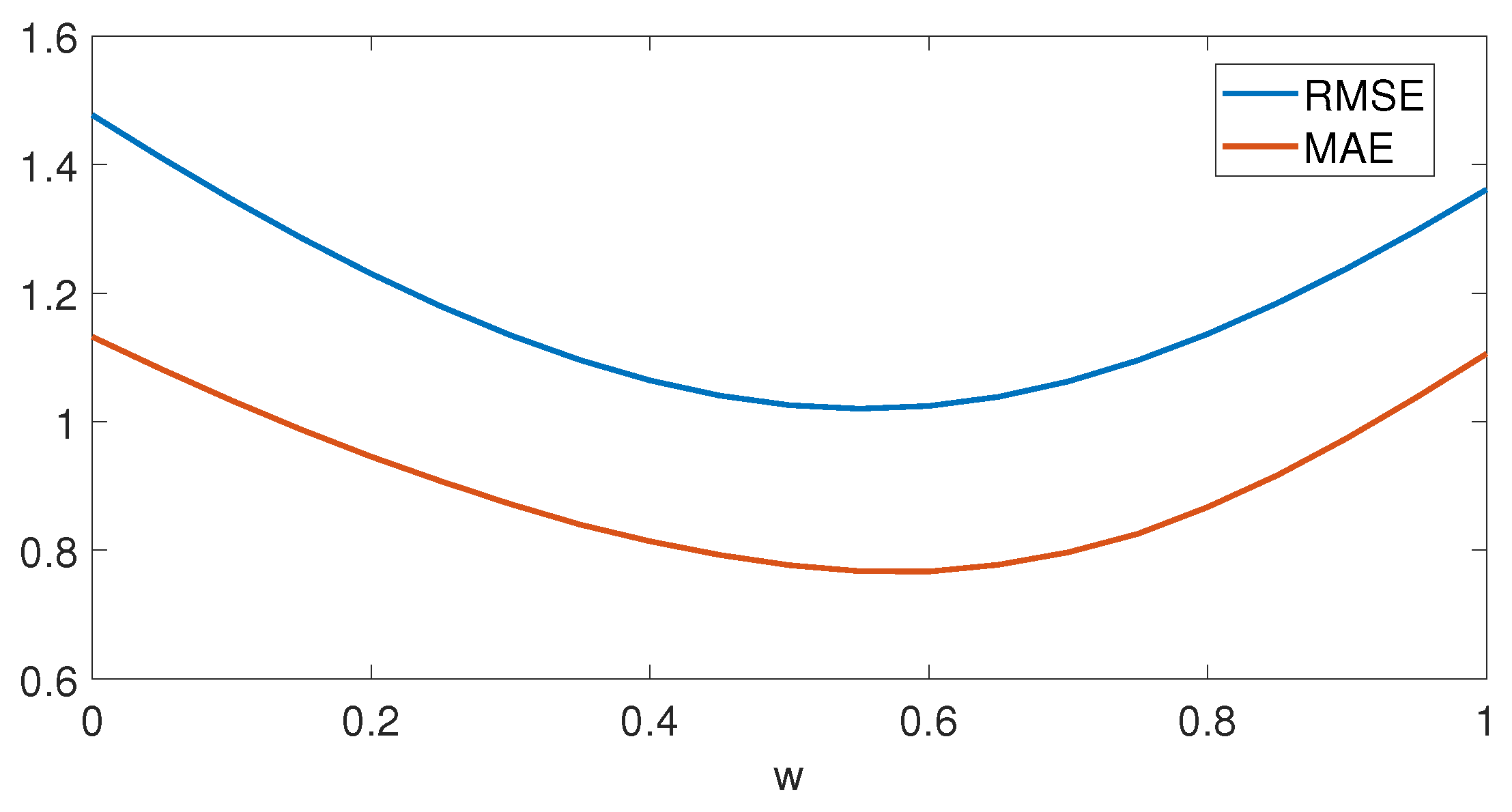
Finally, to systematically evaluate the impact of the weighting coefficient w utilized in in the flood depth estimation stage, and introduced in Equation (10), a parameter sensitivity analysis was conducted across all 12 catchments of the dataset. The primary purpose of the weight w is to regulate the operational balance between the physically conservative maximum boundary elevation estimate ($H_{max}$) and the statistically representative mean boundary elevation estimate ($H_{mean}$). Because unsupervised horizontal edge delineation can be susceptible to localized topographic anomalies or minor boundary misclassifications, tuning this parameter controls the model’s sensitivity to outlier elevation values along the extracted perimeters.

In our core framework, we empirically selected a balanced baseline value of $w=0.5$. This setting dictates that both depth components contribute equally to the final volumetric floodwater profile, serving as a neutral weighting scheme that balances the absolute physical upper bound with the average terrain elevation of the boundary, thereby maintaining the strictly unsupervised nature of our method.

As illustrated by the sensitivity curves in Figure 9, varying w from 0 to 1 directly alters the global performance, with the minima of the RMSE and MAE curves representing the mathematically optimal configurations for this specific dataset. Crucially, in our proposed framework, $w=0.5$ is established as a fixed a priori parameter. It functions as a neutral arithmetic mean that balances the physical upper bound with the average boundary terrain. Selecting this parameter without prior exposure to the data preserves the strictly unsupervised, training-free nature of the methodology. Therefore, this sensitivity analysis serves strictly as a post-hoc validation rather than a tuning mechanism. The relatively shallow gradients of the error curves around this baseline demonstrate that our framework is highly stable and resilient to parameter perturbations. The proximity of our fixed prior ($w=0.5$) to the empirical minima validates the robustness of this neutral weighting scheme for deployment in unmapped environments, effectively bypassing the need for training data or site-specific calibration.

6.5. Topological and Morphological Drivers of Depth Error

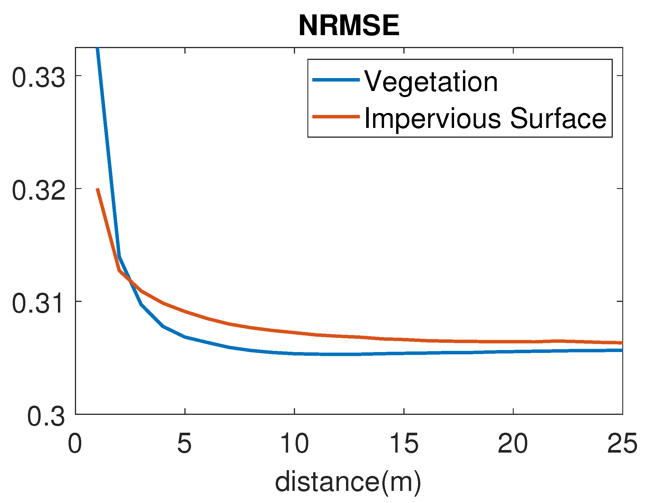
While the previous sections qualitatively established the relationship between boundary sampling and hydrostatic fidelity, this subsection provides a rigorous quantitative evaluation of the spatial and morphological drivers of depth error. We first investigate how the relative error distribution correlates with physical landscape features. Figure 10 illustrates the behavior of the maximum-normalized RMSE (nRMSE) as a function of the spatial distance from two distinct land cover boundaries, namely vegetation (blue curve) and impervious surfaces (red curve). The analysis reveals a pronounced, non-linear spatial decay in depth estimation error. The highest error magnitudes, peaking at over 0.33 for vegetation and 0.32 for impervious surfaces, reveal that vegetation exerts a more pronounced negative effect on depth accuracy. This is physically plausible, considering that tree canopies, especially in dense clusters, can occlude the underlying floodwater.

Furthermore, these high error magnitudes are heavily concentrated within the first two to five meters of these structural borders. This sharp error spike at the immediate land-water interface quantitatively confirms that residual micro-topographic artifacts, such as imperfectly filtered building footprints or dense root systems in the underlying DTM, disproportionately skew the baseline elevations sampled by the algorithm. Conversely, as the distance from these boundaries increases beyond 10 m, the nRMSE rapidly drops and stabilizes into a steady low-error plateau across the open water interior. This spatial error distribution provides compelling quantitative proof that the framework achieves high hydrostatic accuracy in unobstructed terrain, and that the aggregated regional depth errors are intrinsically driven by localized topographic complexities at the sampling boundaries.

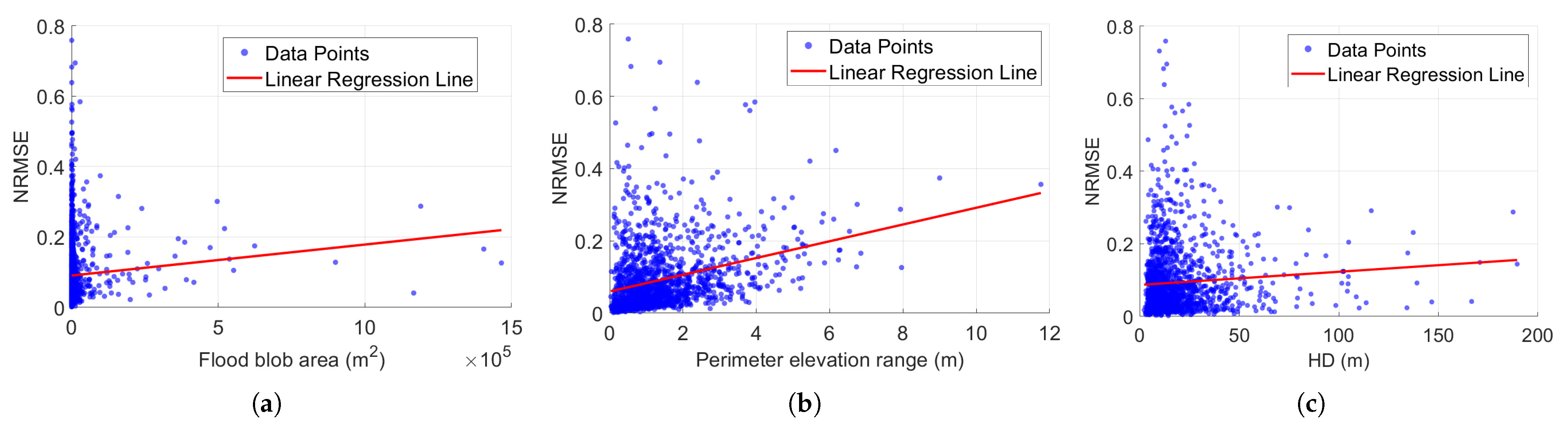
To further address the potential for slope-driven bias and to quantitatively assess the relationship between 2D spatial metrics and 3D depth fidelity, we analyzed the Pearson correlation between the maximum-normalized RMSE (nRMSE) and three distinct physical variables across the extracted flood components (see Figure 11). First, we evaluated whether depth error is systematically influenced by the spatial scale of the inundation by comparing nRMSE against individual flood component (blob) area. The scatter plot and corresponding linear regression line (red) in Figure 11a indicate that while vastly larger contiguous water bodies might introduce slightly higher variance due to extended hydrostatic baselines, the raw size of the flood component is not a primary driver of depth error. This observation is mathematically supported by the weak positive correlation ($r=0.2998$).

Next, we tested the hypothesis that high perimeter elevation ranges, which are indicative of steep topographic slopes (e.g., proximity to a channel), inherently bias depth estimations. As shown in Figure 11b, the correlation between perimeter elevation range and nRMSE is negligible ($r=0.0824$). This exceptionally low correlation effectively rules out systematic slope-driven bias, demonstrating that the framework’s hydrostatic anchoring remains highly stable regardless of the absolute topographic relief spanned by the flood boundary. However, it must be noted that the perimeter elevation ranges encountered are generally small. In hypothetical cases where a single continuous boundary presents severe elevation discrepancies, the fundamental physical assumption of hydrostatic equilibrium would no longer hold, falling outside the theoretical scope of this study.

Finally, to quantitatively validate our central empirical claim that overall depth error is governed by localized topographic sampling rather than raw global segmentation degradation, we evaluated nRMSE against a boundary-specific spatial error metric: the Hausdorff Distance (Figure 11c). The Hausdorff Distance measures the maximum spatial deviation between the predicted 2D boundary and the ground truth waterline. Crucially, the Pearson correlation between these spatial boundary shifts and the resulting 3D depth error is virtually nonexistent ($r=0.0720$). This near-zero correlation provides definitive mathematical proof for our earlier qualitative observations. Specifically, a massive horizontal boundary misalignment (high Hausdorff Distance) occurring over flat, unflooded terrain will introduce negligible hydrostatic elevation error. Conversely, minor horizontal misalignments that coincidentally align with steep micro-topographic anomalies can severely skew the localized hydrostatic plane. Consequently, these metrics quantitatively confirm that the severity of the depth error is not a linear product of 2D boundary displacement, but rather an artifact of the specific topographic gradients sampled at those offset margins.

6.6. Comparative Evaluation

To comprehensively quantify the predictive performance of our proposed framework on the given dataset, we conducted a three-fold analysis: first, we validated our approach against the isolated depth estimation module using ground truth extent masks; second, we investigated two optimization-based baseline methods; and finally, we benchmarked our results against the FloodWater Depth Estimation Tool [40,47].

In order to quantify the relative performance of our framework compared to these methods, we utilize a closeness metric, ${\eta }_{baseline}$, formulated as the percentage ratio of the baseline RMSE to the proposed RMSE:

$${\eta }_{baseline}=100\times {\displaystyle \frac{{\mathrm{RMSE}}_{baseline}}{{\mathrm{RMSE}}_{proposed}}}$$

(16)

Under this convention, values below 100% indicate a performance deficit relative to the baseline model. Such values are expected, as the proposed unsupervised framework is being compared against configurations that explicitly utilize actual ground truth flood extent and/or depth data. However, values closely approaching or exceeding 100% (which denote a performance gain achieved by our method despite lacking prior calibration) highlight the robust predictive capability of the proposed framework. The complete quantitative results across all benchmarked methods are summarized in

Table 4. Comparative evaluation of the proposed framework against the depth estimation module in isolation using ground truth flood extent masks (TE-Proposed), PSO baselines utilizing ground truth depth masks with our unsupervised flood extents (AE-PSO) and the true extents (TE-PSO), and the Floodwater Depth Estimation Tool [40,47] with our auto-extracted extents (AE-FwDET) and true extents (TE-FwDET) across the 12 study sites, sorted in ascending order of maximum-normalized RMSE (nRMSE). The table reports the absolute RMSE (in meters) for all methods, alongside the corresponding relative performance changes $\eta$ to quantify how closely our Proposed and TE-Proposed frameworks perform relative to their respective baselines.

Site	Proposed		TE-Proposed		AE-PSO		TE-PSO		AE-FwDET		TE-FwDET
	nRMSE ↓	RMSE ↓	RMSE ↓	$\mathit{\eta }$ (%) ↑	RMSE ↓	$\mathit{\eta }$ (%) ↑	RMSE ↓	$\mathit{\eta }$ (%) ↑	RMSE ↓	$\mathit{\eta }$ (%) ↑	RMSE ↓	$\mathit{\eta }$ (%) ↑
Princeville	0.1376	0.9664	0.8176	84.61%	0.8899	92.08%	0.7495	91.66%	1.7492	181.00%	1.7623	215.53%
Goldsboro1	0.1553	1.1085	1.6661	150.30%	0.9867	89.01%	1.0092	60.57%	1.4918	134.58%	1.4980	89.91%
HancheysStore	0.1672	0.9326	0.8924	95.69%	0.9188	98.52%	0.8754	98.10%	1.7237	184.83%	1.7169	192.40%
Chinquaqin	0.1698	0.4912	0.4185	85.20%	0.4456	90.72%	0.3467	82.84%	0.9504	193.49%	0.9388	224.32%
Lumberton	0.1700	1.1811	1.4671	124.21%	0.9703	82.15%	0.8696	59.27%	1.6797	142.21%	1.6855	114.89%
Nichols	0.1715	0.1649	0.1230	74.60%	0.1625	98.54%	0.1129	91.80%	0.3185	193.15%	0.3213	261.18%
Greenville1	0.1807	0.6260	0.4935	78.83%	0.4781	76.37%	0.2166	43.90%	1.0646	170.06%	1.0144	205.56%
Kinston1	0.1811	1.5823	2.5118	158.74%	1.4218	89.86%	1.0673	42.49%	1.9355	122.32%	1.8664	74.31%
Kinston2	0.1882	0.8942	0.6816	76.22%	0.8296	92.78%	0.5807	85.20%	1.3202	147.64%	1.3088	192.03%
Greenville2	0.1892	1.1572	1.4446	124.84%	1.1106	95.97%	1.2462	86.27%	1.8926	163.55%	1.9087	132.13%
Wallace	0.2241	0.9119	0.7492	82.16%	0.9387	102.94%	0.7848	104.75%	1.2445	136.47%	1.2118	161.75%
Goldsboro2	0.2514	1.6861	1.4987	88.89%	1.5905	94.33%	0.9164	61.15%	1.9711	116.90%	1.8376	122.61%

.

6.6.1. Isolated Depth Estimation Module (TE-Proposed)

To evaluate our depth estimation module in isolation from the 2D segmentation stage, we introduce the following evaluation configuration: True-Extent-Proposed (TE-Proposed). This approach feeds the ground truth flood extent masks directly into our proposed unsupervised depth estimation algorithm, as described in Section 4.2. This completely eliminates boundary-driven omission and commission errors, allowing us to strictly assess the raw efficacy of our heuristic boundary sampling and localized hydrostatic anchoring without the cascading influence of prior segmentation inaccuracies. The resulting quantitative data are reported in Table 4, columns 4–5.

By comparing the fully unsupervised pipeline against the TE-Proposed configuration, we observe a counterintuitive but highly revealing dynamic. As expected, in catchments hindered by massive 2D omission errors, such as Kinston2 (Recall = 0.6330) and Goldsboro2 (Recall = 0.4935), applying the true boundary improves the depth estimation, yielding $\eta$ values of 76.22% and 88.89%, respectively. However, across a significant portion of the dataset, most notably Goldsboro1 ($\eta =150.30\%$), Lumberton ($\eta =124.21\%$), Kinston1 ($\eta =158.74\%$), and Greenville2 ($\eta =124.84\%$), the proposed unsupervised pipeline drastically outperforms the ground truth baseline.

As established in the preceding analysis, this is a direct consequence of the dataset’s temporal misalignment. Consequently, feeding peak boundaries into the heuristic model forces it to sample elevations at the extreme outer margins of the floodplain, which frequently coincide with complex physical structures (e.g., steep channel banks, dense canopies, or urban infrastructure) where residual LiDAR artifacts in the DTM are most severe. Conversely, the unsupervised segmentation maps the temporally synchronous, receded waterline visible in the post-event imagery. By naturally stopping short of these elevated, artifact-heavy historical boundaries, the unsupervised mask inadvertently acts as a spatial buffer, sampling interior DTM pixels that are closer to true bare-earth elevations. Ultimately, this isolated evaluation definitively proves that forcing alignment to temporally offset peak ground truths can paradoxically degrade 3D depth accuracy, and that achieving maximum hydrostatic fidelity relies heavily on sampling topologically sound, artifact-free terrain.

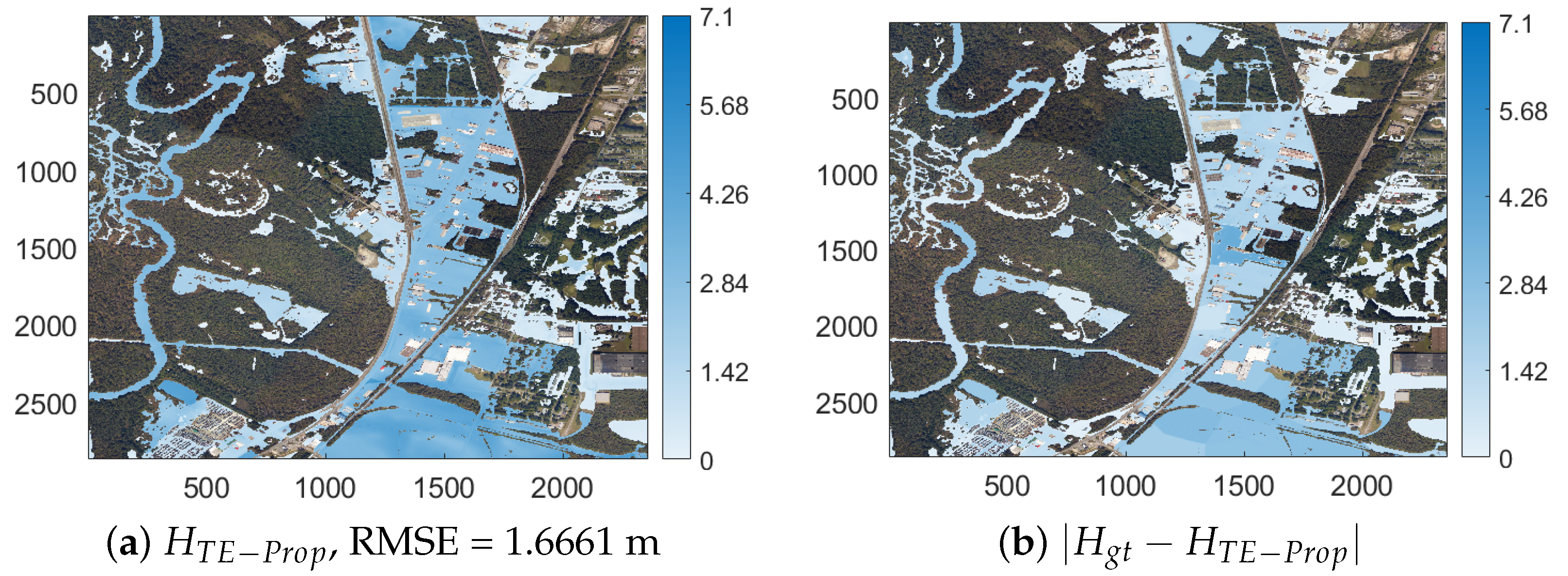
A qualitative illustration of this phenomenon is presented in Figure 12. This builds upon the previous analysis of Goldsboro1 in Figure 6, which depicted the RGB imagery, the ground truth depth map $H_{gt}$, the proposed framework’s fully unsupervised depth prediction H, and the absolute error map $|H_{gt}-H|$ in (e), (f), (g), and (h), respectively. Here, Figure 12a,b illustrate the isolated proposed depth from the isolated depth estimation module when fed with the ground truth extent ($H_{TE-Prop}$), alongside its corresponding absolute error map $|H_{gt}-H_{TE-Prop}|$.

As observed in the error map (Figure 12b), forcing the depth estimation module to anchor strictly to the exact ground truth boundaries introduces severe, widespread depth overestimations across large portions of the catchment. While the unsupervised method’s inherent slight under-segmentation (Figure 6g) safely buffered the sampling pixels away from structural edges, the true boundaries frequently align with complex terrain features such as dense vegetation and steep embankments. A clear visual example of this behavior occurs in the lower-middle section of the catchment (Figure 6e), where dense vegetation visually fragments the floodwater into approximately four distinct spatial components. The ground truth mask (Figure 6f), however, aggregates this area into a massive, heavily contiguous inundation body.

By naturally excluding these vegetated occlusions, the proposed unsupervised method partitions the water into multiple isolated components. This critical localization allows the depth module to calculate independent, highly localized elevation constants for each sub-region, yielding an overall RMSE of 1.1085 m. Conversely, supplying the module with the continuous ground truth mask forces the algorithm to calculate a shared elevation constant over a vastly expanded area. This forced spatial aggregation severely strains the localized hydrostatic equilibrium assumption. Coupled with the sampling of topographically noisy DTM pixels at the true outer margins, this artificially inflates the regional hydrostatic elevation constant, propagating a heavy error penalty throughout the entire contiguous water body and ultimately yielding a significantly higher overall error (RMSE = 1.6661 m).

6.6.2. Optimization-Based Baselines (AE-PSO and TE-PSO)

The optimization-based baselines operate on the same multimodal input data but leverage ground truth depth profiles to calibrate and optimize the model parameters using Particle Swarm Optimization (PSO) [48,49,50]. PSO is a population-based metaheuristic algorithm that solves complex optimization problems by iteratively improving a swarm of candidate solutions. In the context of this study, for each isolated flooded region (blob), the swarm explores the continuous parameter space of potential elevation constants ($c_i$), dynamically converging on the precise value that minimizes the RMSE between the simulated hydrostatic depth and the actual ground truth measurements. This ensures that the PSO baselines represent the optimally calibrated performance of the rigid, single-constant hydrostatic model (Equation (5)) under their respective boundary conditions.

The specific optimization baseline configurations are defined as follows:

• Auto-Extent-PSO (AE-PSO): To assess the practical applicability and comparative performance of the proposed hydrostatic model formalized in Equation (10), this baseline utilizes our automatically derived, unsupervised flood extent masks. By relying on the predicted boundaries but optimizing the elevation constant via PSO, this configuration isolates the performance of our heuristic vertical anchoring against an optimized terrain-mapping counterpart.
• True-Extent-PSO (TE-PSO): To isolate the error inherited strictly from the hydrostatic assumption, this baseline substitutes the estimated flood extent mask with the ground truth flood extent mask. Combined with the PSO-driven parameter estimation, TE-PSO represents the optimally calibrated performance of the single-constant hydrostatic model for this dataset.

Table 4 (columns 6–9) contextualizes the depth estimation accuracy of our proposed framework against the two computationally intensive PSO baselines, AE-PSO and TE-PSO. By comparing the proposed framework to AE-PSO, we isolate the performance of our heuristic vertical anchoring against an optimized terrain-mapping counterpart. As demonstrated by the corresponding AE-PSO $\eta$ metric (column 7), the proposed uncalibrated framework operates within a tight 10% of the optimized baseline’s performance in eight of the twelve sites. Furthermore, in environments like Wallace, where the auto-extent comprises massive but porous flood components, our localized sampling approach actually outperforms the globally optimized baseline by 2.94%. These results confirm that the proposed computationally lightweight, heuristic-based depth mapping is highly efficient and performs on par with this intensive calibration method.

Evaluating our TE-Proposed pipeline against the “ideal” TE-PSO scenario (Table 4, columns 4, 8, and 9) provides a direct comparison by standardizing the input boundaries to the exact ground truth. This isolates the efficacy of our heuristic vertical anchoring against a fully calibrated optimization. In catchments where the true peak boundaries intersect complex physical structures, such as Kinston1, Greenville1, and Lumberton, the heuristic approach exhibits a pronounced performance gap, as indicated by $\eta$ values of 42.49%, 43.90%, and 59.27%, respectively. As established in our qualitative analysis above, forcing the heuristic model to sample elevations at the extreme outer margins of potential artifact-heavy DTMs artificially inflates the hydrostatic constant. The TE-PSO avoids this geometric trap entirely by fitting its parameters directly to the 3D ground truth depth, yielding a superior RMSE.

However, when the true boundaries align with clean, topologically sound terrain, the uncalibrated heuristic model proves exceptionally competitive. In sites like HancheysStore ($\eta$ = 98.10%), Nichols ($\eta$ = 91.80%), and Princeville ($\eta$ = 91.66%), the proposed framework operates at near parity with the fully optimized baseline. Remarkably, in Wallace, the TE-Proposed configuration actually surpasses the optimally calibrated TE-PSO baseline by 4.75%. While TE-PSO minimizes a global mathematical error across massive contiguous water bodies, which can skew the elevation constant to accommodate deep-channel outliers, the heuristic approach strictly anchors to the physical topography of the complex waterline. Ultimately, these findings demonstrate that our localized, topography-driven anchoring is not merely a computationally cheap approximation, but a physically grounded strategy that can actively prevent the spatial over-fitting inherent to globally optimized baselines.

6.6.3. Floodwater Depth Estimation Tool (FwDET)

Finally, we utilized the Floodwater Depth Estimation Tool (FwDET) [40,47] to establish two additional baseline configurations: AE-FwDET (using our unsupervised flood extents) and TE-FwDET (using the ground truth extents). To ensure a rigorous comparison, we employed the latest version of the algorithm (v2.1), which introduces a boundary cell smoothing and filtering procedure to improve the tool’s accuracy, executed via its official QGIS processing script (Available at: https://github.com/csdms-contrib/fwdet/tree/master/qgis_port (accessed on 3 August 2026)) within QGIS version 3.34.5 (https://www.qgis.org/ (accessed on 3 August 2026)), the environment against which the tool was actively tested. Following the optimal parameter recommendations for high-resolution DEMs established by [47], the algorithm was configured with 10 smoothing iterations and a slope threshold of 0.5%. To ensure a fair computational comparison, FwDET was provided with the identical 1 m resolution DTMs used by our method. Under these conditions, FwDET’s execution was significantly slower, with processing times ranging from 66.22 to 420.68 s per site. On average, FwDET required 127.60 s strictly for depth calculation, in stark contrast to our framework’s average of 8.83 s, a time that remarkably encompasses both the initial 2D semantic segmentation and the subsequent 3D depth estimation stages.

Evaluating the proposed unsupervised framework against the AE-FwDET baseline (Table 4, columns 3, 10, and 11) reveals a striking performance disparity. The proposed framework drastically outperforms FwDET across all 12 catchments, yielding $\eta$ values ranging from 116.90% (Goldsboro2) to an overwhelming 193.49% (Chinquaqin). Furthermore, comparing the TE-Proposed configuration to the TE-FwDET baseline (Table 4, columns 4, 12, and 13), where the depth calculation algorithms use true-extent boundaries, our heuristic localized approach vastly outpaces FwDET in 10 of the 12 sites. Most notably in Nichols, the TE-Proposed framework achieves an $\eta$ of 261.18%.

This systemic underperformance by FwDET is a direct consequence of operating on a high-resolution 1 m DTM. As acknowledged in prior literature [40], FwDET fundamentally relies on calculating depth by assigning the elevation of the nearest boundary grid cell (via Euclidean distance) to the interior flooded pixels. While this nearest-neighbor allocation functions adequately on coarse 10 m DEMs, where terrain features are naturally blurred, a 1 m DTM captures sharp micro-topography, such as steep riverbanks, raised roadbeds, and localized embankments. When the boundary mask inevitably intersects these high-elevation artifacts, or conversely, when boundaries extend into local depressions, FwDET blindly propagates these extreme high or low elevation values deep into the floodplain, creating massive, artificial depth errors. Conversely, our proposed framework utilizes a localized hydrostatic anchoring and a continuous spatial smoothing kernel (Equation (11)), which effectively dampens these micro-topographic anomalies and preserves a physically realistic water surface. Interestingly, TE-FwDET registers lower absolute errors than TE-Proposed in only two catchments, Kinston1 ($\eta$ = 74.31%) and Goldsboro1 ($\eta$ = 89.91%).

The disparity is qualitatively illustrated in Figure 13, displaying the Nichols catchment in the first two columns and the Kinston1 catchment in the last two. In the Nichols catchment, the proposed method (Figure 13e) performs almost twice as well as the AE-FwDET baseline (RMSE of 0.1649 m vs. 0.3185 m), yielding a highly accurate depth map and significantly lower absolute errors than its counterpart (Figure 13f and Figure 13j, respectively), by cleanly anchoring to the true topography. In contrast, even with perfect boundaries, TE-FwDET (Figure 13q,r) introduces severe overestimations (RMSE = 0.3213 m) compared with TE-Proposed (RMSE = 0.1230 m, Figure 13m,n). Because FwDET calculates influence zones based on the single nearest boundary pixel, the resulting water surface exhibits unnatural, straight-line geometric transitions rather than conforming to hydrostatic equilibrium.

Conversely, for the Kinston1 catchment, our Auto-Extent-Proposed framework (RMSE = 1.5823 m, Figure 13g,h) outperforms its counterpart FwDET algorithm (RMSE = 1.9355 m, Figure 13k,l), but when introduced to true-extent borders, FwDET (RMSE = 1.8664 m, Figure 13s,t) bests our heuristic depth estimation method (RMSE = 2.5118 m, Figure 13o,p). Because our localized model is forced to anchor to these true, historical peak boundaries, it samples extreme DTM artifacts, heavily penalizing the resulting single-blob constant. FwDET’s heavy application of ten low-pass filtering iterations acts as a blunt mathematical instrument in these specific scenarios, artificially smoothing out the extreme boundary spikes at the cost of physical accuracy, thereby dampening the penalty. However, as evidenced by the broader dataset, when boundaries are clean and representative of the active waterline, our localized heuristic anchoring is definitively superior to FwDET’s distance-based allocation in high-resolution 1 m DTMs.

7. Conclusions and Future Work

This study introduced a fully unsupervised, training-free framework for rapid, standing floodwater depth estimation in urban and peri-urban environments by integrating post-event aerial imagery with Digital Terrain Models (DTMs). Operating without the bottleneck of manual annotations or task-specific training data, the proposed method addresses the complex spatial nature of flood dynamics by leveraging localized terrain constraints and the physical principle of hydrostatic equilibrium. Experimental validation across 12 heterogeneous catchments from the Inundation2Depth dataset [19] demonstrated regional spatial robustness. By automatically extracting operationally viable flood boundaries under clear optical conditions, eliminating the need for manual mask corrections, the framework yields spatially coherent and physically plausible depth estimates. Furthermore, our continuous, pixel-wise evaluation demonstrates that this approach offers a highly scalable and computationally efficient alternative to data-heavy supervised baselines, which often rely on sparse, point-based validation.

However, extensive experimental evaluation also establishes a critical architectural insight regarding multimodal sensor dependency: the performance of our training-free pipeline is structurally coupled with the baseline quality of the input aerial and LiDAR terrain-informed data. Because the geometric depth module relies on sampling topographic points exactly where the horizontal land-water interface is detected, any visual ambiguities in the optical imagery, such as structural building shadows, dense vegetation canopies, cloud cover, or a lack of spectral contrast in highly turbid waters, can cause substantial omission errors that directly dictate the positioning of the extraction boundary. Consequently, when interpreting the overall robustness of the framework, it is critical to acknowledge its strict dependency on optical visibility. Additionally, when these horizontal variances align with steep elevation gradients in the underlying DTM, they introduce artificial vertical references into the hydrostatic-based depth estimation module. Crucially, isolating the depth module revealed a counterintuitive dynamic: perfect 2D ground truth boundaries do not guarantee optimal 3D depth due to temporal misalignment. Because ground truth masks typically represent peak historical inundation, they force topographic sampling into elevated, artifact-heavy terrain. In contrast, our unsupervised approach maps the contemporaneous, receded waterline visible in post-event imagery, naturally buffering sampling pixels away from these noisy historical margins and often yielding more reliable depth estimates. Rather than exposing a flaw in the physical modeling phase, this dependency emphasizes that the optimization of unsupervised flood mapping is inherently bounded by the fidelity of the raw inputs, highlighting the necessity for high resolution, clear, and accurate data feeds during rapid disaster response mapping.

Finally, the physical validity of the derived depth maps is fundamentally constrained by the hydrostatic equilibrium assumption. While highly effective for stationary or slowly receding waters, the framework’s accuracy diminishes in dynamic hydraulic scenarios, such as fast-flowing flash floods over steep terrain or in urban basins experiencing active, localized mechanical drainage, which disrupt the assumed horizontal water surface. To address these physical limitations originating from applying a constant hydrostatic reference level over vast, 8-connected fluvial networks, future iterations of this framework will investigate spatially varying reference surfaces. Implementing a distance-weighted interpolation or a slope-fitted polynomial plane along the longitudinal axis of large connected components would allow the model to account for genuine downstream surface slopes, preventing the systematic depth biases that occur at the upstream and downstream extremities of active river channels.

While the current unsupervised paradigm delivers highly stable depth mapping across diverse urban and peri-urban terrain profiles, several avenues remain open for future investigation. A primary objective for subsequent research is transitioning this framework into an end-to-end unsupervised or self-supervised deep learning pipeline [51]. Instead of relying on a decoupled two-stage approach, neural networks could be designed to directly predict volumetric flood depth from raw multimodal inputs (RGB aerial or satellite imagery and DTMs) without requiring labeled ground truth data. One promising direction involves self-supervised contrastive learning or masked autoencoders [52] optimized for multi-source remote sensing data, where the model learns robust structural representations by masking and reconstructing paired RGB-DTM patches. Another crucial advancement would be the development of unsupervised physics-guided neural networks (PGNNs) [53]. By embedding hydrostatic equilibrium constraints and terrain elevation boundaries directly into the network’s loss function, the deep model could optimize its depth predictions autonomously. This end-to-end integration would enable the framework to learn complex spatial priors, gracefully handling micro-topographical architectural noise and dense canopy occlusions that traditionally challenge static geometric solvers.

To explicitly overcome the optical limitations, namely cloud occlusion, structural shadows, and spectral blending in highly turbid waters, future iterations of this framework must pivot toward multi-sensor fusion. Specifically, the integration of SAR data alongside optical imagery presents a highly actionable mitigation strategy. Because SAR systems operate independently of solar illumination and penetrate dense cloud cover, fusing SAR-derived backscatter anomalies with optical segmentations would ensure robust, weather-agnostic boundary extraction. Furthermore, expanding the input pipeline to ingest broader multi-spectral data, particularly Near-Infrared (NIR) and Shortwave-Infrared (SWIR) bands, would allow the integration of advanced water indices. This multi-spectral feature fusion could effectively decouple turbid, sediment-heavy floodwaters from similarly colored urban backgrounds, significantly enhancing the resilience of the initial 2D delineation stage.

Beyond algorithmic advancements, future work must also address the inherent data scarcity constraints associated with acquiring synchronous, paired aerial imagery and high-fidelity DTMs for newly impacted geographic regions. While the current evaluation demonstrates strong regional transferability across the coastal and inland plains of the Carolinas, the framework’s global generalization remains untested. Future research must prioritize cross-region validation using datasets from distinct climatic and topographical biomes, as well as imagery from varied optical and active sensors, to rigorously define the operational boundaries of this unsupervised approach on a global scale. To mitigate this bottleneck, research will focus on generative synthetic data augmentation [54]. By synthetically co-generating diverse, simulated post-flood aerial textures aligned with varying artificial or real DTM structures, it becomes possible to simulate rare and extreme multi-meter inundation scenarios. Crucially, these rich synthetic environments can be leveraged to train multimodal deep neural architectures that ingest both RGB imagery and topographic streams simultaneously. This synthetic training pipeline will facilitate extensive domain generalization studies, ultimately helping to robustly close the gap for downstream data-driven flood management models without the need for human annotated real world records.

References

1. Mishra, A.; Mukherjee, S.; Merz, B.; Singh, V.P.; Wright, D.B.; Villarini, G.; Paul, S.; Kumar, D.N.; Khedun, C.P.; Niyogi, D.; et al. An overview of flood concepts, challenges, and future directions. J. Hydrol. Eng. 2022, 27, 03122001. [Google Scholar] [CrossRef]
2. Blay, J.; Hashemi-Beni, L. Advanced Geo-Data Analytics and AI for 3D Flood Mapping to Protect Built Assets. Isprs Ann. Photogramm. Remote Sens. Spat. Inf. Sci. 2025, X-G-2025, 159–164. [Google Scholar] [CrossRef]
3. Drakonakis, G.I.; Tsagkatakis, G.; Fotiadou, K.; Tsakalides, P. OmbriaNet—supervised flood mapping via convolutional neural networks using multitemporal sentinel-1 and sentinel-2 data fusion. IEEE J. Sel. Top. Appl. Earth Obs. Remote Sens. 2022, 15, 2341–2356. [Google Scholar] [CrossRef]
4. Dong, Z.; Liang, Z.; Wang, G.; Amankwah, S.O.Y.; Feng, D.; Wei, X.; Duan, Z. Mapping inundation extents in Poyang Lake area using Sentinel-1 data and transformer-based change detection method. J. Hydrol. 2023, 620, 129455. [Google Scholar] [CrossRef]
5. He, Y.; Wang, J.; Zhang, Y.; Liao, C. An efficient urban flood mapping framework towards disaster response driven by weakly supervised semantic segmentation with decoupled training samples. ISPRS J. Photogramm. Remote Sens. 2024, 207, 338–358. [Google Scholar] [CrossRef]
6. Simantiris, G.; Panagiotakis, C. Unsupervised color-based flood segmentation in UAV imagery. Remote Sens. 2024, 16, 2126. [Google Scholar] [CrossRef]
7. Rahnemoonfar, M.; Chowdhury, T.; Sarkar, A.; Varshney, D.; Yari, M.; Murphy, R.R. Floodnet: A high resolution aerial imagery dataset for post flood scene understanding. IEEE Access 2021, 9, 89644–89654. [Google Scholar] [CrossRef]
8. Wieland, M.; Martinis, S.; Kiefl, R.; Gstaiger, V. Semantic segmentation of water bodies in very high-resolution satellite and aerial images. Remote Sens. Environ. 2023, 287, 113452. [Google Scholar] [CrossRef]
9. Simantiris, G.; Bacharidis, K.; Papanikolaou, A.; Giannakakis, P.; Panagiotakis, C. AIFloodSense: A Global Aerial Imagery Dataset for Semantic Segmentation and Understanding of Flooded Environments. Remote Sens. 2026, 18, 938. [Google Scholar] [CrossRef]
10. San Jose, I.K.; Wiguna, S.; Kametaka, R.; Adriano, B.; Mas, E.; Koshimura, S. Evaluation of open-source SAR-based flood datasets for flood extent mapping in emergency settings. Prog. Disaster Sci. 2026, 29, 100507. [Google Scholar] [CrossRef]
11. Van Der Knijff, J.; Younis, J.; De Roo, A. LISFLOOD: A GIS-based distributed model for river basin scale water balance and flood simulation. Int. J. Geogr. Inf. Sci. 2010, 24, 189–212. [Google Scholar] [CrossRef]
12. Tian, M.; Sun, H.; Yang, G.; Wei, E.; Fang, P.; Sun, S. Research on flood disaster monitoring and early warning system integrating three-dimensional geographic information and numerical simulation. In IET Conference Proceedings CP941; The Institution of Engineering and Technology: Stevenage, UK, 2025; Volume 2025, pp. 69–75. [Google Scholar]
13. Patro, S.; Chatterjee, C.; Mohanty, S.; Singh, R.; Raghuwanshi, N. Flood inundation modeling using MIKE FLOOD and remote sensing data. J. Indian Soc. Remote Sens. 2009, 37, 107–118. [Google Scholar] [CrossRef]
14. Dang, T.Q.; Tran, B.H.; Le, Q.N.; Dang, T.D.; Tanim, A.H.; Pham, Q.B.; Bui, V.H.; Mai, S.T.; Thanh, P.N.; Anh, D.T. Application of machine learning-based surrogate models for urban flood depth modeling in Ho Chi Minh City, Vietnam. Appl. Soft Comput. 2024, 150, 111031. [Google Scholar] [CrossRef]
15. Zhang, X.; Xiao, Y.; Zhu, J.; Cheng, W.; Zhang, Y. Flood Risk Assessment and Management Strategies under Extreme Frequency Events. Water Resour. Manag. 2026, 40, 340. [Google Scholar] [CrossRef]
16. Liu, B.; Li, Y.; Ma, M.; Mao, B. A comprehensive review of machine learning approaches for flood depth estimation: Liu et al. machine learning approaches for flood depth estimation. Int. J. Disaster Risk Sci. 2025, 16, 433–445. [Google Scholar] [CrossRef]
17. Elkhrachy, I. Flash flood water depth estimation using SAR images, digital elevation models, and machine learning algorithms. Remote Sens. 2022, 14, 440. [Google Scholar] [CrossRef]
18. Blay, J.; Hashemi-Beni, L. Geospatial and Deep Learning Approaches for Modeling Floodwater Depth in Urbanized Areas. Remote Sens. 2025, 18, 60. [Google Scholar] [CrossRef]
19. Blay, J.; Gebregziabher, Y.; Jha, M.K.; Beni, L.H. Inundation2Depth: A multi-source dataset for floodwater depth estimation in urban areas. Data Brief. 2025, 64, 112347. [Google Scholar] [PubMed]
20. Destefanis, T.; Guliyeva, S.; Boccardo, P.; Fissore, V. Advancing flood detection and mapping: A review of earth observation services, 3D data integration, and AI-Based techniques. Remote Sens. 2025, 17, 2943. [Google Scholar] [CrossRef]
21. Kharazi, B.A.; Behzadan, A.H. Flood depth mapping in street photos with image processing and deep neural networks. Comput. Environ. Urban Syst. 2021, 88, 101628. [Google Scholar] [CrossRef]
22. Song, Z.; Tuo, Y. Automated flood depth estimates from online traffic sign images: Explorations of a convolutional neural network-based method. Sensors 2021, 21, 5614. [Google Scholar] [CrossRef] [PubMed]
23. Alizadeh, B.; Behzadan, A.H. Scalable flood inundation mapping using deep convolutional networks and traffic signage. Comput. Urban Sci. 2023, 3, 17. [Google Scholar] [CrossRef]
24. Zhong, P.; Liu, Y.; Zheng, H.; Zhao, J. Detection of urban flood inundation from traffic images using deep learning methods. Water Resour. Manag. 2024, 38, 287–301. [Google Scholar] [CrossRef]
25. Liu, B.; Li, Y.; Feng, X.; Lian, P. BEW-YOLOv8: A deep learning model for multi-scene and multi-scale flood depth estimation. J. Hydrol. 2024, 645, 132139. [Google Scholar] [CrossRef]
26. Mishra, M.; Albano, R. FLOOD-DEPTH-ML: Machine Learning-Driven Python Application for Estimation of Urban Flood Depths through Submerged Vehicles Detection. Results Eng. 2026, 29, 109495. [Google Scholar] [CrossRef]
27. Du, W.; Qian, M.; He, S.; Xu, L.; Zhang, X.; Huang, M.; Chen, N. An improved ResNet method for urban flooding water depth estimation from social media images. Measurement 2025, 242, 116114. [Google Scholar] [CrossRef]
28. Wu, L.; Liu, Y.; Zhang, J.; Zhang, B.; Wang, Z.; Tong, J.; Li, M.; Zhang, A. Identification of flood depth levels in urban waterlogging disaster caused by rainstorm using a CBAM-improved ResNet50. Expert Syst. Appl. 2024, 255, 124382. [Google Scholar] [CrossRef]
29. Notarangelo, N.M.; Wirion, C.; van Winsen, F. STURM-FloodDepth: A deep learning pipeline for mapping urban flood depth using street-level and oblique aerial imagery. Geomatica 2025, 77, 100061. [Google Scholar] [CrossRef]
30. Meng, Z.; Peng, B.; Huang, Q. Flood depth estimation from web images. In Proceedings of the 2nd ACM SIGSPATIAL International Workshop on Advances on Resilient and Intelligent Cities, Chicago, IL, USA, 5 November 2019; pp. 37–40. [Google Scholar]
31. Li, J.; Cai, R.; Tan, Y.; Zhou, H.; Sadick, A.M.; Shou, W.; Wang, X. Automatic detection of actual water depth of urban floods from social media images. Measurement 2023, 216, 112891. [Google Scholar] [CrossRef]
32. Zou, B.; Peng, B.; Huang, Q. Flood Depth Assessment with Location-Based Social Network Data and Google Street View-A Case Study with Buildings as Reference Objects. In Proceedings of the IGARSS 2022-2022 IEEE International Geoscience and Remote Sensing Symposium; IEEE: New York, NY, USA, 2022; pp. 1344–1347. [Google Scholar]
33. Akinboyewa, T.; Ning, H.; Lessani, M.N.; Li, Z. Automated floodwater depth estimation using large multimodal model for rapid flood mapping. Comput. Urban Sci. 2024, 4, 12. [Google Scholar] [CrossRef]
34. Fuad, N.; Qian, X. LLM-Powered Flood Depth Estimation from Social Media Imagery: A Vision-Language Model Framework with Mechanistic Interpretability for Transportation Resilience. arXiv 2026, arXiv:2603.17108. [Google Scholar]
35. Lyu, H.; Zhou, S.; Wang, Z.; Fu, G.; Zhang, C. Assessing large multimodal models for urban floodwater depth estimation. Water Resour. Res. 2025, 61, e2024WR039494. [Google Scholar] [CrossRef]
36. Löwe, R.; Böhm, J.; Jensen, D.G.; Leandro, J.; Rasmussen, S.H. U-FLOOD–Topographic deep learning for predicting urban pluvial flood water depth. J. Hydrol. 2021, 603, 126898. [Google Scholar] [CrossRef]
37. Gebrehiwot, A.A.; Hashemi-Beni, L. Three-dimensional inundation mapping using UAV image segmentation and digital surface model. ISPRS Int. J. Geo-Inf. 2021, 10, 144. [Google Scholar] [CrossRef]
38. Do Lago, C.A.; Giacomoni, M.H.; Bentivoglio, R.; Taormina, R.; Junior, M.N.G.; Mendiondo, E.M. Generalizing rapid flood predictions to unseen urban catchments with conditional generative adversarial networks. J. Hydrol. 2023, 618, 129276. [Google Scholar] [CrossRef]
39. Wienhold, K.J.; Li, D.; Li, W.; Fang, Z.N. Flood inundation and depth mapping using unmanned aerial vehicles combined with high-resolution multispectral imagery. Hydrology 2023, 10, 158. [Google Scholar] [CrossRef]
40. Cohen, S.; Raney, A.; Munasinghe, D.; Loftis, J.D.; Molthan, A.; Bell, J.; Rogers, L.; Galantowicz, J.; Brakenridge, G.R.; Kettner, A.J.; et al. The Floodwater Depth Estimation Tool (FwDET v2. 0) for improved remote sensing analysis of coastal flooding. Nat. Hazards Earth Syst. Sci. 2019, 19, 2053–2065. [Google Scholar] [CrossRef]
41. Bendig, J.; Yu, K.; Aasen, H.; Bolten, A.; Bennertz, S.; Broscheit, J.; Gnyp, M.L.; Bareth, G. Combining UAV-based plant height from crop surface models, visible, and near infrared vegetation indices for biomass monitoring in barley. Int. J. Appl. Earth Obs. Geoinf. 2015, 39, 79–87. [Google Scholar] [CrossRef]
42. Colorimetry-Part 4: CIE 1976 L*a*b* Colour Space. Available online: https://cie.co.at/publications/colorimetry-part-4-cie-1976-lab-colour-space-0 (accessed on 3 August 2026).
43. Chavolla, E.; Zaldivar, D.; Cuevas, E.; Perez, M.A. Color spaces advantages and disadvantages in image color clustering segmentation. In Advances in Soft Computing and Machine Learning in Image Processing; Springer: Berlin/Heidelberg, Germany, 2018; pp. 3–22. [Google Scholar]
44. Canny, J. A computational approach to edge detection. IEEE Trans. Pattern Anal. Mach. Intell. 1986, PAMI-8, 679–698. [Google Scholar] [CrossRef]
45. Fabbri, R.; Costa, L.D.F.; Torelli, J.C.; Bruno, O.M. 2D Euclidean distance transform algorithms: A comparative survey. ACM Comput. Surv. 2008, 40, 1–44. [Google Scholar] [CrossRef]
46. Teng, J.; Jakeman, A.J.; Vaze, J.; Croke, B.F.; Dutta, D.; Kim, S. Flood inundation modelling: A review of methods, recent advances and uncertainty analysis. Environ. Model. Softw. 2017, 90, 201–216. [Google Scholar] [CrossRef]
47. Cohen, S.; Peter, B.G.; Haag, A.; Munasinghe, D.; Moragoda, N.; Narayanan, A.; May, S. Sensitivity of remote sensing floodwater depth calculation to boundary filtering and digital elevation model selections. Remote Sens. 2022, 14, 5313. [Google Scholar] [CrossRef]
48. Kennedy, J.; Eberhart, R. Particle swarm optimization. In Proceedings of ICNN’95-International Conference on Neural Networks; IEEE: New York, NY, USA, 1995; Volume 4, pp. 1942–1948. [Google Scholar]
49. Jain, M.; Saihjpal, V.; Singh, N.; Singh, S.B. An Overview of Variants and Advancements of PSO Algorithm. Appl. Sci. 2022, 12, 8392. [Google Scholar] [CrossRef]
50. Panagiotakis, C. Particle swarm optimization-based unconstrained polygonal fitting of 2d shapes. Algorithms 2024, 17, 25. [Google Scholar] [CrossRef]
51. Simantiris, G.; Panagiotakis, C. Unsupervised Deep Learning for Flood Segmentation in UAV imagery. In Proceedings of the International Conference on Pattern Recognition; Springer: Berlin/Heidelberg, Germany, 2024; pp. 408–423. [Google Scholar]
52. He, K.; Chen, X.; Xie, S.; Li, Y.; Dollár, P.; Girshick, R. Masked autoencoders are scalable vision learners. In Proceedings of the IEEE/CVF Conference on Computer Vision and Pattern Recognition, New Orleans, LA, USA, 18–24 June 2022; pp. 16000–16009. [Google Scholar]
53. Daw, A.; Karpatne, A.; Watkins, W.D.; Read, J.S.; Kumar, V. Physics-guided neural networks (pgnn): An application in lake temperature modeling. In Knowledge Guided Machine Learning; Chapman and Hall/CRC: Boca Raton, FL, USA, 2022; pp. 353–372. [Google Scholar]
54. Simantiris, G.; Bacharidis, K.; Panagiotakis, C. Closing the Domain Gap: Can Pseudo-Labels from Synthetic UAV Data Enable Real-World Flood Segmentation? Sensors 2025, 25, 3586. [Google Scholar] [CrossRef] [PubMed]
Figure 1. Schematic overview of the proposed automated floodwater depth estimation framework. The pipeline is divided into two primary phases: (1—blue arrow) unsupervised segmentation of high resolution aerial imagery to delineate the two-dimensional flood extent, and (2—orange arrows) integration of the extracted footprints with a Digital Terrain Model (DTM) to calculate the volumetric depth based on hydrostatic equilibrium.
Remotesensing 18 02673 g001
Figure 2. Blue and red curves correspond on the average value of (a) L, (b) A and (c) B color components computed on flood and background pixels respectively, for each image of the Inundation2Depth dataset [19], sorted in ascending order. The yellow curves show the corresponding Δ L , Δ A , and Δ B thresholds.
Remotesensing 18 02673 g002
Figure 3. Schematic overview of the unsupervised flood extent delineation pipeline detailed in Section 4.1. Initial exclusion masks (M) are derived from the input RGB imagery and corresponding CIELAB color space components. The composite mask ( M F i n a l ) is subsequently utilized in a spatial weighting process to estimate the dominant spectral signature of the floodwater. Finally, hysteresis thresholding is applied to the generated probability map to extract the definitive flood extent.
Remotesensing 18 02673 g003
Figure 4. (a) Schematic illustration of the DTM-based flood depth estimation principle. For any terrain point p ( x , y ) , the local flood depth is computed as the positive difference between the reference water surface elevation c i and the terrain elevation Z ( x , y ) . (b) Schematic representation of the proposed DTM-based flood depth estimation framework in a plan-view. The red line denotes the floodwater boundary, while the gray and blue color gradients illustrate the floodwater depth and the corresponding terrain elevation, respectively.
Remotesensing 18 02673 g004
Figure 5. Visual progression of the DTM-based flood depth estimation methodology. (a) Conservative depth estimate derived utilizing only the maximum boundary elevation ( H max ). (b) Depth estimate utilizing the mean boundary elevation ( H mean ). (c) The balanced depth ( H ^ ) computed as an equally weighted linear combination ( w = 0.5 ) of the maximum and mean estimates. (d) The final, continuous flood depth profile (H) after applying a 5 × 5 Gaussian spatial smoothing filter to eliminate localized topographic discontinuities.
Remotesensing 18 02673 g005
Figure 6. Qualitative assessment of the unsupervised depth estimation across six catchments, ordered top-to-bottom by decreasing relative performance (nRMSE). Columns display the original image, ground truth depth ( H g t ), predicted depth (H), and absolute error ( | H g t H | ).
Remotesensing 18 02673 g006
Figure 7. Parameter sensitivity analysis for the R G B V I threshold ( T R R G B V I = 0.0 ). The curves illustrate the variation in global segmentation performance, measured by F 1 -score (blue) and IoU (red).
Remotesensing 18 02673 g007
Figure 8. Parameter sensitivity analysis for the hysteresis thresholds measured by F 1 -score (blue) and IoU (red). (a) Global segmentation performance as a function of the high threshold T H (when T L = 0.01 ), and (b) Performance variance with respect to the low threshold T L (when T H = 0.75 ).
Remotesensing 18 02673 g008
Figure 9. Parameter sensitivity analysis for the weighting coefficient w, illustrating the effect of balancing the maximum ( H max ) and mean ( H mean ) boundary elevation estimates on the final flood depth calculation (blue curve: RMSE, and red curve: MAE).
Remotesensing 18 02673 g009
Figure 10. Quantitative assessment of depth error as a function of spatial proximity to structural boundaries. The curves depict the variation in the maximum-normalized RMSE (nRMSE) relative to the distance (in meters) from vegetation (blue) and impervious surfaces (red).
Remotesensing 18 02673 g010
Figure 11. Scatter plots and linear regression analyses detailing the relationships between the maximum-normalized RMSE (nRMSE) and distinct spatial and topographic variables. The panels evaluate the Pearson correlation between depth error and (a) flood component area ( r = 0.2998 ), (b) perimeter elevation range ( r = 0.0824 ), and (c) the Hausdorff Distance ( r = 0.0720 ).
Remotesensing 18 02673 g011
Figure 12. Qualitative assessment of the True-Extent-Proposed (TE-Prop) evaluation for the Goldsboro1 catchment. (a) The depth map predicted by the isolated depth estimation module utilizing perfect ground truth flood boundaries ( H T E P r o p ). (b) The corresponding absolute error map | H g t H T E P r o p | .
Remotesensing 18 02673 g012
Figure 13. Qualitative assessment of the Auto-Extent-Proposed (AE-Prop) and the Auto-Extent-FwDET (AE-FwDET), as well as the True-Extent-Proposed (TE-Prop) and the True-Extent-FwDET (TE-FwDET) methods across two representative catchments, Nichols (in the first two columns) and Kinston1 (in the last two columns). The first row displays the original images with their respective ground truth depth ( H g t ). The second and third rows depict the results (predicted depth and absolute error map) of the Auto-Extent-Proposed and FwDET frameworks, respectively. The fourth and fifth rows depict the results (predicted depth and absolute error map) of the True-Extent-Proposed and FwDET frameworks, respectively.
Remotesensing 18 02673 g013aRemotesensing 18 02673 g013b