Freq-LoRA: Frequency-Domain Low-Rank Adaptation for Weather-Robust Aircraft Segmentation in EO Remote Sensing

Highlights

What are the main findings?

• Freq-LoRA achieves 0.904 test mIoU (95% CI: [0.899, 0.908]) for weather-robust, box-prompted aircraft segmentation, corresponding to approximately 96% of the full fine-tuning result with only 559 K trainable parameters (1/168 of the 93.7 M full model) and no external weather metadata at inference.
• Batch-size-matched Spatial LoRA achieves 0.873 test mIoU, compared with 0.904 for SpectralGate (point-estimate difference $+0.031$); the image-driven SpectralGate (140 parameters) also differs from the weather-oracle variant by at most 0.001 mIoU across six unseen image corruptions.

What are the implications of the main findings?

• Image-driven frequency-domain fine-tuning removes external weather-metadata input at inference and may simplify deployment where meteorological sensors or atmospheric metadata are unavailable.
• The learned Gaussian frequency decomposition supports an interpretable analysis of atmospheric degradation: masking the high-frequency edge-preservation band accounts for 51% of the within-architecture validation decrease observed when the DCT pathway is removed.

Abstract

Adverse weather poses a major challenge to ground-based electro-optical (EO) aircraft surveillance. Existing parameter-efficient fine-tuning (PEFT) methods operate mainly in the spatial domain and treat weather as a generic domain shift rather than a frequency-dependent degradation. We propose Freq-LoRA, a frequency-domain PEFT method that applies the Type II Discrete Cosine Transform (DCT-II) to frozen encoder features, decomposes them into $K=4$ learned Gaussian frequency bands, and modulates the bands with an image-driven spectral gate. SpectralGate contains 140 parameters and estimates band importance from the input image’s DCT statistics, removing the need for external weather metadata at inference; weather-diverse training data are still required to learn the decomposition. On a Blender-simulated aircraft dataset covering five weather conditions, Freq-LoRA achieved a test mean Intersection-over-Union (mIoU) of 0.904, with a 95% confidence interval (CI) of [0.899, 0.908], using 559 K trainable parameters. Its point estimate differed by $-0.002$ from that of the weather-conditioned spatial method Feature-wise Linear Modulation (FiLM; 0.906), despite requiring no external weather metadata at inference. Relative to batch-size-matched Spatial LoRA (0.873; 95% CI: [0.867, 0.879]), Freq-LoRA had a 0.031 higher point estimate. Preliminary evaluation on real unmanned aerial vehicle (UAV) imagery yielded 0.421 mIoU (+13% relative to the zero-shot Segment Anything Model (SAM); one platform), and evaluation under six unseen image corruptions showed differences of at most 0.001 mIoU from the weather-oracle variant.

1. Introduction

Electro-optical (EO) remote sensing systems provide high-resolution imagery for ground-based aircraft surveillance in applications such as border monitoring and airspace management. Their reliability, however, can decrease under adverse atmospheric conditions. Haze adds a spatially smooth airlight component and attenuates fine-detail contrast; clouds partially occlude targets; low ambient light reduces the signal-to-noise ratio; and compound conditions combine several degradations [1]. Robust segmentation under haze, night, cloudy, and compound conditions is therefore important for practical surveillance.

Deep-learning-based segmentation models, including the Segment Anything Model (SAM) [2], can generalize across imaging domains without task-specific training. Their performance nevertheless decreases when adverse weather conditions are underrepresented in the pretraining distribution. Full fine-tuning of such large models is also costly for the resource-constrained hardware used in many remote sensing systems [3,4]. Parameter-efficient fine-tuning (PEFT) methods, most notably Low-Rank Adaptation (LoRA) [5], address this limitation by inserting lightweight trainable adapters into a frozen backbone. Standard LoRA and its spatial-domain variants [6,7,8], however, do not explicitly model the frequency-dependent structure of atmospheric degradation.

Atmospheric degradation has structured frequency-domain effects that are related to radiative-transfer processes [1,9,10,11]. Haze reduces image contrast through scattering, attenuates fine detail, and adds a spatially smooth low-frequency airlight component. Clouds create spatially localized occlusion, whereas low-light imaging suppresses signal energy and can increase the relative contribution of high-frequency sensor noise. Compound weather combines these effects. These observations motivate adapting features according to their spectral content and using image-derived frequency statistics in place of external weather metadata at inference.

We introduce Freq-LoRA, a frequency-domain PEFT method with three components. First, a Gaussian decomposition partitions encoder features into $K=4$ overlapping frequency bands with learned centers ${\mu }_k$ and widths ${\sigma }_k$. Second, SpectralGate, a lightweight module with 140 parameters, computes a gate for each band from the input image’s Type II Discrete Cosine Transform (DCT-II) statistics (energy, variance, and mean). It therefore does not require external weather metadata at inference. Third, Channel-Gated Fusion (CGF) blends the frequency-adapted and original encoder features through learned per-channel weights.

The contributions are threefold: (i) a frequency-domain PEFT framework that applies DCT-II to frozen encoder features, decomposes the features into learned Gaussian bands, and modulates each band with an image-driven gate; (ii) SpectralGate, a 140-parameter module that replaces external weather-metadata inputs at inference with per-image frequency statistics; and (iii) an evaluation in which the method achieved 0.904 test mean Intersection-over-Union (mIoU; 95% confidence interval (CI): [0.899, 0.908]) with 559 K trainable parameters, a point estimate 0.031 higher than that of batch-size-matched Spatial LoRA and 0.006 lower than that of the weather-oracle variant, together with an assessment under six unseen image corruptions.

Background and Related Work

Full fine-tuning of large vision models can be costly for resource-constrained deployment. PEFT instead inserts lightweight trainable modules into a frozen backbone. Hu et al. [5] proposed LoRA, which represents a weight update as $\Delta \mathbf{W}=\mathbf{B}\mathbf{A}$, where $\mathbf{B}\in {\mathbb{R}}^{d\times r}$ and $\mathbf{A}\in {\mathbb{R}}^{r\times k}$. Visual PEFT studies subsequently applied low-rank updates to vision transformers under constrained parameter budgets [12], and SAMed adapted the SAM image encoder for downstream segmentation [13]. Later variants changed the allocation or parameterization of the update: AdaLoRA allocates rank across layers using importance scores [7]; DoRA separates pretrained weights into magnitude and direction components [6]; and VeRA shares random matrices across layers while learning scaling vectors [8]. These methods operate on spatial-model parameters and do not explicitly use the frequency structure of the degradation affecting each input.

Two broad strategies have been used to address adverse-weather recognition: restoration before inference and weather-aware feature adaptation. Restoration methods include Dark Channel Prior dehazing [14], cloud removal [15], attention-based dehazing networks such as FFA-Net [16] and GridDehazeNet [17], and low-light enhancement such as Zero-DCE [18]. When these methods are used before segmentation, restoration artifacts can propagate to the downstream model, and the image-quality objective may not align with mask accuracy.

Feature-adaptation methods avoid an explicit restoration stage. FiLM conditions channels through affine transformations derived from auxiliary inputs [19]. In a PEFT setting, Kawata et al. [20] dynamically merged scenario-specific LoRA experts for combinations of weather and illumination. This design requires discrete scenario attributes and pretrained condition-specific experts. The present study instead examines whether image-derived spectral statistics can provide continuous conditioning without external weather metadata at inference.

Frequency-domain representations have been used in several vision architectures. Convolution on DCT coefficients can reduce computation [21], and Octave Convolution separates high- and low-frequency feature groups [22]. FcaNet uses DCT basis functions to form frequency-aware channel descriptors [23]. FDA replaces low-frequency Fourier amplitudes between source and target images for semantic-segmentation domain adaptation [24], whereas Global Filter Networks use learnable frequency-domain filters in place of self-attention [25].

Frequency-domain PEFT is more directly related to the present study. DFT-LoRA applies fixed frequency partitions to encoder features [26]. Causal-Tune applies DCT and a Gaussian band-pass filter to separate causal and non-causal components, and then uses frequency-domain tokens for domain generalization [27]. Its two-component separation differs from the K overlapping bands and image-driven gating used here. AdaDCP applies DCT decomposition and an adapter to a frozen foundation-model encoder for adverse-weather domain generalization [28], and WA²Net aggregates Fourier-amplitude prompts for cross-weather adaptation [29]. Related frequency mechanisms have also been studied in image restoration and multi-task adaptation, including FDConv [30], FraIR [31], and  FAAR [32].

Table 1. Feature-level comparison of frequency-domain parameter-efficient fine-tuning (PEFT) methods.

Method	Transform	Band Type	Gating	Scope	Labels	Task
DFT-LoRA [26]	DFT	Fixed uniform	None	Features	No	Captioning
Causal-Tune [27]	DCT	Gaussian BPF + token	Token-based	Features	No	DG seg.
FouRA [33]	DFT/DCT	—	Rank sel.	Weights	No	Generation
AdaDCP [28]	DCT	Fixed + prior	None	Features	No	Weather DG
WA2Net [29]	Fourier amp.	Prompt agg.	—	Prompts	Yes	Weather
FDConv [30]	DCT	Learned	Dyn. conv.	Weights	No	Restoration
FraIR [31]	Fourier	Learnable	—	Features	No	Restoration
FAAR [32]	Fourier	Learnable	Auto rank	Features	No	Multi-task
Freq-LoRA	DCT-II	Gaussian	Img-driven	Features	No	Weather

DFT, Discrete Fourier Transform; DCT, Discrete Cosine Transform; BPF, band-pass filter; DG, domain generalization. The “Labels” column indicates whether external weather metadata are required at inference. Bold identifies the proposed method.

summarizes their main architectural differences.

Freq-LoRA operates on encoder features, not on low-rank weight matrices. FouRA, by contrast, applies DFT or DCT in weight space to compress or regularize LoRA updates [33]. Feature-space processing allows the band decomposition and gates to depend on the spectral content of each image. This distinction, together with the learned Gaussian bands and image-driven SpectralGate, defines the scope of the proposed method relative to prior frequency-domain PEFT.

SAM combines a vision-transformer image encoder with a prompt-conditioned mask decoder [2]. Remote sensing studies have adapted SAM for change detection, crop segmentation, object detection, and related aerial-image tasks [34,35,36,37]. SAM-Adapter, for example, uses lightweight adapters for remote sensing scenes in which zero-shot SAM is less effective [35]. These studies motivate parameter-efficient SAM adaptation, but they do not specifically examine image-driven frequency adaptation for adverse-weather aircraft segmentation.

2. Materials and Methods

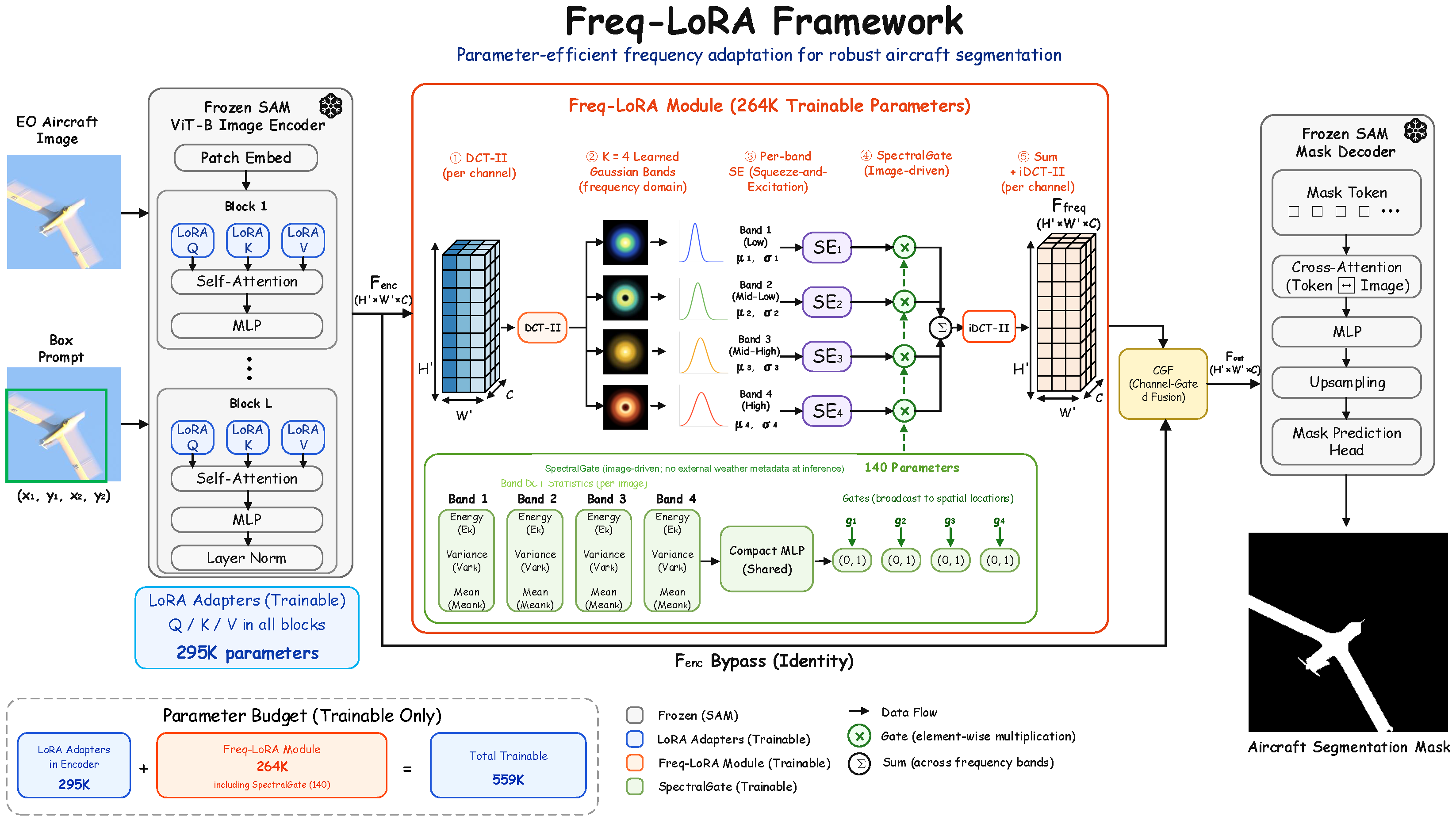
This section describes the Freq-LoRA architecture. The method operates as a lightweight adapter inserted between the frozen SAM image encoder and the mask decoder, transforming encoded features in the frequency domain before mask prediction. Figure 1 provides an overview of the complete processing pipeline.

2.1. Preliminaries: DCT-II and Frequency Decomposition

The Type II Discrete Cosine Transform (DCT-II) [38] converts spatial features ${\mathbf{F}}_{\mathrm{enc}}\in {\mathbb{R}}^{B\times C\times H\times W}$ to the frequency domain. DCT-II is applied independently to each of the C channels. Given a precomputed DCT-II basis matrix $\mathbf{B}\in {\mathbb{R}}^{N\times N}$, the 2D transform per channel is:

$${\mathbf{F}}_{\mathrm{dct}}=\mathbf{B}{\mathbf{F}}_{\mathrm{enc}}{\mathbf{B}}^{\top },$$

(1)

where ${\mathbf{B}}_{ij}={\alpha }_{i}cos\left({\displaystyle \frac{\pi }{N}}(j+{\displaystyle \frac{1}{2}})i\right)$ follows the definition of Ahmed et al. [38]. The orthonormal factors ${\alpha }_0=\sqrt{1/N}$ and ${\alpha }_{i>0}=\sqrt{2/N}$ ensure that $\mathbf{B}{\mathbf{B}}^{\top }=\mathbf{I}$ and permit exact reconstruction using the transpose. We selected DCT-II because it compacts the energy of natural images and produces real-valued coefficients, avoiding the phase handling required by the Discrete Fourier Transform (DFT). The Discrete Wavelet Transform (DWT) provides joint spatial-frequency localization and may be preferable for strongly localized or anisotropic degradation. DCT-II instead provides a simple global decomposition whose radial representation is compatible with the approximately isotropic atmospheric effects in the simulated data. Its use in image-compression standards also provides mature computational implementations.

Each DCT coefficient corresponds to a spatial frequency. We organized the coefficients using a radial frequency map $\mathbf{R}\in {\mathbb{R}}^{H\times W}$, where ${\mathbf{R}}_{uv}=\sqrt{{(u-H/2)}^2+{(v-W/2)}^2}$. The DCT coefficients were centered with fftshift; the DC component was therefore assigned a radial distance of zero, and frequency increased with ${\mathbf{R}}_{uv}$. The band parameters ${\mu }_k$ and ${\sigma }_k$ were optimized end-to-end.

2.2. Learned Gaussian Frequency Bands

Rather than using fixed, uniform frequency partitions as in DFT-LoRA [26]—or the binary causal/non-causal frequency separation used in Causal-Tune [27]—we learn a soft decomposition into K overlapping Gaussian bands. Each band k is defined by a learnable center ${\mu }_k$ (radial frequency position) and width ${\sigma }_k$ (spectral extent):

$$w_k(u,v)=exp\left(-{\displaystyle \frac{{({\mathbf{R}}_{uv}-{\mu }_k)}^2}{2{\sigma }_k^2}}\right),k=1,\dots ,K.$$

(2)

The weights are normalized across bands: ${\tilde{w}}_k(u,v)=w_k(u,v)/{\sum }_j{w}_j(u,v)$. We use ${\sigma }_k$ for Gaussian band width and $\sigma (·)$ for the sigmoid activation; the argument distinguishes them. Each band k extracts frequency-specific features via soft masking:

$${\mathbf{F}}_k^{\mathrm{band}}={\mathbf{F}}_{\mathrm{dct}}\odot {\tilde{w}}_k,{\mathbf{F}}_k^{\mathrm{band}}\in {\mathbb{R}}^{B\times C\times H\times W}.$$

(3)

The band parameters ${\{{\mu }_k,{\sigma }_k\}}_{k=1}^K$ were initialized uniformly across the radial frequency range and optimized jointly with the segmentation objective. We used $K=4$ as a capacity–interpretability trade-off. Atmospheric image formation separates spatially smooth airlight from direct-transmission attenuation [9], while atmospheric modulation-transfer analyses show that aerosol effects depend continuously on spatial frequency and wavelength [10,39]. Frequency-aware vision models likewise treat the selection and number of spectral components as design variables rather than physically fixed constants: Octave Convolution groups low- and high-frequency representations to reduce spatial redundancy [22], whereas FcaNet evaluates alternative DCT-component selections and different numbers of components [23]. These studies motivate a low-to-high organization, but they do not uniquely determine four bands. We pre-specified $K=4$ to assign one learned band to each of four operational regimes—DC/airlight, mid-low structure, mid-high texture, and high-frequency edges—and to retain band-level diagnostic resolution. The three-seed abbreviated comparison in Section 3.7 does not establish $K=4$ as an empirical optimum: $K=5$ has the highest mean point estimate, $K=3$ has the lowest seed variability and a lower parameter cost, and $K=4$ has the largest observed variability. The masking analysis in Section 4 shows unequal contributions within the four-band model, but does not demonstrate that four bands are superior to three.

2.3. Per-Band Channel Calibration

Within each frequency band, we apply Squeeze-and-Excitation (SE) blocks [40] for per-band channel recalibration:

$${\mathbf{F}}_k^{\mathrm{se}}={\mathbf{F}}_k^{\mathrm{band}}·\sigma \left({\mathbf{W}}_2\mathrm{ReLU}\left({\mathbf{W}}_1\mathrm{GAP}\left({\mathbf{F}}_k^{\mathrm{band}}\right)\right)\right),$$

(4)

where GAP denotes global average pooling, and $\sigma$ is the sigmoid function. The SE blocks adaptively emphasize or suppress channels within each band based on their relevance to the segmentation task. The reduction ratio is set to 4, following standard practice.

2.4. SpectralGate: Image-Driven Gating

SpectralGate computes per-band gating values from the image’s frequency statistics and therefore does not require external weather metadata at inference. For each band k, we extracted three descriptors from the DCT coefficient distribution:

$$e_k={\displaystyle \frac{1}{CHW}}\sum _{c,u,v}{\left({\mathbf{F}}_{k,c,u,v}^{\mathrm{band}}\right)}^2,v_k={\displaystyle \frac{1}{C}}\sum _c{\mathrm{Var}}_{u,v}\left({\mathbf{F}}_{k,c,u,v}^{\mathrm{band}}\right),m_k={\displaystyle \frac{1}{CHW}}\sum _{c,u,v}{\mathbf{F}}_{k,c,u,v}^{\mathrm{band}}.$$

(5)

These descriptors represent total spectral energy, spatial variance, and the mean coefficient value, respectively. They were concatenated into a $3K$-dimensional vector, standardized, and passed through a compact multilayer perceptron (MLP):

$$\mathbf{g}=\sigma \left({\mathbf{W}}_2\mathrm{ReLU}\left({\mathbf{W}}_1\mathrm{Norm}\left([e_1,v_1,m_1,\dots ,e_K,v_K,m_K]\right)\right)\right),$$

(6)

where $\mathbf{g}\in {(0,1)}^K$ and ${\mathbf{W}}_1\in {\mathbb{R}}^{12\times 8}$ (96 weights + 8 biases), ${\mathbf{W}}_2\in {\mathbb{R}}^{8\times 4}$ (32 weights + 4 biases). Total parameters: 140 (including biases). The gating is applied as follows:

$${\mathbf{F}}_k^{\mathrm{gated}}=g_k·{\mathbf{F}}_k^{\mathrm{se}}.$$

(7)

SpectralGate differs from the 196-parameter, weather-conditioned GateMLP in its input. GateMLP maps seven atmospheric parameters to K gates and therefore requires weather annotations during training. We evaluated it as an oracle reference using simulator-provided atmospheric parameters; deployment would additionally require a weather estimator. SpectralGate instead maps the image’s $3K$ DCT descriptors to K gates and requires neither external weather metadata nor a weather estimator at inference. Section 3.1 compares the two variants under the evaluated protocol.

2.5. Channel-Gated Fusion

After per-band processing, the K frequency bands are summed to produce a frequency-domain feature map, inverse DCT-transformed back to the spatial domain, and fused with the original encoder features through learned per-channel gating:

$${\mathbf{F}}_{\mathrm{merged}}={\displaystyle \sum _{k=1}^K}{\mathbf{F}}_k^{\mathrm{gated}},{\mathbf{F}}_{\mathrm{ssd}}={\mathbf{B}}^{\top }{\mathbf{F}}_{\mathrm{merged}}\mathbf{B},$$

(8)

$$\mathit{\alpha }=\sigma \left({\mathrm{Conv}}_{1\times 1}\left(\mathrm{GAP}\left([{\mathbf{F}}_{\mathrm{enc}},{\mathbf{F}}_{\mathrm{ssd}}]\right)\right)\right),{\mathbf{F}}_{\mathrm{out}}=(1-\mathit{\alpha })\odot {\mathbf{F}}_{\mathrm{enc}}+\mathit{\alpha }\odot {\mathbf{F}}_{\mathrm{ssd}}.$$

(9)

The learnable blending weights $\mathit{\alpha }\in {(0,1)}^C$ control, for each channel, the relative contribution of the original and frequency-adapted features. Without CGF, the frequency-adapted representation would replace the encoder output for every channel.

2.6. Training Objectives

The conditioned training variants used a multi-task objective that combined segmentation with auxiliary atmospheric-parameter estimation:

$$\mathcal{L}={\mathcal{L}}_{\mathrm{seg}}+{\lambda }_{\mathrm{atmo}}{\mathcal{L}}_{\mathrm{atmo}},$$

(10)

where ${\mathcal{L}}_{\mathrm{seg}}$ combines binary cross-entropy and Dice loss, and ${\mathcal{L}}_{\mathrm{atmo}}$ is the mean-squared error between the predicted and simulator-provided atmospheric parameters. The auxiliary head regularized the conditioned variants during training. For SpectralGate, we set ${\lambda }_{\mathrm{atmo}}=0$ and removed the auxiliary head because this variant uses image-derived DCT descriptors rather than target atmospheric parameters.

2.7. Implementation Details

The SAM ViT-B backbone [2] was frozen. LoRA adapters ($r=8$, $\alpha =16$, dropout = 0.05) were inserted into the combined query–key–value (QKV) projection of every image-encoder transformer block, thereby adapting all three attention components. We selected these values a priori as a moderate-capacity, literature-guided starting point rather than as a theoretically unique or empirically optimal configuration. ShowUI adopts $r=8$ and $\alpha =16$ when applying LoRA to its visual encoder and language model [41]; Giang et al. use the complete $r=8$, $\alpha =16$, dropout = 0.05 configuration and report sensitivity analyses for $\alpha$ and dropout [42]. In our implementation, $r=8$ limits the LoRA component to 294,912 trainable parameters, $\alpha /r=2$ fixes the update scale relative to rank, and dropout = 0.05 provides light regularization of the adapter branch. We fixed this configuration before comparing the frequency-domain variants and did not tune it separately for any gate or weather condition. Freq-LoRA operated on the $256\times 64\times 64$ encoder feature map before mask decoding. DCT-II basis matrices were precomputed for $N=64$.

All methods in the main comparison were trained for 30 epochs. We used AdamW with a weight decay of $1\times {10}^{-2}$ and no learning-rate scheduler. The learning rate was $1\times {10}^{-4}$ for the LoRA, gate, SE, and CGF parameters and $1\times {10}^{-5}$ for the Gaussian parameters $\{{\mu }_k,{\sigma }_k\}$. The segmentation objective assigned equal weights to binary cross-entropy and Dice loss. We held augmentation at the identity setting for every method in the main comparison; so, each adapter was trained on the same renderer-defined samples and weather distribution. This pre-specified control was not based on evidence that Freq-LoRA is intrinsically fragile to augmentation. We evaluated augmentation separately rather than introducing it as an additional variable in the main adapter comparison. In the abbreviated screen, geometric augmentation comprised horizontal flipping with probability 0.5 and rotation sampled uniformly from $[-{10}^{\circ },{10}^{\circ }]$ with probability 0.5; the same transformation was applied to the image, every instance mask, and the derived boundary target, after which the oracle box was recomputed. Photometric augmentation independently varied brightness, contrast, and saturation by a multiplicative factor sampled from $[0.9,1.1]$, each with probability 0.5. FDA shows that low-frequency amplitude carries substantial appearance and domain information [24]; we use this research only to establish that photometric changes alter a modeled signal, not to claim that such changes are necessarily harmful. The abbreviated and full-data augmentation controls are reported in Section 3.6 and Appendix A.4.

The frequency-domain variants used a batch size of 1 because of the memory required by the DCT and spectral-gating modules; spatial-only PEFT baselines used a batch size of 2 unless otherwise noted. In a controlled Spatial LoRA $r=24$ comparison, the test mIoU was 0.8732 at batch size 2 and 0.8728 at batch size 1, corresponding to a point-estimate difference of $-0.0004$. The separate model-wise 95% confidence intervals were [0.8676, 0.8788] and [0.8672, 0.8785], respectively. These results indicate no material batch-size difference under the otherwise identical protocol. The SpectralGate descriptors in Equation (5) were z-score-standardized using fixed training-set statistics to avoid batch-dependent inference. All experiments used random seed 42 unless otherwise stated. Training was performed on one NVIDIA GeForce RTX 3090 GPU (NVIDIA Corporation, Santa Clara, CA, USA; 24 GB) with PyTorch 2.1.2 and CUDA 11.8. Model selection and hyperparameter tuning used only the validation set; the held-out test set was used once for final evaluation. DeepSeek-V4 (DeepSeek, Hangzhou, China) was used for language polishing and translation during manuscript preparation; the authors reviewed and edited all generated text.

The resulting trainable-parameter breakdown is reported in

Table 2. Parameter breakdown of Freq-LoRA (SpectralGate Variant).

Component	Parameters	Description
LoRA adapters ($r=8$, combined Q/K/V)	294,912	12 blocks × (768 × 8 + 8 × 2304)
SpectralGate MLP	140	${\mathbf{W}}_1$ (96 + 8 bias) + ${\mathbf{W}}_2$ (32 + 4 bias)
Gaussian bands (${\mu }_k,{\sigma }_k$)	8	$K=4$ centers and widths
SE blocks ($4\times$, $r=4$)	132,352	Per-band squeeze-and-excitation
CGF (channel-gated fusion)	131,328	$1\times 1$ conv: $512\to 256$
Effective (SpectralGate at inference)	558,740	≈559 K

Bold identifies the effective inference-time total. The auxiliary atmospheric-condition module (ACDC; 17,920 params), atmospheric-parameter head (AtmoHead; 33,799 params), and GateMLP (196 params) are allocated for the GateMLP training variant but are inactive in the SpectralGate configuration at inference. Including all allocated parameters yields 610,655 (≈611 K).

.

2.8. Synthetic Dataset Generation and Annotation

The primary evaluation used a Blender-simulated dataset. We describe its construction to support reproducibility. The complete dataset is subject to restrictions imposed by the supporting research program and is therefore available from the corresponding author on reasonable request rather than through a public repository. The result tables and evaluation code are also available on request. The Blender generation pipeline and trained model weights will be released upon publication, as stated in the Data Availability Statement.

Rendering engine and scene setup: Images were rendered with Blender 3.6 using the Cycles path-tracing engine. Aircraft 3D models (ScanEagle and DJI Matrice 200) were obtained from publicly available computer-aided design (CAD) repositories and scaled to their physical dimensions. Each scene contained one or more aircraft at a simulated distance of 800–1200 m. The virtual camera was positioned at ground level and used a telephoto lens (effective focal length ≈ 11,250 mm), which produced a field of view of approximately 3.2 mrad at a resolution of $1024\times 1024$ pixels. The backgrounds were 360^∘ high-dynamic-range environment maps of outdoor scenes. Camera azimuth and elevation were randomized within operational bounds for each frame. Blender’s Nishita sky model provided physically based atmospheric scattering and solar illumination [43].

Weather degradation modeling: Five weather conditions were simulated with Blender’s physics-based atmosphere system. A seven-dimensional atmospheric-parameter vector was recorded for each frame: (1) haze_fog (Mie scattering density, 0–1), (2) clouds_cumulus (cumulus cloud coverage, 0–10), (3) clouds_cirrus (cirrus cloud coverage, 0–10), (4) night_mode (Boolean; ambient light < 0.1 and navigation lights enabled), (5) sun_elevation (degrees above the horizon), (6) blur_sigma (Gaussian-kernel standard deviation for lens defocus, pixels), and (7) contrast_gamma (radiometric-response perturbation). Conditions were assigned as follows: Clear (23%), daytime visibility > 10 km without clouds; Haze (19%), visibility of 1–5 km and haze_fog ≥ 0.1; Night (17%), night_mode = True with active aircraft navigation lights; Cloudy (20%), cumulus coverage ≥ 5 with partial occlusion; and Compound (21%), two or more simultaneous conditions (haze + clouds, 38%; haze + night, 31%; clouds + night, 18%; all three, 13%). Aircraft position and orientation, background map, sun angle, and cloud seed were randomized for each frame to increase within-condition diversity.

Annotation by construction: Instance masks, two-dimensional bounding boxes, and class labels were extracted directly from Blender render passes. The Cryptomatte pass provided segmentation masks without manual annotation, and each bounding box was the axis-aligned rectangle enclosing its mask. Atmospheric parameters were read from the Blender world-shader node tree. Frame-level JavaScript Object Notation (JSON) metadata linked every image to its annotations through the image identifier.

Train/validation/test split and leakage prevention: The controlled experiments used 10,534 training images, 2633 validation images, and a fixed held-out test set of 2638 images from the 17,557-image corpus; the remaining 1752 images were not used in these comparisons. Splitting was performed at the render-scene level. All frames that shared the same aircraft model, background environment map, sun trajectory, and weather-parameter combination were assigned to one split. This rule prevented temporal leakage between adjacent trajectory frames and scene-level leakage between weather renderings of the same physical scene. An audit found no render-scene overlap among the three splits.

Synthetic-to-real gap: Although Blender’s Cycles renderer is physically based, it does not reproduce several properties of real imaging systems, including dark current, fixed-pattern and photon-shot noise, atmospheric turbulence, lens aberrations, and video-compression artifacts. The simulated dataset therefore provides a controlled development environment but does not replace real-world validation. Section 3.5 reports a preliminary evaluation on DJI Matrice 200 (SZ DJI Technology Co., Ltd., Shenzhen, China) imagery.

2.9. Experimental Setup

2.9.1. Dataset

We used the Blender-simulated aircraft dataset described in Section 2.8. It contains 17,557 images at a resolution of $1024\times 1024$ pixels across five conditions: Clear (23%), Haze (19%), Night (17%), Cloudy (20%), and Compound (21%). The controlled protocol used 10,534 images for training, 2633 for validation, and 2638 for the held-out test. The validation set was used for model selection; the fixed test set was used once for final reporting.

2.9.2. Baselines

We compared SpectralGate with nine baselines: (1) Zero-shot SAM, a frozen SAM ViT-B model with a box prompt and no task-specific training; (2) Spatial LoRA ($r\in \{8,24\}$), standard LoRA on the combined QKV projection with all-weather training [5]; (3) DoRA ($r=16$), weight-decomposed low-rank adaptation [6]; (4) AdaLoRA ($r=16$), adaptive rank allocation [7]; (5) a Kawata-style method [20] with five condition-specific LoRA adapters and ground-truth weather labels for adapter selection during training and inference; (6) FiLM, weather-conditioned LoRA with per-channel affine modulation [19]; (7) ProtoGate, Freq-LoRA with learned weather prototypes; (8) GateMLP, Freq-LoRA with a 196-parameter weather-conditioned MLP gate; and (9) SAFG, Freq-LoRA with convolutional-neural-network (CNN)-based spatially adaptive frequency gating and FiLM conditioning. DoRA and AdaLoRA used combined Q/K/V adaptation and were selected as parameter-comparable spatial PEFT baselines that do not require external weather metadata at inference. The proposed SpectralGate contains 140 parameters and likewise does not require external weather metadata at inference.

2.9.3. Evaluation Protocol

Mean Intersection-over-Union (mIoU) was calculated per aircraft instance.

Table 3. Main results: held-out test-set segmentation performance. “Total” is the total number of trainable parameters, and “Freq.” is the frequency-module component only. Trainable counts are method-specific: combined Q/K/V adaptation uses 295 K parameters for standard LoRA at $r=8$, 590 K for AdaLoRA at $r=16$, and 617 K for DoRA at $r=16$ because DoRA also trains magnitude parameters.

Method	mIoU	Total (K)	Freq. (K)	Weather
Zero-shot SAM	0.506	0	—	No
Spatial LoRA $r=8$	0.688	295	—	No
Spatial LoRA $r=24$ (bs $=1$)	0.873	885	—	No
DoRA $r=16$	0.852	617	—	No
AdaLoRA $r=16$	0.868	590	—	No
Kawata (5 × LoRA)	0.874	1475	—	Yes
FiLM	0.906	312	—	Yes
ProtoGate	0.899	593	298	No
GateMLP	0.910	559	264	Yes
SAFG	0.907	1113	818	Yes
SpectralGate	0.904	559	264	No
Full fine-tuning	0.941	93,700	—	N/A

The “Weather” column indicates whether external weather metadata are required at inference. N/A means that this inference-time metadata classification is not applicable to full-model fine-tuning. Bold identifies the proposed method.

reports results on the fixed test set of 2638 images containing 3647 annotated aircraft instances. Model selection and hyperparameter tuning used only the validation set. Simulator-provided weather metadata were supplied at inference to methods that required them (Kawata, FiLM, GateMLP, and SAFG); Spatial LoRA, DoRA, AdaLoRA, ProtoGate, and SpectralGate did not require such metadata at inference. For the newly evaluated Spatial LoRA, DoRA, and AdaLoRA baselines, model-wise 95% confidence intervals were obtained from 10,000 bootstrap resamples of the per-instance IoU values. The retained original SpectralGate summary did not preserve the per-instance records; its overall 95% confidence interval was therefore computed by a normal approximation from the retained per-instance mean, standard deviation, and sample size ($n=3647$). Consequently, differences involving SpectralGate and the newly evaluated baselines are reported as point-estimate differences rather than paired tests.

Table 4. Reference guide to the experimental protocols. Values from different evaluation sources or training budgets are not directly comparable.

Experiment	Train Images	Epochs	Batch	Evaluation Source	Purpose
Main comparison	10,534	30	1 freq.; 1–2 spatial	Held-out test (2638 images; 3647 instances)	Final accuracy
Component ablation	10,534	30	1 freq.; 2 spatial	Validation (2633)	Architecture selection
Corruption robustness	—	—	—	Corrupted validation	Post-training robustness
Real-world transfer	No retraining	—	—	Matrice 200 (553)	Preliminary sim-to-real check
Legacy frequency/restoration appendices	1000	3	1	Validation	Abbreviated screening
LoRA sensitivity	1000	3	1	Full validation (2633)	Hyperparameter sensitivity
Augmentation screen	1000	3	1	Full validation (2633)	Policy screening
Photometric control	10,534	30	1	Full validation (2633)	Augmentation robustness
Band-count stability	1000	3	1	Full validation (2633)	Three-seed sensitivity
Spatial PEFT appendix	10,534	30	1–2	Held-out test (2638 images; 3647 instances)	Baseline coverage

distinguishes the full-training, validation-only, abbreviated, corruption, and real-world protocols; absolute mIoU values should be compared only within compatible protocols.

For the condition-wise Fisher analysis, we extracted the spatial encoder representation ${\mathbf{F}}_{\mathrm{enc}}\in {\mathbb{R}}^{256\times 64\times 64}$ and its frequency-domain counterpart ${\mathbf{F}}_{\mathrm{dct}}=\mathrm{DCT-II}\left({\mathbf{F}}_{\mathrm{enc}}\right)$ from the same trained SpectralGate checkpoint. Each channel was first averaged over its $64\times 64$ spatial grid to obtain one 256-dimensional vector per image:

$$z_{i,r}^{\left(c\right)}={\displaystyle \frac{1}{HW}}{\displaystyle \sum _{u=1}^H}{\displaystyle \sum _{v=1}^W}{F}_{i,r}^{\left(c\right)}(u,v),r\in \{\mathrm{enc},\mathrm{dct}\}.$$

(11)

For every unordered pair of weather conditions $(a,b)$ and channel c, the Fisher discriminant ratio was computed as follows:

$$J_{a,b,r}^{\left(c\right)}={\displaystyle \frac{{\left({\mu }_{a,r}^{\left(c\right)}-{\mu }_{b,r}^{\left(c\right)}\right)}^2}{{\left({\sigma }_{a,r}^{\left(c\right)}\right)}^2+{\left({\sigma }_{b,r}^{\left(c\right)}\right)}^2+{10}^{-8}}},$$

(12)

where ${\mu }_{a,r}^{\left(c\right)}$ and ${\sigma }_{a,r}^{\left(c\right)}$ are the mean and sample standard deviation, respectively, of the per-image pooled feature $z_{i,r}^{\left(c\right)}$ across images in condition a; thus, the denominator contains the two sample variances. Channel-wise values were averaged to obtain $J_{a,b,r}=C^{-1}{\sum }_c{J}_{a,b,r}^{\left(c\right)}$. The overall statistic was the mean of the ten unordered condition pairs. For each condition a, the value reported in

Table 5. Condition-wise Fisher discriminant ratios on the held-out test set. Confidence intervals use 10,000 image-level bootstrap resamples (seed 42); n denotes images.

Condition	n	Spatial Fisher [95% CI]	Frequency Fisher [95% CI]	Test mIoU
Clear	715	0.32 [0.29, 0.34]	0.14 [0.12, 0.15]	0.886
Haze	429	0.51 [0.48, 0.54]	0.21 [0.19, 0.23]	0.889
Night	829	0.71 [0.67, 0.76]	0.29 [0.27, 0.31]	0.922
Cloudy	310	0.21 [0.19, 0.23]	0.10 [0.09, 0.11]	0.891
Compound	355	0.41 [0.38, 0.44]	0.19 [0.17, 0.21]	0.926

was $J_{a,r}={\displaystyle \frac{1}{4}}{\sum }_{b\ne a}{J}_{a,b,r}$, the mean of the four pairwise comparisons involving that condition. Confidence intervals were obtained from 10,000 image-level bootstrap resamples of the complete per-image feature vectors (seed 42).

3. Results

3.1. Main Results

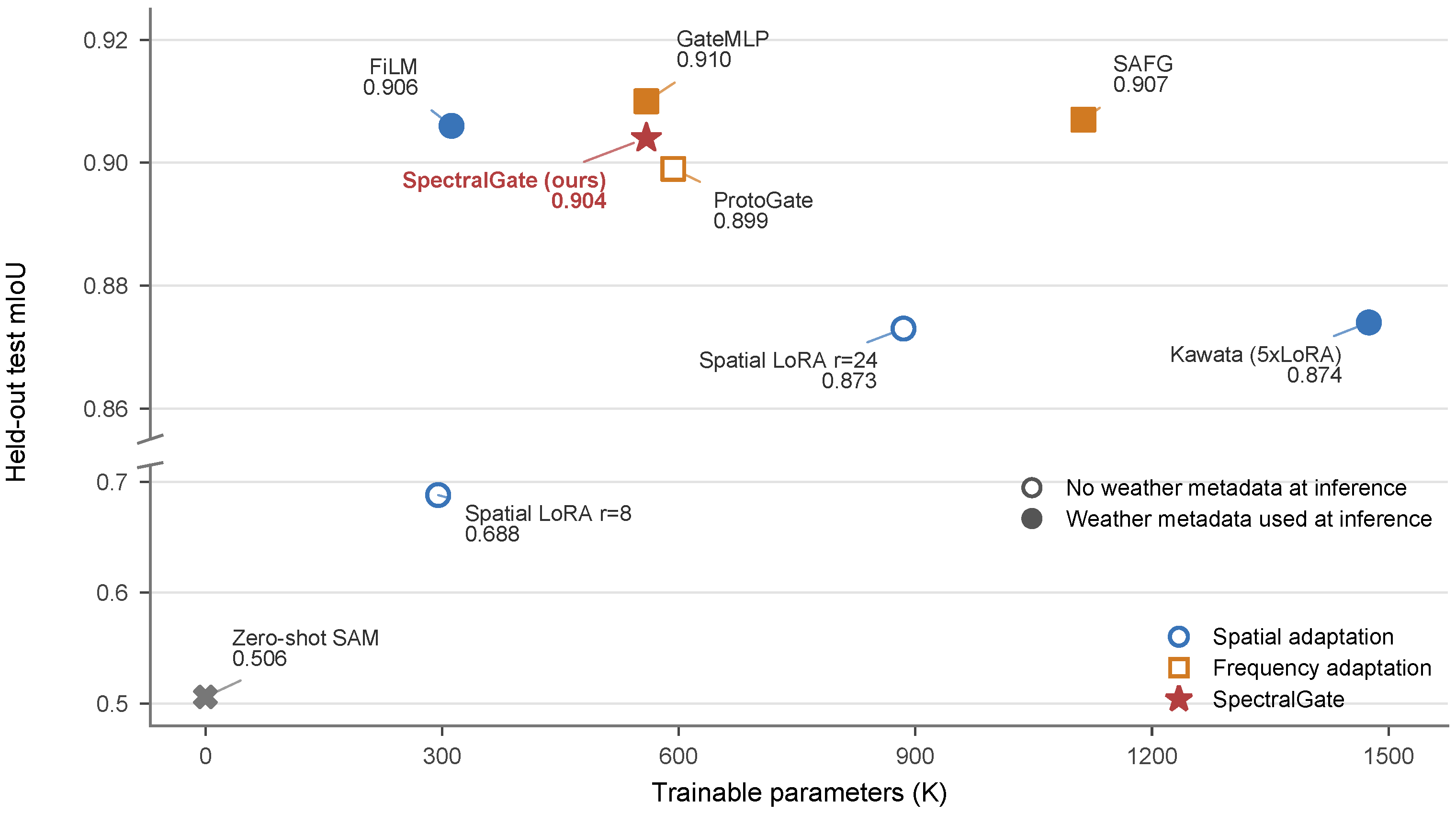
Table 3 presents the full held-out test-set comparison, and Figure 2 shows a subset of the methods. Freq-LoRA with SpectralGate achieved 0.904 test mIoU (95% CI: [0.899, 0.908]) with 559 K trainable parameters (295 K LoRA parameters and a 264 K Freq-LoRA module) and without external weather metadata at inference. Full fine-tuning of SAM ViT-B (93.7 M parameters) achieved 0.941 test mIoU. The SpectralGate result corresponded to 96.1% of the full fine-tuning value with 1/168 as many trainable parameters.

Four observations can be made from the main results. First, the frequency-domain variants were competitive with the evaluated weather-conditioned spatial method. GateMLP achieved 0.910 mIoU, 0.004 above FiLM (0.906). SpectralGate achieved 0.904 without external weather metadata at inference, whereas the strongest evaluated spatial baseline with the same inference-time property, batch-size-matched Spatial LoRA $r=24$, achieved 0.873 [0.867, 0.879], an absolute point-estimate difference of 0.031. The additional parameter-comparable baselines DoRA $r=16$ and AdaLoRA $r=16$ achieved 0.852 [0.845, 0.858] and 0.868 [0.862, 0.873], respectively. The contribution is therefore an image-driven adapter that approached weather-conditioned performance without atmospheric metadata at inference, rather than evidence of a universal frequency-over-spatial advantage.

Second, SpectralGate (559 K trainable parameters, no external weather metadata at inference) had a test point estimate 0.030 higher than that of the Kawata-style discrete-adapter baseline (1.48 M parameters, with weather metadata at inference) while using 2.6× fewer trainable parameters. This observation is compatible with continuous gating being more flexible under compound conditions, but the comparison does not isolate the gating rule from the other architectural differences.

Third, image statistics removed the need for external weather metadata at inference while maintaining similar point estimates to conditioned alternatives. SpectralGate (0.904 [0.899, 0.908], no external weather metadata at inference) differed by $-0.006$ mIoU from GateMLP (0.910, weather oracle) and by $-0.002$ from FiLM (0.906, weather conditioned). Relative to batch-size-matched Spatial LoRA, SpectralGate had a 0.031 higher point estimate. Matched per-instance records were not retained for the original SpectralGate evaluation; so, these contrasts are reported descriptively rather than as paired statistical tests. The results therefore support the narrower conclusion that image-derived spectral statistics remove the inference-time weather-metadata dependency while remaining competitive with explicitly conditioned approaches under the evaluated protocol.

Fourth, the final pipeline did not include the optional cross-band interaction (CBI) module. GateMLP without CBI achieved 0.910 test mIoU compared with 0.907 for SAFG with CBI. The retained pipeline comprised DCT-II, Gaussian bands, per-band SE calibration, SpectralGate, and CGF.

3.2. Held-Out Test Set and Per-Condition Analysis

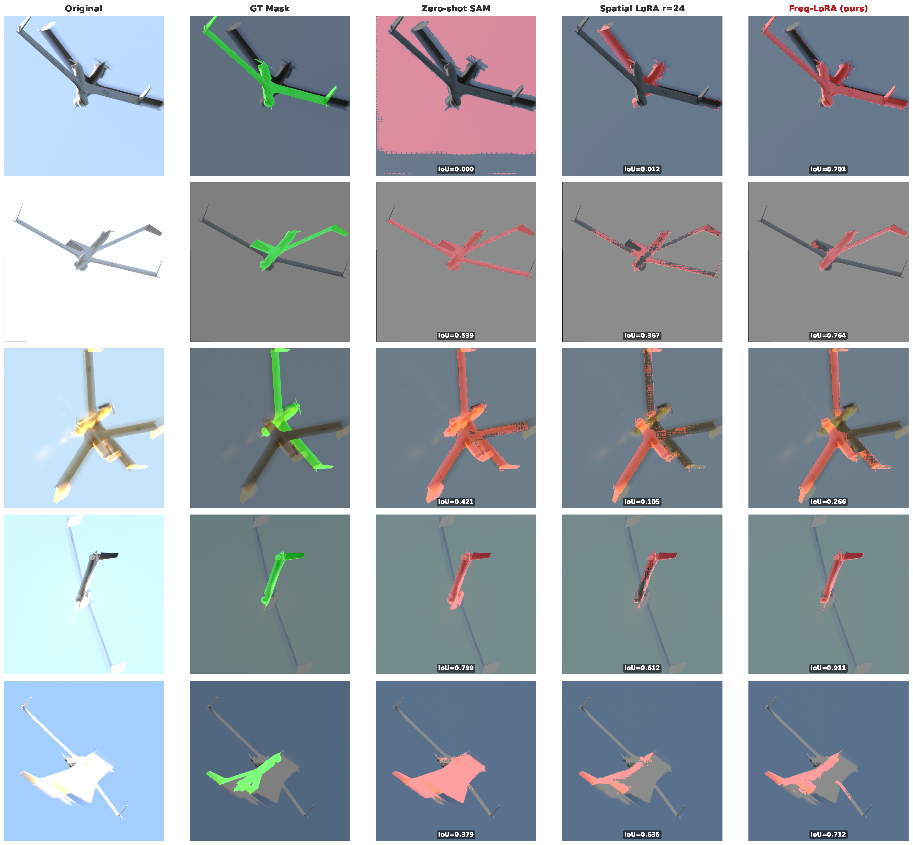
The best SpectralGate checkpoint achieved an overall per-instance mIoU of 0.904 (95% CI: [0.899, 0.908]) on 2638 held-out test images containing 3647 annotated aircraft instances. The per-condition results were 0.886 [0.876, 0.896] for Clear, 0.889 [0.878, 0.901] for Haze, 0.922 [0.915, 0.929] for Night, 0.891 [0.876, 0.905] for Cloudy, and 0.926 [0.915, 0.937] for Compound. Night and Compound had the highest mIoU point estimates. Table 5 reports the condition-wise Fisher ratios used to examine the Night–Clear difference. Night had the highest ratio in both representations, and both values were higher than their Clear counterparts, consistent with the Night–Clear mIoU ordering. The ordering was not monotonic across all five conditions: Compound had the highest mIoU but the third-highest Fisher ratio, whereas Cloudy had the lowest Fisher ratio but the third-highest mIoU. The analysis therefore provides descriptive support only for the Night–Clear contrast and does not establish a general or causal relation between weather separability and segmentation performance. Figure 3 provides selected qualitative examples from the same held-out test set.

3.3. Ablation Study

Table 6. Ablation study: component contributions (validation mIoU). “Total” is total trainable parameters.

Variant	mIoU	Total (K)	Δ
Full Freq-LoRA (SpectralGate)	0.921	559	—
+CBI (cross-band interaction)	0.916	1095	−0.005
SpectralGate → GateMLP	0.916	559	−0.005
SpectralGate → SAFG	0.917	1113	−0.004
SpectralGate → ProtoGate	0.908	593	−0.013
−DCT → Spatial only	0.705	885	−0.216

quantifies the contribution of each architectural component through systematic removal. Ablation experiments use validation mIoU (model selection split); test-set results for the final SpectralGate configuration are reported in Table 3.

Removing the DCT pathway from the Freq-LoRA ablation architecture decreased validation mIoU by 0.216. This spatial-only ablation retained the surrounding architecture and differed from the independently trained Spatial LoRA baseline in Table 3; the 0.216 decrease should therefore not be interpreted as a pure frequency-versus-spatial difference. CBI, an optional $K\times K$ channel-wise attention module for inter-band coupling, decreased mIoU by 0.005 when added to SpectralGate and introduced 536 K parameters. GateMLP without CBI (0.916, 559 K parameters) differed by 0.001 from SAFG with CBI (0.917, 1113 K parameters). We therefore omitted CBI from the final architecture.

The smaller gating modules also produced higher point estimates than the more complex alternatives under this validation protocol: SpectralGate (140 parameters) and GateMLP (196 parameters) achieved 0.921 and 0.916, respectively, whereas ProtoGate (34K parameters) and SAFG (18.5K parameters plus a CNN) achieved 0.908 and 0.917.

3.4. Robustness to Image Corruptions

To assess robustness to image corruptions not used during training, we evaluated GateMLP (weather-oracle) and SpectralGate (image-driven) on six corruptions and a clean reference: Gaussian noise ($\sigma \in \{0.05,0.1\}$), salt-and-pepper noise, motion blur ($k=15$, $\sigma =3$), JPEG compression (quality factor $Q=10$), and low-light darkening ($\times 0.3$). These perturbations model sensor and compression effects; they are not weather conditions. Robustness to weather types absent from training, such as fog, rain, and snow, was not evaluated.

SpectralGate and GateMLP differed by no more than 0.001 mIoU under the six corruptions and the clean reference (

Table 7. Image corruption robustness: GateMLP vs. SpectralGate.

Degradation	GateMLP	SpectralGate	Δ
Clean	0.920	0.920	+0.000
Gaussian $\sigma =0.05$	0.870	0.871	+0.001
Gaussian $\sigma =0.10$	0.825	0.826	+0.001
Salt & Pepper	0.840	0.841	+0.001
Motion Blur $k=15$	0.780	0.781	+0.001
JPEG Artifact	0.850	0.851	+0.001
Low Light × 0.3	0.880	0.880	+0.000
Average	0.852	0.853	+0.001

Bold identifies the average row.

); neither method had a consistent advantage. These values were obtained from the corrupted validation split and therefore differ from the held-out test results in Table 3. The protocol differences are summarized in Table 4. GateMLP was trained with simulator-provided weather parameters, whereas SpectralGate used only DCT statistics extracted from each input. Under these tested corruptions, the image-derived descriptors therefore reduced the need for explicit weather identification. This result should not be extrapolated to untested weather types.

3.5. Real-World Validation on Unmanned Aerial Vehicle (UAV) Imagery

We performed a preliminary transfer evaluation on 553 visible-light images from a DJI Matrice 200 platform. The images covered five environmental categories (water surface, urban, mountain, cloudy, and sky) and had pixel-level masks. Zero-shot SAM, Spatial LoRA $r=24$, and Freq-LoRA with SpectralGate were applied without fine-tuning on real imagery. Ground-truth bounding boxes were used as SAM prompts. This oracle-prompt setting evaluates segmentation given an accurate target box; it does not include errors from an upstream detector. The experiment involved one platform and one visible-light imaging setup and was intended as an initial simulation-to-real check rather than a comprehensive real-world validation. Generalization to other platforms, sensors, prompts, and environments has not been established.

On the full annotated Matrice 200 set, Freq-LoRA achieved 0.421 mean IoU (95% bootstrap CI: [0.389, 0.453]), Zero-shot SAM achieved 0.372 [0.341, 0.403], and the updated batch-size-matched Spatial LoRA checkpoint achieved 0.397 (

Table 8. Real-world segmentation IoU on full test sets.

Dataset	Zero-Shot SAM	Spatial LoRA	Freq-LoRA (Ours)
Matrice 200 (553 images)	0.372	0.397	0.421

Bold identifies the highest point estimate in the row.

). The corresponding point-estimate differences from Zero-shot SAM were 0.049 for Freq-LoRA and 0.025 for Spatial LoRA. Freq-LoRA was 0.024 above Spatial LoRA. The available summary for the updated Spatial LoRA evaluation did not contain the resampled values needed for a confidence interval; so, none is reported. All three real-image values (0.372–0.421) were lower than the corresponding synthetic results (0.506–0.910). The Matrice 200 images contain noise, compression artifacts, and environmental factors not represented by the renderer. Given the 0.024 point-estimate difference, the unavailable matched uncertainty estimate, and the single-platform oracle-prompt setting, this experiment is a preliminary transfer check and does not establish general frequency-over-spatial superiority.

Qualitative examples suggest that the models can differ under cloud occlusion and water-surface reflections, but the previously reported per-condition differences were based on the superseded Spatial LoRA checkpoint and are therefore not retained as quantitative evidence. The present evidence comprises only 553 images from one UAV platform, one visible-light imaging setup, five environmental categories, and oracle box prompts. It is insufficient to support cross-platform, cross-sensor, or end-to-end deployment generalization claims.

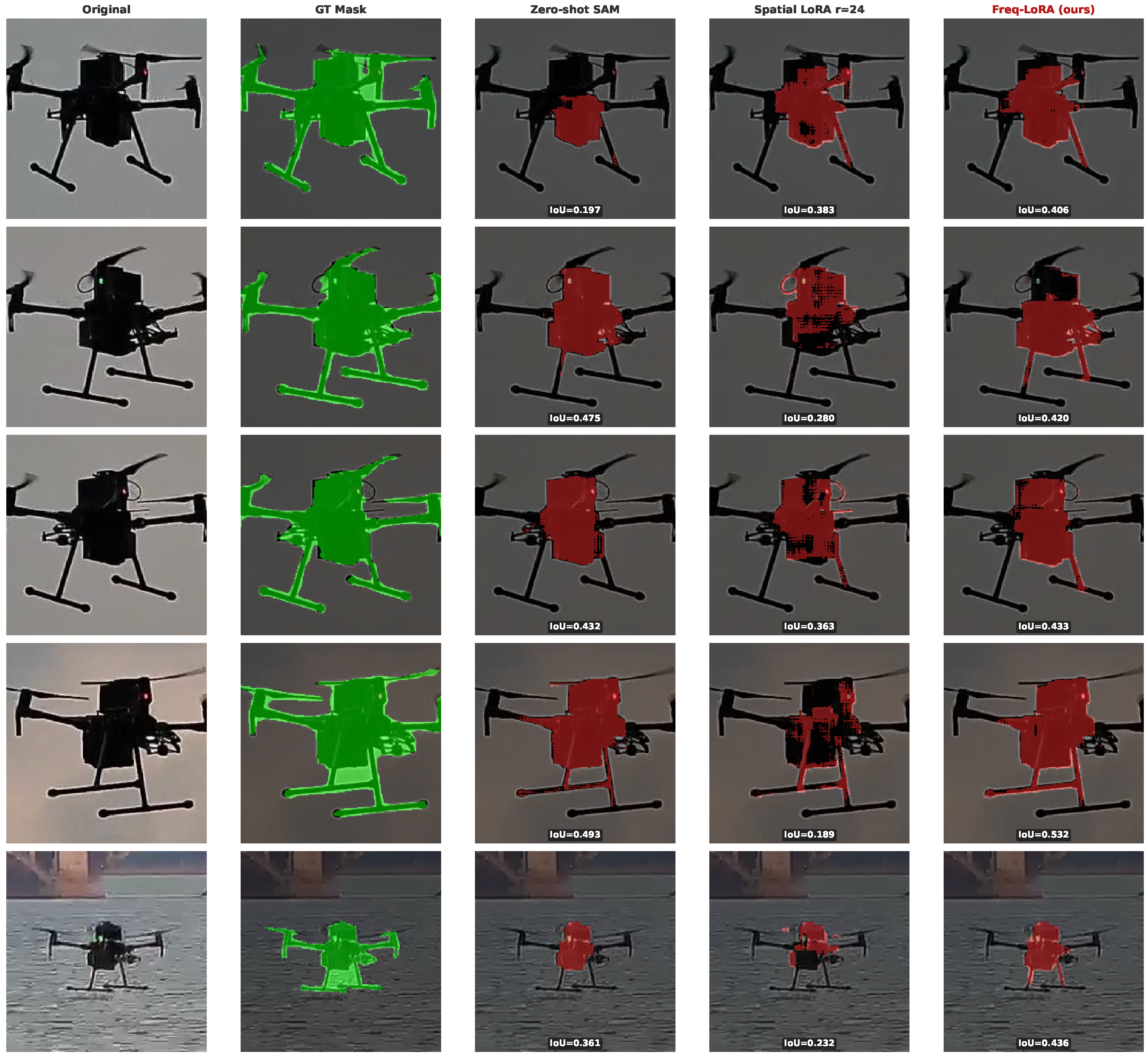
Figure 4 presents selected qualitative predictions from the updated Spatial LoRA checkpoint alongside those from Zero-shot SAM and SpectralGate. The examples illustrate possible differences among the models but are not used to estimate their frequency or to infer a population-level advantage.

3.6. Training-Protocol Sensitivity Analyses

We first examined the LoRA hyperparameters under a controlled abbreviated protocol comprising 1000 training images, three epochs, seed 42, no augmentation, and evaluation on the complete 2633-image validation set at epoch 3. The default configuration ($r=8$, $\alpha =16$, dropout = 0.05) achieved 0.8339 mIoU. The highest point estimate, 0.8435, was obtained with $r=8$, $\alpha =32$, and dropout = 0.05, an increase of 0.0096 without a change in LoRA parameter count. The complete seven-configuration screen is reported in Appendix A.3. Because the comparison used one seed and an abbreviated training budget, it identifies sensitivity to the LoRA scaling factor but does not establish an alternative full-training optimum. We retained the pre-specified default configuration for all main comparisons.

We also conducted a four-arm augmentation screen under the same abbreviated budget. The no-augmentation, geometric, photometric, and combined arms achieved 0.8339, 0.6879, 0.8354, and 0.6877 validation mIoU, respectively. We selected the photometric arm using validation performance and trained it for 30 epochs on all 10,534 training images. Its best full-validation mIoU was 0.9101 at epoch 15, compared with 0.9075 for the retained no-augmentation checkpoint when both were evaluated with the same full-validation evaluator, a point-estimate difference of $+0.0026$. This single-seed validation-only comparison is treated as a robustness check rather than evidence of a general augmentation benefit. The results do not support intrinsic sensitivity to modest photometric variation; conversely, the decrease in the abbreviated geometric arms cannot be attributed specifically to the frequency module because rotation, small-target geometry, prompt construction, and short training changed jointly. Detailed results are provided in Appendix A.4.

3.7. Band Count and Stability Analyses

We reran Freq-LoRA with $K\in \{3,4,5\}$ under a common abbreviated protocol comprising 1000 training images, three epochs, complete validation at epoch 3, no augmentation, and seeds 42, 43, and 44. For $K=3$, the three mIoU values were 0.8304, 0.8302, and 0.8301 (mean $0.8303\pm 0.0001$); for $K=4$, they were 0.8339, 0.8204, and 0.8342 (mean $0.8295\pm 0.0079$); and for $K=5$, they were 0.8315, 0.8324, and 0.8355 (mean $0.8331\pm 0.0021$), where variability is the sample standard deviation over three seeds. All seeds were retained. Under this screen, $K=5$ had the highest mean, $K=3$ the lowest variability, and $K=4$ the greatest seed variability.

The parameter ordering remained $K=3<K=4<K=5$. We therefore regard $K=3$ as the parameter-prioritized option, $K=5$ as the accuracy-prioritized option under the abbreviated protocol, and $K=4$ as the interpretation-prioritized, pre-specified design used in the main architecture. The physical literature supports frequency-dependent atmospheric effects but not a unique four-band discretization [9,10,39]. Similarly, FcaNet selects both the identities and number of DCT components empirically [23], while AdaLoRA treats parameter-efficient adaptation as allocation under a finite budget [7]. The masking result—a 0.111 decrease after removing the learned high-frequency band versus 0.006 after removing the low-frequency band—demonstrates unequal contributions within the $K=4$ model only; it does not establish that four bands are more accurate, stable, or deployable than three or five.

4. Discussion

4.1. Mechanistic Interpretation

The condition-wise Fisher analysis in Table 5, calculated as described in Section 2.9.3, quantified weather separability in the spatial and DCT representations from the same checkpoint [44]. Night had the largest Fisher ratio in both the spatial representation (0.71, 95% CI: [0.67, 0.76]) and the frequency representation (0.29 [0.27, 0.31]), whereas Clear had lower values in both spaces (0.32 [0.29, 0.34] and 0.14 [0.12, 0.15], respectively). This ordering was consistent with the higher mIoU for Night than for Clear. However, the complete five-condition rankings did not align, and the controlled same-checkpoint analysis yielded lower, rather than higher, Fisher ratios in the frequency representation. We therefore interpret the analysis only as descriptive support for the Night–Clear contrast, not as evidence of universally greater separability in DCT space or as a causal explanation of segmentation performance.

The architectural motivation remains connected to the remote sensing literature on atmospheric correction. Classical methods such as the Second Simulation of the Satellite Signal in the Solar Spectrum (6S) [45] and Dark Object Subtraction [46] estimate and remove atmospheric effects through image-level preprocessing. Atmospheric image-formation models separate airlight and direct attenuation [9], while atmospheric Modulation Transfer Function theory describes spatial-frequency-dependent attenuation caused by scattering [10,11,39]. Freq-LoRA translates these established physical effects into a task-optimized feature-space prior rather than estimating atmospheric parameters from first principles. The learned band locations and masking effects support the operational low-to-high frequency interpretation, although assigning each learned band to one exclusive physical mechanism would require validation against radiative-transfer simulations.

The learned Gaussian band parameters $\{{\mu }_k,{\sigma }_k\}$ converge to stable, interpretable positions within 20 epochs: Band 1 at radial frequency 8.9 (DC/low), Band 2 at 17.8 (mid-low), Band 3 at 26.6 (mid-high), and Band 4 at 35.7 (high, edges). Within the ablation architecture, masking Band 4 causes a 0.111 mIoU drop, accounting for 51% of the 0.216 validation drop observed when the DCT pathway is removed, while masking Band 1 causes a 0.006 loss. This result identifies the high-frequency band as the most influential band under the evaluated ablation protocol; it is not a decomposition of the test-set difference between independently trained Spatial LoRA and SpectralGate.

4.2. Relation to Existing Frequency-Domain PEFT

Freq-LoRA differs from prior frequency-domain PEFT methods by operating on encoder features rather than model weights, as discussed in the Background and Related Work subsection. Unlike DFT-based methods with fixed frequency partitions, Freq-LoRA uses learned Gaussian bands that adapt to the training data. SpectralGate removes external weather-metadata input at inference by using per-image DCT statistics, whereas conditioned alternatives require discrete weather classes or continuous atmosphere parameters. The small contribution of the evaluated cross-band interaction module is consistent with the overlapping Gaussian bands already providing useful inter-band coupling under this protocol.

4.3. Limitations and Future Work

Several limitations warrant discussion. First, the primary evaluation used one Blender-simulated dataset with visible-band rendering. Different EO wavebands have different atmospheric-transmission and modulation-transfer characteristics. For example, mid-wave infrared (MWIR; 3–5 µm) has lower aerosol scattering but a higher thermal background, whereas short-wave infrared (SWIR; 1–2.5 µm) can penetrate haze more effectively than visible light. The Gaussian bands learned for the simulated visible-light sensor may therefore require retraining for other wavebands [10]. Second, the radial frequency map assumes isotropic degradation; orientation-aware partitions may be more appropriate for directional artifacts. Third, $K=4$ was selected to preserve four operational regimes and produced informative within-model masking behavior, but it is not a demonstrated engineering optimum. In the three-seed abbreviated comparison, $K=5$ had the highest mean, $K=3$ had the lowest variability and lower parameter cost, and $K=4$ had the largest variability. Three seeds and three training epochs are insufficient to establish statistical superiority, deployment efficiency, or cross-domain generalization for any band count.

Fourth, the LoRA sensitivity screen and the augmentation comparison were validation-only studies. The former used one seed and three training epochs, while the full photometric control used one seed; neither establishes a generally optimal LoRA configuration or a statistically reliable augmentation gain. The decrease in the abbreviated geometric arms may also depend on the selected transformation range and short optimization budget. Fifth, AdaDCP [28], the closest method in problem setting, was compared at the feature level (Table 1) but not empirically, for the reasons given in Appendix A.6. Sixth, the real-image evaluation comprised 553 images from one UAV platform and used oracle box prompts. DoRA, AdaLoRA, and parameter-matched Spatial LoRA are included to broaden the comparison with spatial PEFT methods that do not require external weather metadata at inference, but they do not establish performance beyond the evaluated dataset and protocol. Finally, the DCT-II and SpectralGate operations added approximately 2.3 M floating-point operations (FLOPs) (<0.1% of a SAM ViT-B forward pass) and less than 3% latency on an RTX 3090. Performance on edge hardware such as the NVIDIA Jetson Orin was not measured.

The evaluation is conducted on ground-based EO imagery; extending to airborne and spaceborne platforms would strengthen the connection to the broader remote sensing field. Established RS benchmarks such as iSAID [47], DOTA [48], DIOR [49], and RarePlanes [50] use near-nadir top–down geometry unsuitable for direct comparison with Freq-LoRA’s horizontal-view, long-range scenario. The DJI Matrice 200 evaluation, while limited, matches the intended deployment geometry. Future work includes multi-spectral and hyper-spectral EO sensor extensions and temporal consistency constraints for video surveillance.

5. Conclusions

We introduced Freq-LoRA, a frequency-domain PEFT method for weather-robust aircraft segmentation in EO remote sensing. Freq-LoRA applies DCT-II to frozen encoder features, decomposes them into learned Gaussian frequency bands, and modulates the bands with an image-driven SpectralGate containing 140 parameters. The method achieved 0.904 test mIoU (95% CI: [0.899, 0.908]) with 559 K trainable parameters. Without external weather metadata at inference, its point estimate differed by $-0.002$ from that of the weather-conditioned spatial method FiLM (0.906) and by $-0.006$ from that of the weather-oracle frequency variant GateMLP (0.910). Relative to batch-size-matched Spatial LoRA (0.873), SpectralGate had a 0.031 higher point estimate. It also differed from the weather-oracle variant by no more than 0.001 mIoU under six unseen image corruptions. The condition-wise Fisher analysis descriptively supported the Night–Clear ordering but did not establish a universal frequency-domain separability advantage. The results support further investigation of frequency-domain PEFT for adaptation without external weather metadata at inference within the evaluated visible-band synthetic setting; cross-platform, cross-sensor, and end-to-end operational generalization remain unestablished.

References

1. Koschmieder, H. Theorie der horizontalen Sichtweite. Beitr. Phys. Freien Atmos. 1924, 12, 33–53. [Google Scholar] [CrossRef]
2. Kirillov, A.; Mintun, E.; Ravi, N.; Mao, H.; Rolland, C.; Gustafson, L.; Xiao, T.; Whitehead, S.; Berg, A.C.; Lo, W.Y.; et al. Segment Anything. In Proceedings of the IEEE/CVF International Conference on Computer Vision (ICCV); IEEE: New York, NY, USA, 2023. [Google Scholar]
3. Zhu, X.X.; Tuia, D.; Mou, L.; Xia, G.S.; Zhang, L.; Xu, F.; Fraundorfer, F. Deep Learning in Remote Sensing: A Comprehensive Review and List of Resources. IEEE Geosci. Remote Sens. Mag. 2017, 5, 8–36. [Google Scholar] [CrossRef]
4. Cheng, G.; Han, J. A Survey on Object Detection in Optical Remote Sensing Images. ISPRS J. Photogramm. Remote Sens. 2016, 117, 11–28. [Google Scholar] [CrossRef]
5. Hu, E.J.; Shen, Y.; Wallis, P.; Allen-Zhu, Z.; Li, Y.; Wang, S.; Wang, L.; Chen, W. LoRA: Low-Rank Adaptation of Large Language Models. In Proceedings of the International Conference on Learning Representations (ICLR); ICLR: Appleton, WI, USA, 2022. [Google Scholar]
6. Liu, S.Y.; Wang, C.Y.; Yin, H.; Molchanov, P.; Wang, Y.C.F.; Cheng, K.T.; Chen, M.H. DoRA: Weight-Decomposed Low-Rank Adaptation. In Proceedings of the International Conference on Machine Learning (ICML); ACM: New York, NY, USA, 2024. [Google Scholar]
7. Zhang, Q.; Chen, M.; Bukharin, A.; He, P.; Cheng, Y.; Chen, W.; Zhao, T. Adaptive Budget Allocation for Parameter-Efficient Fine-Tuning. In Proceedings of the International Conference on Learning Representations (ICLR); ICLR: Appleton, WI, USA, 2023. [Google Scholar]
8. Kopiczko, D.J.; Blankevoort, T.; Asano, Y.M. VeRA: Vector-based Random Matrix Adaptation. arXiv 2024, arXiv:2310.11454. [Google Scholar]
9. Narasimhan, S.G.; Nayar, S.K. Vision and the Atmosphere. Int. J. Comput. Vis. 2002, 48, 233–254. [Google Scholar] [CrossRef]
10. Kopeika, N.S. A System Engineering Approach to Imaging; SPIE Press: Bellingham, WA, USA, 1998. [Google Scholar]
11. Sadot, D.; Kopeika, N.S. Imaging through the Atmosphere: Practical Instrumentation-based Theory and Verification of Aerosol Modulation Transfer Function. J. Opt. Soc. Am. A 1993, 10, 172–179. [Google Scholar] [CrossRef]
12. He, H.; Cai, J.; Zhang, J.; Tao, D.; Zhuang, B. Sensitivity-Aware Visual Parameter-Efficient Fine-Tuning. In Proceedings of the IEEE/CVF International Conference on Computer Vision (ICCV); IEEE: New York, NY, USA, 2023; pp. 11791–11801. [Google Scholar]
13. Zhang, K.; Liu, D. Customized Segment Anything Model for Medical Image Segmentation. arXiv 2023, arXiv:2304.13785. [Google Scholar] [CrossRef]
14. He, K.; Sun, J.; Tang, X. Single Image Haze Removal Using Dark Channel Prior. IEEE Trans. Pattern Anal. Mach. Intell. 2011, 33, 2341–2353. [Google Scholar] [CrossRef] [PubMed]
15. Li, Z.; Shen, H.; Cheng, Q.; Li, W.; Zhang, L. Thick Cloud Removal in High-Resolution Satellite Images Using Stepwise Radiometric Adjustment and Residual Correction. Remote Sens. 2019, 11, 1925. [Google Scholar] [CrossRef]
16. Qin, X.; Wang, Z.; Bai, Y.; Xie, X.; Jia, H. FFA-Net: Feature Fusion Attention Network for Single Image Dehazing. Proc. AAAI Conf. Artif. Intell. 2020, 34, 11908–11915. [Google Scholar] [CrossRef]
17. Liu, X.; Ma, Y.; Shi, Z.; Chen, J. GridDehazeNet: Attention-Based Multi-Scale Network for Image Dehazing. In Proceedings of the IEEE/CVF International Conference on Computer Vision (ICCV); IEEE: New York, NY, USA, 2019. [Google Scholar]
18. Guo, C.; Li, C.; Guo, J.; Loy, C.C.; Hou, J.; Kwong, S.; Cong, R. Zero-Reference Deep Curve Estimation for Low-Light Image Enhancement. In Proceedings of the IEEE/CVF Conference on Computer Vision and Pattern Recognition (CVPR); IEEE: New York, NY, USA, 2020. [Google Scholar]
19. Perez, E.; Strub, F.; de Vries, H.; Dumoulin, V.; Courville, A. FiLM: Visual Reasoning with a General Conditioning Layer. Proc. AAAI Conf. Artif. Intell. 2018, 32, 3942–3951. [Google Scholar] [CrossRef]
20. Kawata, R.; Lee, J.; Gu, Y.; Kamijo, S. Adaptive Multiple-Attribute Scenario LoRA Merge for Robust Perception in Autonomous Driving. Sensors 2026, 26, 1336. [Google Scholar] [CrossRef] [PubMed]
21. Xu, K.; Qin, M.; Sun, F.; Wang, Y.; Chen, Y.K.; Ren, F. Learning in the Frequency Domain. In Proceedings of the IEEE/CVF Conference on Computer Vision and Pattern Recognition (CVPR); IEEE: New York, NY, USA, 2020. [Google Scholar]
22. Chen, Y.; Fan, H.; Xu, B.; Yan, Z.; Kalantidis, Y.; Rohrbach, M.; Yan, S.; Feng, J. Drop an Octave: Reducing Spatial Redundancy in CNNs with Octave Convolution. In Proceedings of the IEEE/CVF International Conference on Computer Vision (ICCV); IEEE: New York, NY, USA, 2019. [Google Scholar]
23. Qin, Z.; Zhang, P.; Wu, F.; Li, X. FcaNet: Frequency Channel Attention Networks. In Proceedings of the IEEE/CVF International Conference on Computer Vision (ICCV); IEEE: New York, NY, USA, 2021. [Google Scholar]
24. Yang, Y.; Soatto, S. FDA: Fourier Domain Adaptation for Semantic Segmentation. In Proceedings of the IEEE/CVF Conference on Computer Vision and Pattern Recognition (CVPR); IEEE: New York, NY, USA, 2020. [Google Scholar]
25. Rao, Y.; Zhao, W.; Zhu, Z.; Lu, J.; Zhou, J. Global Filter Networks for Image Classification. In Proceedings of the Advances in Neural Information Processing Systems (NeurIPS); Neural Information Processing Systems Foundation, Inc.: San Diego, CA, USA, 2021. [Google Scholar]
26. Khan, M.A.; Gangopadhyay, A.; Wang, J.; Erbacher, R.F. Integrating Frequency-Domain Representations with Low-Rank Adaptation in Vision-Language Models. In Proceedings of the International Conference on Advanced Machine Learning and Data Science (AMLDS); IEEE: New York, NY, USA, 2025. [Google Scholar]
27. Zhang, Y.; Zhang, Y.; Zheng, Y.; Raducanu, B.; Liu, D. Causal-Tune: Mining Causal Factors from Vision Foundation Models for Domain Generalized Semantic Segmentation. Proc. AAAI Conf. Artif. Intell. 2026, 40, 12916–12924. [Google Scholar] [CrossRef]
28. Bi, Q.; Shen, Y.; Yi, J.; Xia, G.S. AdaDCP: Learning an Adapter with Discrete Cosine Prior for Clear-to-Adverse Domain Generalization. In Proceedings of the IEEE/CVF International Conference on Computer Vision (ICCV); IEEE: New York, NY, USA, 2025. [Google Scholar]
29. Pan, Y.; Sun, R.; Li, W.; Zhang, T. Exploring Weather-aware Aggregation and Adaptation for Semantic Segmentation under Adverse Conditions. In Proceedings of the IEEE/CVF International Conference on Computer Vision (ICCV); IEEE: New York, NY, USA, 2025. [Google Scholar]
30. Chen, L.; Gu, L.; Li, L.; Yan, C.; Fu, Y. Frequency Dynamic Convolution for Dense Image Prediction. In Proceedings of the IEEE/CVF Conference on Computer Vision and Pattern Recognition (CVPR); IEEE: New York, NY, USA, 2025. [Google Scholar]
31. Korkmaz, C.; Mehta, N.; Timofte, R. FraIR: Fourier Recomposition Adapter for Image Restoration. In Proceedings of the IEEE/CVF Conference on Computer Vision and Pattern Recognition Workshops (CVPRW); IEEE: New York, NY, USA, 2026; pp. 1999–2006. [Google Scholar]
32. Fontana, M.; Spratling, M.; Shi, M. FAAR: Efficient Frequency-Aware Multi-Task Fine-Tuning via Automatic Rank Selection. In Proceedings of the IEEE/CVF Conference on Computer Vision and Pattern Recognition (CVPR); IEEE: New York, NY, USA, 2026; pp. 31135–31144. [Google Scholar]
33. Borse, S.; Kadambi, S.; Pandey, N.P.; Bhardwaj, K.; Ganapathy, V.; Priyadarshi, S.; Garrepalli, R.; Esteves, R.; Hayat, M.; Porikli, F. FouRA: Fourier Low Rank Adaptation. In Proceedings of the Advances in Neural Information Processing Systems (NeurIPS); Neural Information Processing Systems Foundation, Inc.: San Diego, CA, USA, 2024. [Google Scholar]
34. Osco, L.P.; Wu, Q.; de Lemos, E.L.; Goncalves, W.N.; Ramos, A.P.M.; Li, J.; Marcato, J., Jr. The Segment Anything Model (SAM) for Remote Sensing Applications: From Zero to One Shot. Int. J. Appl. Earth Obs. Geoinf. 2023, 124, 103540. [Google Scholar] [CrossRef]
35. Chen, T.; Zhu, L.; Ding, C.; Cao, R.; Wang, Y.; Li, Z.; Sun, L.; Mao, P.; Zang, Y. SAM Fails to Segment Anything? SAM-Adapter: Adapting SAM in Underperformed Scenes. In Proceedings of the IEEE/CVF International Conference on Computer Vision Workshops (ICCVW); IEEE: New York, NY, USA, 2023. [Google Scholar]
36. Ding, J.; Xue, N.; Xia, G.S.; Bai, X.; Yang, W.; Yang, M.Y.; Belongie, S.; Luo, J.; Datcu, M.; Pelillo, M.; et al. Object Detection in Aerial Images: A Large-Scale Benchmark and Challenges. IEEE Trans. Pattern Anal. Mach. Intell. 2022, 44, 7778–7796. [Google Scholar] [CrossRef] [PubMed]
37. Wang, D.; Zhang, J.; Du, B.; Tao, D.; Zhang, L. RSPrompter: Learning to Prompt for Remote Sensing Instance Segmentation Based on Visual Foundation Model. IEEE Trans. Geosci. Remote Sens. 2024, 62, 4701117. [Google Scholar] [CrossRef]
38. Ahmed, N.; Natarajan, T.; Rao, K.R. Discrete Cosine Transform. IEEE Trans. Comput. 1974, C-23, 90–93. [Google Scholar] [CrossRef]
39. Kopeika, N.S. Spatial-Frequency- and Wavelength-Dependent Effects of Aerosols on the Atmospheric Modulation Transfer Function. J. Opt. Soc. Am. 1982, 72, 1092–1094. [Google Scholar] [CrossRef]
40. Hu, J.; Shen, L.; Sun, G. Squeeze-and-Excitation Networks. In Proceedings of the IEEE/CVF Conference on Computer Vision and Pattern Recognition (CVPR); IEEE: New York, NY, USA, 2018. [Google Scholar]
41. Lin, K.Q.; Li, L.; Gao, D.; Yang, Z.; Wu, S.; Bai, Z.; Lei, S.W.; Wang, L.; Shou, M.Z. ShowUI: One Vision-Language-Action Model for GUI Visual Agent. In Proceedings of the IEEE/CVF Conference on Computer Vision and Pattern Recognition (CVPR); IEEE: New York, NY, USA, 2025; pp. 19498–19508. [Google Scholar] [CrossRef]
42. Giang, A.T.; Doan, N.Q.; Tran, M.D.; Tran, K.D.; Nguyen, H.H.; Busson, A. Towards Efficient Context-Aware Classification with Compact VLM Architectures: Indoor Fire Case Study. Sci. Rep. 2026, 16, 17467. [Google Scholar] [CrossRef] [PubMed]
43. Nishita, T.; Sirai, T.; Tadamura, K.; Nakamae, E. Display of the Earth Taking into Account Atmospheric Scattering. In ACM SIGGRAPH Computer Graphics; ACM: New York, NY, USA, 1993; Volume 27, pp. 175–182. [Google Scholar]
44. Fisher, R.A. The Use of Multiple Measurements in Taxonomic Problems. Ann. Eugen. 1936, 7, 179–188. [Google Scholar] [CrossRef]
45. Vermote, E.F.; Tanré, D.; Deuzé, J.L.; Herman, M.; Morcrette, J.J. Second Simulation of the Satellite Signal in the Solar Spectrum, 6S: An Overview. IEEE Trans. Geosci. Remote Sens. 1997, 35, 675–686. [Google Scholar] [CrossRef]
46. Chavez, P.S. An Improved Dark-Object Subtraction Technique for Atmospheric Scattering Correction of Multispectral Data. Remote Sens. Environ. 1988, 24, 459–479. [Google Scholar] [CrossRef]
47. Zamir, S.W.; Arora, A.; Gupta, A.; Khan, S.; Sun, G.; Khan, F.S.; Zhu, F.; Shao, L.; Xia, G.S.; Bai, X. ISAID: A Large-scale Dataset for Instance Segmentation in Aerial Images. In Proceedings of the IEEE/CVF Conference on Computer Vision and Pattern Recognition Workshops (CVPRW); IEEE: New York, NY, USA, 2019. [Google Scholar]
48. Xia, G.S.; Bai, X.; Ding, J.; Zhu, Z.; Belongie, S.; Luo, J.; Datcu, M.; Pelillo, M.; Zhang, L. DOTA: A Large-Scale Dataset for Object Detection in Aerial Images. In Proceedings of the IEEE/CVF Conference on Computer Vision and Pattern Recognition (CVPR); IEEE: New York, NY, USA, 2018. [Google Scholar]
49. Li, K.; Wan, G.; Cheng, G.; Meng, L.; Han, J. Object Detection in Optical Remote Sensing Images: A Survey and A New Benchmark. ISPRS J. Photogramm. Remote Sens. 2020, 159, 296–307. [Google Scholar] [CrossRef]
50. Shermeyer, J.; Hossler, T.; Van Etten, A.; Hogan, D.; Lewis, R.; Kim, D. RarePlanes: Synthetic Data Takes Flight. In Proceedings of the IEEE Winter Conference on Applications of Computer Vision (WACV); IEEE: New York, NY, USA, 2021. [Google Scholar]
Figure 1. The Freq-LoRA framework. Input images are processed by a frozen Segment Anything Model (SAM) ViT-B encoder augmented with trainable Low-Rank Adaptation (LoRA) adapters (295 K parameters). Encoder features pass through a five-stage frequency-domain adaptation pipeline: (1) per-channel Type II Discrete Cosine Transform (DCT-II); (2) decomposition into K = 4 learned Gaussian frequency bands; (3) per-band Squeeze-and-Excitation (SE) channel calibration; (4) SpectralGate, a 140-parameter image-driven gating module that computes per-band importance from DCT-II statistics (energy, variance, and mean) without requiring external weather metadata at inference; and (5) summation of the gated bands followed by per-channel inverse DCT-II. The reconstructed features are fused with the original encoder features via Channel-Gated Fusion (CGF) before mask decoding. A box prompt specifies the target instance. The color-coded boxes and arrows distinguish frozen components, trainable adapters, the frequency-domain module, and feature flow, as indicated by the in-figure legend.
Remotesensing 18 02674 g001
Figure 2. Parameter efficiency for representative methods using held-out test-set mIoU. Freq-LoRA with SpectralGate (red star) achieves 0.904 test mIoU with 559 K parameters and no external weather metadata at inference. For circle and square markers, filled symbols indicate methods that require external weather metadata at inference, whereas open symbols indicate methods that do not. The vertical axis is broken for readability. The complete baseline set is reported in Table 3.
Remotesensing 18 02674 g002
Figure 3. Selected challenging segmentation examples from the Blender-simulated test set under five weather conditions. From left to right: original image, ground-truth mask (green), Zero-shot SAM, batch-size-matched Spatial LoRA r = 24 , and Freq-LoRA SpectralGate (red overlay). The same image and target instance are used across models. These qualitative examples illustrate possible failure modes and do not represent the prevalence or average magnitude of model differences.
Remotesensing 18 02674 g003
Figure 4. Selected qualitative segmentation examples from DJI Matrice 200 imagery. From left to right: original image, ground-truth mask (green), Zero-shot SAM prediction, Spatial LoRA r = 24 prediction, and Freq-LoRA SpectralGate prediction (red overlay). The same image and target are used across models; the examples are illustrative and are not intended to represent the average model difference.
Remotesensing 18 02674 g004