Author Contributions
Conceptualization, Z.N. and H.S.; methodology, Z.N.; software, Z.N. and L.H.; validation, L.H., H.W. and F.L.; formal analysis, Z.N. and M.T.; investigation, Z.N., L.H. and H.W.; resources, G.M. and H.S.; data curation, L.H. and G.M.; writing—original draft preparation, Z.N.; writing—review and editing, H.W., F.L., M.T., G.M. and H.S.; visualization, Z.N. and F.L.; supervision, G.M. and H.S.; project administration, H.S.; funding acquisition, H.S. All authors have read and agreed to the published version of the manuscript.
Figure 1.
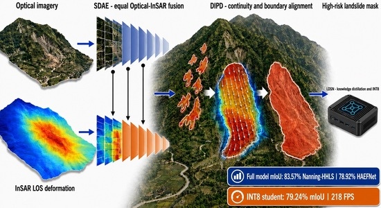
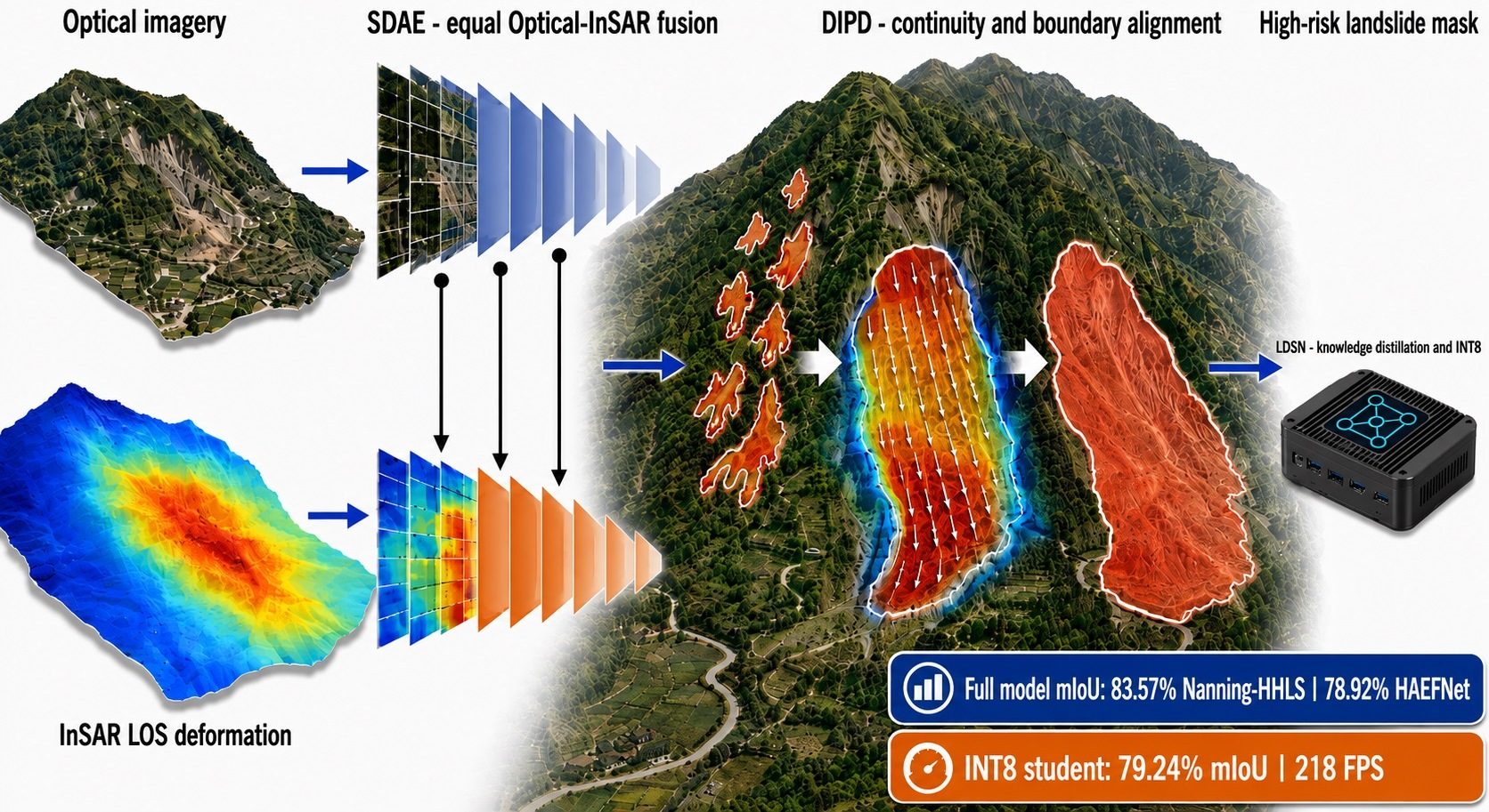
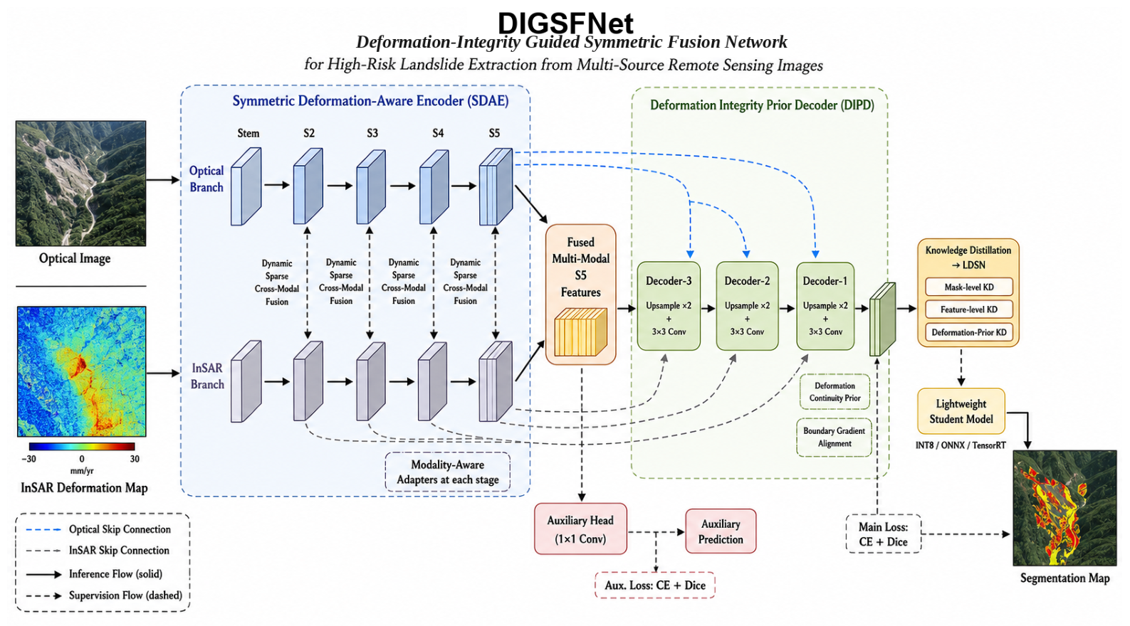
Overall architecture of DIGSFNet, illustrating the three-component pipeline comprising the Symmetric Deformation-Aware Encoder (SDAE), Deformation Integrity Prior Decoder (DIPD), and Lightweight Deployable Student Network (LDSN). Arrows indicate data flow from dual-modal inputs through hierarchical feature extraction, physically-constrained decoding, and knowledge distillation to the final lightweight model.
Figure 1.
Overall architecture of DIGSFNet, illustrating the three-component pipeline comprising the Symmetric Deformation-Aware Encoder (SDAE), Deformation Integrity Prior Decoder (DIPD), and Lightweight Deployable Student Network (LDSN). Arrows indicate data flow from dual-modal inputs through hierarchical feature extraction, physically-constrained decoding, and knowledge distillation to the final lightweight model.
Figure 2.
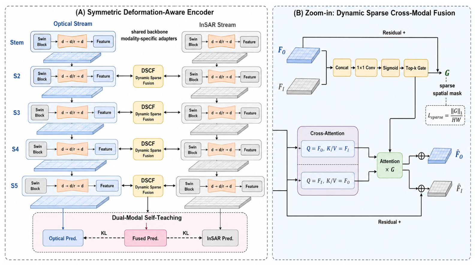
Detailed structure of the Symmetric Deformation-Aware Encoder (SDAE), showing the shared Swin Transformer backbone with modality-specific adapters, the Dynamic Sparse Cross-Modal Fusion modules at each hierarchical stage, and the dual-modal self-teaching supervision pathways.
Figure 2.
Detailed structure of the Symmetric Deformation-Aware Encoder (SDAE), showing the shared Swin Transformer backbone with modality-specific adapters, the Dynamic Sparse Cross-Modal Fusion modules at each hierarchical stage, and the dual-modal self-teaching supervision pathways.
Figure 3.
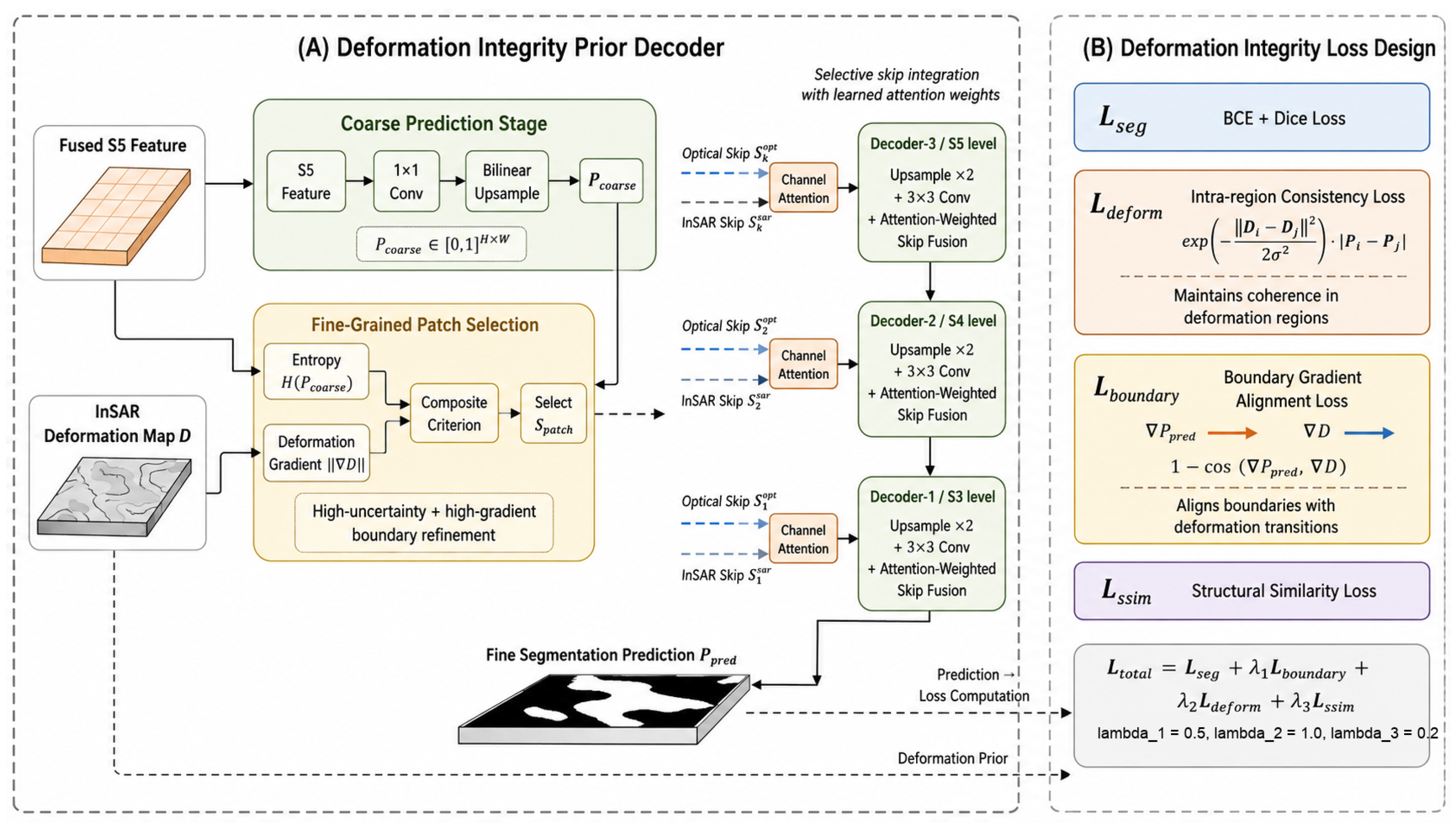
Detailed structure of the Deformation Integrity Prior Decoder (DIPD), illustrating the coarse-to-fine prediction pipeline, fine-grained patch selection based on uncertainty and deformation gradients, multi-scale feature integration with attention-weighted skip connections, and the deformation integrity loss components.
Figure 3.
Detailed structure of the Deformation Integrity Prior Decoder (DIPD), illustrating the coarse-to-fine prediction pipeline, fine-grained patch selection based on uncertainty and deformation gradients, multi-scale feature integration with attention-weighted skip connections, and the deformation integrity loss components.
Figure 4.
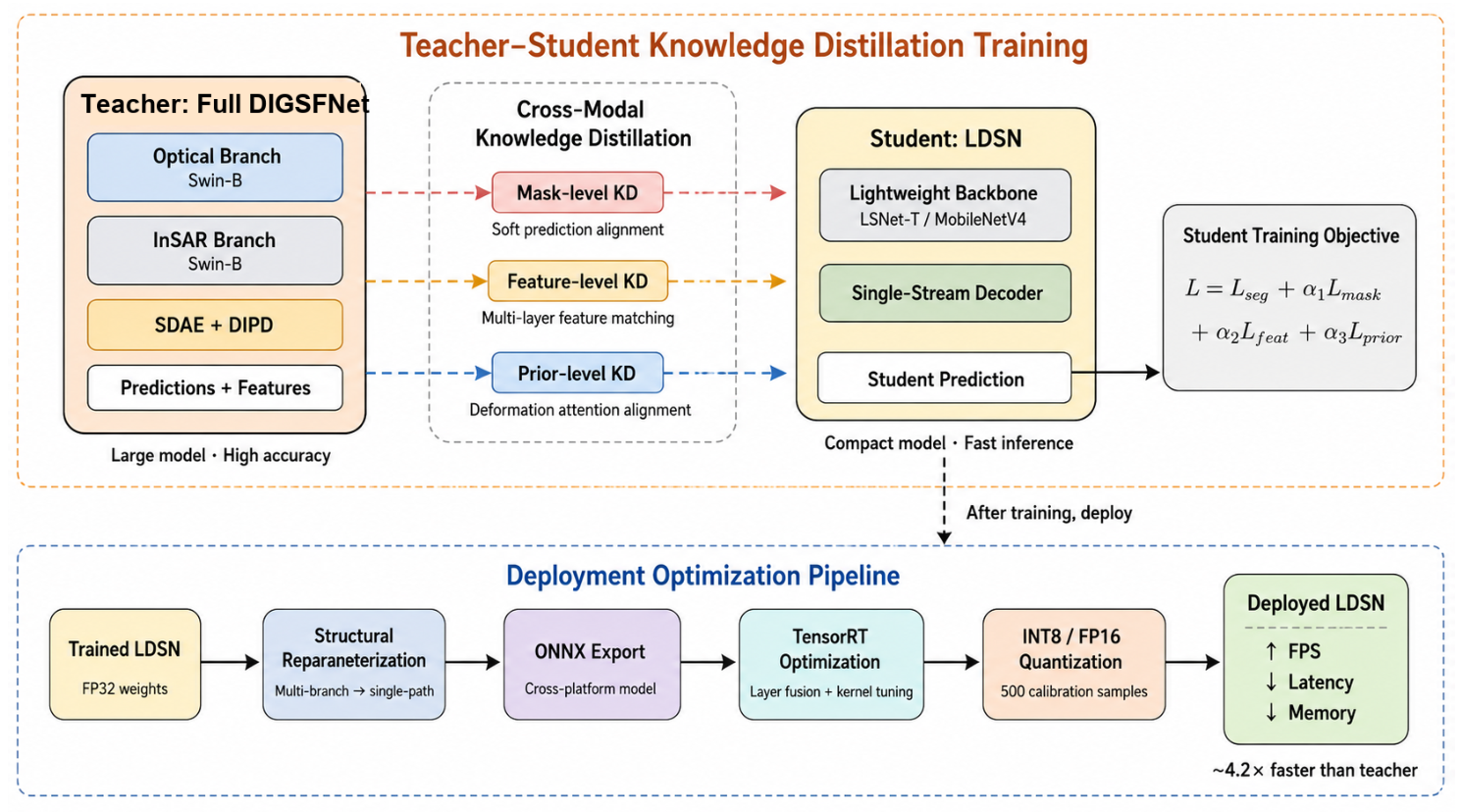
Teacher–student distillation pipeline of the Lightweight Deployable Student Network (LDSN), showing the three-level knowledge transfer (mask-level, feature-level, deformation-prior distillation), the compact student architecture, and the deployment optimization workflow including structural reparameterization, ONNX (opset 17) export, and TensorRT (v8.6) acceleration.
Figure 4.
Teacher–student distillation pipeline of the Lightweight Deployable Student Network (LDSN), showing the three-level knowledge transfer (mask-level, feature-level, deformation-prior distillation), the compact student architecture, and the deployment optimization workflow including structural reparameterization, ONNX (opset 17) export, and TensorRT (v8.6) acceleration.
Figure 5.
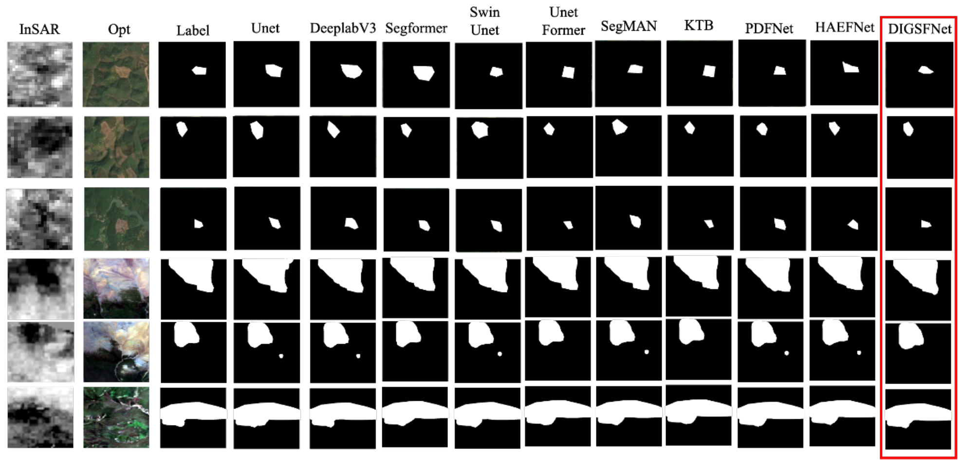
Qualitative comparison visualization across representative challenging scenes from both the Nanning-HHLS and HAEFNet benchmarks. From left to right, each row shows the InSAR LOS deformation map, the optical/RGB context, the ground-truth mask, and the prediction maps from U-Net, DeepLabV3+, SegFormer, Swin-UNet [
54], UNetFormer [
55], SegMAN [
56], KTB, PDFNet, HAEFNet [
5], and DIGSFNet. All predictions are presented as binary masks (white: predicted landslide, black: background). The rightmost column, outlined in red, corresponds to the proposed DIGSFNet.
Figure 5.
Qualitative comparison visualization across representative challenging scenes from both the Nanning-HHLS and HAEFNet benchmarks. From left to right, each row shows the InSAR LOS deformation map, the optical/RGB context, the ground-truth mask, and the prediction maps from U-Net, DeepLabV3+, SegFormer, Swin-UNet [
54], UNetFormer [
55], SegMAN [
56], KTB, PDFNet, HAEFNet [
5], and DIGSFNet. All predictions are presented as binary masks (white: predicted landslide, black: background). The rightmost column, outlined in red, corresponds to the proposed DIGSFNet.
Figure 6.
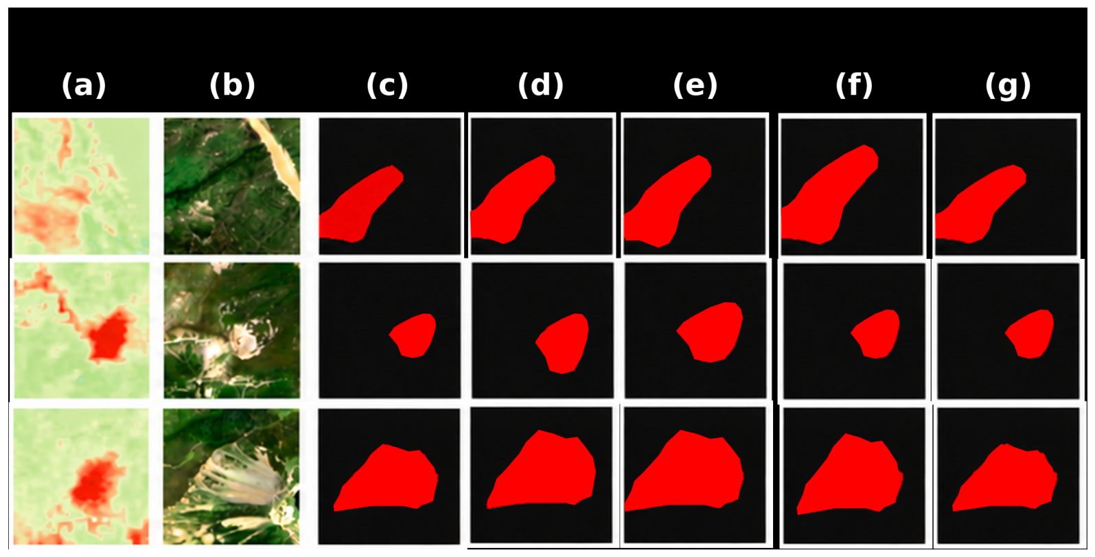
Ablation visualization on challenging scenes. Each scene shows the progressive improvement from (a) InSAR LOS deformation map, (b) optical image, (c) ground truth, (d) optical-only prediction (Config 1), (e) direct concatenation (Config 3), (f) symmetric fusion without DIPD (Config 5), and (g) full DIGSFNet (Config 9).
Figure 6.
Ablation visualization on challenging scenes. Each scene shows the progressive improvement from (a) InSAR LOS deformation map, (b) optical image, (c) ground truth, (d) optical-only prediction (Config 1), (e) direct concatenation (Config 3), (f) symmetric fusion without DIPD (Config 5), and (g) full DIGSFNet (Config 9).
Figure 7.
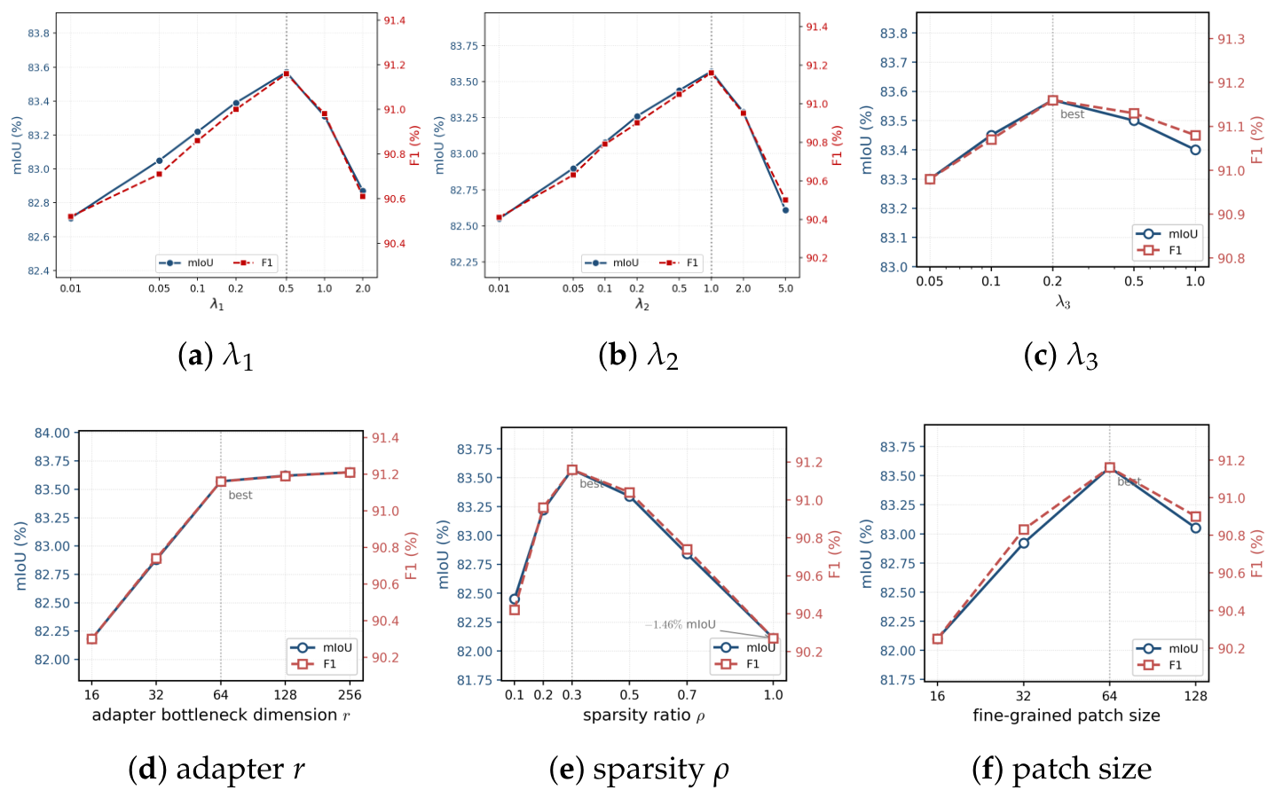
Hyperparameter sensitivity curves. Six subplots arranged in a 2 × 3 grid. Each subplot shows mIoU (solid line with circle markers, left y-axis) and F1 (dashed line with square markers, right y-axis) versus one hyperparameter value; the dotted vertical guide marks the best-performing configuration. (a) varied over ; (b) varied over ; (c) varied over ; (d) adapter bottleneck dimension r varied over ; (e) sparsity ratio varied over ; (f) fine-grained patch size varied over .
Figure 7.
Hyperparameter sensitivity curves. Six subplots arranged in a 2 × 3 grid. Each subplot shows mIoU (solid line with circle markers, left y-axis) and F1 (dashed line with square markers, right y-axis) versus one hyperparameter value; the dotted vertical guide marks the best-performing configuration. (a) varied over ; (b) varied over ; (c) varied over ; (d) adapter bottleneck dimension r varied over ; (e) sparsity ratio varied over ; (f) fine-grained patch size varied over .
Figure 8.
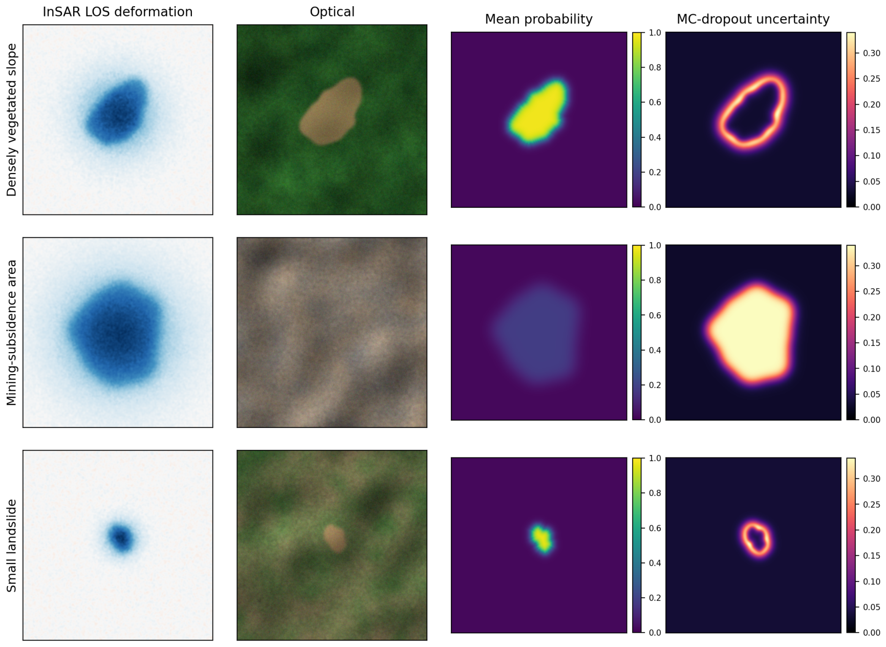
Confidence and uncertainty visualization for representative ambiguous scenes. From left to right, each row shows the InSAR LOS deformation map, the optical context, the predicted probability (confidence) map, and the Monte-Carlo-dropout uncertainty map (30 stochastic forward passes); the figure three rows correspond to a densely vegetated slope, a mining-subsidence area, and a small landslide. Uncertainty concentrates along boundary transition zones and over the non-landslide (mining) deformation source, whereas landslide interiors are predicted with high confidence—consistent with the intended effect of the deformation-integrity priors.
Figure 8.
Confidence and uncertainty visualization for representative ambiguous scenes. From left to right, each row shows the InSAR LOS deformation map, the optical context, the predicted probability (confidence) map, and the Monte-Carlo-dropout uncertainty map (30 stochastic forward passes); the figure three rows correspond to a densely vegetated slope, a mining-subsidence area, and a small landslide. Uncertainty concentrates along boundary transition zones and over the non-landslide (mining) deformation source, whereas landslide interiors are predicted with high confidence—consistent with the intended effect of the deformation-integrity priors.
Table 1.
Comparison of the Nanning-HHLS and HAEFNet datasets used in this study.
Table 1.
Comparison of the Nanning-HHLS and HAEFNet datasets used in this study.
| Attribute | Nanning-HHLS
(This Work) | HAEFNet (Public Benchmark) [5] |
|---|
| Geographic region | Nanning, Guangxi, S China | Qinghai–Tibet Plateau and Sichuan, W China |
| Task | High-risk landslide segmentation | Active landslide detection |
| Input modalities | Optical + InSAR | Optical + InSAR (+DEM, not used) |
| Optical source | Sentinel-2 L2A, 10 bands (10 m) | Sentinel-2 RGB (10 m) |
| InSAR source/product | Sentinel-1 SBAS-InSAR, cumulative LOS displacement | Sentinel-1, mean LOS deformation rate |
| Spatial resolution | 10 m | 10 m |
| Patch size | 512 × 512 px | 512 × 512 px |
| Total patches | 3842 | 8440 |
| Landslide instances | 467 | 1013 |
| Annotation type | Pixel-level binary mask | Pixel-level binary mask |
| Train/Val/Test split | 60/20/20 (spatially stratified) | 7:1:2 (official split) |
Table 2.
Typical magnitude of each weighted loss component at three training stages on Nanning-HHLS (running-average weighted terms).
Table 2.
Typical magnitude of each weighted loss component at three training stages on Nanning-HHLS (running-average weighted terms).
| Weighted Term | Epoch 1 | Epoch 60 | Epoch 120 |
|---|
| 0.812 | 0.214 | 0.128 |
| 0.341 | 0.112 | 0.068 |
| 0.287 | 0.093 | 0.051 |
| 0.124 | 0.047 | 0.029 |
| 0.196 | 0.061 | 0.033 |
| 0.021 | 0.009 | 0.006 |
Table 3.
Quantitative comparison on the Nanning-HHLS dataset. The best results are marked in bold and the second-best results underlined. Bold and underline apply to the accuracy metrics only; the last column (model parameters) is an efficiency measure for which a smaller value is preferable and is therefore left unmarked.
Table 3.
Quantitative comparison on the Nanning-HHLS dataset. The best results are marked in bold and the second-best results underlined. Bold and underline apply to the accuracy metrics only; the last column (model parameters) is an efficiency measure for which a smaller value is preferable and is therefore left unmarked.
| Method | mIoU (%) | F1 (%) | Precision (%) | Recall (%) | AUC (%) | BF1 (%) | Miss. (%) | FA (%) | Params (M) |
|---|
| U-Net | 71.24 | 82.45 | 83.12 | 81.79 | 91.56 | 68.32 | 18.21 | 16.88 | 31.04 |
| DeepLabV3+ | 72.86 | 83.67 | 84.22 | 83.13 | 92.31 | 69.78 | 16.87 | 15.78 | 41.26 |
| SegFormer | 74.53 | 85.01 | 85.67 | 84.36 | 93.12 | 71.45 | 15.64 | 14.33 | 47.28 |
| Swin-UNet | 75.12 | 85.42 | 86.04 | 84.81 | 93.47 | 72.11 | 15.19 | 13.96 | 59.84 |
| UNetFormer | 76.38 | 86.32 | 86.91 | 85.74 | 93.92 | 73.28 | 14.26 | 13.10 | 11.69 |
| SegMAN | 77.92 | 87.42 | 87.83 | 87.01 | 94.56 | 74.86 | 12.99 | 12.18 | 52.37 |
| KTB | 79.14 | 88.29 | 88.52 | 88.06 | 95.03 | 76.04 | 11.94 | 11.48 | 64.22 |
| PDFNet | 80.26 | 89.06 | 89.31 | 88.81 | 95.47 | 77.12 | 11.19 | 10.70 | 71.85 |
| HAEFNet | 80.94 | 89.52 | 89.62 | 89.43 | 95.78 | 77.86 | 10.57 | 10.38 | 76.32 |
| DIGSFNet (Ours) | 83.57 | 91.16 | 90.84 | 91.48 | 96.82 | 82.34 | 8.52 | 9.16 | 88.46 |
Table 4.
Quantitative comparison on the public HAEFNet benchmark [
5]. Same format and methods as
Table 3; the DEM channel is disabled for all methods. The best results are marked in bold and the second-best results underlined. Bold and underline apply to the accuracy metrics only; the last column (model parameters, an efficiency measure) is not marked.
Table 4.
Quantitative comparison on the public HAEFNet benchmark [
5]. Same format and methods as
Table 3; the DEM channel is disabled for all methods. The best results are marked in bold and the second-best results underlined. Bold and underline apply to the accuracy metrics only; the last column (model parameters, an efficiency measure) is not marked.
| Method | mIoU (%) | F1 (%) | Precision (%) | Recall (%) | AUC (%) | BF1 (%) | Miss. (%) | FA (%) | Params (M) |
|---|
| U-Net | 67.12 | 79.84 | 80.42 | 79.27 | 89.84 | 64.18 | 20.73 | 19.58 | 31.04 |
| DeepLabV3+ | 68.83 | 81.05 | 81.62 | 80.49 | 90.51 | 65.74 | 19.51 | 18.38 | 41.26 |
| SegFormer | 70.62 | 82.38 | 82.89 | 81.88 | 91.27 | 67.43 | 18.12 | 17.11 | 47.28 |
| Swin-UNet | 71.45 | 82.92 | 83.51 | 82.34 | 91.68 | 68.21 | 17.66 | 16.49 | 59.84 |
| UNetFormer | 72.34 | 83.59 | 84.08 | 83.11 | 92.06 | 69.27 | 16.89 | 15.92 | 11.69 |
| SegMAN | 73.58 | 84.42 | 84.81 | 84.04 | 92.71 | 70.62 | 15.96 | 15.19 | 52.37 |
| KTB | 74.62 | 85.13 | 85.42 | 84.85 | 93.18 | 71.85 | 15.15 | 14.58 | 64.22 |
| PDFNet | 75.18 | 85.51 | 85.74 | 85.28 | 93.46 | 72.43 | 14.72 | 14.26 | 71.85 |
| HAEFNet | 75.24 | 85.84 | 85.92 | 85.76 | 93.62 | 73.18 | 14.24 | 14.08 | 76.32 |
| DIGSFNet (Ours) | 78.92 | 88.14 | 87.95 | 88.34 | 95.04 | 78.45 | 11.66 | 12.05 | 88.46 |
Table 5.
Ablation study results on the Nanning-HHLS dataset. Within the teacher variants (Configs 1–9) and the student variants (Configs 10–11), the best value in each accuracy column is shown in bold; the parameters and FLOPs columns (efficiency measures) are not marked.
Table 5.
Ablation study results on the Nanning-HHLS dataset. Within the teacher variants (Configs 1–9) and the student variants (Configs 10–11), the best value in each accuracy column is shown in bold; the parameters and FLOPs columns (efficiency measures) are not marked.
| Configuration | mIoU (%) | F1 (%) | Recall (%) | BF1 (%) | Params (M) | FLOPs (G) |
|---|
| (1) Optical only | 74.12 | 85.18 | 82.15 | 66.48 | 85.34 | 197.6 |
| (2) InSAR only | 71.85 | 83.56 | 79.42 | 62.78 | 85.34 | 197.6 |
| (3) Optical + InSAR direct concatenation | 76.42 | 86.64 | 83.68 | 68.92 | 85.42 | 198.9 |
| (4) Asymmetric fusion (InSAR as auxiliary) | 78.56 | 87.92 | 85.41 | 71.34 | 86.78 | 208.3 |
| (5) Symmetric fusion (SDAE, w/o DIPD) | 81.03 | 89.53 | 88.56 | 76.82 | 87.62 | 211.2 |
| (6) Full model w/o deformation integrity loss | 81.86 | 89.98 | 89.87 | 78.12 | 88.46 | 215.8 |
| (7) Full model w/o fine-grained patch decoder | 82.64 | 90.52 | 90.68 | 79.45 | 87.85 | 211.2 |
| (8) Full model w/o self-teaching | 82.15 | 90.26 | 90.23 | 81.08 | 88.46 | 215.8 |
| (9) Full DIGSFNet (teacher) | 83.57 | 91.16 | 91.48 | 82.34 | 88.46 | 215.8 |
| (10) LDSN (student, w/o distillation) | 76.48 | 86.68 | 84.12 | 72.58 | 11.32 | 27.6 |
| (11) LDSN (student, with full distillation) | 79.92 | 88.79 | 87.96 | 77.84 | 11.32 | 27.6 |
Table 6.
Ablation of the three distillation levels on the Nanning-HHLS dataset (student = LSNet-T). The best value in each column is shown in bold.
Table 6.
Ablation of the three distillation levels on the Nanning-HHLS dataset (student = LSNet-T). The best value in each column is shown in bold.
| Distillation Configuration | mIoU (%) | F1 (%) | Recall (%) | BF1 (%) |
|---|
| None (Config 10) | 76.48 | 86.68 | 84.12 | 72.58 |
| Mask-level only | 77.81 | 87.41 | 85.63 | 74.06 |
| Feature-level only | 77.95 | 87.53 | 85.81 | 74.39 |
| Deformation-prior only | 78.16 | 87.66 | 85.44 | 75.90 |
| Mask + feature | 78.84 | 88.21 | 86.99 | 75.60 |
| Full three-level (Config 11) | 79.92 | 88.79 | 87.96 | 77.84 |
Table 7.
Efficiency comparison between teacher and student models. All inference metrics measured on a single RTX 4090 GPU with input.
Table 7.
Efficiency comparison between teacher and student models. All inference metrics measured on a single RTX 4090 GPU with input.
| Model | Params (M) | FLOPs (G) | FPS | ONNX (ms) | INT8 (ms) | GPU Mem. (GB) | mIoU (%) | F1 (%) |
|---|
| DIGSFNet Teacher (FP32) | 88.46 | 215.8 | 18 | 54.2 | — | 4.85 | 83.57 | 91.16 |
| LDSN Student (FP32) | 11.32 | 27.6 | 76 | 13.2 | — | 1.24 | 79.92 | 88.79 |
| LDSN Student (FP16) | 11.32 | 27.6 | 142 | 7.1 | — | 0.82 | 79.86 | 88.74 |
| LDSN Student (INT8) | 11.32 | 27.6 | 218 | — | 4.6 | 0.54 | 79.24 | 88.31 |
Table 8.
Repeated-run statistics (mean ± std over 3 seeds) and significance of the DIGSFNet–HAEFNet comparison.
Table 8.
Repeated-run statistics (mean ± std over 3 seeds) and significance of the DIGSFNet–HAEFNet comparison.
| Dataset | DIGSFNet mIoU (%) | HAEFNet mIoU (%) | p-Value |
|---|
| Nanning-HHLS | 83.57 ± 0.18 | 80.94 ± 0.21 | <0.01 |
| HAEFNet benchmark | 78.92 ± 0.24 | 75.24 ± 0.27 | <0.01 |




 ,
,