KSR-Huber: A Robust Method for Wind Vector Retrieval from Doppler Wind Lidar Observations

Highlights

What are the main findings?

• KNN–Sigmoid Prior Reweighting (KSR) quantifies local statistical consistency via a KNN-based strategy and performs continuous sigmoid-based prior reweighting.
• A unified KSR-Huber framework couples continuous prior weighting with Huber IRLS residual reweighting to suppress anomalies and preserve valid observations.

What are the implications of the main findings?

• KSR reduces reliance on strong priors and alleviates sensitivity to initial least-squares estimates, improving retrieval stability.
• The proposed method improves robustness and stability in wind vector retrieval under noisy and sparse observations without hard-thresholding, enabling smooth and consistent weighting of measurements.

Abstract

Three-dimensional wind vector retrieval from Coherent Doppler Wind Lidar (CDWL) in Velocity–Azimuth Display (VAD) mode is susceptible to anomalous radial velocity observations induced by low signal-to-noise ratios, clutter echoes, and spectral estimation errors, which degrade inversion accuracy. To address this issue, a robust retrieval method, termed KSR-Huber, is proposed by integrating K-nearest-neighbor (KNN)-based local statistical priors with Huber iterative reweighted least squares (IRLS). The method employs KNN-based local consistency and adaptive Sigmoid weighting, together with Huber residual reweighting within the IRLS framework, to suppress anomalous observations while preserving valid data. Simulations across diverse scenarios, conducted under controlled numerical experiments with varying observation redundancies and outlier contamination levels, show that the proposed method consistently outperforms existing approaches, including DSWF, KNN-COOKS, and airSWF, particularly in terms of robustness under controlled noise and outlier conditions. Real lidar observations further demonstrate the practical applicability of the method, while comprehensive validation against independent reference measurements is left for future work.

1. Introduction

Coherent Doppler wind lidar (CDWL) has been widely used in wind energy assessment, wake analysis, atmospheric turbulence, and dynamic process studies, owing to its high spatiotemporal resolution and non-contact measurement capability [1,2]. CDL obtains line-of-sight radial wind speeds by detecting the Doppler shift in laser echoes and requires integrating data from multiple directions to retrieve three-dimensional wind vectors [3]. However, in practical observations, radial velocity data are often contaminated by noise and outliers due to factors like low signal-to-noise ratios [4], uneven aerosol distributions, and instrumental errors, which substantially degrade the accuracy and robustness of the retrieval [5,6].

To enhance the accuracy and robustness of wind field retrieval, various methods have been proposed in prior studies [7]. Direct sine wave fitting (DSWF) relies on least-squares fitting of radial velocities but is highly sensitive to noise and outliers [8]. Building on this, filtered sine wave fitting (FSWF) incorporates prior information (e.g., signal-to-noise ratios) for data screening to improve stability [9], though its performance hinges on threshold settings and risks discarding valid observations. Furthermore, the adaptive iterative reweighted sine wave fitting method (airSWF) employs residual-based iterative weighting to replace hard filtering with continuous weights [10], but its effectiveness is limited by the quality of initial fits. Subsequently, the weighted sine wave fitting algorithm based on K-nearest neighbors and Cook’s distance (KNN-COOKS) leverages local statistical information to capture spatial consistency and improve outlier detection [11], but it still relies on discrete discrimination or threshold mechanisms, which limits its flexibility under complex conditions. Overall, existing methods for robust wind field retrieval face three common challenges: (1) strong dependence on prior information or initial estimates, which can lead to unstable results; (2) weighting strategies often based on discrete discrimination or hard-threshold mechanisms, lacking continuous adaptive capabilities; and (3) absence of a unified robust modeling framework to jointly capture local consistency and residual reliability.

To address these issues, this paper proposes a coupled weighting method called KSR-Huber, which integrates K-nearest-neighbor-based local statistical priors with Huber iterative reweighted least squares (IRLS) to achieve continuous, adaptive weighting and thereby enhance the robustness and stability of wind vector retrieval under noisy and sparse observational conditions. The method is evaluated using real lidar observations to demonstrate its practical applicability under the investigated conditions; a broader evaluation covering additional dates and atmospheric regimes, together with a benchmark against independent reference measurements, will be conducted in future work. The main contributions of this paper are as follows:

1.

A K-nearest-neighbor-based local statistical weighting strategy is proposed to reduce reliance on hard filtering thresholds and alleviate sensitivity to initial estimates, thereby improving the stability of wind vector retrieval;

2.

A continuous adaptive weighting mechanism is developed by combining a sigmoid-based prior weight function with Huber iterative reweighted least squares (IRLS), effectively overcoming the limitations of discrete discrimination or hard-threshold weighting;

3.

A unified coupled robust framework, KSR-Huber, is introduced to jointly model local data consistency and residual reliability, enabling robust wind vector retrieval under noisy and sparse observations.

2. Principle

2.1. Principle of Wind Vector Retrieval

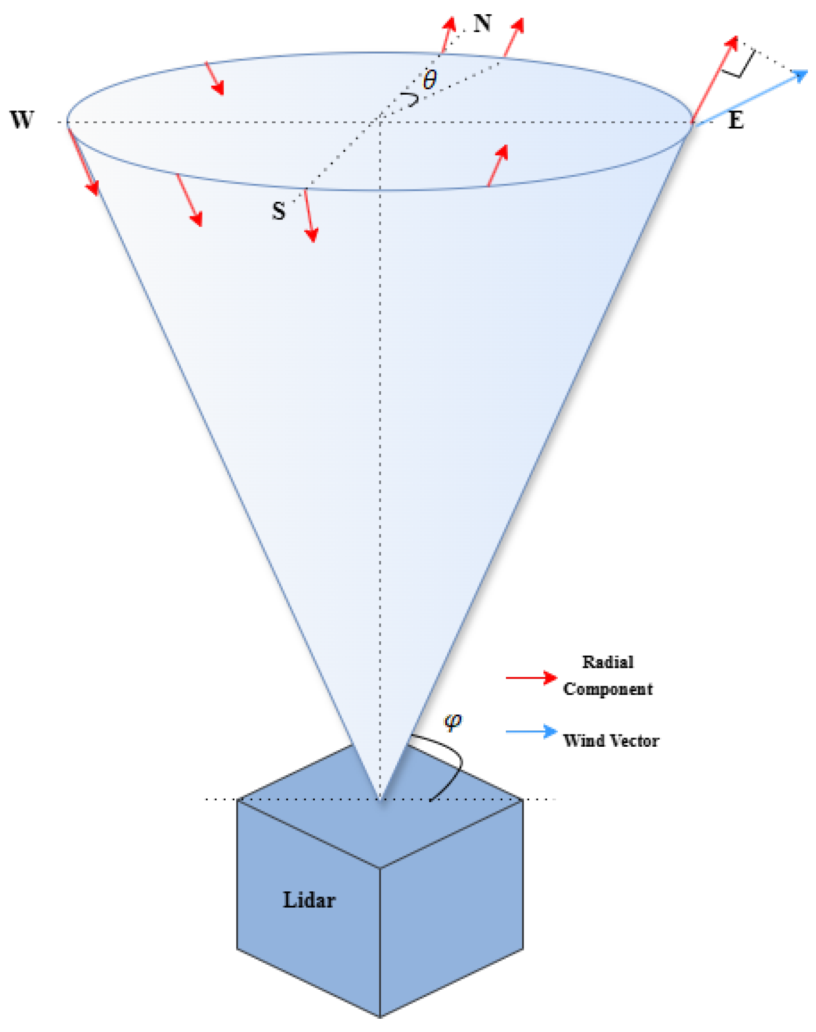
This study uses coherent Doppler wind lidar (CDWL) and the Velocity–Azimuth Display (VAD) principle to infer the three-dimensional wind vector from multiple radial wind velocity measurements ($V_r$) [12]. As shown in Figure 1, fixed-elevation-angle scanning is adopted: at a constant elevation angle ($\varphi$), namely $\varphi$ is measured upward from the horizontal plane, the lidar samples multiple azimuth angles (${\theta }_i$), providing radial wind speed observations at the same height for wind-vector estimation [13]. In VAD mode, the elevation angle is kept constant (e.g., $\varphi ={60}^{\circ }$), while the azimuth angles (${\theta }_i$) span $0^{\circ }$–${360}^{\circ }$. For each ${\theta }_i$ and $\varphi$, the radial wind speed ($V_{r,i}$) is estimated and, under the assumption of horizontally uniform and quasi-steady wind at the same height during a scanning cycle, varies sinusoidally with azimuth angle, forming the basis of the VAD retrieval [14,15]. Let the three-dimensional wind vector be represented as

$$\mathbf{V}=\left[\begin{array}{c}u\\ v\\ w\end{array}\right],$$

(1)

where u and v are the horizontal wind components in the east (E) and north (N) directions, respectively, and w is the vertical wind component. For the i-th azimuth observation angle ${\theta }_i$ at a fixed elevation angle $\varphi$, the corresponding line-of-sight unit vector can be written as

$${\mathbf{s}}_i=\left[\begin{array}{c}sin\left({\theta }_i\right)cos\left(\varphi \right)\\ cos\left({\theta }_i\right)cos\left(\varphi \right)\\ sin\left(\varphi \right)\end{array}\right].$$

(2)

The radial wind speed is defined as the projection of the wind vector onto the line-of-sight direction

$$V_{r,i}={\mathbf{V}}^{\mathsf{T}}{\mathbf{s}}_i=usin\left({\theta }_i\right)cos\left(\varphi \right)+vcos\left({\theta }_i\right)cos\left(\varphi \right)+wsin\left(\varphi \right).$$

(3)

Introducing the horizontal wind speed $V_h=\sqrt{u^2+v^2}$ and the horizontal wind direction $\psi$, the equation can be equivalently expressed as the VAD sinusoidal model

$$V_r\left(\theta \right)=V_{h}cos(\theta -\psi )+wsin\left(\varphi \right).$$

(4)

When $\varphi$ is large (i.e., $\varphi \to {90}^{\circ }$ so that the beam approaches the zenith direction), $cos\left(\varphi \right)$ decreases, reducing the sensitivity of $V_r$ to the horizontal wind components. Conversely, when $\varphi$ is small, the contribution of the vertical component $wsin\left(\varphi \right)$ becomes weaker. Therefore, a compromise elevation angle is commonly selected.

When $\varphi$ is large (close to zenith), $cos\left(\varphi \right)$ decreases, reducing the sensitivity of $V_r$ to the horizontal wind components. Conversely, when $\varphi$ is small, the contribution of the vertical component $wsin\left(\varphi \right)$ becomes weaker. Therefore, a compromise elevation angle is commonly selected.

2.1.1. Least-Squares Method

In wind field measurements, radial wind speeds from multiple azimuth angles are used to retrieve the wind vector [16]. In the VAD method, the retrieval can be formulated as an overdetermined system

$${\mathbf{V}}_r=\mathbf{A}\mathbf{v}.$$

(5)

where ${\mathbf{V}}_r={[V_{r,1},V_{r,2},\dots ,V_{r,n}]}^T$ collects radial wind speed observations at n azimuth angles, and $\mathbf{v}={[u,v,w]}^T$ is the three-dimensional wind vector to be estimated [17]. The design matrix $\mathbf{A}$ is

$$\mathbf{A}=\left(\begin{array}{ccc}sin{\theta }_{1}cos\varphi & cos{\theta }_{1}cos\varphi & sin\varphi \\ ⋮& ⋮& ⋮\\ sin{\theta }_{n}cos\varphi & cos{\theta }_{n}cos\varphi & sin\varphi \end{array}\right).$$

(6)

For an overdetermined system, the wind vector retrieval is solved by least squares by minimizing the residual norm

$$\underset{\mathbf{V}}{min}{∥{\mathbf{V}}_r-\mathbf{A}\mathbf{V}∥}_2^2.$$

(7)

Specifically, the normal equation can be constructed

$${\mathbf{A}}^{\mathsf{T}}\mathbf{A}\mathbf{V}={\mathbf{A}}^{\mathsf{T}}{\mathbf{V}}_r.$$

(8)

The least-squares solution for the wind vector is then given by

$$\mathbf{V}={\left({\mathbf{A}}^{\mathsf{T}}\mathbf{A}\right)}^{-1}{\mathbf{A}}^{\mathsf{T}}{\mathbf{V}}_r.$$

(9)

The above solution serves as the unweighted baseline for the subsequent weighted least-squares framework. In Section 2.1.2, a diagonal weight matrix is introduced to account for heterogeneous reliability and outliers, which are further addressed by the proposed KSR-Huber scheme in Section 3.

2.1.2. Weighted Least-Squares Method

In practical wind vector retrieval, radial wind-speed observations from different azimuth angles may have non-uniform reliability due to noise and outliers [18], which can degrade the unweighted least-squares solution.

To enhance robustness, we use a weighted least-squares (WLS) scheme to reduce the impact of measurement errors [19]. Each observation is assigned a weight according to its reliability, where interference-contaminated data receive smaller weights and more reliable measurements are weighted higher to exert greater influence on the retrieved wind vector [20].

The weighted least-squares method obtains the optimal solution by minimizing the weighted sum of squared residuals

$$\underset{\mathbf{V}}{min}{∥{\mathbf{W}}^{1/2}\left({\mathbf{V}}_r-\mathbf{A}\mathbf{V}\right)∥}_2^2.$$

(10)

Taking the derivative with respect to $\mathbf{V}$ and setting it to zero yields the weighted normal equation

$${\mathbf{A}}^{\mathsf{T}}\mathbf{W}\mathbf{A}\mathbf{V}={\mathbf{A}}^{\mathsf{T}}\mathbf{W}{\mathbf{V}}_r.$$

(11)

Assuming ${\mathbf{A}}^{\mathsf{T}}\mathbf{W}\mathbf{A}$ is invertible, the analytical solution is given by

$$\mathbf{V}={\left({\mathbf{A}}^{\mathsf{T}}\mathbf{W}\mathbf{A}\right)}^{-1}{\mathbf{A}}^{\mathsf{T}}\mathbf{W}{\mathbf{V}}_r.$$

(12)

where $\mathbf{W}$ represents an $n\times n$ diagonal matrix, with the diagonal elements denoting the weights corresponding to the radial wind-speed observations at each azimuth direction.

3. KSR-Huber Algorithm

3.1. Method Overview

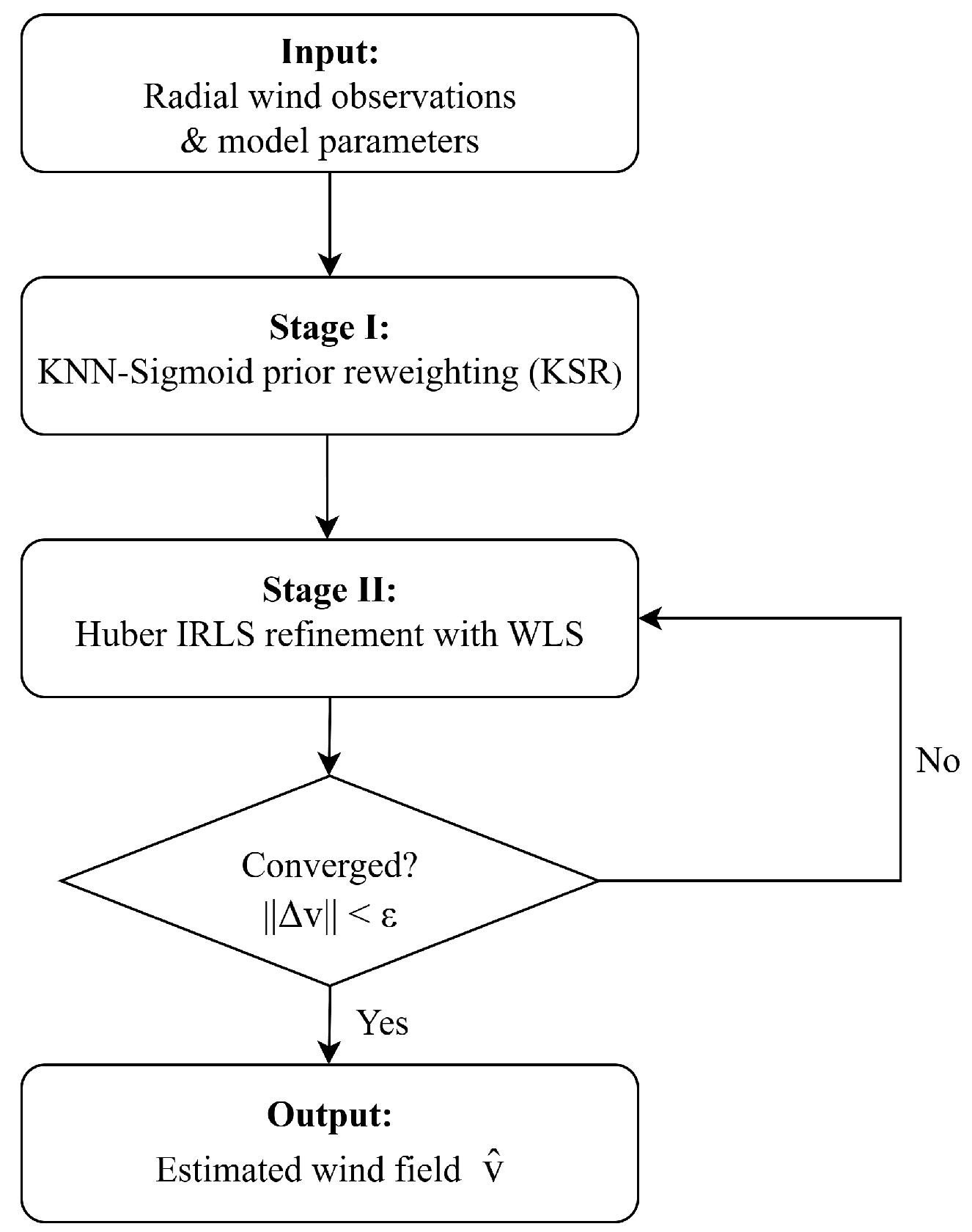
In this study, we propose a two-stage robust wind vector retrieval algorithm, referred to as KSR-Huber (KNN-based Sigmoid Reweighting with Huber IRLS). The method is formulated within a weighted least-squares inversion framework and suppresses anomalous radial wind speeds through two coupled mechanisms: KNN-based prior reweighting and Huber IRLS residual reweighting. The complete process is illustrated in Figure 2.

Specifically, in the first stage (steps b–e), the algorithm employs the K-nearest neighbors (KNN) approach to compute the average absolute difference between each observation and its localized neighborhood in the original radial wind space. This calculation constructs a normalized deviation based on local scales, resulting in a comprehensive outlier degree index. This index is then smoothly mapped to a continuous prior weight in the range of [0, 1] using a Sigmoid function, effectively mitigating the impact of severe outliers while avoiding information loss associated with hard thresholding.

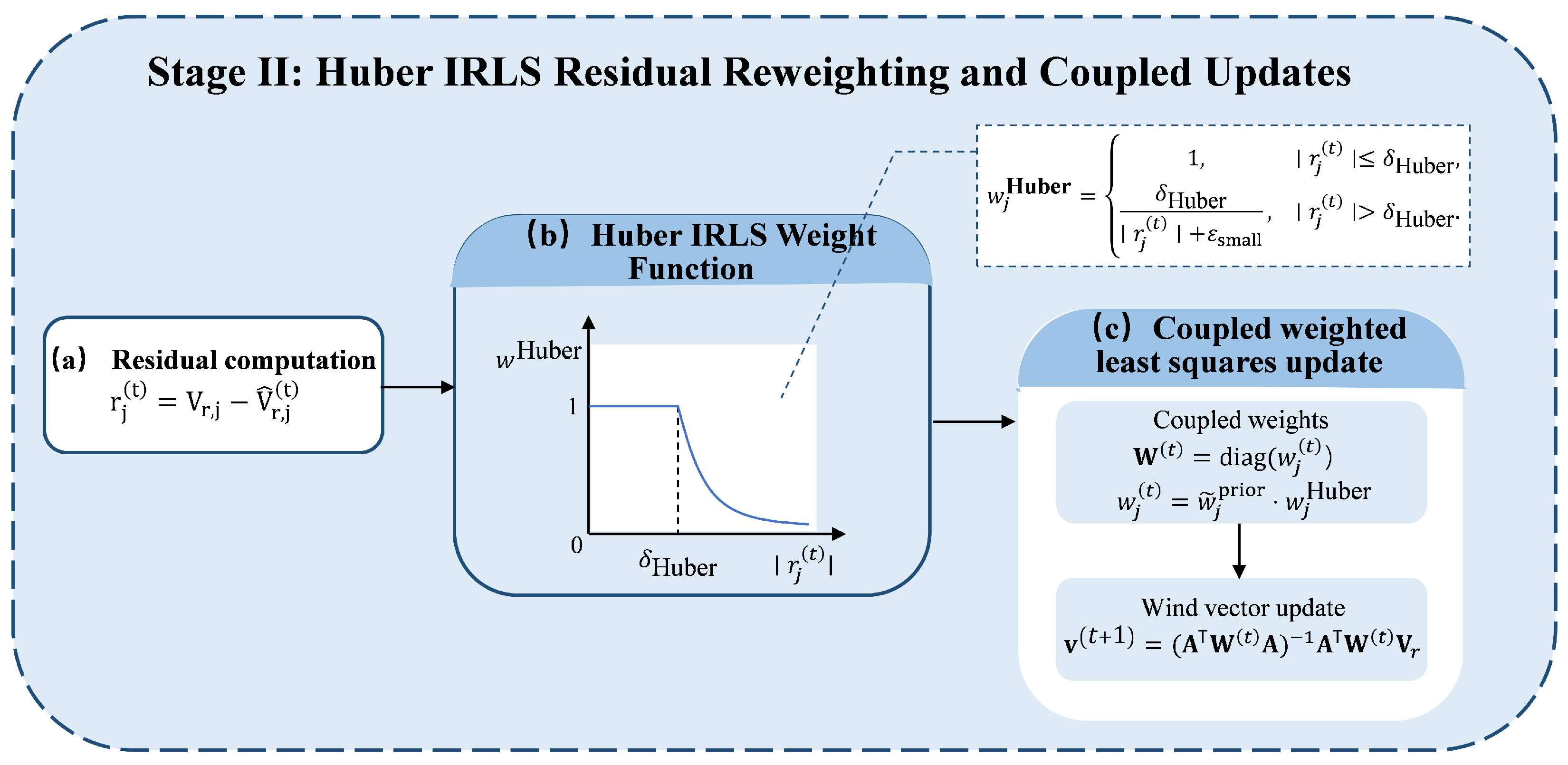
In the second stage (steps f–h), based on the prior weights, we introduce the Huber loss and apply the Iteratively Reweighted Least Squares (IRLS) method to further down-weight observations with large residuals. This ensures that the algorithm can converge to a wind vector solution that balances both accuracy and robustness, even in the presence of strong anomalies, within a finite number of iterations.

3.2. Stage I: KNN–Sigmoid Prior Reweighting (KSR)

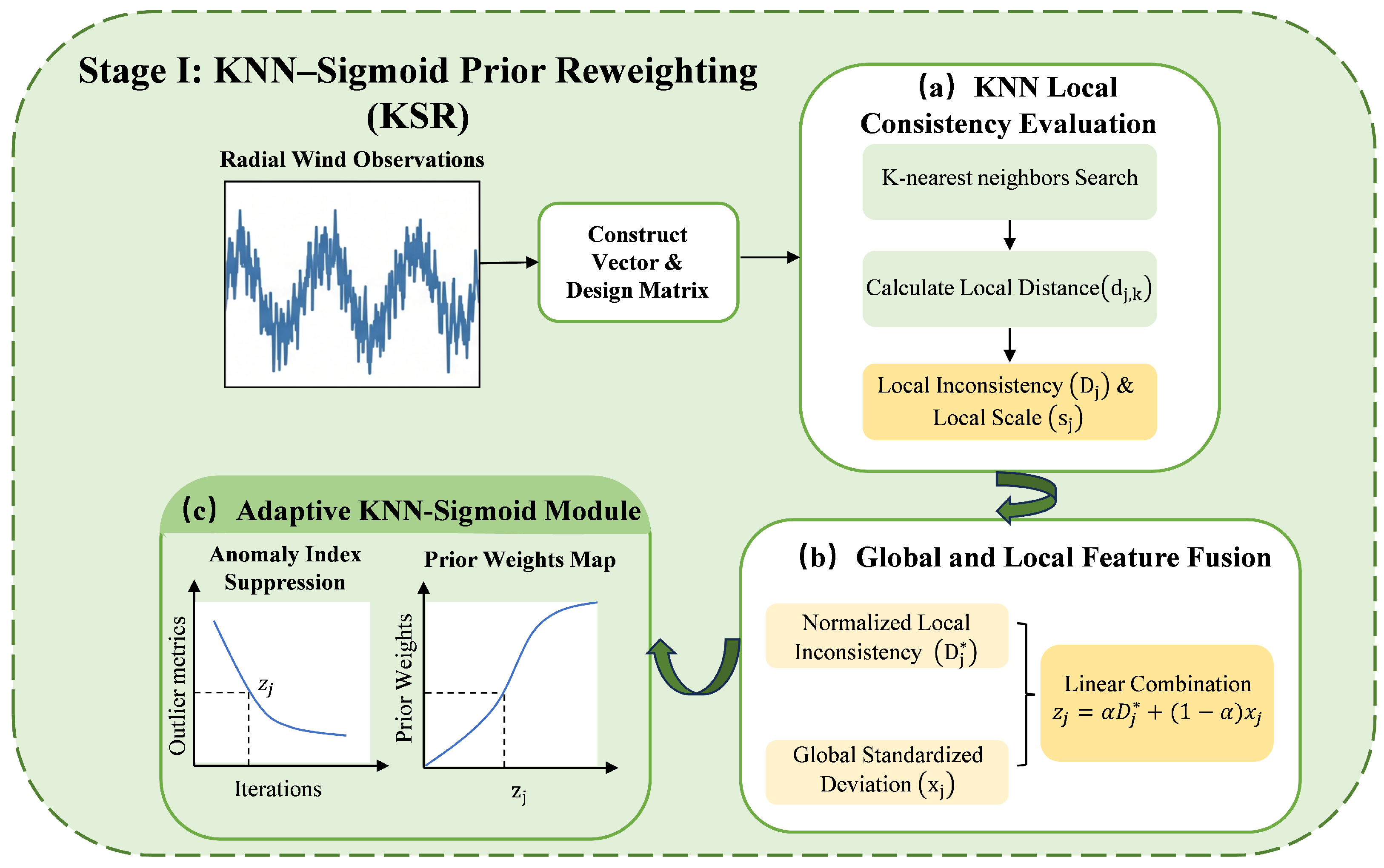
Figure 3 illustrates the three modules of Stage I (KSR): (a) local inconsistency and scale evaluation, (b) global–local feature fusion, and (c) adaptive KNN–Sigmoid mapping.

a. Let the radial wind speed observation vector at a specific height layer obtained in n azimuth directions be

$${\mathbf{V}}_r={(V_{r,1},V_{r,2},\dots ,V_{r,n})}^{\mathsf{T}},$$

(13)

where $V_{r,j}$ denotes the radial wind speed at the j-th azimuth. Based on the elevation and azimuth angles, we construct a direction cosine matrix $\mathbf{A}\in {\mathbb{R}}^{n\times 3}$, where each row corresponds to the unit vector in the respective direction. We initialize the observation weight vector as ${\mathbf{w}}^{\mathrm{KNN}}={(1,\dots ,1)}^{\mathsf{T}}$ and prepare a small constant ${\epsilon }_{\mathrm{small}}={10}^{-8}$ to prevent division by zero.

b. For each observation point $j=1,\dots ,n$, we assess its consistency with neighboring samples using a K-nearest neighbors (KNN) strategy. Specifically, the neighborhood is defined globally in the radial velocity space. We exclude the point itself and compute the absolute differences between the current observation and all other samples

$$d_{j,k}=\mid V_{r,j}-V_{r,k}\mid ,k\ne j.$$

(14)

These values are sorted in ascending order, and the smallest $K_{\mathrm{neighbor}}$ values (in this study, $K_{\mathrm{neighbor}}=5$) are selected, denoted as ${\left\{d_{j,k}\right\}}_{k=1}^{K_{\mathrm{neighbor}}}$. This corresponds to selecting samples with the most similar radial velocities across all azimuth directions, without imposing explicit constraints in the azimuthal domain.

Based on the selected neighbors, the local inconsistency is defined as

$$D_j={\displaystyle \frac{1}{K_{\mathrm{neighbor}}}}{\displaystyle \sum _{k=1}^{K_{\mathrm{neighbor}}}}{d}_{j,k},$$

(15)

where a larger value indicates a more significant discrepancy between the observation and its nearest samples, suggesting that it may be an anomalous observation. Simultaneously, we define the local scale as

$$s_j={\displaystyle \underset{k=1}{\overset{K_{\mathrm{neighbor}}}{max}}}{d}_{j,k},$$

(16)

where $s_j$ serves as the local normalization scale and is subject to a lower bound to ensure numerical stability. Accordingly, $D_j$ and $s_j$ are computed as shown in Figure 3a.

It is worth noting that, although the KNN neighborhood is defined in the radial velocity space, the radial velocity in VAD scans follows a smooth sinusoidal variation with respect to azimuth angle. As a result, samples with similar radial velocities are typically associated with nearby azimuth angles. Therefore, this strategy implicitly preserves azimuthal continuity while avoiding the need for explicit angular constraints.This design also avoids potential sensitivity to uneven angular sampling.

c. To simultaneously consider local consistency and overall distribution, we first robustly normalize the set $\left\{D_j\right\}$. Let the median be defined as

$$D_{\mathrm{med}}=\mathrm{median}\left(D_j\right),$$

(17)

and if $D_{\mathrm{med}}$ is too small, we set $D_{\mathrm{med}}=1$. Thus, we obtain the normalized local inconsistency

$$D_j^{*}={\displaystyle \frac{D_j}{D_{\mathrm{med}}}}.$$

(18)

On the other hand, using the median of all radial wind observations as a reference, defined as ${\tilde{V}}_r=\mathrm{median}\left(V_r\right)$, where ${\tilde{V}}_r$ provides a robust reference against outliers, we construct a standardized deviation based on the local scale

$$x_j={\displaystyle \frac{\left|V_{r,j}-{\tilde{V}}_r\right|}{s_j+{\epsilon }_{\mathrm{small}}}}.$$

(19)

Here, $D_j^{*}$ describes the local neighborhood consistency, while $x_j$ indicates the degree of deviation relative to the overall distribution.

d. The two outlier metrics $D_j^{*}$ and $x_j$ are linearly combined as

$$z_j=\alpha D_j^{*}+(1-\alpha )x_j,\alpha \in [0,1],$$

(20)

where the weight coefficient $\alpha$ balances local information with overall deviation. A larger $z_j$ indicates that the observation exhibits stronger anomalous characteristics on both local and global scales (in this study, we set $\alpha =0.7$). The fused outlier index $z_j$ in Figure 3b is obtained by linearly combining $D_j^{*}$ and $x_j$.

e. To avoid the non-differentiability and irreversibility issues associated with hard thresholds, the comprehensive outlier index $z_j$ is mapped to continuous prior weights using a parameterized Sigmoid function

$$w_j^{\mathrm{prior}}={\displaystyle \frac{1}{1+exp\left({\sigma }_a(z_j-{\sigma }_b)\right)}}.$$

(21)

As depicted in Figure 3c, $z_j$ is mapped to continuous prior weights via an adaptive KNN–Sigmoid function.

Where $w_j^{\mathrm{prior}}\in (0,1)$ and is monotonically decreasing with respect to $z_j$ (when ${\sigma }_a>0$). Here, ${\sigma }_a$ controls the slope of the Sigmoid curve, and ${\sigma }_b$ is the threshold for the weight to drop to 0.5. Based on sensitivity analysis, we select ${\sigma }_a=0.3$ and ${\sigma }_b=1.2$, ensuring that weights begin to decline significantly when $z_j$ approaches 1, while maintaining a gentle variation in the range of small to moderate outlier indices. To prevent a few extremely low weights from leading to ill-conditioned normal equations, we further impose a lower limit on the weights

$$w_j^{\mathrm{prior}}\leftarrow max\left(w_j^{\mathrm{prior}},w_{\min }\right),w_{\min }=0.3.$$

(22)

3.3. Stage II: Huber IRLS Residual Reweighting and Coupled Updates

Figure 4 illustrates the three modules of Stage II: (a) residual computation, (b) Huber IRLS weight function, and (c) coupled weighted least-squares update.

f. After obtaining the prior weights, we introduce the Huber loss to apply secondary weighting on the fitting residuals. First, using the normalized prior weights ${\left\{{\tilde{w}}_j^{\mathrm{prior}}\right\}}_{j=1}^n$, we construct the diagonal weight matrix

$${\mathbf{W}}^{\mathrm{prior}}=\mathrm{diag}({\tilde{w}}_1^{\mathrm{prior}},\dots ,{\tilde{w}}_n^{\mathrm{prior}}).$$

(23)

We then obtain the initial wind vector estimate using the weighted least squares approach

$${\mathbf{v}}^{\left(0\right)}=arg\underset{\mathbf{v}}{min}{({\mathbf{V}}_r-\mathbf{A}\mathbf{v})}^{\mathsf{T}}{\mathbf{W}}^{\mathrm{prior}}({\mathbf{V}}_r-\mathbf{A}\mathbf{v})={\left({\mathbf{A}}^{\mathsf{T}}{\mathbf{W}}^{\mathrm{prior}}\mathbf{A}\right)}^{-1}{\mathbf{A}}^{\mathsf{T}}{\mathbf{W}}^{\mathrm{prior}}{\mathbf{V}}_r.$$

(24)

In the t-th iteration, the fitted radial wind values and residuals are computed as

$${\widehat{\mathbf{V}}}_r^{\left(t\right)}=\mathbf{A}{\mathbf{v}}^{\left(t\right)},$$

(25)

$$r_j^{\left(t\right)}=V_{r,j}-{\widehat{V}}_{r,j}^{\left(t\right)}.$$

(26)

Given the Huber threshold ${\delta }_{\mathrm{Huber}}=1.3$, we construct the residual weights

$$w_j^{\mathrm{Huber}}=\left\{\begin{array}{cc}1,\hfill & \left|r_j^{\left(t\right)}\right|\le {\delta }_{\mathrm{Huber}},\hfill \\ {\displaystyle \frac{{\delta }_{\mathrm{Huber}}}{\left|r_j^{\left(t\right)}\right|+{\epsilon }_{\mathrm{small}}}},\hfill & \left|r_j^{\left(t\right)}\right|>{\delta }_{\mathrm{Huber}}.\hfill \end{array}\right.$$

(27)

The former corresponds to the quadratic loss region, while the latter corresponds to the linear loss region, allowing us to retain high sensitivity to small residuals while mitigating the excessive influence of large residuals.

g. The prior weights and Huber residual weights are multiplied to yield the final observation weights for the t-th iteration

$$w_j^{\left(t\right)}={\tilde{w}}_j^{\mathrm{prior}}·w_j^{\mathrm{Huber}}.$$

(28)

This multiplicative coupling is adopted as a heuristic reliability fusion: ${\tilde{w}}_j^{prior}$ suppresses observations that are unlikely under the KNN–Sigmoid outlier score, while $w_j^{Huber}$ further down-weights samples with large model residuals. The product form prevents either the prior term or the residual robustness term from dominating, improving stability under heterogeneous noise and sporadic outliers.

If ${\sum }_j{w}_j^{\left(t\right)}$ is too small, we convert ${\mathbf{w}}^{\left(t\right)}$ to uniform weights to avoid matrix singularity. We then construct the diagonal weight matrix

$${\mathbf{W}}^{\left(t\right)}=\mathrm{diag}(w_1^{\left(t\right)},\dots ,w_n^{\left(t\right)}),$$

(29)

and update the wind vector using weighted least squares

$${\mathbf{v}}^{(t+1)}={\left({\mathbf{A}}^{\mathsf{T}}{\mathbf{W}}^{\left(t\right)}\mathbf{A}\right)}^{-1}{\mathbf{A}}^{\mathsf{T}}{\mathbf{W}}^{\left(t\right)}{\mathbf{V}}_r.$$

(30)

h. Steps f–g are repeated, while monitoring the ${\mathsf{\ell }}_2$-norm of the difference in wind vector estimates across adjacent iterations. To eliminate the effects of variable magnitude differences on the convergence criterion and ensure comparability of convergence accuracy under varying wind conditions, we employ a relative update-based convergence criterion. The algorithm converges when the following condition is satisfied

$${\displaystyle \frac{\Vert {\mathbf{v}}^{t+1}-{\mathbf{v}}^t{\Vert }_2}{\Vert {\mathbf{v}}^t{\Vert }_2+ϵ}}<\mathrm{tol}$$

(31)

or when the maximum number of iterations $T_{max}=20$ is reached. The iteration is terminated, and ${\mathbf{v}}^{(t+1)}$ represents the final wind vector retrieval result of the KSR-Huber algorithm, where $\mathrm{tol}$ is the dimensionless threshold (we set $\mathrm{tol}={10}^{-5}$), and $ϵ>0$ is a small constant to prevent numerical instability when $\Vert {\mathbf{v}}^t{\Vert }_2$ approaches zero (a sufficiently small positive number, taken as $ϵ={10}^{-12}$).

4. Experimental Results

To systematically assess the effectiveness and superiority of the robust three-dimensional wind field retrieval method KSR-Huber proposed in this study, this section quantitatively evaluates the performance of various methods under different observational redundancies and strong anomalous interferences, based on the constructed ideal wind field and noise/anomalous observation models.

4.1. Experimental Setup

4.1.1. Simulated Wind Field

Assuming that the radar operates at a fixed elevation angle of $\varphi ={60}^{\circ }$, the azimuth angle $\theta$ is uniformly sampled within the range of [0, ${360}^{\circ }$). For each configuration of observation direction numbers ($nAngle$ = 8, 12, 24, 32), we independently generate $n_{\mathrm{Group}}=100$ sets of three-dimensional true wind fields along with corresponding radial wind observations, representing a spectrum from sparse to relatively dense azimuth coverage.

For a given ($nAngle$), the azimuth angle for the k-th observation direction is defined as

$${\theta }_k={\displaystyle \frac{{360}^{\circ }}{nAngle}}(k-1),k=1,\dots ,nAngle.$$

(32)

Based on this, we construct the direction cosine matrix $\mathbf{A}\in {\mathbb{R}}^{n_{\mathrm{angle}}\times 3}$, where the k-th row is given by

$${\mathbf{a}}_k=[cos\left({\theta }_k\right)sin\left(\varphi \right),sin\left({\theta }_k\right)sin\left(\varphi \right),sin\left(\varphi \right)].$$

(33)

For each experimental group, the horizontal and vertical wind components are sampled independently from Gaussian distributions

$$u\sim N(2,5^2),v\sim N(0,5^2),w\sim N(0.2,1^2),$$

resulting in the true three-dimensional wind vector

$${\mathbf{V}}_{\mathrm{true}}={[u,v,w]}^{\mathsf{T}}.$$

(34)

Here, the mean values of the horizontal wind components are $2\mathrm{m}/\mathrm{s}$ and $0\mathrm{m}/\mathrm{s}$ with standard deviations of $5\mathrm{m}/\mathrm{s}$; the vertical wind component has a mean value of $0.2\mathrm{m}/\mathrm{s}$ and a standard deviation of $1\mathrm{m}/\mathrm{s}$, simulating the statistical range of wind fields under typical stable and convective boundary layer conditions.

Under the above observational geometry, the noise-free radial wind speed is given by

$${\mathbf{V}}_{\mathit{r},\mathrm{clean}}(i,k)={\mathbf{n}}_k^{\mathsf{T}}{\mathbf{V}}_{\mathrm{true}}\left(z_i\right),$$

(35)

where the $(i,k)$-th element represents the noise-free radial wind speed at azimuth k for the i-th group. For each configuration of $n_{\mathrm{angle}}$, $n_{\mathrm{group}}=100$ sets of true wind fields and corresponding ideal radial winds are generated independently to ensure the reliability of statistical estimates.

4.1.2. Background Measurement Noise Model

To simulate the uncertainties associated with conventional measurements, this study overlays zero-mean Gaussian noise onto $V_{r,\mathrm{clean}}$, resulting in radial wind observations that incorporate small to medium amplitude random errors

$$V_{r,\mathrm{noisy}}(i,k)=V_{r,\mathrm{clean}}(i,k)+\epsilon (i,k)$$

(36)

where

$$\epsilon (i,k)\sim \mathcal{N}(\mathbf{0},{\sigma }_{\epsilon }^2).$$

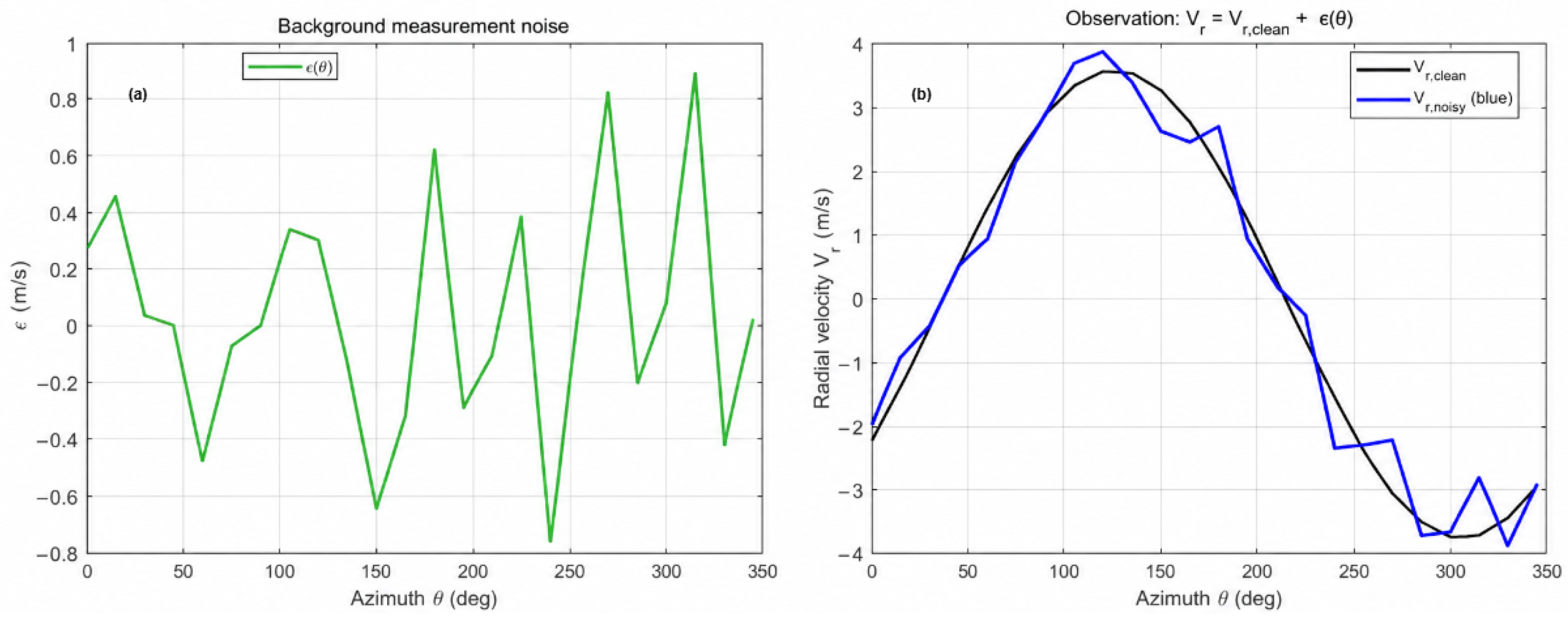
Here, ${\sigma }_{\epsilon }$ characterizes the combined effects of systematic measurement errors and small-scale turbulence fluctuations under the current observational conditions. Based on the radial wind retrieval accuracy of typical Doppler lidar systems operating under moderate signal-to-noise ratio conditions [21], this study selects ${\sigma }_{\epsilon }=0.4\mathrm{m}/\mathrm{s}$ ensuring that the background error is “significantly lower than the wind speed itself but sufficient to influence the retrieval accuracy,” thereby neither obscuring the true wind field structure nor undermining the algorithm’s sensitivity to noise [22,23]. The Figure 5 compares the noise-free radial velocity $V_{r,\mathrm{clean}}$ with the corresponding noisy observation obtained by superimposing additive noise, denoted as $V_{r,\mathrm{noisy}}$.

4.1.3. Construction of Strong Anomalous Observations

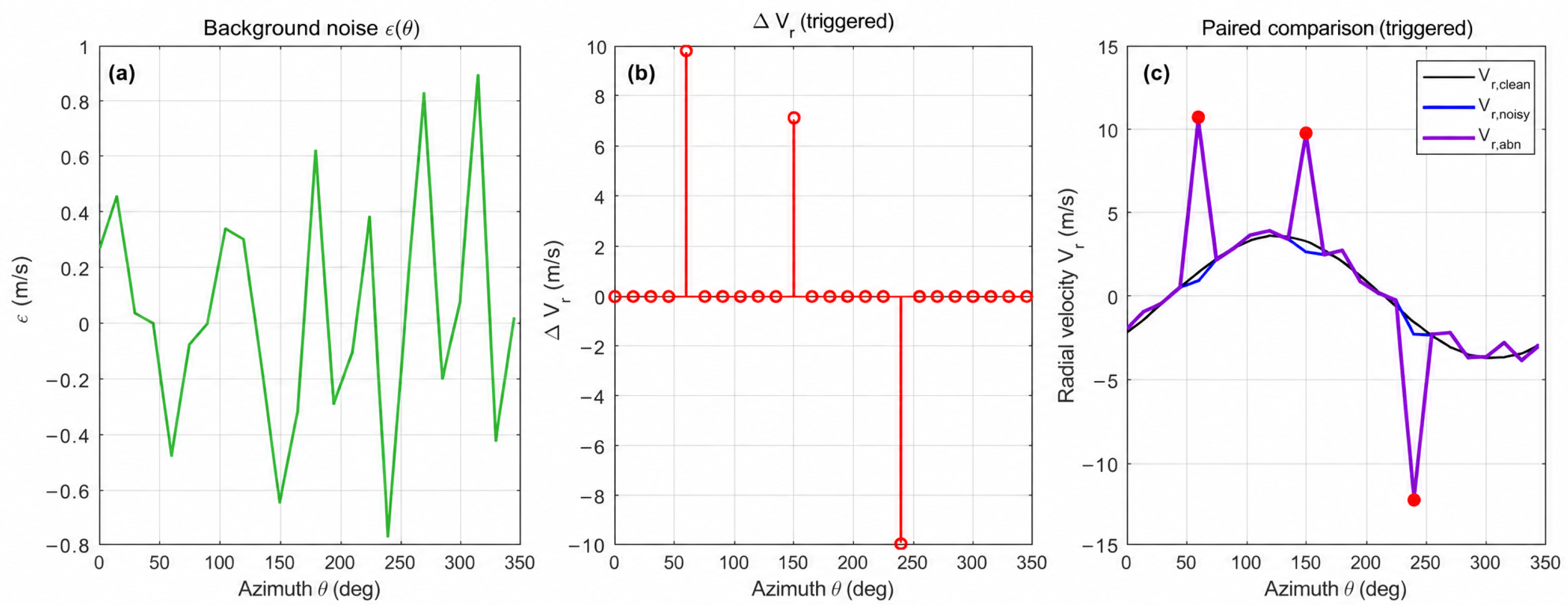
To deliberately investigate the algorithm’s capability to suppress a small number of high-amplitude anomalous points, we further introduce a few extreme anomalous radial wind observations with magnitudes significantly greater than the background Gaussian noise. Specifically, for each observation group consisting of $n_{\mathrm{angle}}$ azimuth angles, a probability of $p_{\mathrm{strong}}=0.25$ is used to determine whether the group contains strong anomalies. If an anomaly is identified, $n_{\mathrm{abn}}$ random azimuth directions are selected as anomalous directions, where $n_{\mathrm{abn}}\in \{1,2,3\}$. For each anomalous direction k, high-amplitude disturbances are added to the original noisy observation $V_{r,\mathrm{noisy}}(i,k)$ as follows: $V_r(i,k)\sim \mathcal{N}({\mu }_{\mathrm{abn}},{\sigma }_{\mathrm{abn}}^2)$, with ${\mu }_{\mathrm{abn}}=10\mathrm{m}/\mathrm{s}$ and ${\sigma }_{\mathrm{abn}}=4\mathrm{m}/\mathrm{s}$, with the sign chosen randomly with a probability of 0.5. Thus, the final anomalous observation is calculated as

$$V_{r,\mathrm{abn}}(i,k)=\left\{\begin{array}{cc}{V}_{r,\mathrm{noisy}}(i,k)+\Delta V_r,\hfill & \mathrm{with}\mathrm{probability}0.5,\hfill \\ V_{r,\mathrm{noisy}}(i,k)-\Delta V_r,\hfill & \mathrm{with}\mathrm{probability}0.5.\hfill \end{array}\right.$$

(37)

The azimuth directions not marked as anomalous remain unchanged

$$V_{r,\mathrm{abn}}(i,k)=V_{r,\mathrm{noisy}}(i,k).$$

(38)

Here, ${\mu }_{\mathrm{abn}}$ and ${\sigma }_{\mathrm{abn}}$ are chosen to be several tens of times the standard deviation of the background noise ${\sigma }_{\epsilon }$, ensuring the amplitudes of the anomalous points are significantly greater than the conventional measurement errors. These anomalous observations can represent extreme values arising from strong clutter echoes, short-term external disturbances, or retrieval failures. By randomizing the anomalous directions, the number of anomalies, and the signs of disturbances, we can statistically cover various possible distributions of anomalies.

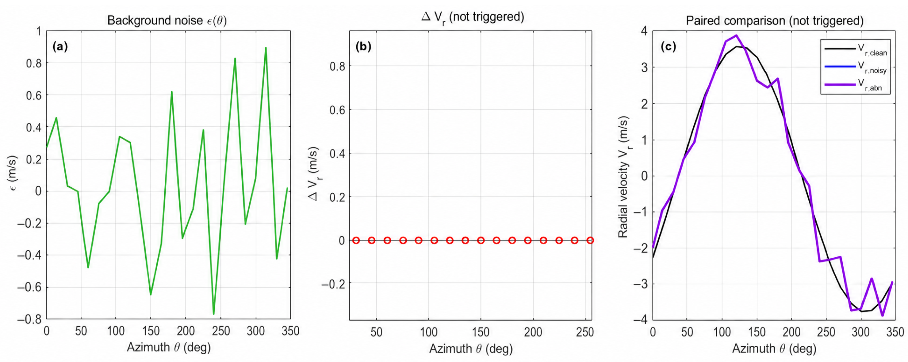
The Figure 6 presents the control case without strong-outlier injection, where $\Delta V_r=0$; consequently, $V_{r,\mathrm{abn}}$ coincides with $V_{r,\mathrm{noisy}}$ and serves as a baseline observation containing background noise only. Correspondingly, Figure 7 also shows an example with strong-outlier injection: the sparse term $\Delta V_r$ acts on only a few azimuths, thereby introducing high-magnitude deviations at those azimuths and yielding $V_{r,\mathrm{abn}}$ contaminated by strong outliers.

In summary, the radial wind observations $V_{r,\mathrm{abn}}$ simulated in this study contain both the small- to medium-amplitude measurement uncertainties represented by the Gaussian noise $\epsilon (i,k)$ and a small number of high-amplitude, randomly distributed outliers represented by $\Delta V_r(i,k)$. This error model can be seen as a classic combination of “observations contaminated by Gaussian noise + low-probability gross errors,” aligning with empirical findings in Doppler lidar observations that “the vast majority of radial wind errors are approximately Gaussian, with a few outliers caused by factors such as clutter.” Meanwhile, all key parameters in the model can be explicitly controlled, enabling a systematic evaluation of the robustness of the KSR-Huber method and comparative algorithms under different noise levels and anomaly strengths, while also supporting a repeatable testing framework for quantitative comparison of anomaly suppression performance. It should be noted that the current anomaly model primarily captures gross-error contamination but does not represent all error mechanisms present in operational CDWL lidar observations, such as azimuthally coherent biases, low-SNR spectral broadening, ground clutter, cloud contamination, and non-uniform aerosol distributions.

The proposed experimental platform characterizes two error sources in actual Doppler lidar observations: (i) small-to-medium random errors caused by measurement noise and small-scale turbulence [24], and (ii) a few high-amplitude anomalous observations potentially associated with ground echo, side-lobe clutter, and short-term disturbances [25]. Compared with full physical simulations, the statistical error model in this study provides explicit control over error magnitude and anomaly ratio, facilitating systematic analyses of algorithm responses under different anomalous scenarios. The experimental setup further corresponds to a typical case where a single Doppler lidar scans a fixed-height layer.

4.1.4. Hyperparameter Selection

To systematically assess the effectiveness of the proposed KSR-Huber method, we quantitatively evaluate its performance against baseline methods under different observational redundancies and anomaly levels using the constructed numerical experimental platform. This controllable environment avoids the interference of uncontrolled factors present in real observations, enhancing the reproducibility of the conclusions.

The hyperparameter selection involves two steps: initial empirical estimation and subsequent fine-tuning via grid search, with all parameter configurations detailed in

Table 1. Hyperparameter settings in KSR-Huber.

Hyperparameter	Initial Value	Final Value
$K_{neighbor}$	4	5
$\alpha$	0.5	0.7
${\sigma }_a$	0.5	0.3
${\sigma }_b$	1.2	1.2
${\delta }_{Huber}$	1.3	1.3

. Initially, configurations were determined based on physical magnitudes and empirical bounds. Specifically, the initial values of $K_{neighbor}$ and $\alpha$ were selected based on recommendations from the KNN-COOKS method in similar radar scenarios, striking a balance between maintaining sensitivity to local anomalies and avoiding overfitting to isolated points. The Sigmoid parameters (${\sigma }_a$ and ${\sigma }_b$) were set according to the empirical distribution of anomaly scores, ensuring a moderate slope. The Huber threshold (${\delta }_{Huber}$) was set to approximately 3 to 4 times the standard deviation of the background noise, providing a robust compromise between Gaussian noise and significant outliers.

Subsequently, to reduce the subjectivity of empirical parameterization, we conducted limited grid searches and sensitivity analyses under formal experimental noise settings. As shown in Table 1, the final parameter combination achieved optimal or near-optimal performance in terms of 3D RMSE and radial wind $R^2$. Importantly, the performance discrepancies observed between the initial parameter set and the fine-tuned final parameters were marginal (less than a few percent). This demonstrates that KSR-Huber is highly insensitive to minor perturbations in hyperparameters within the investigated range, exhibiting excellent parameter robustness.

4.1.5. Sensitivity Analysis of Hyperparameters

To further evaluate the robustness of the selected hyperparameters, we conduct a sensitivity analysis for the key parameters $K_{neighbor}$ and $\alpha$, which control the neighborhood size and the strength of prior weighting, respectively. The parameter $K_{neighbor}$ is varied from 3 to 20, while $\alpha$ ranges from 0.3 to 2. These ranges are chosen to cover typical values used in practice.

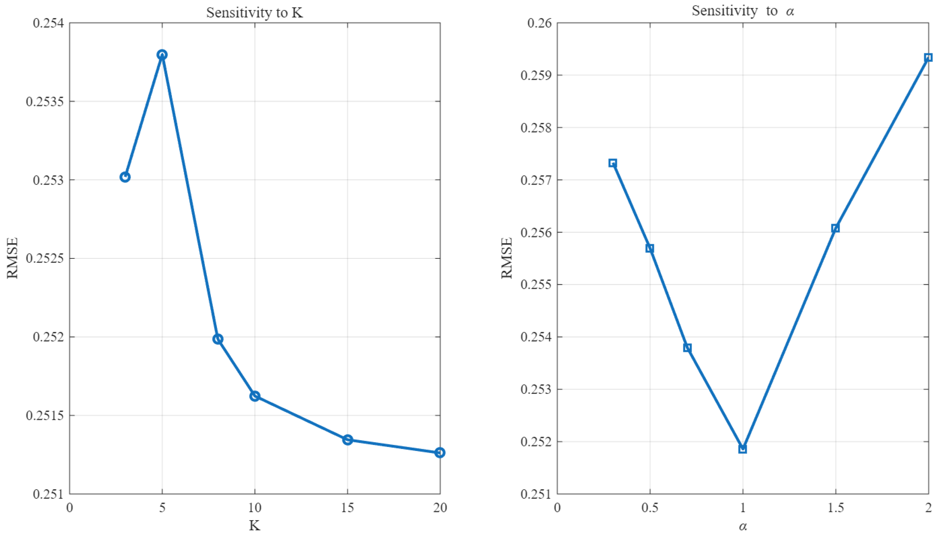
As illustrated in Figure 8, the RMSE varies smoothly with both parameters under a fixed experimental setup. The results are obtained with a fixed random seed to ensure reproducibility. As $K_{neighbor}$ increases, the performance improves initially and then gradually stabilizes, indicating diminishing returns beyond a moderate neighborhood size. This suggests that incorporating local statistical information is beneficial, while the method is not overly sensitive to the precise choice of $K_{neighbor}$. For $\alpha$, a shallow minimum is observed around $\alpha =1$, and the overall variation remains within a narrow range. This indicates that the method maintains stable performance across a relatively broad interval of $\alpha$, without requiring fine-tuning.

The remaining parameters, ${\sigma }_a$, ${\sigma }_b$, and ${\delta }_{Huber}$, are not treated as primary tuning variables. ${\sigma }_a$ and ${\sigma }_b$ control the smoothness of the sigmoid weighting function and are set to ensure stable and monotonic transitions of the weighting function, rather than being tuned to optimize performance for a specific dataset, while ${\delta }_{Huber}$ follows standard practice in robust regression.

Additional tests indicate that moderate variations in these parameters lead to negligible changes in RMSE (on the order of ${10}^{-3}$) and do not affect the overall trends. Therefore, they are fixed to typical values, and the analysis focuses on $K_{neighbor}$ and $\alpha$, which have a more direct impact on performance.Overall, the results indicate that the proposed method maintains stable performance across a broad range of parameter settings.

4.2. Algorithm Performance

4.2.1. Evaluation Metrics

To comprehensively evaluate the algorithm performance, we employ metrics in both the three-dimensional wind vector space and the radial observation space. Let the true three-dimensional wind vector and its retrieved estimate for the i-th sample be ${\mathbf{v}}_i={(u_i,v_i,w_i)}^T$ and ${\widehat{\mathbf{v}}}_i={({\widehat{u}}_i,{\widehat{v}}_i,{\widehat{w}}_i)}^T$, respectively. The retrieval error vector is defined as ${\mathbf{e}}_i={\widehat{\mathbf{v}}}_i-{\mathbf{v}}_i$. To quantify the overall statistical accuracy across $n_{Group}$ trials, the three-dimensional Root Mean Square Error (3D RMSE) and Mean Absolute Error (3D MAE) are calculated as

$${\mathrm{RMSE}}_{3D}=\sqrt{{\displaystyle \frac{1}{n_{Group}}}\sum _{i=1}^{n_{Group}}{\parallel {\mathbf{e}}_i\parallel }_2^2}$$

(39)

$${\mathrm{MAE}}_{3D}={\displaystyle \frac{1}{n_{Group}}}{\displaystyle \sum _{i=1}^{n_{Group}}}{\displaystyle \frac{\parallel {\mathbf{e}}_i{\parallel }_1}{3}}$$

(40)

where ${\parallel ·\parallel }_2$ and ${\parallel ·\parallel }_1$ denote the Euclidean and Manhattan norms, respectively. Additionally, the scalar 3D Euclidean error for a single retrieval is denoted as ${ϵ}_{3D,i}={\parallel {\mathbf{e}}_i\parallel }_2$, which characterizes the absolute distance between the estimated and true wind vectors.

Furthermore, to quantitatively assess how well the retrieved wind field explains the variance of the underlying clean radial velocities, the coefficient of determination ($R^2$) is evaluated in the observation space

$$R^2=1-{\displaystyle \frac{{\sum }_{j=1}^N{\left(v_{r,j}^{clean}-{\widehat{v}}_{r,j}\right)}^2}{{\sum }_{j=1}^N{\left(v_{r,j}^{clean}-{\overline{v}}_r^{clean}\right)}^2}}$$

(41)

where N is the total number of evaluated radial-velocity samples, $v_{r,j}^{clean}$ is the noise-free radial velocity reference, ${\widehat{v}}_{r,j}$ is the back-projected radial velocity calculated from the retrieved 3D wind vector, and ${\overline{v}}_r^{clean}$ is the sample mean of the clean references. An $R^2$ value closer to 1 indicates that the retrieved wind vector accurately reproduces the true radial-velocity variability, whereas a value near or below 0 implies poor model fit.

4.2.2. Simulation Experiment Analysis

Under the simulation setting described above, this section conducts a comparative evaluation of four three-dimensional wind-field retrieval methods (DSWF, KNN-COOKS, airSWF, and the proposed KSR-Huber) in the presence of severe contamination by anomalous radial observations.

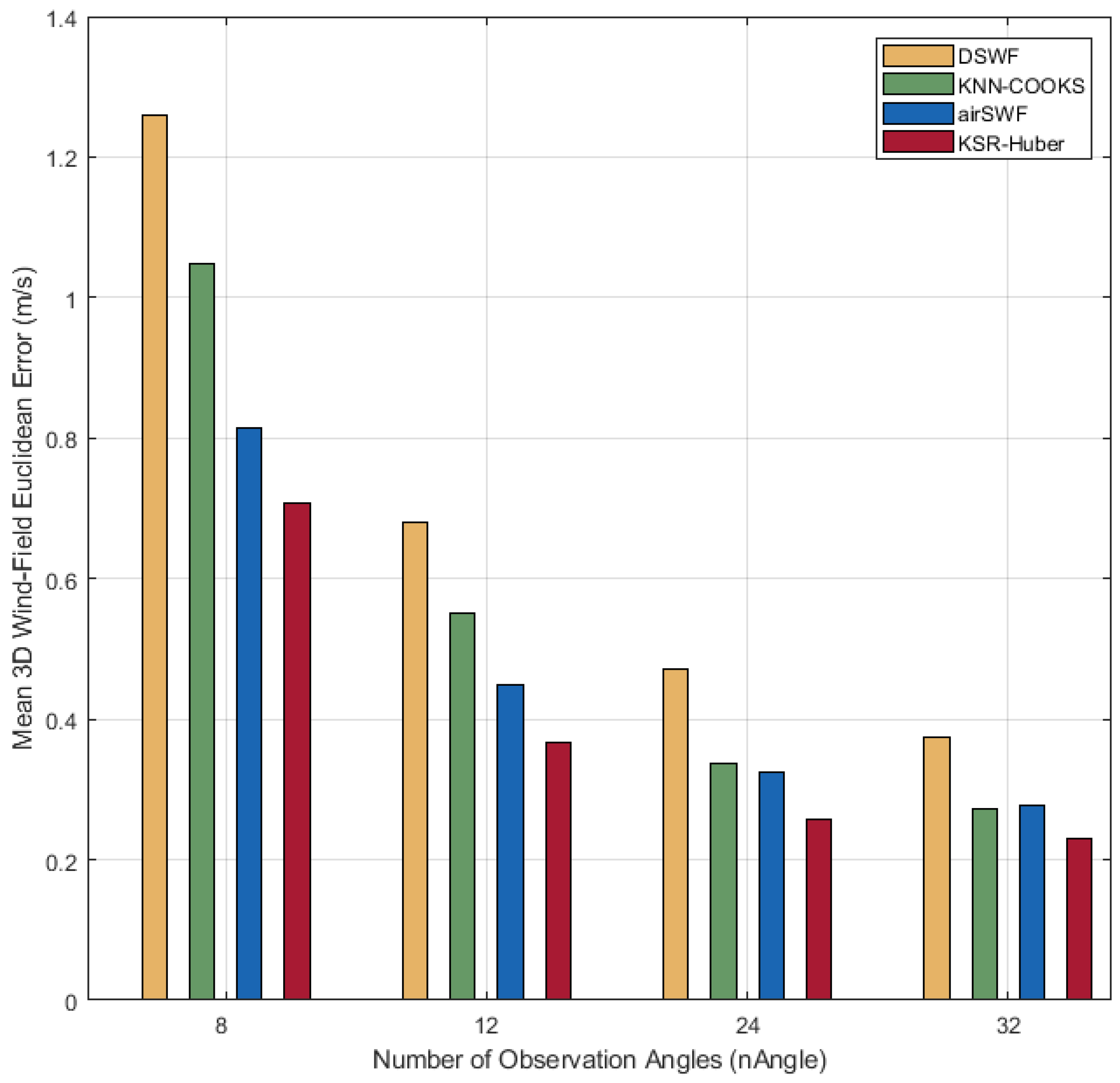
3D Accuracy under Sparse-to-Dense Sampling: As shown in Figure 9, in the most underdetermined setting ($nAngle=\mathbf{8}$), the performance gap is largest. DSWF produces the highest 3D Euclidean error ($1.26\mathrm{m}/\mathrm{s}$), while KNN-COOKS and airSWF reduce it to $1.05\mathrm{m}/\mathrm{s}$ and $0.82\mathrm{m}/\mathrm{s}$, respectively; KSR-Huber further lowers the error to $0.71\mathrm{m}/\mathrm{s}$. Compared with DSWF, KSR-Huber achieves an error reduction of $43.7\%$; relative to KNN-COOKS, it yields an additional reduction of $32.4\%$, and improves upon airSWF by $13.4\%$. When $nAngle$ increases to 12, 24, and 32, the errors of all methods decrease monotonically, with KSR-Huber attaining $0.37\mathrm{m}/\mathrm{s}$, $0.26\mathrm{m}/\mathrm{s}$, and $0.23\mathrm{m}/\mathrm{s}$, respectively. Overall, these results confirm that KSR-Huber is not only more robust to outliers under highly underdetermined observations, but also preserves a consistent performance advantage as redundancy increases.

RMSE and MAE for four retrieval methods across different observation-angle counts ($nAngle$) are reported in

Table 2. Retrieval error metrics of four methods under different numbers of observation angles ($nAngle$).

Method	nAngle = 8		nAngle = 12		nAngle = 24		nAngle = 32
	RMSE	MAE	RMSE	MAE	RMSE	MAE	RMSE	MAE
DSWF	2.187	1.259	1.293	0.680	0.705	0.471	0.531	0.375
KNN-COOKS	1.895	1.048	1.023	0.552	0.433	0.325	0.334	0.272
airSWF	1.457	0.816	0.559	0.449	0.359	0.325	0.304	0.277
KSR-Huber	1.235	0.707	0.434	0.366	0.281	0.258	0.250	0.231

. Overall, errors decrease monotonically as $nAngle$ increases, and KSR-Huber consistently attains the lowest RMSE and MAE. For sparse observations ($nAngle=8$), it achieves RMSE/MAE of 1.235/0.707, outperforming airSWF (1.457/0.816), KNN-COOKS (1.895/1.048), and DSWF (2.187/1.259). At $nAngle=32$, KSR-Huber further reduces RMSE/MAE to 0.250/0.231 while remaining best. Its RMSE and MAE decrease approximately monotonically with only minor variation. Collectively, these results confirm KSR-Huber’s superior absolute accuracy across all observation sparsity regimes.

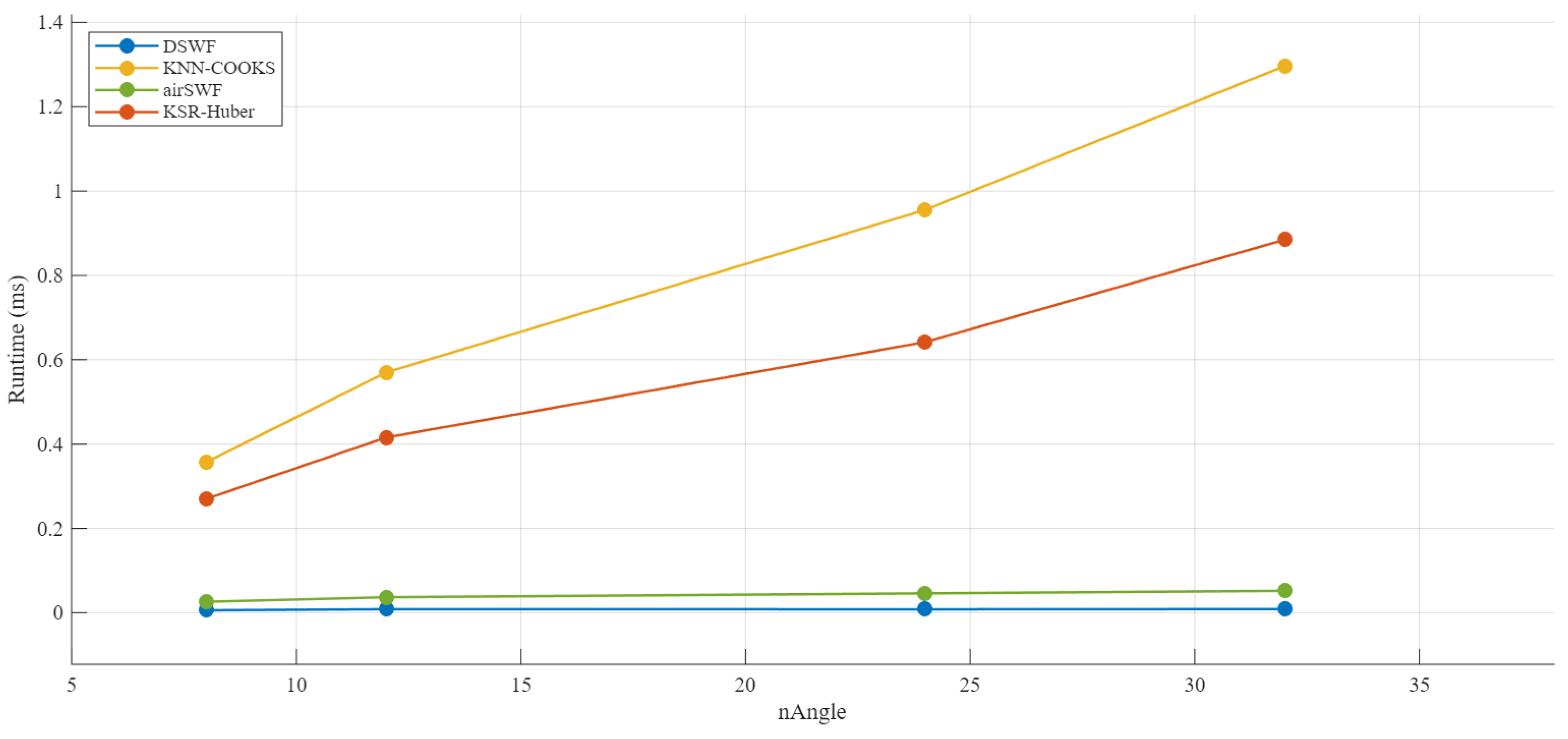
Computational Cost and Scalability: As shown in Figure 10, DSWF and airSWF maintain low and nearly stable runtimes, whereas KNN-COOKS increases notably with nAngle. In contrast, our KSR-Huber exhibits a moderate and controlled runtime growth, indicating that the proposed refinement remains computationally feasible under denser angular sampling.

Table 3. Runtime and IRLS iterations for different $n_{Angle}$.

${\mathit{n}}_{\mathit{Angle}}$	Runtime (ms)				IRLS Iterations (Mean)
	DSWF	KNN-COOKS	airSWF	KSR-Huber
8	0.00601	0.37575	0.02597	0.27027	5.36
12	0.00859	0.56970	0.03994	0.41578	4.66
24	0.00803	0.95597	0.04595	0.64182	4.06
32	0.00845	1.29622	0.05195	0.88444	4.05

further reports that the average IRLS iteration number decreases from $5.36$ ($n_{Angle}=8$) to about $4.05$ ($n_{Angle}=32$), suggesting that the refinement overhead does not increase with denser angular sampling and is consistent with the runtime trend in Figure 10.

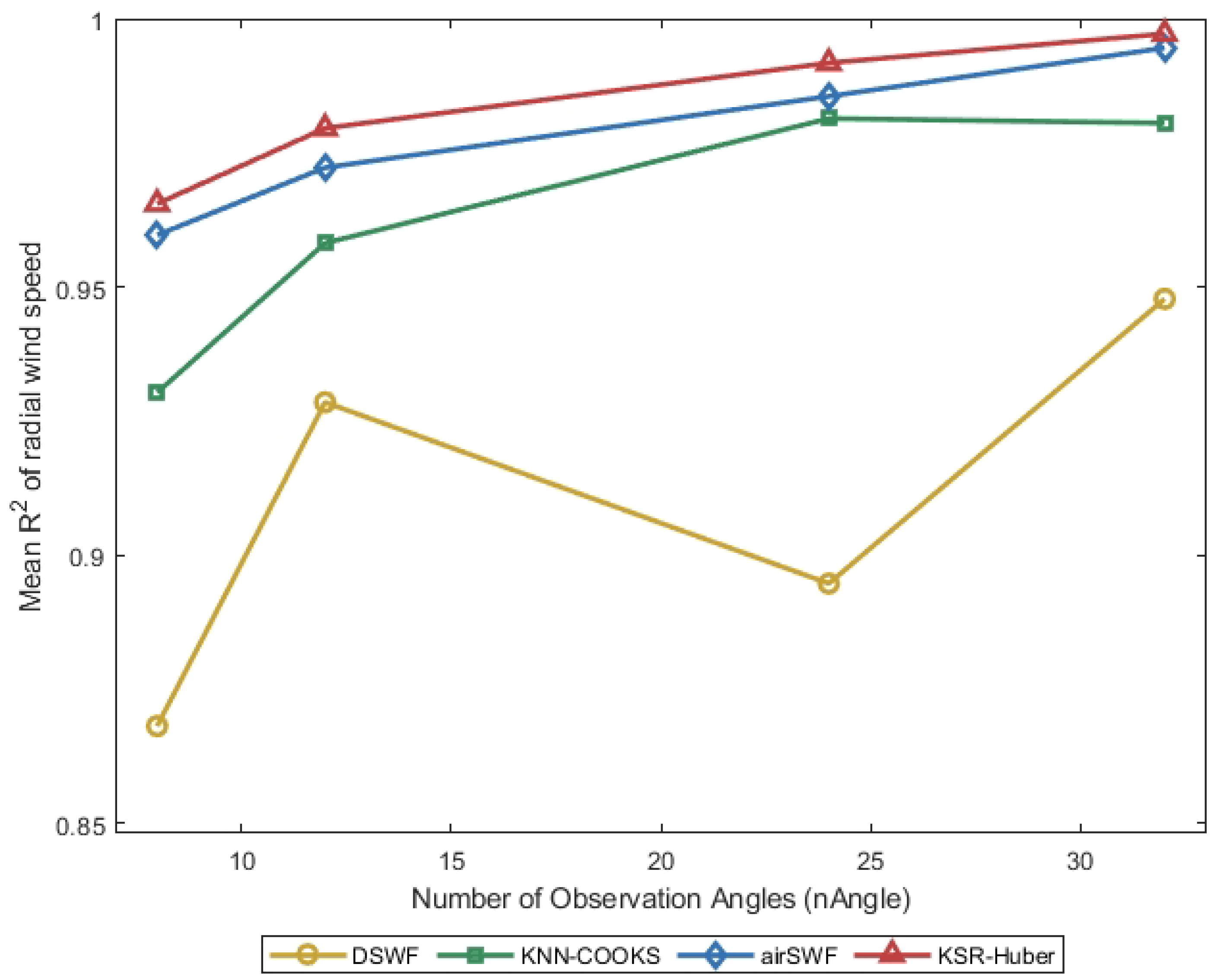
Radial-velocity fit consistency via $R^2$: We further compare the radial-velocity goodness of fit ($R^2$) of the four retrieval methods under different numbers of observation angles ($nAngle$). As illustrated in Figure 11, KSR-Huber exhibits a smoother overall curve and consistently achieves the highest $R^2$ across all $nAngle$ settings, indicating superior fitting accuracy and more stable performance. In contrast, the $R^2$ values of airSWF and KNN-COOKS are generally lower than those of KSR-Huber. DSWF yields the lowest $R^2$ and displays pronounced fluctuations, suggesting that its least-squares-based sinusoidal fitting is highly sensitive to strong outliers, where even a small number of anomalous observations can introduce substantial bias and degrade the overall fit quality. Overall, these results consistently demonstrate that KSR-Huber outperforms the three baseline methods in terms of fitting accuracy, robustness, and adaptability to sparse observation configurations.

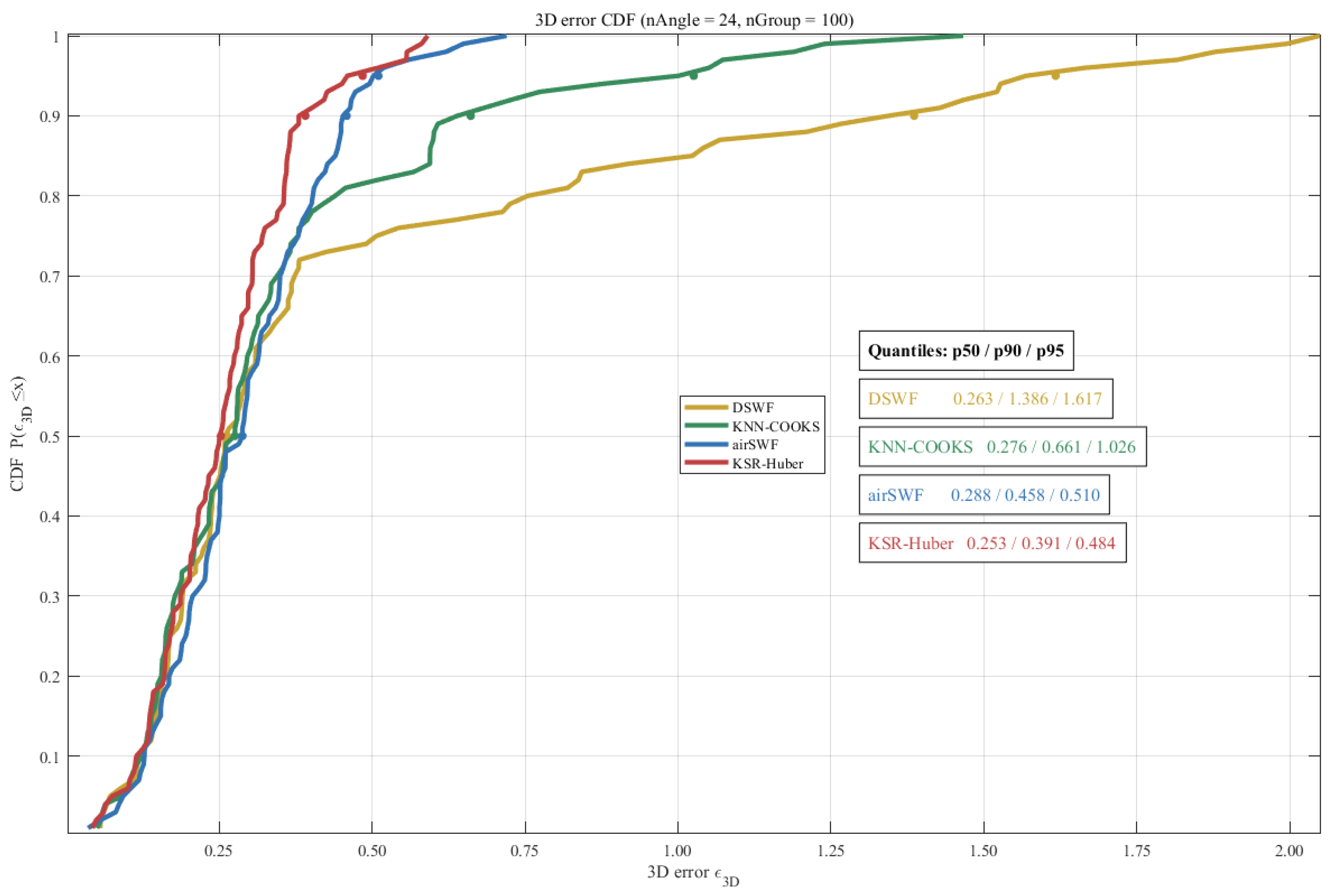
Tail-risk characterization via CDF: The cumulative distribution functions (CDFs) of the three-dimensional wind-vector error ${ϵ}_{3D}={\parallel \widehat{\mathbf{V}}-{\mathbf{V}}_{\mathrm{true}}\parallel }_2$ are presented in Figure 12 for different retrieval methods under $nAngle=24$ and $nGroup=100$. A CDF curve that lies further to the left and rises more steeply indicates that a larger fraction of samples is captured at smaller error thresholds, reflecting higher overall accuracy and robustness. In contrast, a right-shifted curve or an elongated tail suggests more frequent large-error events and, consequently, higher long-tail risk. The $p50/p90/p95$ percentiles are also reported to characterize both the typical error level and tail behavior.

The percentile statistics and the CDF shapes lead to consistent conclusions. KSR-Huber dominates across all percentiles, with $p50$, $p90$, and $p95$ equal to 0.253, 0.391, and 0.484, respectively. It not only achieves the lowest median error but also markedly reduces high-percentile errors, indicating an enhanced ability to suppress error proliferation and to mitigate the occurrence of extreme errors under the coexistence of strong noise and outliers. By comparison, the other three baselines exhibit varying degrees of right shift and heavier tails, implying lower sample coverage at the same error threshold, higher overall error levels, and a greater propensity for large-error events, i.e., weaker tail-risk control. Overall, the collective evidence from the left-shifted CDF, the shorter tail, and the associated percentile metrics demonstrates that KSR-Huber simultaneously attains lower typical errors and stronger suppression of tail risk in this wind-vector retrieval task.

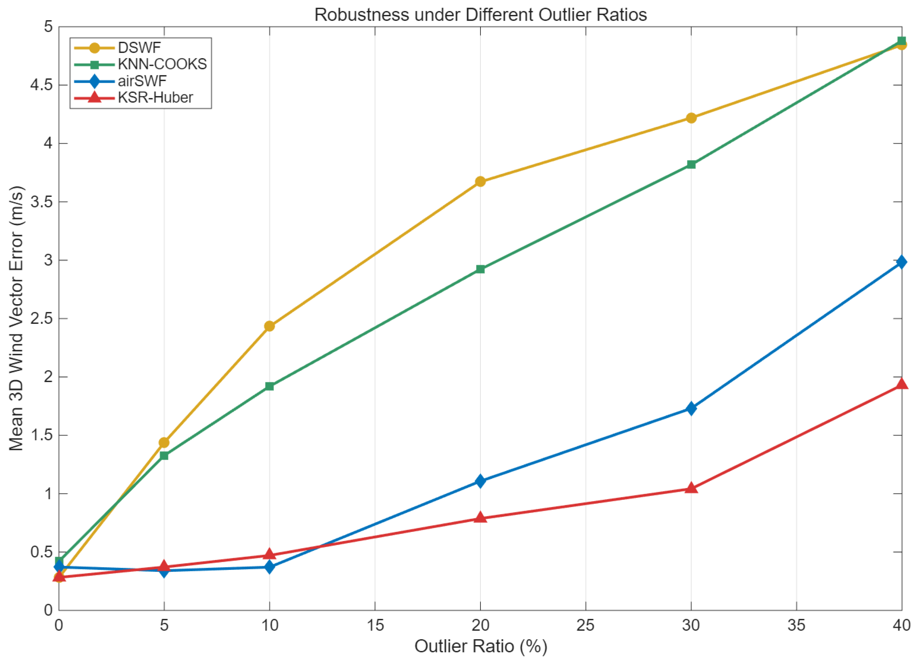
Robustness under strong anomalous observations: To assess the robustness of different wind retrieval methods in the presence of abnormal observations, simulation experiments were conducted with outlier ratios ranging from $0\%$ to $40\%$. Four approaches were evaluated, including DSWF, KNN-COOKS, airSWF, and the proposed KSR-Huber method. The mean three-dimensional wind vector error was adopted as the evaluation metric.

As illustrated in Figure 13, the estimation error of all methods increases with the outlier ratio, while the performance gap between methods becomes progressively more pronounced. The DSWF method is particularly sensitive to abnormal observations. Its error grows rapidly as the outlier ratio increases, reaching nearly $4.8$ m/s at an outlier ratio of $40\%$, which is more than an order of magnitude larger than the error under the outlier-free condition. KNN-COOKS and airSWF improve robustness to some extent; however, their estimation errors still increase considerably when the contamination level becomes high.

In contrast, the proposed KSR-Huber method consistently achieves the lowest estimation error across most outlier ratios. At an outlier ratio of $40\%$, the error of the proposed method is approximately $1.9$ m/s, representing a reduction of about $60\%$ compared with both DSWF and KNN-COOKS, and about $35\%$ compared with airSWF. Moreover, when the outlier ratio increases from $0\%$ to $40\%$, the error of the proposed method increases only from approximately $0.3$ m/s to $1.9$ m/s, which is substantially smaller than the degradation observed for the other methods.

These results show that the proposed KNN-based structural weighting combined with the Huber estimator suppresses abnormal observations and significantly improves the robustness of wind-field reconstruction under highly contaminated measurements.

4.3. Robustness Analysis Under Different Noise Levels

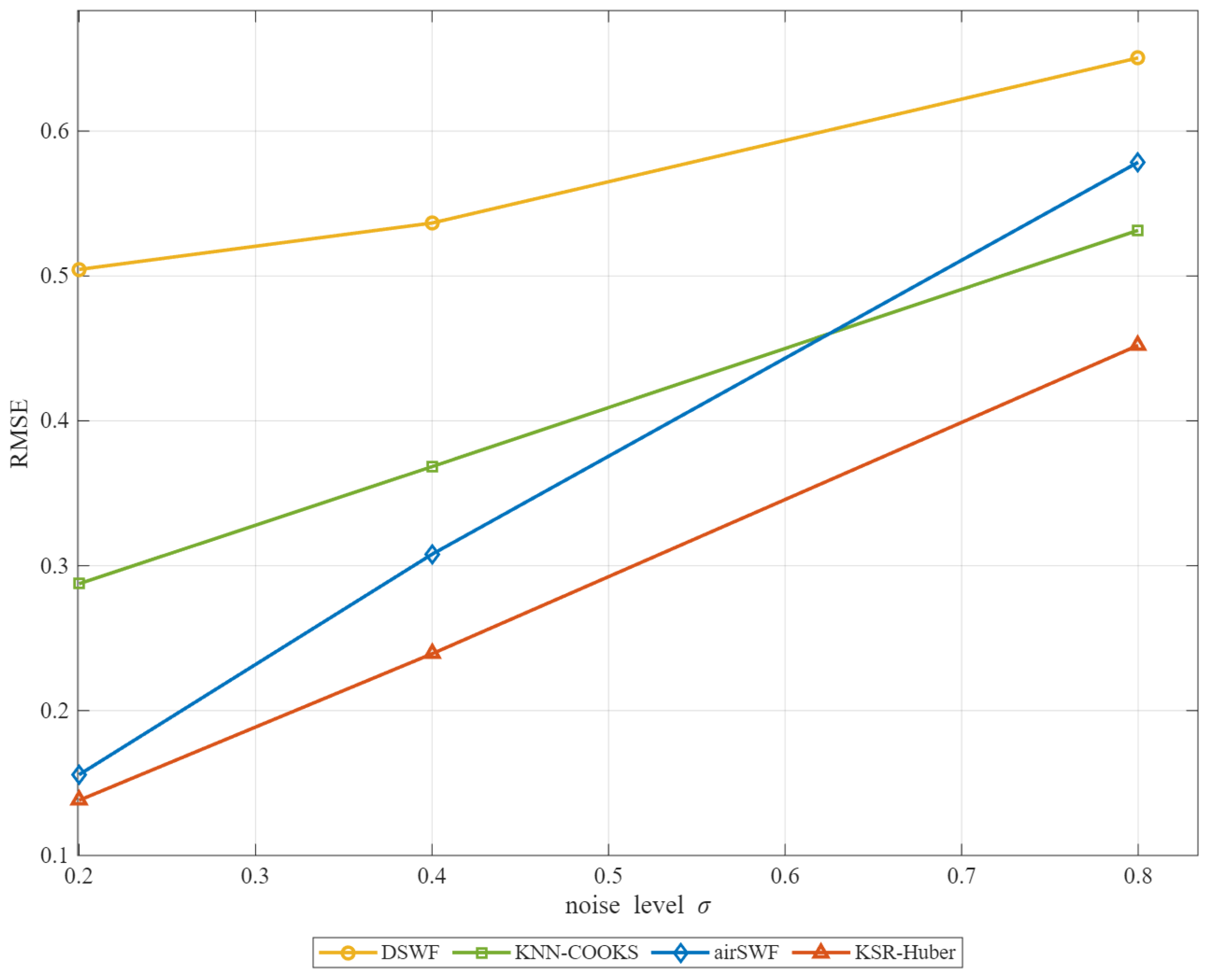
To further evaluate the robustness of the proposed method, additional experiments were conducted under different noise levels. Gaussian noise with standard deviations $\sigma =0.2,0.4,0.8$ was added to the simulated radial velocity measurements. Each experiment was repeated five times, and the averaged RMSE values were reported to ensure statistical stability.

As shown in Figure 14, the RMSE of all methods increases with the noise level. However, the proposed KSR-Huber method consistently achieves the lowest RMSE across all noise levels, demonstrating its superior robustness under varying noise conditions. This advantage remains evident even in the presence of strong noise and outliers.

4.4. Algorithm Comparison Based on Real Data

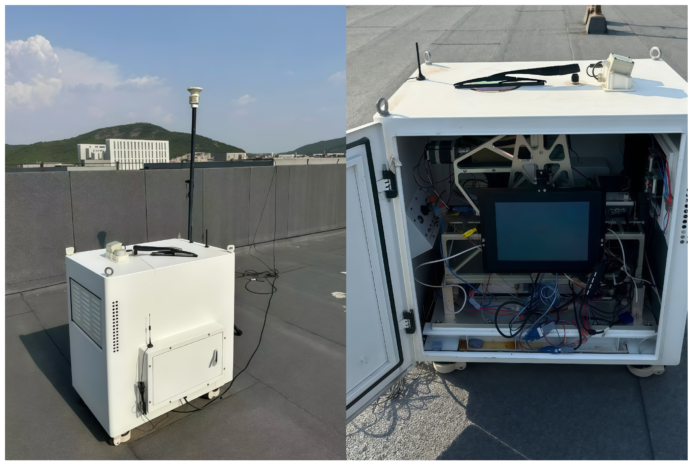
To evaluate the effectiveness of the proposed KSR-Huber method in practical applications, a field experiment was conducted on 22–23 April 2026 using a coherent Doppler wind lidar (CDWL) system at Shandong Normal University, Changqing District, Jinan, Shandong Province, China (36.5°N, 116.8°E). A schematic diagram of the CDWL system is presented in Figure 15.

Table 4. Pooled peak statistics across azimuths.

Epoch	$\mathbf{Peak}\text{\_}\mathbf{Count}$: Median (IQR)	$\mathbf{Peak}\text{\_}\mathbf{Height}$: Median (IQR)
22 April 2026	30.5000 (2.0000)	2.9436 (0.3204)
23 April 2026	34.0000 (2.5000)	3.7668 (0.2947)

summarizes pooled peak statistics across two observation dates (22 April 2026 and 23 April 2026). The pooled statistics report two characterization metrics, peak_count (median (IQR)) and peak_height (median (IQR)), which quantify the peak occurrence frequency and peak strength in each day’s observations. Overall, these metrics show variations in the peak-statistical characteristics between the two dates, which may be associated with changes in the corresponding atmospheric conditions. Moreover, the wind-field conditions are not the same across the two observation days.

In this study, we use a CDWL system manufactured by Hefei Technovo Lidar Hi-Tech Co., Ltd. in Hefei, China (model KC-WL-2006 Lidar). Operating at a wavelength of 1550 nm with a center frequency of 80 MHz, the instrument utilizes a 1 GHz sampling rate to achieve a spatial range resolution of 60 m. It is capable of effective detection up to a distance of 3000 m, covering a wind speed measurement range of 62 m/s. To retrieve the horizontal wind fields during scanning operations, the classical velocity azimuth display (VAD) technique is employed. The main parameters of the coherent Doppler wind lidar system are shown in

Table 5. System parameters of the coherent Doppler wind lidar.

Transmitter		Transceiver		Data Acquisition
Wavelength	1550 nm	Laser mode	Pulse	Sampling frequency	1 GHz
Pulse energy	145 $\mathsf{\mu }$J	Scan mode	Conical	Sampling points	400
Pulse repetition	10 KHz	Elevation angle	${60}^{\circ }$	Range resolution	60 m
Pulse width	400 ns	Step angle	${90}^{\circ }$	Gate number	128

.

The experimental data were acquired using a multi-beam scanning configuration. Specifically, observations were conducted at four azimuth angles (0°, 90°, 180°, and 270°), resulting in two sets of radial velocity measurements and covering 40 range gates (height levels). During the measurement process, atmospheric backscattered signals were received by the lidar system and sampled through the data acquisition module. The continuous time-domain signals were subsequently segmented into discrete range gates according to the propagation distance. Spectral estimation was then performed to obtain the Doppler power spectrum, from which the Doppler frequency shift was extracted. Based on the retrieved radial velocities from multiple beam directions, the three-dimensional wind field was reconstructed using different inversion methods.

To assess the proposed KSR-Huber method under real-world conditions, we compared it against established baselines—DSWF, KNN-COOKS, and airSWF—using radial velocity data from the field experiment.

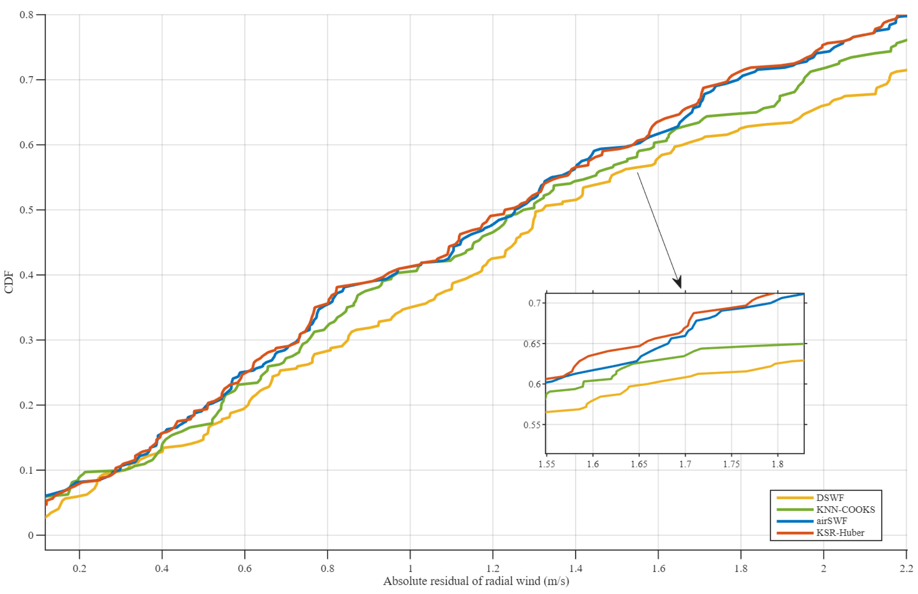
As shown in Figure 16, the residual distributions obtained by all methods are from the 22 April 2026 observational data over the same height interval and exhibit strong overall agreement. The residual is defined as the absolute difference in radial wind, $\left|r\right|=|V_{r,\mathrm{obs}}-V_{r,\mathrm{fit}}|$, and the corresponding CDFs increase monotonically as the threshold $\left|r\right|$ grows, indicating that each method yields satisfactory fits for the majority of samples. However, meaningful discrimination persists in the critical range of small-to-moderate residuals, and the separation is most pronounced in the upper tail. Quantitatively,

Table 6. Statistics of the absolute radial-wind residuals across methods, including the median $\left|r\right|$, $p_{95}$, and the tail probability $P\left(\right|r|>2.5\mathrm{m}/\mathrm{s})$.

Method	$\mathit{median}\text{\_}\mathit{r}$	$\mathit{p}95\text{\_}\mathit{r}$	$\mathit{P}\left(\right|\mathit{r}|>2.5)$
DSWF	1.3241	4.0408	0.2188
KNN-COOKS	1.2865	3.5675	0.1875
airSWF	1.2584	3.4542	0.1781
KSR-Huber	1.2404	3.4137	0.1719

summarizes the median residual, $p_{95}$, and the tail probability $P\left(\right|r|>2.5\mathrm{m}/\mathrm{s})$. KSR-Huber delivers the best overall performance: it achieves the smallest median $\left|r\right|$ (1.2404), the lowest $p_{95}$ (3.4137), and the minimum tail probability (0.1719), demonstrating superior robustness to extreme residual realizations. By contrast, DSWF results in larger median residuals and $p_{95}$ values, together with the largest $P\left(\right|r|>2.5\mathrm{m}/\mathrm{s})$, implying more substantial inconsistencies in the tail region. KNN-COOKS and airSWF occupy an intermediate position between these two extremes. Overall, the concordance between the residual CDFs and the tail statistics confirms that KSR-Huber more effectively reduces the magnitude of retrieval errors while mitigating tail risk under realistic observational conditions, thereby further substantiating its effectiveness and stability for real data.

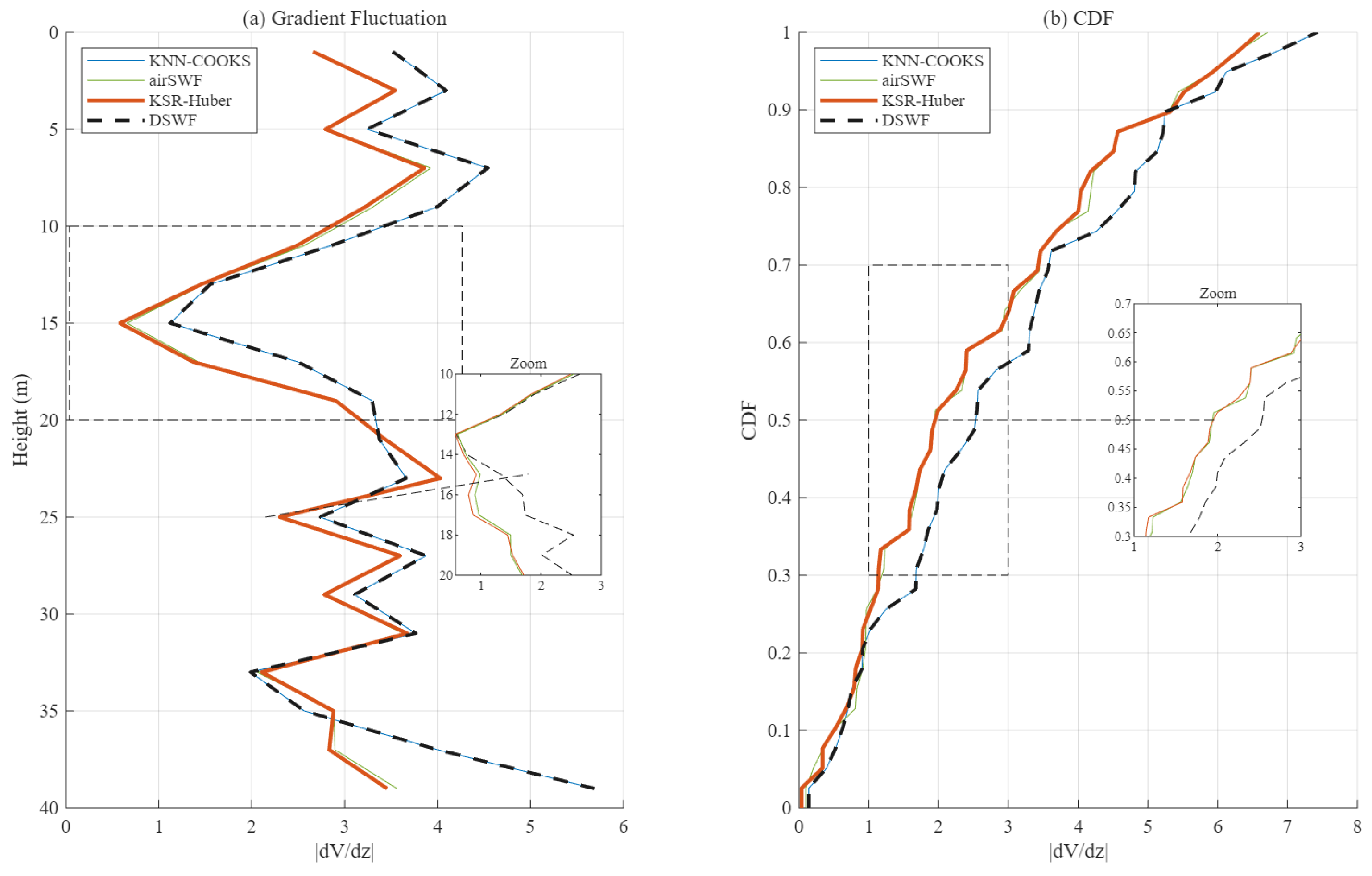
As shown in Figure 17a, the vertical profiles of wind field gradient fluctuation ($\left|{\displaystyle \frac{dV}{dz}}\right|$) indicate that all methods capture height-dependent structural variations in a broadly consistent manner. Differences become more pronounced in zones of intense fluctuation, such as the 10–20 m range. In these regions, KSR-Huber appears to produce a smoother and more consistent gradient profile, reducing anomalous oscillations while preserving the main trends (as highlighted in the zoomed inset, where continuity is maintained without clear evidence of excessive smoothing). By comparison, KNN-COOKS and airSWF exhibit greater local variability, suggesting higher sensitivity to noise, whereas DSWF shows relatively less stable behavior in the same intervals.

Figure 17b further complements this analysis by illustrating the CDFs of gradient magnitudes, providing additional insight into distributional robustness. The KSR-Huber curve tends to increase more steeply and remain more compact overall, consistent with reduced variability and outlier suppression. This tendency is also reflected in the magnified section, where tighter clustering relative to the baselines can be observed. These real-data indicators are consistent with the simulation observations in Section 4.2 (including lower RMSE and higher $R^2$ under noisy scenarios), and they further demonstrate improved stability and distributional agreement.

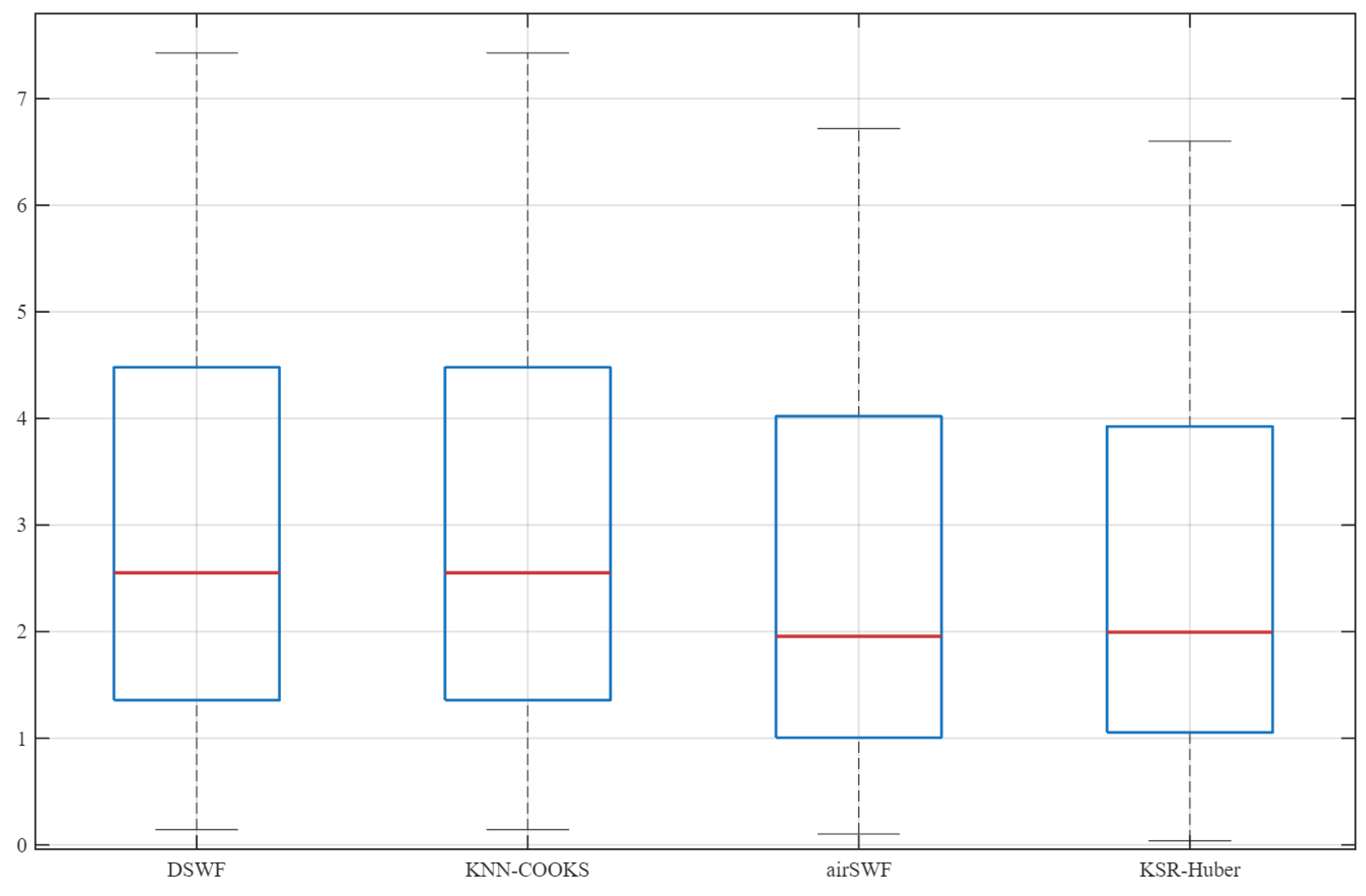
Figure 18 illustrates the distribution of the vertical gradient magnitude ($\left|{\displaystyle \frac{dV}{dz}}\right|$) for the compared methods. DSWF and KNN-COOKS show higher median values together with wider interquartile ranges, which suggests stronger variability and increased sensitivity to noise. In contrast, airSWF and KSR-Huber yield lower medians and more concentrated distributions, indicating enhanced robustness in terms of gradient estimation behavior.

Notably, KSR-Huber maintains a comparatively narrower interquartile range and shorter whiskers, suggesting a more effective suppression of extreme deviations. Overall, these results provide evidence that the proposed approach can alleviate noise-induced fluctuations while retaining key structural characteristics of the signal. However, since this validation is primarily based on gradient smoothness and distributional comparisons, it should be interpreted as supporting improved stability rather than a definitive demonstration of absolute accuracy. We will expand this investigation in future work, including incorporating independent reference measurements for a more rigorous evaluation.

5. Discussion

The results demonstrate that KSR-Huber consistently improves the accuracy and robustness of VAD wind vector retrieval under challenging observational conditions, including sparse sampling, elevated noise levels, and severe outlier contamination. Compared with conventional least-squares approaches, the proposed framework integrates local statistical information with robust regression to provide reliable wind-field estimates in the presence of measurement uncertainty and gross errors. The performance gain stems from the complementary roles of the KNN-based local statistical prior and the Huber IRLS optimization. Their integration effectively balances noise suppression with information preservation by reducing the influence of abnormal observations while retaining statistically consistent measurements. Beyond the improvement in retrieval performance, the proposed framework provides a general strategy for robust inverse modelling with spatially correlated observations. Although developed for wind vector retrieval, the underlying methodology is readily applicable to a broader class of atmospheric remote sensing retrieval problems characterized by sparse observations, spatial dependence, and non-Gaussian measurement errors.

Despite its promising performance, several limitations should be acknowledged. The current evaluation is primarily based on simulated datasets with controlled noise and outlier characteristics. Although such experiments enable systematic assessment of algorithmic robustness, they cannot fully capture the complexity of real atmospheric environments. In particular, strong spatial non-stationarity, rapidly evolving turbulent structures, and systematic measurement biases may challenge the assumption of local statistical consistency. Future work will therefore focus on validation against independent field observations, including collocated Doppler lidars, meteorological towers, and radiosonde measurements acquired under diverse atmospheric stability regimes and complex terrain. Such validation will provide a more comprehensive assessment of the operational applicability and generalizability of KSR-Huber.

6. Conclusions

This study proposes KSR-Huber, a robust method for retrieving three-dimensional wind vectors from coherent Doppler wind lidar observations in VAD mode. Motivated by the presence of intermittent anomalies in radial velocity caused by low signal-to-noise ratios and other measurement errors, KSR-Huber integrates K-nearest-neighbor (KNN) local statistical priors with Huber iterative reweighted least squares (IRLS). The KNN-based local weighting reduces reliance on hard filtering thresholds by exploiting local statistical consistency, while the adaptive Sigmoid weighting enables continuous reweighting of measurements. The unified formulation mitigates sensitivity to unstable initial least-squares estimates by integrating local consistency with robust residual modeling. Simulation results under controlled noisy and sparse observation conditions show that KSR-Huber achieves improved performance and stability of wind estimates compared to DSWF and airSWF, while effectively mitigating extreme-error cases. These results demonstrate the robustness of the proposed method under controlled synthetic noise and outlier conditions. While the method shows promising potential for wind-field retrieval, comprehensive validation against independent observational references remains for future work.

References

1. Liu, Z.; Barlow, J.F.; Chan, P.W.; Fung, J.C.H.; Li, Y.; Ren, C.; Mak, H.W.L.; Ng, E. A Review of Progress and Applications of Pulsed Doppler Wind LiDARs. Remote Sens. 2019, 11, 2522. [Google Scholar] [CrossRef]
2. Liu, X.; Zhang, H.; Wu, S.; Wang, Q.; He, Z.; Zhang, J.; Li, R.; Liu, S.; Zhang, X. Effects of buildings on wind shear at the airport: Field measurement by coherent Doppler lidar. J. Wind Eng. Ind. Aerodyn. 2022, 230, 105–194. [Google Scholar] [CrossRef]
3. Krishnamurthy, R.; Choukulkar, A.; Calhoun, R.; Fine, J.; Oliver, A.; Barr, K.S. Coherent Doppler lidar for wind farm characterization. Wind Energy 2013, 16, 189–206. [Google Scholar]
4. Luo, Z.; Song, X.; Yin, J.; Bu, Z.; Chen, Y.; Yu, Y.; Zhang, Z. Comparison and Verification of Coherent Doppler Wind Lidar and Radiosonde Data in the Beijing Urban Area. Adv. Atmos. Sci. 2024, 41, 2203–2214. [Google Scholar] [CrossRef]
5. Frehlich, R. Simulation of Coherent Doppler Lidar Performance in the Weak-Signal Regime. J. Atmos. Ocean. Technol. 1996, 13, 646–658. [Google Scholar] [CrossRef]
6. Banakh, V.A.; Smalikho, I.N.; Falits, A.V.; Sherstobitov, A.M. Estimating the Parameters of Wind Turbulence from Spectra of Radial Velocity Measured by a Pulsed Doppler Lidar. Remote Sens. 2021, 13, 2071. [Google Scholar] [CrossRef]
7. Augere, B.; Valla, M.; Durécu, A.; Dolfi-Bouteyre, A.; Goular, D.; Gustave, F.; Planchat, C.; Fleury, D.; Huet, T.; Besson, C. Three-Dimensional Wind Measurements with the Fibered Airborne Coherent Doppler Wind Lidar LIVE. Atmosphere 2019, 10, 549. [Google Scholar] [CrossRef]
8. Smalikho, I. Techniques of Wind Vector Estimation from Data Measured with a Scanning Coherent Doppler Lidar. J. Atmos. Ocean. Technol. 2003, 20, 276–291. [Google Scholar] [CrossRef]
9. Abdelazim, S.; Santoro, D.; Arend, M.; Moshary, F.; Ahmed, S. A Hardware Implemented Autocorrelation Technique for Estimating Power Spectral Density for Processing Signals from a Doppler Wind Lidar System. Sensors 2018, 18, 4170. [Google Scholar] [CrossRef] [PubMed]
10. Rui, X.; Guo, P.; Chen, H.; Chen, S.; Zhang, Y. Adaptive iteratively reweighted sine wave fitting method for rapid wind vector estimation of pulsed coherent Doppler lidar. Opt. Express 2019, 27, 21319–21334. [Google Scholar] [CrossRef] [PubMed]
11. Yu, J.; Guo, P.; Chen, S.; Chen, H.; Cao, R.; Xie, Y.; Zou, Z.; Yin, S.; Yu, Y.; Liu, J.; et al. Wind vector retrieval algorithm for a coherent Doppler lidar based on KNN-COOKS. Appl. Opt. 2025, 64, 2640–2652. [Google Scholar] [CrossRef] [PubMed]
12. Teschke, G.; Lehmann, V. Mean wind vector estimation using the velocity–azimuth display (VAD) method: An explicit algebraic solution. Atmos. Meas. Tech. 2017, 10, 3265–3271. [Google Scholar] [CrossRef]
13. Diao, W.; Zhang, X.; Liu, J.; Zhu, X.; Liu, Y.; Bi, D.; Chen, W. All fiber pulsed coherent lidar development for wind profiles measurements i boundary layers. Chin. Opt. Lett. 2014, 12, 072801. [Google Scholar] [CrossRef]
14. Baidar, S.; Wagner, T.J.; Turner, D.D.; Brewer, W.A. Using optimal estimation to retrieve winds from velocity-azimuth display (VAD) scans by a Doppler lidar. Atmos. Meas. Tech. 2023, 16, 3715–3726. [Google Scholar] [CrossRef]
15. Wang, H.; Barthelmie, R.J.; Clifton, A.; Pryor, S.C. Wind Measurements from Arc Scans with Doppler Wind Lidar. J. Atmos. Ocean. Technol. 2015, 32, 2024–2040. [Google Scholar] [CrossRef]
16. Liou, Y.C. An Explanation of the Wind Speed Underestimation Obtained from a Least Squares Type Single-Doppler Radar Velocity Retrieval Method. J. Appl. Meteorol. 2002, 41, 811–823. [Google Scholar] [CrossRef]
17. Held, D.P.; Mann, J. Comparison of methods to derive radial wind speed from a continuous-wave coherent lidar Doppler spectrum. Atmos. Meas. Tech. 2018, 11, 6339–6350. [Google Scholar] [CrossRef]
18. Kongara, S.; Calhoun, R.; Choukulkar, A.; Boldi, M.O. Velocity retrieval for coherent Doppler lidar. Int. J. Remote Sens. 2012, 33, 3596–3613. [Google Scholar] [CrossRef]
19. Zhao, Y.; Yuan, L.; Fan, C.; Zhu, X.; Liu, J.; Dai, B.; Xiao, W.; Zhu, X.; Chen, W. Wind retrieval for genetic algorithm-based coherent Doppler wind lidar employing airborne platform. Appl. Phys. B 2023, 129, 36. [Google Scholar] [CrossRef]
20. Zhang, Z.M.; Chen, S.; Liang, Y.Z. Baseline correction using adaptive iteratively reweighted penalized least squares. Analyst 2010, 135, 1138–1146. [Google Scholar] [CrossRef] [PubMed]
21. Hooper, D.A. Signal and noise level estimation for narrow spectral width returns observed by the Indian MST radar. Radio Sci. 1999, 34, 859–870. [Google Scholar] [CrossRef]
22. Wissel, L.; Hartwig, O.; Bayle, J.B.; Staab, M.; Fitzsimons, E.D.; Hewitson, M.; Heinzel, G. Influence of Laser Relative-Intensity Noise on the Laser Interferometer Space Antenna. Phys. Rev. Appl. 2023, 20, 014016. [Google Scholar] [CrossRef]
23. Wei, T.; Xia, H.; Wu, Y.; Yuan, J.; Wang, C.; Dou, X. Inversion probability enhancement of all-fiber CDWL by noise modeling and robust fitting. Opt. Express 2020, 28, 29662–29675. [Google Scholar] [CrossRef] [PubMed]
24. Rui, X.; Guo, P.; Chen, H.; Chen, S.; Zhang, Y.; Zhao, M.; Wu, Y.; Zhao, P. Portable coherent Doppler light detection and ranging for boundary-layer wind sensing. Opt. Eng. 2019, 58, 034105. [Google Scholar] [CrossRef]
25. Poette, J.; Besnard, P.; Bramerie, L.; Simon, J.C. Highly sensitive measurement technique of relative intensity noise and laser characterization. Fluct. Noise Lett. 2008, 8, L81–L86. [Google Scholar] [CrossRef]
Figure 1. Doppler Lidar conical scan geometry and wind vector decomposition.
Remotesensing 18 02698 g001
Figure 2. Flowchart of the KSR-Huber algorithm with two stages: KNN-Sigmoid prior reweighting and Huber IRLS refinement. The iteration stops when Δ v < ε .
Remotesensing 18 02698 g002
Figure 3. Stage I: KNN–Sigmoid prior reweighting via local consistency evaluation (KSR): (a) compute local inconsistency D j and scale s j via KNN-based evaluation; (b) fuse global–local features as z j = α D j * + ( 1 α ) x j ; (c) map z j to prior weights through an adaptive KNN–sigmoid module.
Remotesensing 18 02698 g003
Figure 4. Stage II: Huber IRLS Residual Reweighting and Coupled Weighted Least-Squares Updates: (a) residual computation at iteration t and Huber-based reweighting determined by | r j ( t ) | relative to δ Huber ; (b) coupled weighted least-squares update using the combined weights W ( t ) to obtain v ( t + 1 ) . (c) coupled weights construction and wind vector update: W ( t ) = diag ( W j ( t ) ) , w j ( t ) = w ˜ j prior · w j Huber , and v ( t + 1 ) = ( A W ( t ) A ) 1 A W ( t ) V r .
Remotesensing 18 02698 g004
Figure 5. Background measurement noise and its impact on radial-velocity observations. (a) One realization of the additive noise process ε ( θ ) as a function of azimuth θ , assumed to follow ε ( θ ) N ( 0 , σ ε 2 ) . (b) Noise-free radial velocity V r , clean and the corresponding noisy observation V r , noisy = V r , clean + ε ( θ ) .
Remotesensing 18 02698 g005
Figure 6. Paired comparison without injected strong outliers (NotTriggered). (a) Background noise realization ε ( θ ) . (b) Strong-outlier term Δ V r ( θ ) is not triggered and remains zero for all azimuths. (c) Paired comparison of the noise-free radial velocity V r , clean (black), the noisy observation V r , noisy (blue), and V r , abn (magenta), where V r , abn = V r , noisy .
Remotesensing 18 02698 g006
Figure 7. Paired comparison with injected strong outliers (Triggered). (a) Background noise realization ε ( θ ) . (b) Injected strong-outlier term Δ V r ( θ ) at n abn = 3 azimuth locations. (c) Paired comparison of the noise-free radial velocity V r , clean (black), the noisy observation V r , noisy (blue), and the outlier-contaminated observation V r , abn (magenta), where V r , abn = V r , noisy + Δ V r .
Remotesensing 18 02698 g007
Figure 8. Sensitivity analysis of the proposed method with respect to K n e i g h b o r and α . The RMSE is evaluated under a fixed experimental setup with a fixed random seed to ensure reproducibility. Smooth and consistent trends are observed for both parameters, indicating limited sensitivity to parameter selection.
Remotesensing 18 02698 g008
Figure 9. Comparison of 3D errors among four methods under different numbers of observation angles.
Remotesensing 18 02698 g009
Figure 10. Runtime versus n A n g l e for DSWF, KNN-COOKS, airSWF, and KSR-Huber.
Remotesensing 18 02698 g010
Figure 11. nAngle– R 2 curves of four methods under different numbers of observation directions.
Remotesensing 18 02698 g011
Figure 12. Cumulative Distribution Functions (CDF) of 3D wind-vector retrieval errors under nAngle = 24 and nGroup = 100.
Remotesensing 18 02698 g012
Figure 13. Robustness comparison of different wind retrieval methods under increasing outlier ratios.
Remotesensing 18 02698 g013
Figure 14. RMSE comparison of different methods under varying noise levels ( σ = 0.2 , 0.4 , 0.8 ). Each result is averaged over five independent runs.
Remotesensing 18 02698 g014
Figure 15. Coherent Doppler wind lidar instrument diagrams.
Remotesensing 18 02698 g015
Figure 16. Residual CDFs of the absolute radial-wind difference ( | r | = | V r , obs V r , fit | ) across all methods, with an inset zooming in on the small-to-moderate residual range.
Remotesensing 18 02698 g016
Figure 17. Comparison of reconstruction methods on real data: (a) vertical profiles of wind field gradient fluctuation ( d V d z ); (b) cumulative distribution functions (CDFs) of gradient magnitudes.
Remotesensing 18 02698 g017
Figure 18. Boxplot comparison of vertical gradient magnitude d V d z on real data among DSWF, KNN-COOKS, airSWF and KSR-Huber.
Remotesensing 18 02698 g018