Superpixel-Level Joint-Sparse and Graph-Regularized Framework for Hyperspectral Image Classification

Highlights

What are the main findings?

• A similarity-based weighting matrix derived from the relationship between superpixel pixels and training samples is incorporated into the $l_{2,1}$ norm regularization, leading to a more discriminative joint-sparse representation.
• Graph Laplacian regularization enhances spatial smoothness and reduces classification noise.

What are the implications of the main findings?

• The proposed framework provides an efficient spectral–spatial classification scheme for hyperspectral images, especially when labeled samples are restricted.
• The results indicate that incorporating the intrinsic manifold structure of hyperspectral data, along with capturing local spectral affinities, plays a key role in achieving accurate and robust spectral–spatial classification.

Abstract

Hyperspectral image classification (HSIC) remains challenging because high-dimensional spectral signatures must be interpreted together with spatially coherent land-cover structures, particularly when labeled samples are limited. This paper presents a superpixel-based spectral–spatial HSIC method called SJSGR, which combines joint-sparse representation with graph Laplacian regularization. The HSI is first partitioned into homogeneous superpixel regions so that neighbouring pixels with similar spectral characteristics can be represented jointly rather than independently. For each superpixel, a similarity-aware weighting matrix is constructed between the training dictionary and the superpixel samples, encouraging the coefficient matrix to select more label-consistent and representative training atoms. To further preserve local manifold structure, graph Laplacian regularization is incorporated into the optimization objective, enforcing smooth and coherent representation coefficients among neighboring pixels within each superpixel. The resulting unified formulation integrates spectral correlation, spatial consistency, and local geometric structure, and is solved by the alternating-direction method of multipliers (ADMM). Classification is then performed by assigning each superpixel to the class with the minimum reconstruction error. Experiments are conducted on three real-world HSI datasets called Indian Pines, Pavia University and Fanglu to compare the proposed framework with several sparse representation and graph-based HSIC methods. Experimental results on these datasets reveal the capability of the proposed method, obtaining overall accuracies of 98.12%, 98.04%, and 98.26% under 10%, 1% and 1% labeled samples, respectively. Besides obtaining nearly 1% higher overall accuracy than the compared methods under these low-training-sample distributions, the SJSGR also provided better classification performance even under much more limited numbers of training samples. The findings suggest that superpixel-guided sparse representation with local manifold regularization is a promising direction for effective spectral–spatial HSIC.

1. Introduction

Hyperspectral imaging sensors are capable of collecting reflected sunlight from land-cover materials over a wide range of the electromagnetic spectrum, spanning from visible to near-infrared regions in narrow intervals [1,2,3]. Such high spectral resolution allows sensors to obtain spectral signatures of objects. These signatures are employed to classify or detect samples in HSIs [4,5,6,7]. Early proposed HSIC algorithms relied solely on spectral information such as sparse representation classifier (SRC) [8], which finds a coefficient vector with few non-zero elements representing a given test sample by a set of training samples. Later, it was observed that the use of spatial information further improves the HSIC performance [9]. In this regard, several spectral–spatial HSIC methods [8,10,11,12] have been proposed in the literature. Among these, joint-SRC (JSRC) [8] has attracted significant attention owing to its simplicity and ease of extension. Chen et al. [8] utilized a fixed-size patch around a given test sample to incorporate the spatial information. The idea behind JSRC is to represent neighboring pixels sparsely and simultaneously over a common training dictionary, thereby exploiting their spectral correlation to improve HSIC accuracy.

To enhance the results of JSRC, many methods have been proposed in the literature. For example, Zhang et al. [13] introduced nonlocal weighted JSRC (NLW-JSRC) to measure the similarity between test samples and neighboring pixels by considering the structural similarity. Since the contributions of all neighboring pixels are assumed to be equal by JSRC, its performance is reduced in heterogeneous regions. In order to alleviate this issue, NLW-JSRC assigns distinct weights to neighboring pixels, yielding more informative sparse coefficients. Tu et al. [14] proposed correlation coefficient JSRC (CCJSR), which incorporates correlation coefficients between the test and training samples as a regularization term during the residual calculation. By simultaneously utilizing the representation residual and spectral correlation, CCJSR improves the discrimination between different classes compared with JSRC. A locally adaptive neighborhood selection scheme and multi-level JSRC were proposed in [15] to mitigate the limitations of JSRC using a fixed-scale patch and uniformly assigning equal weights to neighboring pixels. Chen et al. [16] extracted local matrix features and then employed kernel JSRC (KJSRC) [17] to better characterize the nonlinear structure of a given HSI. It is known that JSRC finds the sparse coefficients directly from the original spectral–spatial features, and also assumes a linear relationship among the samples. However, ref. [16] computes local matrix features to represent spectral–spatial information better, and then exploits kernel mapping to characterize the nonlinear structure of HSI. In order to make effective use of spatial information beyond a fixed-size patch, a superpixel-based discriminative sparse model (SBDSM) [18] was proposed. In [18], a superpixel is defined as a shape-adaptive region consisting of a set of neighboring samples with similar spectral characteristics. Additionally, it was observed that the time requirement of superpixel-based HSIC is much lower than that of fixed-size patch-based classification. Subsequently, several superpixel-based HSIC methods utilizing sparse representation have been developed. Dundar et al. [19] proposed multiscale superpixels and guided filter (MSSGF), which sparsely represents samples inside a given set of superpixel regions. Since the distributions of different homogeneous regions in HSI are not uniform, MSSGF constructs multiple superpixel maps to capture the spatial information better than JSRC. In this way, both small and large homogeneous regions are considered. Zhang et al. [20] proposed an improved version of NLW-JSRC [13], called superpixel-based NLW-JSRC (SNLW-JSRC), which assigns distinct weight to each specific neighborhood inside a superpixel using a nonlocal weighting strategy. Compared to the NLW-JSRC, the spatial structure of HSI is better preserved by the SNLW-JSRC, which constrains the nonlocal search within the superpixel structures. The spectral similarity of samples and the presence of few potential outliers in each superpixel were modeled by a locality-constrained joint-sparse and weighted low-rank (LCJS-WLR) [21] classifier. This method encodes pixels within each superpixel using joint-sparse and weighted low-rank representations, while incorporating sparse noise regularization and a locality constraint on the joint-sparse term. To address a limitation of JSRC, where the intrinsic low-dimensional structure is not utilized, the LCJS-WLR employs low-rank regularization to extract shared spectral structure within each superpixel. By imposing a noise-regularization term, the effects of outliers inside each superpixel are suppressed. Additionally, the use of locality-constraint enables the classifier to select more discriminative training samples.

Although sparse representation-based approaches provide promising performance, they often fail to maintain the intrinsic manifold structure of the HSIs. More specifically, the interactions between neighbor pixels are not properly preserved, which may deteriorate representation coherence in homogeneous regions such as superpixels. To handle this issue, graph-based models have been widely introduced to characterize the underlying intrinsic geometric structure of HSIs. By defining a graph where nodes correspond to pixels and edges encode similarity, graph Laplacian regularization [22] can effectively encourage local smoothness. Recently, several graph Laplacian-regularized HSIC methods have been proposed in the literature. Liu et al. [23] proposed an approach that enforces structural consistency across bands by integrating graph Laplacian and sparse regularizations. Unlike JSRC, ref. [23] extracts band-level local image patches for pixels, and then finds the regarding sparse coefficients and learned dictionaries by imposing sparse representation and graph regularization terms. It was said that the use of graph regularization enforces the neighboring pixels to share similar sparse coefficients, thereby allowing the preservation of local geometric structures. However, since the graphs are constructed based on the randomly sampled training pixels, the lack of labeled samples may deteriorate the performance. Additionally, the graph weights are assigned binary (0/1) in accordance with the k-nearest-neighbor strategy, discarding the degree of similarity between neighboring pixels. Xue et al. [24] introduced sparse graph regularization (SGR) that constructs the graph Laplacian matrix based on the sparse coefficient matrix evaluated over the entire HSI, thereby ignoring the local neighborhood information. In this study, the graph construction process does not depend on the neighboring pixels. Instead, two pixels are assumed to be neighbors if they are represented by similar dictionary atoms. However, global graph construction may be negatively affected by outlier pixels, which may lead to incorrect neighborhood connections. As an enhancement over SGR, weighted SGR (WSGR) [25], was proposed to incorporate local neighborhood information within fixed-size patches through a Gaussian weighting scheme. In order to address a limitation of SGR, ref. [25] encodes a pixel as the weighted averages of its surrounding neighbors. In this way, it aimed to integrate the local neighborhood information. However, it was reported that the accuracy results are quite sensitive to the weighting method and patch size. Sellars et al. [26] presented the superpixel-based graph learning (SGL) method to effectively utilize spatial information in HSIs. They extracted several spectral–spatial features from the superpixels, and then these features were used to obtain the adaptive graph node weights between two adjacent superpixels. It was noticed that superpixel-guided graph construction better characterizes the geometric structure of HSI. In this study, instead of constructing the graphs within superpixels, they are constructed between neighboring superpixels. Therefore, local information is captured using only a graph-based term. Additionally, the label of each superpixel is determined by a label propagation algorithm, which spreads information to neighboring superpixels. Therefore, superpixel segmentation faults or erroneous graph construction may directly affect the classification performance. Zhao et al. [27] introduced the sparse superpixel graph (SSG), where superpixels are employed as graph nodes instead of pixels, greatly reducing computational complexity while preserving both spatial structure and spectral information for more efficient HSIC. Different from [26], the graph construction stage is based on both global spectral and local spatial connections, resulting more reliable graph representations. In addition, instead of the adaptive graph weights in [26], this study [27] considers binary weights, which may lead to the loss of the degree or strength of similarity. Since a label-propagation strategy is employed to determine the class label of a superpixel, binary weighting can cause a weakly similar superpixel neighbor to enforce the same influence as a strongly similar one during label propagation. Yang et al. [28] introduced an approach that leverages data compactness, spectral variability and local manifold structure through a local low-rank framework and superpixel-based locality graph. Unlike [26,27], the graph connections are constructed between the pixels within each superpixel. Following the computation of the low-rank component, a pixel-wise model was employed for this task, leading to a loss of spatial context during final label assignment.

Recently, foundation models (FMs) for HSI analysis have been introduced in the literature [29,30,31,32]. Unlike conventional task-driven methods, FMs are deep learning models pre-trained on large-scale HSI datasets to learn generalized spectral–spatial representations that can be transferred to different HSI applications such as classification, target detection, semantic segmentation, and unmixing [33,34]. One of the earliest models proposed for hyperspectral foundations is HyperSIGMA [29], where the HSIs are pre-trained using a massive set of hyperspectral data to learn transferable spectral–spatial representations for a variety of HSI processing tasks. HyperSL [30] designed a spectral foundation model, which integrates wavelength-oriented positional encoding, to standardize spectral vectors to improve their generalization across different sensors. Another model proposed is SpectralEarth [31], which built a massive EnMAP-based pre-training dataset and showed that the use of self-supervised pre-training could increase the generalization capacity of hyperspectral FMs. HySens [32] proposed a sensor-agnostic FM that achieves knowledge transfer across different hyperspectral datasets by unifying different spectral bands within a common framework. While recent developments have shown that hyperspectral FMs can generalize well, they do need pre-training on large data sets as well as heavy computation. Hence, model-driven methods remain a preferred choice especially when there are limitations in training samples and computational complexity.

Motivated by the limitations of joint-sparsity-based methods and the merits of graph-based approaches in modeling local structures, we propose the SJSGR method for HSIC. In the first step, the HSI is divided into superpixels to construct local regions, and then the similarity between the training dictionary and HSI data is computed. This weighting matrix is calculated to better characterize the joint-sparse structure of each superpixel in the next stage. Secondly, the sparse structure and local manifold of the coefficient matrix in each superpixel are modeled using weighted joint-sparse and weighted graph Laplacian regularizations, respectively. Then, the designed optimization problem is solved by the alternating-direction method of multipliers (ADMM) [35], and the regularized coefficient matrix is obtained. Finally, the label of each superpixel is determined by computing the reconstruction error between the pixels within the superpixel and the training dictionary using the corresponding regularized coefficients.

The rest of the paper is structured as follows. Section 2 explains the proposed SJSGR in detail. The experimental setup and findings are reported in Section 3, and then the obtained results are discussed in Section 4. Finally, Section 5 summarizes the paper and suggests future research directions.

2. Proposed SJSGR Method

2.1. Notations

A hyperspectral datacube can be represented as $\mathcal{Y}\in {\mathbb{R}}^{r\times c\times b}$, consisting of b channels with a spatial dimension of $r\times c$. Let $\mathbf{Y}=[{\mathbf{y}}_1,{\mathbf{y}}_2,\cdots ,{\mathbf{y}}_m]\in {\mathbb{R}}^{b\times m}$ be the matrix form of $\mathcal{Y}$, where $m=r\times c$ denotes the number of pixel vectors. Let $\mathbf{D}=[{\mathbf{d}}_1,{\mathbf{d}}_2,\cdots ,{\mathbf{d}}_k]\in {\mathbb{R}}^{b\times k}$ be a training dictionary including k samples formed by stacking class-specific sub-dictionaries, i.e., $\mathbf{D}=[{\mathbf{D}}_1,{\mathbf{D}}_2,\cdots ,{\mathbf{D}}_c]$, where c denotes the number of classes. Each sub-dictionary containing $n_i$ samples can be given as ${\mathbf{D}}_i=[{\mathbf{d}}_{i_1},{\mathbf{d}}_{i_2},\cdots ,{\mathbf{d}}_{i_{n_i}}]$, where $k={\sum }_{i=1}^c{n}_i$. It is important to indicate that the columns of both $\mathbf{Y}$ and $\mathbf{D}$ are normalized to have unit-norm.

2.2. Formulation

The entire HSI can be represented as a linear combination of the dictionary, i.e., $\mathbf{Y}=\mathbf{D}\mathbf{S}+\mathbf{E}$, where $\mathbf{S}\in {\mathbb{R}}^{k\times m}$ and $\mathbf{E}\in {\mathbb{R}}^{b\times m}$ denote the coefficient matrix and reconstruction error, respectively. It is known that the neighbor pixels of a HSI share similar spectral characteristics, which promotes joint-sparse structure of the coefficient matrix in local regions. In order to obtain these areas, we utilize the entropy-rate superpixel (ERS) algorithm [36] which provides homogeneous spatial regions called superpixels. Considering that the segmentation capacity of ERS is highly reliant on the pre-determined number of superpixels and that no standard formulation exists for this parameter [18,37,38,39,40,41], a simple formulation is introduced. The optimal number of superpixels is determined as $floor(m/(100\ast {\gamma }^2))$ where $floor(·)$ rounds a number down to the nearest integer less than or equal to that number, and $\gamma$ is an adjustable parameter. This formulation allows the construction of suitable superpixel clusters across datasets with different spatial image sizes by tuning the $\gamma$ parameter. After obtaining superpixels, the following optimization problem can be written to model the joint-sparse blocks as

$$\underset{\mathbf{S}}{argmin}{\displaystyle \frac{1}{2}}{\parallel \mathbf{Y}-\mathbf{DS}\parallel }_F^2+\lambda {\displaystyle \sum _{g=1}^l}{\parallel {\mathbf{S}}_g\parallel }_{2,1}$$

(1)

where ${\parallel ·\parallel }_F$ and ${\parallel ·\parallel }_{2,1}$ indicate the Frobenius norm and $l_{2,1}$ norm, respectively. Here, ${\mathbf{S}}_g\in {\mathbb{R}}^{k\times n_g}$ denotes the joint-sparse coefficient matrix of the $g^{\mathrm{th}}$ superpixel in a total of l superpixels, and $\mathbf{S}=[{\mathbf{S}}_1,{\mathbf{S}}_2,\cdots ,{\mathbf{S}}_g,\cdots ,{\mathbf{S}}_l]$. The notation $n_g$ represents the number of pixels in each superpixel. In order to improve the performance, we utilize a weighting matrix $\mathbf{W}\in {\mathbb{R}}^{k\times m}$ that holds the similarity of $\mathbf{Y}$ across $\mathbf{D}$, as

$$\begin{array}{c}{\mathbf{W}}_{t,j}=\sqrt{{\parallel {\mathbf{y}}_j-{\mathbf{d}}_t\parallel }_2^2+{\parallel p\left({\mathbf{y}}_j\right)-p\left({\mathbf{d}}_t\right)\parallel }_2^2}\hfill \\ \mathrm{subject}\mathrm{to}j=1,\cdots ,m\mathrm{and}t=1,\cdots ,k\hfill \end{array}$$

(2)

where $p(·)\in {\mathbb{R}}^2$ represents the normalized pixel coordinates. It should be noted that the row and column indices are separately normalized by dividing each by its corresponding maximum index values. Each column of $\mathbf{W}$, encoding the similarity between a data sample ${\mathbf{y}}_j$ and the training dictionary, is then rescaled to $[0,1]$. After incorporating $\mathbf{W}$, the problem becomes

$$\underset{\mathbf{S}}{argmin}{\displaystyle \frac{1}{2}}{\parallel \mathbf{Y}-\mathbf{DS}\parallel }_F^2+\lambda {\displaystyle \sum _{g=1}^l}{\parallel {\mathbf{W}}_g\odot {\mathbf{S}}_g\parallel }_{2,1}$$

(3)

Here, ${\mathbf{W}}_g\in {\mathbb{R}}^{k\times n_g}$ indicates the weight matrix of of the $g^{\mathrm{th}}$ superpixel, and $\mathbf{W}=[{\mathbf{W}}_1,{\mathbf{W}}_2,\cdots ,{\mathbf{W}}_g,\cdots ,{\mathbf{W}}_l]$. The operator ⊙ denotes element-wise multiplication. The idea behind this weighting approach is to penalize inappropriate training samples more. In order to exploit the spatial similarity between the pixels within each superpixel, the following graph Laplacian regularization term is inserted to (3) as

$$\begin{array}{c}\hfill \underset{\mathbf{S}}{argmin}{\displaystyle \frac{1}{2}}{\parallel \mathbf{Y}-\mathbf{DS}\parallel }_F^2+{\displaystyle \sum _{g=1}^l}\left(\lambda {\parallel {\mathbf{W}}_g\odot {\mathbf{S}}_g\parallel }_{2,1}+\tau \mathrm{Tr}\left({\mathbf{S}}_g{\mathbf{L}}_g{\mathbf{S}}_g^{\mathrm{T}}\right)\right)\end{array}$$

(4)

The expansion of graph regularization term is given by

$$\begin{array}{c}\hfill {\displaystyle \sum _{g=1}^l}\mathrm{Tr}\left({\mathbf{S}}_g{\mathbf{L}}_g{\mathbf{S}}_g^{\mathrm{T}}\right)={\displaystyle \frac{1}{2}}{\displaystyle \sum _{g=1}^l}\sum _{(i,j)\in {\mathcal{N}}_g}{\mathbf{Q}}_g(i,j){\parallel {\mathbf{s}}_{g_i}-{\mathbf{s}}_{g_j}\parallel }_2^2\end{array}$$

(5)

where ${\mathbf{L}}_g\in {\mathbb{R}}^{n_g\times n_g}$ denotes the graph Laplacian matrix of $g^{\mathrm{th}}$ superpixel, ${\mathcal{N}}_g$ represents the set of neighboring pixels within each superpixel, and ${\mathbf{s}}_{g_i}$ and ${\mathbf{s}}_{g_j}$ are the coefficient vectors of these adjacent pixels. The integration of this regularization term enforces the joint-sparse coefficient matrix to have similar coefficients among neighboring pixels. Furthermore, ${\mathbf{L}}_g$ is defined as ${\mathbf{L}}_g={\mathbf{R}}_g-{\mathbf{Q}}_g$, where ${\mathbf{Q}}_g\in {\mathbb{R}}^{n_g\times n_g}$ is the affinity matrix of $g^{\mathrm{th}}$ superpixel, computed as

$$\underset{(i,j)\in {\mathcal{N}}_g}{{\mathbf{Q}}_g(i,j)}=exp\left(-{\displaystyle \frac{\parallel {\mathbf{y}}_{g_i}-{\mathbf{y}}_{g_j}{\parallel }_2^2}{2{\sigma }^2}}\right);\begin{array}{c}i=1,\cdots ,n_g\\ j=1,\cdots ,n_g\end{array}$$

(6)

where ${\mathbf{y}}_{g_i}$ and ${\mathbf{y}}_{g_j}$ are the neighboring pixels within that superpixel, and $\sigma$ controls the scale of the Gaussian kernel, which is set as 0.5. The last term ${\mathbf{R}}_g\in {\mathbb{R}}^{n_g\times n_g}$ is a diagonal matrix evaluated by ${\mathbf{R}}_g(i,i)={\sum }_{j=1}^{n_g}{\mathbf{Q}}_g(i,j)$.

In order to solve the proposed optimization problem in (4), we use ADMM after separating the problem into subproblems. The augmented Lagrangian form of (4) is given by

$$\begin{array}{c}\mathcal{L}(\mathbf{S},{\mathbf{V}}_1,{\mathbf{V}}_2,{\mathbf{V}}_3,{\mathbf{P}}_1,{\mathbf{P}}_2,{\mathbf{P}}_3)={\displaystyle \frac{1}{2}}{\parallel \mathbf{Y}-{\mathbf{V}}_1\parallel }_F^2\hfill \\ +{\displaystyle \sum _{g=1}^l}\left(\lambda {\parallel {\mathbf{W}}_g\odot {\mathbf{V}}_{2_g}\parallel }_{2,1}+\tau \mathrm{Tr}\left({\mathbf{V}}_{3_g}{\mathbf{L}}_g{\mathbf{V}}_{3_g}^{\mathrm{T}}\right)\right)\hfill \\ +{\displaystyle \frac{\mu }{2}}({\parallel \mathbf{D}\mathbf{S}-{\mathbf{V}}_1-{\mathbf{P}}_1\parallel }_F^2+{\parallel \mathbf{S}-{\mathbf{V}}_2-{\mathbf{P}}_2\parallel }_F^2\hfill \\ +{\parallel \mathbf{S}-{\mathbf{V}}_3-{\mathbf{P}}_3\parallel }_F^2)\hfill \end{array}$$

(7)

where ${\mathbf{V}}_1$, ${\mathbf{V}}_2$ and ${\mathbf{V}}_3$ are the variables to be updated alternately. The terms ${\mathbf{P}}_1$, ${\mathbf{P}}_2$ and ${\mathbf{P}}_3$ are the Lagrange multipliers, and $\mu$ is a penalty parameter. The optimization stages of these variables are given by Algorithm 1 in detail. Suppose that the optimal coefficients of $\mathbf{S}$ are obtained after the convergence criterion is satisfied. Then, a class label is assigned to $g^{\mathrm{th}}$ superpixel based on the following evaluation

$$\underset{i=1,\cdots ,c}{{\mathbf{r}}_g\left(i\right)}={\parallel {\mathbf{Y}}_g-{\mathbf{D}}_i{\mathbf{S}}_{g_i}\parallel }_F/{\parallel {\mathbf{S}}_{g_i}\parallel }_F$$

(8)

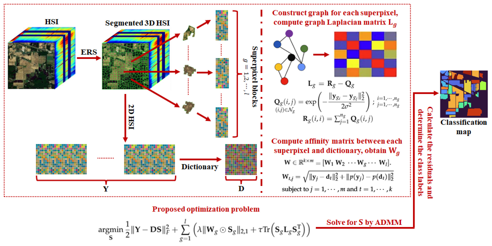
where ${\mathbf{r}}_g\in {\mathbb{R}}^c$ is a residual vector of $g^{\mathrm{th}}$ superpixel containing the class-based reconstruction errors, ${\mathbf{Y}}_g\in {\mathbb{R}}^{b\times n_g}$ denotes the pixels within that superpixel, and ${\mathbf{S}}_{g_i}$ refers to the coefficient matrix of superpixel belonging to the $i^{\mathrm{th}}$ class, respectively. Finally, the label of this superpixel is determined as the class that yields the minimum reconstruction error in ${\mathbf{r}}_g$. The pipeline of the proposed method is illustrated in Figure 1.

Algorithm 1 ADMM-based solution for the proposed SJSGR

Input: $\mathbf{Y},\mathbf{D},\mathbf{W},\gamma ,\lambda ,\tau ,\mu =0.1,ϵ=0.1$ Initialization: $\mathbf{B}={({\mathbf{D}}^{\mathrm{T}}\mathbf{D}+2\mathbf{I})}^{-1},{\mathbf{S}}^{\left(0\right)}=\mathbf{B}{\mathbf{D}}^{\mathrm{T}}\mathbf{Y},{\mathbf{V}}_1^{\left(0\right)}=\mathbf{D}\mathbf{S},{\mathbf{V}}_2^{\left(0\right)}={\mathbf{V}}_3^{\left(0\right)}=\mathbf{S},{\mathbf{P}}_1^{\left(0\right)}={\mathbf{P}}_2^{\left(0\right)}={\mathbf{P}}_3^{\left(0\right)}=0,u=0$    1: for $g=1$ to l do    2:  ${\mathbf{L}}_g={\mathbf{R}}_g-{\mathbf{Q}}_g$    3: end for    4: repeat    5:  ${\mathbf{S}}^{(u+1)}=\mathbf{B}\left[{\mathbf{D}}^{\mathrm{T}}({\mathbf{V}}_1^{\left(u\right)}+{\mathbf{P}}_1^{\left(u\right)})+({\mathbf{V}}_2^{\left(u\right)}+{\mathbf{P}}_2^{\left(u\right)})+({\mathbf{V}}_3^{\left(u\right)}+{\mathbf{P}}_3^{\left(u\right)})\right]$    6:  ${\mathbf{V}}_1^{(u+1)}={\displaystyle \frac{1}{1+\mu }}\left(\mathbf{Y}+\mu (\mathbf{D}{\mathbf{S}}^{(u+1)}-{\mathbf{P}}_1^{\left(u\right)})\right)$    7:  for $g=1$ to l do    8:   ${\mathbf{V}}_{2_g}^{(u+1)}=\mathrm{vector}\_\mathrm{soft}\_\mathrm{row}({\mathbf{S}}_g^{(u+1)}-{\mathbf{P}}_{2_g}^{\left(u\right)},\lambda /\mu ,{\mathbf{W}}_g)$    9:   ${\mathbf{V}}_{3_g}^{(u+1)}=\mu ({\mathbf{S}}_g^{(u+1)}-{\mathbf{P}}_{3_g}^{\left(u\right)}){(2\tau {\mathbf{L}}_g+\mu \mathbf{I})}^{-1}$  10:  end for  11:  ${\mathbf{P}}_1^{(u+1)}={\mathbf{P}}_1^{\left(u\right)}-\mathbf{D}{\mathbf{S}}^{(u+1)}+{\mathbf{V}}_1^{(u+1)}$  12:  ${\mathbf{P}}_2^{(u+1)}={\mathbf{P}}_2^{\left(u\right)}-{\mathbf{S}}^{(u+1)}+{\mathbf{V}}_2^{(u+1)}$  13:  ${\mathbf{P}}_3^{(u+1)}={\mathbf{P}}_3^{\left(u\right)}-{\mathbf{S}}^{(u+1)}+{\mathbf{V}}_3^{(u+1)}$  14:  $\mathrm{res}\_\mathrm{p}={\parallel \left[{\mathbf{V}}_1^{(u+1)};{\mathbf{V}}_2^{(u+1)};{\mathbf{V}}_3^{(u+1)}\right]-\left[\mathbf{D}{\mathbf{S}}^{(u+1)};{\mathbf{S}}^{(u+1)};{\mathbf{S}}^{(u+1)}\right]\parallel }_F$  15:  $\mathrm{res}\_\mathrm{d}={\parallel \left[{\mathbf{V}}_1^{(u+1)};{\mathbf{V}}_2^{(u+1)};{\mathbf{V}}_3^{(u+1)}\right]-\left[{\mathbf{V}}_1^{\left(u\right)};{\mathbf{V}}_2^{\left(u\right)};{\mathbf{V}}_3^{\left(u\right)}\right]\parallel }_F$  16:  Update iteration: $u\leftarrow u+1$  17: until $\left(\mathrm{res}\_\mathrm{p}\le ϵOR\mathrm{res}\_\mathrm{d}\le ϵ\right)$ Output: The coefficient matrix $\mathbf{S}$. Note: The function $\mathrm{vector}\_\mathrm{soft}\_\mathrm{row}(\mathbf{A},\psi ,\mathbf{Z})$ provides weighted row-wise sparsity. Let $\mathbf{a}$ and $\mathbf{z}$ be the arbitrary row-vectors of $\mathbf{A}$ and $\mathbf{Z}$, respectively. Then, the function evaluates $\mathbf{a}\mapsto {\displaystyle \frac{max\left({\parallel \mathbf{a}\parallel }_2-\psi {\parallel \mathbf{z}\parallel }_2,0\right)}{max\left({\parallel \mathbf{a}\parallel }_2-\psi {\parallel \mathbf{z}\parallel }_2,0\right)+\psi {\parallel \mathbf{z}\parallel }_2}}\mathbf{a}.$

3. Experimental Results

3.1. Datasets

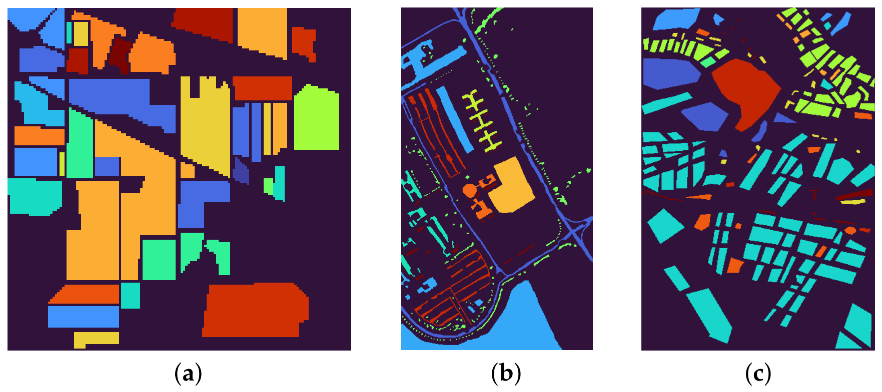
Experiments are conducted on three different hyperspectral datasets called Indian Pines (IP) [42], Pavia University (PU) [43] and Fanglu (FL) [44]. A summary of these datasets is presented in

Table 1. Comparison of the IP, PU and FL datasets.

Dataset	Sensor	Size	Spectral Res.	Spatial Res.	Num. of Classes	Num. of Samples
IP	AVIRIS	$145\times 145\times 200$	∼10 nm	20 m	16	10,366
PU	ROSIS	$610\times 340\times 103$	∼4 nm	1.3 m	9	42,776
FL	APHI	$512\times 348\times 80$	∼8 nm	2.25 m	10	53,734

. It is seen that each dataset has distinct characteristics in terms of size, resolution, available classes and number of samples. Additionally, these are acquired by the different sensors, such as the Airborne Visible/Infrared Imaging Spectrometer (AVIRIS), Reflective Optics System Imaging Spectrometer (ROSIS) and Aerosol Pushbroom Hyperspectral Imager (APHI) for the IP, PU and FL datasets, respectively. The use of datasets with different characteristics in HSIC is important because the accuracy results on these datasets demonstrate the generalization capability of the methods. More detailed information about the IP, PU and FL datasets including class names and available number of samples, are given in

Table 2. IP class distributions, with background colors correspond to the ground-truth class colors.

Class	Name	Samples
1	Alfalfa	54
2	Corn-notill	1434
3	Corn-mintill	834
4	Corn	234
5	Grass-pasture	497
6	Grass-trees	747
7	Grass-pasture-mowed	26
8	Hay-windrowed	489
9	Oats	20
10	Soybean-notill	968
11	Soybean-mintill	2468
12	Soybean-clean	614
13	Wheat	212
14	Woods	1294
15	Buildings-Grass-Trees-Drives	380
16	Stone-Steel-Towers	95

,

Table 3. PU class distributions, with background colors correspond to the ground-truth class colors.

Class	Name	Samples
1	Asphalt	6631
2	Meadows	18,649
3	Gravel	2099
4	Trees	3064
5	Painted metal sheets	1345
6	Bare soil	5029
7	Bitumen	1330
8	Self-Blocking Bricks	3682
9	Shadows	947

and

Table 4. FL class distributions, with background colors correspond to the ground-truth class colors.

Class	Name	Samples
1	Masson pine	5806
2	Bamboo forest	2318
3	Tea plant	28,428
4	Reed	214
5	Paddy	6809
6	Sweet potato	817
7	Caraway	429
8	Weed	1861
9	Water body	6141
10	Building/Road	911

, respectively. Also, corresponding ground-truth (GT) images of the IP, PU and FL datasets are presented in Figure 2.

3.2. Performance Metrics

The performance of the proposed SJSGR is compared with several methods in the literature such as JSRC [8], CCJSR [14], MSSGF [19], LCJS-WLR [21], SGR [24], SGL [26] and WSGR [25]. It should be noted that the source codes of methods JSRC, CCJSR, SGR, SGL and WSGR are publicly available, while methods MSSGF and LCJS-WLR are the authors’ own methods. The codes for the other methods mentioned in the literature review of the sparse and graph-based studies, except for [28], were not publicly available, and therefore were not used in the experimental study. As for [28], because its methodology differs in scope from the proposed method and other methods compared, it was not included in the experimental study.

The performance of all methods are evaluated and compared in terms of class-based accuracy, overall accuracy (OA), average accuracy (AA) and Cohen’s kappa coefficient ($\kappa$) metrics. Here, class accuracy represents the ratio of correctly classified samples to the total number of samples in a given class. AA denotes the sum of the class-based accuracies divided by the total number of classes. OA is the ratio of correctly classified samples to the total number of samples. The kappa coefficient is a statistical metric that assesses classification performance by normalizing the difference between OA and the accuracy expected by chance. All experiments are repeated ten times using randomly chosen training dictionaries, and then the results are averaged to minimize the bias.

3.3. Parameter Tuning of SJSGR

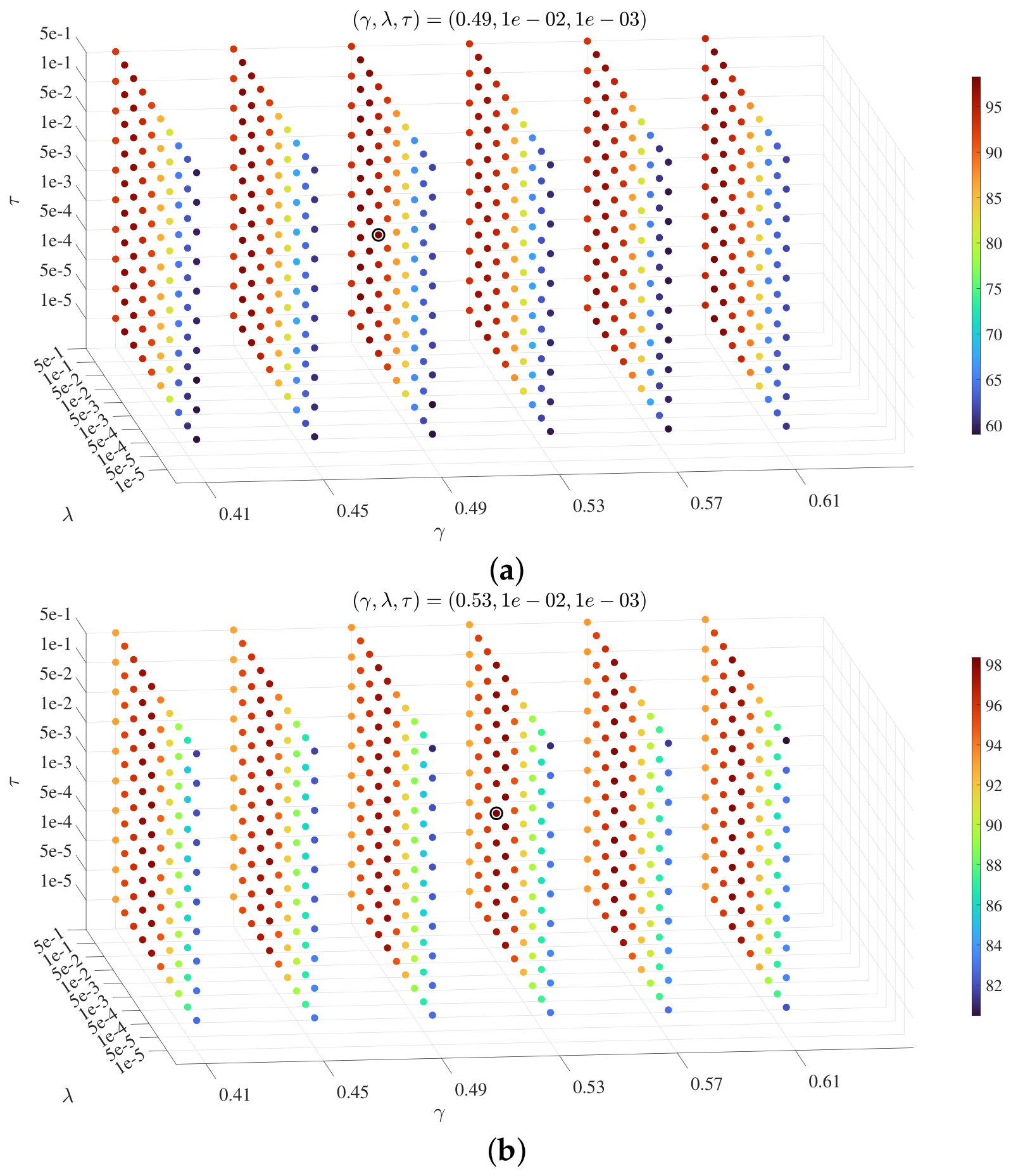
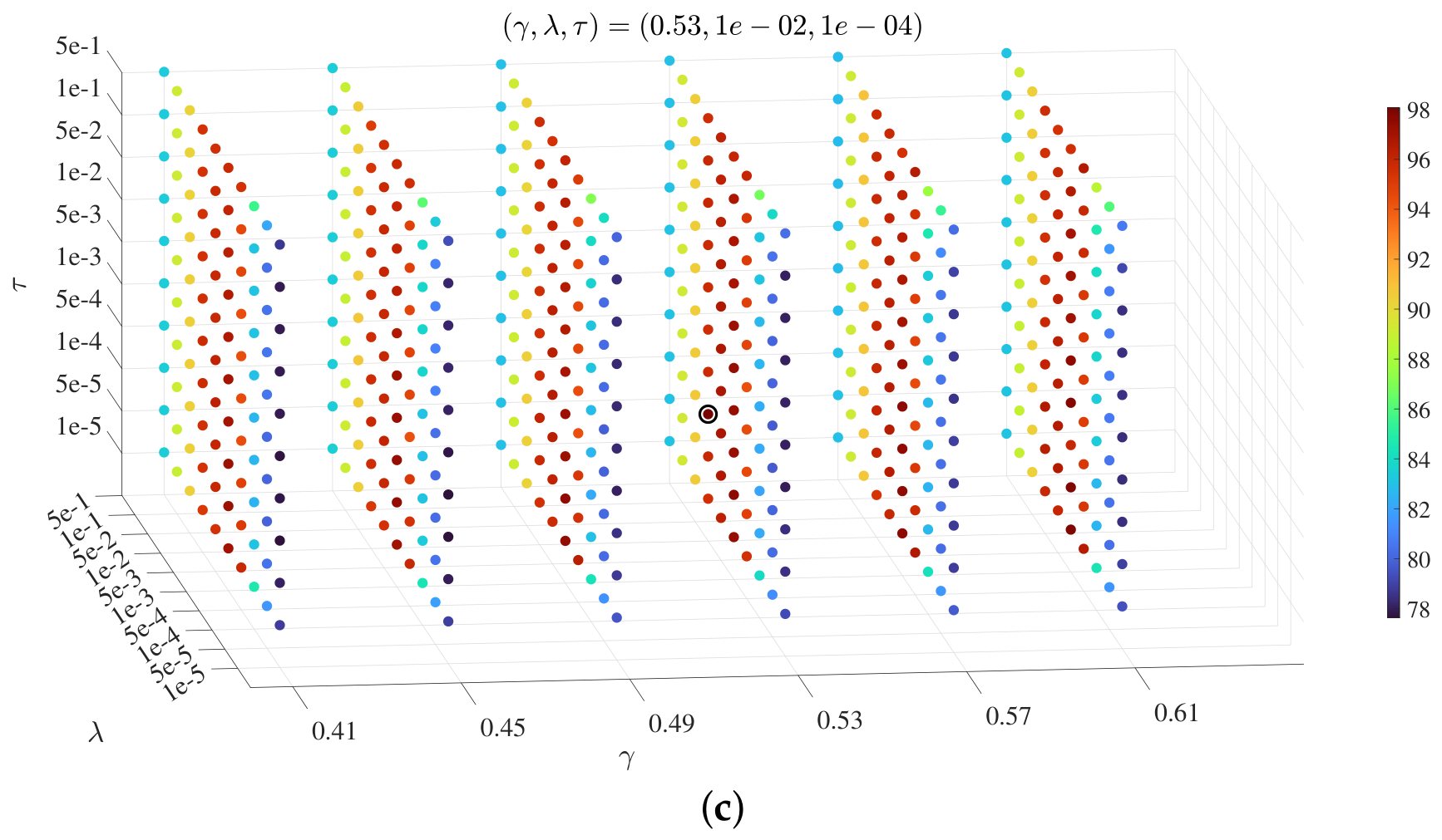
The corresponding parameters of the other methods are fine-tuned for all datasets to perform a fair comparison. As for the SJSGR, it has several important parameters: $\gamma$ for the number of superpixels, and $\lambda$ and $\tau$ for the joint-sparse and graph regularization terms, respectively. To specify the optimal parameters for each dataset, we applied a grid search over the ranges of $\gamma =\{0.41,0.45,0.49,0.53,0.57,0.61\}$ and $(\lambda ,\tau )=$ $\{{10}^{-5},5\times {10}^{-5},{10}^{-4},5\times {10}^{-4},{10}^{-3},5\times {10}^{-3},{10}^{-2},5\times {10}^{-2},{10}^{-1},5\times {10}^{-1}\}$, and then we record the OA results. Figure 3 presents the observed results in terms of scatter plots. As can be seen from the colorbars indicated in the plots, high results were attained at many points. However, the highest OA value was obtained at only one intersection point for each dataset. In accordance with these observations given in Figure 3, $\gamma$ was set to $0.49$ for the IP, and $0.53$ for the PU and FL datasets, respectively. For $\lambda$, it was adjusted to ${10}^{-2}$ for all datasets. Finally, the parameter $\tau$ was tuned as ${10}^{-3}$ for the IP and PU datasets, and ${10}^{-4}$ for the dataset FL, respectively. The optimal parameters of the datasets are given in

Table 5. Optimal parameters of SJSGR across the datasets.

Parameter	IP	PU	FL
$\gamma$	$0.49$	$0.53$	$0.53$
$\lambda$	${10}^{-2}$	${10}^{-2}$	${10}^{-2}$
$\tau$	${10}^{-3}$	${10}^{-3}$	${10}^{-4}$

. A closer examination of Figure 3 reveals that $\lambda$ has the strongest influence on the OA results among all parameters. This effect is followed by the $\gamma$ parameter. On the other hand, $\tau$ does not noticeably affect the OA results. However, it preserves their consistency. Since this parameter is responsible for graph regularization, its effect should be further analyzed through an ablation study.

3.4. Ablation Study

In order to assess the influence of the graph regularization term controlled by the $\tau$ parameter, we performed an ablation study by comparing the proposed SJSGR method with a modified version called SJS where the graph regularization term is discarded.

Table 6. Ablation study of the proposed SJSGR across the datasets. Bold and underlined values indicate the best and second-best results, respectively.

Metric	SJS			SJSGR
	IP	PU	FL	IP	PU	FL
OA	97.90	97.10	98.02	98.12	98.04	98.26
AA	98.17	91.89	93.92	98.45	96.36	94.89

presents the results obtained on the datasets in terms of OA and AA metrics. It is seen that a slight increase is obtained in the OA and AA results for the IP dataset. As for the PU dataset, the OA and AA results are improved by approximately $1\%$ and $4.5\%$, respectively. This improvement is due to the use of the graph regularization term. For the FL dataset, OA shows a slight enhancement, whereas AA improves by approximately $1\%$. Therefore, these ablation studies demonstrate that the graph regularization term improves the results slightly or moderately depending on the dataset, thus ensuring consistency.

3.5. Results

Here, both quantitative and qualitative results of the IP, PU and FL datasets are given, respectively.

3.5.1. Indian Pines

Table 7. Accuracy results of the methods across the IP dataset. Bold and underlined values indicate the best and second-best results, respectively, while background colors correspond to the ground-truth class colors.

IP (10% LABELED TRAINING SAMPLES PER CLASS)
Class	Train/Test	JSRC	CCJSR	MSSGF	LCJSWLR	SGR	WSGR	SGL	SJSGR
1	6/48	95.00	94.17	98.33	93.33	89.58	97.58	96.17	98.33
2	144/1290	95.61	94.54	97.52	92.99	95.76	95.18	94.43	96.65
3	84/750	95.09	94.64	97.25	92.85	94.83	93.21	96.32	96.48
4	24/210	92.48	94.67	96.86	96.76	93.81	100	95.52	97.76
5	50/447	92.57	94.81	96.51	93.69	95.75	95.53	98.17	98.52
6	75/672	95.12	98.39	98.66	97.65	98.78	97.59	99.43	99.32
7	3/23	69.57	60.87	96.52	83.48	93.91	100	100	100
8	49/440	99.50	99.82	100	98.41	100	100	99.77	99.77
9	2/18	8.89	40.00	64.44	38.89	10.00	100	100	100
10	97/871	91.02	94.28	92.95	90.40	92.38	94.75	94.23	95.65
11	247/2221	96.01	96.21	97.71	98.00	98.21	98.22	98.38	98.82
12	62/552	89.93	89.96	97.14	92.97	96.84	96.25	94.53	96.87
13	22/190	86.42	96.95	99.58	99.47	99.69	99.89	99.89	99.47
14	130/1164	98.61	99.18	99.78	100	99.90	99.48	99.91	100
15	38/342	93.80	93.80	96.67	98.60	98.16	100	98.88	98.72
16	10/85	75.53	92.71	97.65	97.18	99.76	99.29	93.18	98.82
OA (±std)		94.53	95.59	97.46	95.76	96.91	97.18	97.31	98.12
		$\pm 0.38$	$\pm 0.70$	$\pm 0.29$	$\pm 0.40$	$\pm 0.30$	$\pm 0.52$	$\pm 0.28$	$\pm 0.25$
AA (±std)		85.95	89.69	95.47	91.54	91.09	97.94	97.43	98.45
		$\pm 2.86$	$\pm 1.72$	$\pm 2.86$	$\pm 2.55$	$\pm 0.56$	$\pm 0.36$	$\pm 0.31$	$\pm 0.29$
$\kappa$ (±std)		93.77	94.97	97.14	95.17	96.51	96.82	96.94	97.83
		$\pm 0.43$	$\pm 0.80$	$\pm 0.33$	$\pm 0.46$	$\pm 0.34$	$\pm 0.59$	$\pm 0.32$	$\pm 0.27$

presents the achieved accuracy results of the methods under $10\%$ labeled training samples per class for the IP dataset. It is seen that JSRC provides the lowest accuracy results compared to the other methods. Incorporating the correlation coefficients between the training samples and local patches into the residual calculation, CCJSR outperforms JSRC by nearly $1\%$ and $4\%$ in terms of OA and AA. By considering local low-rank structure of each superpixel and imposing locality-preserving framework, LCJSWLR achieves a similar OA result compared to CCJSR, but obtains about $2\%$ higher AA. The performance of LCJSWLR is followed by SGR, which provides nearly $1.2\%$ higher OA, but attains a lower AA than LCJSWLR. A weighted extension of SGR, called WSGR, provides slightly higher OA and approximately $7\%$ better AA than SGR. Another graph regularization-based method called SGL has competitive accuracy results compared to WSGR. While SGL slightly outperforms WSGR in terms of OA, WSGR exceeds the AA result of SGL relatively. A similar condition is also observed among SGL and MSSGF. It is seen that MSSGF provides slightly higher OA than SGL, but SGL has nearly $2.5\%$ better AA than MSSGF. Regarding the proposed SJSGR, it exceeds the best OA result by approximately $0.7\%$ and the best AA result by about $0.5\%$ in other methods. Therefore, the proposed method achieves the highest OA and AA results for the IP dataset.

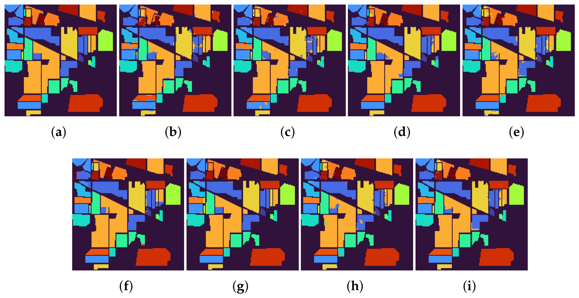
In addition to the given quantitative findings regarding the IP dataset, we also present the qualitative observations for all methods. Figure 4 demonstrates the classification maps of the methods with OAs under the same train/test splitting percentages adjusted for this dataset. It is seen that the proposed SJSGR produces a classification map which is closer to the corresponding ground-truth (GT) map of the dataset. Compared to the other methods, SJSGR provides smoother intra-class local regions and sharper inter-class transitions. These visual representations also reveal the efficacy of the proposed method.

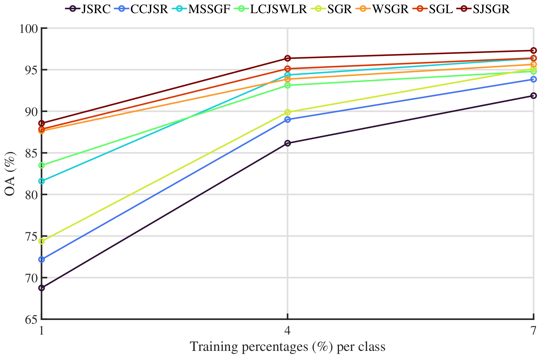
Apart from the aforementioned results, we also performed an experiment to observe the OA results of the methods under low-training-sample distributions such as $1\%$, $4\%$ and $7\%$ labeled samples per class. As seen from Figure 5, performances of the methods gradually increase depending on the training percentages. For $1\%$ sample distribution, JSRC achieves the lowest accuracy, then followed by CCJSR and SGR, respectively. It can be said that MSSGF and LCJSWLR appear to yield average-level results among all methods. While the highest OA is obtained by SJSGR, this achievement is closely followed by SGL and WSGR, respectively. For $4\%$ sample tuning, JSRC again attains the lowest OA, which is traced by CCJSR and SGR, respectively. While the other methods except SJSGR provide close results between $92.5\%$ and $95\%$, SJSGR obtains approximately $1\%$ higher OA than SGL, which provides the closest result. Finally, for $7\%$ sampling setting, it is seen that all methods attain OA results above $90\%$. Although the results of methods of this setting are close, the proposed SJSGR still appears to maintain the highest results.

3.5.2. Pavia University

Table 8. Accuracy results of the methods across the PU dataset. Bold and underlined values indicate the best and second-best results, respectively, while background colors correspond to the ground-truth class colors.

PU (1% LABELED TRAINING SAMPLES PER CLASS)
Class	Train/Test	JSRC	CCJSR	MSSGF	LCJSWLR	SGR	WSGR	SGL	SJSGR
1	67/6564	69.66	57.36	87.20	94.38	90.48	92.31	97.26	95.77
2	187/18,462	98.20	98.74	99.93	99.89	99.76	99.87	99.94	99.96
3	21/2078	83.56	80.35	90.18	99.63	84.80	93.93	78.65	99.77
4	31/3033	55.78	89.16	73.91	90.00	88.63	87.13	80.76	91.51
5	14/1331	91.10	99.53	99.68	99.68	100	100	98.39	99.25
6	51/4978	97.97	96.59	96.65	100	69.76	99.60	98.74	100
7	14/1316	89.38	61.23	99.71	98.56	97.17	100	99.24	99.64
8	37/3645	92.02	91.09	98.47	98.40	54.41	93.19	93.49	96.58
9	10/937	25.98	91.85	42.67	39.72	89.88	80.66	96.20	84.74
OA (±std)		87.37	88.53	93.82	96.82	89.07	96.47	96.25	98.04
		$\pm 0.24$	$\pm 0.76$	$\pm 0.62$	$\pm 0.39$	$\pm 1.48$	$\pm 0.45$	$\pm 0.47$	$\pm 0.20$
AA (±std)		78.18	85.10	87.60	91.14	86.10	94.08	93.63	96.36
		$\pm 1.23$	$\pm 1.84$	$\pm 0.84$	$\pm 1.51$	$\pm 1.86$	$\pm 1.32$	$\pm 0.90$	$\pm 0.97$
$\kappa$ (±std)		83.24	84.81	91.71	95.77	85.27	95.32	95.01	97.40
		$\pm 0.33$	$\pm 1.02$	$\pm 0.85$	$\pm 0.53$	$\pm 1.98$	$\pm 0.61$	$\pm 0.63$	$\pm 0.27$

demonstrates the accuracy results of the methods under $1\%$ labeled training samples per class for the PU dataset. Similar to the case of IP dataset, JSRC has the lowest OA and AA results compared to the others. The results of this method are followed by CCJSR, which provides nearly $1.2\%$ and $7\%$ higher OA and AA results, respectively. Compared to CCJSR, SGR has about $0.5\%$ and $1\%$ higher OA and AA results. Results of this method are traced by MSSGF, which obtains nearly $4.8\%$ and $1.5\%$ higher OA and AA values. It can be seen that OA of MSSGF is followed by SGL, WSGR and LCJSWLR, providing almost $2.4\%$, $2.6\%$ and $3\%$ higher results, respectively. However, as for the AA result of MSSGF, it is almost $3.5\%$, $6\%$ and $6.5\%$ outperformed by LCJSWLR, SGL and WSGR, respectively. Compared to the methods analyzed so far, it is seen that the proposed SJSGR achieves the highest OA and AA results. For example, it outperforms the best OA result by approximately $1.2\%$ and the best AA result by about $2.3\%$ in other methods.

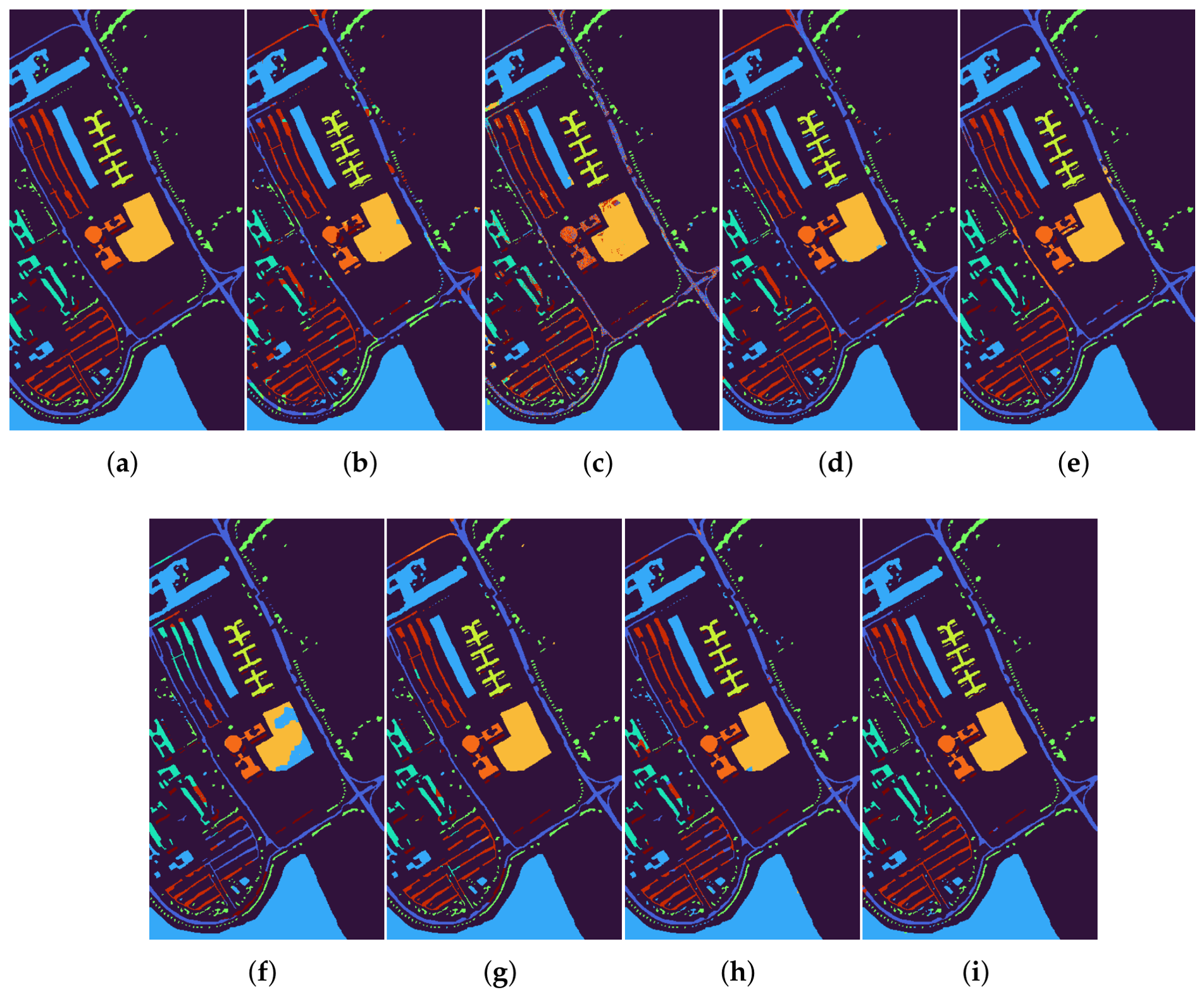
Figure 6 shows the classification maps of the methods with OAs using $1\%$ labeled training samples per class for the PU dataset. It should be noted here that this dataset has both small and large local regions as seen from the corresponding GT image. Therefore, capturing and effectively utilizing spatial information from all these regions is not an easy task for the methods. However, it is clear that the proposed SJSGR generates a classification map which is more closer to the GT map compared to the others. When the classification maps are examined, it is seen that local regions, especially those with small areas, are often inaccurately classified by other methods, whereas SJSGR classifies these regions with high accuracy, except for class 9. Hence, it can be said that the proposed method has more uniform local regions and sharper boundaries across different classes for the PU dataset, compared to the other methods.

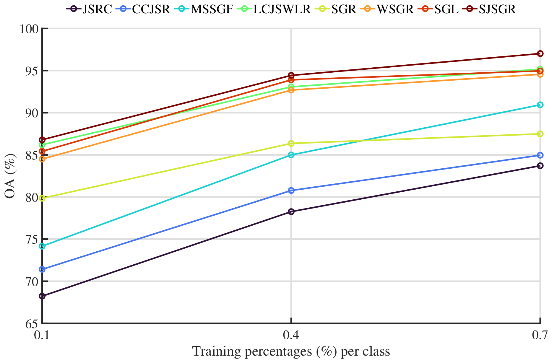
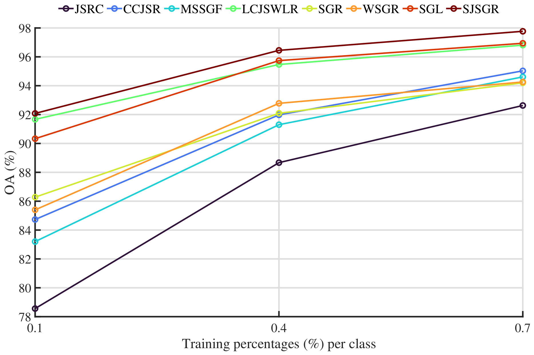
Besides both the quantitative and qualitative results above, Figure 7 shows the OA results of the methods under low-training-sample settings such as $0.1\%$, $0.4\%$ and $0.7\%$ labeled samples per class for the PU dataset. For the $0.1\%$ sampling setting, it is seen that JSRC obtains the lowest OA, which is then followed by CCJSR, MSSGF, SGR and WSGR, respectively. Starting from SGL, the OA results are observed above $85\%$, where the proposed SJSGR provides the highest OA. For the $0.4\%$ sample distribution, JSRC has again the lowest OA, which is followed by CCJSR, MSSGF and SGR, respectively. The results of WSGR, LCJSWLR, SGL and SJSGR are close to each other; however, the OA of SJSGR is closer to $95\%$ compared to the others. When the amount of labeled training samples is set to $0.7\%$, it is seen that the OA results of the methods gradually increase. While the OAs of JSRC, CCJSR and SGR remain below $90\%$, the result of MSSGF is slightly above that. At OAs of around $95\%$, WSGR, SGL and LCJSWLR obtain quite similar results. As for the proposed SJSGR, it attains an OA of approximately $97.5\%$, which is the highest result among all observations.

3.5.3. Fanglu

Table 9. Accuracy results of the methods across the FL dataset. Bold and underlined values indicate the best and second-best results, respectively, while background colors correspond to the ground-truth class colors.

FL (1% LABELED TRAINING SAMPLES PER CLASS)
Class	Train/Test	JSRC	CCJSR	MSSGF	LCJSWLR	SGR	WSGR	SGL	SJSGR
1	59/5747	96.03	96.63	96.21	99.27	99.99	100	97.85	99.39
2	24/2294	90.35	90.61	83.12	95.19	59.78	94.87	96.15	96.20
3	285/28,143	99.44	99.46	99.98	99.16	97.76	94.57	99.12	99.53
4	3/211	91.75	88.72	100	91.28	2.09	100	100	98.67
5	69/6740	89.97	95.51	97.15	99.57	100	99.99	99.99	99.75
6	9/808	62.77	75.52	75.17	78.76	87.28	95.32	72.33	81.67
7	5/424	56.18	73.02	78.58	99.42	99.91	100	91.20	100
8	19/1842	72.73	77.99	66.54	70.62	52.33	87.34	82.46	81.10
9	62/6079	97.62	99.18	98.65	98.15	99.05	99.05	98.75	98.65
10	10/901	48.39	90.28	90.34	92.08	100	96.56	78.65	93.96
OA (±std)		94.55	96.73	96.37	97.43	94.54	96.23	97.45	98.26
		$\pm 0.31$	$\pm 0.30$	$\pm 0.44$	$\pm 0.52$	$\pm 0.75$	$\pm 0.87$	$\pm 0.65$	$\pm 0.37$
AA (±std)		80.52	88.69	88.58	92.35	79.82	96.77	91.65	94.89
		$\pm 1.79$	$\pm 1.78$	$\pm 1.38$	$\pm 1.38$	$\pm 1.49$	$\pm 0.90$	$\pm 0.93$	$\pm 1.29$
$\kappa$ (±std)		91.77	95.09	94.54	96.33	92.02	94.53	96.42	97.38
		$\pm 0.49$	$\pm 0.46$	$\pm 0.69$	$\pm 0.78$	$\pm 1.09$	$\pm 1.23$	$\pm 0.96$	$\pm 0.56$

shows the accuracy results of the methods over the FL dataset using $1\%$ labeled training samples per class. It can be seen that JSRC and SGR provide quite similar OA results, but JSRC attains nearly $0.7\%$ higher AA than SGR. In terms of OA, WSGR follows the results of these two methods. As for MSSGF, it obtains a quite similar OA compared to WSGR. Following MSSGF, CCJSR provides approximately $0.4\%$ higher OA, and then this improvement is followed by LCJSWLR and SGL, respectively. Additionaly, it can be said that LCJSWLR and SGL achieve almost identical OA results. As for the AA results of the methods, MSSGF and CCJSR outperform JSRC by about $8\%$. Following these methods, approximately $3\%$ improvement is achieved by SGL. As for the AA of LCJSWLR, it is nearly $0.7\%$ higher than the one of SGL. As seen from the AA of the proposed SJSGR, it outperforms the AA of LCJSWLR by about $2.5\%$. Finally, WSGR obtains the highest AA result for the FL dataset. It provides approximately $2\%$ higher AA than the proposed SJSGR. Unlike the other two datasets, IP and PU, it can be seen that there is not much consistency between the OA and AA results of the methods in this dataset. The relatively inconsistent performance observed on this dataset may be attributed to its class imbalance, fewer spectral features and spectral similarity between classes, which are the challenging cases for the classifiers. However, when the results of the proposed SJSGR method are analyzed, it is clear that it provides the highest OA and the second highest AA results.

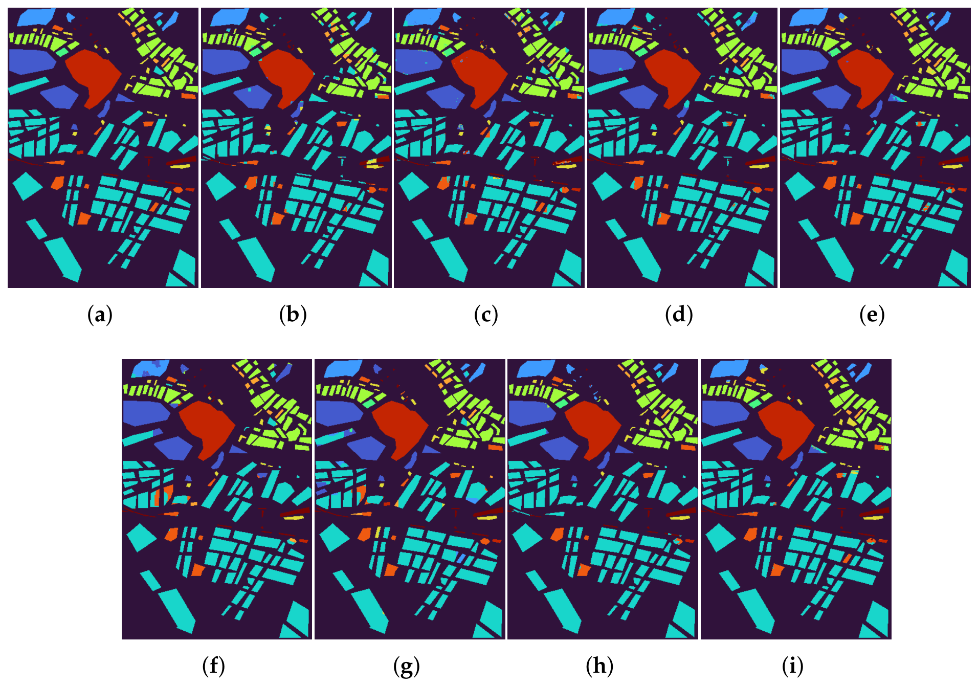
The visual representations of the methods under $1\%$ labeled training samples per class are given in Figure 8 for the FL dataset. Similar to the case of PU, this dataset has also both small and large local areas as seen from the corresponding GT image. As seen from the OA results, the proposed SJSGR obtains a classification map which is more similar to the GT map compared to remaining ones. Examining the results in Table 9, it is clear that the reason for the higher AA result of WSGR compared to SJSGR is due to its effective classification performance in class 6. This effect is also clearly visible when analyzing the maps of methods WSGR and SJSGR, where relatively small regions of this class are more correctly classified by WSGR. However, it can be said that SJSGR provides more homogeneous spatial regions except for this class.

Figure 9 gives the performance comparison of the methods in terms of OA by varying the percentages of labeled training samples per class such as $0.1\%$, $0.4\%$ and $0.7\%$ for the FL dataset. As seen for the $0.1\%$ sampling percentage, JSRC yields the lowest OA among all methods. Following this, MSSGF, CCJSR, WSGR and SGR appear to provide average-level OA results, respectively. It can be seen that the OAs of these methods are approximately between $83.5\%$ and $86\%$. As for the remaining ones, called SGL, LCJSWLR and SJSGR, the results are observed as above $90\%$, where SJSGR achieves the highest one at nearly $92\%$. For the $0.4\%$ labeled samples, it is clear that the classification performances of all methods gradually enhance. While JSRC again obtains the lowest OA, the moderate ones called MSSGF, CCJSR, SGR and WSGR yield to provide the average-level OA results, respectively. Following these, LCJSWLR and SGL have quite close OA results at around below $96\%$. Then, SJSGR obtains the highest OA which is slightly higher than $96\%$. For the last percentage rate, $0.7\%$, all methods provide high OA results, and also the results become closer to each other. While JSRC has the lowest OA over again, SGR, WSGR, MSSGF and CCJSR follow these results, respectively. As for the others, LCJSWLR and SGL have quite similar OA results around $97\%$, while SJSGR attains the highest OA close to $98\%$.

3.5.4. Computational Complexity and Time Analysis

The proposed SJSGR method has several steps to complete the whole classification process.

Table 10. Computation time of each module of the SJSGR method for the IP dataset using 10 labeled samples per class.

Module	Processing Time (s)	Percentage (%)
Superpixel construction	0.06	0.43
Weighting matrix	0.84	6.02
Graph construction	0.34	2.44
ADMM initializations	0.01	0.07
ADMM iterations	12.58	90.11
Labeling	0.13	0.93
Total	13.96	100

,

Table 11. Computation time of each module of the SJSGR method for the PU dataset using 10 labeled samples per class.

Module	Processing Time (s)	Percentage (%)
Superpixel construction	0.97	0.83
Weighting matrix	4.49	3.85
Graph construction	3.13	2.68
ADMM initializations	0.05	0.04
ADMM iterations	107.61	92.23
Labeling	0.43	0.37
Total	116.68	100

and

Table 12. Computation time of each module of the SJSGR method for the FL dataset using 10 labeled samples per class.

Module	Processing Time (s)	Percentage (%)
Superpixel construction	0.75	0.85
Weighting matrix	3.93	4.44
Graph construction	2.85	3.22
ADMM initializations	0.04	0.05
ADMM iterations	80.55	91.03
Labeling	0.37	0.41
Total	88.49	100

present the steps, and also give the approximate computation times of each one for the IP, PU and FL datasets, respectively, using 10 samples per class. It is seen that a significant portion of the running time is caused by the ADMM iterations. This iteration process includes the steps between 5 and 15 given in Algorithm 1. The complexities of steps 5 and 6 are calculated as $\mathcal{O}\left(km\right(b+k\left)\right)$ and $\mathcal{O}\left(kmb\right)$, respectively. As for steps 8 and 9, which need to be computed for each superpixel, the corresponding time complexities are given as $\mathcal{O}\left(k{n}_g\right)$ and $\mathcal{O}\left(k{n}_g^2\right)$, respectively. It should be noted that the term ${(2\tau {\mathbf{L}}_g+\mu \mathbf{I})}^{-1}$ in step 9 is computed once during the graph construction stage, and then fixed over the course of the iterations. Due to the presence of l superpixels in total, these can be rewritten as $\mathcal{O}\left(k{\sum }_{g=1}^l{n}_g\right)$ and $\mathcal{O}\left(k{\sum }_{g=1}^l{n}_g^2\right)$, accordingly. Step 11 has a complexity of $\mathcal{O}\left(kmb\right)$, and steps 12 and 13 have $\mathcal{O}\left(km\right)$. Finally, the computational complexities of steps 14 and 15 require $\mathcal{O}\left(kmb\right)$ and $\mathcal{O}(bm+km)$, respectively. Therefore, the proposed SJSGR method has an overall complexity of $\mathcal{O}\left(km(b+k)\right)+\mathcal{O}\left(kmb\right)+\mathcal{O}\left(k{\sum }_{g=1}^l{n}_g\right)+\mathcal{O}\left(k{\sum }_{g=1}^l{n}_g^2\right)+\mathcal{O}\left(kmb\right)+\mathcal{O}\left(km\right)+\mathcal{O}\left(kmb\right)+\mathcal{O}(bm+km)$ for the per ADMM iteration, consuming the most of the total running time. Since ${\sum }_{g=1}^l{n}_g$ is equal to the total pixel count m, the term $\mathcal{O}\left(k{\sum }_{g=1}^l{n}_g\right)$ is reduced to $\mathcal{O}\left(km\right)$. By retaining only the dominant ones, the complexity of SJSGR per ADMM iteration can be given as $\mathcal{O}\left(km(b+k)+k{\sum }_{g=1}^l{n}_g^2\right)$.

The computational efficiency of the proposed and competing methods was evaluated by comparing their execution times. All experiments were conducted on the same hardware platform consisting of an Intel Core i7-12700K processor (3.60 GHz) and 128 GB of RAM to ensure a fair comparison. The execution times obtained with ten labeled samples per class are presented in

Table 13. Comparison of computational time (in seconds) of the methods using ten labeled samples per class across the datasets.

Dataset	JSRC	CCJSR	MSSGF	LCJSWLR	SGR	WSGR	SGL	SJSGR
IP	2.19	15.85	3.98	59.12	3.37	9.12	14.34	13.96
PU	25.14	58.48	39.46	522.95	17.58	26.51	122.39	116.68
FL	30.6	74.18	37.77	434.26	16.56	23.09	91.26	88.49

for all datasets. It is clearly observed that the LCJSWLR method requires the highest computational time across all datasets. This is mainly due to its complex optimization procedure and, more importantly, the low-rank minimization performed within each superpixel, which significantly increases the computational cost. The JSRC method achieves the lowest computational time on the IP dataset, whereas the SGR method is faster on the other datasets. When the computational times of the methods that achieve classification accuracies closest to the proposed SJSGR method, namely SGL, WSGR, LCJSWLR, and MSSGF, are examined, the LCJSWLR is the slowest among them, as mentioned before. Compared with the SGL method, the SJSGR exhibits slightly lower computational times for all datasets. Regarding the remaining methods, WSGR and MSSGF are both several times faster than the SJSGR method across the datasets.

3.5.5. Comparison with the Deep Learning-Based Models

Although the proposed SJSGR method is based on a traditional machine learning classifer, its performance was also compared with the several deep learning-based methods such as SpectralFormer (https://github.com/danfenghong/IEEE_TGRS_SpectralFormer, accessed on 27 July 2026) [45], 3DSS−Mamba (https://github.com/IIP-Team/3DSS-Mamba, accessed on 27 July 2026) [46], HybridSN (https://github.com/gokriznastic/HybridSN, accessed on 28 July 2026) [47], SSEFN (https://github.com/liushuang963/SSEFN, accessed on 29 July 2026) [48] and DSFormer (https://github.com/YichuXu/DSFormer, accessed on 29 July 2026) [49]. In order to perform fair comparisons, the same training and test indices, utilized in the previous experiments, were adopted for each dataset. Specifically, $10\%$ and $1\%$ of the samples from each class were employed for training in the IP and PU datasets, respectively, while the remaining samples used for testing. It should be noted that the FL dataset was not used for the comparison since the chosen DL-based models have no optimization parameters for this data. As for the IP and PU datasets, the training parameters of these models were tuned as the values provided in the related original articles. The results were recorded in terms of OA, AA and $\kappa$, respectively.

Table 14. Classification performance (%) of different methods on two hyperspectral datasets. Bold and underlined values indicate the best and second-best results, respectively.

Method	IP			PU
	OA	AA	$\mathit{\kappa }$	OA	AA	$\mathit{\kappa }$
SpectralFormer	90.90	83.85	89.61	86.03	80.88	81.18
3DSS−Mamba	94.43	91.98	93.64	90.94	85.66	87.92
HybridSN	98.12	95.97	97.83	94.34	90.97	92.53
SSEFN	97.64	97.91	97.31	97.47	96.78	96.64
SJSGR	98.14	98.45	97.88	98.04	96.36	97.40
DSFormer	98.27	96.69	98.02	98.55	97.52	98.08

presents the results for both of the datasets. It is seen that the DSFormer achieves the highest OA and $\kappa$ results, which are being closely followed by the SJSGR method for the IP dataset. As for the AA value, the SJSGR provides the best result, which is traced by the SSEFN model. Similarly, the DSFormer attains the highest metrics, which are followed by the SJSGR and SSEFN methods, respectively, for the PU dataset.

4. Discussion

The results obtained from the exhaustive experiments are discussed here. It should be noted that it is not possible to generalize the results of methods other than JSRC and the proposed SJSGR framework, because the performances of the methods vary depending on the datasets.

Throughout the experiments, it was observed that JSRC yields to provide lowest accuracy results. This method considers the spatial information of a HSI using a fixed-size patch constructed around a given test sample without assigning distinct weight to each neighbor. Such an assumption may cause misclassification of this test sample if it is around class borders. In such a case, the impact of pixels belonging to different classes may become more dominant. Apart from this, JSRC only applies a sparsity constraint which takes into account the spectral similarity of pixels, but ignores the local manifold structure of that patch. By incorporating the correlation coefficients between the training samples and local patches into the residual calculation, the CCJSR method outperforms JSRC across all datasets. This observation reveals the idea that such correlation may improve the results by inserting it into the optimization problem. As observed, MSSGF considerably outperforms CCJSR for the IP and FL datasets, but their corresponding results are quite competitive for the FL dataset. Since MSSGF utilizes multiscale superpixels, the spatial information is effectively employed in two ways. The first one is to obtain more homogeneous local regions through superpixels, and the second one is to capture local information in a broad range through multiscale superpixels. The use of these extensive spatial information with sparsity constraint enhances the results. The results indicate that LCJSWLR is superior to the MSSGF, except for the IP dataset. This method simultaneously employs weighted joint-sparse and low-rank regularizations in homogeneous regions obtained by single-scale superpixel segmentation. A unified utilization of such regularization terms enables the coefficient matrix to be more informative than the use of sparsity constraint only. Therefore, the results are improved compared to the MSSGF for the PU and FL datasets. The reason for obtaining lower accuracy results for the IP dataset may be the ineffective use of spatial information.

Besides these sparsity-constraint-based methods, SGR is generally superior to JSRC and CCJSR, but is usually outperformed by LCJSWLR and MSSGF depending on the dataset. SGR computes the coefficient matrix of all pixels by introducing sparse-regularization only. In this stage, it does not consider the neighborhood information of these pixels. After that, it constructs a graph Laplacian matrix based on the coefficient matrix. By utilizing both coefficient and graph Laplacian matrices, a prediction function is evaluated. Due to ignoring neighborhood information and local manifold structure of the data, SGR yields limited performance. As an extension of SGR, the method WSGR provides higher accuracy results than SGR. Also, the results of WSGR become competitive with the ones of MSSGF and LCJSWLR. The reason for this observation could be the incorporation of spatial information in WSGR since it applies a weighting scheme to the central pixel and its neighborhoods in a fixed-size patch. In this way, each pixel of a HSI is transformed into the weighted one, and then the weighted pixels are processed using the same procedure as in SGR. As for the last graph regularization-based method, SGL, it provides competitive performance compared to the WSGR, MSSGF and LCJSWLR, which are the methods providing high accuracy results across the datasets. The satisfying results of SGL can be given as follows. It extracts additional descriptive features from each superpixel, and then these features are used to construct graphs between two linked superpixels. In this way, both local spatial information and global structure of the data are considered for the purpose of classification.

Based on the analyses conducted so far, the performances of methods vary depending on the dataset. For the proposed SJSGR, it was observed that the highest OA results are observed for all different training sample distributions across the datasets. Except for the FL dataset, the highest AA results are also obtained by SJSGR. The reasons behind this performance can be given as follows: It utilizes superpixels to capture the spatial information in a HSI, effectively. The proposed optimization problem incorporates the correlation between each superpixel-block and training dictionary. In this way, the potential of selecting more appropriate training samples is promoted. Due to the joint-sparse regularization term, the pixels within each superpixel are represented by the same training samples. Finally, the graph Laplacian-based regularization term enforces the coefficient matrix to have similar codes among the pixels of the superpixel. To sum up, unifying all these constraints in an optimization framework enhances the discriminative structure of the coefficient matrix.

Regarding the proposed SJSGR method, long execution times are observed, particularly on the PU and FL datasets. This is primarily attributed to the large number of generated superpixels resulting from the larger image sizes. Since the SJSGR method performs joint-sparse and graph regularization-based optimization within each superpixel, the computational cost increases as the number of superpixels grows. Although the WSGR and MSSGF methods require less computation time, their classification performance across all datasets remains inferior to that of the proposed method. This performance gap becomes even more pronounced under limited-training-sample conditions. The SGL method also achieves lower classification accuracies than the proposed method while requiring slightly more computation time. Overall, the experimental results demonstrate that although the proposed method requires longer execution times for datasets with large spatial dimensions, this additional computational cost is largely compensated by its higher classification accuracy results compared with the other methods.

Finally, the comparison with recent deep learning models shows that the SJSGR method provides competitive classification performance across the datasets. While several models attain slightly higher accuracies on certain datasets, the proposed method consistently achieves comparable or higher results without depending on the deep feature learning. These observations demonstrate that the proposed framework maintains an effective alternative, especially when the labeled training samples are limited.

5. Conclusions

We propose a novel spectral–spatial HSIC method called SJSGR that efficiently captures both the local and geometric structure of each superpixel. Since neighboring pixels share similar spectral patterns, the representative coefficient matrix of these samples is expected to exhibit a joint-sparse structure. Considering this fact, we employ a weighted joint-sparse regularization to promote the selection of the most representative training samples by measuring the similarity between the samples within each superpixel and the dictionary. Besides being represented by common training samples, their representation coefficients are also expected to be similar due to high correlation among samples within each superpixel. To incorporate this information, we use a graph Laplacian regularization term which forces the neighboring samples to have similar coefficients. Experiments on three HSI datasets have shown that the SJSGR method is effective and comparable to state-of-the-art methods in the literature.

Although the proposed method demonstrates competitive classification performance, it has several limitations that should be acknowledged. First, the presence of noisy pixels in the HSI can prevent the formation of homogeneous superpixel regions. This will significantly affect the success of the method. Second, performing only single-scale segmentation may lead to a limited use of spatial information in the HSI, because the sizes of homogeneous regions within the image may vary. Finally, due to the ADMM-based optimization performed within each superpixel, increasing the number of superpixels negatively impacts the computational time of the method.

Future work may focus on using a superpixel segmentation algorithm with more precise local region modeling, which is expected to further improve the results. Additionally, a multiscale superpixel segmentation approach may be utilized to capture the spatial information more. Also, the computation time can be reduced by using faster optimization techniques.

References

1. Shaw, G.; Manolakis, D. Signal processing for hyperspectral image exploitation. IEEE Signal Process. Mag. 2002, 19, 12–16. [Google Scholar] [CrossRef]
2. Bioucas-Dias, J.M.; Plaza, A.; Camps-Valls, G.; Scheunders, P.; Nasrabadi, N.; Chanussot, J. Hyperspectral Remote Sensing Data Analysis and Future Challenges. IEEE Geosci. Remote Sens. Mag. 2013, 1, 6–36. [Google Scholar] [CrossRef]
3. Ghamisi, P.; Yokoya, N.; Li, J.; Liao, W.; Liu, S.; Plaza, J.; Rasti, B.; Plaza, A. Advances in Hyperspectral Image and Signal Processing: A Comprehensive Overview of the State of the Art. IEEE Geosci. Remote Sens. Mag. 2017, 5, 37–78. [Google Scholar] [CrossRef]
4. Manolakis, D.; Shaw, G. Detection algorithms for hyperspectral imaging applications. IEEE Signal Process. Mag. 2002, 19, 29–43. [Google Scholar] [CrossRef]
5. Melgani, F.; Bruzzone, L. Classification of hyperspectral remote sensing images with support vector machines. IEEE Trans. Geosci. Remote Sens. 2004, 42, 1778–1790. [Google Scholar] [CrossRef]
6. Benediktsson, J.; Palmason, J.; Sveinsson, J. Classification of hyperspectral data from urban areas based on extended morphological profiles. IEEE Trans. Geosci. Remote Sens. 2005, 43, 480–491. [Google Scholar] [CrossRef]
7. Chen, Y.; Jiang, H.; Li, C.; Jia, X.; Ghamisi, P. Deep Feature Extraction and Classification of Hyperspectral Images Based on Convolutional Neural Networks. IEEE Trans. Geosci. Remote Sens. 2016, 54, 6232–6251. [Google Scholar] [CrossRef]
8. Chen, Y.; Nasrabadi, N.M.; Tran, T.D. Hyperspectral Image Classification Using Dictionary-Based Sparse Representation. IEEE Trans. Geosci. Remote Sens. 2011, 49, 3973–3985. [Google Scholar] [CrossRef]
9. Fauvel, M.; Tarabalka, Y.; Benediktsson, J.A.; Chanussot, J.; Tilton, J.C. Advances in Spectral-Spatial Classification of Hyperspectral Images. Proc. IEEE 2013, 101, 652–675. [Google Scholar] [CrossRef]
10. Yu, H.; Gao, L.; Liao, W.; Zhang, B.; Zhuang, L.; Song, M.; Chanussot, J. Global Spatial and Local Spectral Similarity-Based Manifold Learning Group Sparse Representation for Hyperspectral Imagery Classification. IEEE Trans. Geosci. Remote Sens. 2020, 58, 3043–3056. [Google Scholar] [CrossRef]
11. Tu, B.; Zhou, C.; Liao, X.; Zhang, G.; Peng, Y. Spectral–Spatial Hyperspectral Classification via Structural-Kernel Collaborative Representation. IEEE Geosci. Remote Sens. Lett. 2021, 18, 861–865. [Google Scholar] [CrossRef]
12. Dundar, T.; Ince, T. Guided Filter of Random Patches Network and Relaxed-Collaborative-Representation-Based Hyperspectral Image Classification. IEEE J. Sel. Top. Appl. Earth Obs. Remote Sens. 2024, 17, 6544–6560. [Google Scholar] [CrossRef]
13. Zhang, H.; Li, J.; Huang, Y.; Zhang, L. A Nonlocal Weighted Joint Sparse Representation Classification Method for Hyperspectral Imagery. IEEE J. Sel. Top. Appl. Earth Obs. Remote Sens. 2014, 7, 2056–2065. [Google Scholar] [CrossRef]
14. Tu, B.; Zhang, X.; Kang, X.; Zhang, G.; Wang, J.; Wu, J. Hyperspectral Image Classification via Fusing Correlation Coefficient and Joint Sparse Representation. IEEE Geosci. Remote Sens. Lett. 2018, 15, 340–344. [Google Scholar] [CrossRef]
15. Gao, Q.; Lim, S.; Jia, X. Improved Joint Sparse Models for Hyperspectral Image Classification Based on a Novel Neighbour Selection Strategy. Remote Sens. 2018, 10, 905. [Google Scholar] [CrossRef]
16. Chen, X.; Chen, N.; Peng, J.; Sun, W. Local Matrix Feature-Based Kernel Joint Sparse Representation for Hyperspectral Image Classification. Remote Sens. 2022, 14, 4363. [Google Scholar] [CrossRef]
17. Chen, Y.; Nasrabadi, N.M.; Tran, T.D. Hyperspectral Image Classification via Kernel Sparse Representation. IEEE Trans. Geosci. Remote Sens. 2013, 51, 217–231. [Google Scholar] [CrossRef]
18. Fang, L.; Li, S.; Kang, X.; Benediktsson, J.A. Spectral–Spatial Classification of Hyperspectral Images with a Superpixel-Based Discriminative Sparse Model. IEEE Trans. Geosci. Remote Sens. 2015, 53, 4186–4201. [Google Scholar] [CrossRef]
19. Dundar, T.; Ince, T. Sparse Representation-Based Hyperspectral Image Classification Using Multiscale Superpixels and Guided Filter. IEEE Geosci. Remote Sens. Lett. 2019, 16, 246–250. [Google Scholar] [CrossRef]
20. Zhang, A.; Pan, Z.; Fu, H.; Sun, G.; Rong, J.; Ren, J.; Jia, X.; Yao, Y. Superpixel Nonlocal Weighting Joint Sparse Representation for Hyperspectral Image Classification. Remote Sens. 2022, 14, 2125. [Google Scholar] [CrossRef]
21. Dundar, T.; Ince, T. Locality Constraint Joint-Sparse and Weighted Low-Rank Based Hyperspectral Image Classification. In 2023 10th International Conference on Recent Advances in Air and Space Technologies (RAST); IEEE: New York, NY, USA, 2023; pp. 1–6. [Google Scholar]
22. Ince, T. Superpixel-Based Graph Laplacian Regularization for Sparse Hyperspectral Unmixing. IEEE Geosci. Remote Sens. Lett. 2022, 19, 5501305. [Google Scholar] [CrossRef]
23. Liu, C.; Zhou, J.; Liang, J.; Qian, Y.; Li, H.; Gao, Y. Exploring Structural Consistency in Graph Regularized Joint Spectral-Spatial Sparse Coding for Hyperspectral Image Classification. IEEE J. Sel. Top. Appl. Earth Obs. Remote Sens. 2017, 10, 1151–1164. [Google Scholar] [CrossRef]
24. Xue, Z.; Du, P.; Li, J.; Su, H. Sparse graph regularization for robust crop mapping using hyperspectral remotely sensed imagery with very few in situ data. ISPRS J. Photogramm. Remote Sens. 2017, 124, 1–15. [Google Scholar] [CrossRef]
25. Xue, Z.; Yang, S.; Zhang, L. Weighted Sparse Graph Regularization for Spectral–Spatial Classification of Hyperspectral Images. IEEE Geosci. Remote Sens. Lett. 2021, 18, 1630–1634. [Google Scholar] [CrossRef]
26. Sellars, P.; Aviles-Rivero, A.I.; Schönlieb, C.B. Superpixel Contracted Graph-Based Learning for Hyperspectral Image Classification. IEEE Trans. Geosci. Remote Sens. 2020, 58, 4180–4193. [Google Scholar] [CrossRef]
27. Zhao, Y.; Yan, F. Hyperspectral Image Classification Based on Sparse Superpixel Graph. Remote Sens. 2021, 13, 3592. [Google Scholar] [CrossRef]
28. Yang, S.; Zhang, Y.; Jia, Y.; Zhang, W. Local Low-Rank Approximation with Superpixel-Guided Locality Preserving Graph for Hyperspectral Image Classification. IEEE J. Sel. Top. Appl. Earth Obs. Remote Sens. 2022, 15, 7741–7754. [Google Scholar] [CrossRef]
29. Wang, D.; Hu, M.; Jin, Y.; Miao, Y.; Yang, J.; Xu, Y.; Qin, X.; Ma, J.; Sun, L.; Li, C.; et al. HyperSIGMA: Hyperspectral Intelligence Comprehension Foundation Model. IEEE Trans. Pattern Anal. Mach. Intell. 2025, 47, 6427–6444. [Google Scholar] [CrossRef] [PubMed]
30. Kong, W.; Liu, B.; Bi, X.; Yu, C.; Li, X.; Chen, Y. HyperSL: A Spectral Foundation Model for Hyperspectral Image Interpretation. IEEE Trans. Geosci. Remote Sens. 2025, 63, 5513119. [Google Scholar] [CrossRef]
31. Braham, N.A.A.; Albrecht, C.M.; Mairal, J.; Chanussot, J.; Wang, Y.; Zhu, X.X. SpectralEarth: Training Hyperspectral Foundation Models at Scale. IEEE J. Sel. Top. Appl. Earth Obs. Remote Sens. 2025, 18, 16780–16797. [Google Scholar] [CrossRef]
32. Zhao, X.; Xiong, Z.; Zhu, X.X. HySens: Sensor-Agnostic Foundation Models for Hyperspectral Data. IEEE Trans. Geosci. Remote Sens. 2026, 64, 5513915. [Google Scholar] [CrossRef]
33. Lu, S.; Guo, J.; Zimmer-Dauphinee, J.R.; Nieusma, J.M.; Wang, X.; VanValkenburgh, P.; Wernke, S.A.; Huo, Y. Vision Foundation Models in Remote Sensing: A survey. IEEE Geosci. Remote Sens. Mag. 2025, 13, 190–215. [Google Scholar] [CrossRef]
34. Vaddi, R.; Phaneendra Kumar Lakshmi Narasimha, B.; Mitra, S.; Mitra, S.; Bruzzone, L.; Roy, S.K. From Traditional to Foundation Models: A Survey for Land Use and Land Cover Hyperspectral Image Classification. Wiley Interdiscip. Rev. Data Min. Knowl. Discov. 2025, 15, e70049. [Google Scholar] [CrossRef]
35. Boyd, S.; Parikh, N.; Chu, E.; Peleato, B.; Eckstein, J. Distributed Optimization and Statistical Learning via the Alternating Direction Method of Multipliers. Found. Trends Mach. Learn. 2011, 3, 1–122. [Google Scholar] [CrossRef]
36. Liu, M.; Tuzel, O.; Ramalingam, S.; Chellappa, R. Entropy rate superpixel segmentation. In CVPR 2011; IEEE: New York, NY, USA, 2011; pp. 2097–2104. [Google Scholar] [CrossRef]
37. Tu, B.; Kuang, W.; Zhao, G.; Fei, H. Hyperspectral Image Classification via Superpixel Spectral Metrics Representation. IEEE Signal Process. Lett. 2018, 25, 1520–1524. [Google Scholar] [CrossRef]
38. Xie, F.; Gao, Q.; Jin, C.; Zhao, F. Hyperspectral Image Classification Based on Superpixel Pooling Convolutional Neural Network with Transfer Learning. Remote Sens. 2021, 13, 930. [Google Scholar] [CrossRef]
39. Wang, N.; Zeng, X.; Duan, Y.; Deng, B.; Mo, Y.; Xie, Z.; Duan, P. Multi-Scale Superpixel-Guided Structural Profiles for Hyperspectral Image Classification. Sensors 2022, 22, 8502. [Google Scholar] [CrossRef] [PubMed]
40. Liao, N.; Gong, J.; Li, W.; Li, C.; Zhang, C.; Guo, B. SMALE: Hyperspectral Image Classification via Superpixels and Manifold Learning. Remote Sens. 2024, 16, 3442. [Google Scholar] [CrossRef]
41. Zhang, Y.; Duan, P.; Liang, L.; Kang, X.; Li, J.; Plaza, A. PFS3F: Probabilistic Fusion of Superpixel-Wise and Semantic-Aware Structural Features for Hyperspectral Image Classification. IEEE Trans. Circuits Syst. Video Technol. 2025, 35, 8723–8737. [Google Scholar] [CrossRef]
42. Baumgardner, M.F.; Biehl, L.L.; Landgrebe, D.A. 220 Band AVIRIS Hyperspectral Image Data Set: June 12, 1992 Indian Pine Test Site 3; Purdue University: West Lafayette, IN, USA, 2015. [Google Scholar]
43. Dell’Acqua, F.; Gamba, P.; Casella, V.; Zucca, F.; Benediktsson, J.A.; Wilkinson, G.; Galli, A.; Malinverni, E.S.; Jones, G.; Greenhill, D.; et al. HySenS data exploitation for urban land cover analysis. Ann. Geophys. 2006, 49, 311–318. [Google Scholar] [CrossRef]
44. Zhang, X.; Zhang, B.; Sun, Y. Hyperspectral Remote Sensing Dataset for Tea Farm. Digit. J. Glob. Change Data Repos. 2017, 4. [Google Scholar] [CrossRef]
45. Hong, D.; Han, Z.; Yao, J.; Gao, L.; Zhang, B.; Plaza, A.; Chanussot, J. SpectralFormer: Rethinking Hyperspectral Image Classification with Transformers. IEEE Trans. Geosci. Remote Sens. 2022, 60, 5518615. [Google Scholar] [CrossRef]
46. He, Y.; Tu, B.; Liu, B.; Li, J.; Plaza, A. 3DSS-Mamba: 3D-Spectral-Spatial Mamba for Hyperspectral Image Classification. IEEE Trans. Geosci. Remote Sens. 2024, 62, 5534216. [Google Scholar] [CrossRef]
47. Roy, S.K.; Krishna, G.; Dubey, S.R.; Chaudhuri, B.B. HybridSN: Exploring 3-D–2-D CNN Feature Hierarchy for Hyperspectral Image Classification. IEEE Geosci. Remote Sens. Lett. 2020, 17, 277–281. [Google Scholar] [CrossRef]
48. Liu, S.; Fu, C.; Duan, Y.; Wang, X.; Luo, F. Spatial–Spectral Enhancement and Fusion Network for Hyperspectral Image Classification with Few Labeled Samples. IEEE Trans. Geosci. Remote Sens. 2025, 63, 5502414. [Google Scholar] [CrossRef]
49. Xu, Y.; Wang, D.; Zhang, L.; Zhang, L. Dual selective fusion transformer network for hyperspectral image classification. Neural Netw. 2025, 187, 107311. [Google Scholar] [CrossRef] [PubMed]
Figure 1. Flowchart of the proposed SJSGR method.
Remotesensing 18 02699 g001
Figure 2. GT images of (a) IP, (b) PU and (c) FL datasets, respectively.
Remotesensing 18 02699 g002
Figure 3. Scatter plots showing the impact of parameter variations on the OA results across three datasets: (a) IP, (b) PU and (c) FL, respectively. The best results are marked with black circles for clarity.
Remotesensing 18 02699 g003aRemotesensing 18 02699 g003b
Figure 4. IP dataset: Classification maps of the methods with the following OAs; (a) GT, (b) JSRC ( 94.58 % ), (c) CCJSR ( 95.69 % ), (d) MSSGF ( 97.52 % ), (e) LCJSWLR ( 95.86 % ), (f) SGR ( 97.01 % ), (g) WSGR ( 97.25 % ), (h) SGL ( 97.39 % ) and (i) SJSGR ( 98.09 % ), respectively.
Remotesensing 18 02699 g004
Figure 5. IP dataset: OA results of the methods with varying percentages of training samples per class.
Remotesensing 18 02699 g005
Figure 6. PU dataset—Classification maps of the methods with the following OAs: (a) GT, (b) JSRC ( 87.35 % ), (c) CCJSR ( 88.32 % ), (d) MSSGF ( 93.95 % ), (e) LCJSWLR ( 96.63 % ), (f) SGR ( 88.51 % ), (g) WSGR ( 96.68 % ), (h) SGL ( 96.43 % ) and (i) SJSGR ( 98.12 % ), respectively.
Remotesensing 18 02699 g006
Figure 7. PU dataset: OA results of the methods with varying percentages of training samples per class.
Remotesensing 18 02699 g007
Figure 8. FL dataset: Classification maps of the methods annotated with OAs. From left to right: (a) GT, (b) JSRC ( 94.73 % ), (c) CCJSR ( 96.78 % ), (d) MSSGF ( 96.38 % ), (e) LCJSWLR ( 97.48 % ), (f) SGR ( 94.61 % ), (g) WSGR ( 96.32 % ), (h) SGL ( 97.51 % ) and (i) SJSGR ( 98.29 % ), respectively.
Remotesensing 18 02699 g008
Figure 9. FL dataset: OA results of the methods with varying percentages of training samples per class.
Remotesensing 18 02699 g009