Fine-Grained Urban Vegetation Segmentation Under Two Imaging Views Based on Scale-Aware Mixture of Experts and Scene-Specific Optimization

Highlights

What are the main findings?

• A Scale-Aware Mixture of Experts (SA-MoE) architecture was proposed for fine-grained urban vegetation segmentation under street-level and orthographic imaging views, with the two datasets evaluated as independent benchmarks.
• The study found that scene-specific optimization is important across the two benchmark settings: the Focal-Dice loss is more suitable for perspective street-level imagery containing small, distant, and partially occluded vegetation targets, whereas the Cross-Entropy loss shows stronger robustness to boundary noise in orthographic imagery.

What are the implications of the main findings?

• The proposed framework provides an efficient and adaptive solution for urban vegetation segmentation under two imaging views, especially for improving the recognition of small and micro-scale vegetation targets, while also offering a common implementation basis for complementary monitoring tasks using different data sources.
• The findings offer practical guidance for selecting model structures and loss functions according to imaging geometry and annotation characteristics, supporting more reliable fine-grained ecological monitoring, urban green-space assessment, and vegetation management.

Abstract

High-precision urban vegetation mapping is essential for assessing carbon sink capacities, mitigating the urban heat island effect, and supporting sustainable development. Although deep learning and high-resolution remote sensing have advanced automated vegetation monitoring, existing models still face challenges when a common segmentation architecture is evaluated under different imaging geometries. In this study, Cityscapes and ISPRS Vaihingen are treated as two independent benchmarks representing perspective street-level imagery and orthographic aerial imagery, rather than as simultaneous cross-view inputs. “Background dominance” caused by perspective distortion and the “gridding artifacts” inherent in orthographic textures severely constrain segmentation accuracy across varying vegetation scales, particularly for small targets. To address these limitations, we propose a Scale-Aware Mixture of Experts (SA-MoE) architecture for fine-grained vegetation segmentation under two distinct imaging views, together with a scene-specific optimization strategy. The core SA-MoE framework consists of two main components. First, the spatial gating network uses a temperature polarization mechanism with τ = 0.5 to adjust the initial logit maps, sharpening expert-weight differences while preserving stable gradient propagation. Second, we use a heterogeneous expert group with five parallel branches: a pixel-level expert, three spatial experts with different dilation rates, and a global average-pooling expert. A dynamic pixel-level weighted fusion mechanism is then applied, decoupling feature extraction from receptive-field allocation. Furthermore, to address the heterogeneity of “hard samples” and “label noise” across the two benchmark settings, we introduce a scene-specific optimization strategy. Our findings show that the Focal-Dice (FD) loss is more suitable for perspective scenes with severe target imbalance and hard-to-classify vegetation targets, whereas the Cross-Entropy (CE) loss is more robust to boundary jitter in orthographic imagery. Comparative experiments on the Cityscapes (perspective view) and ISPRS Vaihingen (orthographic view) datasets reveal that SA-MoE achieves a highly competitive balance between computational efficiency and fine-grained segmentation, particularly in micro-target recall. Notably, the recall for extra-small (XS) scale targets in the aerial dataset improved by 3.21 percentage points compared to the second-best model. For the street-level dataset, our model achieved competitive global performance in terms of Overall Accuracy (OA), Precision, and F1-Score. However, we also observed a performance trade-off, where Transformer-based models maintained an advantage in preserving fine boundary details for these extra-small targets. In the routing analysis, we observed a pattern that we refer to as “receptive field inversion”, in which the model assigns lower weights to large-dilation experts for large canopy regions in orthophotos. We interpret this pattern as a plausible routing hypothesis. Overall, SA-MoE offers an efficient and adaptive solution for urban vegetation mapping under two imaging views.

1. Introduction

Urban vegetation plays a pivotal role in countering climate change [1], mitigating the urban heat island effect [2], and fostering sustainable urban development [3]. Furthermore, high-precision mapping of urban greenery serves as the essential foundation for carbon sink assessment [4] and microclimate modeling [5]. However, conventional monitoring methods are often labor-intensive and inefficient [6]. The advent of high-resolution remote sensing, coupled with machine learning algorithms, has significantly catalyzed the automation of vegetation monitoring [7].

Comprehensive urban vegetation mapping benefits from complementary imaging perspectives [8]. Traditional orthographic imagery, such as satellite and aerial data, provides a macro-perspective of canopy cover [9]. For instance, UAV imagery integrated with enhanced DeepLabV3+ models has been utilized for fine-grained vegetation classification [10]. Conversely, street-level imagery offers vertical greenery information from a human-centric perspective [11]. This information is vital for measuring green view indices and spatial equity [12], evaluating urban heat islands [13], and assessing spatial quality [14]. Together, these two imaging geometries provide complementary evidence for urban ecological mapping [15,16]. In this work, they are used as two independent experimental settings. Evaluating the same framework on street-level and orthographic datasets allows us to examine whether its performance gains remain consistent across different imaging geometries and whether the method generalizes beyond a single benchmark. In practice, this provides a common implementation basis for complementary urban vegetation monitoring tasks using different data sources.

Semantic segmentation models based on Fully Convolutional Networks (FCNs) and multi-scale feature aggregation have made substantial progress in single-view scenarios. However, their performance across different imaging geometries is hindered by data complexity and a lack of adaptive mechanisms. First, the two imaging views introduce distinct spatial scale conflicts. Perspective street-level imagery suffers from severe “near-large, far-small” distortion, whereas orthographic imagery maintains uniform sampling distances and dense micro-textures. Existing static feature extraction paradigms, such as Atrous Spatial Pyramid Pooling (ASPP), struggle to adapt to this variance [17]. Their fixed, large receptive fields frequently introduce redundant background elements such as sky or buildings that engulf small targets in perspective views [18] and induce “gridding artifacts” that over-smooth textures in orthographic views [19]. Recent studies have attempted to improve receptive-field modeling through selective kernels, large-kernel convolution, convolutional attention, and remote-sensing large selective kernels [20,21,22,23], while spatial attention, self-attention, and Transformer-based segmentation models capture long-range dependencies more explicitly [24,25,26,27,28]. These methods improve context modeling, but they generally aggregate context through fixed branches or global attention. SE-Net recalibrates channel responses, while CBAM combines channel and spatial attention within a shared feature representation. Neither explicitly routes receptive-field-specific experts. SA-MoE instead learns pixel-wise weights over heterogeneous dilation branches. In parallel, MoE studies have shown that trainable gates can allocate samples or tokens to specialized experts [29,30,31,32,33]. BuildFunc-MoE employs a Swin-UNet-based MoE framework to fuse HR-RS imagery with NTL, DEM, and POI data and to share experts across building-function and auxiliary tasks [32]. Recent extensions also include MLoRE, which uses task-specific routers and low-rank convolutional experts for multi-task dense prediction [34], and a remote-sensing semantic segmentation model that sparsely routes image tokens among homogeneous MLP experts [35]. These methods organize expert specialization around task relations, multimodal fusion, or sparse token routing, whereas SA-MoE assigns dense pixel-wise weights to convolutional branches with explicitly different receptive fields for local scale adaptation within each independently evaluated benchmark. Second, noise heterogeneity across views impedes model optimization. Challenges in street-level imagery primarily stem from motion blur and drastic lighting fluctuations, leading to a surge in hard samples [11,36]. In contrast, noise in orthographic imagery is mainly characterized by label boundary noise introduced during the manual delineation of vector polygons [37]. Current research often relies on unified loss functions for global optimization, failing to decouple scene-specific features [38]. Consequently, a singular optimization strategy may lead to overfitting on specific noise types, thereby compromising overall generalization [39]. These limitations underscore the necessity of a framework that harmonizes adaptive scale perception with scene-specific optimization objectives.

In summary, this study proposes a city vegetation segmentation method based on a Scale-Aware Mixture of Experts (SA-MoE) architecture and scene-specific optimization. The method addresses the limitations of static receptive fields and the optimization biases resulting from physical view discrepancies. The primary contributions are as follows: (1) We develop an SA-MoE architecture that couples dense pixel-wise routing with explicitly heterogeneous receptive-field experts for urban vegetation segmentation. Evaluated independently on street-level and orthographic benchmarks, this design improves scale-sensitive feature aggregation, particularly for micro-scale targets that are often overlooked. (2) We analyze the scene-specific optimization strategy across two independent benchmark settings, clarifying the relationship between loss-function efficacy, physical data characteristics, and sample noise. (3) We observe and interpret a routing pattern in orthographic vegetation segmentation that we refer to as “receptive field inversion”. We treat this as an explanatory hypothesis supported by routing visualization.

2. Materials and Methods

2.1. Datasets

In this study, the two datasets are used as independent benchmarks for two imaging perspectives, namely perspective street-level imagery and orthographic aerial imagery. They are not jointly input to the model and are not used for cross-view joint training. The two benchmarks use different annotation taxonomies, so their positive classes differ in semantic granularity. Results are interpreted within each dataset.

2.1.1. Cityscapes Dataset

We selected the Cityscapes dataset [36] to represent perspective street-level imagery. This dataset comprises 5000 finely annotated, high-quality images sourced from 50 cities in Germany and neighboring countries (e.g., Switzerland and France) (2975 for training, 500 for validation, and 1525 for testing without public labels). In our quantitative experiments, since the official test labels are withheld, we utilized the 500 validation images as our local test set, which is consistent with standard benchmarking practices. The images possess a resolution of 2048 × 1024 pixels and encompass 34 urban semantic categories. In this study, we designated “vegetation” (ID = 21) as the positive target class. Cityscapes does not provide a separate label for low vegetation. The ISPRS class remapping therefore cannot be applied to this dataset.

2.1.2. ISPRS Vaihingen Dataset

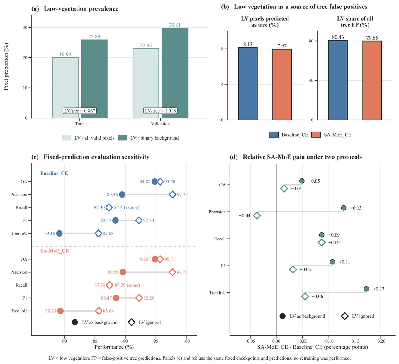
We utilized the Vaihingen dataset from the ISPRS 2D Semantic Labeling Challenge [40] to represent orthographic remote sensing imagery. Acquired over Vaihingen, Germany, this dataset contains 33 ultra-high-resolution (9 cm) orthophoto tiles with an average size of approximately 2500 × 2000 pixels, providing Near-Infrared (NIR), Red (R), and Green (G) spectral bands (stored in an IR-R-G false-color order). Compared with the RGB imagery in Cityscapes, the NIR-R-G composite provides additional vegetation-sensitive spectral information that may facilitate tree-canopy discrimination in orthographic imagery [41,42]. This advantage is shared by all models evaluated on ISPRS Vaihingen and therefore cannot account for the relative improvement of SA-MoE. Because the two datasets also differ in imaging geometry, spatial resolution, and task definition, their absolute accuracy values are not directly compared. Its pixel-level semantic labels cover six categories: impervious surfaces, buildings, low vegetation, trees, cars, and clutter/background. In the ISPRS taxonomy, low vegetation represents grass and other low-growing vegetation and is labeled separately from tree canopies [40]. We defined the ISPRS experiment as a binary tree canopy segmentation task. The tree class (ID = 3) was treated as the positive class, and all other classes, including low vegetation, were treated as negative. In this context, “background” means non target pixels in the binary task. The effect of this label definition is quantified in Appendix A Figure A3.

2.2. Evaluation Metrics

Our evaluation framework consists of specific metrics, including scale-aware recall and relaxed boundary-band overlap (R-Boundary), alongside global baseline metrics.

2.2.1. Scale-Aware Recall Based on Continuous Semantic Regions (CSR)

In both street-level and orthographic imagery, the long-tail scale distribution of target objects frequently biases global evaluation metrics toward large-scale features. This bias masks the model’s true detection performance on hard samples, such as distant or micro-scale vegetation. To mitigate this, we partitioned the ground-truth targets into four independent scales (extra-small (XS), small, mid, and large) based on connected-area quantiles (25%, 50%, and 75%). To account for the distinct imaging geometries and spatial resolutions of the two benchmarks, the 25th, 50th, and 75th percentiles were computed separately from the ground-truth CSR distribution of each evaluation set. These thresholds were used only for post-hoc stratified reporting and were applied identically to all evaluated models; they did not affect model training, hyperparameter selection, or prediction generation. The resulting XS, Small, Mid, and Large groups should therefore be interpreted as relative size strata within each dataset, rather than as absolute or directly comparable scale categories across datasets. We then calculated the recall for each scale independently to evaluate the model’s extraction capability for micro-objects within the long-tail distribution. The formula is as follows:

$${Recall}_{S_k}={\displaystyle \frac{{TP}_{S_k}}{{TP}_{S_k}+{FN}_{S_k}}}$$

where S_k represents the set of a specific scale. It is important to note that the scale category S_k is defined strictly by the Continuous Semantic Regions (CSR) of the ground truth (GT). Both ${TP}_{S_k}$ (correctly predicted vegetation pixels) and ${FN}_{S_k}$ (missed ground-truth vegetation pixels) are tallied entirely within these GT-defined boundaries.

2.2.2. Relaxed Boundary-Band Overlap Evaluation

To reduce the influence of boundary jitter in manual polygon delineations, we used a relaxed boundary-band overlap metric, termed R-Boundary. This metric is inspired by boundary-sensitive evaluation [43]. It measures the overlap between dilated predicted and ground-truth boundary bands. Intuitively, R-Boundary first converts both the predicted contour and the ground-truth contour into narrow tolerance bands, and then evaluates how well these two bands overlap. Thus, a predicted boundary is not severely penalized if it falls within a small tolerance range around the manually annotated boundary. This reduces the influence of minor annotation jitter.

$$R-Boundary={\displaystyle \frac{\left|B_{\theta }\left(P\right)\cap B_{\theta }\left(G\right)\right|}{\left|B_{\theta }\left(P\right)\cup B_{\theta }\left(G\right)\right|}}$$

where ${\mathrm{B}}_{\mathsf{\theta }}\left(\mathrm{P}\right)$ and ${\mathrm{B}}_{\mathsf{\theta }}\left(\mathrm{G}\right)$ denote the boundary bands obtained by dilating the predicted and ground-truth contours by θ pixels, respectively. In this study, θ was set to 3 pixels.

2.2.3. Global Baseline Metrics

We employed five widely adopted metrics in the semantic segmentation domain to assess global model accuracy: Overall Accuracy (OA), Precision, Global Recall, F1-Score, and mean Intersection over Union (mIoU). The formulas are as follows:

$$OA={\displaystyle \frac{TP+TN}{TP+TN+FP+FN}}$$

$$Precision={\displaystyle \frac{TP}{TP+FP}}$$

$$Recall={\displaystyle \frac{TP}{TP+FN}}$$

$$F1=2\times {\displaystyle \frac{Precision\times Recall}{Precision+Recall}}$$

The mIoU metric is calculated as:

$$mIoU={\displaystyle \frac{1}{k}}{\displaystyle \sum _{i=1}^k}{\displaystyle \frac{{TP}_i}{{TP}_i+{FP}_i+{FN}_i}}$$

where TP, TN, FP, and FN denote true positives, true negatives, false positives, and false negatives, respectively. The variable k in the mIoU formula indicates a segmentation task with k categories (in this study, k = 2, representing vegetation and background).

2.3. Scale-Aware Mixture of Experts Architecture

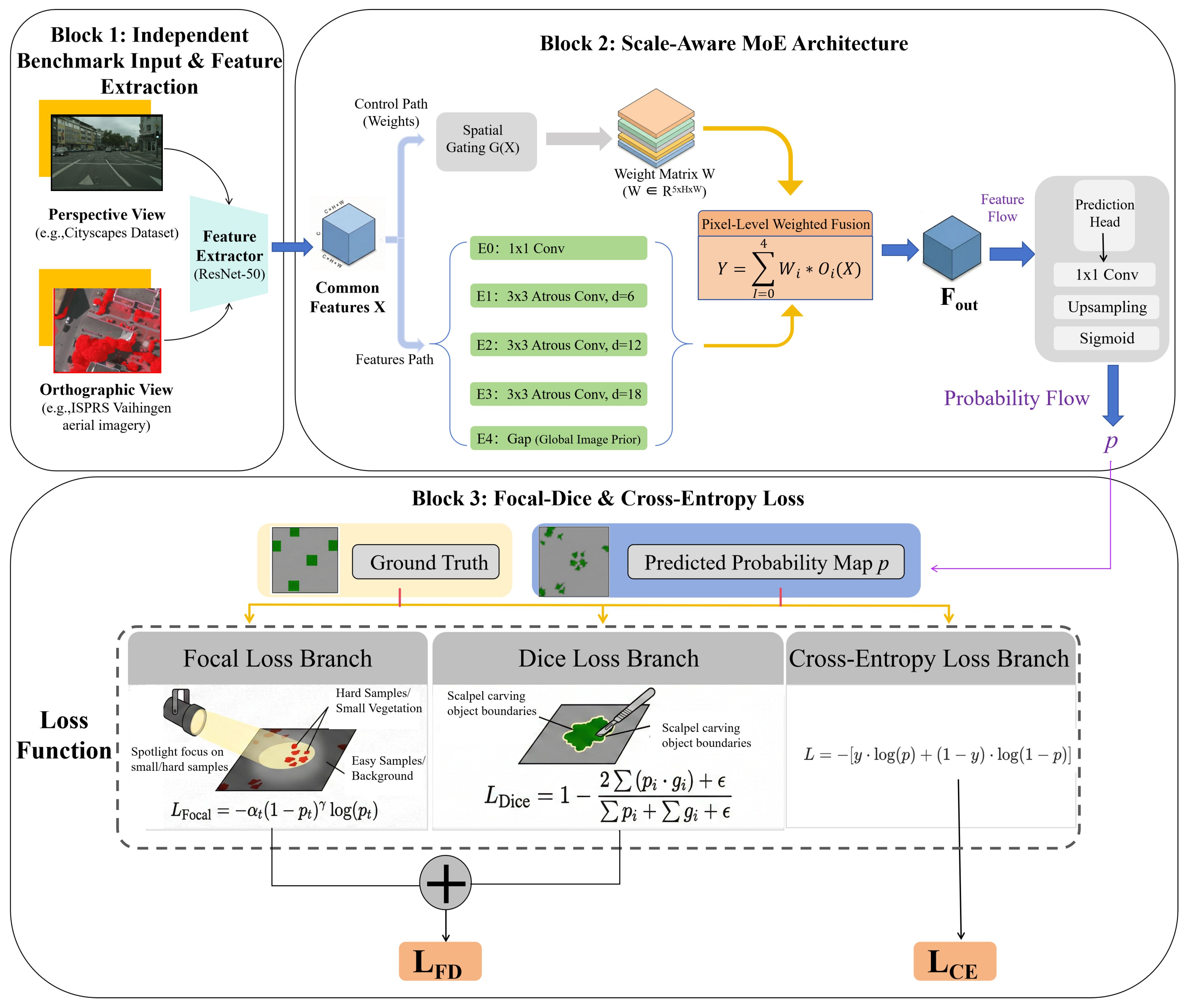
To address the long-tail effect of urban vegetation scales under two imaging views, as well as the “background engulfment” and texture washout (over-smoothing) defects inherent in the large receptive fields of traditional static scale-aggregation modules (e.g., ASPP) [17,18], we propose a fine-grained urban vegetation segmentation architecture based on a scale-aware mixture of experts and scene-specific optimization. The heterogeneous experts provide receptive-field options at each pixel. In street-level scenes, the gate can suppress large-dilation branches when they introduce excessive background around small targets. In orthographic scenes, it can shift weight toward smaller receptive fields in dense canopy regions, helping reduce sparse-sampling artifacts and preserve local texture. The selected features are then fused pixel by pixel. As illustrated in Figure 1, the same SA-MoE structure is evaluated separately on the street-level and orthographic benchmarks, performing adaptive scale perception and feature allocation through heterogeneous receptive-field experts and pixel-level dynamic routing for element-wise weighted fusion [23,32,33]. Its forward propagation and optimization design are deconstructed into the following core modules.

2.3.1. Spatial Gating Network with Temperature Polarization

Traditional semantic segmentation models rely on static weight concatenation, which inevitably absorbs excessive background noise. To enable dynamic, pixel-level selection of receptive fields, we designed a lightweight spatial gating network aimed at calculating the optimal receptive field weight for each individual pixel [33,44].

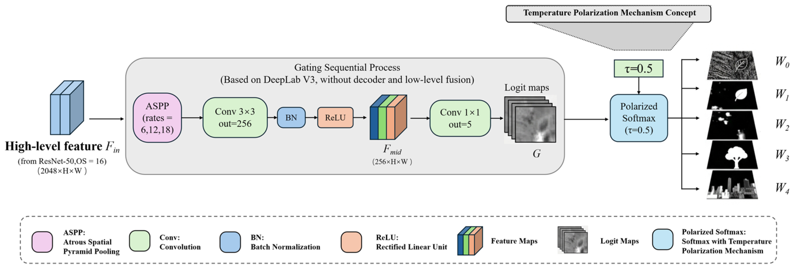
As shown in Figure 2, the gating network receives high-level feature maps from the ResNet-50 backbone with an output stride of 16. To enhance computational efficiency, its architecture adopts a lightweight bottleneck design. First, feature F_in undergoes spatial topological encoding through a 3 × 3 convolutional layer, which reduces the number of channels to 256. This is followed by spatial nonlinear modeling using batch normalization (BN) and ReLU activation. Finally, a 1 × 1 convolution layer maps the feature channels to the number of experts (five in this study), outputting an initial logit map that retains spatial positional information, denoted as $\mathrm{G}\in R^{5\times H\times \mathrm{W}}$.

If standard softmax is applied directly to normalize probabilities from the initial logit map, the resulting weight distribution across experts tends to be overly smooth. During subsequent weighted fusion, this often induces a “low-pass filtering” blur effect among different branch features. Therefore, before probability normalization, we introduce a temperature-scaling factor $\tau$. This process is formulated as:

$$W_i(p)=Polarized-Softmax(G_i(p),\tau )={\displaystyle \frac{exp\left(G_i\right(p)/\tau )}{{\sum }_{j=0}^{4}exp\left(G_j\right(p)/\tau )}}$$

where $G_i$ represents the score of the i-th layer of the initial logit map G, p denotes any given pixel, and ${\mathrm{W}}_{\mathrm{i}}\left(\mathrm{p}\right)$ represents the polarized weight of the i-th layer.

In this polarized gating network, when τ = 1.0, the network degrades to a standard Softmax. Conversely, if τ is too small, the gating distribution approaches hard routing (i.e., nearly one-hot). In this case, the gradients for the inactive experts become negligible, which may prevent them from being updated and leave them permanently inactive, thereby defeating the core purpose of the MoE architecture. Temperature scaling is widely used to control the sharpness and calibration of softmax probabilities [45], and sparse MoE studies have shown that routing sharpness, load balancing, and training stability are closely related to expert utilization [29,30,33]. In our setting, τ is therefore treated as an architectural routing-smoothness parameter acting on gating logits. Based on this consideration and the sensitivity analysis reported in Section 3.2 and the Appendix A Materials, τ was empirically set to 0.5 and then fixed for both datasets. This setting provides a practical balance between enhancing the distinction among expert weights and maintaining stable gradient propagation during training.

2.3.2. Mixture of Experts and Pixel-Level Fusion

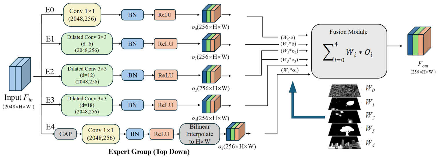
Concurrently with the generation of the polarized weight matrix by the spatial gating network, the generic features F_in are synchronously routed to a heterogeneous expert group comprising five parallel branches. As depicted in Figure 3, this expert group (E₀–E₄) contains five parallel branches. Among them, E₀ is a pixel-level expert utilizing a 1 × 1 convolution, designed to execute cross-channel deep feature fusion. To preserve a controlled comparison with the DeepLabV3 baseline, the three spatial experts retain the dilation rates used in its ASPP module: d = 6, 12, and 18 for E1, E2, and E3, respectively. This keeps the candidate receptive-field scales unchanged while replacing static concatenation with pixel-wise adaptive weighting, allowing the effect of the routing and fusion mechanism to be examined without simultaneously altering the dilation configuration. The progressively increasing rates provide distinct local, intermediate, and broader contextual candidates for the gating network. The differentiated routing patterns reported in Section 3.5 and Appendix A Figure A2 and

Table A2. Non-collapse check based on target-pixel routing weights.

Dataset	Spatial Expert Mass	Normalized Routing Entropy	E1 Activation Ratio W > 0.05	E2 Activation Ratio W > 0.05	E3 Activation Ratio W > 0.05
ISPRS Vaihingen	0.111	0.568	0.747	0.045	0.005
Cityscapes	0.470	0.803	0.991	0.938	0.895

further show that these branches receive scale- and view-dependent weights rather than acting as redundant parallel paths. The E4 expert applies global average pooling followed by a 1 × 1 convolution, batch normalization, and ReLU activation, to extract global contextual features. After undergoing BN and ReLU activation, these five branches output their respective local feature maps, denoted as ${\mathrm{O}}_{\mathrm{i}}\in R^{256\times H\times \mathrm{W}}(i\in \{0,1,2,3,4\left\}\right)$.

Once the local feature maps from the heterogeneous experts and the spatial polarized weight matrix from the gating network are obtained, the architecture performs pixel-level feature fusion. Specifically, an element-wise weighted sum is computed for any given spatial pixel p. The final aggregated Mixture-of-Experts feature, denoted as ${\mathrm{F}}_{\mathrm{out}}\in R^{256\times H\times \mathrm{W}}$, is formulated as follows:

$$F_{out}(p)={\displaystyle \sum _{i=0}^4}{W}_i\left(p\right)·O_i\left(p\right)$$

By replacing static concatenation with pixel-wise weighted summation, the architecture achieves adaptive aggregation of multi-scale features for vegetation segmentation under the two benchmark settings, effectively decoupling the process of receptive-field allocation from feature extraction.

2.3.3. Loss Function Design

We configured two loss functions in this study: Binary Cross-Entropy loss (CE loss, L_CE) and the joint Focal-Dice loss (L_FD). These two loss settings were evaluated separately and were not used simultaneously. In the subsequent ablation experiments, we independently assessed their respective performance improvements on the ISPRS and Cityscapes datasets. The specific formula for L_CE is:

$$L_{CE}=-{\displaystyle \frac{1}{N}}{\displaystyle \sum _{i=1}^N}\left[y_{i}log\right(P_i)+(1-y_i\left)log\right(1-P_i\left)\right]$$

where N denotes the total number of pixels in the image, and $y_i$ represents the ground-truth label of the i-th pixel. In this task, $y_i$= 1 when the pixel belongs to vegetation, and $y_i$ = 0 for the background. $P_i$ denotes the predicted probability that the pixel is vegetation, with $P_i$∈ (0, 1).

L_FD is defined as follows:

$$L_{FD}=L_{Focal}+L_{Dice}$$

Here, L_Focal is the Focal Loss [46] and L_Dice is the Dice Loss [47]. The formula for L_Focal is:

$$L_{Focal}=-{\alpha }_t{(1-p_t)}^{\gamma }log\left(p_t\right)$$

Here, ${\mathrm{P}}_{\mathrm{t}}$ represents the model’s predicted probability for the vegetation pixel, ${\alpha }_t$ is a weighting factor used to balance the ratio of positive and negative samples, and γ is the focusing parameter utilized to exponentially modulate the penalty applied to hard samples [46]. In this work, we set α = 0.25 and γ = 2, following the original Focal Loss setting [46]. The mean operation is applied over all pixels, which is equivalent to normalization by (N). The formula for L_Dice is:

$$L_{Dice}=1-{\displaystyle \frac{2{\sum }_{i=1}^N(p_i·g_i)+ϵ}{{\sum }_{i=1}^N{p}_i+{\sum }_{i=1}^N{g}_i+ϵ}}$$

where $p_i$ and $g_i$ represent the predicted probability and the ground-truth label distribution for pixel i, respectively, and $ϵ$ is a smoothing coefficient to prevent division by zero [47].

In this work, the two loss terms are equally weighted, following the balanced weighting strategy used in compound Dice–Focal-type losses such as Unified Focal Loss [48]. Since both terms are normalized and operate at a comparable scale, this setting allows stable joint optimization without introducing an additional loss-weighting hyperparameter.

2.3.4. Computation Mechanism of Dynamic Routing Weights

To quantitatively examine the routing behavior of the scale-aware MoE system across varying target scales, we established an evaluation framework to monitor the activation preferences of individual experts at distinct scales. We define the Absolute Routing Probability (ARP) as follows:

$$ARP(i,S_k)={\displaystyle \frac{1}{\left|S_k\right|}}\sum _{p\in S_k}{W}_i\left(p\right)$$

where $\left|{\mathrm{S}}_{\mathrm{k}}\right|$ denotes the total number of pixels belonging to the scale set ${\mathrm{S}}_{\mathrm{k}}$ (the concept of scale sets is introduced in Section 2.2.1), and for any given pixel, the normalization constraint ${\sum }_{\mathrm{i}=0}^4{W}_i\left(p\right)$ = 1 must be satisfied. This metric reflects the overall probability distribution of weight allocation among heterogeneous experts when the model processes vegetation of different scales.

Furthermore, to more precisely analyze the architecture’s selection logic among convolutional experts with varying dilation rates, we exclude the global-context expert (E₄) and the pixel-level expert (E₀), introducing the Relative Routing Probability (RRP) metric. The RRP for a spatial expert branch $i\in \{1,2,3\}$ is formulated as:

$$RRP(i,S_k)={\displaystyle \frac{ARP(i,S_k)}{{\sum }_{j=1}^{3}ARP(j,S_k)}}$$

Based on the RRP metric, we can quantitatively investigate how the relative weights of the scale experts vary with target scale.

3. Experiments and Results

In this section, we first detail the experimental setup. Subsequently, we present the procedures and results of the ablation studies to validate the efficacy of the proposed innovative modules, and to investigate the performance gains of distinct loss functions across datasets with different physical views. Finally, we conduct qualitative and quantitative comparisons with representative semantic segmentation baselines under a unified experimental protocol.

3.1. Implementation Details

The experiments were conducted on an Ubuntu operating system equipped with a single NVIDIA T4 GPU (16 GB), utilizing the PyTorch 2.9.0 deep learning framework. To accelerate model convergence, both our model and the CNN baselines employed an ImageNet-1K pre-trained ResNet-50 as the backbone network. Similarly, the Transformer-based models in the comparative experiments utilized their respective pre-trained weights. Input image dimensions were tailored to the dataset characteristics: training images from the Cityscapes and ISPRS datasets were randomly cropped to 768 × 768 and 512 × 512 pixels, respectively. The training process incorporated a unified dynamic data augmentation strategy, comprising random multi-scale scaling with a factor ranging from [0.5, 2.0], random cropping, and random horizontal flipping. The DeepLabV3 baseline uses a ResNet-50 backbone with output stride 16. The high-level 2048-channel features are processed by an ASPP module with dilation rates of 6, 12, and 18. No decoder or low-level feature fusion is used in this implementation.

The total number of training epochs was uniformly set to 50. The models were optimized using the AdamW optimizer (weight decay coefficient of 1 × 10⁻⁴). For CNN-based models, the optimizer was paired with a OneCycleLR scheduler (maximum learning rate of 0.001). Conversely, Transformer-based models were optimized using a constant learning rate of 0.0001 without an additional scheduler. Additionally, global gradient clipping with a threshold of 0.1 was applied. To enhance computational efficiency, Automatic Mixed Precision (AMP) was enabled during training, and the batch size was set to 12 for CNN-based models and 8 for Transformer-based models due to hardware VRAM constraints.

Statistical uncertainty in the principal ablation comparisons was assessed using paired bootstrap resampling of the evaluation predictions. We compared Baseline_FD with MoE_FD on Cityscapes and Baseline_CE with MoE_CE on ISPRS Vaihingen. A total of 10,000 paired resamples were drawn at the image level for Cityscapes and at the original image-area cluster level for ISPRS to account for dependence among adjacent patches. Ninety-five percent confidence intervals and two-sided p-values were computed for Global mIoU, XS Recall, and Mean Scale Recall, as reported in Appendix A 

Table A5. Paired bootstrap analysis of the principal performance differences between SA-MoE and the corresponding DeepLabV3 baseline on Cityscapes and ISPRS Vaihingen. Differences are reported in percentage points as SA-MoE minus the corresponding baseline. The 95% confidence intervals and two-sided p-values were obtained from 10,000 paired bootstrap resamples, using whole images as the resampling unit for Cityscapes and original image-area clusters for ISPRS Vaihingen. Values reported as p = 0.0000 in the computation output are presented as p < 0.0001.

Dataset	Metric	Difference	95% CI	p
Cityscapes	Global mIoU	+0.10 pp	[−0.31, 0.48]	0.7086
	XS Recall	+2.63 pp	[0.64, 4.78]	0.0108
	Mean Scale Recall	+1.49 pp	[0.78, 2.27]	<0.0001
ISPRS	Global mIoU	+0.63 pp	[−0.06, 1.28]	0.0690
	XS Recall	+5.09 pp	[3.42, 7.76]	<0.0001
	Mean Scale Recall	+3.53 pp	[2.88, 4.59]	<0.0001

.

3.2. Ablation Studies

To evaluate the proposed framework and examine the optimization biases of different loss functions across datasets with varying physical views, we first designed experiments to determine the temperature coefficient. Subsequently, we conducted ablation studies on the Cityscapes and ISPRS Vaihingen datasets. We selected the classic DeepLabV3 (ResNet50) as the baseline. When integrating the SA-MoE architecture, we retained the ResNet-50 backbone and replaced the static ASPP-based feature aggregation with the proposed SA-MoE module. In addition to the loss-level ablations reported in

Table 1. Quantitative results of the ablation study on the Cityscapes dataset. The best-performing result for each metric is highlighted in bold.

Model	Global		XS		Small		Mid		Large
	Boundary	mIoU	Boundary	Recall	Boundary	Recall	Boundary	Recall	Boundary	Recall
Baseline_CE	55.94%	89.39%	50.23%	53.64%	60.24%	82.47%	61.92%	93.39%	54.89%	96.16%
MoE_CE	57.22%	89.67%	51.69%	56.60%	61.83%	82.97%	62.52%	93.67%	55.72%	96.42%
Baseline_FD	56.41%	89.42%	50.60%	54.82%	60.45%	82.01%	61.95%	93.30%	55.05%	96.31%
MoE_FD (Best)	57.26%	89.52%	53.21%	57.45%	62.41%	84.34%	63.22%	93.90%	56.09%	96.72%

and

Table 2. Quantitative results of the ablation study on the ISPRS Vaihingen dataset. The best-performing result for each metric is highlighted in bold.

Model	Global		XS		Small		Mid		Large
	Boundary	mIoU	Boundary	Recall	Boundary	Recall	Boundary	Recall	Boundary	Recall
Baseline_CE	79.67%	79.69%	81.68%	68.90%	85.32%	82.64%	84.44%	87.46%	80.04%	90.33%
MoE_CE (Best)	79.96%	80.32%	80.76%	73.99%	84.85%	86.18%	84.46%	90.29%	80.93%	92.98%
Baseline_FD	79.02%	79.63%	79.01%	68.75%	83.63%	83.05%	83.86%	88.16%	79.81%	90.96%
MoE_FD	79.61%	80.20%	80.54%	72.88%	84.86%	86.42%	83.87%	90.11%	80.46%	92.73%

, we further conducted a module-wise ablation to isolate the contribution of each introduced component, including heterogeneous experts, dynamic routing, temperature polarization, and the complete expert group. The detailed results are provided in Appendix A 

Table A4. Module-wise ablation results of the proposed SA-MoE architecture on the Cityscapes and ISPRS Vaihingen datasets. The best-performing result for each metric is highlighted in bold. “√” indicates that the corresponding component is included, whereas “×” indicates that it is not included.

Dataset	Variant	Heterogeneous Experts	Dynamic Routing	τ Polarization	Complete Expert Group	Global mIoU (%)	XS Recall (%)	Small Recall (%)	Mean Scale Recall (%)
Cityscapes	DeepLabV3 baseline	×	×	×	×	89.42	54.82	82.01	81.61
	Static-Expert Fusion	√	×	×	√	89.19	54.93	81.76	81.46
	Spatial-only MoE	partial	√	√	×	89.41	55.06	82.13	81.71
	Dynamic MoE, τ = 1.0	√	√	×	√	89.44	55.36	82.53	81.78
	Full SA-MoE, τ = 0.5	√	√	√	√	89.52	57.45	84.34	83.10
ISPRS Vaihingen	DeepLabV3 baseline	×	×	×	×	79.69	68.90	82.64	82.33
	Static-Expert Fusion	√	×	×	√	78.29	68.05	82.93	82.10
	Spatial-only MoE	partial	√	√	×	78.06	66.97	81.82	81.33
	Dynamic MoE, τ = 1.0	√	√	×	√	78.71	69.16	83.15	82.65
	Full SA-MoE, τ = 0.5	√	√	√	√	80.32	73.99	86.18	85.86

.

(1)

Selection of the Temperature Coefficient $\tau$

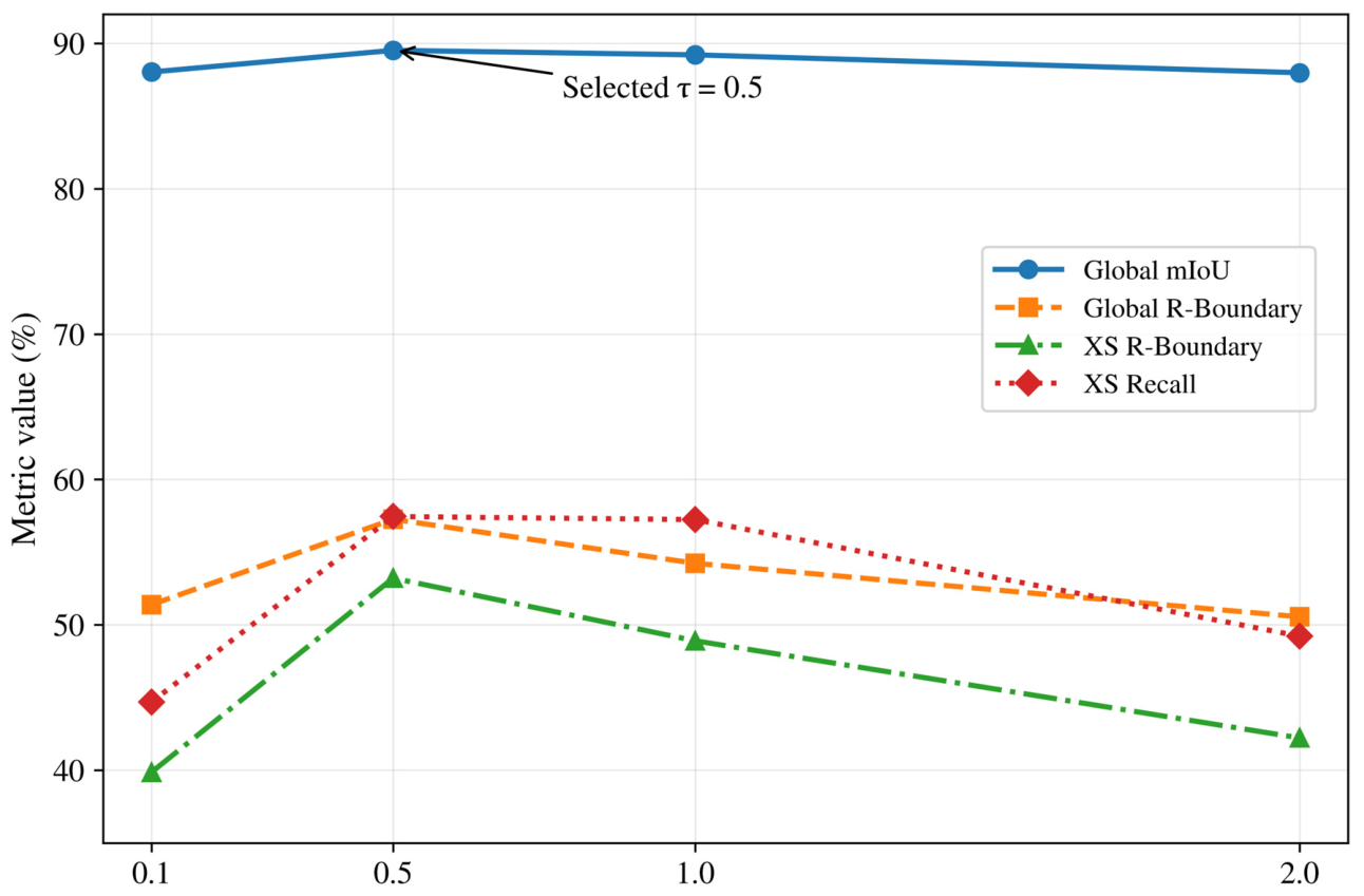
First, using the Cityscapes dataset as a representative case, we evaluated the influence of the temperature coefficient τ in the polarized gating network. In the initial sensitivity analysis, four candidate values, τ = 0.1, 0.5, 1.0, and 2.0, were tested using Global mIoU, Global R-Boundary, XS R-Boundary, and XS Recall as the main indicators. The results indicated that τ = 0.5 provided strong overall performance among the initially tested candidates (Figure 4).

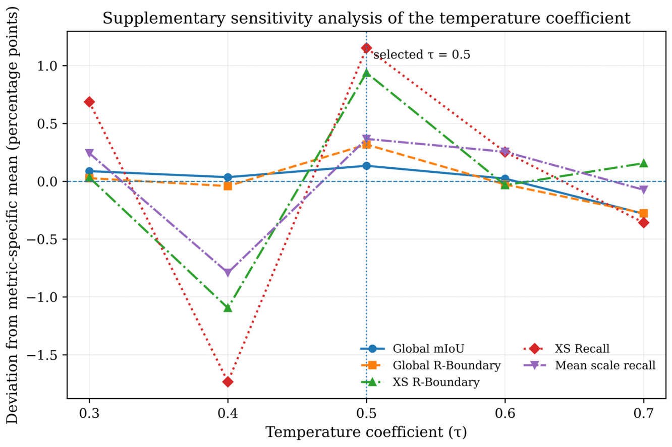
To further examine the local sensitivity around this value, we additionally conducted a denser supplementary analysis using τ = 0.3, 0.4, 0.5, 0.6, and 0.7. As shown in Appendix A Figure A1 and Appendix A 

Table A1. Supplementary sensitivity analysis of the temperature coefficient τ. The best-performing result for each metric is highlighted in bold.

τ	Global mIoU (%)	Global R-Boundary (%)	XS R-Boundary (%)	XS Recall (%)	Mean Scale Recall (%)
0.3	88.79	60.97	48.54	53.90	81.23
0.4	88.74	60.90	47.41	51.48	80.20
0.5	88.84	61.26	49.44	54.36	81.35
0.6	88.73	60.91	48.47	53.46	81.24
0.7	88.42	60.66	48.66	52.85	80.91

, τ = 0.5 achieved the best overall balance among the tested candidates, with the highest Global mIoU, Global R-Boundary, XS R-Boundary, XS Recall, and Mean Scale Recall. Because τ acts on the gating distribution, we used τ = 0.5 as a fixed architectural setting in both datasets for controlled comparison and to avoid additional dataset-specific tuning.

(2)

Ablation Study on the Street-Level Dataset

To validate the effectiveness of the proposed SA-MoE architecture and the FD loss function tailored for perspective street-level datasets, we performed an ablation study on the Cityscapes dataset, with results summarized in Table 1. The quantitative results show that the introduction of the MoE architecture improved the scale-aware boundary and recall metrics, with clearer gains for XS and small-scale vegetation. Concurrently, the gains tended to be larger for smaller vegetation regions: under both CE and FD loss functions, the MoE architecture improved the recall for XS scales by 2.96 and 2.63 percentage points, respectively, and for the Small group by 0.50 and 2.33 percentage points. Conversely, the improvements for mid and large scales remained marginal (within 0.3 and 0.6 percentage points). Furthermore, a horizontal comparison demonstrates that employing the FD loss further improved R-Boundary scores and recall across scales, indicating that the synergy between the SA-MoE architecture and the FD loss function can further exploit the segmentation potential of street-level datasets. The paired bootstrap analysis showed that the improvements in XS Recall and Mean Scale Recall were statistically supported, whereas the small difference in Global mIoU was not statistically significant (Appendix A Table A5).

(3)

Ablation Study on the Aerial Dataset

To further examine whether the same SA-MoE design remains effective in the orthographic benchmark, we conducted an identical ablation study on the ISPRS dataset, as shown in Table 2. The quantitative data indicate that SA-MoE provides consistent recall gains under the orthographic aerial view, reaffirming the negative correlation between scale and accuracy gains observed in the street-level experiment. Under the CE loss function, the MoE module achieved an increase of 5.09 percentage points in recall at the XS scale, while the recall gains for mid-to-large scale targets hovered between 2.6 and 2.8 percentage points.

A noteworthy observation is the differential performance of the loss functions across the two benchmark settings. Unlike the street-level dataset, where the FD loss function comprehensively improved scale-aware accuracy, the MoE model equipped with the CE loss achieved the highest point estimates for most reported metrics under this setting in the aerial dataset. For instance, its XS-scale recall outperformed the FD-equipped MoE model by 1.11 percentage points. This phenomenon suggests that artificial label noise, such as boundary misalignments and positional shifts inherent in orthographic remote sensing scenarios, may negatively affect the FD loss by encouraging the learning of inaccurate boundaries under the current parameter settings. Conversely, the CE loss function, grounded in independent pixel-wise evaluation, exerts a superior smoothing effect on such noise, making it relatively more robust in this specific experimental setting [49]. In this study, we did not perform extensive hyperparameter tuning for the FD loss, and the parameters were kept fixed for fair comparison. All FD experiments used the same fixed configuration of α = 0.25 and γ = 2, without dataset-specific tuning. Therefore, the comparison between CE and FD in this study should be interpreted under this predefined setting. The paired cluster bootstrap analysis likewise supported the improvements in XS Recall and Mean Scale Recall, while the difference in Global mIoU did not reach statistical significance (Appendix A Table A5).

(4)

Module-wise Ablation of the SA-MoE Components

The module-wise ablation results in Appendix A Table A4 show that static expert fusion alone does not consistently improve performance, indicating that simply increasing the number of parallel branches is insufficient. Introducing dynamic routing improves scale-aware recall compared with static fusion, while the full SA-MoE configuration with τ = 0.5 achieves the strongest XS and small-scale recall, especially on the ISPRS Vaihingen dataset. These results support that the performance gain mainly comes from adaptive expert allocation and the complete scale-aware routing design.

3.3. Comparative Experiments and Results

Building upon the ablation studies, we conducted comparisons with representative algorithms covering several mainstream architecture families: fully convolutional and context-aggregation models (U-Net [50] and PSPNet [51]), spatial/channel attention-based models (MANet [26]), convolutional-attention/large-kernel models (SegNeXt-Tiny [22]), and Transformer-based models (SegFormer [27] and Swin-UPerNet [28]). To isolate the effect of network architecture during comparative evaluation, all models were trained using the dataset-specific loss functions identified in Section 3.2 (FD for Cityscapes and CE for ISPRS). It should be noted that Table 1 and Table 2 establish the overall architectural contribution of SA-MoE under the dataset-specific loss settings, while Appendix A Table A4 further isolates the role of each introduced module. The purpose of this comparison is a controlled sanity check under a unified protocol rather than a claim to reproduce every model’s best public benchmark score. Public benchmark scores, which are usually reported for the original multi-class segmentation tasks, are not directly comparable with our binary vegetation/tree segmentation setting because of differences in class definitions, input cropping, data partitioning, and evaluation metrics. To address recent convolutional-attention and large-kernel segmentation designs, SegNeXt-Tiny was additionally evaluated and reported in the appendix comparison tables (Appendix A 

Table A3. Comparison of SA-MoE with SegNeXt-Tiny, a representative large-kernel convolutional-attention segmentation model, on the Cityscapes and ISPRS Vaihingen benchmarks. The best-performing result for each metric is highlighted in bold.

Dataset and Model		Model Complexity and Efficiency			Accuracy Metrics
Dataset	Model	Params (M)	GFLOPs	FPS	OA	F1	mIoU	Global R-Boundary	XS Recall	Mean Scale Recall
Cityscapes	MoE_FD	44.81	1184.29	3.2	98.31%	94.59%	89.52%	57.26%	57.45%	83.10%
	SegNeXt-Tiny	4.56	115.84	5.26	98.22%	94.15%	88.96%	51.93%	52.32%	80.69%
ISPRS Vaihingen	MoE_CE	44.81	148.04	23.2	95.06%	90.28%	80.32%	79.96%	73.99%	85.86%
	SegNeXt-Tiny	4.56	14.48	60.82	94.72%	88.28%	79.01%	77.89%	68.90%	82.83%

). The results show that SegNeXt-Tiny is substantially lighter and faster, whereas SA-MoE retains higher global accuracy and scale-aware recall under the same local protocol.

(1)

Computational Efficiency

To assess the feasibility of model deployment in real-world scenarios,

Table 3. Comparison of computational complexity, model parameters, and inference efficiency across different models.

Model	Backbone	Params (M)	ISPRS Dataset		CityScapes Dataset
			GFLOPs	FPS	GFLOPs	FPS
U-Net	ResNet50	32.52	85.73	36.4	685.84	4.6
PSPNet	ResNet50	24.31	23.72	93.6	189.72	11.4
MANet	ResNet50	147.44	149.3	19.2	1194.45	3
SegFormer	MiT-b2	27.35	113.43	19.8	907.41	1.3
Swin-UPerNet	Tiny	59.83	471.77	9.5	3756.32	1.2
DeepLabV3	ResNet50	40.35	138.91	24.4	1111.24	3.3
SA-MoE (Ours)	ResNet50	44.81	148.04	23.2	1184.29	3.2

reports the parameters (Params), computational complexity (GFLOPs), and inference frame rates (FPS) for each model. Because computational load and frame rate depend on input resolution, measurements were conducted at two input sizes: the ISPRS dataset (512 × 512) and the Cityscapes dataset (2048 × 1024).

The results reveal that after integrating the dynamic routing mechanism of the mixture of experts, SA-MoE added only 4.46 M parameters relative to the baseline (DeepLabV3), indicating limited computational overhead. Its inference rates were 23.2 FPS for ISPRS and 3.2 FPS for Cityscapes. For high-resolution Cityscapes images, Swin-UPerNet required 3756.32 GFLOPs and ran at 1.2 FPS. By contrast, SA-MoE required approximately one-third of this computation, providing a favorable balance between computational efficiency and segmentation accuracy.

All parameter counts were obtained using the same procedure. Although MANet also adopts ResNet-50 as its backbone, its relatively large parameter count mainly arises from the attention-based decoder and multi-scale feature-fusion modules, which introduce additional independently parameterized convolutional and attention blocks.

(2)

Street-Level Dataset

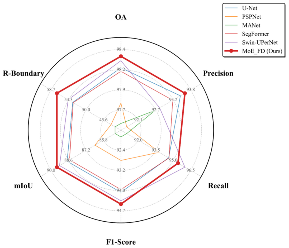
The six-dimensional radar chart comparing global performance on the street-level dataset is presented in Figure 5, with the fine-grained scale-specific evaluation detailed in

Table 4. Scale-aware quantitative evaluation of boundary precision (R-Boundary) and recall across different models on the Cityscapes dataset.

Model	XS		Small		Mid		Large
	Boundary	Recall	Boundary	Recall	Boundary	Recall	Boundary	Recall
U-Net (ResNet-50)	43.53%	51.08%	57.29%	80.39%	58.52%	92.51%	51.09%	95.91%
PSPNet (ResNet-50)	39.79%	51.47%	48.69%	79.85%	49.38%	90.96%	44.39%	95.18%
MANet (ResNet-50)	32.67%	42.24%	45.86%	74.36%	46.05%	87.32%	40.63%	92.74%
SegFormer (MiT-b2)	48.40%	57.20%	57.42%	82.74%	57.99%	92.28%	51.10%	95.82%
Swin-UPerNet (Tiny)	52.59%	61.77%	61.37%	86.42%	61.33%	93.90%	53.52%	96.99%
MoE_FD (Ours)	53.21%	57.45%	62.41%	84.34%	63.22%	93.90%	56.09%	96.72%

. The radar chart illustrates the competitive performance of our proposed MoE_FD model across global metrics. Specifically, the OA, Precision, Recall, F1-Score, and mIoU of MoE_FD reached 98.31%, 93.59%, 95.62%, 94.59%, and 89.52%, respectively. The global OA and F1-Score of MoE_FD were slightly higher than those of the other models, whereas its Recall was marginally lower than that of the Swin-UPerNet (Tiny) model. The traditional CNN models all achieved mIoU values below 87% in the perspective street scenes. The self-attention-based Swin-UPerNet (Tiny) achieved the highest global recall (95.96%), though with a comparatively lower precision (92.80%).

Table 4 shows that the proposed MoE_FD model achieves the highest R-Boundary precision across all scales, reaching 53.21% and 62.41% at the XS and Small scales, respectively. This corresponds to an improvement of nearly 5 percentage points over SegFormer (MiT-b2) (48.40% and 57.42%), which performs strongly among the compared baselines. In terms of recall, the proposed model is comparable to Swin-UPerNet (Tiny) at the mid scale, but slightly lower at the XS, small, and large scales (Table 4). Nevertheless, it still outperforms the other CNN-based models while maintaining higher computational efficiency. Overall, the results indicate that the proposed model improves R-Boundary precision while retaining competitive recall, offering a favorable trade-off between accuracy and efficiency.

(3)

Aerial Dataset

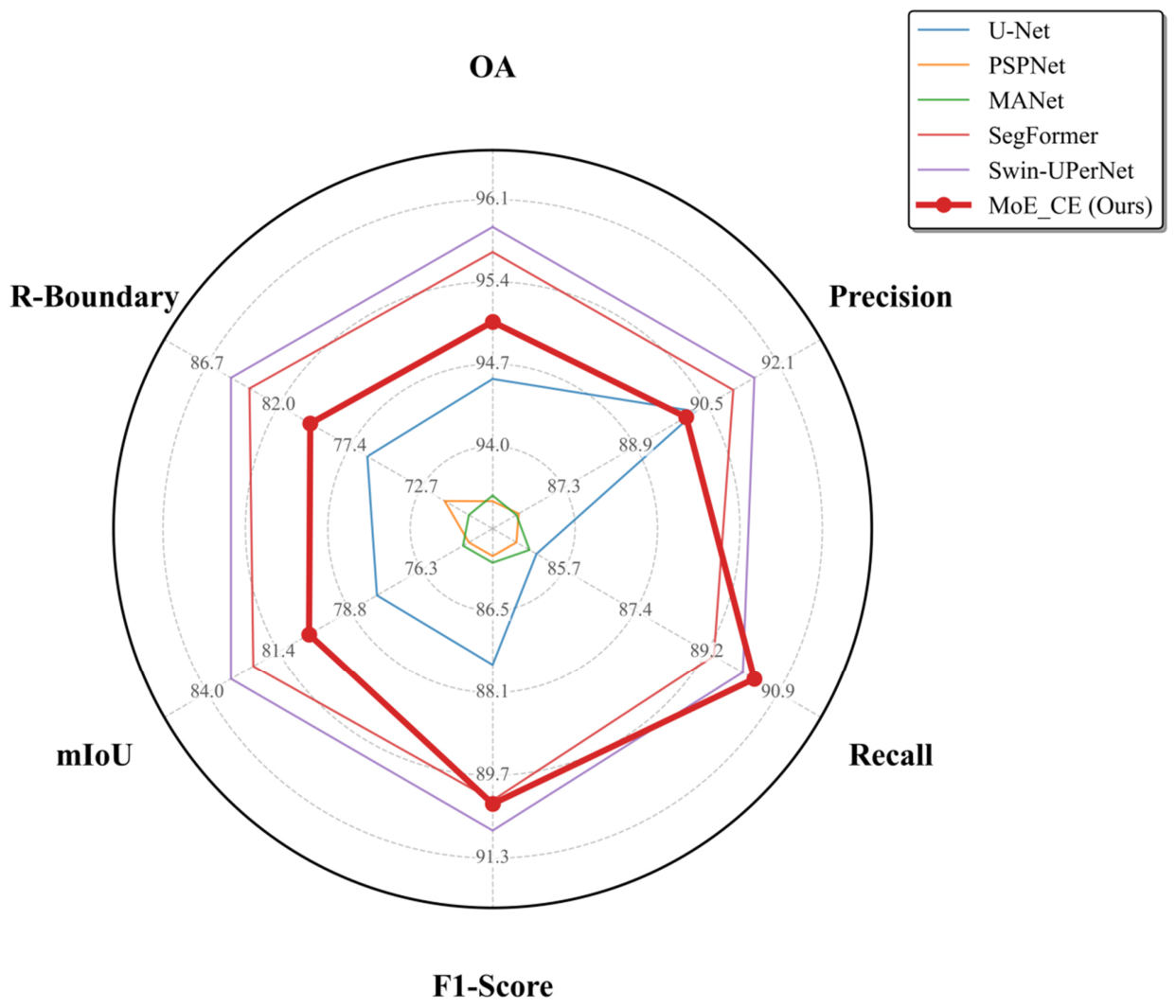
The six-dimensional radar chart and scale-specific accuracy evaluation table for the aerial dataset are displayed in Figure 6 and

Table 5. Scale-aware quantitative evaluation of boundary precision (R-Boundary) and recall across different models on the ISPRS Vaihingen dataset. The best-performing result for each metric is highlighted in bold.

Model	XS		Small		Mid		Large
	Boundary	Recall	Boundary	Recall	Boundary	Recall	Boundary	Recall
U-Net (ResNet-50)	70.55%	57.87%	80.01%	78.61%	81.41%	85.35%	77.21%	88.74%
PSPNet (ResNet-50)	73.29%	62.91%	78.19%	79.63%	76.95%	85.38%	70.89%	87.27%
MANet (ResNet-50)	64.86%	58.59%	73.15%	78.19%	75.58%	86.02%	70.88%	88.25%
SegFormer (MiT-b2)	85.11%	70.60%	89.08%	86.03%	87.10%	89.08%	83.35%	91.90%
Swin-UPerNet (Tiny)	85.24%	70.78%	90.15%	86.27%	88.17%	89.61%	85.17%	92.80%
MoE_CE (Ours)	80.76%	73.99%	84.85%	86.28%	84.46%	90.29%	80.93%	92.98%

. For global metrics, the OA, Precision, Recall, F1-Score, mIoU, and R-Boundary of MoE_CE reached 95.06%, 90.06%, 90.32%, 90.28%, 80.32%, and 79.96%, respectively. Its comparison with other mainstream models exhibits a diametrically opposite trend to that of the street-level dataset, achieving the top score solely in Recall, while the remaining global metrics trailed the two Transformer-based architectures. This suggests that in orthographic aerial datasets, the self-attention mechanisms of Transformer architectures hold a distinct advantage in capturing global contexts and fitting macroscopic boundaries; nonetheless, our improved CNN-based SA-MoE architecture achieved the highest recall. Appendix A Figure A3 examines the influence of the low-vegetation label treatment in the ISPRS experiment. Low vegetation represents 22.93% of the evaluation pixels and contributes approximately 80% of the false-positive tree predictions. Excluding these pixels from evaluation increases the Precision, F1-score, and Tree IoU of both models. SA-MoE_CE still achieves slightly higher OA, Recall, F1-score, and Tree IoU, and the difference in Precision is only 0.04 percentage points. The analysis is based on fixed predictions and does not involve model retraining.

In the scale-specific accuracy evaluation, the MoE_CE model achieved the highest Recall across all four scales, notably outperforming the runner-up by 3.21 percentage points at the XS scale. However, for the R-Boundary metric, our model lagged behind the best-performing Swin-UPerNet (Tiny) model by approximately 4 to 5 percentage points across all scales. This result highlights the stronger boundary delineation of Transformer architectures, whereas SA-MoE reduces omissions of micro-scale and fragmented vegetation through dynamic routing and receptive-field allocation. This trade-off reflects the different inductive biases of the two model families. The dynamic routing mechanism of SA-MoE tends to allocate more suitable receptive-field experts to fragmented or small vegetation regions, thereby reducing missed detections and improving recall. In contrast, Transformer-based models benefit from long-range self-attention and are therefore better able to preserve global shape consistency and boundary continuity, especially in orthographic scenes with continuous canopy structures.

3.4. Qualitative Visual Analysis

(1)

Ablation Studies

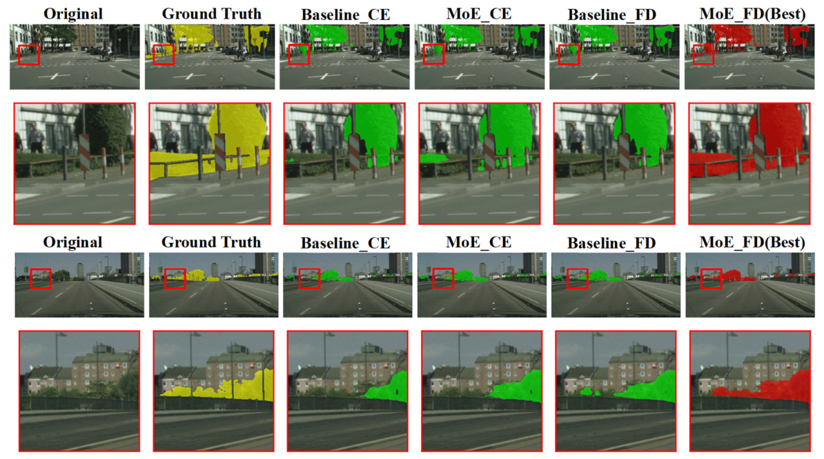
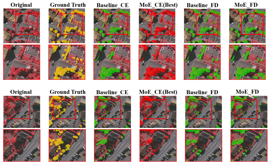
To illustrate the visual behavior of the proposed SA-MoE architecture, we visualized the vegetation segmentation results on both datasets, as depicted in Figure 7 and Figure 8. The results in Figure 7 suggest that the integration of the MoE architecture improves the identification of distant, micro-scale objects, including vegetation that the baseline model overlooked. The FD loss further enhances this tendency for the street-level benchmark. Figure 8 shows that the MoE architecture improves the segmentation of small-scale, disconnected vegetation and reduces omissions in several representative regions. Comparing the visualizations of the two loss functions within the MoE architecture, the CE loss appears more stable for small-scale vegetation in aerial imagery, which is consistent with the quantitative trends in the ablation studies.

(2)

Comparative Experiments

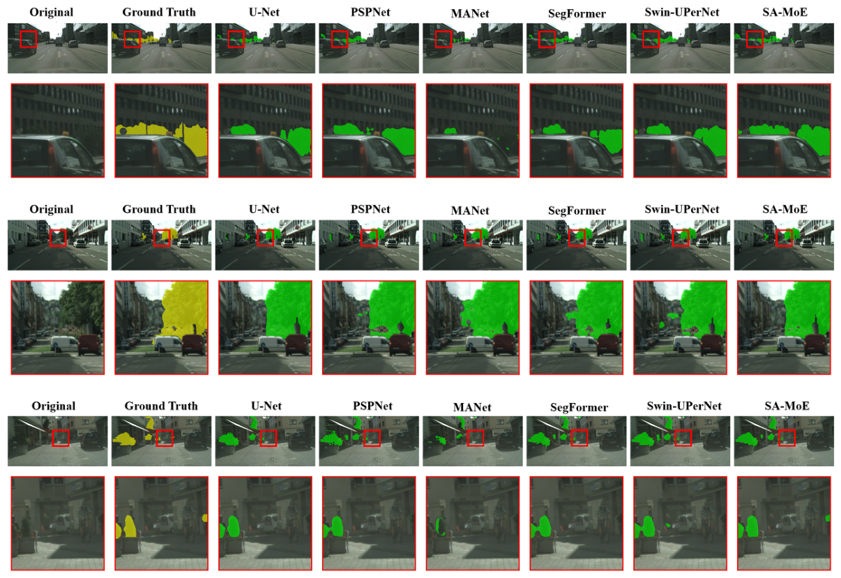
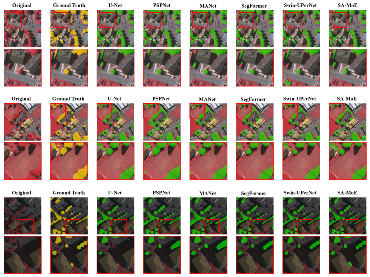
Expanding upon the ablation studies, we conducted qualitative visual comparisons between the selected SA-MoE configurations and representative semantic segmentation architectures. Figure 9 and Figure 10 illustrate the visual performance of these models under the two independent imaging views.

A cross-model analysis of Figure 7, Figure 8, Figure 9 and Figure 10 further reveals several typical failure modes of different architectures under scale variations across the two imaging views. Models relying on traditional deep convolutions and spatial pooling (U-Net (ResNet-50), PSPNet (ResNet-50), and MANet (ResNet-50)) tend to lose fine-grained spatial details during successive downsampling operations. As a result, they show conspicuous omissions in distant street-level vegetation and fragmented aerial canopies, together with false positives in complex background regions and overly smooth predicted boundaries. In contrast, Transformer-based models (SegFormer (MiT-b2) and Swin-UPerNet (Tiny)) benefit from global self-attention and perform better in maintaining the connectivity, structural integrity, and boundary continuity of macro-scale vegetation. However, they still exhibit noticeable omissions and misclassifications when dealing with scattered XS targets. These visual comparisons indicate that SA-MoE mainly improves the detection of small and fragmented vegetation regions, although its boundary continuity in orthographic scenes remains weaker than that of the strongest Transformer-based models.

Overall, the proposed SA-MoE architecture provides a favorable visual trade-off in both benchmark settings, with clearer recall advantages for small-scale targets while still showing room for improvement in boundary continuity compared with the strongest Transformer-based models.

3.5. Visualization and Analysis of Dynamic Routing

To examine whether the scale-aware architecture adaptively allocates experts according to vegetation scale, we extracted the gating weights during forward propagation and visualized them using the ARP and RRP frameworks defined in Section 2.3.4. We analyzed the routing distributions on the test sets independently for the perspective street-level dataset (Cityscapes) and the orthographic remote sensing dataset (ISPRS). This analysis provides model-side evidence for comparing expert allocation patterns across datasets with distinct physical views.

(1)

Perspective Street-Level Dataset

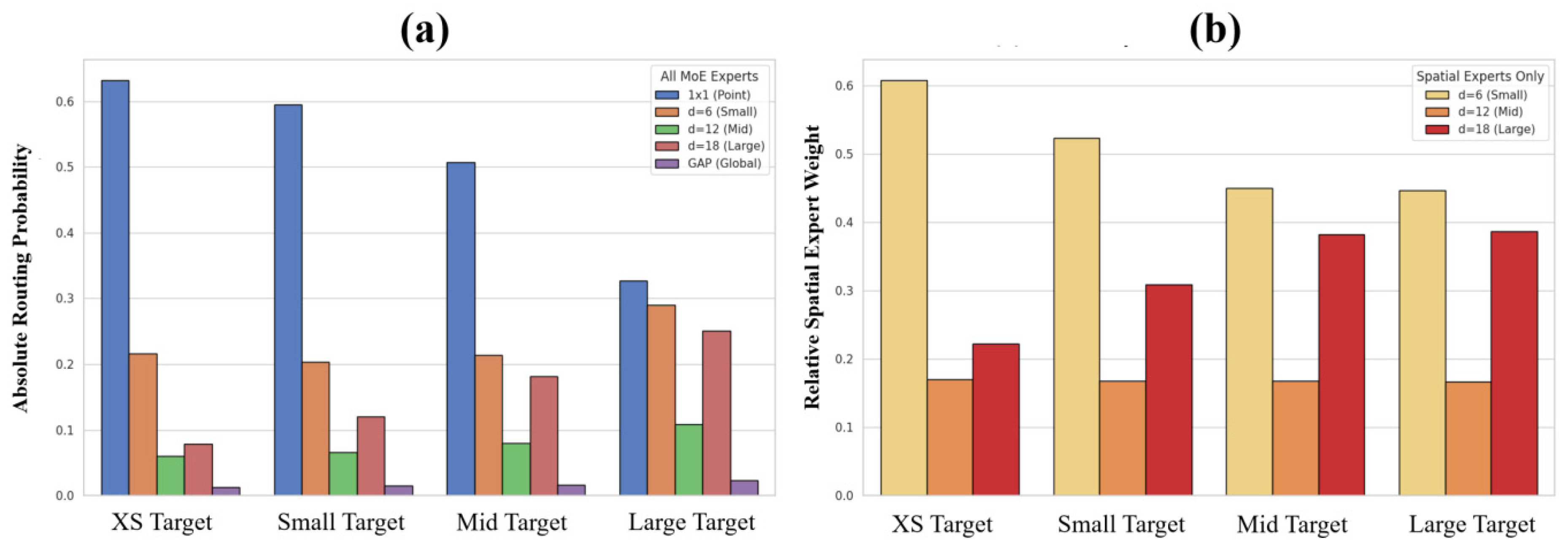
In perspective street-level scenarios, the dynamic routing mechanism of our model showed a positive association with target scale. As shown by the absolute distribution in Figure 11a, the pixel-level 1 × 1 convolution expert (E0) received the highest absolute weight at all scales; however, its weight decreased as target size increased (from 0.631 for XS targets to 0.326 for Large targets). A closer inspection of the relative routing weights of the spatial scale experts (Figure 11b) shows that for XS targets, the small-receptive-field expert received the highest relative weight (0.607), whereas the large-receptive-field expert received 0.222. As target size increased, the relative weight of the large-receptive-field expert increased to 0.386 for large targets, while the small-receptive-field expert decreased to 0.446. Meanwhile, the absolute weight of the mid-receptive-field expert increased slightly with scale, though its relative weight remained stable. These observations suggest that under perspective-induced scale variation, the spatial experts show a scale-dependent routing tendency. Larger vegetation regions tend to receive relatively higher contributions from large-receptive-field experts for contextual modeling, whereas XS targets rely more on small-receptive-field experts to reduce background interference.

(2)

Orthographic Aerial Dataset

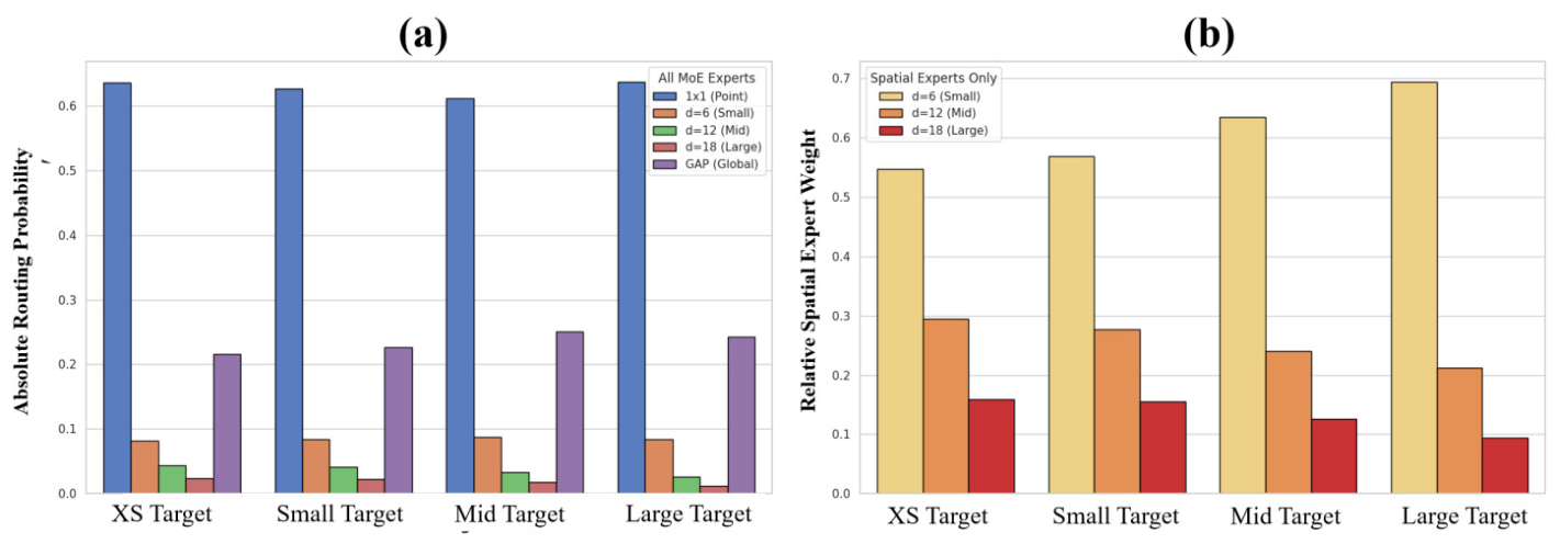
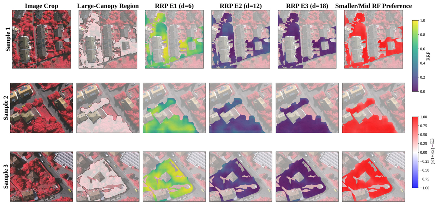
Under orthographic aerial scenarios, the routing behavior followed a different pattern from that observed in the street-level dataset. As shown in Figure 12a, the pixel-level expert E0 and the global-context expert E4 received relatively high absolute routing weights, suggesting that they provided the main baseline representation and global contextual support. To better understand the spatial experts, we further examined the relative routing probabilities among E1–E3. As shown in Figure 12b, the relative weight of the large-dilation expert E3 decreased as the vegetation scale increased, whereas E1 maintained the highest relative routing probability among the spatial experts. For large-scale canopy regions, the RRP of E1 reached 0.763, while that of E3 decreased to 0.067. We therefore interpret this pattern as a relative routing shift away from the large-dilation expert toward smaller-to-middle receptive-field experts, rather than as a strict one-to-one matching between object size and receptive-field size.

To provide direct model-side evidence for this interpretation, we added routing-weight visualizations for representative large-canopy samples in Appendix A Figure A2. The visualization shows that E3 remains weak within large-canopy regions, while the relative routing weights are mainly assigned to E1 and, to a lesser extent, E2. In addition, we conducted a non-collapse check based on the target-pixel routing weights, as summarized in Appendix A Table A2. In the orthographic dataset, E1 showed an activation ratio of 0.747 under the threshold W > 0.05, and the normalized routing entropy was 0.568. These results suggest that the observed pattern is not a complete collapse of the spatial expert group, but rather a suppression of the large-dilation expert E3 and a relative shift toward E1/E2.

4. Discussion

4.1. Performance Under Two Imaging Views and Scene-Specific Optimization

The proposed SA-MoE architecture shows stable and adaptive segmentation performance in both perspective street-level and orthographic aerial views. Compared with the representative baselines evaluated under the same experimental protocol, the SA-MoE-based model achieved competitive global performance on the street-level dataset. On the aerial dataset, it maintained competitive global metrics and achieved the best recall across scales, especially at the XS scale.

Furthermore, this study analyzes the relationship between optimization objectives (loss functions), dataset imaging characteristics, and annotation noise across the two benchmark settings. While selecting specific loss functions for distinct datasets is a common empirical practice, our results suggest why divergent physical views may favor different optimization strategies. In perspective street-level imagery, the scale imbalance of vegetation and the surge of hard samples demand robust local focusing capabilities from the loss function [11,36,46]. Using the FD loss improved several boundary-related and scale-aware recall metrics of SA-MoE on Cityscapes. Conversely, in orthographic aerial imagery characterized by artificial label noise [37,49], the CE loss function exhibits stronger robustness in this experimental setting. These observations suggest that optimization strategies should be selected with attention to the physical properties and noise characteristics of the scene, rather than relying on a universal objective [52].

4.2. Receptive Field Inversion Pattern and Interpretation

The dynamic routing visualization in Section 3.5 further illustrates how the proposed SA-MoE architecture responds to datasets from two imaging views. In perspective street-level scenes represented by the Cityscapes dataset, the expert-weight allocation pattern is consistent with the scale variation caused by perspective projection. For near-field targets occupying a large field of view, the model tends to elevate the weights of large-scale experts to capture global context [18]. Conversely, for distant small targets affected by severe perspective distortion, the architecture increases the weights of small-scale experts to reduce omissions. This routing behavior is consistent with the findings of Hamaguchi et al. [53]. Their results suggest that, when processing micro-targets, sparse convolution kernels with large dilation rates may fail to aggregate local features effectively and may introduce redundant background elements (e.g., buildings and sky). By assigning higher relative weights to the pixel-level expert and small-dilation experts, SA-MoE may reduce background interference at the receptive-field allocation stage [23,53]. Similar sparse-sampling effects may also occur locally in Cityscapes; however, the aggregate routing statistics did not show a corresponding suppression of the large-dilation expert, and we therefore do not interpret such effects as a dominant factor in the Cityscapes routing pattern.

In orthographic remote sensing scenarios represented by the ISPRS dataset, the model shows a counter-intuitive routing pattern that we refer to as “receptive field inversion”. Specifically, when processing large-scale vegetation, the architecture assigns lower relative weights to large-dilation experts and relies more on small-receptive-field experts [19,23,54]. We hypothesize that this may be related to the high local variance and high-frequency texture characteristics of very high-resolution orthographic canopies described in classic scale theory [55]. In addition, CNNs are known to exhibit texture bias during feature extraction [56], and large-dilation convolutions can produce gridding artifacts in dense prediction tasks [19,54]. One possible explanation is therefore that, for large canopy regions with dense local texture, excessive sparse sampling may weaken useful local texture cues, whereas smaller receptive fields preserve more local continuity. Boundary regions are known to benefit from high-resolution, spatially detailed processing in semantic segmentation [43,57], which may partly contribute to the observed preference for smaller receptive fields. However, Appendix A Figure A2 shows that the E1/E2 preference also extends across substantial canopy interiors rather than being confined to narrow boundary bands. We therefore consider boundary localization and texture preservation as non-exclusive hypotheses. Under this interpretation, the observed routing shift may help reduce texture washout while retaining some contextual support. However, the current evidence is based on routing statistics and visualizations rather than direct causal ablation, so this mechanism should be regarded as a hypothesis for future testing.

4.3. Limitations and Future Work

This study still presents certain limitations. First, the current experiments are based on well-annotated benchmark datasets mainly representing European urban environments. Therefore, the geographic generalizability of SA-MoE to regions with substantially different vegetation structures, such as high-density tropical metropolises or arid cities, still requires further validation. Although the scale-aware routing design is not tied to a specific region, differences in vegetation composition, canopy density, climate, urban planning patterns, and sensor settings may affect its transferability. Accordingly, these two datasets should be regarded as controlled benchmarks for evaluating two typical imaging geometries, rather than as exhaustive coverage of all perspective and orthographic urban-vegetation scenarios. Second, our model demonstrated strong recall across all scales on the orthographic dataset. However, it lagged behind recent Transformer architectures, such as Swin-UPerNet (Tiny), in global metrics such as OA and Precision. Future research could address the inherent local inductive bias of CNN architectures while capitalizing on Transformer self-attention [28]. One possible direction is a “Mixture of Attention Experts (MoA)” network. In addition, the receptive-field inversion hypothesis should be further tested through targeted ablations, such as disabling E3, altering dilation rates, and validating the routing pattern across additional orthographic datasets.

5. Conclusions

This paper proposes a Scale-Aware Mixture of Experts (SA-MoE) segmentation architecture and examines the relationship between imaging characteristics and scene-specific loss-function selection. Experiments on the Cityscapes dataset (representing perspective street views) and the ISPRS dataset (representing orthographic remote sensing) demonstrate that the same SA-MoE architecture can be evaluated independently under two imaging views and can enhance vegetation recall while maintaining competitive boundary precision with limited computational overhead. It shows particular advantages for micro-targets within long-tail distributions. In efficiency and performance comparisons with several mainstream semantic segmentation models, SA-MoE provides a favorable balance between computational efficiency and segmentation precision.

The routing analysis further suggests two interpretable tendencies. First, in high-resolution orthographic remote sensing imagery, we observed a “receptive field inversion” pattern: for large-scale canopies with dense high-frequency textures, the model assigns lower weights to large-dilation experts and shifts relatively more attention to smaller receptive fields. We hypothesize that this behavior may help reduce texture washout associated with sparse dilated sampling, although targeted ablation is still needed to verify the mechanism. Second, our results suggest that optimization objectives should be adapted to scene-specific data characteristics. Perspective scenes with long-tail small targets (hard samples) benefit from the Focal-Dice loss function. In contrast, orthographic scenes containing polygonal annotation noise show greater robustness with the Cross-Entropy loss in the present setting.

References

1. Seto, K.C.; Güneralp, B.; Hutyra, L.R. Global forecasts of urban expansion to 2030 and direct impacts on biodiversity and carbon pools. Proc. Natl. Acad. Sci. USA 2012, 109, 16083–16088. [Google Scholar] [CrossRef] [Scilit] [PubMed]
2. Bowler, D.E.; Buyung-Ali, L.; Knight, T.M.; Pullin, A.S. Urban greening to cool towns and cities: A systematic review of the empirical evidence. Landsc. Urban Plan. 2010, 97, 147–155. [Google Scholar] [CrossRef] [Scilit]
3. Chiesura, A. The role of urban parks for the sustainable city. Landsc. Urban Plan. 2004, 68, 129–138. [Google Scholar] [CrossRef] [Scilit]
4. Nowak, D.J.; Greenfield, E.J.; Hoehn, R.E.; Lapoint, E. Carbon storage and sequestration by trees in urban and community areas of the United States. Environ. Pollut. 2013, 178, 229–236. [Google Scholar] [CrossRef] [Scilit] [PubMed]
5. Dimoudi, A.; Nikolopoulou, M. Vegetation in the urban environment: Microclimatic analysis and benefits. Energy Build. 2003, 35, 69–76. [Google Scholar] [CrossRef] [Scilit]
6. Xie, Y.; Sha, Z.; Yu, M. Remote sensing imagery in vegetation mapping: A review. J. Plant Ecol. 2008, 1, 9–23. [Google Scholar] [CrossRef] [Scilit]
7. Ma, L.; Liu, Y.; Zhang, X.; Ye, Y.; Yin, G.; Johnson, B.A. Deep learning in remote sensing applications: A meta-analysis and review. ISPRS J. Photogramm. Remote Sens. 2019, 152, 166–177. [Google Scholar] [CrossRef] [Scilit]
8. Li, X.; Zhang, C.; Li, W.; Ricard, R.; Meng, Q.; Zhang, W. Assessing street-level urban greenery using Google Street View and a modified green view index. Urban For. Urban Green. 2015, 14, 675–685. [Google Scholar] [CrossRef] [Scilit]
9. Walton, J.T.; Nowak, D.J.; Greenfield, E.J. Assessing urban forest canopy cover using airborne or satellite imagery. Arboric. Urban For. 2008, 34, 334–340. [Google Scholar] [CrossRef] [Scilit]
10. Kattenborn, T.; Leitloff, J.; Schiefer, F.; Hinz, S. Review on Convolutional Neural Networks (CNN) in vegetation remote sensing. ISPRS J. Photogramm. Remote Sens. 2021, 173, 24–49. [Google Scholar] [CrossRef] [Scilit]
11. Biljecki, F.; Ito, K. Street view imagery in urban analytics and GIS: A review. Landsc. Urban Plan. 2021, 215, 104217. [Google Scholar] [CrossRef] [Scilit]
12. Zhang, J.; Liu, C.; Xu, M.; Zheng, S. Equity Evaluation of Street-Level Greenery Based on Green View Index from Street View Images: A Case Study of Hangzhou, China. Land 2025, 14, 1653. [Google Scholar] [CrossRef] [Scilit]
13. Meng, Y.; Luo, Q.; Bai, B.; Li, Y.; Lu, J.; Ren, J. Analysis of spatial heterogeneity in Xi’an’s urban heat island effect using multi-source data fusion. PLoS ONE 2025, 20, e0332885. [Google Scholar] [CrossRef] [Scilit] [PubMed]
14. Kuang, B.; Yang, H.; Jung, T. The impact of visual elements in street view on street quality: A quantitative study based on deep learning, elastic net regression, and Shapley additive explanations (SHAP). Sustainability 2025, 17, 3454. [Google Scholar] [CrossRef] [Scilit]
15. Barbierato, E.; Bernetti, I.; Capecchi, I.; Saragosa, C. Integrating Remote Sensing and Street View Images to Quantify Urban Forest Ecosystem Services. Remote Sens. 2020, 12, 329. [Google Scholar] [CrossRef] [Scilit]
16. Yuan, Q.; Shen, H.; Li, T.; Li, Z.; Li, S.; Jiang, Y.; Xu, H.; Tan, W.; Yang, Q.; Wang, J.; et al. Deep learning in environmental remote sensing: Achievements and challenges. Remote Sens. Environ. 2020, 241, 111716. [Google Scholar] [CrossRef] [Scilit]
17. Yang, M.; Yu, K.; Zhang, C.; Li, Z.; Yang, K. Denseaspp for semantic segmentation in street scenes. In Proceedings of the IEEE Conference on Computer Vision and Pattern Recognition; IEEE: New York, NY, USA, 2018; pp. 3684–3692. [Google Scholar]
18. Chen, L.C.; Papandreou, G.; Schroff, F.; Adam, H. Rethinking atrous convolution for semantic image segmentation. arXiv 2017, arXiv:1706.05587. [Google Scholar]
19. Wang, P.; Chen, P.; Yuan, Y.; Liu, D.; Huang, Z.; Hou, X.; Cottrell, G. Understanding convolution for semantic segmentation. In Proceedings of the 2018 IEEE Winter Conference on Applications of Computer Vision (WACV); IEEE: New York, NY, USA, 2018; pp. 1451–1460. [Google Scholar]
20. Li, X.; Wang, W.; Hu, X.; Yang, J. Selective kernel networks. In Proceedings of the IEEE/CVF Conference on Computer Vision and Pattern Recognition (CVPR); IEEE: New York, NY, USA, 2019; pp. 510–519. [Google Scholar]
21. Ding, X.; Zhang, X.; Zhou, Y.; Han, J.; Ding, G.; Sun, J. Scaling up your kernels to 31 × 31: Revisiting large kernel design in CNNs. In Proceedings of the IEEE/CVF Conference on Computer Vision and Pattern Recognition (CVPR); IEEE: New York, NY, USA, 2022; pp. 11963–11975. [Google Scholar]
22. Guo, M.-H.; Lu, C.-Z.; Hou, Q.; Liu, Z.; Cheng, M.-M.; Hu, S.-M. SegNeXt: Rethinking convolutional attention design for semantic segmentation. Adv. Neural Inf. Process. Syst. 2022, 35. [Google Scholar] [CrossRef] [Scilit]
23. Li, Y.; Hou, Q.; Zheng, Z.; Cheng, M.M.; Yang, J.; Li, X. Large selective kernel network for remote sensing object detection. In Proceedings of the IEEE/CVF International Conference on Computer Vision; IEEE: New York, NY, USA, 2023; pp. 16794–16805. [Google Scholar]
24. Wang, X.; Girshick, R.; Gupta, A.; He, K. Non-local neural networks. In Proceedings of the IEEE Conference on Computer Vision and Pattern Recognition (CVPR); IEEE: New York, NY, USA, 2018; pp. 7794–7803. [Google Scholar]
25. Fu, J.; Liu, J.; Tian, H.; Li, Y.; Bao, Y.; Fang, Z.; Lu, H. Dual attention network for scene segmentation. In Proceedings of the IEEE/CVF Conference on Computer Vision and Pattern Recognition (CVPR); IEEE: New York, NY, USA, 2019; pp. 3146–3154. [Google Scholar]
26. Li, R.; Zheng, S.; Zhang, C.; Duan, C.; Su, J.; Wang, L.; Atkinson, P.M. Multiattention network for semantic segmentation of fine-resolution remote sensing images. IEEE Trans. Geosci. Remote Sens. 2021, 60, 5607713. [Google Scholar] [CrossRef] [Scilit]
27. Xie, E.; Wang, W.; Yu, Z.; Anandkumar, A.; Alvarez, J.M.; Luo, P. SegFormer: Simple and efficient design for semantic segmentation with transformers. Adv. Neural Inf. Process. Syst. 2021, 34, 12077–12090. [Google Scholar]
28. Liu, Z.; Lin, Y.; Cao, Y.; Hu, H.; Wei, Y.; Zhang, Z.; Lin, S.; Guo, B. Swin transformer: Hierarchical vision transformer using shifted windows. In Proceedings of the IEEE/CVF International Conference on Computer Vision; IEEE: New York, NY, USA, 2021; pp. 10012–10022. [Google Scholar]
29. Shazeer, N.; Mirhoseini, A.; Maziarz, K.; Davis, A.; Le, Q.; Hinton, G.; Dean, J. Outrageously large neural networks: The sparsely-gated mixture-of-experts layer. arXiv 2017, arXiv:1701.06538. [Google Scholar] [CrossRef] [Scilit]
30. Fedus, W.; Zoph, B.; Shazeer, N. Switch transformers: Scaling to trillion parameter models with simple and efficient sparsity. J. Mach. Learn. Res. 2022, 23, 1–39. [Google Scholar]
31. Riquelme, C.; Puigcerver, J.; Mustafa, B.; Neumann, M.; Jenatton, R.; Susano Pinto, A.; Houlsby, N. Scaling vision with sparse mixture of experts. Adv. Neural Inf. Process. Syst. 2021, 34. [Google Scholar] [CrossRef] [Scilit]
32. Wang, R.; Zhang, Z.; Shu, D.; Jia, N.; Wan, F.; Hu, W.; Chen, X.; Peng, Z. BuildFunc-MoE: An Adaptive Multimodal Mixture-of-Experts Network for Fine-Grained Building Function Identification. Remote Sens. 2026, 18, 90. [Google Scholar] [CrossRef] [Scilit]
33. Jacobs, R.A.; Jordan, M.I.; Nowlan, S.J.; Hinton, G.E. Adaptive mixtures of local experts. Neural Comput. 1991, 3, 79–87. [Google Scholar] [CrossRef] [Scilit] [PubMed]
34. Yang, Y.; Jiang, P.T.; Hou, Q.; Zhang, H.; Chen, J.; Li, B. Multi-task dense prediction via mixture of low-rank experts. In Proceedings of the IEEE/CVF Conference on Computer Vision and Pattern Recognition; IEEE: New York, NY, USA, 2024; pp. 27927–27937. [Google Scholar]
35. He, S.; Cheng, Q.; Huai, Y.; Zhu, Z.; Ding, J. Mixture-of-experts for semantic segmentation of remoting sensing image. In Proceedings of the International Conference on Image Processing and Artificial Intelligence (ICIPAl 2024); SPIE: Bellingham, WA, USA, 2024; Volume 13213, pp. 478–483. [Google Scholar]
36. Cordts, M.; Omran, M.; Ramos, S.; Rehfeld, T.; Enzweiler, M.; Benenson, R.; Franke, U.; Roth, S.; Schiele, B. The cityscapes dataset for semantic urban scene understanding. In Proceedings of the IEEE Conference on COMPUTER vision and Pattern Recognition; IEEE: New York, NY, USA, 2016; pp. 3213–3223. [Google Scholar]
37. Maiti, A.; Oude Elberink, S.J.; Vosselman, G. Effect of label noise in semantic segmentation of high resolution aerial images and height data. ISPRS Ann. Photogramm. Remote Sens. Spat. Inf. Sci. 2022, 2, 275–282. [Google Scholar] [CrossRef] [Scilit]
38. Kendall, A.; Gal, Y.; Cipolla, R. Multi-task learning using uncertainty to weigh losses for scene geometry and semantics. In Proceedings of the IEEE Conference on Computer Vision and Pattern Recognition; IEEE: New York, NY, USA, 2018; pp. 7482–7491. [Google Scholar]
39. Zhang, Z.; Sabuncu, M. Generalized cross entropy loss for training deep neural networks with noisy labels. Adv. Neural Inf. Process. Syst. 2018, 31. [Google Scholar]
40. Rottensteiner, F.; Sohn, G.; Jung, J.; Gerke, M.; Baillard, C.; Benitez, S.; Breitkopf, U. The ISPRS benchmark on urban object classification and 3D building reconstruction. ISPRS Ann. Photogramm. Remote Sens. Spat. Inf. Sci. 2012, 1, 293–298. [Google Scholar] [CrossRef] [Scilit]
41. Tucker, C.J. Red and photographic infrared linear combinations for monitoring vegetation. Remote Sens. Environ. 1979, 8, 127–150. [Google Scholar] [CrossRef] [Scilit]
42. Song, A.; Kim, Y. Semantic segmentation of remote-sensing imagery using heterogeneous big data: International society for photogrammetry and remote sensing potsdam and cityscape datasets. ISPRS Int. J. Geo-Inf. 2020, 9, 601. [Google Scholar] [CrossRef] [Scilit]
43. Cheng, B.; Girshick, R.; Dollár, P.; Berg, A.C.; Kirillov, A. Boundary IoU: Improving object-centric image segmentation evaluation. In Proceedings of the IEEE/CVF Conference on Computer Vision and Pattern Recognition; IEEE: New York, NY, USA, 2021; pp. 15334–15342. [Google Scholar]
44. Zhang, R. Making convolutional networks shift-invariant again. In Proceedings of the International Conference on Machine Learning; PMLR: London, UK, 2019; pp. 7324–7334. [Google Scholar]
45. Guo, C.; Pleiss, G.; Sun, Y.; Weinberger, K.Q. On calibration of modern neural networks. In Proceedings of the 34th International Conference on Machine Learning; PMLR: London, UK, 2017; Volume 70, pp. 1321–1330. Available online: https://proceedings.mlr.press/v70/guo17a.html (accessed on 3 August 2026).
46. Lin, T.Y.; Goyal, P.; Girshick, R.; He, K.; Dollár, P. Focal loss for dense object detection. In Proceedings of the IEEE International Conference on Computer Vision; IEEE: New York, NY, USA, 2017; pp. 2980–2988. [Google Scholar]
47. Milletari, F.; Navab, N.; Ahmadi, S.A. V-net: Fully convolutional neural networks for volumetric medical image segmentation. In Proceedings of the 2016 Fourth International Conference on 3D Vision (3DV); IEEE: New York, NY, USA, 2016; pp. 565–571. [Google Scholar]
48. Yeung, M.; Sala, E.; Schönlieb, C.B.; Rundo, L. Unified focal loss: Generalising dice and cross entropy-based losses to handle class imbalanced medical image segmentation. Comput. Med. Imaging Graph. 2022, 95, 102026. [Google Scholar] [CrossRef] [Scilit] [PubMed]
49. Kaiser, P.; Wegner, J.D.; Lucchi, A.; Jaggi, M.; Hofmann, T.; Schindler, K. Learning aerial image segmentation from online maps. IEEE Trans. Geosci. Remote Sens. 2017, 55, 6054–6068. [Google Scholar] [CrossRef] [Scilit]
50. Ronneberger, O.; Fischer, P.; Brox, T. U-net: Convolutional networks for biomedical image segmentation. In Proceedings of the International Conference on Medical Image Computing and Computer-Assisted Intervention; Springer International Publishing: Cham, Switzerland, 2015; pp. 234–241. [Google Scholar]
51. Zhao, H.; Shi, J.; Qi, X.; Wang, X.; Jia, J. Pyramid scene parsing network. In Proceedings of the IEEE Conference on Computer Vision and Pattern Recognition; IEEE: New York, NY, USA, 2017; pp. 2881–2890. [Google Scholar]
52. Sun, X.; Xia, M.; Dai, T. Controllable Fused Semantic Segmentation with Adaptive Edge Loss for Remote Sensing Parsing. Remote Sens. 2022, 14, 207. [Google Scholar] [CrossRef] [Scilit]
53. Hamaguchi, R.; Fujita, A.; Nemoto, K.; Imaizumi, T.; Hikosaka, S. Effective use of dilated convolutions for segmenting small object instances in remote sensing imagery. In Proceedings of the 2018 IEEE Winter Conference on Applications of Computer Vision (WACV); IEEE: New York, NY, USA, 2018; pp. 1442–1450. [Google Scholar]
54. Yu, F.; Koltun, V.; Funkhouser, T. Dilated residual networks. In Proceedings of the IEEE Conference on Computer Vision and Pattern Recognition; IEEE: New York, NY, USA, 2017; pp. 472–480. [Google Scholar]
55. Woodcock, C.E.; Strahler, A.H. The factor of scale in remote sensing. Remote Sens. Environ. 1987, 21, 311–332. [Google Scholar] [CrossRef] [Scilit]
56. Geirhos, R.; Rubisch, P.; Michaelis, C.; Bethge, M.; Wichmann, F.A.; Brendel, W. ImageNet-trained CNNs are biased towards texture; increasing shape bias improves accuracy and robustness. In Proceedings of the International Conference on Learning Representations, Vancouver, BC, Canada, 30 April–3 May 2018. [Google Scholar]
57. Kirillov, A.; Wu, Y.; He, K.; Girshick, R. PointRend: Image Segmentation as Rendering. In Proceedings of the IEEE/CVF Conference on Computer Vision and Pattern Recognition; IEEE: New York, NY, USA, 2020; pp. 9799–9808. [Google Scholar]
Figure 1. Overall architecture of the proposed Scale-Aware Mixture of Experts (SA-MoE) network and scene-specific optimization strategy framework. Cityscapes and ISPRS Vaihingen indicate two independent experimental scenarios, not simultaneous inputs or cross-view joint training. Cross-Entropy (CE) and Focal-Dice are used as alternative loss settings, rather than being applied simultaneously.
Remotesensing 18 02701 g001
Figure 2. Detailed architecture of the Spatial Gating Network with Temperature Polarization mechanism. The module is built upon a DeepLabV3-based architecture using high-level features from ResNet-50.
Remotesensing 18 02701 g002
Figure 3. Schematic of the heterogeneous expert group and the pixel-level weighted fusion module.
Remotesensing 18 02701 g003
Figure 4. Initial sensitivity analysis of the temperature coefficient (τ) in the polarized gating network, reported using absolute metric values (%). Additional denser-grid results around τ = 0.5 are presented in Appendix A Figure A1 as metric-specific mean-centered deviations (percentage points), with the corresponding raw values provided in Appendix A Table A1.
Remotesensing 18 02701 g004
Figure 5. Radar chart comparing the global evaluation metrics of different models on the Cityscapes dataset.
Remotesensing 18 02701 g005
Figure 6. Radar chart comparing the global evaluation metrics of different models on the ISPRS Vaihingen dataset.
Remotesensing 18 02701 g006
Figure 7. Qualitative visualization of vegetation segmentation results from the ablation study on the Cityscapes dataset. Yellow masks indicate the ground-truth vegetation regions, green masks indicate the predictions of the other models, and red masks indicate the predictions of the best-performing model. The red boxes highlight regions of particular interest for visual comparison.
Remotesensing 18 02701 g007
Figure 8. Qualitative visualization of vegetation segmentation results from the ablation study on the ISPRS Vaihingen dataset. Yellow masks indicate the ground-truth vegetation regions, green masks indicate the predictions of the other models, and red masks indicate the predictions of the best-performing model. The red boxes highlight regions of particular interest for visual comparison.
Remotesensing 18 02701 g008
Figure 9. Qualitative comparison of vegetation segmentation results among representative baseline models on the Cityscapes dataset. Yellow masks indicate the ground-truth vegetation regions, green masks indicate the predictions generated by the corresponding models, and red boxes highlight regions of particular interest for visual comparison.
Remotesensing 18 02701 g009
Figure 10. Qualitative comparison of vegetation segmentation results among representative baseline models on the ISPRS Vaihingen dataset. Yellow masks indicate the ground-truth vegetation regions, green masks indicate the predictions generated by the corresponding models, and red boxes highlight regions of particular interest for visual comparison.
Remotesensing 18 02701 g010
Figure 11. Visualization of dynamic routing distributions across different vegetation scales on the Cityscapes dataset: (a) Absolute Routing Probability (ARP) of all experts; (b) Relative Routing Probability (RRP) among spatial experts.
Remotesensing 18 02701 g011
Figure 12. Visualization of dynamic routing distributions across different vegetation scales on the ISPRS Vaihingen dataset: (a) Absolute Routing Probability (ARP) of all experts; (b) Relative Routing Probability (RRP) among spatial experts.
Remotesensing 18 02701 g012