A Vision Transformer with Dynamic Masking and Cross-Modal Semantic Learning for Remote Sensing Scene Classification

Highlights

What are the main findings?

• Developed a ViT-based framework integrating difficulty-guided dynamic masking and cross-modal semantic learning for remote sensing scene classification.
• Achieved superior classification accuracy across a large-scale custom dataset and public benchmarks (98.96% on UCM, 95.73% on AID) under sample-scarce conditions while maintaining MAE-level computational efficiency.

What are the implications of the main findings?

• The difficulty-guided masking strategy drives the network to focus on semantically complex regions, significantly enhancing the representation learning efficiency of self-supervised pre-training.
• Mapping text labels into semantic embeddings effectively captures inter-class relationships, overcoming the supervisory limitations of traditional one-hot labels to better distinguish visually similar categories.

Abstract

Remote sensing scene classification plays a vital role in various Earth observation applications. Although supervised learning remains the dominant paradigm, vast quantities of unlabeled imagery remain significantly underutilized. To leverage these unlabeled resources and enhance categorization accuracy, we propose a novel framework based on the Vision Transformer (ViT) that integrates a dynamic masking strategy with a cross-modal semantic learning mechanism. Specifically, a dynamic masking strategy guided by a smooth reconstruction loss is designed to learn robust feature representations from unlabeled samples prior to downstream fine-tuning. Furthermore, we incorporate cross-modal learning to enrich semantic information, thereby addressing the inherent supervisory limitations of conventional one-hot labels. Comprehensive experiments demonstrate that the proposed method significantly improves classification accuracy while maintaining high pre-training efficiency and strong generalization capabilities.

1. Introduction

Scene classification of remote sensing images is a critical task that identifies geographical features (e.g., deserts, hills, rivers) and provides essential information for downstream missions like environment monitoring and territorial spatial planning. However, this task presents significant challenges due to the complex spatial hierarchies (e.g., global scene structure and local detail coexistence) and fine-grained visual differences within land cover classes, requiring sophisticated models to achieve high accuracy.

Deep learning, especially Convolutional Neural Networks (CNNs), has been extensively applied in remote sensing scene classification with remarkable performance [1]. For instance, Wang et al. [2] proposed a global–local two-stream architecture that extracts features from both the entire image and its most salient region in parallel, producing a powerful multiscale representation to adapt to the hierarchical spatial characteristics of remote sensing scenes. Yang et al. [3] designed a dual wavelet attention network, which leverages a combination of wavelet transform and wavelet spatial attention mechanisms to weigh channel importance and focus on critical structural features, effectively enhancing the model’s ability to capture texture details in remote sensing images. Hong et al. [4] proposed a multimodal deep learning framework for this task, fusing complementary information from optical and SAR data to address the information scarcity issue in single-source remote sensing scenarios, significantly improving classification accuracy in complex environments. Recently, Vision Transformers (ViTs) have outperformed CNNs in capturing long-range dependencies [5,6,7]: Bi et al. [5] combined ViT with contrastive learning to enhance feature discrimination, specifically targeting the problem of high similarity between certain land-cover categories (e.g., grassland vs. farmland). To explicitly address the loss of local spatial details and spectral information inherent in standard ViTs, Lv et al. [7] proposed Scvit, a spatial-channel feature-preserving architecture tailored for remote sensing, which has become a classic improvement in the field. Dosovitskiy et al. [8] laid the foundation for ViTs by demonstrating their scalability on large-scale image datasets, whose architecture directly inspires ViT-based variants in this domain. Aleissaee et al. [9] systematically reviewed the application of transformers in remote sensing, summarizing their advantages in handling high-dimensional and large-scale classification tasks. Furthermore, pioneering cross-modal remote sensing classification methods have demonstrated the immense potential of semantic supervision. Notably, Li et al. [10] introduced RS-CLIP, a vision-language model that achieves zero-shot scene classification via contrastive vision–language supervision, highlighting the value of text-driven feature alignment. However, these methods heavily rely on large volumes of labeled datasets, which are scarce in many practical scenarios—unlabeled remote sensing data are abundant but expensive to annotate, especially in challenging scenarios such as few-shot learning for rare classes [11] or fine-grained sub-tasks like crop classification [12].

To better utilize unlabeled data, unsupervised learning has emerged to exploit intrinsic data structures for geographical scene analysis [13,14,15,16]. Bai et al. [13] proposed an unsupervised classification method fused with semi-supervised learning, using clustering-generated pseudo-labels to guide model training and reduce reliance on manual annotations for remote sensing data. Wang et al. [14] published a comprehensive review on self-supervised learning in remote sensing, which systematically summarizes the application prospects and challenges of unsupervised methods in this domain. Li et al. [15] designed a deep cross-modal embedding network for zero-shot scene categorization, addressing the problem of unseen category recognition (e.g., rare land cover types) by transferring knowledge from labeled seen classes to unlabeled unseen classes. Jung et al. [16] applied unsupervised learning to building extraction from remote sensing images, whose boundary enhancement strategy provides auxiliary support for the classification of building-related categories in complex scenes. Nevertheless, traditional unsupervised methods rely on manually designed features (e.g., texture descriptors [17]) that fail to adequately capture high-level semantic information required for accurate scene interpretation, limiting performance in complex scenarios (e.g., urban mixed-use areas) [17]. Recently, the broader application of cross-modality mutual learning has yielded significant breakthroughs in related unsupervised tasks, such as hyperspectral image super-resolution [18] and high-fidelity visible-infrared image fusion via dual-domain collaborative frameworks [19]. Inspired by the success of these cross-modal techniques, we recognize that leveraging multi-modal semantic interactions can fundamentally enrich feature representations and alleviate the supervision bottleneck for unlabeled remote sensing data.

Self-supervised learning has become a promising paradigm for leveraging unlabeled data in remote sensing, mainly divided into two categories: Contrastive Learning (CL) and Masked Autoencoder (MAE). CL methods [20,21,22,23,24] measure feature similarity between augmented image pairs to learn discriminative representations tailored for this task. Grill et al. [20] proposed Bootstrap Your Own Latent (BYOL), a symmetric network framework that avoids negative sample pairs, providing a stable training paradigm for self-supervised representation learning. Chen et al. [21] presented SimCLR, a simple yet effective contrastive learning framework using large batch sizes and strong augmentations, laying the foundation for CL-based models. In the remote sensing field, Guo et al. [22] applied supervised contrastive learning to this domain, using class labels to construct positive and negative sample pairs and enhance feature separability between similar categories. Yu et al. [23] proposed a data augmentation-enhanced CNN framework for scene recognition, addressing the problem of small labeled datasets by generating diverse remote sensing image variants. Zhao et al. [24] designed an image classification framework based on contrastive self-supervised learning, adopting domain-specific augmentations tailored to remote sensing data (e.g., spectral variation simulation, geometric distortion resistance) to improve model generalization across diverse geographical environments (e.g., coastal vs. mountainous areas). However, CL performance heavily depends on carefully designed augmentation strategies and large negative sample pools [25,26]: Zhang et al. [25] and Hu et al. [26] respectively published surveys on deep contrastive learning, noting that the lack of remote sensing-specific CL guidelines limits its application in this field. Additionally, the high computational cost of CL methods restricts their scalability in large-scale tasks [27]. Nevertheless, the pre-training paradigm of models like BERT [27] inspires the design of more efficient self-supervised frameworks for remote sensing.

MAE has emerged as another effective approach by reconstructing masked regions to learn essential feature representations for scene understanding. He et al. [28] proposed the original MAE, masking 75% of image patches and using a lightweight decoder for reconstruction, proving its scalability as a vision learner and providing a basic framework for MAE-based models in this domain. Lin et al. [29] tailored MAE for remote sensing imagery by proposing SS-MAE, integrating spatial and spectral mask strategies to adapt to the dual characteristics of remote sensing data (spatial structure + spectral information), achieving excellent performance in multisource image categorization. Sun et al. [30] designed MAE-DFER for dynamic facial expression recognition, whose mask optimization strategy provides valuable references for enhancing MAE’s ability to capture temporal consistency in time-series scene analysis. Li et al. [31] proposed a difficulty-aware dynamic network based on MAE for lightweight exposure correction, whose adaptive masking idea inspires the optimization of MAE for low-quality remote sensing images (e.g., cloudy, low-illumination scenes) in downstream tasks. Unlike prior heuristic masking strategies that rely on static, low-level hand-crafted features (e.g., [32,33]) or require an auxiliary, parameter-heavy network to explicitly predict patch loss (e.g., HPM [34]), our approach establishes a parameter-free “Self-driven Cognitive Curriculum”. By smoothing the latent reconstruction errors of the native decoder via an Exponential Moving Average (EMA), the masking topology intrinsically co-evolves with the network’s real-time cognitive blind spots, transitioning seamlessly from early global exploration to fine-grained semantic boundaries as training stabilizes.

In this paper, we propose a ViT-based method integrating a dynamic masking strategy and cross-modal learning mechanism for scene classification with semantic information enhancement. By fully extracting feature information in unlabeled scene data and incorporating labeled text, we improve the model’s performance on scene image classification tasks. This work has two main innovations, as follows:

1.

A dynamic masking strategy guided by smooth reconstruction loss is proposed. By designing an appropriate masking strategy, the model is guided to gradually focus on image regions with high reconstruction difficulty and complex semantics during the pre-training process. This not only enhances the model’s feature learning effectiveness but also strengthens its ability to represent visual features.

2.

Semantic information from pre-trained language models is introduced into image classification, and text labels are converted into semantic embeddings. This provides more effective supervision information and enables the model to better capture semantic associations between categories.

The experimental results demonstrate that the proposed method achieves higher classification accuracy and pre-training efficiency in remote sensing image classification compared with mainstream methods. It realizes the efficient utilization of large-scale unlabeled data and demonstrates excellent cross-scene adaptability.

The rest of the paper is organized as follows: Section 2 primarily formulates the problem. Section 3 introduces the architecture of the proposed method, focusing on the backbone network, the dynamic masking strategy guided by smooth reconstruction loss, and the cross-modal learning approach based on semantic embeddings. Section 4 presents the experimental results of the proposed method on remote sensing image classification tasks and its comparisons with mainstream methods. Section 5 concludes this paper.

2. Problem Statement

In modern remote sensing scene classification tasks, a prevalent challenge is the imbalance between insufficient labeled samples and the abundant unlabeled image data, which severely restricts the performance of deep learning methods in downstream categorization applications.

Therefore, the problem studied in this paper can be described as follows: within the training set $D_{\mathrm{train}}$, the unlabeled subset $D_{\mathrm{train}}^u$ vastly outnumbers the labeled counterpart $D_{\mathrm{train}}^l$ containing categorical text. To capitalize on this abundant data, this paper focuses on designing an efficient classification method that fully leverages $D_{\mathrm{train}}^u$ for performance enhancement.

3. Method

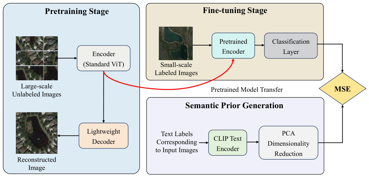
We propose a scene classification method based on a dynamic masking strategy and semantic enhancement. As illustrated in Algorithm 1 and Figure 1, the framework consists of two main stages—pre-training and fine-tuning:

Algorithm 1 Scene Classification via Dynamic Masking and Semantic Enhancement

Require: Unlabeled dataset $D_{\mathrm{train}}^u$; Labeled dataset $D_{\mathrm{train}}^l$; Text label set $C=\{c_1,\dots ,c_n\}$; Pretrained text encoder $E_{\mathrm{text}}$; Difficulty-prioritized masking ratios $P_{h0},P_{hf}$; EMA smoothing coefficient $k_s$; Total pre-training epochs N; Fine-tuning epochs $N_f$; Semantic label dimension d;

Ensure: Trained scene classification model

1: Stage 1: Pre-training

2: Sub-stage 1.1: Random Masking Initialization

3: for $\mathrm{epoch}=1$ to $N/2$ do

4:       For sample ${\mathit{x}}_i\in D_{\mathrm{train}}^u\cup D_{\mathrm{train}}^l$, randomly mask 75% of image patches and pre-train with MAE.

5:       Record the average reconstruction loss of each image patch in the later training period to compute the global reconstruction loss vector ${\mathit{L}}_0$.

6: end for

7: Sub-stage 1.2: Dynamic Masking

8: Initialize smoothed reconstruction loss ${\mathit{L}}_{\mathrm{ema}}={\mathit{L}}_0$

9: for $\mathrm{epoch}=N/2+1$ to N do

10:       Update difficulty-prioritized masking ratio $P_h$ and random masking ratio $P_r$.

11:       Based on ${\mathit{L}}_{\mathrm{ema}}^{t-1}$ from the previous epoch, prioritize masking the top $P_h$ proportion of image patches with the highest smoothed reconstruction loss, then randomly mask $P_r$ proportion of patches.

12:       Train the model (encoder $f_{\mathrm{E}}$ and decoder), and compute the current reconstruction loss ${\mathit{L}}_t$.

13:       Update ${\mathit{L}}_{\mathrm{ema}}$ via EMA: ${\mathit{L}}_{\mathrm{ema}}=k_s{\mathit{L}}_t+(1-k_s){\mathit{L}}_{\mathrm{ema}}^{t-1}$

14: end for

15: Stage 2: Semantic Enhancement Fine-Tuning

16: Extract and reduce the dimension of category semantic features to obtain semantic labels: ${\mathit{s}}_i=\mathrm{PCA}(E_{\mathrm{text}}\left(c_i\right),d)$

17: for $\mathrm{epoch}=1$ to $N_f$ do

18:       For sample $({\mathit{x}}_j,{\mathit{s}}_j)\in D_{\mathrm{train}}^l$, compute semantic loss: $\mathcal{L}=\mathrm{MSE}(f_{\mathrm{E}}\left({\mathit{x}}_j\right),{\mathit{s}}_j)$, and update parameters of $f_{\mathrm{E}}$.

19: end for

20: return Trained classification model $f_{\mathrm{E}}$

• Pre-training
  It is divided into two sub-stages: random masking initialization and dynamic masking. The initial stage uses random masking for pre-training and records per-patch reconstruction losses. In dynamic masking, the strategy is adaptively adjusted based on accumulated initial losses—prioritizing patches with higher reconstruction difficulty and gradually increasing their masking proportion to enhance feature learning. Per-patch losses are updated via exponential moving averaging (EMA), ensuring training stability while guiding the model to focus on complex semantic regions.
• Fine-tuning
  A pre-trained text encoder transforms categorical labels into high-dimensional semantic vectors, which are dimensionally reduced to obtain semantic embeddings. The model’s classification layer is redesigned to align with these embeddings. Incorporating semantic information alleviates the insufficient supervision of traditional MAE (which uses one-hot labels), enhancing classification capability.

3.1. Backbone

ViT adapts the Transformer architecture to computer vision (CV) tasks by partitioning images into patch sequences, mapping them to tokens, and feeding them into a Transformer encoder. Its self-attention mechanism enables global feature integration across patches.

We adopt ViT as the backbone for two key advantages:

• Superior global feature extraction, well-suited for remote sensing scene classification.
• Compatibility with MAE self-supervised pre-training, which fully utilizes unlabeled data to boost feature extraction.

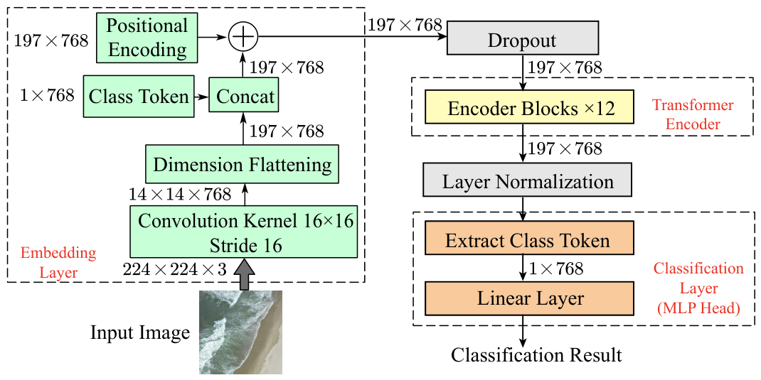
The backbone is ViT-B/16, a base ViT variant accepting $224\times 224\times 3$ RGB inputs (height × width × channels). The “16” denotes $16\times 16$ pixel patch size for segmentation—dividing the image into $14\times 14$ non-overlapping patches. Compared to other variants (e.g., ViT-L/16, ViT-H/14, ViT-S/16), it balances model scale and computational efficiency. ViT-B/16 comprises three components: embedding layer, Transformer encoder, and classification layer (Figure 2).

3.1.1. Embedding Layer

To convert 3D image inputs into a 2D matrix format compatible with the Transformer architecture, the layer performs three steps for an input image $\mathbf{X}\in {\mathbb{R}}^{H\times W\times C}$ (where H and W denote the height and width, respectively, and C represents channels): patch partitioning and linear projection, class token embedding, and positional encoding.

3.1.2. Transformer Encoder

The core component consists of stacked identical encoder blocks (Figure 3), each containing Multi-Head Self-Attention (MSA) and Multi-Layer Perceptron (MLP). Layer Normalization (LN) precedes each component to standardize features and accelerate convergence, while residual connections after MSA/MLP mitigate gradient vanishing. Consistent input/output dimensions enable seamless stacking for deep feature extraction.

3.1.3. Classification Layer

The MLP Head maps Transformer encoder outputs to classification results. ViT-B/16 outputs a $[197\times 768]$ tensor, from which the $[1\times 768]$ classification token is extracted—it aggregates holistic image information via self-attention, suitable for global scene classification.

3.2. Dynamic Masking Guided by Smooth Reconstruction Loss

ViT requires large-scale pre-training for optimal performance and is prone to overfitting on limited data. MAE enables effective self-supervised pre-training with unlabeled data, thereby alleviating overfitting.

Building on MAE, we propose a dynamic masking strategy guided by smooth reconstruction loss. By tracking and updating per-patch reconstruction losses, the strategy guides the model to focus masking on semantically challenging regions. The training process includes two sub-stages:

3.2.1. Random Masking Initialization

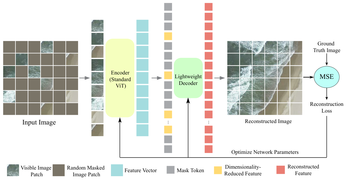
This stage (half of total pre-training epochs) uses a 75% masking ratio (consistent with traditional MAE) to enhance initial feature representation and provide initial reconstruction losses. For each batch image, patches are randomly masked; the encoder processes visible patches, and the decoder reconstructs masked regions to minimize reconstruction loss (Figure 3).

The MAE encoder is a standard ViT—directly used for downstream feature extraction without modification. It processes visible patch embeddings through a Transformer encoder (MSA + MLP) to extract contextual semantic features, which are fed into a lightweight Transformer decoder. The decoder reduces feature dimensions via linear projection, merges with learnable Mask Tokens, adds positional encodings, and reconstructs masked patch pixels through multiple layers.

The training objective minimizes masked region reconstruction loss. For each patch, Mean Squared Error (MSE) between predicted and target pixels is computed, with the final loss averaged over all masked regions:

$$L_{\mathrm{rec}}={\displaystyle \frac{{\sum }_{i=1}^L{m}_i·\mathrm{MSE}({\mathit{x}}_i^{\mathrm{tar}},{\mathit{x}}_i^{\mathrm{rec}})}{{\sum }_{i=1}^L{m}_i}}$$

(1)

where $m_i$ is the mask indicator ($m_i=1$ for masked patches), ${\mathit{x}}_i^{\mathrm{tar}}$ and ${\mathit{x}}_i^{\mathrm{rec}}$ are original and reconstructed pixel vectors, and L is total patches.

The decoder is discarded post-pre-training, so it is designed to be narrower and shallower (1/10 computational cost of the encoder). This asymmetric design reduces pre-training overhead while preserving encoder feature capability.

In the latter half of this stage (when training stabilizes), per-patch reconstruction losses are recorded and averaged across epochs to obtain the initial global loss vector ${\mathit{L}}_0$. For unmasked patches in an epoch, the epoch’s average patch loss is assigned to ensure complete statistics. ${\mathit{L}}_0$ provides the basis for subsequent dynamic masking.

3.2.2. Dynamic Masking

This stage combines difficulty-prioritized and random masking, guiding the model to focus on high-loss (semantically complex) patches. Per-patch losses are smoothly updated via EMA to inform masking strategy. The global loss vector ${\mathit{L}}_{\mathrm{ema}}$ (initialized as ${\mathit{L}}_0$) is updated at each epoch end:

$${\mathit{L}}_{\mathrm{ema}}=k_s{\mathit{L}}_t+(1-k_s){\mathit{L}}_{\mathrm{ema}}^{t-1}$$

(2)

where ${\mathit{L}}_t$ is the current epoch’s per-patch average loss vector, $k_s$ is the smoothing coefficient, and ${\mathit{L}}_{\mathrm{ema}}^{t-1}$ is the previous epoch’s smoothed loss. Larger ${\mathit{L}}_{\mathrm{ema}}$ values indicate harder-to-reconstruct patches, avoiding drastic masking fluctuations.

Each epoch’s masking strategy is generated using the previous ${\mathit{L}}_{\mathrm{ema}}$:

• Difficulty-prioritized masking: Sort patches by ${\mathit{L}}_{\mathrm{ema}}$ and mask the top $P_h$ proportion (applied to all images).
• Random masking: Randomly mask $P_r$ proportion of remaining patches to maintain 75% total masking (varies across images).

$P_h$ and $P_r$ are dynamically adjusted to reduce randomness and focus on challenging regions:

$$P_h=P_{h0}+\left({\displaystyle \frac{E_n}{E_t}}\right)\times (P_{hf}-P_{h0})$$

(3)

$$P_r=0.75-P_h$$

(4)

where $P_{h0}$ is the initial difficulty-based masking ratio, $E_n$ is the current epoch, and $E_t$ is the total dynamic masking epochs.

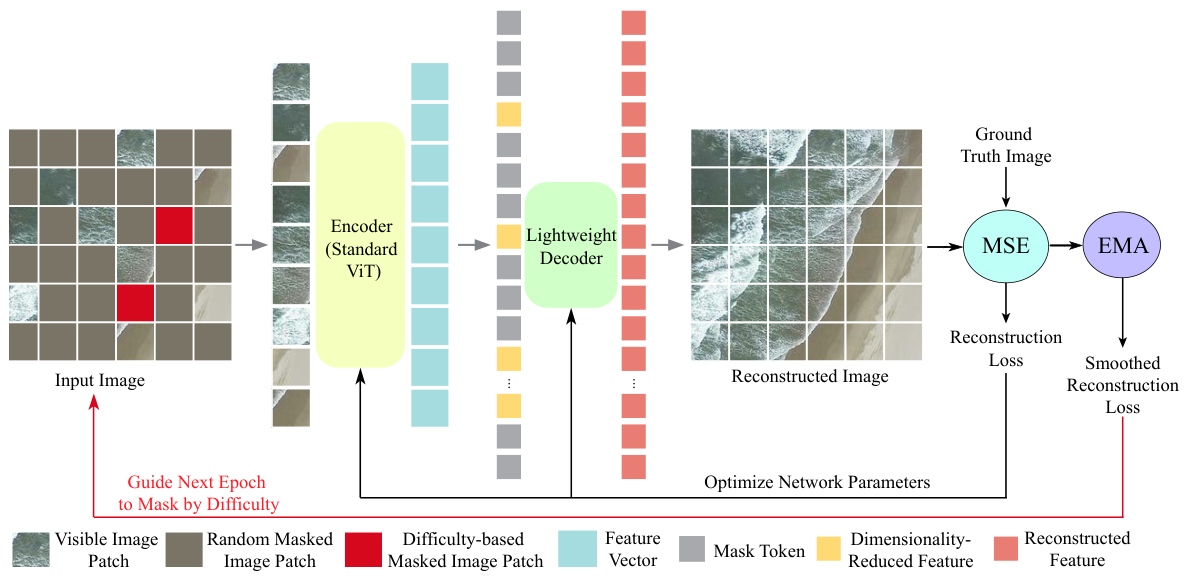
This design preserves early training randomness for exploration and gradually focuses on complex regions later. The workflow is shown in Figure 4.

3.2.3. Comparison with Existing Masking Strategies

To clarify the methodological distinction from existing masking strategies,

Table 1. Methodological comparison of representative masking strategies.

Method	Difficulty or Selection Criterion	Additional Learnable Parameters	Update Frequency	Adaptability
HOGMAE [32]	Handcrafted HOG-based structural prior	No	Per image; fixed criterion	Adapts to image structure, but not to the evolving reconstruction state
HPM [34]	Patch-wise reconstruction difficulty estimated by an auxiliary loss predictor	Yes	Jointly updated during pre-training	Adapts to model-estimated patch difficulty
SelectiveMAE [33]	Semantic-richness criterion for selective encoding and reconstruction	No auxiliary difficulty predictor	Per image; fixed criterion	Adapts to image content, but is not directly driven by reconstruction errors
SS-MAE [29]	Random spatial-patch and spectral-channel masking	Yes	Resampled for each input	Adapts to spatial–spectral characteristics, but not to reconstruction difficulty
Proposed Method	EMA-smoothed patch-wise reconstruction losses from the native MAE decoder	No auxiliary difficulty predictor	Updated at each epoch	Adapts to the evolving dataset-level reconstruction state while retaining random exploration

compares representative methods in terms of their difficulty or selection criterion, additional learnable parameters, update frequency, and adaptability. The proposed strategy is distinguished by jointly integrating native reconstruction-error feedback, EMA-based temporal smoothing, progressive difficulty scheduling, and random spatial exploration into a unified masking curriculum.

The proposed method is therefore not merely a parameter-reduced variant of difficulty-aware masking. Its main contribution lies in establishing a closed feedback loop between the model’s reconstruction state and the subsequent masking distribution. Native patch losses are temporally stabilized by EMA and converted into a progressively strengthened difficulty-prioritized component, while random masking preserves spatial diversity throughout pre-training. This complementary design provides an adaptive and stable curriculum without introducing an additional difficulty-prediction objective.

3.3. Cross-Modal Learning Based on Semantic Labels

To alleviate the limited semantic information provided by conventional one-hot labels, the downstream fine-tuning stage incorporates language-derived category semantics. Existing cross-modal remote sensing methods introduce semantic information through contrastive representation alignment or explicit label-relation modeling. In contrast, the proposed framework uses CLIP-encoded class names as fixed semantic prototypes and directly aligns visual outputs with these prototypes during downstream fine-tuning. This design preserves the independence of the MAE pre-training stage while introducing compact class-level semantic supervision without modifying the text encoder.

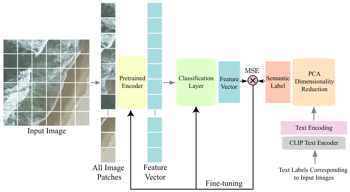
Specifically, the proposed cross-modal semantic enhancement framework comprises four sequential stages: text label encoding, semantic dimensionality reduction, classification layer redesign, and multimodal supervised learning (Figure 5).

3.3.1. Text Label Encoding

We use CLIP’s pre-trained text encoder (pre-trained on large-scale image-text pairs) to convert category labels into high-dimensional semantic vectors. For label $c_i$:

$${\mathit{t}}_i={\mathrm{CLIP}}_{\mathrm{Text}}\left(c_i\right)$$

(5)

where ${\mathrm{CLIP}}_{\mathrm{Text}}$ is the CLIP text encoder, and ${\mathit{t}}_i$ is the corresponding semantic vector. Similar categories (e.g., “lake” and “river”) have closer feature distances than dissimilar ones.

3.3.2. Semantic Dimensionality Reduction

High-dimensional text features (e.g., 512-dimensional CLIP outputs) may cause over-parameterization and overfitting. We apply PCA for dimensionality reduction:

$${\mathit{s}}_i=\mathrm{PCA}({\mathit{t}}_i,d)$$

(6)

where ${\mathit{s}}_i$ is the reduced-dimension semantic label, and d is a task-tunable hyperparameter. This preserves discriminative features and compacts the semantic space for efficient learning.

3.3.3. Classification Layer Redesign

Traditional classification layers use a fully connected layer (output dimension = number of classes) + Softmax. We redesign it to match the semantic label dimension:

$$\mathit{o}=f_{\theta }\left(\mathit{x}\right)$$

(7)

where $\mathit{x}$ is the encoder-extracted feature, $f_{\theta }$ is the redesigned layer, and $\mathit{o}$ is the d-dimensional output—enabling direct distance/similarity computation with semantic labels.

3.3.4. Multimodal Supervised Learning

A semantic distance-based loss guides alignment between model outputs and semantic labels. For sample ${\mathit{x}}_j$ with true category $y_j$ and semantic label ${\mathit{s}}_j$:

$$\mathcal{L}=\mathrm{MSE}(f_{\mathrm{E}}\left({\mathit{x}}_j\right),{\mathit{s}}_j)={\parallel f_{\mathrm{E}}\left({\mathit{x}}_j\right)-{\mathit{s}}_j\parallel }_2^2$$

(8)

where $f_{\mathrm{E}}(·)$ is the fine-tuned MAE encoder. MSE minimizes the squared Euclidean distance between predictions and semantic labels, leveraging inter-class semantic relationships for enhanced classification.

3.3.5. Inference

The predicted category is the one with the minimum Euclidean distance between the model output and semantic labels:

$$\underset{i\in \{1,\dots ,C\}}{\mathrm{argmin}}{\parallel f_{\mathrm{E}}\left({\mathit{x}}_j\right)-{\mathit{s}}_i\parallel }_2$$

(9)

where C is the total number of categories, and ${\mathit{s}}_i$ is the i-th category’s semantic label.

Furthermore, unlike traditional convolution-based autoencoders that are prone to the Gibbs phenomenon at mask boundaries, our approach leverages the patch-level processing mechanism and global self-attention computation of ViT. By performing reconstruction and semantic alignment predominantly in the feature space rather than imposing strong pixel-level continuous spatial constraints, this paradigm effectively mitigates boundary artifacts during mask reconstruction and cross-modal interaction.

3.3.6. Comparison with Existing Cross-Modal Learning Methods

Existing cross-modal remote sensing methods introduce semantic information through different technical routes. RS-CLIP [10] learns a shared vision–language embedding space through contrastive alignment, primarily supporting zero-shot and open-vocabulary recognition, while CMCL [35] strengthens cross-modal correspondences through contrastive supervision. CM-GM [36], in contrast, explicitly constructs semantic label graphs and combines Graph Convolutional Networks with bi-LSTM modules to model label dependencies for multi-label aerial image classification.

The proposed method targets sample-limited closed-set scene classification after MAE pre-training and follows a class-level semantic prototype regression paradigm. The frozen CLIP text encoder is used to generate fixed category prototypes, while the visual output is directly aligned with the ground-truth prototype through MSE during downstream fine-tuning. Compared with contrastive alignment and explicit label-graph modeling, the incremental contribution of the proposed scheme lies in decoupling self-supervised visual pre-training from compact semantic supervision. This formulation does not require paired image–text annotations, explicit label graphs, or recurrent relation-modeling modules, and its Euclidean regression objective is consistent with the nearest-prototype inference rule.

In summary, the proposed cross-modal module converts category names into fixed semantic prototypes and uses them as continuous supervisory targets during downstream fine-tuning. By decoupling self-supervised visual pre-training from class-level semantic alignment, the method introduces inter-class semantic relationships without requiring joint vision–language training, explicit label graphs, or recurrent relation-modeling modules. Moreover, the MSE-based prototype regression objective directly matches the Euclidean nearest-prototype inference rule, providing an effective and computationally efficient semantic supervision mechanism for sample-limited closed-set remote sensing scene classification.

4. Experiments

4.1. Datasets and Experimental Settings

The custom large-scale dataset $D_n$ was originally constructed and validated in [37]. To rigorously evaluate model robustness under complex, real-world constraints, $D_n$ was intentionally established to exhibit pronounced inter-class imbalance and intra-class variation. Specifically, the visual samples were integrated from multiple authoritative public remote sensing resources and data challenges, including NWPU-RESISC45, NWPU VHR-10, MAR20, RSOD, and RSCUP2019, supplemented by high-resolution imagery acquired from Google Earth. The spatial resolution of the images spans from 0.3 m to 2 m, capturing extensive environmental and sensor diversities across multi-temporal and multi-platform observations.

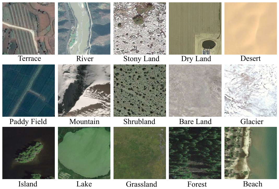
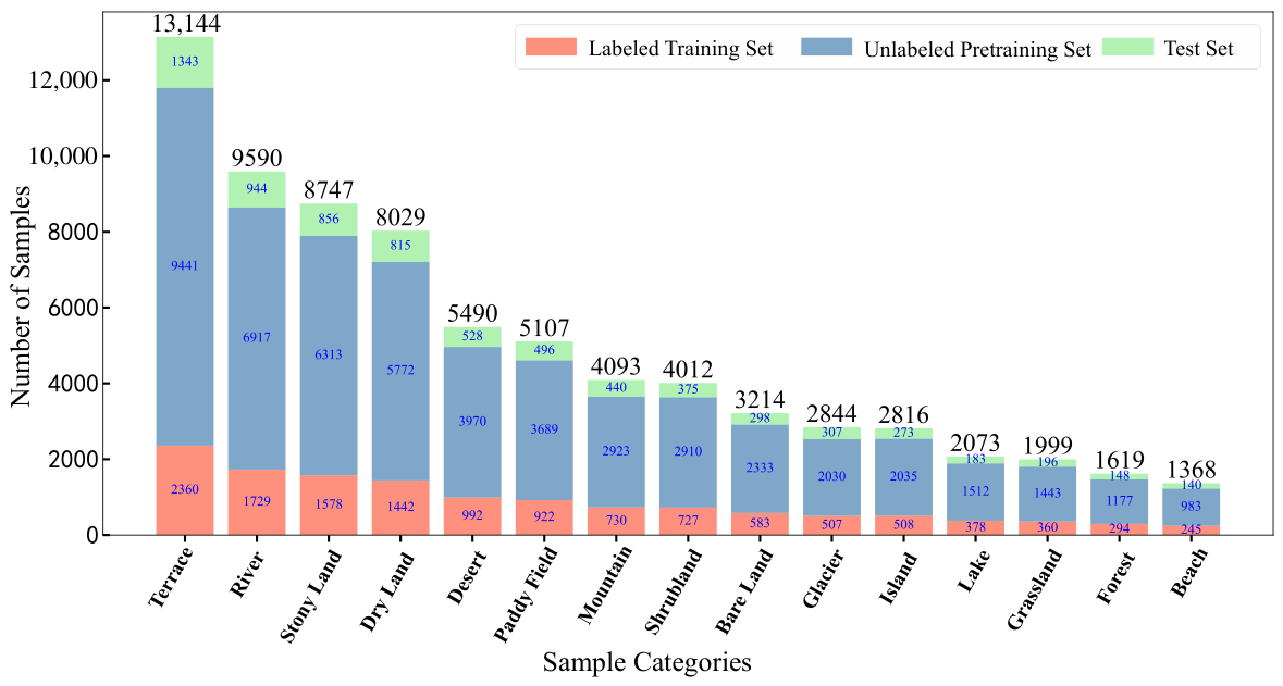
To guarantee experimental integrity and absolute reproducibility, a rigorous preprocessing and data cleaning workflow was strictly enforced based on the protocol established in [37]. First, an automated pixel-level hash check combined with manual inspection was executed across all source pools to eliminate redundant or overlapping patches, ensuring complete sample independence. Second, all collected images were uniformly normalized and resized to $256\times 256$ pixels. Third, the 9:1 partition between the training set ($D_{\mathrm{train}}$) and testing set ($D_{\mathrm{test}}$) was locked at the image level prior to any model training, ensuring absolutely zero data leakage or spatial cross-contamination. The detailed per-class sample numbers and training/testing splits for all 15 scene categories within $D_n$ are systematically summarized in

Table 2. Detailed sample distribution and partitioning specifications of the custom dataset $D_n$.

Category	Unlabeled ${\mathit{D}}_{\mathbf{train}}^{\mathit{u}}$	Labeled ${\mathit{D}}_{\mathbf{train}}^{\mathit{l}}$	Testing ${\mathit{D}}_{\mathbf{test}}$	Total
Terrace	9463	2366	1315	13,144
River	6905	1726	959	9590
Stony Land	6298	1574	875	8747
Dry Land	5781	1445	803	8029
Desert	3953	988	549	5490
Paddy Field	3677	919	511	5107
Mountain	2947	737	409	4093
Shrubland	2889	722	401	4012
Bare Land	2314	579	321	3214
Glacier	2048	512	284	2844
Island	2027	507	282	2816
Lake	1493	373	207	2073
Grassland	1439	360	200	1999
Forest	1166	291	162	1619
Beach	985	246	137	1368
Total	53,448	13,355	7342	74,145

. Representative samples and the class-wise sample distribution of dataset $D_n$ are shown in Figure 6 and Figure 7, respectively.

Additionally, an artificial remote sensing image dataset $D_a$ is constructed to evaluate the generalization of pre-trained models. Dataset $D_a$ contains 20 categories with a total of 16,612 RGB images, designed to simulate real-world scenarios with limited data availability. The image dimensions are uniformly set to $256\times 256$.

In addition to the self-constructed datasets, we further validate the effectiveness and generalization of our method on two widely used public remote sensing image scene classification benchmarks: the UCMerced (UCM) dataset [38] and the Aerial Image Dataset (AID) [39].

• UCM Dataset: The UCM dataset contains 2100 aerial images distributed across 21 land-use categories, with 100 images per class. The pixel resolution of each image is $256\times 256$. Given its relatively small scale, we randomly select 50% of the images in each category for training and the remaining 50% for testing.
• AID Dataset: The AID dataset is a large-scale aerial image dataset comprising 10,000 images spanning 30 diverse scene categories, representing more complex urban and rural environments. To rigorously evaluate the model’s performance under conditions of limited labeled data, we adopt a challenging split ratio, randomly assigning 20% of the images for training and the remaining 80% for testing.

During the pre-training phase, the AdamW optimizer was employed with a base learning rate of 0.0005 and a weight decay of 0.05. The learning rate was adjusted using a cosine annealing schedule. The pre-training process consisted of 200 epochs in total, with the first 100 epochs dedicated to random masking initialization and the subsequent 100 epochs for dynamic masking. We recorded the average reconstruction loss per image patch during the random masking initialization phase from epoch 75 to 100, and then used these values to initialize the per-patch reconstruction losses, aiming to guide the difficulty-aware masking in the first epoch of the dynamic masking stage. The total masking ratio was set to 75%, with a batch size of 128. In the dynamic masking stage, the EMA (Exponential Moving Average) smoothing coefficient $k_s$ was set to 0.5. To investigate the impact of difficulty-aware masking ratios, we tested four maximum difficulty masking ratios: 7.5%, 12.5%, 25%, and 50%.

During the fine-tuning stage, the AdamW optimizer was chosen as well, with a learning rate of 0.0001 and a weight decay of 0.05. The model was trained for 50 epochs with a batch size of 128. The pretrained CLIP text encoder was kept frozen when generating the class-level semantic prototypes. For the semantic label dimensionality reduction, we explored reducing 512-dimensional CLIP text features to various dimensions ranging from 2 to 15 to investigate the impact of semantic label dimension on model performance.

The hardware and software configurations for training and testing in the experiment are shown in

Table 3. The Software and Hardware Configurations in Experiments.

Name	Configuration
System	Windows 10
CPU Model	Intel Xeon Silver 4210
GPU Model	NVIDIA Quadro RTX 6000
Memory	256 GB
GPU Memory	24 GB
Anaconda Version	22.9.0
PyTorch Version	1.8.1
Python Version	3.7.16
CUDA Version	10.2.89

.

4.2. Results and Ablation Study

4.2.1. Results and Analysis

To comprehensively evaluate the performance of the proposed method, we compared it with multiple representative approaches.

Initially, a ViT-Base model was trained from scratch on $D_{\mathrm{train}}^l$, which served as the baseline performance using only labeled data. Secondly, a ViT model pre-trained via MAE on $D_{\mathrm{train}}$ and then fine-tuned on $D_{\mathrm{train}}^l$ was adopted as the foundational approach leveraging unlabeled data. Building upon this, we incorporated the state-of-the-art HPM method [34] for comparison. Additionally, we constructed a fully supervised model trained on complete labeled data as an ideal performance reference—i.e., the scenario where all samples in dataset $D_{\mathrm{train}}$ were labeled, corresponding to “Full Supervision” in

Table 4. Comparison of Classification Accuracy Across Different Methods on Remote Sensing Scene Classification Datasets. The MAE, HPM, and proposed-method results are reported as the mean ± standard deviation over five independent runs, whereas the remaining entries are reference results obtained under their corresponding settings.

Method	Pre-Training Strategy	Pre-Training Data	Accuracy (%, Mean ± STD)
ResNet-50	Train from scratch	—	86.5
ResNet-50	Full supervision	—	91.2
ViT-Base	Train from scratch	—	87.0
ViT-Base	MAE pre-training	$D_{\mathrm{train}}$	94.8 ± 0.23
ViT-Base	HPM	$D_{\mathrm{train}}$	94.9 ± 0.16
ViT-Base	Proposed method	$D_{\mathrm{train}}$	95.4 ± 0.07
ViT-Base	Full supervision	—	93.9

. The experimental results are shown in Table 4.

Under both from-scratch training and fully supervised training configurations, the ViT-Base achieved higher classification accuracy than ResNet-50. Specifically, in the from-scratch training setting with only dataset $D_{\mathrm{train}}^l$, ViT-Base outperformed ResNet-50 by 0.5% in accuracy. However, under the fully supervised configuration, the advantage of ViT-Base over ResNet-50 became more pronounced, with an improvement of 2.7%. These results demonstrate that the ViT-Base model based on Transformer architecture outperforms traditional CNNs in classification tasks, but its performance relies on large-scale labeled data through iterative training.

As shown in Table 4, the ViT-Base model trained from scratch performs the worst among the ViT-based configurations, achieving an accuracy of 87.0%. By leveraging unlabeled data through duration-matched MAE pre-training with random masking for 200 epochs, the classification accuracy increases substantially to 94.8%, confirming the effectiveness of self-supervised representation learning. The proposed method, which combines dynamic masking with semantic prototype supervision, further improves the accuracy to 95.4%, outperforming the 200-epoch MAE baseline and HPM by 0.6 and 0.5 percentage points, respectively. These gains demonstrate that the improvement cannot be attributed solely to the extended pre-training duration and further support the effectiveness of the proposed difficulty-guided masking and cross-modal semantic enhancement mechanisms. Compared with fully supervised ViT-Base training using all labeled samples (93.9%), the proposed method also achieves a 1.5-percentage-point improvement, indicating that appropriately designed self-supervised pre-training and semantic supervision can effectively exploit unlabeled data and language-derived category information.

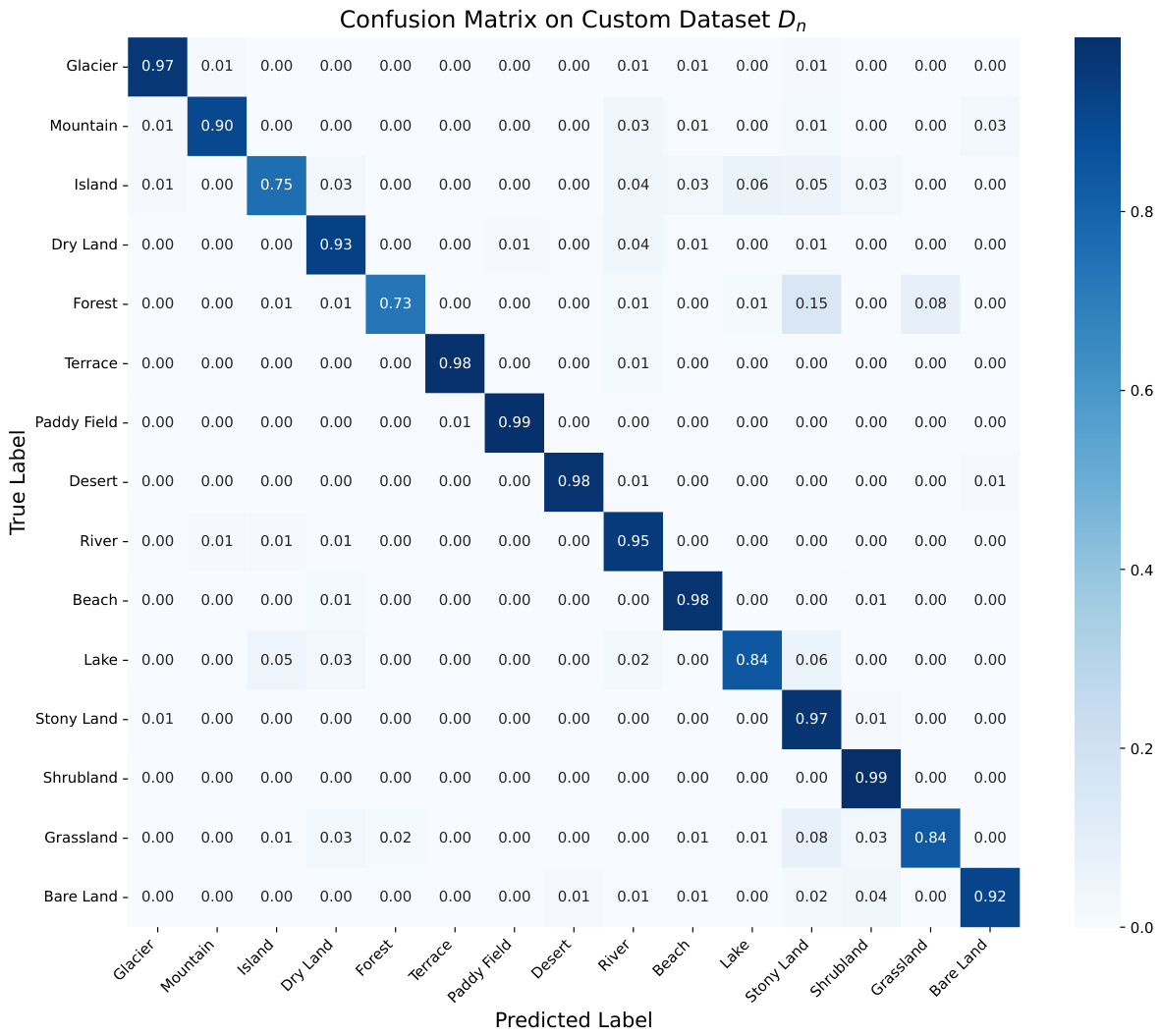
To gain deeper insights into the classification performance, we plotted the normalized confusion matrix on the test set of dataset $D_n$ (Figure 8). The model demonstrates robust discriminative capabilities, with most categories exceeding 93% accuracy. Notably, it successfully disentangles visually homogeneous categories like “River” (95% accuracy, with only 2% misclassified as “Lake”), effectively demonstrating the superiority of the cross-modal semantic enhancement.

Nevertheless, minor misclassifications occur in complex scenarios, primarily for “Forest” (73% accuracy, mainly confused with “Stony Land”) and “Island” (75% accuracy, confused with “Lake”). These errors inherently stem from the physical co-occurrence and ambiguous boundaries of geographical features in real-world aerial imagery (e.g., forests growing on stony terrains, or islands encompassed by lakes). Despite these challenging mixed-pixel representations, the overall confusion rates are tightly constrained, further validating the robustness of our framework.

In addition, to evaluate the computational efficiency of the proposed method, we assess its computational complexity, parameter count, and wall-clock runtime, as summarized in

Table 5. Comparison of Computational Efficiency Across Different Methods.

Method	Parameters (M)	Batch Size	Time (s/epoch)	FLOPs (G)
MAE	111.91	128	271	9.43
HPM	137.52	100	783	23.61
Proposed Method	111.91	128	273	9.48

.

During pre-training, the proposed dynamic masking strategy introduced minimal additional computational overhead compared to the original MAE method, primarily for updating and maintaining the reconstruction loss vectors of image patches. The computational time (273 s/epoch) and floating-point operations (9.48 GFLOPs) of the proposed method increased by less than 1% compared to MAE (271 s/epoch, 9.43 GFLOPs). However, the HPM method introduced an additional loss prediction layer, which increased the model parameters by 22.9%. Due to memory constraints on the RTX6000 GPU, the training batch size had to be reduced from 128 to 100, resulting in a training time increase of approximately 189% (from 271 s to 783 s). This demonstrates that the proposed dynamic masking strategy can effectively optimize pre-training performance while significantly outperforming the HPM method in terms of computational efficiency.

During fine-tuning, the proposed method introduces two major modifications to the ViT model:

• Adjust the output dimension of the classification layer from the number of classes to the semantic feature dimension.
• Change the loss function from cross-entropy loss to MSE (Mean Squared Error).

As a result of these modifications during fine-tuning, since the adopted semantic feature dimension (e.g., 14) is strictly less than the total number of classes (15), the overall parameter count of the proposed classification head is marginally reduced compared to the baseline MAE. Additionally, regarding the preprocessing of semantic labels—including CLIP text encoding and PCA dimensionality reduction—this involves minimal computational overhead because it only requires processing the encoding and dimensionality reduction of a number of textual tokens equal to the number of classes (15 in $D_n$). This computation is minimal and performed offline, thus not affecting the training or inference efficiency of the model. Therefore, compared to the baseline model MAE, the proposed method introduces negligible additional computational overhead during fine-tuning and inference. Considering the performance gains it achieves, this marginal efficiency trade-off is acceptable and is of great significance in practical applications.

To validate the generalization of the proposed method, the model pre-trained on the natural-scene remote sensing image dataset ($D_n$) was applied to classification tasks on the artificial-scene remote sensing image dataset ($D_a$). As shown in

Table 6. Generalization Performance Comparison of Different Pre-training Strategies.

Network Model	Pre-Training Strategy	Label Type	Accuracy (%)
ViT+Softmax	—	One-hot	68.4
ViT+Tanh	—	Semantic	69.1
ViT+Softmax	MAE	One-hot	81.5
ViT+Tanh	MAE + Dynamic Masking	Semantic	83.5

, without additional pre-training, the model using semantic labels (69.1%) achieved a marginal performance improvement over traditional one-hot labels (68.4%), demonstrating the fundamental effectiveness of the semantic labeling scheme proposed in this paper. Importantly, when incorporating the pre-trained weights from MAE, the classification performance showed significant improvement: the model with standard MAE pre-training achieved an accuracy of 81.5%, while the complete solution combining the dynamic masking strategy and semantic label supervision further enhanced performance to 83.5%. The experimental results demonstrate that when the target domain data is limited, the proposed pre-training strategy significantly impacts model performance. Furthermore, the proposed method maintains its effectiveness in cross-scene scenarios, achieving higher classification accuracy compared to baseline approaches.

To evaluate the cross-dataset generalization capability of the proposed method, we first conducted unsupervised pre-training on the large-scale NWPU dataset [40] without using any label information. The pretrained models were then transferred to the UCM and AID public benchmarks and compared with representative baselines, as reported in

Table 7. Classification accuracy (%) comparison (Mean ± STD) across different methods on public benchmarks using identical splits.

Method	UCM (50%)	AID (20%)
ResNet-50 [41]	$98.25\pm 0.66$	$92.57\pm 0.17$
CNN-CapsNet [42]	$97.59\pm 0.16$	$93.79\pm 0.13$
ViT-B [8]	$98.58\pm 0.15$	$94.90\pm 0.29$
Swin-T [43]	$98.94\pm 0.10$	$94.56\pm 0.14$
DaViT [44]	$98.90\pm 0.13$	$95.48\pm 0.13$
ToMe [45]	$98.54\pm 0.10$	$95.19\pm 0.09$
DEMS-ViT [46]	$98.48\pm 0.18$	$95.22\pm 0.17$
Proposed Method	98.96 ± 0.05	95.73 ± 0.08

. To assess data efficiency under limited-label settings, the models were fine-tuned using 50% of the UCM images and 20% of the AID images, following the evaluation protocols described above.

To eliminate the contingency of an individual random split and ensure a mathematically rigorous evaluation, all experiments conducted on the public UCM and AID benchmarks were executed independently for five runs using distinct random initialization seeds. For all compared baseline methods and our proposed framework, we report the mean Overall Accuracy (OA) coupled with the standard deviation (± STD). Furthermore, to guarantee absolute fairness, identical image-level random partitions were enforced simultaneously across all models during each respective evaluation trial.

Under this setting, our method achieves 98.96% on UCM and 95.73% on AID. On the AID dataset, despite using less training data, the proposed method outperforms ResNet-50 by 3.16% and exceeds DaViT and ToMe by 0.25% and 0.54%, respectively. These results indicate that the combination of dynamic masking and cross-modal semantic enhancement facilitates efficient feature learning across different remote sensing scenes.

4.2.2. Ablation Study

Dynamic Masking Strategy

To validate the effectiveness of the proposed dynamic masking strategy guided by smooth reconstruction loss, we conducted two complementary sets of experiments. First, we compared the proposed strategy with vanilla MAE, HPM, SelectiveMAE, and SS-MAE. To separate the contribution of the masking policy from that of the pre-training duration, we additionally included a duration-matched MAE baseline trained for 200 epochs using random masking throughout the entire pre-training process. HPM, SelectiveMAE, SS-MAE, and the proposed method were also trained for 200 epochs under the same backbone, dataset, optimizer, learning-rate schedule, total masking ratio, and downstream evaluation protocol. Second, we investigated the effect of the ratio between difficulty-prioritized masking and random masking while maintaining a total masking ratio of 75%.

Two evaluation protocols were employed: linear probing and full fine-tuning. For linear probing, all Transformer encoder layers of the pre-trained model were frozen, and only the newly added linear classification layer was optimized, providing a direct assessment of the learned feature representations. For full fine-tuning, all network parameters were updated to evaluate downstream classification performance. The results are presented in

Table 8. Performance comparison of different masking strategies and pre-training schedules.

Method	Pre-Training Epochs	Masking Schedule	Linear Probe (%)	Fine-Tuning (%)
MAE (short schedule)	100	Random × 100	88.3	94.4
MAE (duration-matched)	200	Random × 200	88.5	94.8
HPM	200	Method-specific masking	88.2	94.9
SelectiveMAE	200	Method-specific masking	88.4	95.1
SS-MAE	200	Method-specific masking	88.5	95.2
MAE + Dynamic Masking (Ours)	200	Random × 100 + Dynamic × 100	88.7	95.4

.

As shown in Table 8, extending vanilla MAE pre-training from 100 to 200 epochs improves the linear-probing accuracy from 88.3% to 88.5% and the fine-tuning accuracy from 94.4% to 94.8%, indicating that a longer pre-training duration contributes to representation learning. More importantly, under the strictly duration-matched 200-epoch setting, the proposed dynamic masking strategy further increases the linear-probing and fine-tuning accuracies to 88.7% and 95.4%, respectively. Compared with the full-random MAE baseline trained for the same 200 epochs, our method achieves additional gains of 0.2 and 0.6 percentage points. Because the two configurations share the same backbone, training data, optimization settings, total masking ratio, and pre-training duration, this controlled comparison provides direct evidence that the improvement is attributable to the proposed difficulty-guided masking curriculum rather than merely to the additional training epochs.

The proposed method also consistently achieves the best performance among all evaluated 200-epoch masking strategies under both evaluation protocols. In full fine-tuning, it surpasses HPM, SelectiveMAE, and SS-MAE by 0.5, 0.3, and 0.2 percentage points, respectively, while maintaining corresponding advantages in linear probing. These consistent improvements demonstrate that the proposed strategy learns more transferable and discriminative representations by jointly exploiting reconstruction-difficulty-guided priority masking and random spatial exploration. The difficulty-guided component encourages the encoder to repeatedly address challenging patch positions, whereas the random component maintains sufficient spatial diversity and prevents the masking process from collapsing into a fixed pattern. Their complementary interaction establishes a more effective pre-training curriculum and leads to superior downstream classification performance.

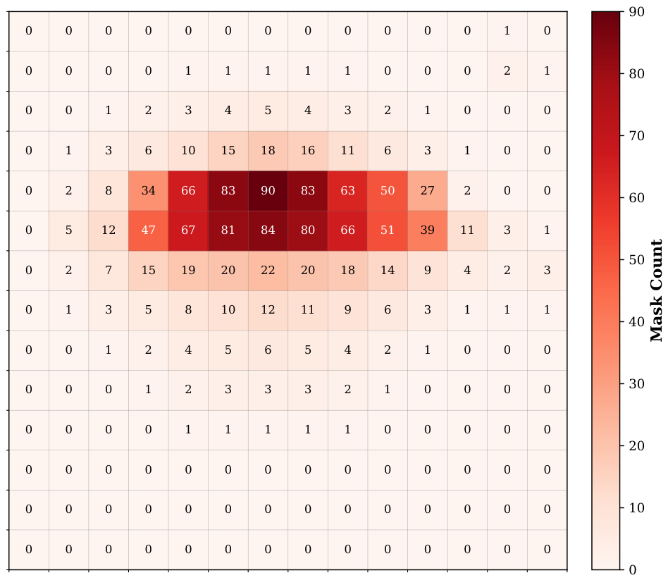
To characterize the spatial behavior of the difficulty-prioritized component, Figure 9 reports the cumulative selection frequency of each patch position throughout the dynamic masking stage. The resulting distribution is clearly non-uniform: patch positions near the central region are selected more frequently, with the maximum count reaching 90, whereas the frequencies gradually decrease toward the image boundaries. This pattern is consistent with the spatial composition of many standardized remote sensing images, in which prominent geographical structures are often located near the central field of view. Meanwhile, several peripheral positions retain sparse but non-zero selection counts, showing that the priority allocation is not restricted to a rigid central window. Overall, the heatmap provides a dataset-level statistical view of how the proposed curriculum concentrates part of the masking budget on frequently difficult spatial regions, while the accompanying random masking component preserves broader spatial exploration.

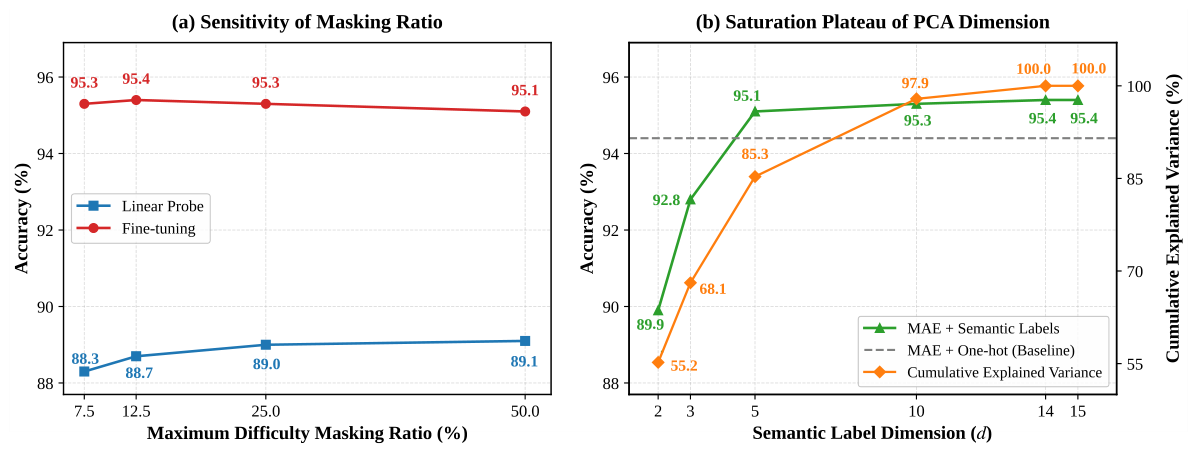
The numerical variations are summarized in

Table 9. Sensitivity analysis of the maximum difficulty-prioritized masking ratio.

Max Ratio (%)	Linear Probe (%)	Fine-Tuning (%)
7.5	88.3	95.3
12.5	88.7	95.4
25.0	89.0	95.3
50.0	89.1	95.1

, and the macro trends are plotted in Figure 10a. As illustrated in Figure 10a, under the frozen linear probing configuration, the network’s representation capacity scales monotonically with higher difficulty-based masking proportions, indicating that focusing on complex reconstruction patches enriches spatial feature abstractions. Under the downstream fine-tuning paradigm, however, the overall accuracy exhibits a characteristic parabolic trajectory, peaking at 95.4% exactly at a 12.5% ratio before decaying. This optimization cliff reveals that while too low a ratio under-challenges the Vision Transformer, an excessive difficulty bias over-suppresses random patch exploration, causing the network to overfit to local edge anomalies and impairing generalized feature discovery.

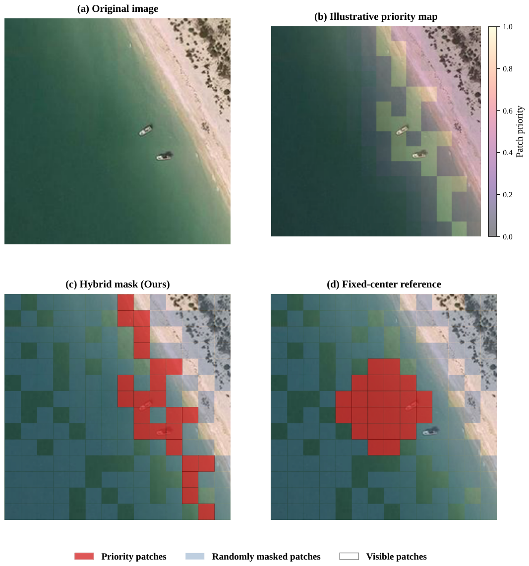
To provide an intuitive view of how the spatial placement of priority patches influences the masking pattern, Figure 11 presents a controlled illustrative comparison on an asymmetric beach scene. The selected image contains a slanted shoreline and two small vessels located away from the geometric center. As shown in Figure 11b, the illustrative patch-priority map assigns higher priority to the shoreline and local object regions, while the comparatively homogeneous water area receives lower priority. Figure 11c converts this structure-oriented priority arrangement into a hybrid masking layout by combining the priority patches with randomly masked patches.

For comparison, Figure 11d replaces the structure-oriented priority component with a fixed-center arrangement, while retaining the same total masking ratio and the same numbers of priority, random, and visible patches. Overall, this controlled comparison highlights the spatial flexibility of the proposed hybrid masking principle, which combines broad random exploration with targeted emphasis on structurally informative regions beyond the geometric center.

Cross-Modal Learning with Semantic Labels

To comprehensively evaluate the proposed cross-modal semantic enhancement module, we investigate two complementary design factors. First, we compare different cross-modal supervision objectives, including Cosine Similarity, RS-CLIP-style contrastive alignment based on InfoNCE, and the proposed MSE-based semantic prototype regression. Second, we analyze the influence of the PCA-reduced semantic label dimension on downstream classification performance. The comparison of supervision objectives is presented in

Table 10. Controlled comparison of cross-modal supervision objectives in terms of classification accuracy and training efficiency.

Cross-Modal Supervision	Time (s/epoch)	Linear Probe (%)	Fine-Tuning (%)
Cosine Similarity	285	88.1	94.8
RS-CLIP-style Contrastive Alignment (InfoNCE)	512	88.4	95.1
MSE-Based Semantic Prototype Regression (Ours)	273	88.7	95.4

, while the semantic-dimension analysis is summarized in

Table 11. Relationship between PCA information retention and downstream classification accuracy.

Semantic Dimension (d)	Cumulative Explained Variance (%)	Fine-Tuning Accuracy (%)
2	55.2	89.9
3	68.1	92.8
5	85.3	95.1
10	97.9	95.3
14	100.0	95.4
15	100.0	95.4

.

For the objective-level comparison, all configurations use the same MAE-pretrained visual encoder, CLIP-derived and PCA-reduced semantic prototypes, training samples, optimizer, batch size, learning-rate schedule, and fine-tuning epochs. Only the cross-modal supervision objective is changed. In the RS-CLIP-style InfoNCE configuration, each image representation and its ground-truth class prototype form a positive pair, while the remaining class prototypes serve as negatives. This controlled setting isolates the influence of the supervision objective from other architectural and training differences.

As shown in Table 10, the proposed MSE-based semantic prototype regression achieves the best performance under both evaluation protocols, reaching 88.7% in linear probing and 95.4% after full fine-tuning. Under otherwise identical experimental settings, the RS-CLIP-style InfoNCE objective achieves 88.4% and 95.1%, respectively. The proposed MSE formulation therefore provides consistent improvements of 0.3 percentage points in both evaluation settings. Cosine Similarity obtains accuracies of 88.1% and 94.8%, further indicating that direct semantic-coordinate regression is more effective than angular alignment alone for the task considered in this study.

The proposed MSE formulation also demonstrates a clear computational advantage. The RS-CLIP-style InfoNCE configuration constructs and normalizes image–prototype similarity scores involving positive and negative pairs, resulting in a training time of 512 s per epoch. In contrast, MSE directly regresses each visual representation toward its target semantic prototype and requires only 273 s per epoch, corresponding to a 46.7% reduction in per-epoch training time relative to the contrastive configuration. MSE also remains slightly more efficient than Cosine Similarity, which requires 285 s per epoch.

These results demonstrate that the proposed MSE objective is particularly well suited to the closed-set semantic-prototype learning setting adopted in this study. Its Euclidean distance-minimization objective is directly consistent with the nearest-prototype decision rule used during inference, while avoiding explicit negative-pair construction and temperature-dependent similarity ranking. Consequently, the proposed scheme provides a more direct, accurate, and computationally efficient cross-modal supervision mechanism for sample-limited remote sensing scene classification with fixed semantic prototypes.

After establishing the effectiveness of the cross-modal supervision objective, we further evaluate the contribution of semantic-label supervision and investigate the influence of the PCA-reduced semantic dimension on classification performance. The corresponding results are summarized in Table 11.

Table 11 and Figure 10b jointly quantify the relationship between PCA information retention and downstream classification performance. When the semantic dimension increases from $d=2$ to $d=5$, the cumulative explained variance rises from 55.2% to 85.3%, accompanied by a substantial improvement in fine-tuning accuracy from 89.9% to 95.1%. This trend indicates that excessively low-dimensional representations discard semantic variations that are important for distinguishing related remote sensing categories. Notably, the accuracy at $d=5$ already exceeds the conventional one-hot baseline of 94.4%, demonstrating the effectiveness of compact language-derived semantic supervision.

As the semantic dimension is further increased, the cumulative explained variance reaches 97.9% at $d=10$ and 100.0% at $d=14$, while the corresponding classification accuracy gradually improves to 95.3% and 95.4%, respectively. Increasing the dimension from 14 to 15 introduces no additional explained variance and produces no further accuracy gain, indicating that the semantic representation has reached a stable saturation point. Therefore, $d=14$ is selected as the final configuration because it preserves the complete effective semantic information captured by PCA, achieves the highest classification accuracy, and maintains a compact output space for efficient semantic prototype learning.

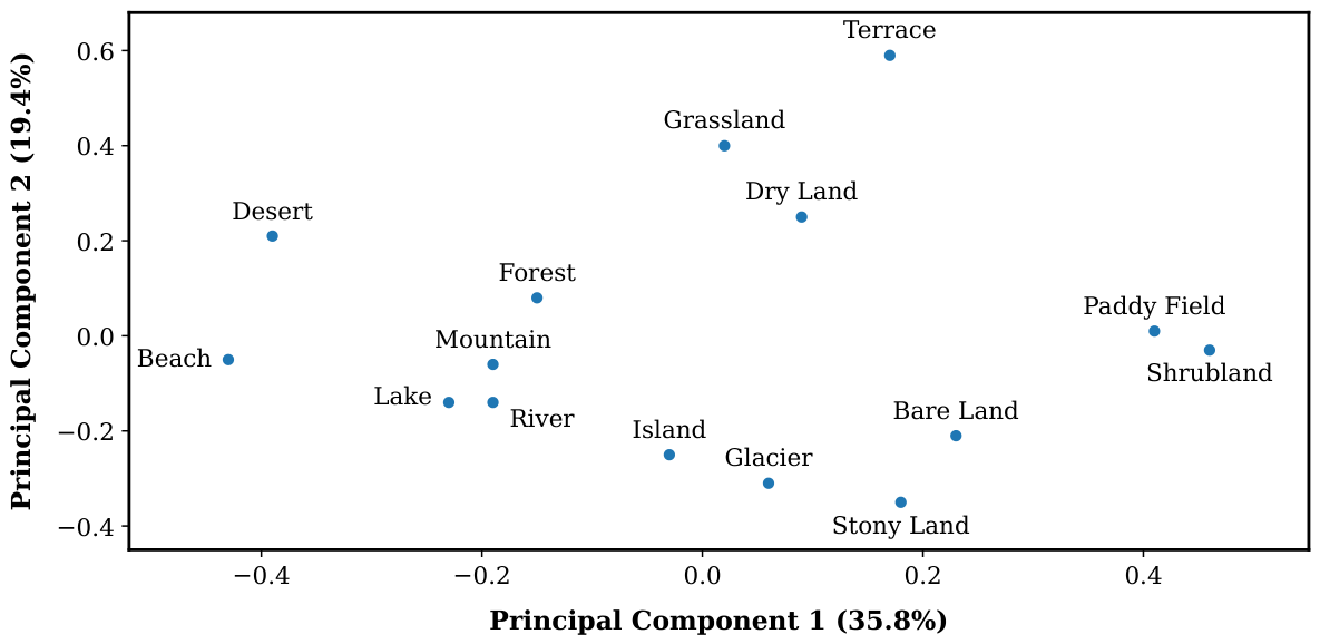
To visualize the relative organization of the class-level semantic prototypes, Figure 12 projects the CLIP-derived text features onto the first two principal components. PC1 and PC2 explain 35.8% and 19.4% of the total semantic variance, respectively, corresponding to a cumulative value of 55.2%. This two-dimensional projection is used only for visualization, rather than as the final semantic supervision space. The distribution shows that semantically related categories, such as “river” and “lake”, occupy nearby regions, whereas more distinct categories, such as “river” and “desert”, are more widely separated. This qualitative structure supports the use of language-derived prototypes as richer supervisory targets than independent one-hot labels.

5. Conclusions

For remote sensing scene classification tasks, we propose a novel method based on dynamic masking and cross-modal semantic learning with semantic information enhancement, which addresses the challenge of how to fully utilize large-scale unlabeled data to enhance the classification performance of deep learning approaches. Through innovations in both pre-training and fine-tuning stages, our approach enhances feature learning from unlabeled image data while fully leveraging the semantic information embedded in text labels, thereby achieving significant improvements over traditional MAE methods and enhancing model performance in remote sensing image scene classification tasks. The experimental results demonstrate that the proposed method not only maintains pre-training efficiency but also exhibits strong classification performance and excellent generalization. Consequently, these characteristics underscore the practical value of the proposed method in mitigating sample scarcity across large-scale, unlabeled remote sensing scenarios under specialized conditions.

References

1. Cheng, G.; Xie, X.; Han, J.; Guo, L.; Xia, G.S. Remote Sensing Image Scene Classification Meets Deep Learning: Challenges, Methods, Benchmarks, and Opportunities. IEEE J. Sel. Top. Appl. Earth Obs. Remote Sens. 2020, 13, 3735–3756. [Google Scholar] [CrossRef] [Scilit]
2. Wang, Q.; Huang, W.; Xiong, Z.; Li, X. Looking Closer at the Scene: Multiscale Representation Learning for Remote Sensing Image Scene Classification. IEEE Trans. Neural Netw. Learn. Syst. 2020, 33, 1414–1428. [Google Scholar]
3. Yang, Y.; Jiao, L.; Liu, X.; Liu, F.; Yang, S.; Li, L.; Chen, P.; Li, X.; Huang, Z. Dual wavelet attention networks for image classification. IEEE Trans. Circuits Syst. Video Technol. 2023, 33, 1899–1910. [Google Scholar] [CrossRef] [Scilit]
4. Hong, D.; Gao, L.; Yokoya, N.; Yao, J.; Chanussot, J.; Du, Q.; Zhang, B. More diverse means better: Multimodal deep learning meets remote sensing imagery classification. IEEE Trans. Geosci. Remote Sens. 2020, 59, 4340–4354. [Google Scholar]
5. Bi, M.; Wang, M.; Li, Z.; Hong, D. Vision transformer with contrastive learning for remote sensing image scene classification. IEEE J. Sel. Top. Appl. Earth Obs. Remote Sens. 2022, 16, 738–749. [Google Scholar]
6. Deng, P.; Xu, K.; Huang, H. When CNNs Meet Vision Transformer: A Joint Framework for Remote Sensing Scene Classification. IEEE Geosci. Remote Sens. Lett. 2021, 19, 8020305. [Google Scholar]
7. Lv, P.; Wu, W.; Zhong, Y.; Du, F.; Zhang, L. Scvit: A Spatialchannel Feature Preserving Vision Transformer for Remote Sensing Image Scene Classification. IEEE Trans. Geosci. Remote Sens. 2022, 60, 4409512. [Google Scholar] [CrossRef] [Scilit]
8. Dosovitskiy, A.; Beyer, L.; Kolesnikov, A.; Weissenborn, D.; Zhai, X.; Unterthiner, T.; Dehghani, M.; Minderer, M.; Heigold, G.; Gelly, S.; et al. An image is worth 16x16 words: Transformers for image recognition at scale. In Proceedings of the International Conference on Learning Representations, Virtual, 3–7 May 2021. [Google Scholar]
9. Aleissaee, A.A.; Kumar, A.; Anwer, R.M.; Khan, S.; Cholakkal, H.; Xia, G.S.; Khan, F.S. Transformers in remote sensing: A survey. Remote Sens. 2023, 15, 1860. [Google Scholar] [CrossRef] [Scilit]
10. Li, X.; Wen, C.; Hu, Y.; Zhou, N. RS-CLIP: Zero shot remote sensing scene classification via contrastive vision-language supervision. Int. J. Appl. Earth Obs. Geoinf. 2023, 124, 103497. [Google Scholar] [CrossRef] [Scilit]
11. Alajaji, D.; Alhichri, H.S.; Ammour, N.; Alajlan, N. Few-Shot Learning For Remote Sensing Scene Classification. In Proceedings of the 2020 Mediterranean and Middle-East Geoscience and Remote Sensing Symposium (M2GARSS), Tunis, Tunisia, 9–11 March 2020; pp. 81–84. [Google Scholar]
12. Wang, H.; Ye, Z.; Wang, Y.; Liu, X.; Zhang, X.; Zhao, Y.; Li, S.; Liu, Z.; Zhang, X. Improving the crop classification performance by unlabeled remote sensing data. Expert Syst. Appl. 2024, 236, 121283. [Google Scholar] [CrossRef] [Scilit]
13. Bai, K.; Mu, X.; Chen, X.; Zhu, Y.; You, X. Unsupervised Remote Sensing Image Scene Classification Based on Semi-Supervised Learning. Acta Geod. Cartogr. Sin. 2022, 51, 691–702. [Google Scholar]
14. Wang, Y.; Albrecht, C.M.; Braham, N.A.A.; Mou, L.; Zhu, X.X. Self-supervised learning in remote sensing: A review. IEEE Geosci. Remote Sens. Mag. 2022, 10, 213–247. [Google Scholar] [CrossRef] [Scilit]
15. Li, Y.; Zhu, Z.; Yu, J.G.; Zhang, Y. Learning deep cross-modal embedding networks for zero-shot remote sensing image scene classification. IEEE Trans. Geosci. Remote Sens. 2021, 59, 10590–10603. [Google Scholar] [CrossRef] [Scilit]
16. Jung, H.; Choi, H.S.; Kang, M. Boundary enhancement semantic segmentation for building extraction from remote sensed image. IEEE Trans. Geosci. Remote Sens. 2022, 60, 5215512. [Google Scholar] [CrossRef] [Scilit]
17. He, X.; Zhou, Y.; Zhao, J.; Zhang, D.; Yao, R.; Xue, Y. Swin transformer embedding UNet for remote sensing image semantic segmentation. IEEE Trans. Geosci. Remote Sens. 2022, 60, 4408715. [Google Scholar] [CrossRef] [Scilit]
18. Li, J.; Zheng, K.; Li, Z.; Gao, L.; Jia, X. X-Shaped Interactive Autoencoders With Cross-Modality Mutual Learning for Unsupervised Hyperspectral Image Super-Resolution. IEEE Trans. Geosci. Remote Sens. 2023, 61, 5518317. [Google Scholar] [CrossRef] [Scilit]
19. Xu, H.; Ran, G.; Cai, Y.; Wang, Y.; Bi, S. LESFuse: A lightweight dual-domain collaborative framework for high-fidelity visible-infrared image fusion. Appl. Soft Comput. 2026, 193, 114805. [Google Scholar] [CrossRef] [Scilit]
20. Grill, J.B.; Strub, F.; Altché, F.; Tallec, C.; Richemond, P.; Buchatskaya, E.; Doersch, C.; Avila Pires, B.; Guo, Z.; Gheshlaghi Azar, M.; et al. Bootstrap Your Own Latent: A New Approach to Self-Supervised Learning. Adv. Neural Inf. Process. Syst. 2020, 33, 21271–21284. [Google Scholar]
21. Chen, T.; Kornblith, S.; Norouzi, M.; Hinton, G.E. A Simple Framework for Contrastive Learning of Visual Representations. Int. Conf. Mach. Learn. 2020, 119, 1597–1607. [Google Scholar]
22. Guo, D.; Xia, Y.; Luo, X.; Feng, J. Remote Sensing Image Scene Classification Based on Supervised Contrastive Learning. Acta Photon. Sin. 2021, 50, 87–98. [Google Scholar]
23. Yu, X.; Wu, X.; Luo, C.; Ren, P. Deep learning in remote sensing scene classification: A data augmentation enhanced convolutional neural network framework. GISci. Remote Sens. 2017, 54, 741–758. [Google Scholar] [CrossRef] [Scilit]
24. Zhao, H.; Zhang, J.; Zhu, J.; Li, H. Image Classification Framework Based on Contrastive Self-Supervised Learning. J. Jilin Univ. (Eng. Technol. Ed.) 2022, 52, 1850–1856. [Google Scholar]
25. Zhang, C.; Chen, J.; Li, Q.; Deng, B.; Wang, J.; Chen, C. Deep Contrastive Learning: A Survey. Acta Autom. Sin. 2023, 49, 15–39. [Google Scholar]
26. Hu, H.; Wang, X.; Zhang, Y.; Chen, Q.; Guan, Q. A Comprehensive Survey on Contrastive Learning. Neurocomputing 2024, 578, 128645. [Google Scholar] [CrossRef] [Scilit]
27. Devlin, J.; Chang, M.W.; Lee, K.; Toutanova, K. BERT: Pre-training of Deep Bidirectional Transformers for Language Understanding. In Proceedings of the 2019 Conference of the North American Chapter of the Association for Computational Linguistics: Human Language Technologies; Association for Computational Linguistics: Minneapolis, MN, USA, 2–7 June 2019; pp. 4171–4186. [Google Scholar]
28. He, K.; Chen, X.; Xie, S.; Li, Y.; Dollár, P.; Girshick, R. Masked autoencoders are scalable vision learners. In Proceedings of the IEEE/CVF Conference on Computer Vision and Pattern Recognition (CVPR), New Orleans, LA, USA, 19–24 June 2022; pp. 16000–16009. [Google Scholar]
29. Lin, J.; Gao, F.; Shi, X.; Dong, J.; Du, Q. SS-MAE: Spatial–spectral masked autoencoder for multisource remote sensing image classification. IEEE Trans. Geosci. Remote Sens. 2023, 61, 5531614. [Google Scholar] [CrossRef] [Scilit]
30. Sun, L.; Lian, Z.; Liu, B.; Tao, J. MAE-DFER: Efficient masked autoencoder for self-supervised dynamic facial expression recognition. In Proceedings of the 31st ACM International Conference on Multimedia, Ottawa, ON, Canada, 29 October–3 November 2023; pp. 6110–6121. [Google Scholar]
31. Li, Z.; Shao, Y.; Zhang, F.; Zhang, J.; Wang, Y.; Sang, N. Difficulty-aware dynamic network for lightweight exposure correction. IEEE Trans. Circuits Syst. Video Technol. 2023, 34, 5033–5048. [Google Scholar] [CrossRef] [Scilit]
32. Faruk, T.B.; Matin, A.; Pallickara, S.; Pallickara, S.L. Accounting for Spatial Variability with the Histogram of Oriented Gradients Based Masking Improves Performance of Masked Autoencoder over Hyperspectral Satellite Imagery. Proc. AAAI Conf. Artif. Intell. 2025, 39, 29365–29367. [Google Scholar] [CrossRef] [Scilit]
33. Wang, F.; Wang, H.; Wang, D.; Guo, Z.; Zhong, Z.; Lan, L.; Yang, W.; Zhang, J. Harnessing Massive Satellite Imagery with Efficient Masked Image Modeling. In Proceedings of the IEEE/CVF International Conference on Computer Vision (ICCV), Honolulu, HI, USA, 19–23 October 2025; pp. 6935–6947. [Google Scholar]
34. Wang, H.; Song, K.; Fan, J.; Wang, Y.; Xie, J.; Zhang, Z. Hard Patches Mining for Masked Image Modeling. In Proceedings of the IEEE/CVF Conference on Computer Vision and Pattern Recognition, Vancouver, BC, Canada, 17–24 June 2023; pp. 10375–10385. [Google Scholar]
35. Feng, Z.; Song, L.; Yang, S.; Zhang, X.; Jiao, L. Cross-Modal Contrastive Learning for Remote Sensing Image Classification. IEEE Trans. Geosci. Remote Sens. 2023, 61, 5517713. [Google Scholar] [CrossRef] [Scilit]
36. Li, P.; Chen, P.; Zhang, D. Cross-Modal Feature Representation Learning and Label Graph Mining in a Residual Multi-Attentional CNN-LSTM Network for Multi-Label Aerial Scene Classification. Remote Sens. 2022, 14, 2424. [Google Scholar] [CrossRef] [Scilit]
37. Liu, Y.; Wu, X.; Ren, J.; Wang, J.; Bo, Y.; Wang, Y. A Hierarchical ViT With Dynamic Window Shift Unit and Curriculum Learning for Remote Sensing Image Scene Classification. IEEE J. Sel. Top. Appl. Earth Obs. Remote Sens. 2025, 18, 8011–8024. [Google Scholar] [CrossRef] [Scilit]
38. Yang, Y.; Newsam, S. Bag-of-visual-words and spatial extensions for land-use classification. In Proceedings of the 18th SIGSPATIAL International Conference on Advances in Geographic Information Systems, San Jose, CA, USA, 2–5 November 2010; pp. 270–279. [Google Scholar]
39. Xia, G.S.; Hu, J.; Hu, F.; Shi, B.; Bai, X.; Zhong, Y.; Zhang, L.; Lu, X. AID: A benchmark data set for performance evaluation of aerial scene classification. IEEE Trans. Geosci. Remote Sens. 2017, 55, 3965–3981. [Google Scholar] [CrossRef] [Scilit]
40. Cheng, G.; Han, J.; Lu, X. Remote Sensing Image Scene Classification: Benchmark and State of the Art. Proc. IEEE 2017, 105, 1865–1883. [Google Scholar] [CrossRef] [Scilit]
41. He, K.; Zhang, X.; Ren, S.; Sun, J. Deep residual learning for image recognition. In Proceedings of the IEEE Conference on Computer Vision and Pattern Recognition, Las Vegas, NV, USA, 27–30 June 2016; pp. 770–778. [Google Scholar]
42. Zhang, W.; Tang, P.; Zhao, L. Remote sensing image scene classification using CNN-CapsNet. Remote Sens. 2019, 11, 494. [Google Scholar] [CrossRef] [Scilit]
43. Liu, Z.; Lin, Y.; Cao, Y.; Hu, H.; Wei, Y.; Zhang, Z.; Lin, S.; Guo, B. Swin transformer: Hierarchical vision transformer using shifted windows. In Proceedings of the IEEE International Conference on Computer Vision, Virtual Event, 11–17 October 2021; pp. 9992–10002. [Google Scholar]
44. Ding, M.; Xiao, B.; Codella, N.; Luo, P.; Wang, J.; Yuan, L. DaViT: Dual attention vision transformers. In Proceedings of the European Conference on Computer Vision, Tel Aviv, Israel, 23–27 October 2022; pp. 74–92. [Google Scholar]
45. Bolya, D.; Fu, C.Y.; Dai, X.; Zhang, P.; Feichtenhofer, C.; Hoffman, J. Token merging: Your ViT but faster. In Proceedings of the International Conference on Learning Representations, Kigali, Rwanda, 1–5 May 2023. [Google Scholar]
46. Tang, H.; Liu, D.; Shen, C. Data-efficient multi-scale fusion vision transformer. Pattern Recognit. 2025, 161, 111305. [Google Scholar] [CrossRef] [Scilit]
Figure 1. Workflow of the proposed classification method: During the pre-training stage, the ViT encoder and lightweight decoder reconstruct masked regions to obtain a pretrained encoder, while during the fine-tuning stage, the encoder is optimized on labeled images via MSE loss, supervised by CLIP-encoded and PCA-reduced semantic labels.
Remotesensing 18 02710 g001
Figure 2. The architecture of ViT-B/16.
Remotesensing 18 02710 g002
Figure 3. The workflow of random masking initialization.
Remotesensing 18 02710 g003
Figure 4. The workflow of dynamic masking.
Remotesensing 18 02710 g004
Figure 5. The workflow of the cross-modal learning.
Remotesensing 18 02710 g005
Figure 6. The typical samples of the selected remote sensing dataset.
Remotesensing 18 02710 g006
Figure 7. The categories and the number of samples in the remote sensing dataset.
Remotesensing 18 02710 g007
Figure 8. The normalized confusion matrix of the proposed method on the custom dataset D n .
Remotesensing 18 02710 g008
Figure 9. Cumulative spatial frequency of patch positions selected by the difficulty-prioritized component during dynamic masking. Each cell corresponds to one of the 14 × 14 patch positions, and the annotated value denotes its cumulative selection count over the pre-training process.
Remotesensing 18 02710 g009
Figure 10. Hyperparameter sensitivity curves: (a) linear-probing and fine-tuning accuracy under different maximum difficulty-prioritized masking ratios; (b) relationship between cumulative PCA explained variance and fine-tuning accuracy across semantic dimensions.
Remotesensing 18 02710 g010
Figure 11. Illustrative comparison between a structure-oriented hybrid masking layout and a fixed-center reference on an asymmetric beach scene: (a) original image; (b) illustrative patch-priority map emphasizing the shoreline and local object regions; (c) hybrid mask combining priority patches and randomly masked patches; and (d) fixed-center reference constructed using the same total masking ratio and the same numbers of priority, random, and visible patches.
Remotesensing 18 02710 g011
Figure 12. The distribution of text labels in semantic feature space.
Remotesensing 18 02710 g012