Surface Subsidence Monitoring and Interpretable Factor Analysis in Coal Mining Areas of Henan Province Based on SBAS-InSAR

Highlights

What are the main findings?

• SBAS-InSAR reveals spatially heterogeneous and continuously accumulating subsidence in Henan coal mining areas from 2017 to 2025.
• Groundwater has the greatest explanatory contribution among the selected measurable variables.

What are the implications of the main findings?

• Long-term InSAR monitoring enables the identification and risk zoning of persistent high-subsidence areas.
• Groundwater regulation and ecological restoration should be tailored to regional geological and topographic conditions.

Abstract

Henan Province, a major coal producing region in China, faces severe surface subsidence induced by extensive underground mining, which compromises regional ecological security and infrastructure stability. In this study, small baseline subset interferometric synthetic aperture radar (SBAS-InSAR) was applied to Sentinel-1A imagery acquired from March 2017 to February 2025 to characterize surface deformation in concentrated coal mining areas. A local validation was conducted within a representative mining area in Study Area 3 using measurements from 14 leveling benchmarks acquired between 5 May and 20 July 2023. The comparison yielded an $R^2$ of 0.816 and an RMSE of 9.22 mm, indicating good agreement between the SBAS-InSAR and leveling measurements during the validation interval. The subsidence in the study area exhibits significant spatial heterogeneity and continuous accumulation characteristics. The most negative approximate vertically projected deformation rate reached −371 mm/yr, and the maximum cumulative displacement reached −2101 mm. Scenario-based sensitivity analysis indicated potential projection errors of 6.76–8.34% for a horizontal-to-vertical displacement ratio of 0.10 and 20.28–25.01% for a ratio of 0.30, with larger uncertainty expected near subsidence trough margins. Given the difficulty of quantifying large-scale underground mining parameters, this study employs multisource environmental and topographic variables as auxiliary indicators and develops an XGBoost-SHAP model to evaluate their relative explanatory contributions to the spatial heterogeneity of mining-induced subsidence. Among the selected measurable environmental and topographic variables, groundwater table depth represents the most important measurable explanatory factor for the spatial heterogeneity of subsidence, with distinct response patterns between plain areas with thick unconsolidated layers and piedmont bedrock regions. Furthermore, wavelet coherence analysis identifies scale-dependent spatial associations between topography and subsidence. At the regional scale, elevation exhibits spatial correspondence with the geomorphological framework of contiguous subsidence basins. At the local scale, slope and aspect show localized associations with differential deformation gradients near the margins of subsidence troughs.

1. Introduction

Coal has long occupied an important position in China’s energy structure, playing a fundamental role in industrial production, regional economic development, and energy security [1,2]. While resource based regions rely on coal extraction to drive economic growth, long-term mining activities continuously reshape the geological environment of mining areas [3]. With the sustained expansion of underground excavation, surface deformation induced by overburden movement, goaf evolution, and changes in hydrogeological conditions becomes increasingly prominent, among which land subsidence is the most common and spatially extensive mining-related geological hazard [4]. This process is typically cumulative, delayed, and irreversible. It not only damages farmland, roads, buildings, and hydraulic infrastructure, but also further aggravates regional ecological vulnerability, thereby imposing persistent pressure on safe mine production and territorial spatial governance [5,6]. Therefore, accurately characterizing the spatiotemporal patterns of subsidence and clarifying its formation mechanism are scientific prerequisites for disaster prevention and control and ecological restoration in mining areas [6].

Traditional subsidence monitoring relies mainly on ground based methods such as leveling and Global Navigation Satellite System (GNSS) measurements. Although these approaches provide high accuracy at local points, they suffer from high deployment costs [7], limited observational efficiency, insufficient spatial coverage, and difficulty in meeting the demands of large-scale, long-term, and continuous monitoring [8]. Time series interferometric synthetic aperture radar (TS-InSAR), represented by permanent scatterer interferometry, offers a new paradigm for subsidence research in mining areas because of its wide coverage, high precision, and continuous monitoring capability [9,10,11].

TS-InSAR encompasses a variety of techniques, primarily including Permanent Scatterer InSAR (PS-InSAR) [12], Small Baseline Subset InSAR (SBAS-InSAR) [13], Distributed Scatterer InSAR (DS-InSAR) [14], and SqueeSAR [15]. Each method has distinct advantages depending on the surface coverage, coherence conditions, and deformation magnitude. While PS-InSAR relies on highly reflective point targets such as urban infrastructure, it often suffers from a sparse density of coherent points in nonurban, vegetated, or rural mining regions. DS-InSAR and SqueeSAR effectively utilize distributed targets such as bare soil and sparse vegetation to increase point density, making them increasingly valuable for mining subsidence monitoring [16]; however, these methods require complex statistical analyses and significantly more computational resources, which poses challenges for long-term, continuous monitoring over vast, province wide areas [17].

Therefore, SBAS-InSAR [18] is selected as the optimal approach for the concentrated coal mining areas of Henan Province. The geological and geomorphological landscape of Henan’s mining regions, comprising extensive agricultural plains, transitional piedmont zones, and seasonal vegetation, experiences severe temporal and spatial decorrelation [19]. SBAS-InSAR effectively suppresses this decorrelation by utilizing multiple master images and selecting interferometric pairs with strictly constrained short temporal and spatial baselines [20,21,22,23]. This approach maximizes the retention of coherent signals across diverse, nonurban land covers and better manages the large deformation gradients typical of mining subsidence than PS-InSAR does. Combined with the abundant archive of Sentinel-1 imagery, SBAS-InSAR achieves a critical balance between high computational efficiency [24], dense spatial coverage, and robust long-term monitoring reliability across the province [25]. The spatiotemporal evolution of subsidence has been successfully revealed in cases such as the Jharia coalfield in India [26] and typical mining areas in China [27,28].

The spatiotemporal distribution of subsidence is a surface manifestation, whereas its underlying mechanism involves the synergistic effect of mining disturbances and regional geological backgrounds. Beyond the direct driving force of underground excavation, the geological background (tectonic stability, lithological combination, aquifer structure) constitutes the fundamental environmental framework for subsidence development. Surface processes, including groundwater dynamics, rainfall recharge, and vegetation cover, indirectly regulate the rate and extent of subsidence by altering geomechanical properties and water-rock interactions [29,30,31]. In addition to geological and hydrogeological factors, local human activities, such as urban construction and mining infrastructure layout, may further modify subsidence heterogeneity, but their quantitative assessment remains challenging in regional-scale studies due to the limited availability of consistent infrastructure datasets. The relationship between subsidence and its driving factors is not static mapping at a single scale but rather significant scale dependence and spatiotemporal heterogeneity [32]. Existing studies mostly rely on correlation analysis and statistical regression to discuss the links between subsidence and environmental variables; however, these conventional approaches are inadequate for representing the complex nonlinear coupling, heterogeneous responses, and interaction effects among multiple factors [33]. Machine learning algorithms [29,34] such as random forest [35] and XGBoost [36] have demonstrated strong performance in the assessment and attribution of geological hazards [37,38,39]. Nevertheless, their black box nature limits the depth of mechanism interpretation and makes quantifying the specific contribution of each variable to subsidence difficult [40,41]. To address this issue, the Shapley Additive exPlanations method (SHAP) [42] framework has been introduced as an effective solution [43]. By quantifying both global contributions and local marginal effects, SHAP provides a rigorous path toward interpretable machine learning and enables precise identification of the positive and negative contributions of individual factors [44,45]. Continuous wavelet transform and its derivatives, specifically cross-wavelet transform (XWT) and wavelet coherence (WTC), serve as effective tools for revealing multiscale coupling relationships because of their spatial and temporal localization capabilities. Wavelet coherence facilitates the rapid extraction of rich multilocation and multiscale information [46]. It establishes a direct relationship between spatial position or time and scale, capturing coherence coefficients across different locations and scales while accounting for spatial phases [47]. This capability enables the precise identification of cross scale correlations and phase lag characteristics between subsidence and its driving factors [48]. Nevertheless, studies applying wavelet coherence to explore the scale dependence of surface subsidence and its intrinsic relationships with multiple factors in complex mining areas remain limited.

Despite the achievements of InSAR technology in mining subsidence monitoring, the current research has three main limitations. First, the mechanism analysis lacks depth. Most studies focus on deformation monitoring or static factor correlation without deep nonlinear coupling analysis between long-term InSAR data and dynamic environmental factors such as groundwater and vegetation [34,49]. Second, geological background constraints are often weakened. The differential responses of driving factors under distinct geological backgrounds, such as mountainous fault zones and plain alluvium, are frequently ignored, and model interpretability does not extend to spatial heterogeneity decoupling. Third, cross scale coupling research is deficient. The cross scale feedback mechanisms between topography, which represents the geological background, and the spatial pattern of subsidence remain unclear and lack support from systematic wavelet coherence analysis [50].

To address these issues, this study targeted coal mining areas with diverse geological backgrounds, covering typical units of mountains, plains, and alluvial fans in Henan Province. On the basis of Sentinel-1A imagery from 2017 to 2025, SBAS-InSAR is employed for subsidence monitoring. By integrating multisource geological, hydrological, and ecological data, an XGBoost-SHAP interpretability framework is constructed to quantify the relative explanatory contributions of the selected measurable variables and characterize regional differences in their model-based response patterns. XWT and WTC are further introduced to quantitatively analyze the cross-scale coupling characteristics between subsidence and topographic factors and elucidate the mechanisms underlying the influence of geological background on the spatial differentiation of subsidence.

2. Materials and Methods

2.1. Study Area

Henan Province is located in the transition zone from the North China Plain to the mountainous areas of western Henan (110°21′–116°39′E, 31°23′–36°22′N). The geomorphology of the province generally exhibits a distinct spatial pattern, with higher elevations in the west and lower elevations in the east. The western and northern parts are predominantly mountainous and hilly, whereas the central and eastern regions are characterized by extensive plains and basins. These diverse geological and geomorphological conditions result in variations in overburden structures and bedrock exposure conditions across different regions, thereby conferring significant spatial heterogeneity to the geological environment throughout the province. Mining activities within Henan Province are primarily distributed in North China-type coal bearing strata and associated tectonic belts, which exhibit prominent strip-like and patch-like spatial aggregation characteristics. The coalfields within the province possess a high degree of diversity in terms of geological structures, hydrogeological conditions, and mining technologies. The selected areas in this study encompass the mining areas and historical mining-affected zones in Henan Province. These areas comprehensively and accurately represent the spatial pattern of coal mines and the distribution of main coal reserves, authentically reflecting the surface deformation response under typical mining scenarios.

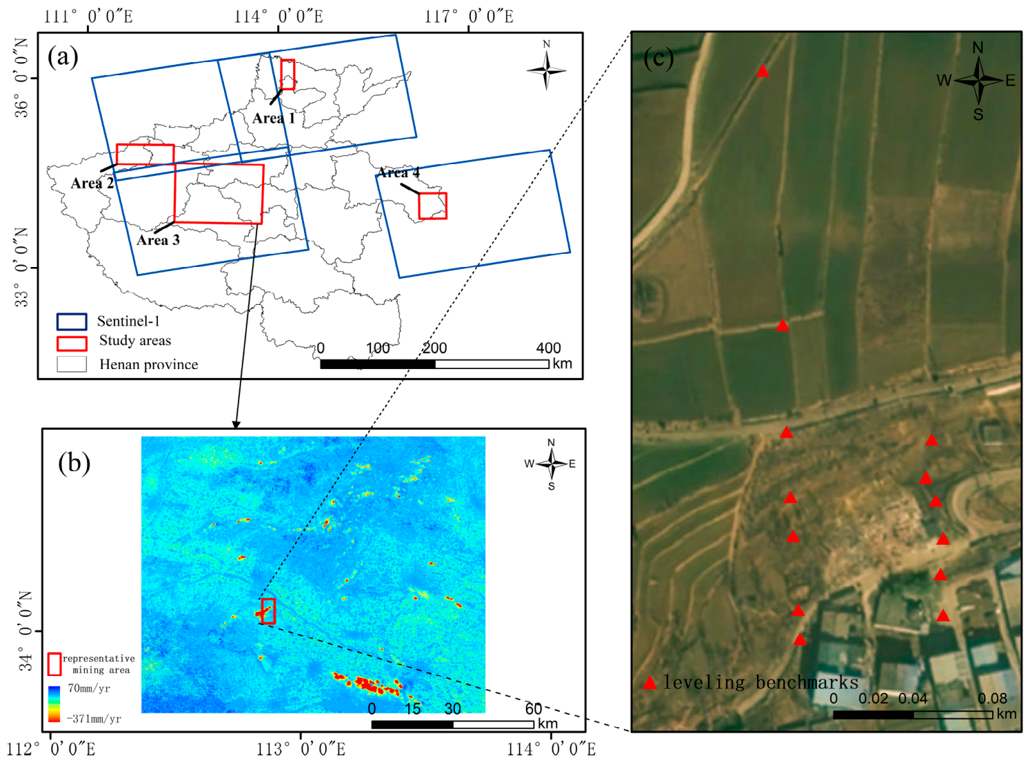
To mitigate cross-track mosaicking errors, enhance the comparability of spatiotemporal sequences, and fully account for factors such as the spatial agglomeration of mining areas, differences in geological and geomorphological units, and the coverage and orbital homogeneity of InSAR data, this study divides the concentrated coal mining areas in Henan Province into four study areas, as illustrated in Figure 1. Subsidence inversion and subsequent factor analyses are conducted separately within these four areas to ensure the capture of spatial heterogeneity. Study Area 1 covers approximately 3323 km² and is located in northern Henan Province, encompassing cities such as Hebi and Anyang within the piedmont zone at the southern foot of the Taihang Mountains. Its geomorphology is characterized by the development of proluvial–alluvial fan groups and frontal fault zones, with a moderate thickness of Quaternary loose deposits. Study Area 2 spans approximately 2976 km² in western Henan Province, including Sanmenxia and western Luoyang, and is situated at the northern margin of the Qinling and Funiu Mountains. This area features strongly dissected mountainous terrain and complex tectonic activity, leading to significant variations in overburden structures and bedrock exposure conditions. Study Area 3, covering approximately 13,101 km², serves as the core intensive zone of coal mine distribution and extends across multiple cities, including Luoyang, Zhengzhou, Xuchang, and Pingdingshan. Its geomorphological features alternate between those of the Yellow River alluvial plain and low hills, characterized by thick Quaternary deposits, a relatively uniform structure, dense industrial parks, and a high level of urbanization. Study Area 4 is approximately 1706 km² and is located in eastern Henan Province, covering Shangqiu and other regions at the margin of the eastern Henan sedimentary basin. The terrain is flat with thick sedimentary layers, where soft soils and fine-grained deposits are widely distributed, exhibiting typical characteristics of a plain mining area.

2.2. Data

2.2.1. SAR Data

In this study, the Sentinel-1A satellite of the Copernicus Programme initiated by the European Space Agency (ESA) is employed as the data source for surface deformation monitoring. C-band Sentinel-1A ascending orbit data covering the primary mining areas in Henan Province from March 2017 to February 2025 are collected, operating in the Interferometric Wide Swath (IW) mode [51].

During differential interferometry processing, the Shuttle Radar Topography Mission (SRTM) 1 arc-second global Digital Elevation Model (DEM), featuring a spatial resolution of approximately 30 m, is selected to simulate and remove the topographic phase. The main parameters of the Sentinel-1A images are detailed in

Table 1. Main parameters of the Sentinel-1A data.

Parameter	Value
Pass direction	Ascending
Beam mode	IW
Polarization	VV
Wave band	C
Wavelength/cm	5.6
Monitored period	March 2017–February 2025

.

The number of Sentinel-1A images, paths, frames, and the latitude and longitude ranges used for each study area are presented in

Table 2. Sentinel-1A datasets and imaging-geometry parameters used in the four study areas.

Study Area	Number of Images	Path	Frame	Mean Incidence Angle (°)	Incidence-Angle Range (°)	Heading Angle (°)	Longitude and Latitude (°)
Area1	234	40	112	36.85	36.03–37.66	−13.11	113.11–114.03E, 35.20–35.56N
Area2	228	113	111	34.06	31.13–36.88	−13.06	111.46–112.35E, 34.63–34.95N
Area3	225	113	106	39.82	35.41–43.93	−12.97	112.38–113.74E, 33.70–34.65N
Area4	227	142	106	35.46	33.94–36.95	−12.97	116.22–116.65E, 33.78–34.18N

. The imaging-geometry parameters were extracted from the Sentinel-1A products corresponding to the four study areas. The satellite heading angle was obtained from the product metadata, while the LOS azimuth angle was extracted to evaluate the directional sensitivity of the vertical projection to east–west and north–south displacements. The resulting imaging-geometry parameters are summarized in Table 2.

2.2.2. Ancillary Data

To construct the explanatory-variable dataset for the XGBoost-SHAP analysis, multisource topographic, land-surface, vegetation, hydrological, and meteorological datasets were integrated. The selected variables included elevation, slope, aspect, land-cover type, the normalized difference vegetation index (NDVI), precipitation, and groundwater table depth.

Elevation was obtained from the 30 m Shuttle Radar Topography Mission digital elevation model (SRTM DEM), from which slope and aspect were derived. Land-cover information was obtained from the 30 m China Land Cover Dataset for 2020 (CLCD 2020). NDVI was derived from Landsat imagery and organized as a 12-day product at a spatial resolution of 30 m. These datasets were used to characterize the topographic setting, surface-cover conditions, and vegetation dynamics of the study areas.

Precipitation was represented by 12-day gridded products with a native spatial resolution of 1 km. Groundwater conditions were represented by monthly groundwater table depth data obtained from the Monthly Groundwater Level Grid Dataset of the China Region (2005–2022) [52,53], which also had a native spatial resolution of 1 km. Groundwater table depth (GW) was defined as the positive downward distance from the land surface to the groundwater table, expressed in meters. Thus, higher GW values indicated deeper groundwater conditions, whereas lower values indicated shallower groundwater conditions. The XGBoost-SHAP analysis was restricted to the common period from 2017 to 2022, during which the InSAR deformation observations and all explanatory datasets were simultaneously available. The InSAR results from 2023 to February 2025 were used only for deformation monitoring and spatiotemporal evolution analysis.

For auxiliary analysis of the relationship between mining activity and surface deformation, mining-rights data provided by the Henan Institute of Geological Research were integrated. The dataset contains the geographic locations and boundaries of the mining areas, together with the documented commencement times and effective mining periods of the corresponding mines. The mining-area boundaries were used to examine the spatial correspondence between the observed subsidence zones and mining activities, whereas the recorded mining commencement times were compared with the cumulative SBAS-InSAR deformation time series at representative monitoring points. The validation data consisted of leveling measurements acquired at 14 leveling benchmarks located in a representative mining area within Study Area 3. Repeated leveling surveys were conducted from 5 May 2023 to 20 July 2023, and the measurements were used for local validation of the SBAS-InSAR-derived deformation. The spatial distribution of these leveling benchmarks is shown in Figure 1, and the point information is summarized in

Table 3. Subsidence influencing factor analysis and auxiliary datasets.

	Dataset	Source	Parameters
Subsidence Monitoring	Mining Rights Data of Henan Province	Henan Institute of Geological Research	—
	Leveling Measurements (14 Leveling Benchmarks)	Henan Institute of Geological Research	5 May 2023–20 July 2023
Driving Factors Data	SRTM DEM	NASA	30 m
	Slope	SRTM DEM	30 m
	Aspect	SRTM DEM	30 m
	Land Cover Data of China 2020	Aerospace Information Research Institute, CAS	30 m
	NDVI	Landsat Imagery	30 m
	Precipitation	NASA	1 km
	Groundwater table depth	National Tibetan Plateau Data Center (TPDC)	1 km

.

All multisource environmental factors undergo rigorous resampling, projection transformation, and spatiotemporal matching to ensure high consistency with the InSAR subsidence data at the analytical scale. The subsidence driving factors and ancillary datasets utilized in this study are detailed in Table 3.

2.3. Methods

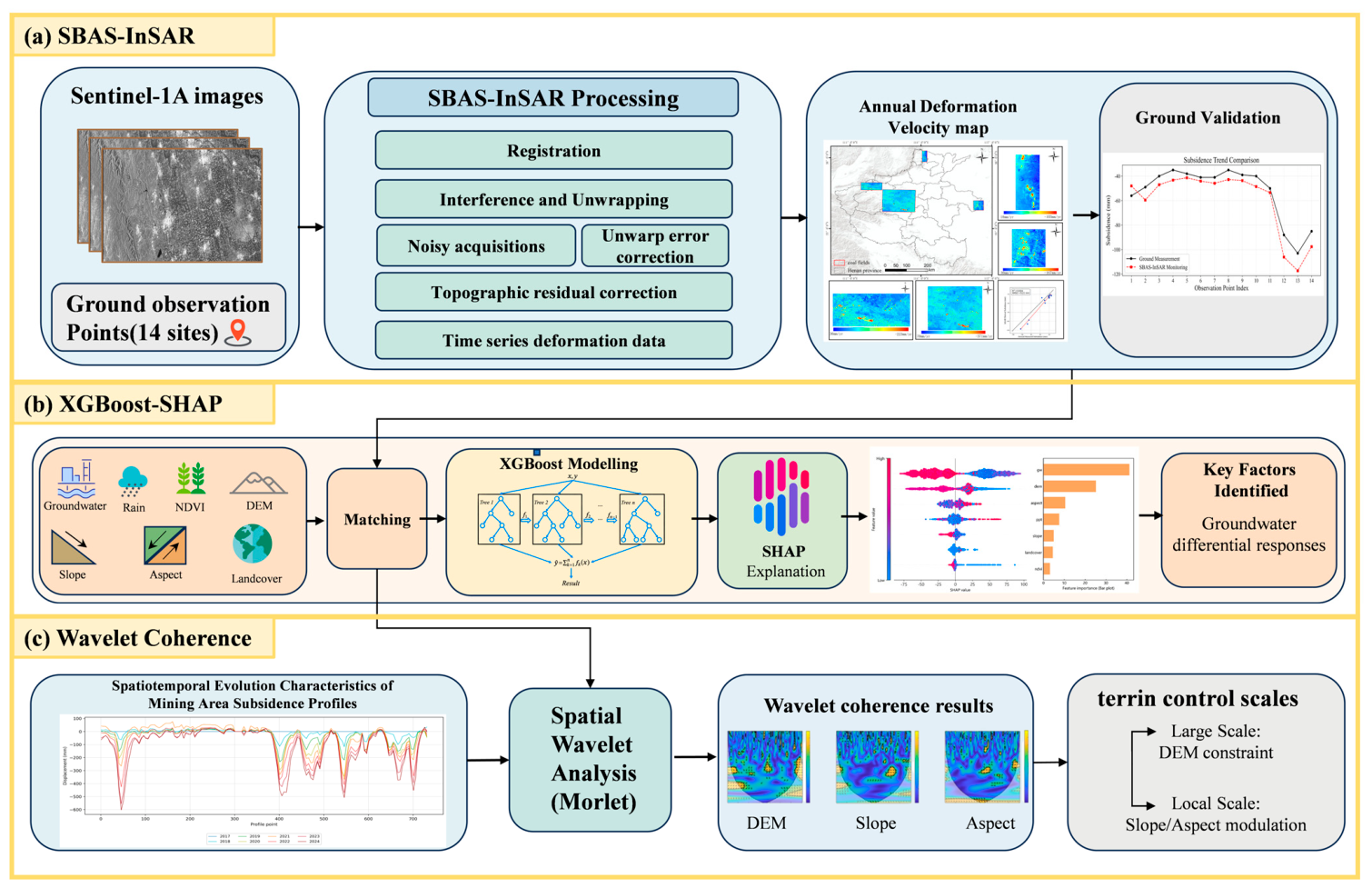
In this study, a method for surface subsidence monitoring and driving factor analysis that integrates multisource data is proposed. The methodological workflow is illustrated in Figure 2. The overall method consists of three main steps. First, SBAS-InSAR processing of the Sentinel-1A imagery was performed to derive surface deformation across the four study areas. A local validation was subsequently conducted within a representative mining area in Study Area 3 using measurements from 14 leveling benchmarks. Second, an XGBoost model and the SHAP explanation method are used to model the surface subsidence rate with environmental factors, including precipitation, groundwater table depth, the NDVI, the DEM, slope, aspect, and landcover. This modeling quantifies the relative explanatory contributions of the selected variables and characterizes their differential model-based response patterns among the study areas. Third, wavelet analysis employing the Morlet wavelet is applied to examine the spatial characteristics of subsidence along representative profiles. This step integrates the DEM, slope, and aspect sequences to identify scale-dependent spatial associations between topography and subsidence.

2.3.1. SBAS-InSAR Method

The SBAS-InSAR method [13] uses short spatiotemporal baselines to combine interferometric pairs, thereby reducing decorrelation effects and increasing the number of available interferograms. Each generated interferogram requires phase unwrapping. This technique divides the complete set of SAR images into several subsets where the spatiotemporal baselines between images within each subset are relatively short. Ultimately, all the subsets of the small baseline subsets are solved jointly. To mitigate atmospheric phase delays and the effects of spatiotemporal decorrelation, coherent point targets must be accurately identified, and high-precision image coregistration must be achieved. One image from the $N+1$ SAR images covering the same area is selected as the master image, and the remaining images are coregistered to it, generating a total of $M$ interferograms through combination. The variable $M$ satisfies the following relationship:

$${\displaystyle \frac{N+1}{2}}\le M\le {\displaystyle \frac{N\left(N+1\right)}{2}}$$

(1)

The j-th interferogram is formed by temporally combining acquisitions $t_a$ and $t_b$ ($t_a$ < $t_b$). After the flat-Earth effect and topographic phase are removed, the interferometric phase of any arbitrary point in the interferogram $j$ can be expressed by Equation (2):

$${\delta }_{{\phi }_j}={\phi }_{t_b}-{\phi }_{t_a}\approx {\displaystyle \frac{4\pi }{\lambda }}\left(d_{t_b}-d_{t_a}\right)+\Delta {\phi }_{top,j}+\Delta {\phi }_{atm,j}+\Delta {\phi }_{noise,j}$$

(2)

$\lambda$ denotes the central radar wavelength. The variables ${ d}_{t_a}$ and $d_{t_b}$ define the accumulated line-of-sight (LOS) displacements at acquisitions $t_a$ and $t_b$, respectively, relative to the reference baseline $t_0$. Furthermore, the phase contributions from residual topography, atmospheric delay, and decorrelation noise are parameterized as $\Delta {\phi }_{\mathrm{top},j}$, $\Delta {\phi }_{\mathrm{atm},j}$ and $\Delta {\phi }_{\mathrm{noise},j}$, respectively. By isolating the deformation signal through the compensation of these extraneous phase components, the final interferometric phase can be formulated as Equations (3) and (4).

$${\Delta \delta }_{{\phi }_j}={\phi }_{t_b}-{\phi }_{t_a}\approx {\displaystyle \frac{4\pi }{\lambda }}\left(d_{t_b}-d_{t_a}\right)$$

(3)

$$d_{t_b}-d_{t_a}={\upsilon }_i\left(t_b-t_a\right)$$

(4)

$v$ denotes the mean LOS deformation velocity spanning the temporal interval from $t_a$ to $t_b$. Accordingly, the relationship for the unwrapped differential phases is established through the matrix presented in Equation (5).

$$Av=\delta \phi$$

(5)

Because this study focuses on vertical subsidence in coal mining areas and the leveling measurements quantify vertical displacement, the LOS displacement was projected onto the vertical direction under the assumption that the deformation is predominantly vertical. According to Equation (6), the deformation in the radar line-of-sight direction was converted to approximate vertical subsidence, thereby generating the subsidence dataset used for the study area:

$$\Delta H={\displaystyle \frac{\Delta R}{cos\theta }}$$

(6)

where $\Delta H$ is the amount of subsidence, $\Delta R$ is the deformation in the LOS direction, and $\theta$ is the angle of incidence [54]. Because this conversion assumes that the horizontal displacement is negligible, a sensitivity analysis based on different horizontal-to-vertical displacement ratios was further conducted to evaluate the potential error associated with this assumption.

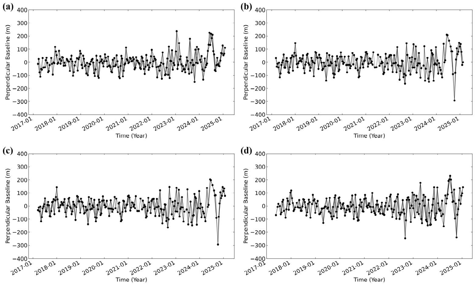
In this study, the SAR dataset is processed on the platform of the National Supercomputing Center in Zhengzhou using the open-source software packages ISCE2 (v2.6.3) and MintPy (v1.6.2). The ISCE2 package was deployed for the foundational processing of the SAR dataset, which included coregistration, interferometry, and unwrapping; the resulting spatiotemporal baseline distribution is presented in Figure 3. For the extraction of time series deformation, MintPy was applied. Interferometric pairs were generated using a temporal baseline threshold of 36 days and a perpendicular baseline threshold of 400 m. To improve the quality of the interferograms, a filtering coefficient of 0.7 was applied to suppress phase noise, and multilook factors of 2 and 10 were applied in the range and azimuth directions, respectively, to balance the signal-to-noise ratio and processing efficiency. We refined the InSAR measurements by filtering out tropospheric and topographic artifacts utilizing global atmospheric models (GAMs). Consequently, the long-term cumulative deformation and annual subsidence rates were derived for the period spanning March 2017 to February 2025.

For spatial matching between the leveling benchmarks and the SBAS-InSAR results, the coordinates of the leveling benchmarks and the SBAS-InSAR measurement points were first transformed into the same projected coordinate reference system. For each leveling benchmark, all valid SBAS-InSAR measurement points within a 50 m radius were identified, and their arithmetic mean was used to represent the local SBAS-InSAR deformation. If no valid SBAS-InSAR measurement points were available within 50 m, the search radius was extended to 100 m, and the arithmetic mean of all valid points within the expanded buffer was calculated. This buffer-based averaging strategy was adopted to reduce the influence of isolated anomalous InSAR measurements, residual geocoding uncertainty, and the spatial non-colocation between the leveling benchmarks and the SBAS-InSAR measurement points. The relatively small search radii were used to limit excessive spatial smoothing across the large deformation gradients commonly observed in mining areas [55,56]. For temporal alignment, the cumulative SBAS-InSAR deformation at the beginning and end of the leveling observation period from 5 May 2023 to 20 July 2023 was extracted or linearly interpolated from the SBAS-InSAR time series. The difference between these two cumulative deformation values was then compared with the leveling-derived vertical displacement.

2.3.2. Explainable Influencing Factor Analysis Based on the XGBoost-SHAP Model

Because the deformation characteristics and environmental settings differed among the four study areas, an independent XGBoost model was developed for each area using data from 2017 to 2022.

Each modeling record was defined as a pixel–date sample, representing one valid InSAR pixel at one Sentinel-1 acquisition date. The response variable was the cumulative vertically projected displacement from the first reference acquisition of the corresponding study area to the sample date. It was expressed in millimeters, with negative values indicating subsidence. Therefore, the response variable represented acquisition-date-specific cumulative deformation.

The explanatory variables consisted of four static predictors, including elevation, slope, aspect, and land-cover type, and three time-varying predictors, including NDVI, precipitation, and groundwater table depth. All datasets were transformed to a common coordinate reference system and aligned to a 30 m analytical grid. The native 1 km precipitation and groundwater table depth rasters were resampled to this grid using bilinear interpolation.

NDVI and precipitation were represented by 12-day products. Products whose nominal dates coincided with Sentinel-1 acquisition dates were matched directly. Otherwise, the nearest product within six days was used. Remaining internal gaps in the pixel-level time series were filled by linear interpolation based on the actual observation dates. Monthly groundwater table depth values were extracted after spatial resampling and temporally interpolated to the Sentinel-1 acquisition dates according to the actual calendar-day intervals between adjacent monthly observations [57]. Records containing missing response or predictor values after spatial and temporal matching were excluded from model fitting. The mining-rights data were not included as continuous predictors in the XGBoost models because they provided mining-area boundaries and documented mining periods but did not contain spatially and temporally continuous measures of mining intensity, such as working-face advancement, extraction volume, mining depth. Mining activity was therefore evaluated separately through its spatial and temporal correspondence with the observed deformation, whereas the XGBoost-SHAP analysis was used to characterize the relative explanatory contributions of the selected environmental and topographic variables within mining-affected areas.

For each study area, the samples were divided into training and validation subsets at a ratio of 70:30 using a random pixel-level split implemented with train_test_split (shuffle = True). To further evaluate the influence of spatial autocorrelation on model performance, an additional fivefold spatial block cross-validation was conducted independently for each study area. The 30 m analytical grid was partitioned into non-overlapping 1 km × 1 km spatial blocks according to the projected coordinates. Entire spatial blocks, including all pixel–date records located within the same block, were assigned to the same fold, thereby preventing observations from the same spatial unit from appearing simultaneously in the training and validation datasets. In each iteration, four spatial folds were used for model fitting, and the remaining fold was used for validation.

The 1 km block size was selected as a practical validation. Model performance was evaluated using R², RMSE, and MAE. The overall spatial cross-validation metrics were calculated from the combined out-of-fold predictions, whereas the mean and standard deviation of the fold-specific R² values were additionally reported to characterize performance variability among spatial folds. The search space comprises eight hyperparameters, as shown in

Table 4. Parameter space for XGBoost.

Parameters	Notes	Parameter Range
n_estimators	Number of base learners	{300, 500, 800, 1000}
learning_rate	Learning rate	{0.005, 0.01, 0.03, 0.05}
max_depth	Maximum depth of a tree	{3, 4, 5, 6}
subsample	Line sampling ratio	{0.7, 0.8, 0.9, 1.0}
colsample_bytree	Feature sampling ratio	{0.7, 0.8, 0.9, 1.0}
min_child_weight	Minimum Leaf Node Sample Weight	{1, 3, 5, 10}
reg_alpha	L1 Regularization Coefficient	{0, 0.01, 0.1, 1}
reg_lambda	L2 Regularization Coefficient	{0.5, 1, 2, 5}

.

Model performance was evaluated using the coefficient of determination (R²), RMSE, and mean absolute error (MAE). These metrics were calculated for the validation subsets, and the mean and standard deviation obtained from fivefold cross-validation were also reported to assess performance stability across different data partitions. Because separate models were fitted to the four study areas, cross-regional interpretation focused primarily on the relative ranking and direction of feature effects rather than on direct comparisons of unstandardized absolute SHAP magnitudes across models.

The Shapley Additive exPlanations method quantifies the contribution of each variable. Originating from cooperative game theory, SHAP computes the contribution of each independent variable to the dependent variable alongside the interactions among features, accommodating potential synergistic effects. The formulation of the Shapley value is defined as follows:

$${\mathsf{\varphi }}_j\left(\mathsf{\nu }\right)=\sum _{S\subseteq \{1,\dots ,p\}\setminus \left\{j\right\}}{\displaystyle \frac{\left|S\right|!\left(p-\left|S\right|-1\right)!}{p!}}\backslash big\left({\mathsf{\nu }}_x\left(S\cup \left\{j\right\}\right)-{\mathsf{\nu }}_x\left(S\right)\backslash big\right)$$

(7)

$S$ denotes a subset of the total $p$ features employed by the model, $x$ represents the input vector of the specific instance being evaluated, and ${\nu }_x\left(S\right)$ corresponds to the prediction conditioned exclusively on the features within $S$. The generation of SHAP summary and dependence plots allows for the quantitative analysis of the positive and negative contribution directions, as well as the marginal effects of each factor on subsidence.

2.3.3. Analysis of Topographic Factors in Coal Mining Areas Based on XWT and WTC

To investigate the scale-dependent spatial associations between surface subsidence and key topographic factors across multiple spatial scales, this study incorporates the cross-wavelet transform (XWT) and wavelet coherence (WTC) [58]. This methodology effectively identifies the common spatial-scale characteristics of two nonstationary spatial sequences and visually represents their relative spatial phase relationships through the phase spectrum. The continuous wavelet transform (CWT) serves as the theoretical basis for cross-wavelet analysis [59]. Mathematically, for an arbitrary discrete spatial sequence, its CWT is expressed through the convolution of the data sequence with a selected mother wavelet:

$$W_n^X\left(s\right)=\sqrt{{\displaystyle \frac{\delta t}{s}}}{\displaystyle \sum _{n^{\prime }=0}^{N-1}}{x}_{n^{\prime }}{\psi }^{*}\left[{\displaystyle \frac{\left(n^{\prime }-n\right)\delta t}{s}}\right]$$

(8)

where $s$ is the scale factor corresponding to the spatial scale, $\delta t$ is the spatial interval between adjacent points along the profile, $n$ is the spatial translation parameter, and ${\psi }^{*}$ represents the complex conjugate. In this study, the Morlet wavelet was employed as the basis function. Its localization properties in both the spatial-position and scale domains are suitable for analyzing spatial sequences of surface subsidence and topographic factors. Building upon this, the cross-wavelet transform allows the common high-energy regions of two spatial sequences to be analyzed in the spatial-scale domain. Their cross-wavelet spectrum is formulated as follows [60]:

$${ W}_n^{XY}\left(s\right)=W_n^X\left(s\right)W_n^Y(s{)}^{*}$$

(9)

where $W_n^X\left(s\right)$ is the wavelet transform of spatial sequence $X$and $W_n^Y(s{)}^{*}$ is the complex conjugate of the wavelet transform of spatial sequence $Y$. A larger cross-wavelet power indicates stronger common spatial variability between the two sequences at the corresponding spatial position and scale. Because the cross-wavelet transform may be influenced by high-energy values in an individual sequence, the wavelet coherence spectrum was further introduced to evaluate the local spatial association between the two sequences [61]. The wavelet coherence coefficient $R_n^2\left(s\right)$, which functions as a local correlation coefficient in the distance–scale domain, is defined as follows:

$$R_n^2\left(s\right)={\displaystyle \frac{\left|S\right(s^{-1}{W}_n^{XY}\left(s\right)){|}^2}{S\left(s^{-1}|W_n^X\left(s\right){|}^2\right)\cdot S\left(s^{-1}|W_n^Y\left(s\right){|}^2\right)}}$$

(10)

where $S$ is a smoothing operator. The value of $R_n^2$ ranges from 0 to 1, with values approaching 1 indicating a stronger local association between the two spatial sequences at the corresponding profile position and spatial scale. Regions satisfying the 95% confidence-level test are delineated by thick black solid lines generated through Monte Carlo simulations [62]. Furthermore, the phase arrows in the XWT and WTC spectra represent the relative spatial phase relationships between the two sequences along the profile direction. It should be emphasized that wavelet coherence functions as a localized correlation measure in the distance–scale domain. A significant coherence region indicates that the two spatial sequences exhibit related spatial variations within a specific profile segment and spatial scale. Following the identification of strongly correlated factors, representative spatial profile lines are established in the typical subsidence trough areas within the mining region. The spatial distribution data of subsidence and topographic factors, including the DEM, slope, and aspect, are extracted along these profile lines. Spatial correlation analysis subsequently examines the controlling influence of topographic variations on the morphology of the subsidence trough across different spatial distances, thereby elucidating the causes of heterogeneity in the spatial distribution of subsidence. In this study, the Morlet wavelet was selected as the mother wavelet because of its good localization capability in both the spatial-position and scale domains. The scale resolution was set to $dj=1/12$, and the minimum scale was defined as twice the spatial interval between adjacent points along the profile sequence. The wavelet scales were converted into equivalent spatial distances according to the spatial interval of the profile sequence and the scale-to-wavelength relationship of the Morlet wavelet, and the resulting spatial scales were expressed in meters or kilometers. The significance level of the wavelet coherence spectrum was tested against a first-order autoregressive spatial background spectrum. The first-order spatial autocorrelation coefficients of the two input spatial sequences were estimated automatically by the toolbox. A Monte Carlo simulation with 300 surrogate spatial sequences was used to estimate the 95% confidence level. Regions exceeding the 95% confidence level are marked by thick black contours in the WTC spectra, whereas the cone of influence was used to identify regions where edge effects may affect the reliability of the coherence estimates.

3. Results

3.1. Surface Subsidence Monitoring and Local Validation in the Study Areas

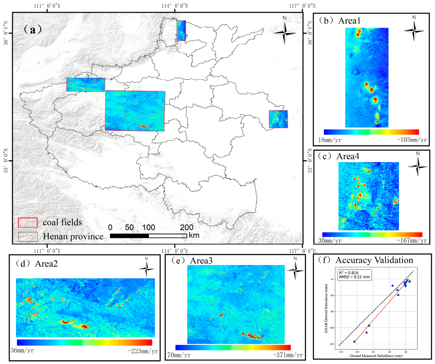
The surface subsidence rates of coal mines in Henan Province and the corresponding local validation results derived from the SBAS-InSAR inversion between March 2017 and February 2025 are presented in Figure 4a–f, respectively.

A detailed analysis of Study Areas 1 through 4 reveals that the deformation rate in Study Area 1 (Figure 4b) primarily ranges from 18 mm/yr to −103 mm/yr. Spatially, this manifests as multiple independent subsidence troughs distributed discretely along specific directions, featuring clear boundaries at the subsidence centers. Study Area 2 (Figure 4d) peaks at a subsidence velocity of −223 mm/yr, with anomalous subsidence zones expanding continuously along the mining area. These local regions interconnect to form a distinct strip-like subsidence distribution. Study Area 3 (Figure 4e) records the most severe deformation signals during the monitoring period, with rates spanning from 70 mm/yr to −371 mm/yr, forming a vast and continuous deep subsidence center in the regional core. Study Area 4 (Figure 4c) displays a peak settlement rate of −167 mm/yr, which is dominated by a planar subsidence zone with local patchy anomalies. The subsidence range of Study Area 4 is more continuous than that of Study Area 1, whereas the overall intensity is weaker than the intensities of Study Areas 2 and 3 are.

The surface subsidence rates in the coal mining areas of Henan Province exhibit highly heterogeneous spatial distributions. Across the province, subsidence areas are primarily concentrated in densely distributed coal mine regions in northern, central, and eastern Henan. Non-subsidence or weak subsidence areas are widely distributed around the periphery of mining areas and exhibit strong spatial consistency with coalfield boundaries and the range of influence of mining activities. The high subsidence areas generally display a spatial pattern that combines patchy, strip-like, and subsidence troughs. The extent, intensity, and connectivity of subsidence centers vary significantly among different mining areas, highlighting distinct regional differences.

To quantitatively evaluate the reliability of the SBAS-InSAR monitoring results, a local validation was conducted within a representative mining area in Study Area 3 using 14 leveling benchmarks surveyed from 5 May to 20 July 2023. The SBAS-InSAR-derived vertically projected displacements were compared with the corresponding leveling-derived vertical displacements at the benchmark locations.

As shown in Figure 4f, linear regression yielded an $R^2$ of 0.816 and an RMSE of 9.22 mm. The observations were generally distributed close to the regression line, indicating good agreement between the two measurement datasets at the selected benchmarks during the validation interval.

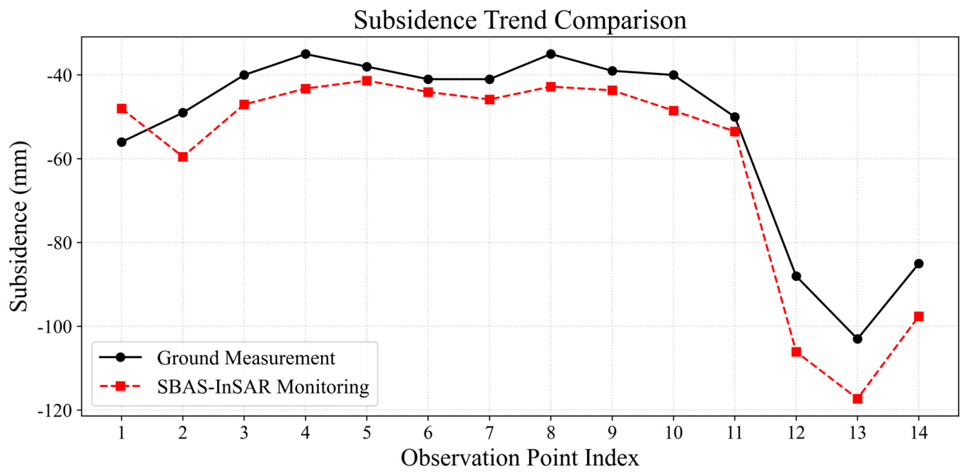
To further examine the consistency between the two datasets, Figure 5 compares the leveling-derived vertical displacement with the corresponding SBAS-InSAR-derived vertically projected displacement at the 14 leveling benchmarks. The black solid line represents the leveling measurements, whereas the red dashed line represents the matched SBAS-InSAR results. The deformation remains relatively stable from benchmarks 1 to 11, with most displacement values ranging from approximately −35 to −60 mm. From benchmark 12 onward, both curves exhibit a consistent downward trend and reach their largest subsidence magnitudes at benchmark 13. The leveling-derived vertical displacement at this benchmark is approximately −105 mm, whereas the corresponding SBAS-InSAR-derived displacement is approximately −117 mm. Both curves subsequently show a slight rebound from benchmark 13 to benchmark 14. Despite local numerical differences at benchmarks experiencing relatively large deformation, the two datasets exhibit consistent overall variation patterns.

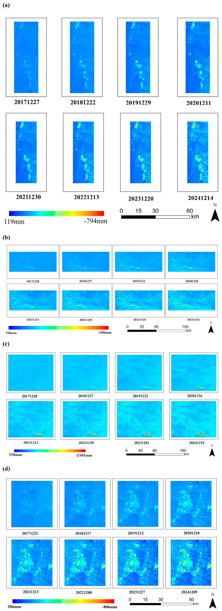
On the basis of the SBAS-InSAR monitoring results, the cumulative subsidence in the coal mining areas of Henan Province between 2017 and 2025 clearly evolves spatiotemporally. The spatiotemporal evolution characteristics of the four study areas are shown in Figure 6, with subplots (a) through (d) detailing the total accumulated settlement for Study Areas 1 to 4, respectively.

A comparison of the cumulative subsidence across the study areas reveals that Study Area 3 (Figure 6c) experienced the most significant subsidence intensity during the monitoring period. It reaches a maximum cumulative subsidence of −2101 mm and forms a large and continuous subsidence basin. The central area has high subsidence values and the broadest impact range, indicating that this region has experienced the strongest influence from mining activities. Study Area 2 (Figure 6b) follows, with a maximum subsidence of −1456 mm. Multiple subsidence centers are distributed along the mining area strike, indicating a certain degree of serial connection. In contrast, Study Areas 1 (Figure 6a) and 4 (Figure 6d) display relatively weaker cumulative deformations, with maximum cumulative subsidence values of −794 mm and −806 mm, respectively. Study Area 1 manifests primarily as multiple dispersed local subsidence points with weak spatial continuity in deformation. Study Area 4 features mainly patchy deformation with relatively discrete subsidence areas. Both areas exhibit minor local positive deformation signals, whereas overall, negative deformation remains dominant.

The surface deformation in the study area is dominated by subsidence (Figure 6). As mining activities continue, the range of negative deformation expands annually, and the subsidence amplitude increases steadily. This process shows a clear cumulative enhancement trend and eventually evolves into large-scale, continuously distributed subsidence basins in certain mining areas. A comparison of cumulative subsidence maps across different years reveals that the locations of subsidence centers generally remain stable, whereas the subsidence intensity continuously increases. This confirms that surface subsidence is characterized by significant continuous cumulative properties during the monitoring period.

In addition to subsidence, minor positive deformation areas can be identified in each study area, as shown in Figure 6. These areas appear as local, scattered patches of slight uplift. In terms of spatial patterns, compared with the subsidence areas, the uplift areas generally have small sizes, weak continuity, and significantly lower amplitudes. They do not form concentrated and contiguous distributions equivalent to those of the subsidence basins. With respect to temporal changes, the uplift signals lack the continuous expansion and enhancement trends observed in the subsidence areas and primarily present local fluctuation characteristics. Therefore, the dominant process of cumulative deformation in the study area remains mining-induced subsidence, with local uplift acting merely as an associated secondary deformation phenomenon. These local uplift signals may be associated with groundwater level recovery caused by rainfall recharge, irrigation return flow, or reduced local drainage, which can increase pore water pressure and reduce effective stress in shallow unconsolidated sediments, thereby inducing slight elastic expansion or rebound. In addition, stress redistribution around mined-out areas and the margins of subsidence troughs may also produce localized rebound, particularly in zones with relatively large deformation gradients. Therefore, the observed local uplift areas may reflect the combined influence of hydrogeological recharge and mining-related stress adjustment.

To further quantify the deformation characteristics of the four study areas, the annual deformation rate, cumulative displacement, high-subsidence area, and number of major subsidence centers are summarized in

Table 5. Statistical summary of the annual deformation rate, cumulative displacement, high-subsidence area, and major subsidence centers in the four study areas.

Study Area	Min Annual Rate (mm/yr)	Max Annual Rate (mm/yr)	Median Annual Rate (mm/yr)	Maxcumulative Subsidence (mm)	Median Cumulative Displacement (mm)	High-Subsidence Area (km2)	High-Subsidence (%)	Main Centers
Area 1	−103	18	−4.73	−794	−16	15.55	1.57	5
Area 2	−223	36	−7.12	−1456	−51	66.49	2.34	11
Area 3	−371	70	−4.15	−2101	−33	209.85	1.60	29
Area 4	−167	30	−0.28	−806	3	61.67	3.51	16

. Negative values indicate subsidence. The minimum annual deformation rate varied from −103 mm/yr in Area 1 to −371 mm/yr in Area 3, indicating that Area 3 experienced the strongest deformation intensity during the monitoring period. The maximum cumulative subsidence also occurred in Area 3, reaching 2101 mm, followed by Area 2 (1456 mm), Area 4 (806 mm), and Area 1 (794 mm). In contrast, the median annual deformation rates were much lower in magnitude than the extreme values in all four areas, suggesting that severe subsidence was spatially concentrated in localized mining zones rather than uniformly distributed across each study area. High-subsidence areas, defined as pixels with annual deformation rates ≤ −30 mm/yr, covered 15.55 km² in Area 1, 66.49 km² in Area 2, 209.85 km² in Area 3, and 61.67 km² in Area 4, corresponding to 1.57%, 2.34%, 1.60%, and 3.51% of the valid monitored areas, respectively. Major subsidence centers were identified as eight-neighbor-connected high-subsidence patches with areas ≥ 1 km². According to these criteria, Area 3 contained the greatest number of major subsidence centers (29), followed by Area 4 (16), Area 2 (11), and Area 1 (5). These statistics indicate that Area 3 had the strongest subsidence intensity and the largest high-subsidence area, whereas Area 4 had the highest proportion of high-subsidence pixels within its monitored area.

It should be noted that the deformation values reported in this section were obtained by projecting the Sentinel-1 line-of-sight displacement onto the vertical direction under the assumption that horizontal motion is negligible. However, this assumption may not be fully valid in active mining areas, particularly near the margins of subsidence troughs where deformation gradients are steep and horizontal displacement may become appreciable. Therefore, the reported deformation magnitudes should be interpreted as approximate vertically projected displacements rather than strictly decomposed vertical displacements, and they may contain projection-related uncertainty caused by unaccounted horizontal motion.

3.2. Relationships Between Mining Activities and Land Subsidence

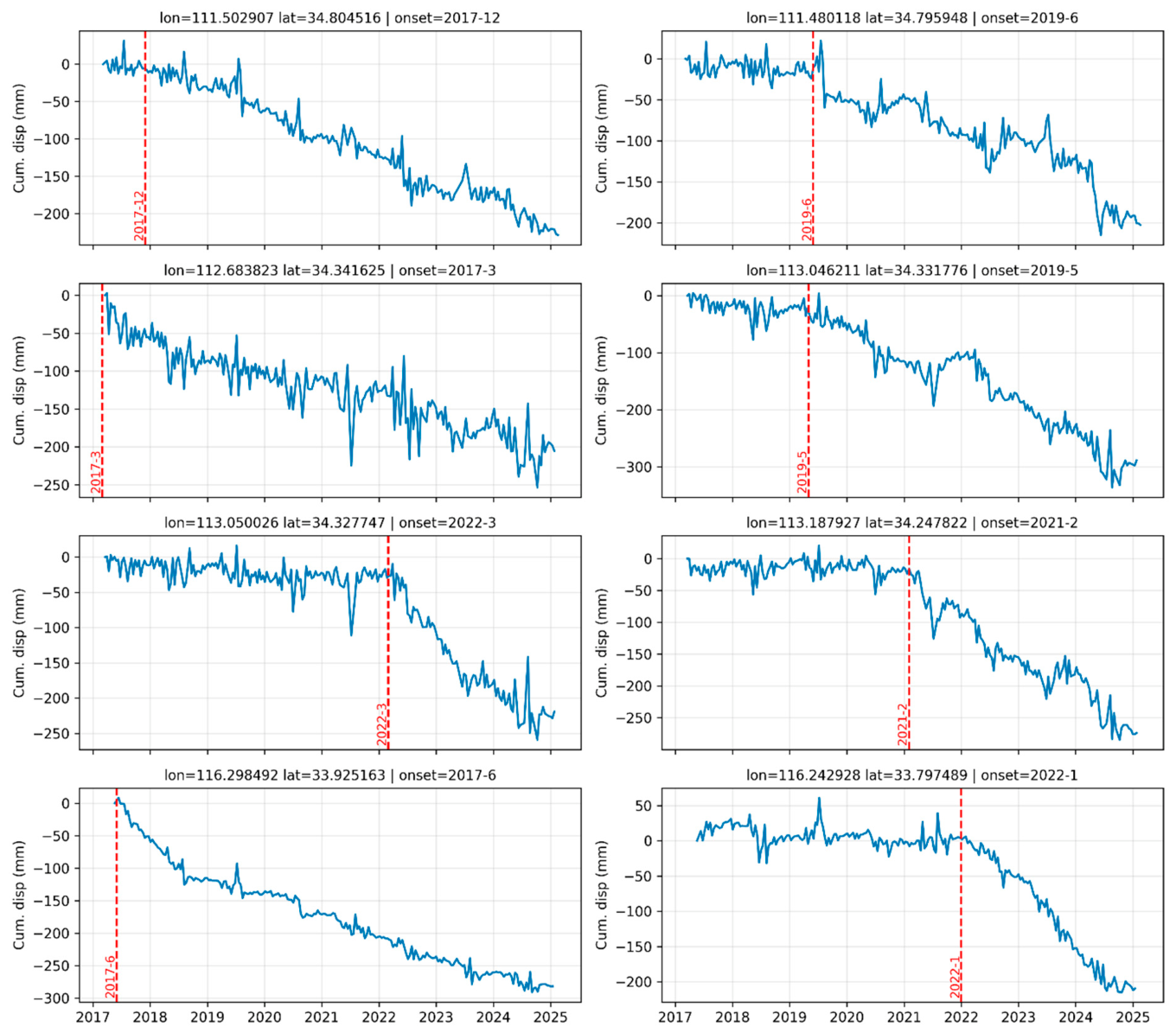
Mining activities in coal mine areas generally constitute the primary factor inducing surface subsidence. In this study, SBAS-InSAR is used to obtain multitemporal cumulative subsidence curves, and the subsidence records of typical monitoring points are compared with the mining periods documented in mining rights data. These comparison results are shown in Figure 7. The typical monitoring points clearly exhibit temporal correspondence between their subsidence time series and the effective periods of mining activities. Before mining activities commence (left of the red dashed line), the cumulative subsidence curves of most monitoring points generally remain flat with minor fluctuations. Upon entering the effective mining period, the curves universally display a downward accelerating trend alongside continuously increasing cumulative subsidence. The slopes of the curves at certain points become significantly steeper. Although the subsidence amplitudes of representative points across different study areas vary, their curve trajectories share a common transition from slow deformation to continuous subsidence. This consistent temporal pattern provides strong evidence that mining activities serve as crucial driving factors for subsidence evolution.

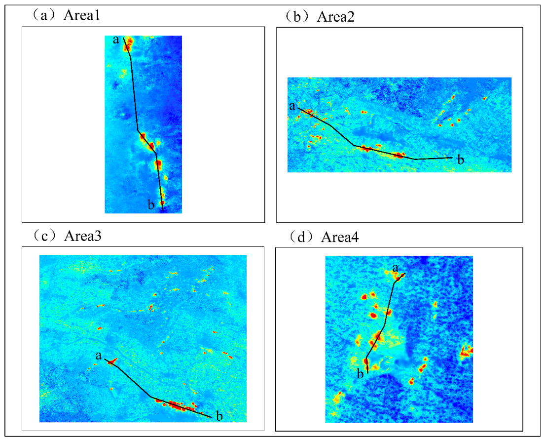
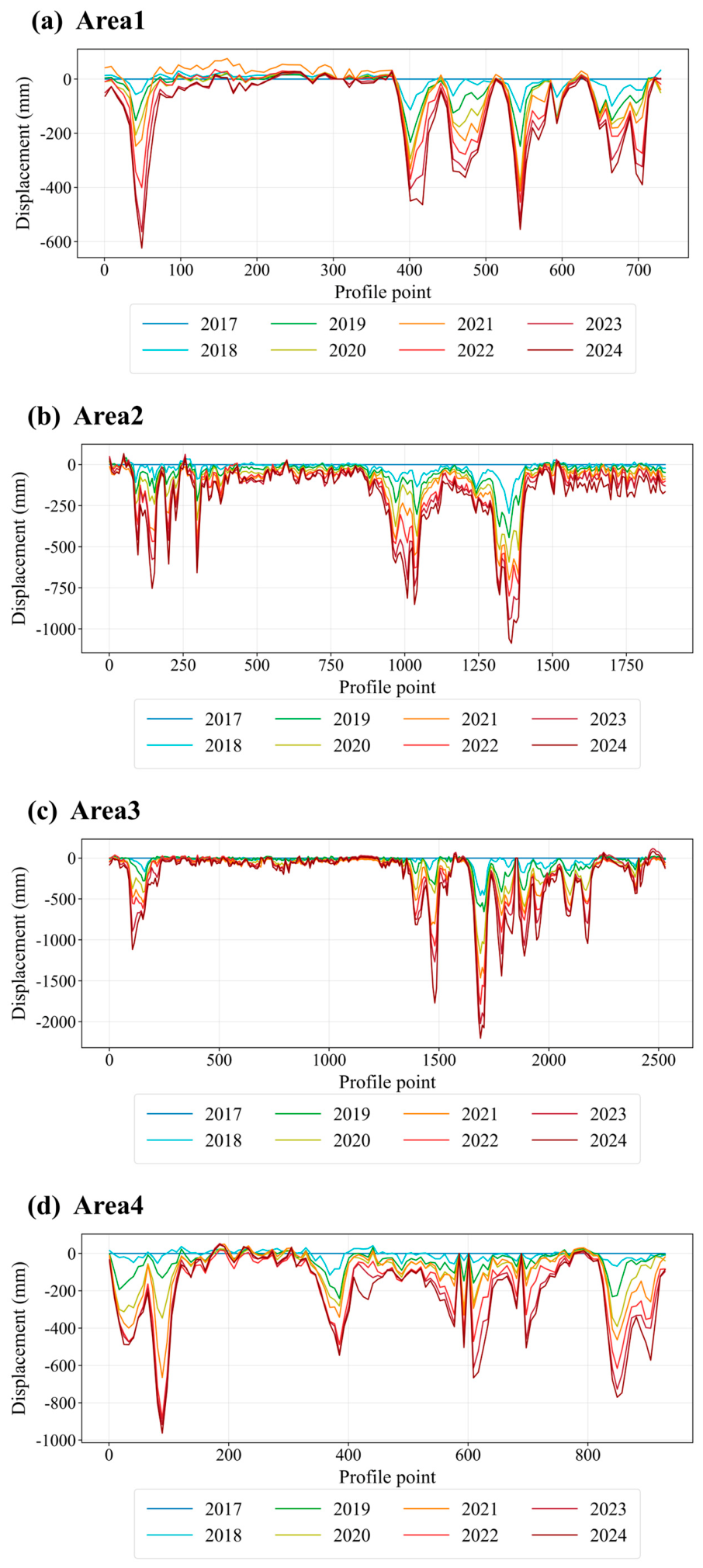
To further elucidate the detailed spatiotemporal evolution characteristics of mining subsidence, typical profile lines traversing the primary subsidence troughs within Study Areas 1 to 4 are established in this study. The locations of these profile lines, which are oriented from point a to point b, are shown in Figure 8a–d, respectively. In this study, cumulative subsidence profile data aggregated at annual intervals between March 2017 and February 2025 are extracted. Each annual dataset forms a line representing the subsidence conditions along the profile. The temporal evolution results of these profiles are presented in Figure 9. To avoid overinterpreting isolated local fluctuations in the profile curves, the independently validated RMSE of 9.22 mm obtained from the comparison between SBAS-InSAR results and leveling measurements was used as a reference uncertainty level. The profile analysis focused mainly on robust deformation features that persist across multiple annual profiles, including the progressive deepening of subsidence centers and the continuous expansion of subsidence ranges. The profile analysis clearly demonstrates the differentiated subsidence morphologies across various mining areas under the combined effects of geological conditions and mining intensity. Surface subsidence in the coal mining areas of Henan Province exhibits significant spatial heterogeneity. The profile curve of Study Area 1 (Figure 9a) indicates that local depressions deepen annually. This area contains numerous subsidence centers with narrow individual widths. The profile curve of Study Area 2 (Figure 9b) presents a continuous, broad, and gentle downward concavity with clear connections between subsidence centers. The profile in Study Area 3 (Figure 9c) is the most prominent, where the curve forms a deep and wide main subsidence trough in the central region. The central depth and influence width of this trough increase synchronously over time. The overall fluctuation of the profile in Study Area 4 (Figure 9d) is relatively gentle, yet multiple local low-value subsidence segments that intensify annually remain identifiable. Overall, the profiles of the four study areas consistently demonstrate a spatiotemporal evolution pattern characterized by the gradual deepening of subsidence centers and the continuous expansion of subsidence ranges. Minor rebound points and short-wavelength fluctuations along the profiles may be related to residual atmospheric noise, decorrelation, interpolation uncertainty, local surface disturbance, or secondary deformation processes. Because these signals are local, weak, and discontinuous, they were regarded as secondary fluctuations rather than dominant deformation features.

3.3. Analysis Results of the Subsidence Driving Factors Based on SHAP

3.3.1. Predictive Performance of the XGBoost Models

The independently trained XGBoost models achieved high performance under the random pixel-level validation scheme, with validation R² values ranging from 0.894 to 0.980, RMSE values ranging from 10.10 to 45.88 mm, and MAE values ranging from 6.21 to 32.89 mm (

Table 6. Random validation and 1 km spatial fivefold cross-validation performance of the independently trained XGBoost models.

Study Area	Random Validation R2	Random RMSE (mm)	Random MAE (mm)	Overall Spatial CV R2	Spatial CV RMSE (mm)	Spatial CV MAE (mm)	Fold Specific R2 (mean ± SD)
Area 1	0.980	10.10	6.21	0.841	28.48	17.51	0.834 ± 0.063
Area 2	0.942	17.56	11.74	0.793	33.17	22.18	0.785 ± 0.071
Area 3	0.968	19.55	14.05	0.682	61.63	44.29	0.665 ± 0.096
Area 4	0.894	45.88	32.89	0.626	86.18	61.78	0.604 ± 0.112

). Area 1 achieved the highest random-validation performance, whereas Area 4 exhibited the largest absolute prediction errors. These random-validation results primarily represent the ability of the models to reproduce deformation patterns within each study area when spatially adjacent observations may occur in both the training and validation subsets.

Under the stricter 1 km spatial block cross-validation scheme, model performance decreased in all four study areas. The overall out-of-fold R² values were 0.841, 0.793, 0.682, and 0.626 for Areas 1–4, respectively. The corresponding RMSE values were 28.48, 33.17, 61.63, and 86.18 mm, while the MAE values were 17.51, 22.18, 44.29, and 61.78 mm. The fold-specific mean R² values were 0.834 ± 0.063, 0.785 ± 0.071, 0.665 ± 0.096, and 0.604 ± 0.112, respectively.

Compared with the random pixel-level validation, the spatial cross-validation R² values decreased by 0.139–0.286, accompanied by increases in RMSE and MAE. This decline confirms that random pixel-level splitting produced relatively optimistic performance estimates because neighboring observations shared spatially autocorrelated information. Nevertheless, all spatial cross-validation R² values remained positive and above 0.62, indicating that the models retained meaningful predictive capability when evaluated on spatially separated blocks. Areas 1 and 2 exhibited stronger spatial generalization, whereas Areas 3 and 4 showed larger prediction errors and greater fold-to-fold variability, suggesting stronger spatial heterogeneity and more limited transferability among local spatial units. Therefore, the random-validation results are interpreted as within-area fitting performance, whereas the spatial cross-validation results provide a more conservative estimate of spatial generalization.

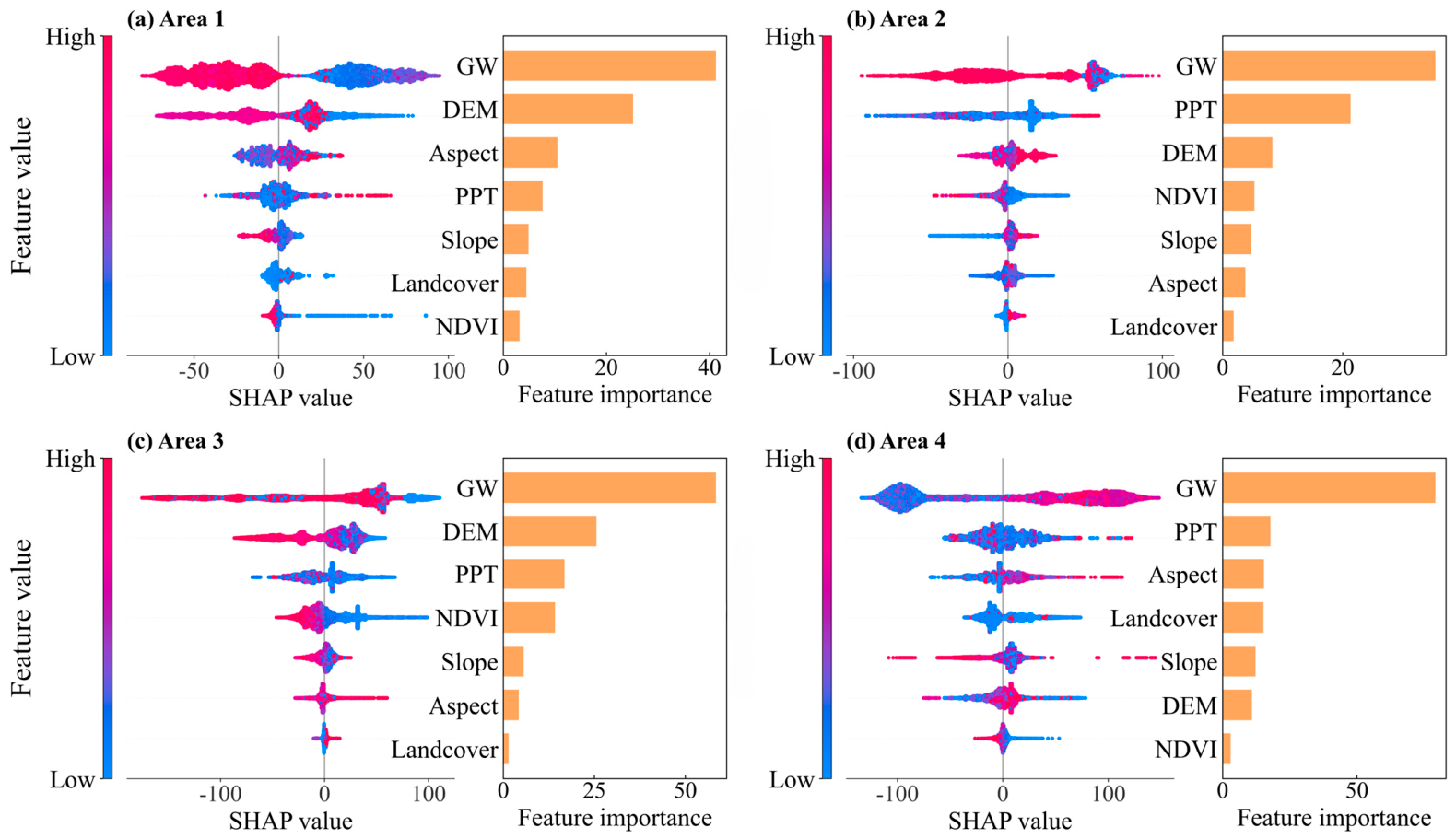
Mining activity is the fundamental physical driver of subsidence in coal mining areas. Within this context, selected hydrological, topographic, vegetation, and surface-cover variables may further modulate the spatial heterogeneity of mining-induced deformation. On the basis of the SHAP attribution of the XGBoost model, Figure 10a–d presents the relative contribution rankings of these variables. Although the explanatory structures are somewhat consistent across the four study areas, clear regional differences exist in feature rankings, contribution magnitudes, and effect directions. Overall, groundwater table depth represents the most important measurable explanatory factor within the selected variables in the four fitted models. Precipitation, elevation, and the related topographic variables provide secondary explanatory contributions, whereas aspect, slope, landcover, and NDVI generally show lower contributions, although their relative importance varies among the study areas.

In Study Area 1 (Figure 10a), the feature importance ranking is GW > DEM > aspect > PPT > slope > landcover > NDVI. The mean absolute SHAP value of GW is significantly greater than those of the other variables, giving it the highest relative explanatory contribution among the selected variables. DEM is the variable with the second-highest relative explanatory contribution. Aspect and PPT contribute to some extent but are substantially lower than the top two factors are, while the importance of slope, landcover, and the NDVI remains relatively low. The feature importance ranking in Study Area 2 (Figure 10b) is GW > PPT > DEM > NDVI > slope > aspect > land cover. Compared with that in other regions, the importance of PPT increases significantly in this area, ranking second only to GW. The contribution of the DEM remains high but is lower than that in Study Area 1. The contributions of the NDVI, slope, and aspect are comparable, whereas landcover remains the lowest. In Study Area 3 (Figure 10c), the feature importance ranking is GW > DEM > PPT > NDVI > slope > aspect > landcover. The overall structure of this area closely resembled that of Study Area 1, with GW yielding the greatest contribution, followed by DEM and PPT. Although the importance of the NDVI slightly increased compared with that in Study Area 2, it still acted as a medium to low contributing factor. The mean absolute SHAP values for slope, aspect, and landcover are relatively low. The feature importance ranking in Study Area 4 (Figure 10d) is GW > PPT > aspect > landcover > slope > DEM > NDVI. This area clearly differs from the first three regions. Although GW remains at the highest level, the importance of the DEM decreases significantly. The contributions of aspect and landcover increase to the third and fourth positions, respectively, whereas the NDVI remains the variable with the lowest contribution.

The SHAP scatter distributions further reveal regional differences in the effect directions of each factor. Since the subsidence values are negative, a negative SHAP value indicates that the variable drives the model output toward a more negative direction, which corresponds to enhanced subsidence. Conversely, a positive SHAP value indicates weakened subsidence. In Study Areas 1–3, high GW values, representing greater groundwater table depths, are primarily associated with negative SHAP values, whereas low GW values, representing shallower groundwater tables, are mainly associated with positive SHAP values. This distribution indicates that a greater groundwater depth is more likely to correspond to stronger subsidence, whereas a shallower groundwater depth generally results in the relative suppression of subsidence. In Study Area 4, low GW values, representing shallower groundwater tables, are mainly associated with negative SHAP values, whereas high GW values are more frequently associated with positive SHAP values. This implies that a shallower groundwater depth in this area is more prone to inducing stronger subsidence. DEMs and PPTs also exhibit evident regional differences. In Study Areas 1 and 3, the DEM contributes strongly, and its high values mostly correspond to negative SHAP values. In Study Area 4, both the SHAP distribution range and the importance of the DEM weaken significantly. PPT ranks second in both Study Area 2 and Study Area 4, which demonstrates its stronger explanatory power in these two regions. The overall contributions of aspect, slope, landcover, and NDVI are relatively low, but the importance of aspect and landcover increases noticeably in Study Area 4.

Overall, the SHAP based attribution structures across the four study areas display significant spatial heterogeneity. Groundwater provides the highest relative explanatory contribution among the selected variables, but its effect direction clearly varies by region. The relative importance of the changes in the DEM and PPT among the study areas, whereas the effects of aspect and landcover become more pronounced in specific geological and geomorphological settings.

3.3.2. Associations Among Explanatory Variables and Robustness of SHAP Rankings

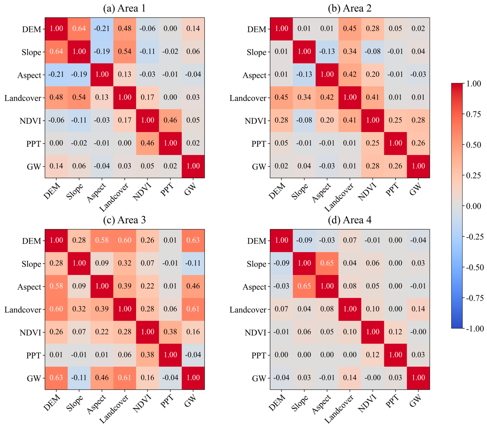
Figure 11 presents the association matrices of the explanatory variables in the four study areas. The maximum absolute coefficients were 0.637, 0.282, 0.628, and 0.646 in Areas 1–4, respectively. In Area 1, the strongest relationship was observed between DEM and slope ($r=0.637$), while NDVI and PPT showed a moderate positive relationship ($r=0.455$). Area 2 exhibited generally weak correlations among the continuous variables, with the maximum coefficient occurring between DEM and NDVI ($r=0.282$). In Area 3, moderate relationships were observed between DEM and GW ($r=0.628$), DEM and aspect ($r=0.582$), and aspect and GW ($r=0.464$). In Area 4, slope and aspect showed the strongest relationship ($r=0.646$), whereas the relationships among NDVI, PPT, and GW were weak. These results indicate that the explanatory variables contain some overlapping environmental information, but no strong pairwise correlation was detected.

The feature-ablation results are summarized in

Table 7. Feature-ablation results and consistency with SHAP rankings.

Area	Full R2	DEM	Slope	Aspect	Landcover	NDVI	PPT	GW	Rank ρ
Area 1	0.980	0.0264	0.0002	0.0321	0.0133	−0.0009	0.0280	0.1414	0.857
Area 2	0.942	−0.0007	−0.0015	−0.0001	0.0002	−0.0051	0.1534	0.1212	0.393
Area 3	0.968	0.0122	0.0026	0.0024	0.0006	−0.0007	0.0198	0.0816	0.750
Area 4	0.894	0.0467	0.0149	0.0182	0.0155	−0.0001	0.0625	0.1488	0.893

Note: R² denotes the coefficient of determination; ρ denotes Spearman rank correlation.

. The complete models achieved validation $R^2$ values of 0.9796, 0.9434, 0.9689, and 0.8937 in Areas 1–4, respectively. Removing GW caused the greatest reduction in model performance in Areas 1, 3, and 4, decreasing $R^2$ by 0.1414, 0.0816, and 0.1488, respectively. In Area 2, removing PPT resulted in the largest decrease in $R^2$ ($\Delta R^2=0.1534$), followed by GW ($\Delta R^2=0.1212$). PPT was also the second most influential variable in Areas 3 and 4 according to the ablation analysis.

The rankings derived from the feature-ablation analysis were generally consistent with the SHAP rankings for the principal variables. The Spearman rank correlations between the two rankings were 0.857, 0.393, 0.750, and 0.893 for Areas 1–4, respectively. Although Area 2 exhibited a relatively low overall rank correlation, GW and PPT were consistently identified as the two dominant variables by both methods. The differences mainly occurred among variables whose removal caused little or no decrease in validation performance. In Area 3, GW, DEM, and PPT constituted the three most influential variables under both approaches. These results demonstrate that the identification of the principal explanatory factors was robust, whereas the exact ordering of low-contribution variables was less stable.

3.4. Wavelet Coherence Analysis Results

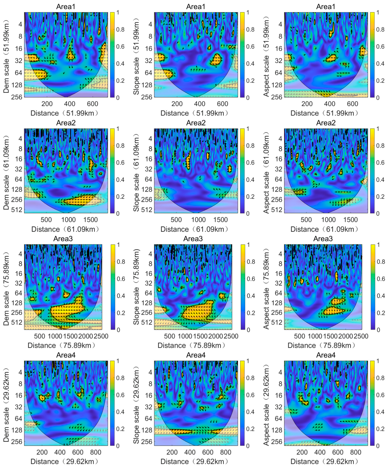
The XGBoost-SHAP attribution results presented in Figure 10 indicate that topographical factors hold high importance rankings in specific study areas alongside the explanatory contributions of groundwater and precipitation. To explore the relationship between topography and subsidence using wavelet analysis, profile lines are established across the four study areas to intersect the primary subsidence zones. The locations of these profile lines are shown in Figure 8. The coherence relationships between subsidence and topographical factors along the profile lines are shown in Figure 12. The wavelet coherence analysis along the profile lines reveals significant spatial scale-dependent characteristics between topographical factors, which include elevation, slope, and aspect, and surface subsidence. The spatial distribution of this coherence relationship is constrained by the continuity of the subsidence belt itself. Significant coherence relationships are not continuously and evenly distributed along the profile lines. They are concentrated in several specific distance segments that primarily correspond to locations where the profile lines cross the main subsidence areas and their adjacent regions. The coupling relationship between subsidence and topographical factors primarily appears in concentrated subsidence segments rather than being universally distributed along the entire profile.

Specifically, the profile lines in Study Area 3 and Study Area 2, which measure 75.89 km and 61.09 km in length, respectively, traverse extensive contiguous subsidence basins. Intense underground mining activities in these two areas have led to the formation of continuous and massive surface subsidence basins. The profile lines exhibit the highest degree of overlap with the subsidence belts, where subsidence regions are distributed continuously along the lines. The wavelet coherence spectra demonstrate that elevation presents large and continuous significant coherence bands at medium and long distances, representing large scales, with relatively stable phase angles in these two areas. The significant coherence regions of the slope mainly appear as discrete patches concentrated at specific spatial locations on medium and small scales. These locations frequently correspond to regions with large deformation gradients on the subsidence curve. In contrast, the significant subsidence areas intersected by the profile lines in Study Area 1 and Study Area 4 manifested primarily as scattered and dispersed local patches. The wavelet coherence results indicate that neither the elevation nor the slope spectra exhibit continuous large-scale coherence bands similar to those in Study Area 3. The regions with significant coherence present a highly discrete and fragmented distribution overall, which manifests primarily as local responses at short distances or small scales. This pattern indicates that the spatial continuity of the subsidence anomalies is related to the extent and continuity of the identified coherence regions. Where the subsidence belt is spatially discontinuous, stable large-scale coherence patterns are less likely to develop, whereas localized short-distance associations may still occur.

4. Discussion

4.1. Mechanisms of Groundwater Influence on Subsidence

The SHAP attribution analysis indicates that among the selected measurable variables, groundwater table depth (GW) provides the greatest explanatory contribution to the spatial variation in mining-induced subsidence across the province. However, under varying geological backgrounds, the underlying influence mechanism of the GW exhibits a significant phenomenon of response polarity reversal. Study Areas 1 through 3 are located in the transition zone near the Taihang and Funiu Mountains, predominantly within low mountain and hilly regions as well as piedmont transition zones. The exploitation of coal and other mineral resources frequently results in complex mine water inrush problems, such as the influx of Carboniferous-Permian sandstone water or Ordovician limestone water. To ensure production safety, these mining areas require high-intensity deep drainage. Under such conditions, greater groundwater table depth may be associated with stronger drainage disturbance and deeper aquifer drawdown. The accompanying reduction in pore-water pressure and increase in effective stress can, in principle, promote aquifer-system compaction and deformation of the overlying strata. This process provides a possible hydrogeological interpretation for the association between high GW values and more negative SHAP values in Study Areas 1–3.

Study Area 4 is situated in the Huanghuai alluvial plain in the eastern part of the North China Platform. The geological structure of this area features deep Quaternary (Q) loose sedimentary layers. This implies that the shallow loose soils remain in a state of high water content and high saturation. As the deep mining stress propagates upward, this water-rich, weak, and thick shallow loose body becomes highly susceptible to significant consolidation settlement, accompanied by irreversible plastic deformation. Additionally, shallow groundwater in the plain area serves as the primary water source for agricultural irrigation. This regional setting provides a possible explanation for the SHAP response pattern observed in Study Area 4.

Overall, the SHAP analysis indicates an obvious inconsistency in the model-based response patterns of mining-related subsidence across different study areas in Henan Province. groundwater table depth represents the most important measurable explanatory factor within the selected variables, but its model-based response direction differs among the geological settings. DEM and precipitation (PPT) data demonstrate stronger explanatory power in the piedmont transition zones and basin areas, whereas the importance of aspect and landcover increases in the eastern low plain area. These results suggest that interpretable machine learning analyses of mining-induced subsidence should explicitly consider regional geological structures, hydrogeological conditions, and human activity backgrounds. A uniform causal framework should be avoided when explaining subsidence processes across different geological units. It should be noted that the groundwater-related response polarity reversal identified in this study represents a model-based response pattern derived from the XGBoost-SHAP analysis rather than direct quantitative proof of a complete hydrological mechanism. Continuous mine drainage records, groundwater pumping rates, and site-specific aquifer parameters were not available at the provincial scale. Therefore, the interpretation of groundwater influence was based on the monthly groundwater table depth level grid dataset, SHAP response patterns, and regional geological and hydrogeological backgrounds.

Deformation Response to the 2021 Henan 7.20 Extreme Rainfall in the Zhengzhou Sector

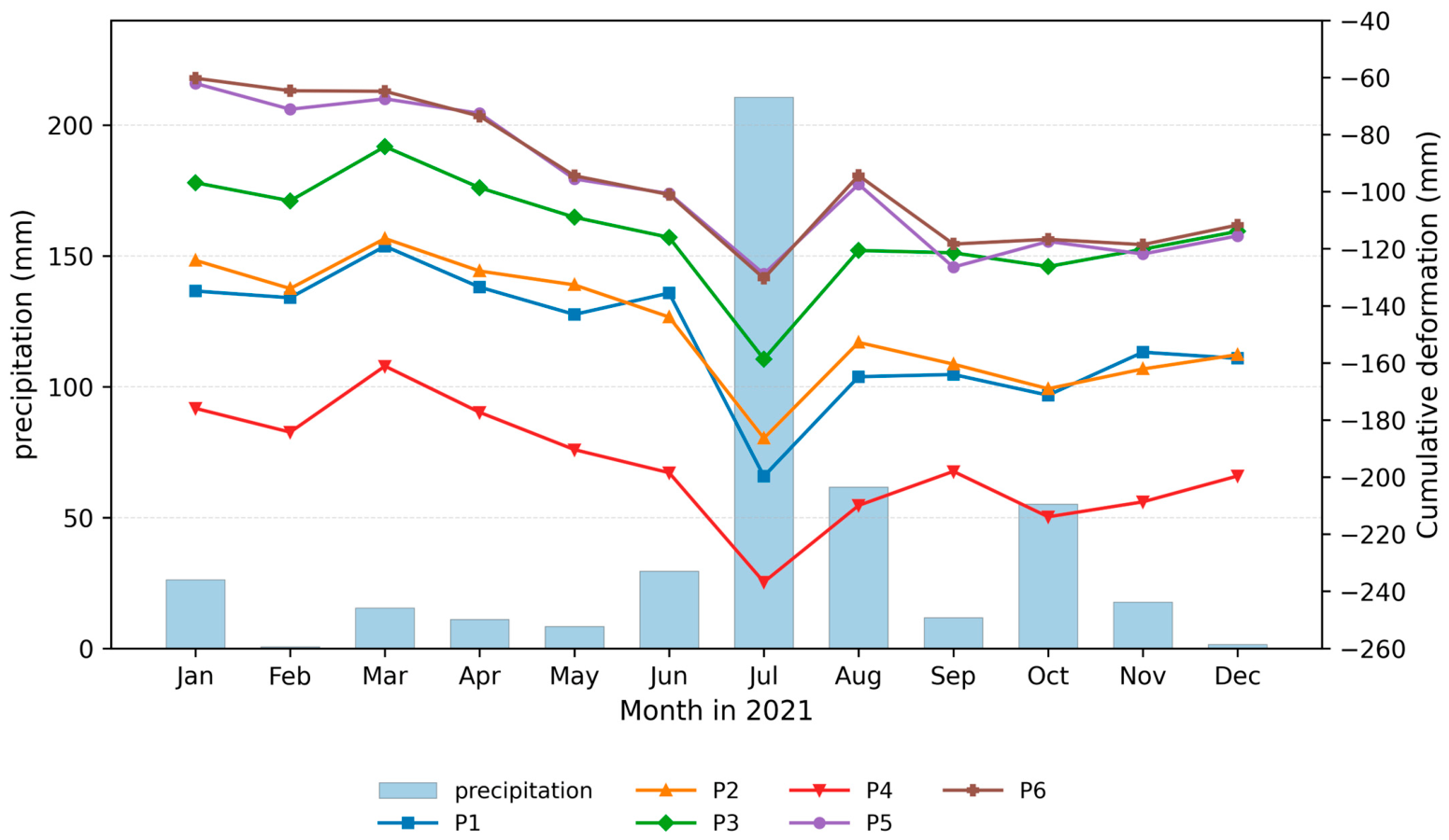
To further address the limitation that monthly rainfall subsidence analysis may not fully capture short term deformation responses induced by extreme rainfall, an event window comparison was conducted in the Zhengzhou sector of Study Area 3. Six representative coherent deformation points were selected from the subsiding areas, and their cumulative deformation was compared with monthly precipitation in 2021, with particular attention to the Henan “7.20” extreme rainfall event. The specific locations of the six points are shown in

Table 8. Geographic coordinates of the six representative deformation points in the Zhengzhou sector of Study Area 3.

Point	longitude (°E)	Latitude (°N)
P1	112.6838226	34.34162521
P2	112.6930084	34.34438705
P3	113.039711	34.33260727
P4	113.1891632	34.24527359
P5	113.0521698	34.32662964
P6	113.0540619	34.33272934

.

As shown in Figure 13, the precipitation in July 2021 reached its annual maximum, corresponding to the period of the 7.20 extreme rainfall event. During this month, all six points exhibited abrupt negative shifts in cumulative deformation, indicating that extreme rainfall can induce short term acceleration of subsidence.

However, the deformation response was not limited to rainfall induced subsidence acceleration. After the July rainfall peak, most points showed upward recovery or a clear reduction in subsidence rate from August onward, and the cumulative deformation curves became relatively stable in the following months. This pattern suggests a two stage hydromechanical response. During the rainfall peak, intense precipitation may increase surface water loading, promote rapid infiltration through mining-induced fractures and unconsolidated deposits, and weaken the overlying strata, thereby enhancing short term settlement. After the event, rainfall induced groundwater recharge may increase pore water pressure and reduce effective stress, causing partial rebound or a reduction in the subsequent subsidence rate.

The different response amplitudes among P1–P6 further indicate that the deformation response to extreme rainfall is spatially heterogeneous. Points located in more deformation sensitive zones showed stronger short term subsidence acceleration, whereas other points displayed weaker but still recognizable responses. This heterogeneity may be related to local mining disturbance, overburden structure, drainage conditions, and hydrogeological connectivity. Therefore, this event scale analysis complements the SHAP results by demonstrating that precipitation affects mining subsidence not only as a long-term explanatory factor but also as a short-term trigger of rapid deformation changes.

Because the multisource datasets used in this study have different spatial resolutions, resampling coarse resolution groundwater and precipitation data to the InSAR analytical grid may introduce smoothing effects and interpolation uncertainty. Therefore, the 1 km groundwater and precipitation variables should be interpreted as regional hydrological and meteorological background indicators rather than fine scale local controls at the InSAR pixel scale.

4.2. The Controlling Effect of Topographical Factors on Subsidence

The relationship between mining subsidence and topographical factors does not constitute a fixed correlation on a single scale; rather, it represents a complex relationship that changes with the spatial scope of the interaction. Although mining activities serve as the root cause of surface subsidence in mining areas, the results of the wavelet coherence analysis demonstrate that the spatial distribution and characteristics of surface deformation are largely controlled by the regional topographical background. This control effect does not represent simple linear causality; instead, it exhibits strong spatial scale differences and regional geomorphological heterogeneity. All four profile lines intersect the main subsidence areas of the mining regions; therefore, the wavelet results clearly reveal spatial orientation. The significant coherence regions are primarily distributed where the profile lines cross the main subsidence segments and the adjacent locations of these segments, whereas they generally remain weak in non-subsidence background segments. These findings indicate that the effects of topographical factors on subsidence feature obvious spatial selectivity. The multiscale coupling structure can be more easily identified only when the topographical background actually overlaps with the subsidence anomalies along the profile lines.

4.2.1. Influence of Regional Macroscopic Geomorphology on Subsidence Basins

The DEM, slope, and aspect display obvious differences in the wavelet coherence spectra, which suggests that the modes of action of these factors on the spatial patterns of subsidence are distinct. DEMs exhibit more stable medium scale and large-scale coherence in multiple study areas, particularly in Area 2 and Area 3. This finding indicates that the elevation background serves as a crucial foundation for the spatial differentiation of subsidence. However, elevation fluctuations do not directly drive the occurrence of subsidence; instead, they constitute the underlying geomorphological framework for the development of subsidence basins. Because the occurrence and exploitation of large-scale coal resources generally depend on specific geological structures and macroscale geomorphological environments, such as the edges of alluvial proluvial fans or the transition zones from low mountains and hills to plains, high-intensity continuous mining activities induce large-scale surface subsidence. This pattern indicates that broad mining-induced subsidence basins and regional elevation variations share similar spatial organization over relatively long distances. However, elevation does not directly initiate subsidence. The occurrence of coal resources, mining activities, overburden structures, geological units, and macroscale geomorphology may exhibit overlapping spatial distributions. Consequently, the large-scale coherence between elevation and subsidence may reflect the combined spatial organization of mining-induced deformation, geological conditions, and regional topography. It should therefore be interpreted as a regional-scale geomorphological association.

4.2.2. Spatial Influence of Local Topography on Surface Deformation Gradients

In contrast to the large-scale continuous constraints exhibited by elevation, the significant coherence areas between slope and subsidence across all four study areas manifested as local, small-scale discrete patches. This scaling characteristic suggests that the influence of slope magnitude on the spatial pattern of subsidence primarily occurs at the local micro level, where deformation is intense. Substantial differential deformation often occurs at the edges of mining subsidence troughs or at the intersection zones of multiple subsidence centers. In contrast to the relatively continuous medium- and large-scale coherence involving elevation, the significant coherence regions between slope or aspect and subsidence occur mainly as localized small-scale patches. These regions are concentrated primarily near the margins of subsidence troughs and at profile sections with relatively large deformation gradients. This spatial correspondence indicates that local terrain conditions are associated with the gradient and asymmetry of the observed deformation. From a geomorphological perspective, inclined terrain may increase the susceptibility of these locations to differential deformation, shear deformation, or local surface instability. However, these processes are physically plausible interpretations rather than mechanisms directly verified by WTC. Therefore, slope and aspect should be regarded as possible local modulation factors associated with the spatial expression of mining-induced deformation rather than as determinants of subsidence occurrence.

The profile results in Figure 8 and Figure 9 show the spatial locations and temporal evolution of representative subsidence sections, while the WTC results reveal the scale-dependent coherence between subsidence and topographic factors. These results indicate that the influence of topography on subsidence is not a simple linear causal relationship, but a multiscale modulation effect. At the regional scale, elevation and macroscale geomorphology provide the spatial framework for the development of broad subsidence basins. At the local scale, slope and aspect mainly modulate deformation intensity near the margins of subsidence troughs, where differential deformation gradients are more pronounced.

4.3. Implications for Mine Management and Ecological Restoration

The results of this study not only reveal the spatiotemporal evolution of subsidence and the relative explanatory contributions of the selected measurable variables of surface subsidence in the concentrated coal mining areas of Henan Province but also provide practical implications for mine safety management, groundwater regulation, land reclamation, and ecological restoration [63]. First, the SBAS-InSAR results derived from long-term Sentinel-1A observations indicate that subsidence in the study areas is characterized by strong spatial heterogeneity and continuous accumulation. Some subsidence centers remain relatively stable in location over multiple years, while their magnitudes and affected areas continue to expand [64]. Therefore, SBAS-InSAR can be incorporated into a routine dynamic monitoring system for mining areas, supporting full-process subsidence surveillance before, during, and after mining activities. Persistent subsidence centers, margins of subsidence troughs, areas above goafs, transportation corridors, village settlements, and industrial sites should be delineated as key risk control zones [65]. A hierarchical early warning system can be established by integrating the subsidence velocity, cumulative displacement, and deformation gradient. Regularly updated InSAR monitoring results would allow early identification and dynamic tracking of high-risk subsidence zones, thereby supporting safe mine production, engineering avoidance, infrastructure reinforcement, and geological hazard prevention [66].

Second, the XGBoost-SHAP results indicate that groundwater table depth represents the most important measurable explanatory factor within the selected variables for characterizing spatial differences in subsidence, while its model-based response pattern varies among different geological and geomorphological settings. In piedmont, low-mountain, and hilly mining areas, greater groundwater table depth may be associated with mine drainage and declining aquifer water levels. The resulting pore-pressure dissipation and effective-stress increase provide a possible mechanism through which groundwater disturbance may contribute to subsidence [67]. In contrast, the eastern plain area, shallow groundwater conditions, thick unconsolidated deposits, agricultural pumping, and mining disturbance may jointly contribute to soil compression and deformation. Therefore, groundwater management in mining areas should not follow a uniform strategy; instead, differentiated regulation should be implemented according to geological units [68]. For piedmont and hilly mining areas, mine drainage intensity should be carefully controlled, deep aquifer water levels should be continuously monitored, and the coupled relationships among water inrush control, mine drainage, and surface subsidence should be evaluated. For plain mining areas with thick unconsolidated layers, shallow groundwater exploitation should be regulated, and agricultural water use, mine drainage, and ecological water replenishment should be coordinated to avoid the aggravation of subsidence caused by abnormal groundwater fluctuations [69].

Finally, the WTC analysis identified scale-dependent spatial associations between topographic factors and subsidence patterns. Regional elevation showed relatively continuous associations with large-scale subsidence-basin patterns, whereas slope and aspect exhibited more localized associations near the margins of subsidence troughs and in zones with large deformation gradients. On the basis of this understanding, ecological restoration and land reclamation should not rely solely on the areal extent of subsidence but should comprehensively consider the subsidence intensity, deformation gradient, terrain slope, surface fracture risk, and land use type [70]. Areas located at the margins of subsidence troughs, steep slopes, zones with strong differential deformation, and regions prone to surface cracking should be prioritized for crack filling, slope stabilization, drainage system optimization, and vegetation restoration. With respect to low-lying waterlogged areas within subsidence basins, wetland restoration, water retention space construction, or farmland consolidation can be implemented according to local topographic conditions and land use demands [71]. In areas where subsidence has stabilized or where the subsidence rate has significantly decreased, land reclamation, ecological reconstruction, and construction land safety assessment can be gradually promoted. Overall, the integrated framework of SBAS-InSAR dynamic monitoring, XGBoost-SHAP driving-factor identification, and WTC-based multiscale topographic constraint analysis proposed in this study can provide scientific support for subsidence risk zoning, differentiated groundwater regulation, green-mining planning, and postmining ecological restoration [72].

4.4. Sensitivity Analysis of Potential Errors Caused by Horizontal Displacement During LOS to Vertical Projection

The conversion of LOS displacement to the vertical direction assumes that horizontal motion is negligible. To evaluate the uncertainty associated with this assumption, a sensitivity analysis was conducted using the actual incidence and LOS azimuth angles of the four study areas listed in Table 2. Five horizontal-to-vertical displacement ratios, namely 0.10, 0.20, 0.30, 0.44, and 0.50, were considered. For each ratio, the maximum absolute relative error was calculated by considering the most unfavorable horizontal-displacement direction. The effects of purely east–west and purely north–south displacement were also evaluated.

As shown in

Table 9. Sensitivity of the vertically projected displacement to horizontal motion under the imaging geometries of the four study areas.

Horizontal-to-Vertical Displacement Ratio (H/V)	Area 1 Maximum Error (%)	Area 2 Maximum Error (%)	Area 3 Maximum Error (%)	Area 4 Maximum Error (%)	East–West Error Range (%)	North–South Error Range (%)
0.10	7.49	6.76	8.34	7.12	6.64–8.21	1.25–1.46
0.20	14.99	13.52	16.68	14.25	13.29–16.42	2.51–2.93
0.30	22.48	20.28	25.01	21.37	19.93–24.63	3.76–4.39
0.44	32.97	29.75	36.69	31.34	29.23–36.12	5.51–6.44
0.50	37.47	33.80	41.69	35.61	33.22–41.04	6.26–7.32

, when the horizontal-to-vertical displacement ratio was 0.10, the maximum absolute errors ranged from 6.76% in Study Area 2 to 8.34% in Study Area 3. The corresponding ranges increased to 13.52–16.68% at a ratio of 0.20 and 20.28–25.01% at a ratio of 0.30. When the ratio reached 0.44 and 0.50, the maximum errors increased to 29.75–36.69% and 33.80–41.69%, respectively [73].

The differences among the four study areas were mainly related to their incidence angles because their satellite heading and LOS azimuth angles were relatively similar. Study Area 3, with the largest mean incidence angle of 39.82°, showed the highest sensitivity to horizontal displacement. In contrast, Study Area 2, with the smallest mean incidence angle of 34.06°, showed the lowest sensitivity [74]. The projection error also exhibited marked directional dependence. Across the five horizontal-to-vertical displacement ratios, the errors caused by east–west displacement were substantially larger than those caused by north–south displacement. At a ratio of 0.44, east–west displacement resulted in absolute errors of 29.23–36.12%, whereas the corresponding errors associated with north–south displacement were only 5.51–6.44%. This difference reflects the greater sensitivity of the Sentinel-1 ascending LOS geometry to east–west horizontal motion.

Horizontal displacement therefore has a relatively limited influence where vertical subsidence is strongly dominant. However, near the margins of mining-induced subsidence basins, where horizontal motion may become appreciable, the LOS-to-vertical conversion may substantially overestimate or underestimate vertical subsidence. This uncertainty is particularly relevant where the horizontal displacement contains a strong east–west component. The deformation values derived from the conversion are consequently interpreted as approximate vertically projected displacements rather than strictly decomposed vertical displacements.

4.5. Limitations

4.5.1. Limitations of XGBoost-SHAP Attribution and Spatial Validation

The original 70%/30% train–validation split was implemented at the random pixel level. Because neighboring observations in geospatial datasets are spatially autocorrelated, this strategy can produce optimistic estimates of model performance. To directly evaluate this effect, an additional fivefold spatial block cross-validation was conducted using 1 km spatial blocks. The spatial cross-validation R² values ranged from 0.626 to 0.841, which were lower than the random-validation values of 0.894–0.980, while the corresponding RMSE and MAE values increased. These differences confirm that spatial dependence contributed to the high performance obtained under random pixel-level validation [75].

Nevertheless, the positive spatial cross-validation R² values across all four study areas indicate that the models retained meaningful predictive capability when applied to spatially separated blocks. Therefore, the spatial cross-validation results support within-area spatial generalization at the tested scale but should not be interpreted as independent cross-regional transfer validation. The SHAP results are consequently interpreted as model-based associations and relative explanatory contributions within each study area rather than universally transferable causal relationships [76].

4.5.2. Limitations in Hydrogeological Data and Groundwater-Mechanism Verification

The interpretation of the groundwater–subsidence relationship is constrained by the lack of direct and spatially continuous hydrogeological observations at the provincial scale. Continuous mine drainage records, groundwater extraction rates, and site-specific aquifer parameters were unavailable. Therefore, the inferred groundwater influence and the response polarity reversal should be regarded as model-based response patterns derived from the groundwater table depth level grid dataset, SHAP results, and regional geological and hydrogeological settings, rather than as direct quantitative evidence of a complete hydrological mechanism. Future studies should integrate mine drainage records, groundwater extraction data, aquifer parameters, and in situ hydrological monitoring to further verify the groundwater–subsidence mechanism and the model-identified response polarity reversal.

4.5.3. Limitations in Urbanization and Mining Infrastructure Representation

Urbanization and mining infrastructure may also influence local subsidence heterogeneity. In this study, land-cover data and mining right boundaries were used as proxies for surface human activities and mining-related spatial constraints [77]. However, the single epoch CLCD 2020 dataset cannot fully capture temporal changes associated with mining expansion, industrial construction, subsidence pond development, land reclamation, and ecological restoration [78]. Consequently, the present analysis may smooth or underestimate the localized effects of urban construction and mining infrastructure on surface deformation. Future studies should incorporate high resolution built up area data, impervious surface products, nighttime light data, and time series information on mining infrastructure to better quantify the spatially heterogeneous effects of human activities on surface deformation [79].

5. Conclusions

On the basis of the SBAS-InSAR technique, this study conducted long-term monitoring of surface subsidence in concentrated coal mining areas of Henan Province using Sentinel-1A images from March 2017 to February 2025. Combined with XGBoost-SHAP and wavelet coherence analysis, the relative explanatory contributions of selected measurable environmental and topographic variables were investigated within mining-affected areas from both temporal and spatial perspectives. The research findings are as follows:

(1)

Surface subsidence in Henan Province’s coal mining areas is characterized by significant spatial heterogeneity and continuous accumulation. High-subsidence zones primarily occur in concentrated coal development regions and align well with mining boundaries and extraction ranges. From 2017 to 2025, the subsidence center locations across the study area generally remain stable, whereas the subsidence amplitude continuously increases and the range of influence expands, eventually leading to the formation of continuous subsidence troughs. Study Area 3 experiences the most intense subsidence, reaching a maximum cumulative value of −2101 mm, indicating a significant impact from long-term mining disturbances. A local validation conducted within a representative mining area in Study Area 3 showed good agreement between the SBAS-InSAR-derived and leveling-derived displacements at 14 benchmarks during the period from 5 May to 20 July 2023, with an R² of 0.816 and an RMSE of 9.22 mm.

(2)

The mining-rights boundaries and the temporal correspondence between documented mining commencement and the subsequent development of persistent subsidence support underground mining as the fundamental physical forcing of the observed deformation. However, detailed mining-intensity parameters were not available for inclusion in the XGBoost-SHAP models. Accordingly, the SHAP analysis characterizes the conditional explanatory and modulating roles of the selected environmental and topographic variables in the spatial heterogeneity of mining-induced subsidence, rather than quantifying the contribution of mining activity itself. Among the selected variables included in the models, groundwater table depth represents the most important measurable explanatory factor, although its effect direction varied with geological and hydrogeological setting.

(3)

Wavelet coherence analysis identified scale-dependent spatial associations between subsidence and topographic factors along the representative profiles. The significant coherence regions were concentrated mainly in profile segments crossing the principal subsidence zones, and their continuity varied with the spatial continuity of the subsidence belts. Elevation exhibited relatively continuous medium- and large-scale associations with broad subsidence-basin patterns, particularly in Areas 2 and 3, whereas slope and aspect showed more localized small-scale associations near subsidence-trough margins and sections with large deformation gradients. These results characterize multiscale spatial correspondence between topography and mining-induced deformation.

(4)

Mining activities constitute the fundamental physical cause of surface subsidence, while multisource environmental and topographic variables help characterize the spatial differentiation of deformation within mining-affected areas. Temporal comparisons confirm that accelerated subsidence evolution at monitoring points corresponds closely to mining activity cycles. Given the difficulty of directly acquiring refined cross-regional underground mining parameters, this study reveals that large-scale quantifiable variables, such as groundwater, precipitation, and topography, can be used to explain and compare spatial variations in deformation responses across different geological units, but these variables should not be interpreted as replacing mining activity as the primary cause of subsidence.

In summary, beyond the application of established methods, the main contribution of this study lies in establishing a consistent province-scale comparative framework for four coal-mining regions with contrasting geological, geomorphological, and hydrogeological backgrounds. Henan Province provides a valuable natural regional comparison setting because piedmont, mountainous, transitional, and thick alluvial-sediment mining environments coexist within the same province. The comparative results show that groundwater table depth exhibits regionally contrasting model-based response patterns, while topographic variables display scale-dependent spatial associations with subsidence morphology.

The results also have practical implications for mine management and ecological restoration. Long-term SBAS-InSAR observations can support the identification of persistent subsidence centers, subsidence-basin margins, and zones with large deformation gradients, thereby providing information for geological-hazard zoning, infrastructure protection, and reinforcement planning. The regional differences revealed by the XGBoost-SHAP analysis may assist groundwater management and mine-drainage zoning, while the multiscale spatial relationships identified by the wavelet analysis can support the delineation of ecological-restoration priorities, post-mining land reclamation, and green-mining planning.

References

1. Ren, S.-H.; Jiao, X.-M.; Zheng, D.-Z.; Zhang, Y.-N.; Xie, H.-P.; Guo, Z.-Q. Demand and Fluctuation Range of China’s Coal Production under the Dual Carbon Target. Energy Rep. 2024, 11, 3267–3282. [Google Scholar] [CrossRef] [Scilit]
2. Li, J.; Tan, Z.; Zeng, N.; Xu, L.; Yang, Y.; Siddique, A.; Dang, J.; Zhang, J.; Wang, X. Wavelet-Based Analysis of Subsidence Patterns and High-Risk Zone Delineation in Underground Metal Mining Areas Using Sbas-Insar. Land 2025, 14, 992. [Google Scholar] [CrossRef] [Scilit]
3. Tataru, A.C.; Tataru, D.; Popescu, F.D.; Andras, A.; Brinas, I. Simulation of Land Subsidence Caused by Coal Mining at the Lupeni Mining Exploitation Using Comsol Multiphysics. Appl. Sci. 2025, 15, 10651. [Google Scholar] [CrossRef] [Scilit]
4. Karanam, V.; Motagh, M.; Garg, S.; Jain, K. Multi-Sensor Remote Sensing Analysis of Coal Fire Induced Land Subsidence in Jharia Coalfields, Jharkhand, India. Int. J. Appl. Earth Obs. Geoinf. 2021, 102, 102439. [Google Scholar] [CrossRef] [Scilit]
5. Zhang, K.; Zhao, Y.; Confuorto, P.; Moretti, S.; Fibbi, G.; Ling, C.; Xu, D.; Guo, J.; Zhao, L. Ground Residual Subsidence During Post-Mining Period Based on Sentinel-1 and Ps-Insar Technology: The Shendong Coal Field (China) Case Study. Geomech. Geophys. Geo-Energy Geo-Resour. 2025, 12, 30. [Google Scholar] [CrossRef] [Scilit]
6. Kang, S.; Jia, X.; Zhao, Y.; Ao, Y.; Ma, C. Spatiotemporal Relationship between Land Subsidence and Ecological Environmental Quality in Shenfu Mining Area, Loess Plateau, China. ISPRS Int. J. Geo-Inf. 2024, 13, 390. [Google Scholar] [CrossRef] [Scilit]
7. Aobpaet, A.; Caro Cuenca, M.; Hooper, A.; Trisirisatayawong, I. Insar Time-Series Analysis of Land Subsidence in Bangkok, Thailand. Int. J. Remote Sens. 2013, 34, 2969–2982. [Google Scholar] [CrossRef] [Scilit]
8. Gojković, Z.; Kilibarda, M.; Brajović, L.; Marjanović, M.; Milutinović, A.; Ganić, A. Ground Surface Subsidence Monitoring Using Sentinel-1 in the “Kostolac” Open Pit Coal Mine. Remote Sens. 2023, 15, 2519. [Google Scholar] [CrossRef] [Scilit]
9. Ferretti, A.; Prati, C.; Rocca, F. Permanent Scatterers in Sar Interferometry. IEEE Trans. Geosci. Remote Sens. 2001, 39, 8–20. [Google Scholar] [CrossRef] [Scilit]
10. Tian, Z.; Zhao, L.; Fan, H.; Lin, T.; Li, T. Mining Subsidence Monitoring Using Distributed Scatterers Insar Based on Goldstein Filter and Fisher Information Matrix-Weighted Optimization. Nat. Hazards 2024, 120, 4205–4231. [Google Scholar] [CrossRef] [Scilit]
11. Ma, Z.; Yang, X.; Xie, L.; Dong, W. Life Cycle Mining Deformation Monitoring and Analysis Using Sentinel-1 and Radarsat-2 Insar Time Series. Remote Sens. 2024, 16, 2335. [Google Scholar] [CrossRef] [Scilit]
12. Maghsoudi, Y.; van der Meer, F.; Hecker, C.; Perissin, D.; Saepuloh, A. Using Ps-Insar to Detect Surface Deformation in Geothermal Areas of West Java in Indonesia. Int. J. Appl. Earth Obs. Geoinf. 2018, 64, 386–396. [Google Scholar] [CrossRef] [Scilit]
13. Li, S.; Xu, W.; Li, Z. Review of the Sbas Insar Time-Series Algorithms, Applications, and Challenges. Geod. Geodyn. 2022, 13, 114–126. [Google Scholar] [CrossRef] [Scilit]
14. Bai, Z.; Zhao, F.; Wang, J.; Li, J.; Wang, Y.; Li, Y.; Lin, Y.; Shen, W. Revealing Long-Term Displacement and Evolution of Open-Pit Coal Mines Using Sbas-Insar and Ds-Insar. Remote Sens. 2025, 17, 1821. [Google Scholar] [CrossRef] [Scilit]
15. Bischoff, C.A.; Ferretti, A.; Novali, F.; Uttini, A.; Giannico, C.; Meloni, F. Nationwide Deformation Monitoring with Squeesar® Using Sentinel-1 Data. Proc. Int. Assoc. Hydrol. Sci. 2020, 382, 31–37. [Google Scholar] [CrossRef] [Scilit]
16. Liu, Y.; Yang, H.; Wang, S.; Xu, L.; Peng, J. Monitoring and Stability Analysis of the Deformation in the Woda Landslide Area in Tibet, China by the Ds-Insar Method. Remote Sens. 2022, 14, 532. [Google Scholar] [CrossRef] [Scilit]
17. Gu, X.; Li, Y.; Zuo, X.; Bu, J.; Yang, F.; Yang, X.; Li, Y.; Zhang, J.; Huang, C.; Shi, C. Image Compression–Based Ds-Insar Method for Landslide Identification and Monitoring of Alpine Canyon Region: A Case Study of Ahai Reservoir Area in Jinsha River Basin. Landslides 2024, 21, 2501. [Google Scholar] [CrossRef] [Scilit]
18. Feng, W.; Dun, J.; Yi, X.; Zhang, G. Deformation Analysis of Woda Village Old Landslide in Jinsha River Basin Using Sbas-Insar Technology. J. Eng. Geol. 2020, 28, 384–393. [Google Scholar]
19. Su, X.; Zhang, Y.; Meng, X.; Ur Rehman, M.; Yue, D.; Zhao, Y.; Zhou, Z.; Guo, F.; Zhou, Q.; Niu, B. An Integrated Landslide Susceptibility Assessment in the Karakoram Mountains Based on Sbas-Insar and Machine Learning: A Case Study of the Hunza Valley. Bull. Eng. Geol. Environ. 2025, 84, 280. [Google Scholar] [CrossRef] [Scilit]
20. Berardino, P.; Fornaro, G.; Lanari, R.; Sansosti, E. A New Algorithm for Surface Deformation Monitoring Based on Small Baseline Differential Sar Interferograms. IEEE Trans. Geosci. Remote Sens. 2003, 40, 2375–2383. [Google Scholar]
21. Lanari, R.; Casu, F.; Manzo, M.; Zeni, G.; Berardino, P.; Manunta, M.; Pepe, A. An Overview of the Small Baseline Subset Algorithm: A Dinsar Technique for Surface Deformation Analysis. Pure Appl. Geophys. 2007, 164, 637–661. [Google Scholar] [CrossRef] [Scilit]
22. Jiang, X.; Shi, W.; Liang, F.; Gui, J.; Li, J. Insar-Derived Surface Deformation Characteristics and Mining Subsidence Parameters in Mountain Coal Mines. J. Mt. Sci. 2024, 21, 3139–3156. [Google Scholar] [CrossRef] [Scilit]
23. Wang, Y.; Cui, X.; Ge, C.; Che, Y.; Zhao, Y.; Li, P.; Jiang, Y.; Han, X. Monitoring Nonlinear Large Gradient Subsidence in Mining Areas through Sbas-Insar with Punet and Weibull Model Fusion. Environ. Sci. Pollut. Res. 2024, 31, 52815–52826. [Google Scholar] [CrossRef] [Scilit] [PubMed]
24. Tizzani, P.; Berardino, P.; Casu, F.; Euillades, P.; Manzo, M.; Ricciardi, G.P.; Zeni, G.; Lanari, R. Surface Deformation of Long Valley Caldera and Mono Basin, California, Investigated with the Sbas-Insar Approach. Remote Sens. Environ. 2007, 108, 277–289. [Google Scholar] [CrossRef] [Scilit]
25. Głąbicki, D. Displacement Time Series Forecasting Using Sentinel-1 Sbas-Insar Results in a Mining Subsidence Case Study—Evaluation of Machine Learning and Deep Learning Methods. Remote Sens. 2025, 17, 3905. [Google Scholar] [CrossRef] [Scilit]
26. Riyas, M.J.; Syed, T.H.; Kumar, H.; Kuenzer, C. Detecting and Analyzing the Evolution of Subsidence Due to Coal Fires in Jharia Coalfield, India Using Sentinel-1 Sar Data. Remote Sens. 2021, 13, 1521. [Google Scholar] [CrossRef] [Scilit]
27. Zhang, Z.; Li, Y.; Gao, S. Surface Deformation Monitoring and Spatiotemporal Evolution Analysis of Open-Pit Mines Using Small-Baseline Subset and Distributed-Scatterer Insar to Support Sustainable Mine Operations. Sustainability 2025, 17, 8834. [Google Scholar] [CrossRef] [Scilit]
28. Xu, Y.; Li, T.; Tang, X.; Zhang, X.; Fan, H.; Wang, Y. Research on the Applicability of Dinsar, Stacking-Insar and Sbas-Insar for Mining Region Subsidence Detection in the Datong Coalfield. Remote Sens. 2022, 14, 3314. [Google Scholar] [CrossRef] [Scilit]
29. Zhou, Z.; Hu, J.; Wang, J.; Wang, L.; Qiao, T.; Li, Z.; Cheng, S. Identifying Spatiotemporal Pattern and Trend Prediction of Land Subsidence in Zhengzhou Combining Mt-Insar, Xgboost and Hydrogeological Analysis. Sci. Rep. 2025, 15, 3848. [Google Scholar] [CrossRef] [Scilit] [PubMed]
30. Wang, Y.; Gong, H.; Zhou, C.; Wang, Q.; Wang, H.; Zhang, J. Decomposition and Attribution Analysis of the Coupled Evolution Characteristics of Groundwater and Land Subsidence in the Beijing-Tianjin-Hebei Plain. J. Hydrol. Reg. Stud. 2025, 59, 102393. [Google Scholar] [CrossRef] [Scilit]
31. Yang, G.; McCoy, K. Modeling Groundwater-Level Responses to Multiple Stresses Using Transfer-Function Models and Wavelet Analysis in a Coastal Aquifer System. J. Hydrol. 2023, 627, 130426. [Google Scholar] [CrossRef] [Scilit]
32. Gu, X.; Sun, H.; Zhang, Y.; Zhang, S.; Lu, C. Partial Wavelet Coherence to Evaluate Scale-Dependent Relationships between Precipitation/Surface Water and Groundwater Levels in a Groundwater System. Water Resour. Manag. 2022, 36, 2509–2522. [Google Scholar] [CrossRef] [Scilit]
33. Hu, W.; Si, B. Improved Partial Wavelet Coherency for Understanding Scale-Specific and Localized Bivariate Relationships in Geosciences. Hydrol. Earth Syst. Sci. 2021, 25, 321–331. [Google Scholar] [CrossRef] [Scilit]
34. Zhang, J.; Gao, J.; Gao, F. Time Series Land Subsidence Monitoring and Prediction Based on Sbas-Insar and Geotemporal Transformer Model. Earth Sci. Inform. 2024, 17, 5899–5911. [Google Scholar] [CrossRef] [Scilit]
35. Belgiu, M.; Drăguţ, L. Random Forest in Remote Sensing: A Review of Applications and Future Directions. ISPRS J. Photogramm. Remote Sens. 2016, 114, 24–31. [Google Scholar] [CrossRef] [Scilit]
36. Li, F.; Liu, G.; Tao, Q.; Zhai, M. Land Subsidence Prediction Model Based on Its Influencing Factors and Machine Learning Methods. Nat. Hazards 2023, 116, 3015–3041. [Google Scholar]
37. Niazkar, M.; Menapace, A.; Brentan, B.; Piraei, R.; Jimenez, D.; Dhawan, P.; Righetti, M. Applications of Xgboost in Water Resources Engineering: A Systematic Literature Review (Dec 2018–May 2023). Environ. Model. Softw. 2024, 174, 105971. [Google Scholar] [CrossRef] [Scilit]
38. Zhang, J.; Ma, X.; Zhang, J.; Sun, D.; Zhou, X.; Mi, C.; Wen, H. Insights into Geospatial Heterogeneity of Landslide Susceptibility Based on the Shap-Xgboost Model. J. Environ. Manag. 2023, 332, 117357. [Google Scholar] [CrossRef] [Scilit] [PubMed]
39. Quoc, H.N.D.; Trong, N.G.; Khien, H.T.; Duc Tinh, L.; Van Anh, T. Machine Learning Approaches for Predicting Land Subsidence in Ca Mau: XGBoost, Random Forest, and MAF. J. Pol. Mineral. Eng. Soc. 2025, 1, 703. [Google Scholar] [CrossRef] [Scilit]
40. Seihani, R.; Gholami, H.; Esmaeilpour, Y.; Kamali, A.; Zareh, M. Interpretation Techniques to Explain the Output of a Spatial Land Subsidence Hazard Model in an Area with a Diverted Tributary. Appl. Comput. Geosci. 2024, 23, 100191. [Google Scholar] [CrossRef] [Scilit]
41. Xu, T.; Su, H.; Xiong, X.; Wang, W.; Dewan, A. Optimization of Land Subsidence Prediction Features Using Machine Learning and Shap Analysis with Sentinel-1 Insar Data in Chengdu and Chongqing, China. Geocarto Int. 2026, 41, 2617682. [Google Scholar] [CrossRef] [Scilit]
42. Kruk, M. Shap-Net, a Network Based on Shapley Values as a New Tool to Improve the Explainability of the Xgboost-Shap Model for the Problem of Water Quality. Environ. Model. Softw. 2025, 188, 106403. [Google Scholar] [CrossRef] [Scilit]
43. Lv, J.; Zhang, R.; Shama, A.; Hong, R.; He, X.; Wu, R.; Bao, X.; Liu, G. Exploring the Spatial Patterns of Landslide Susceptibility Assessment Using Interpretable Shapley Method: Mechanisms of Landslide Formation in the Sichuan-Tibet Region. J. Environ. Manag. 2024, 366, 121921. [Google Scholar] [CrossRef] [Scilit] [PubMed]
44. Yu, B.; Xing, H.; Ge, W.; Yan, J.; Li, Y.-A. Explainable Machine Learning-Based Land Subsidence Susceptibility Mapping: From Feature Importance to Individual Model Contributions in Ensembled System. Earth Sci. Inform. 2025, 18, 407. [Google Scholar] [CrossRef] [Scilit]
45. Deng, H.; Li, L.; Yang, W. Quantifying Multifactorial Effects on Land Subsidence Using Interpretable Machine Learning: A Case Study in Cangzhou, China. Appl. Spat. Anal. Policy 2025, 18, 139. [Google Scholar] [CrossRef] [Scilit]
46. Shahnazi, S.; Roushangar, K.; Khodaei, B.; Hashemi, H. Insights into the Interconnected Dynamics of Groundwater Drought and Insar-Derived Subsidence in the Marand Plain, Northwestern Iran. Remote Sens. 2025, 17, 1173. [Google Scholar] [CrossRef] [Scilit]
47. Jiao, S.; Li, X.; Yu, J.; Lyu, M.; Zhang, K.; Li, Y.; Shi, P. Multi-Scale Analysis of Surface Building Density and Land Subsidence Using a Combination of Wavelet Transform and Spatial Autocorrelation in the Plains of Beijing. Sustainability 2024, 16, 2801. [Google Scholar] [CrossRef] [Scilit]
48. Zhang, H.; Rui, X.; Zhou, Y.; Sun, W.; Xie, W.; Gao, C.; Ren, Y. Analysis of the Response of Shallow Groundwater Levels to Precipitation Based on Different Wavelet Scales—A Case Study of the Datong Basin, Shanxi. Water 2024, 16, 2920. [Google Scholar] [CrossRef] [Scilit]
49. Zhu, M.; Yu, X.; Tan, H.; Yuan, J.; Chen, K.; Xie, S.; Han, Y.; Long, W. High-Precision Monitoring and Prediction of Mining Area Surface Subsidence Using Sbas-Insar and Cnn-Bigru-Attention Model. Sci. Rep. 2024, 14, 28968. [Google Scholar] [CrossRef] [Scilit] [PubMed]
50. Gao, M.; Gong, H.; Chen, B.; Li, X.; Zhou, C.; Shi, M.; Si, Y.; Chen, Z.; Duan, G. Regional Land Subsidence Analysis in Eastern Beijing Plain by Insar Time Series and Wavelet Transforms. Remote Sens. 2018, 10, 365. [Google Scholar] [CrossRef] [Scilit]
51. Snoeij, P.; Attema, E.; Davidson, M.; Duesmann, B.; Floury, N.; Levrini, G.; Rommen, B.; Rosich, B. The Sentinel-1 Radar Mission: Status and Performance. In Proceedings of the 2009 International Radar Conference “Surveillance for a Safer World” (RADAR 2009), Bordeaux, France, 12–16 October 2009. [Google Scholar]
52. Wang, M.; Yao, J.; Chang, H.; Liu, R.; Cao, Y.; Zhao, Y. Monthly Groundwater Level Grid Dataset of China Region (2005–2022); National Tibetan Plateau Data Center: Beijing, China, 2025. [Google Scholar]
53. Wang, M.; Yao, J.; Chang, H.; Liu, R.; Xu, N.; Liu, Z.; Gong, H.; Zheng, H.; Wang, J.; Guo, X. Underground Well Water Level Observation Grid Dataset from 2005 to 2022. Sci. Data 2025, 12, 728. [Google Scholar] [CrossRef] [Scilit] [PubMed]
54. Xu, J.; Yan, C.; Waseem Boota, M.; Chen, X.; Li, Z.; Liu, W.; Yan, X. Research on Automatic Identification of Coal Mining Subsidence Area Based on Insar and Time Series Classification. J. Clean. Prod. 2024, 470, 143293. [Google Scholar] [CrossRef] [Scilit]
55. Liu, Y.; Yan, X.; Xia, Y.; Liu, B.; Lu, Z.; Yu, M. Characterizing Spatiotemporal Patterns of Land Subsidence after the South-to-North Water Diversion Project Based on Sentinel-1 Insar Observations in the Eastern Beijing Plain. Remote Sens. 2022, 14, 5810. [Google Scholar] [CrossRef] [Scilit]
56. Navarro-Hernández, M.I.; Valdes-Abellan, J.; Tomás, R.; Lopez-Sanchez, J.M.; Ezquerro, P.; Bru, G.; Bonì, R.; Meisina, C.; Herrera, G. Valinsar: A Systematic Approach for the Validation of Differential Sar Interferometry in Land Subsidence Areas. IEEE J. Sel. Top. Appl. Earth Obs. Remote Sens. 2022, 15, 3650–3671. [Google Scholar] [CrossRef] [Scilit]
57. Pham, B.T.; Shirzadi, A.; Bui, D.T.; Prakash, I.; Dholakia, M. A Hybrid Machine Learning Ensemble Approach Based on a Radial Basis Function Neural Network and Rotation Forest for Landslide Susceptibility Modeling: A Case Study in the Himalayan Area, India. Int. J. Sediment Res. 2018, 33, 157–170. [Google Scholar] [CrossRef] [Scilit]
58. Peng, J.; Qiao, R.; Liu, Y.; Blaschke, T.; Li, S.; Wu, J.; Xu, Z.; Liu, Q. A Wavelet Coherence Approach to Prioritizing Influencing Factors of Land Surface Temperature and Associated Research Scales. Remote Sens. Environ. 2020, 246, 111866. [Google Scholar] [CrossRef] [Scilit]
59. Martínez, B.; Gilabert, M.A. Vegetation Dynamics from Ndvi Time Series Analysis Using the Wavelet Transform. Remote Sens. Environ. 2009, 113, 1823–1842. [Google Scholar] [CrossRef] [Scilit]
60. McFeeters, S.K. The Use of the Normalized Difference Water Index (Ndwi) in the Delineation of Open Water Features. Int. J. Remote Sens. 1996, 17, 1425–1432. [Google Scholar] [CrossRef] [Scilit]
61. Oke, T.R. The Energetic Basis of the Urban Heat Island. Q. J. R. Meteorol. Soc. 1982, 108, 1–24. [Google Scholar] [CrossRef] [Scilit]
62. Tomás, R.; Li, Z.; Lopez-Sanchez, J.M.; Liu, P.; Singleton, A. Using Wavelet Tools to Analyse Seasonal Variations from Insar Time-Series Data: A Case Study of the Huangtupo Landslide. Landslides 2016, 13, 437–450. [Google Scholar] [CrossRef] [Scilit]
63. Chen, Z.; Yang, Y.; Zhou, L.; Hou, H.; Zhang, Y.; Liang, J.; Zhang, S. Ecological Restoration in Mining Areas in the Context of the Belt and Road Initiative: Capability and Challenges. Environ. Impact Assess. Rev. 2022, 95, 106767. [Google Scholar] [CrossRef] [Scilit]
64. Xu, H.; Xu, F.; Lin, T.; Xu, Q.; Yu, P.; Wang, C.; Aili, A.; Zhao, X.; Zhao, W.; Zhang, P. A Systematic Review and Comprehensive Analysis on Ecological Restoration of Mining Areas in the Arid Region of China: Challenge, Capability and Reconsideration. Ecol. Indic. 2023, 154, 110630. [Google Scholar] [CrossRef] [Scilit]
65. Xiang, Y.; Gong, J.; Zhang, L.; Zhang, M.; Chen, J.; Liang, H.; Chen, Y.; Fu, X.; Su, R.; Luo, Y. Research Progress of Mine Ecological Restoration Technology. Resources 2025, 14, 100. [Google Scholar] [CrossRef] [Scilit]
66. Young, R.E.; Gann, G.D.; Walder, B.; Liu, J.; Cui, W.; Newton, V.; Nelson, C.R.; Tashe, N.; Jasper, D.; Silveira, F.A. International Principles and Standards for the Ecological Restoration and Recovery of Mine Sites. Restor. Ecol. 2022, 30, e13771. [Google Scholar] [CrossRef] [Scilit]
67. Zhao, L.; Ren, T.; Wang, N. Groundwater Impact of Open Cut Coal Mine and an Assessment Methodology: A Case Study in Nsw. Int. J. Min. Sci. Technol. 2017, 27, 861–866. [Google Scholar] [CrossRef] [Scilit]
68. Raghavendra, N.S.; Deka, P.C. Sustainable Development and Management of Groundwater Resources in Mining Affected Areas: A Review. Procedia Earth Planet. Sci. 2015, 11, 598–604. [Google Scholar] [CrossRef] [Scilit]
69. Thomann, J.A.; Werner, A.D.; Irvine, D.J.; Currell, M.J. Adaptive Management in Groundwater Planning and Development: A Review of Theory and Applications. J. Hydrol. 2020, 586, 124871. [Google Scholar] [CrossRef] [Scilit]
70. Huang, G.; Dong, J.; Xi, W.; Zhao, Z.; Li, S.; Kuang, Z.; An, Q.; Wei, J.; Zhu, Y. Study on Surface Deformation Pattern in Mine Closure Area of Complex Karst Mountainous Region Based on Sbas-Insar Technology. Front. Earth Sci. 2024, 11, 1353593. [Google Scholar] [CrossRef] [Scilit]
71. Meng, Z.; Wang, Y.; Tian, Y. Advances in Key Technologies for the Management, Restoration, Development, and Utilization of Coal Mining Subsidence Areas. Coal Geol. Explor. 2025, 53, 21. [Google Scholar]
72. Mao, Z.; Wang, M.; Chu, J.; Sun, J.; Liang, W.; Yu, H. Feature Extraction and Analysis of Reclaimed Vegetation in Ecological Restoration Area of Abandoned Mines Based on Hyperspectral Remote Sensing Images. J. Arid Land 2024, 16, 1409–1425. [Google Scholar] [CrossRef] [Scilit]
73. Yang, Z.; Li, Z.; Zhu, J.; Wang, Y.; Wu, L. Use of Sar/Insar in Mining Deformation Monitoring, Parameter Inversion, and Forward Predictions: A Review. IEEE Geosci. Remote Sens. Mag. 2020, 8, 71–90. [Google Scholar] [CrossRef] [Scilit]
74. Fikri, S.; Anjasmara, I.M.; Cahyadi, M.N.; Maulida, P. Impact of Multi–Source Dem Accuracy on Integrated Insar Time–Series Processing for 3d Deformation Decomposition in the Pasuruan Fault Zone. Earth Sci. Inform. 2026, 19, 114. [Google Scholar] [CrossRef] [Scilit]
75. Qu, L.; Hai, R.; Liang, K.; Zheng, Q.; Jin, M. Multi-Scale Attribution of Land Surface Temperature Driving Mechanisms in a Cold Region City: A Study on Spatial Non-Stationarity and Nonlinearity Based on Xgboost-Shap. Sustainability 2026, 18, 4451. [Google Scholar] [CrossRef] [Scilit]
76. Song, Y.; Cao, X.; Wang, H.; Zhang, B.; Zeng, H.; Liang, Y. Explaining Spatially Heterogeneous Drivers of Urban Expansion with an Xgboost–Shap–Ugm Framework. GIScience Remote Sens. 2026, 63, 2652154. [Google Scholar] [CrossRef] [Scilit]
77. Jara, Á.M.; Cofré, D.S.; Mansilla-Quiñones, P.; Mena, J.P.; Carvajal, M.-S.C. Socio-Ecological Controversies between Desalination, Urbanization, and Green Mining Transition. Extr. Ind. Soc. 2026, 26, 101866. [Google Scholar] [CrossRef] [Scilit]
78. Wirth, P.; Chang, J.; Syrbe, R.-U.; Wende, W.; Hu, T. Green Infrastructure: A Planning Concept for the Urban Transformation of Former Coal-Mining Cities. Int. J. Coal Sci. Technol. 2018, 5, 78–91. [Google Scholar] [CrossRef] [Scilit]
79. Pereira, A.C. Mining, Cities, and Development: A Critical Review of Socioeconomic, Environmental, and Spatial Transformations. Ciênc. Exatas Terra 2025, 29, 152. [Google Scholar] [CrossRef] [Scilit]
Figure 1. Locations of the study areas and leveling benchmarks. (a) Spatial distribution of the four mining study areas in Henan Province and the coverage of the Sentinel-1 imagery. (b) Location of Study Area 3 and the representative mining area used for local validation. (c) Spatial distribution of the 14 leveling benchmarks within the representative mining area. The terrain image in panel (c) was obtained from Google Maps (https://maps.google.com, accessed on 15 February 2025).
Remotesensing 18 02711 g001
Figure 2. Methodological workflow for surface subsidence monitoring and driving factor analysis.
Remotesensing 18 02711 g002
Figure 3. Spatiotemporal baseline networks of Sentinel-1A interferograms used for SBAS-InSAR processing in the study areas: (a) Area 1; (b) Area 2; (c) Area 3; and (d) Area 4.
Remotesensing 18 02711 g003
Figure 4. Verification of surface subsidence rates (2017–2025) and accuracy in coal mining areas of Henan Province (a) Overall spatial distribution of subsidence rates across the province. (b) Detailed map of subsidence rates in Study Area 1. (c) Detailed map of subsidence rates in Study Area 4. (d) Detailed map of subsidence rates in Study Area 2. (e) Detailed map of subsidence rates in Study Area 3. (f) Comparison between the SBAS-InSAR-derived vertically projected displacements and leveling-derived vertical displacements at 14 benchmarks within a representative mining area in Study Area 3 from 5 May to 20 July 2023. Different color bar ranges are used for the subpanels to preserve local deformation details within each study area because the deformation magnitude differs substantially among the four areas. Cross-area comparisons should therefore be based on the annotated deformation values and statistical results rather than on color tones alone.
Remotesensing 18 02711 g004
Figure 5. Comparison of leveling-derived vertical displacements and SBAS-InSAR-derived vertically projected displacements at 14 benchmarks within a representative mining area in Study Area 3 from 5 May to 20 July 2023.
Remotesensing 18 02711 g005
Figure 6. SBAS-InSAR time series (2017–2024). (a) Cumulative subsidence maps for Study Area 1. (b) Cumulative subsidence maps for Study Area 2. (c) Cumulative subsidence maps for Study Area 3. (d) Cumulative subsidence maps for the Study Area 4.
Remotesensing 18 02711 g006
Figure 7. Temporal correspondence between cumulative subsidence and mining activities at typical monitoring points (the subplots display the cumulative subsidence time series for selected monitoring points, with red dashed lines indicating the onset of the effective mining periods).
Remotesensing 18 02711 g007
Figure 8. Spatial distribution of typical profile lines traversing primary subsidence troughs. (a) Location of the profile line in Study Area 1. (b) Location of the profile line in Study Area 2. (c) Location of the profile line in Study Area 3. (d) Location of the profile line in Study Area 4. All the profile lines are oriented from point a to point b.
Remotesensing 18 02711 g008
Figure 9. Temporal evolution results of cumulative subsidence along representative profile lines (2017–2024). (a) Profile curve of Study Area 1. (b) Profile curve of Study Area 2. (c) Profile curve of Study Area 3. (d) Profile curve of Study Area 4. Local minor fluctuations in the profiles should be interpreted with reference to the RMSE of 9.22 mm obtained from validation against leveling measurements.
Remotesensing 18 02711 g009
Figure 10. SHAP analysis of the relative contributions and model-based response patterns of the explanatory variables associated with surface subsidence. (a) Contribution ranking and SHAP value scatter plot of Study Area 1. (b) Contribution ranking and SHAP value scatter plot of Study Area 2. (c) Contribution ranking and SHAP value scatter plot of Study Area 3. (d) Contribution ranking and SHAP value scatter plot of Study Area 4.
Remotesensing 18 02711 g010
Figure 11. Association matrices of the explanatory variables in the four study areas.
Remotesensing 18 02711 g011
Figure 12. Wavelet coherence between subsidence and topographic factors along the representative profiles in the four study areas (the rows correspond to study areas 1–4, and the columns correspond to the DEM, slope, and aspect, respectively.) The thick black contours indicate regions exceeding the 95% confidence level estimated from 300 Monte Carlo simulations against an AR(1) red noise background spectrum. The cone of influence marks the region where edge effects may affect the reliability of the coherence estimates.
Remotesensing 18 02711 g012
Figure 13. Comparison between monthly precipitation and cumulative deformation at six representative points in the Zhengzhou sector of Study Area 3 in 2021. The July precipitation peak, corresponding to the Henan “7.20” extreme rainfall event, coincides with abrupt negative shifts in cumulative deformation at all selected points, followed by partial recovery or reduced subsidence rates after August.
Remotesensing 18 02711 g013