TSEC+TC: A Partitioned TSEC-Assisted Topographic Normalization Framework for Rugged Mountainous Terrain

Highlights

What are the main findings?

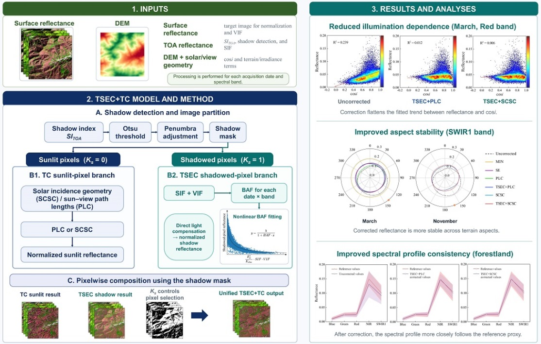
• The proposed TSEC+TC framework partitions rugged-terrain correction into a TC-based sunlit branch and a TSEC-derived shadowed-pixel compensation branch, enabling horizontal-surface-equivalent reflectance estimation from a single optical image and DEM data.
• Across ten Landsat 8 OLI scenes, TSEC+SCSC weakened the relationship between reflectance and illumination, reduced variation among aspects, improved correction in shadow, and increased land cover classification accuracy compared with conventional TC methods.

What are the implications of the main findings?

• Explicitly accounting for self shadows and cast shadows can make topographic normalization more stable in rugged mountainous areas, especially under low solar elevation conditions where conventional TC methods may leave dark pixels or introduce outliers.
• The partitioned framework is modular and showed preliminary applicability to Sentinel-2 MSI and GF-1 WFV imagery, supporting more reliable mountain remote-sensing products without requiring synchronized auxiliary irradiance observations.

Abstract

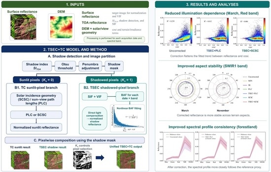
Optical remote sensing images acquired in rugged mountains are affected by reflectance distortion caused by both topography and shadows. Most topographic correction (TC) methods normalize sunlit slopes but can become unstable in self shadow and cast shadow, where little or no direct solar radiation reaches the surface. This study builds on the topographic shadow effect correction (TSEC) model and develops TSEC+TC, a partitioned framework for horizontal equivalent normalization. Using a shadow mask extended to penumbra, the framework integrates TSEC for shadowed pixels with conventional TC for sunlit pixels. Both branches target horizontal equivalent reflectance, enabling simultaneous correction of topographic and shadow effects across the scene. We implemented TSEC+TC with path length correction (PLC) and SCS with C (SCSC) models and evaluated it using ten multi-temporal Landsat 8 OLI scenes under different illumination conditions. The results showed that TSEC+TC reduced terrain-related brightness variation and improved land cover classification in the auxiliary comparison relative to uncorrected and TC-only results. For TSEC+SCSC, the R² values between corrected reflectance and cosi were below 0.025 for both Red and SWIR1 bands, and the coefficient of variation of reflectance across aspects was consistently lower than the corresponding values for SE and SCSC, with a maximum of 36.00%. Shadow area analyses indicated that TSEC+TC compensated reflectance distortion in self shadow and cast shadow areas, reduced TC-induced outliers, and better preserved spectral patterns than TC-only correction. Tests using Sentinel-2 MSI and GF-1 WFV imagery provided preliminary evidence of applicability to other sensors. Accounting for the topographic shadow effect improved TC performance in complex mountainous areas.

1. Introduction

Mountains are complex ecosystems with important ecological functions, including biodiversity conservation, regional climate regulation, and water conservation; therefore, they are important areas for global change research [1,2,3]. Because of the extensive coverage and diverse vegetation types of mountainous areas, remote sensing technology is an important tool for assessing land cover types, vegetation biophysical parameters, and vegetation phenology in these areas [4,5,6,7]. Remote sensing technology also enables large-scale, multi-frequency, and long-term observation of the land surface, and is therefore useful for mountain studies. However, for optical remote sensing, accurately reproducing the surface reflectance is a major challenge in quantitative remote sensing in mountainous areas [8,9].

Terrain relief and solar illumination redistribute solar radiation in mountainous areas. As a result, mountain slopes receive different amounts of solar radiation depending on their orientation [10,11]. Sun-facing slopes generally receive the most radiation. As the slope orientation changes, the amount of solar radiation progressively decreases. Moreover, the terrain slope influences the solar radiation intensity received at the surface [12,13]. The same feature can therefore show different reflectance values in the same image because irradiance varies; this phenomenon is called the topographic effect [14,15,16].

In complex mountainous terrain where there is substantial relief, sun-facing slopes (i.e., sunny slopes) receive solar radiation consisting of direct solar radiation, sky-scattered radiation, and reflected radiation from the adjacent terrain. In contrast, slopes facing away from the sun (i.e., shady slopes) and slopes obscured by other mountains in the direction of the sun’s radiation receive only sky-scattered and terrain-reflected radiation [17,18,19,20]. The energy of sky-scattered and terrain-reflected radiation is considerably less than that of direct solar radiation. Consequently, these areas have very low reflectance in remote sensing images and appear as shadows; this phenomenon is commonly referred to as the topographic shadow effect [21,22,23]. Although this effect falls under the category of topographic effects, it differs from the general topographic effect because it is mainly controlled by illumination loss and is more visually prominent in remote sensing images. For brevity, the topographic shadow effect is henceforth referred to as the shadow effect.

Several topographic correction (TC) methods have been developed to address the topographic effect in mountainous areas. These methods can be summarized into three categories [24,25,26]. The first category comprises simple empirical statistical methods. These methods establish an empirical model based on the relationship between the solar incidence angle and reflectance. Although this method requires few input parameters, the model lacks a physical explanation and is not widely accepted in the remote sensing community. Two representative methods of this category include the statistical-empirical (SE) [27] and variable empirical coefficient algorithm (VECA) [28] models. The second category refers to the physical modeling approach, which has a complete physical basis; however, the complexity of the models within this category varies considerably. For example, the cosine (COS) [27], sun-canopy-sensor (SCS) [29], and path length correction (PLC) [30] models mainly account for direct solar radiation, and their expressions are simple and straightforward to implement. In contrast, models that consider the three components of solar radiation require many model parameters and involve a complicated correction process. Examples of these methods include the Proy [31] and Sandmeier [20] models. The third category encompasses a semi-empirical modeling method that incorporates empirical parameters. This method combines the advantages of the two aforementioned methods and introduces correction parameters with specific physical explanations to construct the model. It therefore has a relatively simple form, is easy to implement, and usually produces reliable correction results. Representative methods in this category include C correction (CC) [27], sun-canopy-sensor with C (SCSC) [32], Minnaert (MIN) [33] and pixel-based Minnaert (PBM) [34] models. Different TC models produce different correction effects; however, most of them mainly eliminate the topographic effect rather than improve the shadow effect in images.

The combined influence of terrain and illumination in mountainous areas produces both topographic and shadow effects. It is difficult to separate these effects, particularly in complex mountainous areas. This makes reliable correction difficult in complex mountainous areas when traditional topographic correction methods are used. In recent years, several studies have focused on the shadow effect. Jiang et al. [35] developed the shadow-eliminated vegetation index (SEVI) to reduce the shadow effect (including self shadow and cast shadow). However, this method lacks a strong physical basis. Yang et al. [36] introduced a shadow intensity factor and developed the NDVI topographic shadow effect correction (NTSEC) model to correct NDVI in areas with strong shadow effect by considering the radiation difference between sunlit and shadow areas. This method has a definite physical basis. Both methods account for the topographic shadow effect. However, the SEVI is unable to correct surface reflectance, whereas the NTSEC model cannot correct surface reflectance effectively. Zhao et al. [37] proposed a downwelling shortwave radiation-based correction (DSRC) method to correct surface reflectance, which is capable of correcting topographic effect and improving the shadow effect. However, this method requires the spatial downscaling of downwelling shortwave radiation data at a 3-km resolution, which inevitably introduces some errors and uncertainties. The DSRC method may also overestimate inherent vegetation reflectance, thereby limiting its applicability.

In our previous study, we proposed the topographic shadow effect correction (TSEC) method [38], which uses shadow intensity, vegetation information, and band adjustment factors to compensate for reflectance loss in self shadow and cast shadow areas. Although TSEC effectively restores shadowed reflectance, its original formulation does not explicitly normalize the results to horizontal surface equivalent reflectance, limiting its integration with conventional TC for sunlit terrain.

To address this issue, this study proposes TSEC+TC, a partitioned topographic normalization framework. The shadow intensity factor was refined to account for penumbra, and BAF was fitted at the scene level to facilitate integration with conventional TC. The revised TSEC branch estimates horizontal surface equivalent reflectance for shadowed pixels, while conventional TC estimates the same target for sunlit pixels. Their combination improves radiometric consistency and continuity across sunlit and shadowed terrain. The framework was evaluated using ten multi-temporal Landsat 8 OLI images acquired under different illumination conditions, followed by preliminary tests on Sentinel-2 MSI and GF-1 WFV imagery.

2. Research Area and Data

2.1. Study Area

The study area is located in the mountainous area between the Anqing and Lu’an cities, Anhui Province, China, at longitude 116°2′30″–116°19′13″E and latitude 31°1′33″–31°16′4″N. The altitude in the area ranges from 101 m to 1747 m, resulting in rugged terrain. Terrain relief in this area produces both a topographic effect and a shadow effect caused by surrounding mountains. The study area also includes several land cover types, including forestland, grassland, cultivated land, shrubland, water body, and shoaly land. It is also located in the mid-latitudes, where vegetation shows clear phenological variation. These conditions make correction difficult and provide a useful test for the proposed method.

2.2. Data

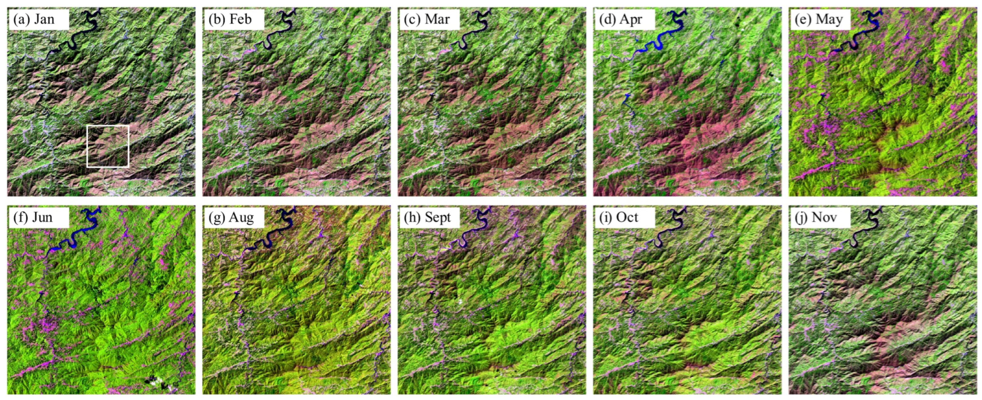
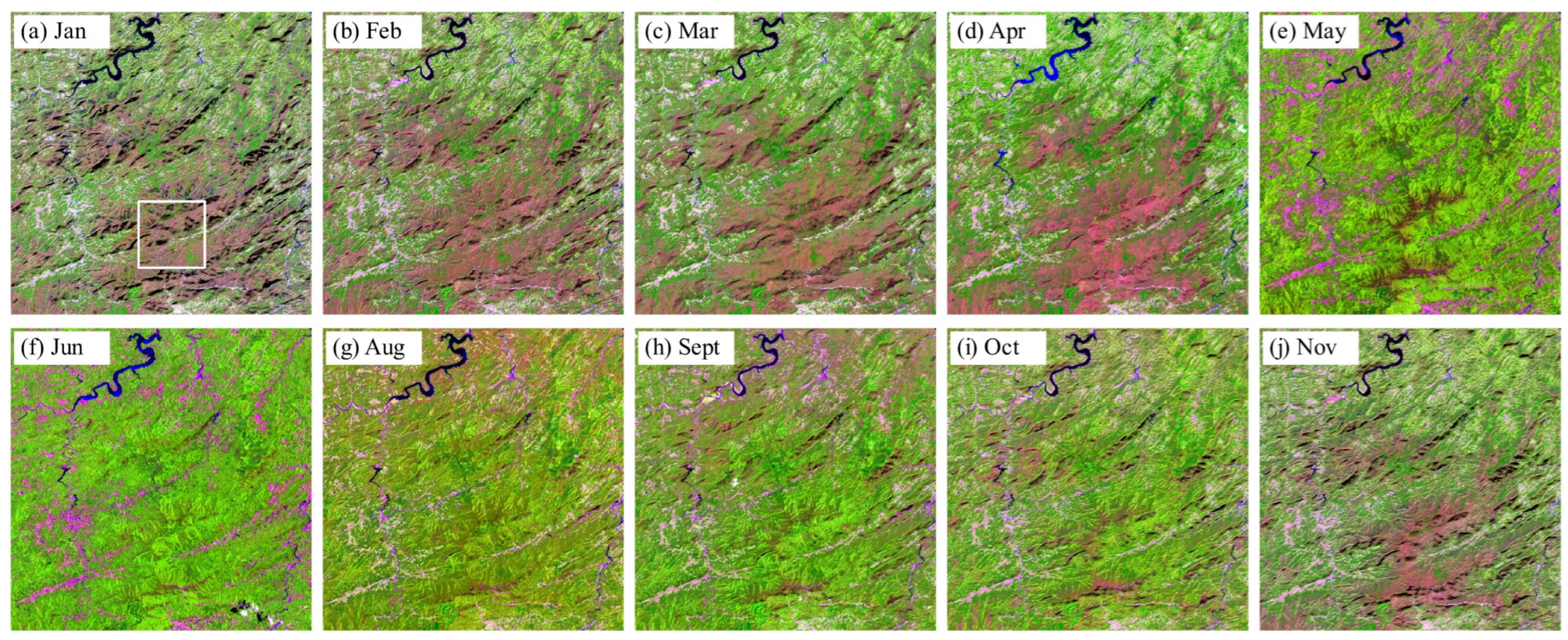
The data supporting this study included two major categories. The first category consisted of imagery data, the majority of which were Landsat 8 OLI images from the U.S. Geological Survey (USGS, https://espa.cr.usgs.gov/). We acquired ten scenes of nearly cloud-free study area images, including top-of-atmosphere (TOA) and surface reflectance data, and covering 10 months between 2020 and 2023 (Figure 1).

Table 1. List of Landsat 8 OLI scenes with their solar elevation and azimuth angles.

Acquisition Date	Solar Elevation (°)	Solar Azimuth (°)
19 January 2021	32.93	152.48
26 February 2023	42.86	145.20
14 March 2023	48.62	141.76
7 April 2023	57.36	135.38
9 May 2023	66.07	122.26
10 June 2023	68.76	108.92
28 August 2020	59.84	132.47
11 September 2022	56.49	139.79
13 October 2022	46.83	152.94
6 November 2022	39.42	157.92

lists the general information on the scenes used, showing the image acquisition date as well as the solar elevation and azimuth angles. The scenes cover different solar elevations and azimuth angles. As the solar elevation angle decreases, the topographic and shadow effects in the images become more pronounced. Using multiple scenes helps assess the applicability and stability of correction methods [26].

The second category was ancillary data, including topographic data, land cover types, and illumination observation products. The topographic data for Landsat 8 were derived from the Advanced Spaceborne Thermal Emission and Reflectance Radiometer (ASTER) Global Digital Elevation Model (GDEM) version 2 product [39], which has a spatial resolution of 30 m. The topographic data for Sentinel-2 and GF-1 consisted of PALSAR DEM data with a spatial resolution of 12.5 m, which were downloaded from the Alaska Satellite Facility Distributed Active Archive Data Center (ASF DAAC). Land cover data were provided by the Data Center for Resources and Environmental Sciences, Chinese Academy of Sciences. The USGS also provides pixel-wise illumination observation products (including solar zenith, solar azimuth, viewing zenith, and viewing azimuth angles), which are important parameters for input into the PLC model [30].

3. Methods

3.1. Topographic Shadow Detection in Images

The impact of the terrain on remote sensing images appears mainly in two ways. The first and most apparent effect is image shadowing caused by mountains blocking sunlight. The second effect is the uneven distribution of radiation in mountainous areas. The combined effect of these two processes leads to reflectance distortion (spectral aberration) in the remote sensing images of mountainous areas. Therefore, before correcting surface reflectance, shadow detection should be performed to identify the areas affected by topographic shadows in the image [36,40].

It is harder to separate shadow and sunlit areas in surface reflectance than in TOA reflectance. We therefore used a TOA shadow index. In Landsat 8 OLI, the Coastal band has the shortest wavelength and a strong atmospheric scattering contribution, while the NIR band shows a marked contrast between shadowed and sunlit vegetation. Combining these bands improves shadow discrimination [41,42]. When a suitable Coastal band was unavailable, the Blue band was used as a substitute, as evaluated for GF-1 WFV in Section 4.7 and Section 5.3.

Based on the abovementioned properties of shadows, we used a TOA reflectance shadow index (SI_TOA) to enhance shadow areas and suppress sunlit areas. For Landsat 8 multispectral remote sensing data, SI_TOA is expressed as follows:

$$S{I}_{TOA}={\displaystyle \frac{{\rho }_{Coastal}^{TOA}-{\rho }_{Green}^{TOA}}{{\rho }_{NIR}^{TOA}}}$$

(1)

where ${\rho }_{Coastal}^{TOA}$, ${\rho }_{Green}^{TOA}$, and ${\rho }_{NIR}^{TOA}$ are the TOA reflectance values in the Coastal, Green, and NIR bands, respectively. Water bodies were masked before shadow detection to avoid their interference. The threshold c was calculated by Otsu’s method [43]. The TSEC shadow index assessment reported in [38] achieved recall and precision above 90%.

Penumbral pixels at the boundary between sunlit and shadow areas receive only part of the direct solar radiation and usually have intermediate reflectance. They were therefore included in the shadow area [44,45,46]. To include these pixels, the Otsu threshold c was shifted toward the sunlit side, and the index value at the shifted boundary was denoted as ${\mathit{SI}}_{\mathit{TOA}}^{\mathit{ac}}$. Pixels with SI_TOA ≤ ${\mathit{SI}}_{\mathit{TOA}}^{\mathit{ac}}$ were classified as sunlit, whereas the remaining pixels were classified as shadow.

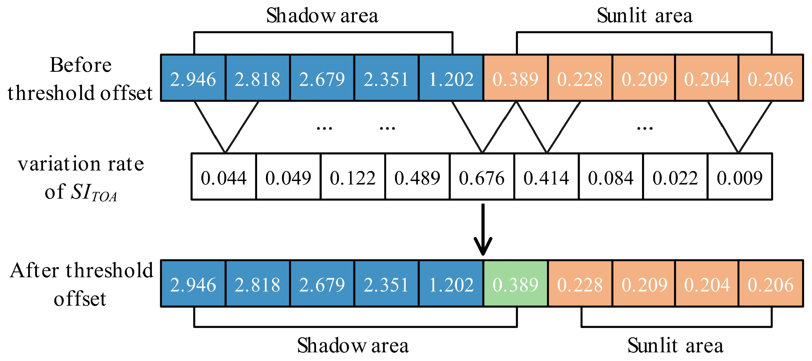
We first used c to divide shadow and sunlit areas in each scene and then examined 50 transects crossing this boundary. Each transect contained five shadow pixels and five sunlit pixels. The pixelwise variation rate was calculated as v_i = |l_i+1 − l_i|/l_i [47]. In the representative profile in Figure 2, the largest change (v_i = 0.676) occurs between SI_TOA values 1.202 and 0.389, which is the boundary identified by c. The change on the sunlit side remains high (v_i = 0.414 between 0.389 and 0.228), while subsequent changes among fully sunlit pixels are 0.084 or lower. We therefore treated the pixel with SI_TOA = 0.389 as penumbra and moved the boundary by one pixel toward the sunlit side, between 0.389 and 0.228. Across the ten scenes, ${\mathit{SI}}_{\mathit{TOA}}^{\mathit{ac}}$ was generally close to the midpoint between the SI_TOA histogram peak and the Otsu threshold. The mask extent associated with five candidate thresholds is examined in Section 5.2.

Therefore, the shadow and sunlit areas can be divided based on the ${\mathit{SI}}_{\mathit{TOA}}^{\mathit{ac}}$ values as follows:

$$K_s=\left\{\begin{array}{l} 1 \mathrm{if} S{I}_{TOA}>S{I}_{TOA}^{ac}\\ 0 \mathrm{otherwise}\end{array}\right.$$

(2)

where K_s is a binary factor: K_s = 1 denotes a shadow pixel, and K_s = 0 denotes a sunlit pixel.

3.2. Physical Target and Partitioned TSEC+TC Formulation

This subsection reformulates the direct light compensation mechanism of TSEC for the shadowed pixel branch of the partitioned TSEC+TC framework and defines its horizontal equivalent reflectance target. All quantities are written for an arbitrary pixel and spectral band, and pixel and band subscripts are omitted for readability. The complete construction and validation of SIF, VIF, and BAF are provided in [38]; only their roles in the present framework are summarized here.

For a rugged surface, the incident irradiance received by a pixel can be decomposed into direct solar radiation, sky-scattered radiation, and terrain-reflected radiation:

$$E=E_d^t\cdot \cos i+E_f^h\cdot V_d+E_h\cdot {\rho }_a\cdot C_t$$

(3)

where $E_d^t$ is the direct solar irradiance transmitted through the atmosphere, $E_f^h$ is the sky-scattered irradiance over a horizontal surface, V_d is the sky view factor, E_h is the total irradiance on horizontal ground, ρ_a is the mean reflectance of adjacent terrain, and C_t is the terrain configuration factor. The cosine of the solar incidence angle is

$$\cos i=\cos {\theta }_z\cos {\theta }_s+\sin {\theta }_z\sin {\theta }_s\cos \left(\phi -\beta \right)$$

(4)

where θ_z represents the solar zenith angle, θ_s denotes the slope angle, φ refers to the solar azimuth angle, and β indicates the aspect angle.

$$E_{shw}=E_f^h\cdot V_d+E_h\cdot {\rho }_a\cdot C_t$$

(5)

Here, E_shw represents the non-direct irradiance baseline formed by the sky-scattered and terrain-reflected components. This approximation closely represents full self shadow and cast shadow conditions. Penumbral pixels may retain residual direct illumination; its contribution is accommodated by the continuous control function f(CF), mainly through SIF.

Let E_H denote the effective reference irradiance for the horizontal equivalent target produced by the sunlit TC branch. The shadowed pixel estimate aligned with this target is denoted as ${\widehat{\rho }}_{shw}^H$. Under the Lambertian approximation and after atmospheric path radiance removal, the surface-leaving radiance of a shadowed pixel and its observed reflectance satisfy

$$L_{shw}={\displaystyle \frac{{\widehat{\rho }}_{shw}^H{E}_{shw}}{\pi }}$$

(6a)

$${\rho }_{shw}={\displaystyle \frac{\pi L_{shw}}{E_H}}={\widehat{\rho }}_{shw}^H{\displaystyle \frac{E_{shw}}{E_H}}$$

(6b)

Combining Equations (6a) and (6b) yields

$${\widehat{\rho }}_{shw}^H={\rho }_{shw}{\displaystyle \frac{E_H}{E_{shw}}}={\rho }_{shw}+{\rho }_{shw}{\displaystyle \frac{E_H-E_{shw}}{E_{shw}}}$$

(7)

The second term is the reflectance increment required to express the shadowed pixel relative to the horizontal equivalent target. Defining the corresponding effective irradiance deficit as

$$\Delta E^H=E_H-E_{shw}$$

(8)

the exact compensation form under the adopted normalization relation is

$${\rho }_{dc}^H={\rho }_{shw}{\displaystyle \frac{\Delta E^H}{E_{shw}}}$$

(9)

Although Equation (9) is exact under the adopted normalization relation, $\Delta E^H$ is not directly observable from a single image. Because E_shw already represents the non-direct irradiance baseline, $\Delta E^H$ is dominated by the direct light component absent in full shadow or only partially available in penumbra. The normalized effective missing direct light fraction is therefore defined as

$${\eta }^H={\displaystyle \frac{\Delta E^H}{E_d^t}},\Delta E^H={\eta }^H{E}_d^t$$

(10)

The dimensionless term ${\eta }^H$ represents the fraction of the direct light energy scale that must be restored. It absorbs direct light visibility, residual illumination in penumbra, shadow severity, projection geometry, band dependence, and surface information constraints. Since ${\eta }^H$ is not directly observable, it is approximated by the TSEC control function:

$${\eta }^H\approx f(CF)$$

(11)

with

$$f(CF)=SIF\cdot VIF\cdot BAF$$

(12)

Substituting Equation (11) into Equation (9) gives the TSEC-derived effective direct light compensation term:

$${\rho }_{dc}^H={\rho }_{shw}f(CF){\displaystyle \frac{E_d^t}{E_{shw}}}$$

(13)

Here, SIF represents the spatial severity of direct light deficiency, VIF constrains compensation according to vegetation or surface information retained under low-signal conditions, and BAF regulates the band-dependent compensation magnitude. Because K_s already separates shadowed and sunlit pixels in Section 3.1, the compact SIF definition is

$$SIF=K_s{\displaystyle \frac{S{I}_{TOA}-S{I}_{TOA}^{ac}}{S{I}_{TOA}^{\max }-S{I}_{TOA}^{ac}}}$$

(14)

In implementation, SIF is constrained to the range 0–1. The complete construction of the factors follows [38], while Section 3.3 describes the BAF calculation used in the present implementation. The shadowed pixel branch estimate is

$${\widehat{\rho }}_{shw}^H={\rho }_{shw}+{\rho }_{dc}^H$$

(15a)

$${\widehat{\rho }}_{shw}^H={\rho }_{shw}+{\rho }_{shw}f(CF){\displaystyle \frac{E_d^t}{E_{shw}}}$$

(15b)

For sunlit pixels, the selected TC model provides the corresponding horizontal equivalent estimate:

$${\widehat{\rho }}_{sun}^H=TC({\rho }_{sun})$$

(16)

The final TSEC+TC output is obtained by combining the two branch estimates for the same target using the shadow mask:

$${\rho }_{corr}=K_s{\widehat{\rho }}_{shw}^H+(1-K_s){\widehat{\rho }}_{sun}^H$$

(17)

In this formulation, the TSEC-derived output is the estimate for shadowed pixels. The plus sign in TSEC+TC represents the composition of the TSEC shadow branch and the conventional TC sunlit branch, both expressed for the same horizontal equivalent target.

3.3. Calculation of BAF

The BAF formulation builds on TSEC [38]. In the original TSEC procedure, BAF was calibrated from paired samples on adjacent sun-facing and shaded slopes of homogeneous land cover. For the scene-wide implementation of TSEC+TC, the present procedure uses all detected shadow pixels to fit one BAF for each acquisition date and spectral band. This reduces dependence on manually selected samples from a single land-cover type. The resulting BAF is specific to that acquisition date and spectral band and is applied across the corresponding shadow area. Because the ratio between the direct radiation component and the nondirect irradiance baseline varies among dates and spectral bands, a coefficient fitted for one date or band was not transferred to another.

Using the notation defined above, Equation (15b) can be rearranged as

$${\rho }_{shw}={\displaystyle \frac{{\widehat{\rho }}_{shw}^H}{1+BAF\cdot x}}$$

(18a)

$$x={\displaystyle \frac{E_d^t}{E_{shw}}}SIF\cdot VIF$$

(18b)

Here, x is calculated from the known irradiance terms, SIF, and VIF. The nonlinear model used in the analysis is

$$y={\displaystyle \frac{b}{1+ax}}$$

(19)

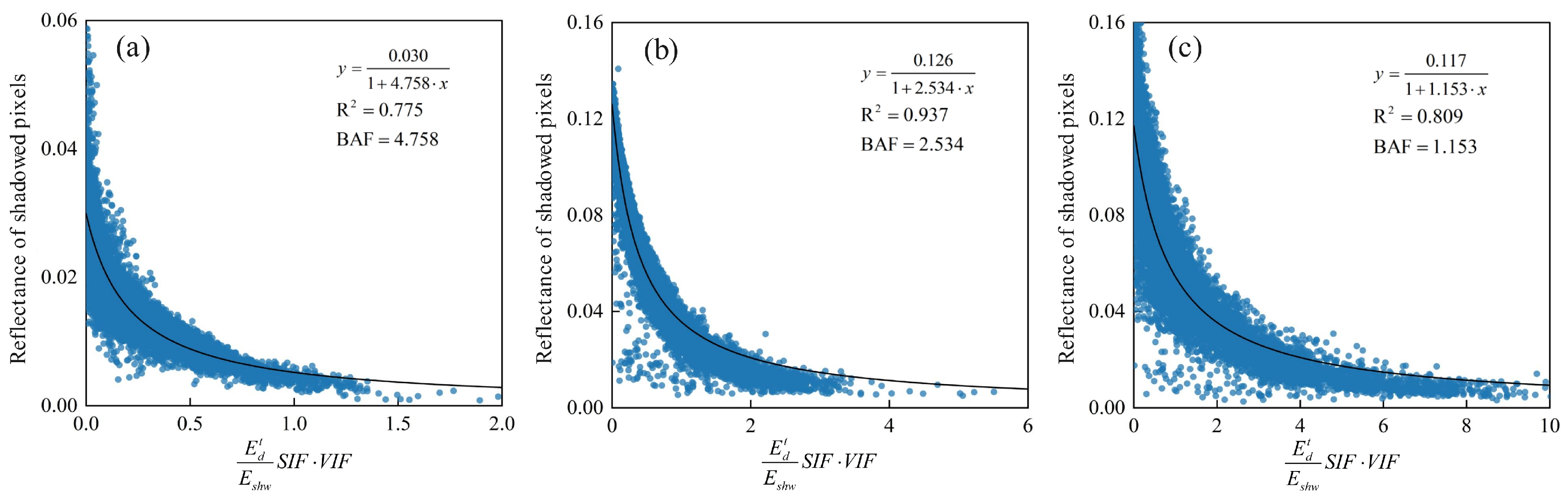
In this model, a represents BAF and b is the fitted horizontal equivalent reflectance parameter. For each date and band, y comprised the original reflectance values for all pixels within the shadow area identified by the mask adjusted for penumbra. Equation (19) was fitted independently for every corrected band and acquisition date using nonlinear least squares. Figure A1 shows representative January fits for the Green, NIR, and SWIR1 bands. The three bands show similar data distributions, and the three illustrated fits have R² values above 0.77, supporting the reliability of the fitted BAF values.

Implementation workflow: (1) calculate the penumbra adjusted mask, SIF, VIF, and irradiance terms; (2) assemble x and y for one date and band; (3) fit Equation (19) and record a as BAF; and (4) apply that BAF to the same date and band, then repeat for the remaining combinations.

3.4. Implementation of the Sunlit Pixel TC Branch and Comparison TC Models

The generic sunlit branch and final partitioned composition have been defined in Equations (16) and (17), respectively. This subsection specifies the TC models used to implement TC(ρ_sun). In this study, the physically based path length correction (PLC) model and the semi-empirical sun-canopy-sensor plus C (SCSC) model were used to generate the sunlit pixel branch ${\widehat{\rho }}_{sun}^H$. In the following TC formulas, δρ denotes the TC-estimated sunlit branch output and corresponds to ${\widehat{\rho }}_{sun}^H$ in Equation (16).

PLC has a sound physical basis and can reproduce vegetation reflectance for sunlit pixels through the following expression [30]:

$$\delta \rho ={\rho }_o\cdot {\displaystyle \frac{S_{sun}+S_{view}}{S_{sun}^t+S_{view}^t}}$$

(20)

where δρ and ρ_o represent the corrected and uncorrected reflectance in the image; S_sun and S_view denote the path lengths along the sun and the viewing direction over flat terrain, respectively; and $S_{\mathit{sun}}^t$ and $S_{\mathit{view}}^t$ refer to the path lengths along the sun and the viewing direction over sloping terrain, respectively. S_sun and S_view were computed as follows:

$$S_{sun/view}={\displaystyle \frac{1}{\cos {\theta }_z}}$$

(21)

$S_{\mathit{sun}}^t$ and $S_{\mathit{view}}^t$ were calculated as follows:

$$S_{sun/view}^t={\displaystyle \frac{1}{\cos {\theta }_z(1-\tan {\theta }_s\cos (\phi -\beta )\tan {\theta }_z)}}$$

(22)

For S_sun and $S_{\mathit{sun}}^t$, θ_z and φ represent the solar zenith and azimuth angles; for S_view and $S_{\mathit{view}}^t$, the corresponding viewing zenith and azimuth angles are used.

SCSC has stable correction performance and is often regarded as a strong TC method. It can be expressed via the following calculation [32]:

$$\delta \rho ={\rho }_o\cdot {\displaystyle \frac{\cos {\theta }_s\cos {\theta }_z+C}{\cos i+C}}$$

(23)

where C represents the ratio of the intercept and slope in the linear regression equation between cosi and ρ_o.

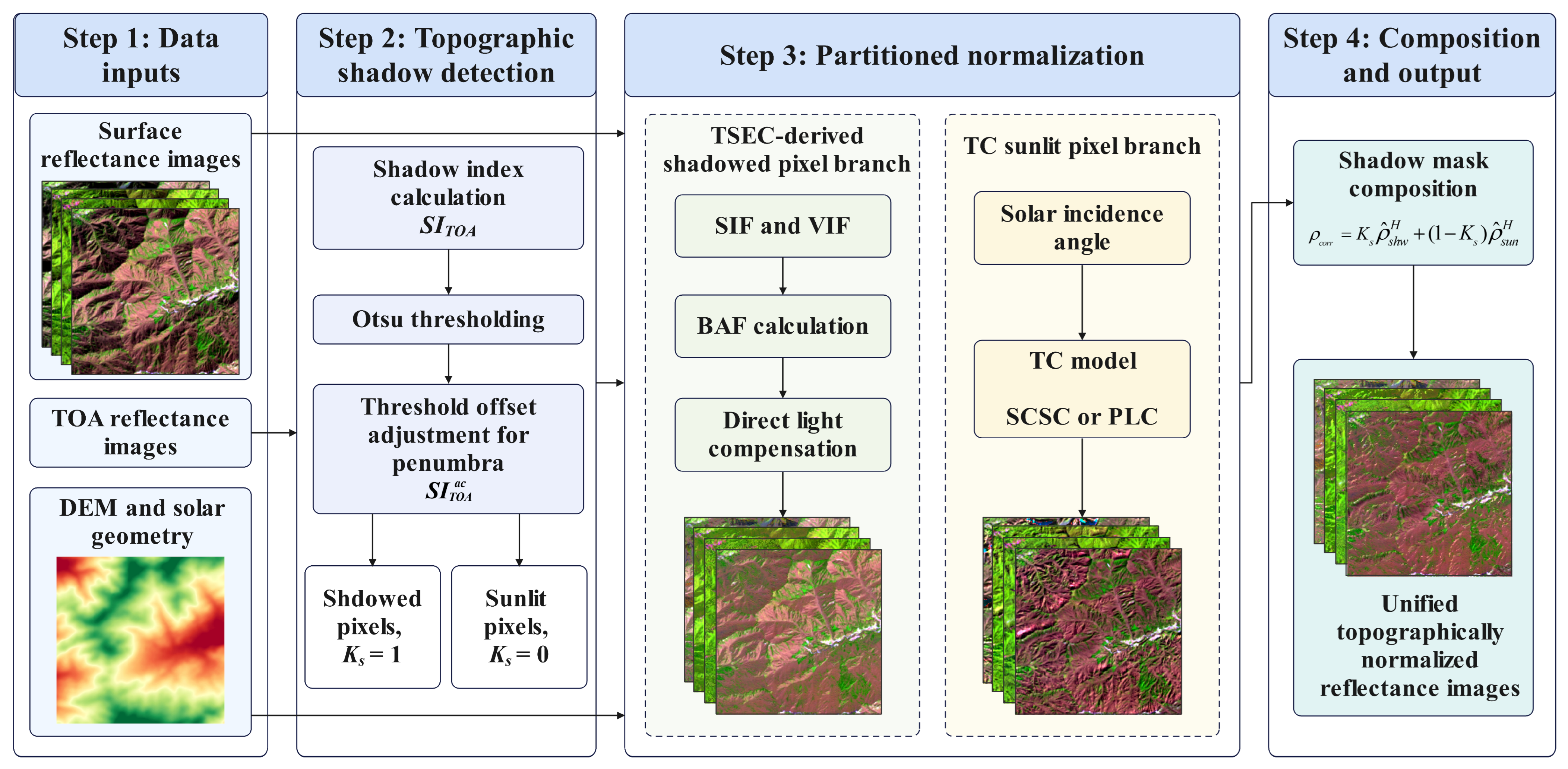
We refer to the version that combines the TSEC shadow branch with PLC as TSEC+PLC, and the version that combines it with SCS+C as TSEC+SCSC. PLC and SCSC were also tested alone. Two further TC models were included for comparison: the statistical empirical (SE) model and the Minnaert (MIN) model, whose expressions are listed in

Table 2. Expressions for the two additional TC methods selected for comparison.

Method	Equation	Source
MIN	$\delta \rho ={\rho }_o\cdot {\displaystyle \frac{\cos {\theta }_s}{{(\cos i\cdot \cos {\theta }_s)}^k}}$	[33]
SE	$\delta \rho ={\rho }_o-\left(b+m\cdot \cos i\right)+{\overline{\rho }}_o$	[27]

Note: k represents the Minnaert constant; ${\overline{\rho }}_o$ indicates the mean reflectance of the corresponding spectral band.

. The required inputs and the workflow of the two branches are summarized in Figure 3.

4. Results

4.1. Visual Comparison of Correction Results

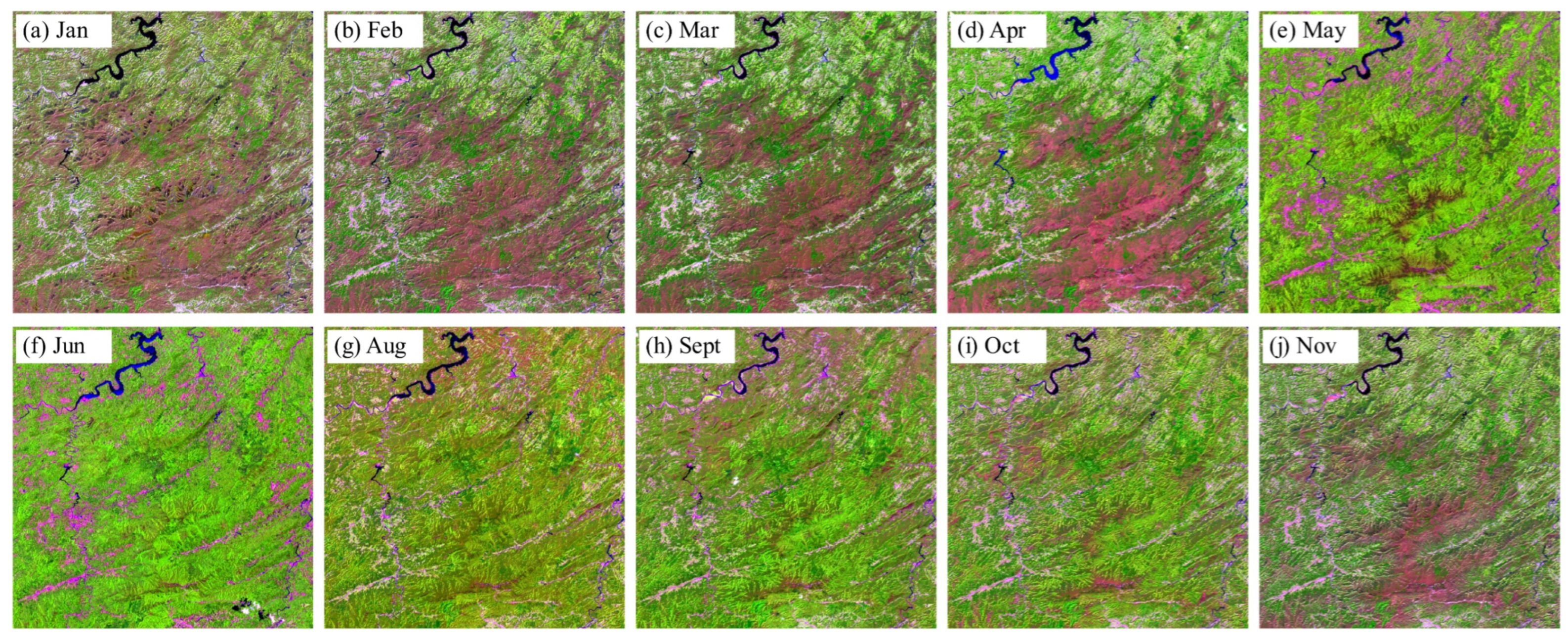
Figure 4 and Figure 5 show the correction results for TSEC+PLC and TSEC+SCSC, respectively. Visual analysis showed that both methods preserved the original color hues (Figure 1) while reducing the terrain relief caused by solar illumination. The shadow areas in the original image were compensated, allowing the colors of the shadow area to approximate those of the surrounding sunlit area. This was evident in the TSEC+SCSC correction results, as the images for each date did not display any noticeable terrain relief or dark pixels.

On dates with low solar elevation angles, some dark pixels appeared in the TSEC+PLC-corrected images (Jan–Mar and Sept–Nov in Figure 4). These dark pixels were mainly located in the sunlit area, which may be related to the correction performance of the PLC method. However, TSEC+PLC yielded slightly better results than the TSEC+SCSC correction for dates with higher solar elevation angles (May–Aug in Figure 4) based on visual inspection. This improvement was mainly attributable to the higher consistency of color information between shady and sunny slopes, as can be observed by comparing the original images (Figure 1).

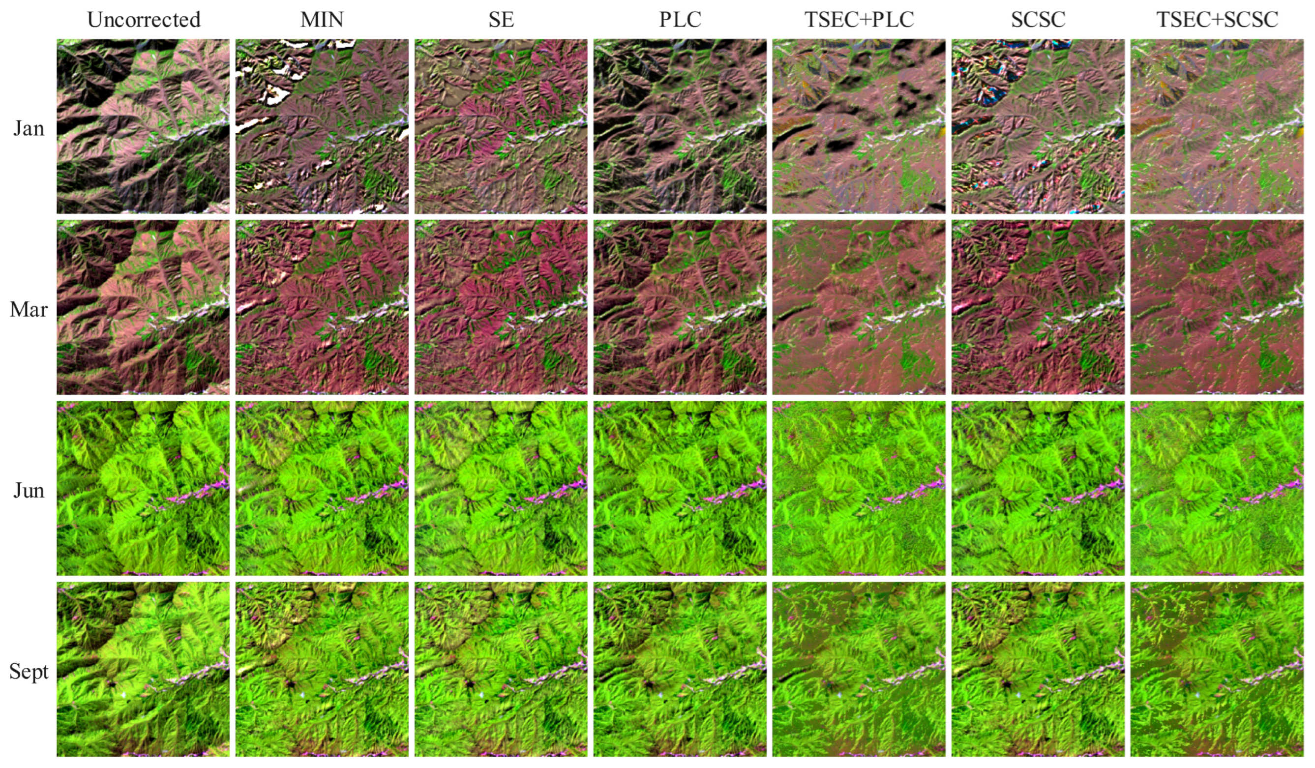
A detailed visual comparison of the subregion (white box in Figure 4) is shown in Figure 6. The proposed method was compared with commonly used TC methods. The correction results for four dates (Jan, Mar, Jun and Sept) were selected because their solar elevation angles represented lower, intermediate, and higher illumination conditions during the year. After correction, terrain-related brightness variation was reduced in most results. For the March image, the correction results of the five TC methods were similar, and the two TSEC+TC implementations also showed comparable visual patterns. However, the TSEC+TC results provided smoother transitions between sunlit and shadowed areas. Because topographic and shadow effects were weak in the June images, all corrected images appeared visually similar to the original images.

4.2. Influence of Illumination Conditions

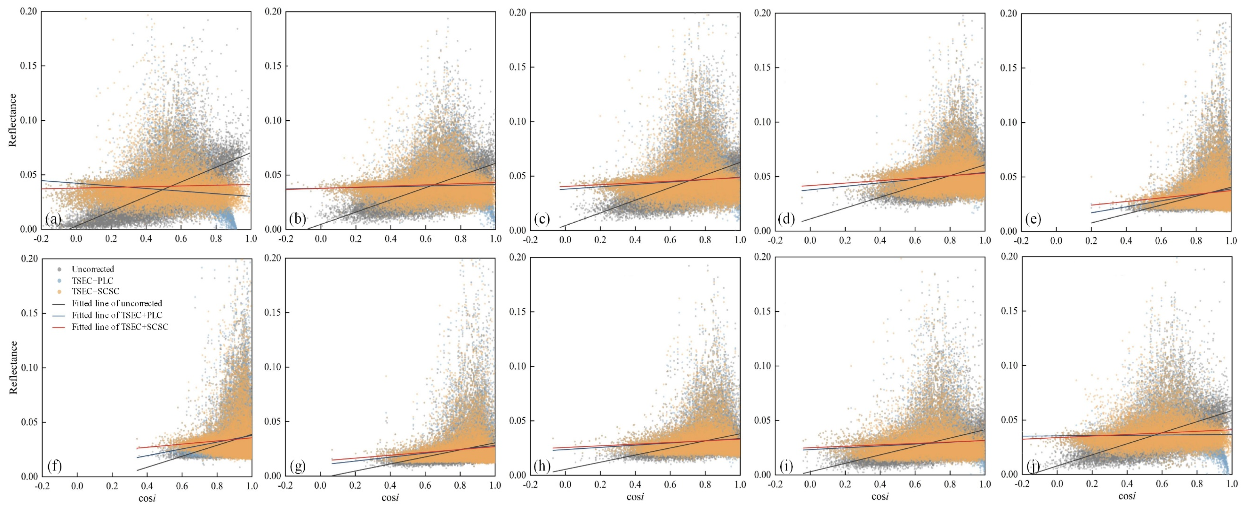
Solar illumination causes both topographic and shadow effects. The change in the correlation between reflectance and illumination conditions before and after correction was used to assess the performance of the correction method. Figure 7 displays the correlation between the reflectance and illumination conditions (cosi) for the Red band, and the coefficients of determination R² are indicated in

Table 3. R² values of the regression between reflectance and cosi before and after correction for each scene.

Dates	Red Band			SWIR1 Band
	Uncorrected	TSEC+PLC	TSEC+SCSC	Uncorrected	TSEC+PLC	TSEC+SCSC
Jan	0.397	0.019	0.002	0.573	0.017	0.007
Feb	0.331	0.002	0.005	0.509	0.008	0.006
Mar	0.239	0.012	0.006	0.432	0.002	0.009
Apr	0.184	0.023	0.011	0.343	0.039	0.012
May	0.078	0.035	0.013	0.218	0.066	0.021
Jun	0.065	0.025	0.006	0.175	0.023	0.001
Aug	0.069	0.023	0.012	0.303	0.043	0.017
Sept	0.113	0.012	0.007	0.347	0.025	0.011
Oct	0.176	0.010	0.006	0.464	0.026	0.016
Nov	0.322	0.000	0.010	0.517	0.006	0.017

(demonstrated for the Red and SWIR1 bands).

The uncorrected image was strongly affected by illumination conditions, showing a clear relationship between reflectance and cosi. In June, when the solar elevation angle was higher, illumination conditions had less influence on reflectance. However, as the solar elevation angle decreased, the influence of the illumination condition on the reflectance gradually became stronger. In particular, for the SWIR1 band, reflectance was strongly influenced by illumination conditions, as reflected by the high correlation between reflectance and cosi before correction. This pattern was most obvious in January when the solar elevation angle was low (as shown in Table 3, with an R² value exceeding 0.5).

After correction, the correlation between reflectance and cosi decreased (Table 3), and the fitted line became nearly horizontal. This indicated a reduction in the influence of illumination conditions on reflectance. The R² values and fitted line tendencies showed that TSEC+SCSC had stronger decorrelation ability than TSEC+PLC. For each date, the R² between reflectance and cosi in the Red and SWIR1 bands corrected by TSEC+SCSC did not exceed 0.025, suggesting stable correction performance.

4.3. Aspect Differences in Reflectance

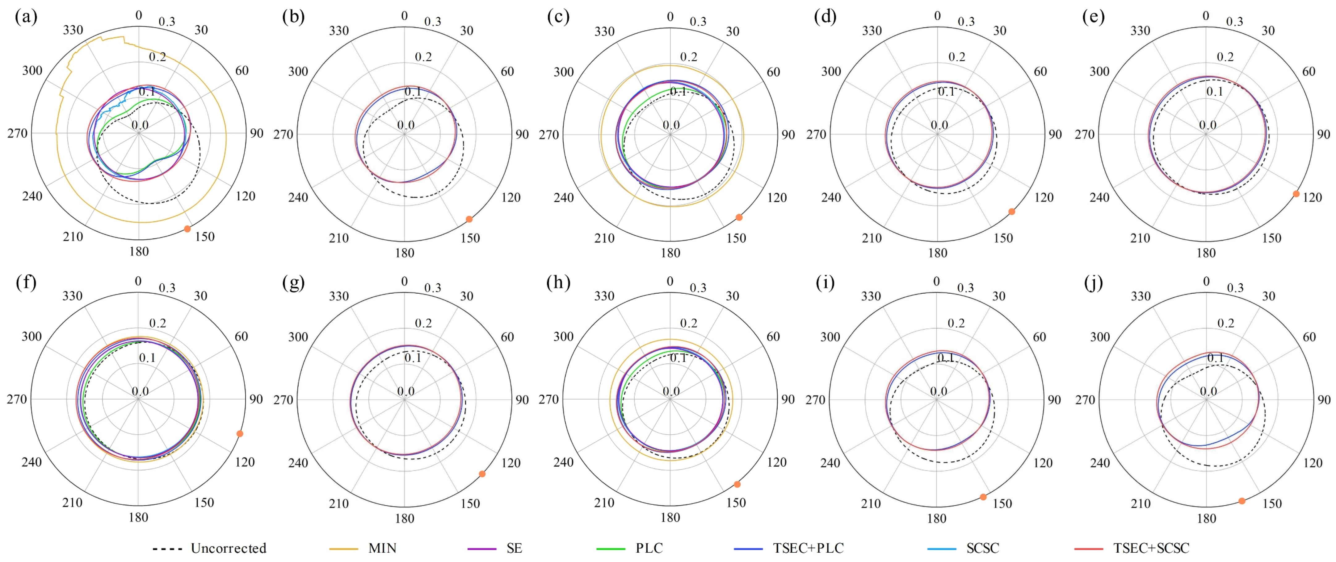
Topographic and shadow effects were also affected by aspect, in addition to sunlight. Slopes facing the sun receive more solar radiation than those not facing the sun. The reflectance value was higher when the slope was closer to the direction of the sun. Therefore, the reflectance values varied with aspect within the uncorrected images. This phenomenon was apparent in the polar plots of the reflectance values. Figure 8 shows the variation in the SWIR1 band reflectance values with aspect before and after correction. The solar direction is marked with orange dots in the figure. The analysis also includes a comparison with TC methods.

Before correction, the reflectance facing the sun was noticeably greater than that in the opposite direction. This resulted in the reflectance curve being biased towards the direction of the sun, exhibiting a clear aspect difference that agrees with the theoretical analysis. As the solar elevation angle increased, the aspect difference before correction gradually decreased, especially for the June image, which was very small, and the reflectance curves before correction coincided with the reflectance curves after correction for each method. In March and September, the aspect differences in reflectance were clearly reduced after correction for each method, and the reflectance curves exhibited a circular shape centered at the origin of the coordinate system. In the January image, the corrected reflectance curves, which had been adjusted by PLC, did not exhibit a rounded shape. In addition, there was a noticeable deviation or “retraction” in both the directions facing the sun and away from the sun (Figure 8a). This suggested that there were varying degrees of undercorrection in both directions, and the method might not be suitable for images with very low solar elevation angles. Although TSEC+PLC addressed undercorrection in the direction away from the sun, the issue of undercorrection in the direction facing the sun remained. The reflectance curves of MIN and SCSC also exhibited large fluctuations in the direction away from the sun (approximately 295–350°). This suggests that these three methods may be unable to consistently correct the reflectance of shady slopes facing away from the sun. TSEC+SCSC did not exhibit this phenomenon and addressed the shortcomings of SCSC, resulting in well-maintained corrected reflectance curves.

A closer examination of Figure 8 showed that the reflectance curve areas differed among correction methods, especially for the January image. Ideally, correction methods should not significantly alter the area of the circle because the radius should decrease and increase in the directions facing the sun and away from the sun, respectively [30,48]. To quantify the correction stability, we calculated the area of the curve enclosed by the reflectance in the polar plot before and after correction for the four dates and then calculated the relative error (RE) of the circle’s area as well as the coefficient of variation (CV) of the reflectance, as shown in

Table 4. RE (%) and CV (%) of reflectance for different aspects before and after correction.

Correction Method	Jan		Mar		Jun		Sept
	RE	CV	RE	CV	RE	CV	RE	CV
Uncorrected	-	61.36	-	38.02	-	21.18	-	26.48
MIN	86.85	434.16	33.67	31.20	7.69	19.04	17.24	21.84
SE	−3.49	40.17	−1.37	28.57	−0.32	19.32	−1.06	21.45
PLC	−19.18	66.70	−5.18	33.39	−0.83	20.10	−2.76	23.31
TSEC+PLC	−2.80	47.71	2.22	25.15	4.31	17.21	2.25	19.13
SCSC	−4.28	556.22	−0.10	30.23	−0.22	19.45	−0.42	21.78
TSEC+SCSC	4.94	36.00	2.20	26.20	4.27	17.11	2.30	19.17

. Since CV is calculated as SD/mean × 100%, the extremely high CV values observed for MIN and SCSC were mainly caused by negative or near 0 mean reflectance values under low illumination conditions, which caused the denominator to approach 0. The SE and SCSC methods produced low RE values on all four dates, with SCSC reaching −4.28% and SE reaching −3.49% in January. The TSEC+PLC and TSEC+SCSC methods showed similar RE behavior, with maximum RE values not exceeding ±5%. These findings indicate that the TSEC+TC-corrected reflectance did not substantially change the overall polar plot area and was consistent with improved aspect stability. Together, these results indicate stable topographic normalization, because the TSEC+TC-corrected reflectance was not obviously overestimated or underestimated. The TSEC+PLC and TSEC+SCSC methods generally exhibited greater stability with lower CVs than the SE and SCSC methods, except that the January TSEC+PLC CV was higher than that of SE.

4.4. Correction Performance in the Shadow Area

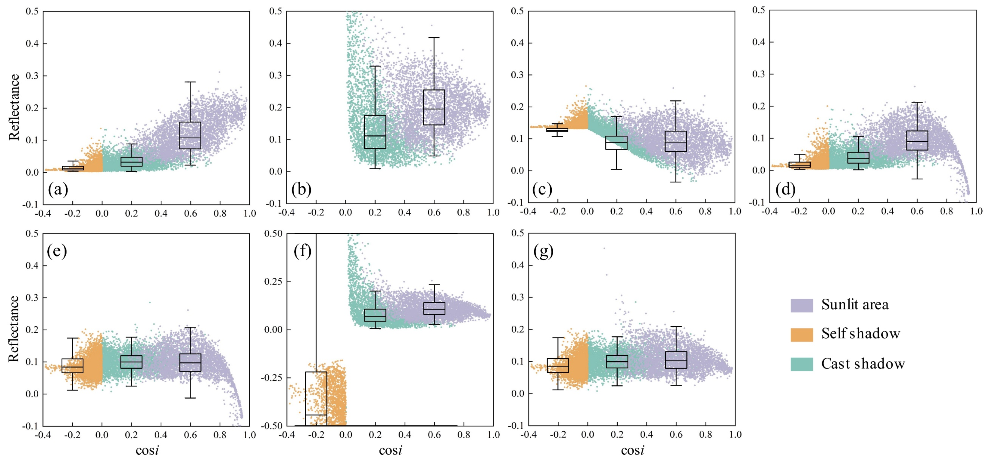
In mountainous areas, shadows are formed when sunlight is blocked by a mountain. They can be categorized as self shadows and cast shadows, according to the cause of the shadow. A self shadow is an area that is not directly illuminated by sunlight (i.e., the side of the mountain facing away from the sun), and a cast shadow is a shadow that is cast on the background of the scene when the mountain is blocked in the direction of the light source. Most of the shadows in the remote sensing image belong to the cast shadow category. These are present in almost every remote sensing image acquired in mountainous areas. However, for areas with high terrain relief, there are also prominent self shadows in the image. We divided shadows into self shadow and cast shadow according to their formation. Self shadow was identified directly as cosi ≤ 0 using Equation (4). The remaining pixels within the shadow mask were classified as cast shadow.

To quantitatively evaluate the performance of the TSEC+TC method in shadowed areas, we sampled 10,800 forestland pixels from the January image. The samples included 3600 pixels each in the sunlit, self shadow, and cast shadow areas, which were selected based on land cover type data. Figure 9 shows the scatter distributions of reflectance with cosi before and after correction for the five TC methods and the two TSEC+TC methods, using the SWIR1 band as an example. The boxes from left to right represent the sunlit area, self shadow, and cast shadow areas, respectively.

The reflectance values of both self shadow and cast shadow pixels were low before correction, whereas those of sunlit pixels were high. In addition, the reflectance scatter of the sunlit area decreased with decreasing cosi. After correction, the reflectance scatter in the sunlit area tended to be horizontally distributed, indicating that all methods reduced illumination-related variation in sunlit pixels. However, MIN was unable to correct self shadow pixels owing to its expression defects (Figure 9b); these uncorrected self shadow areas correspond to the blank spaces in Figure 6. This defect limited the applicability of MIN to complex mountainous terrain. SCSC also produced inadequate self shadow correction results because many corrected reflectance values became negative. In addition, MIN and SCSC overcorrected pixels when cosi was close to 0. PLC suppressed overcorrection more effectively, but it remained weak in correcting both self shadow and cast shadow pixels. A few directly sunlit pixels also appeared to be reverse-corrected.

Some studies suggest that SE is more suitable than other TC methods for complex mountainous terrain, which is consistent with the first three analyses in this section. Nevertheless, the correction performance in self shadow and cast shadow areas shows substantial limitations of SE. Figure 9c shows that the reflectance point distribution pattern and the range between Q3+1.5IQR and Q1−1.5IQR (1.5IQR range) in the self shadow area after SE correction remained similar to those before correction. In other words, the self shadow reflectance was almost uniformly enhanced, but the result remained physically implausible. Correction of cast shadow reflectance showed similar limitations. Because SE corrects reflectance by fitting a linear empirical relationship with cosi, the corrected reflectance in cast shadow areas increased with lower cosi and formed a linear trend. This result conflicts with the expectation that the intrinsic spectral properties of a feature should not change simply because the solar illumination condition changes. Although the SE correction results appear visually acceptable, this method is less suitable for quantitative surface reflectance correction in mountainous areas because of the limitations of empirical approaches [26,30].

The two TSEC+TC methods reduced both overcorrection and undercorrection, and the reflectance scatters of the corrected sunlit, self shadow, and cast shadow areas tended to be nearly horizontally distributed. Both the global decorrelation of reflectance with illumination condition (see Section 4.2) and the local zone decorrelation were improved, indicating that TSEC+TC mitigated shadow-induced reflectance distortion while normalizing terrain-related variation. The 1.5 IQRs of sunlit, self shadow, and cast shadow reflectances were closely aligned after TSEC+TC. TC methods alone did not achieve this level of consistency. Because surface reflectance should be referenced to a common physical target regardless of whether a pixel is sunlit or shadowed, this result supports the partitioned TSEC+TC framework for estimating a unified normalized reflectance field.

4.5. Improvement of Classification Accuracy

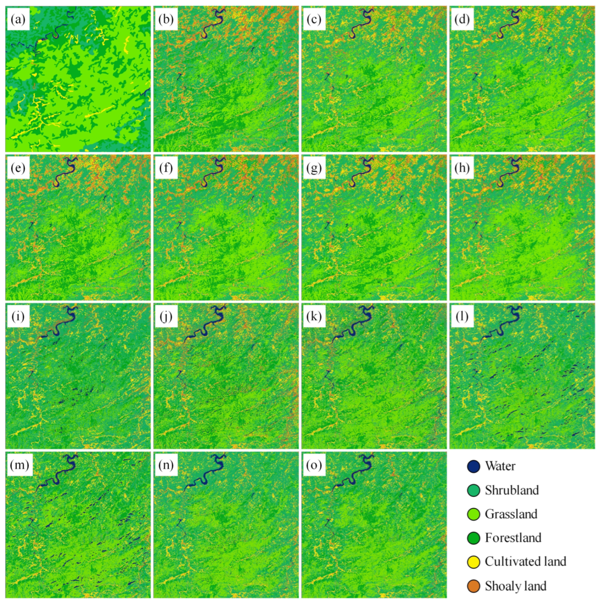
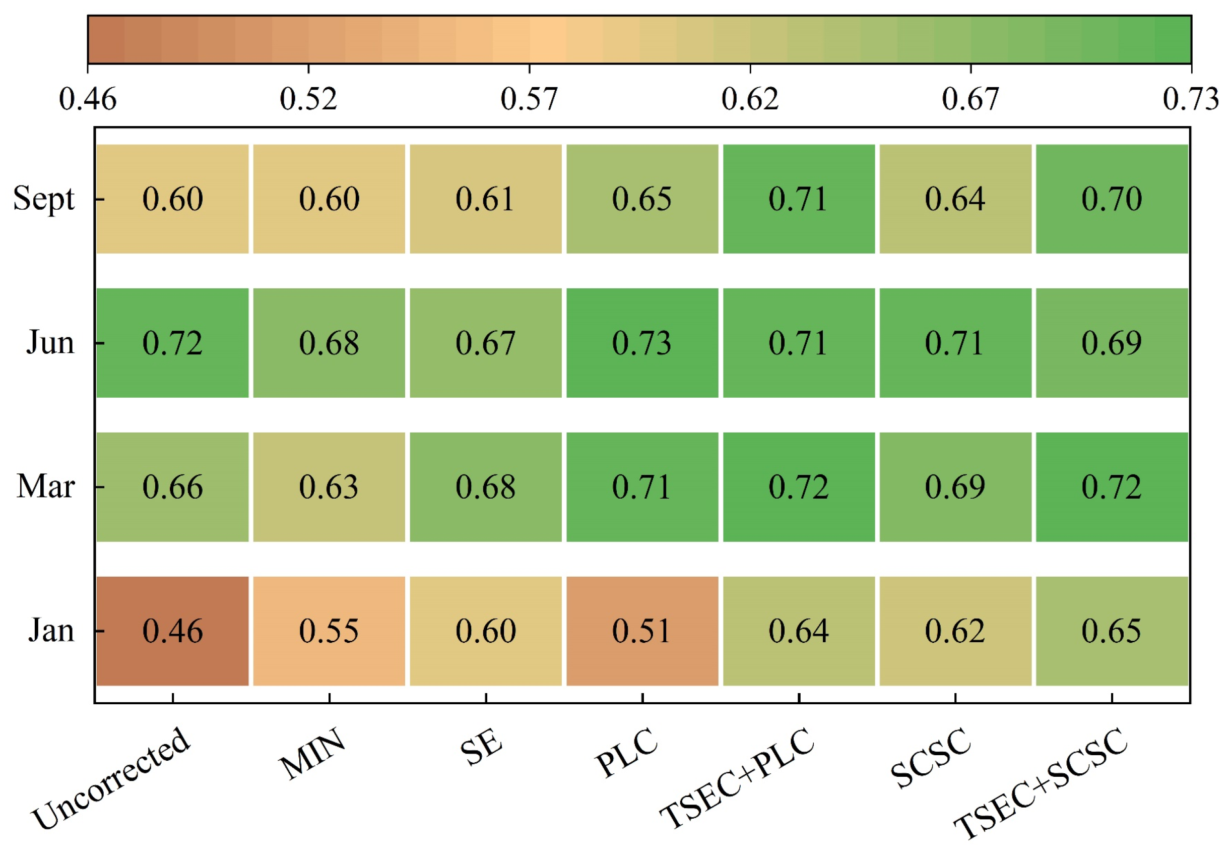
Land cover classification before and after correction provides an auxiliary evaluation of correction effects on thematic products. Only spectral features were used. Classification was pixel based in eCognition, with one pixel represented by one image object. For January, March, June, and September, the same manually selected locations and class totals were retained. Each date used 37,295 training pixels (161 shoaly land, 3512 cultivated land, 13,830 forestland, 15,432 grassland, 4034 shrubland, and 326 water) and 49,746 pixels for accuracy assessment (277, 1661, 13,967, 26,824, 6270, and 747, respectively). The training and accuracy assessment samples were manually delineated as separate sample sets but were not fully mutually exclusive at the pixel level. For each uncorrected or corrected product, a separate Random Tree classifier was trained and applied with the same eCognition default configuration, including a maximum of 50 trees. Figure 10 presents the September and January maps, and Figure 11 compares overall accuracy (OA).

For the January image, the classification results before correction showed severe confusion between forestland, grassland, and shrubland owing to topographic and shadow effects, which explains the very low classification accuracy of the uncorrected images. The TC alleviated the confusion between grassland and shrubland, but considerable confusion persisted between forestland and shrubland. Figure 11 illustrates an increase of approximately 20% in classification accuracy following correction using several TC methods. However, certain shadow areas continued to be misclassified as water due to their similar spectral features, and distinguishing between them becomes complicated when pixels are covered by prominent shadows [41]. After correction by the two TSEC+TC methods, shadow-induced confusion was reduced, thereby improving the separation between forestland, grassland, and shrubland and increasing classification accuracy.

Because shadow areas were almost absent in the June image and the topographic effect was minimal, the correction had little effect on classification accuracy, which was approximately 0.7 after correction for all methods and close to the uncorrected result. Only the PLC-corrected accuracy was higher than the uncorrected accuracy, possibly because PLC reproduced vegetation reflectance more adequately under weak terrain effects. The two TSEC+TC methods produced the highest classification accuracies for all dates except June and showed higher accuracy than the uncorrected results. Across the four dates, TSEC+TC increased classification accuracy from 0.46–0.72 before correction to 0.64–0.72 after correction. Within this auxiliary comparison, these results indicate that mitigating topographic and shadow-induced reflectance distortion before land cover classification can improve classification performance in rugged mountainous areas.

4.6. Horizontal Equivalent Reflectance Estimation and Outlier Analysis

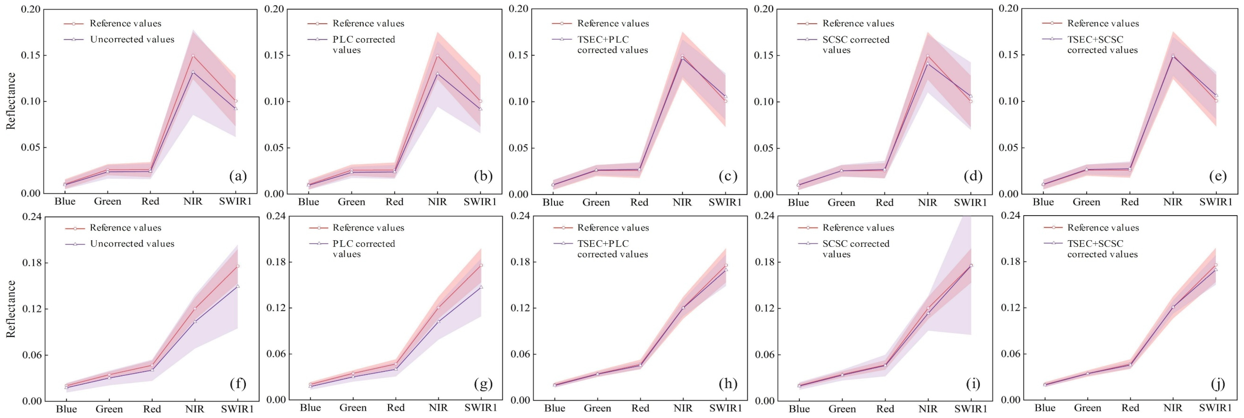
The ability of TSEC+TC to estimate horizontal equivalent reflectance was evaluated in a subregion of the March image, with SCSC and PLC included for comparison (Figure 12). Direct field measurements were unavailable. For forestland and grassland, the mean reflectance of pure sunlit samples after SCSC and PLC was therefore used as a reference proxy specific to each method [30]. These proxies provide internal comparison targets and are not field observations.

Before correction, reflectance in each band was lower than the reference values because of the topographic shadow effect. PLC underestimated its reference, whereas TSEC+PLC brought the reflectance estimates closer to that value. SCSC estimates were close to its reference, but the error range extended beyond the reference range, indicating unstable estimation for some pixels. TSEC+SCSC improved agreement with the SCSC based reference and reduced the spread.

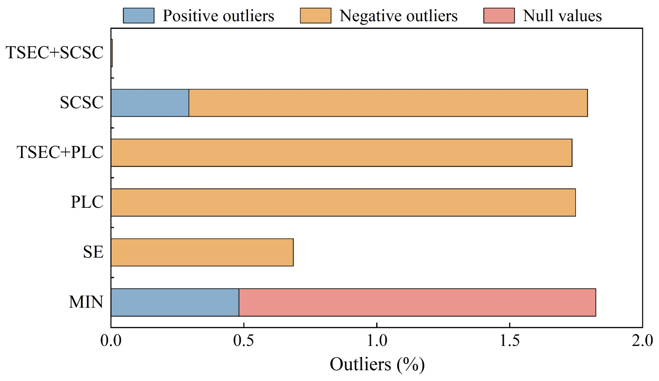
Overcorrection and undercorrection can distort normalized reflectance estimation and produce outliers. Outliers often occur in images with low solar elevation angles. In this study, the SWIR1 band reflectance from the original January image was used as the basis for an outlier definition: corrected values greater than the maximum original reflectance were defined as positive outliers; values less than the minimum original reflectance were defined as negative outliers; and values that could not be corrected were defined as null values [26]. Figure 13 illustrates the outlier statistics. Outliers exceeded 1.5% across all methods except SE and TSEC+SCSC. The null values for MIN were located within self shadow areas. PLC and TSEC+PLC produced nearly the same number of outliers, and both were negative outliers, indicating that combining TSEC with PLC did not introduce additional outliers under this criterion. TSEC+SCSC substantially reduced the outliers produced by SCSC and produced few outliers under the adopted outlier criterion, indicating stable correction behavior compared with the other methods. Because this scene relative criterion is not a universal physical bound, limits defined for specific bands and surface types could provide a complementary test in future work.

4.7. Preliminary Applicability to Other Sensors

The method can be run on other multispectral sensors because it needs one image and a DEM. However, the present evidence consists of only one Sentinel-2 MSI scene and one GF-1 WFV scene from the same region. This section is therefore a preliminary test on other sensors.

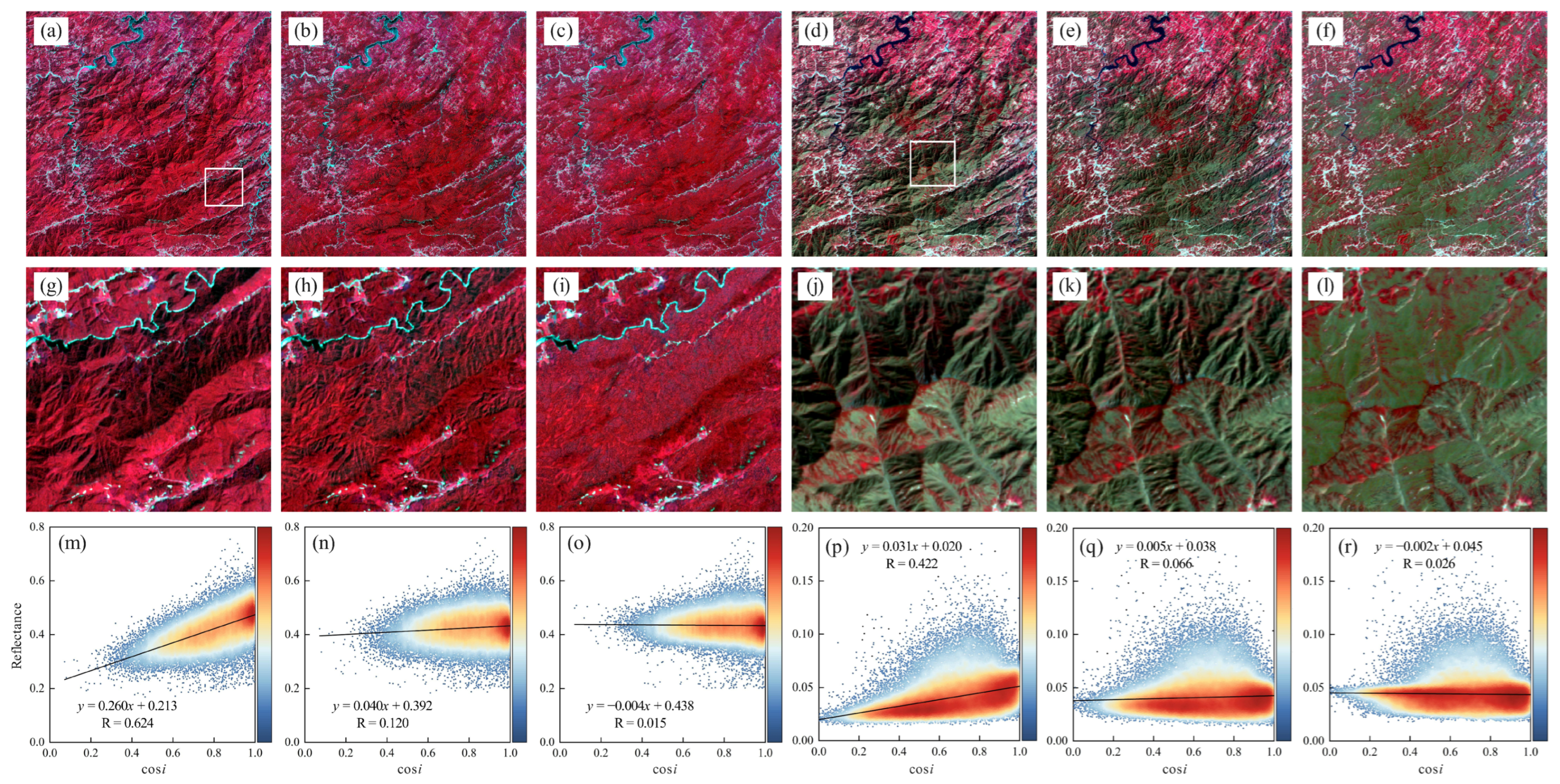
To test the preliminary applicability to other sensors of TSEC+TC, we applied TSEC+SCSC to Sentinel-2 and GF-1 WFV images in the study area. The Sentinel-2 image was acquired on 1 September 2023, and the corrected bands were Blue, Green, Red, and NIR bands at a 10 m resolution. The GF-1 WFV image was acquired on 10 March 2022, at a 16 m resolution, and all bands were involved in the correction. Because the Coastal band is absent from GF-1 WFV imagery, the Blue band was used as a substitute in the SIF calculation. This substitution was adopted because the Blue band has spectral properties relatively close to those of the Coastal band, although the full sensitivity of this replacement requires further evaluation. Figure 14 shows the uncorrected, SCSC-corrected, and TSEC+SCSC-corrected images. The density scatter plots show the correlation between reflectance and illumination conditions before and after correction.

The topographic and shadow effects appeared more prominent in the Sentinel-2 and GF-1 WFV images, particularly the shadow effect, than in the Landsat 8 image. SCSC correction reduced terrain relief and produced flatter images (Figure 14b,e), but many shadow pixels remained visible in the enlarged insets (Figure 14h,k). The TSEC+SCSC-corrected images further reduced the contrast between shadowed and adjacent sunlit areas while maintaining similar false-color hues before and after correction (Figure 14c,f). In the enlarged insets, the corrected shadow pixels showed spectral patterns closer to neighboring pixels than those after SCSC correction alone (Figure 14i,l). The density scatter plots indicate that the correlation between reflectance and cosi was lower after TSEC+SCSC correction than after SCSC correction for both Sentinel-2 and GF-1 WFV images. These results support preliminary applicability of TSEC+TC to the tested 10 m and 16 m scenes. Broader sensor generalization requires tests across additional sensors, regions, and acquisition conditions.

5. Discussion

5.1. Comparison of the TSEC+TC and TC Methods

In Table 4, the RE of PLC reached −19.18% in the corrected results for January, indicating a serious underestimation of the reflectance corrected by this method, which is also confirmed in Figure 8a. Based on the analysis in Figure 6, two factors contributed to the underestimation of the PLC. First, the shadow area was undercorrected, and second, the sunlit area was inversely corrected. The second factor was the inadequate expression of the PLC, which disregarded the effect of scattered radiation. This resulted in ineffective correction under low illumination conditions [30,49]. Combining TSEC with PLC improved the first scenario. This combination explained why the January correction result showed an RE of only −2.80% for TSEC+PLC, as illustrated by the comparison of the corrections for PLC and TSEC+PLC in Figure 6. Similar improvements were observed in SCSC and TSEC+SCSC, where the CV of TSEC+SCSC decreased more than tenfold compared to that of the SCSC method in the January correction results (Table 4). TSEC+SCSC achieved this because it avoided the overcorrection observed in SCSC, resulting in its smoother reflectance curves in Figure 8a.

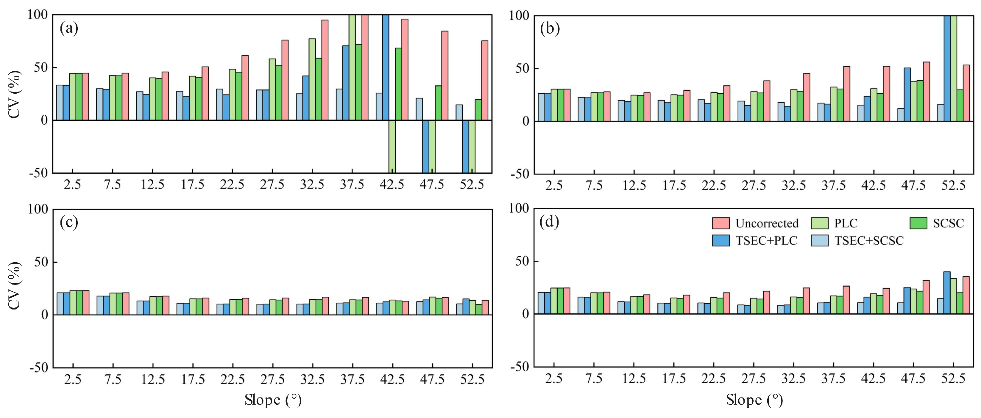
In addition to solar azimuth, solar elevation angle, and aspect, the terrain slope also strongly affects topographic correction performance, particularly in rugged mountainous areas with high terrain relief [12]. To further investigate the influence of slope on the TC (including SCSC and PLC) and TSEC+TC methods (including TSEC+SCSC and TSEC+PLC), we divided the slopes of the study area into 11 grades at intervals of 5° (because there were very few pixels with slopes greater than 55°, and pixels greater than 55° were treated as 55°). Histograms of the slope and coefficient of variation of reflectance in the NIR band were plotted for forestland before and after correction. The central slope value for each grade was used as the x-axis (Figure 15). Since the land cover type was controlled, the corrected CVs for the same land cover type should theoretically be smaller. Additionally, the CV values for the different slope grades should remain similar. The June and September results aligned with this theory, displaying a lower CV after correction for both the TC and TSEC+TC methods. Nonetheless, the September results indicated a slight increase in the CVs for both the PLC and TSEC+PLC methods in the slope range of 50–55°, which closely matched the CV before correction. The January and March results showed this phenomenon more clearly, with abrupt changes in the CV values occurring for slopes of >30° and >45°, respectively. It should be noted that the solar elevation angles recorded by the images were in the range where abrupt changes occurred. This suggests that pixels where the terrain slope exceeds the solar elevation angle cannot be stabilized for correction, which can be explained by the PLC model expression.

The PLC expression and our results indicate a practical caution: instability becomes more likely when local terrain slope approaches or exceeds the solar elevation angle, particularly when aspect is close to the solar azimuth (Figure 8 and Figure 15). Recent studies likewise report reduced PLC performance under faint illumination and low solar elevation conditions [50,51]. Under these conditions, TSEC+SCSC or explicit quality flags are preferable.

Based on the PLC expression (Equations (20)–(22)), for satellite images, S_view and $S_{\mathit{view}}^t$ values were close to 1 owing to zenithal observation characteristics, whereas the S_sun value was greater than or equal to 1. Therefore, the $S_{\mathit{run}}^t$ term remained the primary determinant of reflectance overcorrection. For example, when the surface aspect was close to the solar azimuth, cos(φ − β) in Equation (22) approached 1. In this case, if the product of tanθ_s and tanθ_z was greater than 1 but close to 1, the $S_{\mathit{run}}^t$ term generated a strongly negative value. This resulted in a negative reflectance, as calculated using Equation (20). This explains the “retraction” of the corrected reflectance curves on the same aspect as the solar azimuth for the dates with lower solar elevation angles in Figure 8a,j. This also explains the abrupt change in the CV of the corrected reflectance in Figure 15a,b for areas with larger slope due to the interaction between the slope and the solar zenith angle in Equation (22).

Because TSEC+PLC uses PLC as its sunlit pixel branch, the limitations of PLC are inherited by TSEC+PLC. This explains why dark pixels remained after TSEC+PLC. The dark pixels in the sunlit area resulted from deficiencies in the PLC. The TSEC did not participate in correcting sunlit areas. Therefore, the performance of TSEC+TC in sunlit area correction depended on the correction performance of the TC model combined with it. Although TSEC+PLC can generally reduce undercorrection in shadow areas, the method may not produce optimal correction results when large terrain relief and low solar elevation angles are present simultaneously.

The TSEC+SCSC method improved the SCSC results, with lower CV values than SCSC for all four dates. The CV of TSEC+SCSC also varied little across slopes and remained low, indicating that TSEC+SCSC remained stable in complex terrain and under low solar elevation angles. In addition, the method showed no obvious overcorrection or undercorrection in the outlier and reflectance analyses (Figure 8 and Figure 13). The benefit of TSEC+PLC is that PLC is a physically based approach that can reproduce vegetation reflectance under suitable illumination conditions. Combining TSEC with PLC may therefore improve reflectance estimation in shadowed parts of complex mountainous areas. However, the slope distribution in the study area and the solar elevation angle during image acquisition should still be considered when applying this approach. A recent global assessment of ten TC models across 10,523 Landsat 8 OLI scenes also showed that model performance varies with solar zenith angle, latitude, land cover, and season [52]. This result further supports selecting the TC branch according to scene conditions.

5.2. Selection and Mask Extent Analysis of ${\mathit{SI}}_{\mathit{TOA}}^{\mathit{ac}}$

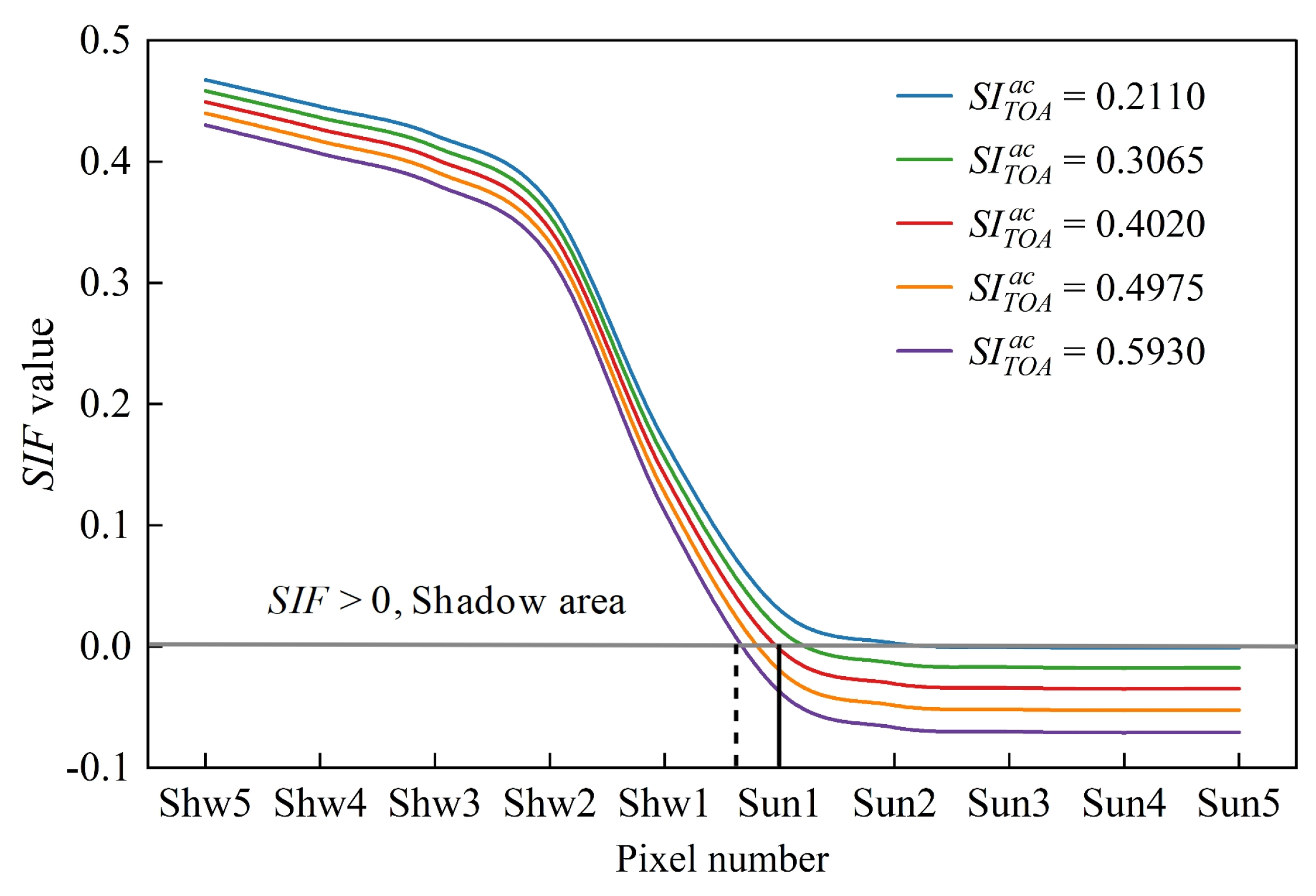
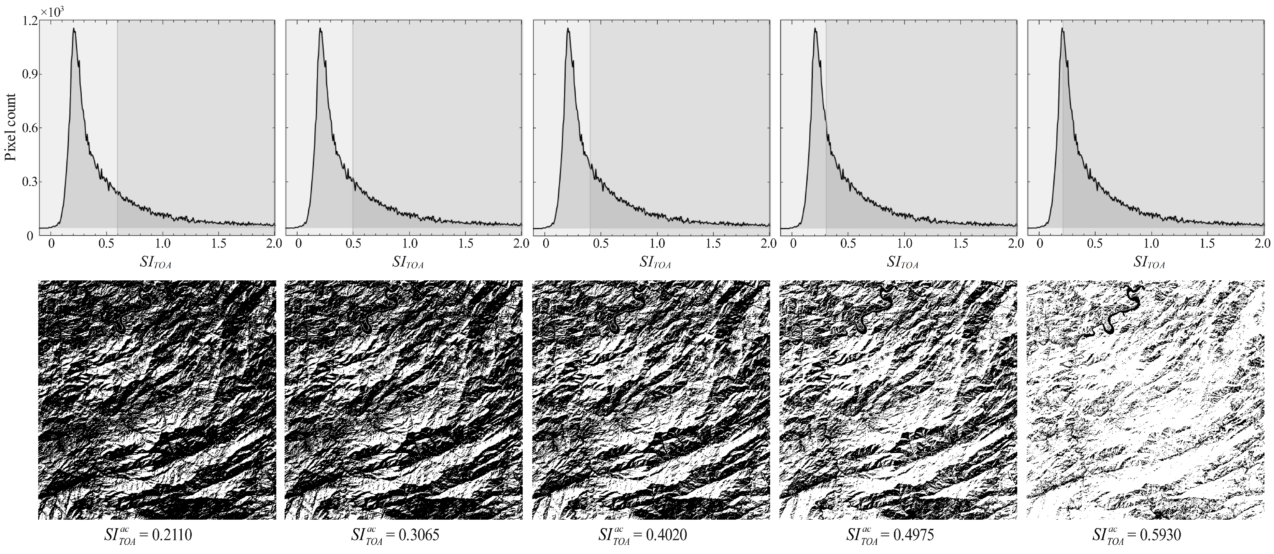
The SI_TOA and ${\mathit{SI}}_{\mathit{TOA}}^{\mathit{ac}}$ in Section 3.1 were used to construct the SIF in Section 3.2. To explain the calculation of ${\mathit{SI}}_{\mathit{TOA}}^{\mathit{ac}}$, the January image is used as an example. The distribution histogram of SI_TOA showed a single peak pattern, and the SI_TOA values at the thresholds calculated by Otsu’s method exceeded the SI_TOA values at the peaks. We divided the interval between the peak and threshold of SI_TOA into four equal sections and calculated the raw SIF values (before application of K_s and restriction to the range 0–1) at each point based on the 50 sets of samples in Section 3.1. The SI_TOA values were obtained at the peak, 1/4 of the interval distance, midpoint, 3/4 of the interval distance, and at the threshold, which corresponded to SI_TOA values of 0.2110, 0.3065, 0.4020, 0.4975, and 0.5930, respectively (Figure 16). The boundary between the shadow and sunlit areas was almost in the middle of the first shadow pixel and the first sunlit pixel when ${\mathit{SI}}_{\mathit{TOA}}^{\mathit{ac}}$ was located at the threshold (black dashed line in Figure 16), indicating that the threshold calculated by Otsu’s method can delineate shadow and sunlit areas. However, when accounting for the penumbra, the boundary between shadow and sunlit areas should be shifted to the first pixel of the sunlit area (solid black line in Figure 16). Under this condition, the selected value for ${\mathit{SI}}_{\mathit{TOA}}^{\mathit{ac}}$ is the midpoint of the interval (${\mathit{SI}}_{\mathit{TOA}}^{\mathit{ac}}$ = 0.4020). Figure A2 shows clear differences in shadow extent among the five candidates. An overly broad mask can apply the shadow branch to sunlit pixels, while an overly narrow mask can leave penumbral or shadow pixels in the TC branch; these cases can produce local overcorrection or undercorrection near the boundary. Our calculations for the 10 scenes indicate that ${\mathit{SI}}_{\mathit{TOA}}^{\mathit{ac}}$ is typically situated near the middle of the peak and threshold of SI_TOA. The midpoint was therefore adopted as a heuristic operational threshold for the present workflow. The effects of threshold selection on R², CV, and OA remain to be quantified and will be examined in future work.

5.3. Difference Between SI_C-G and SI_B-G

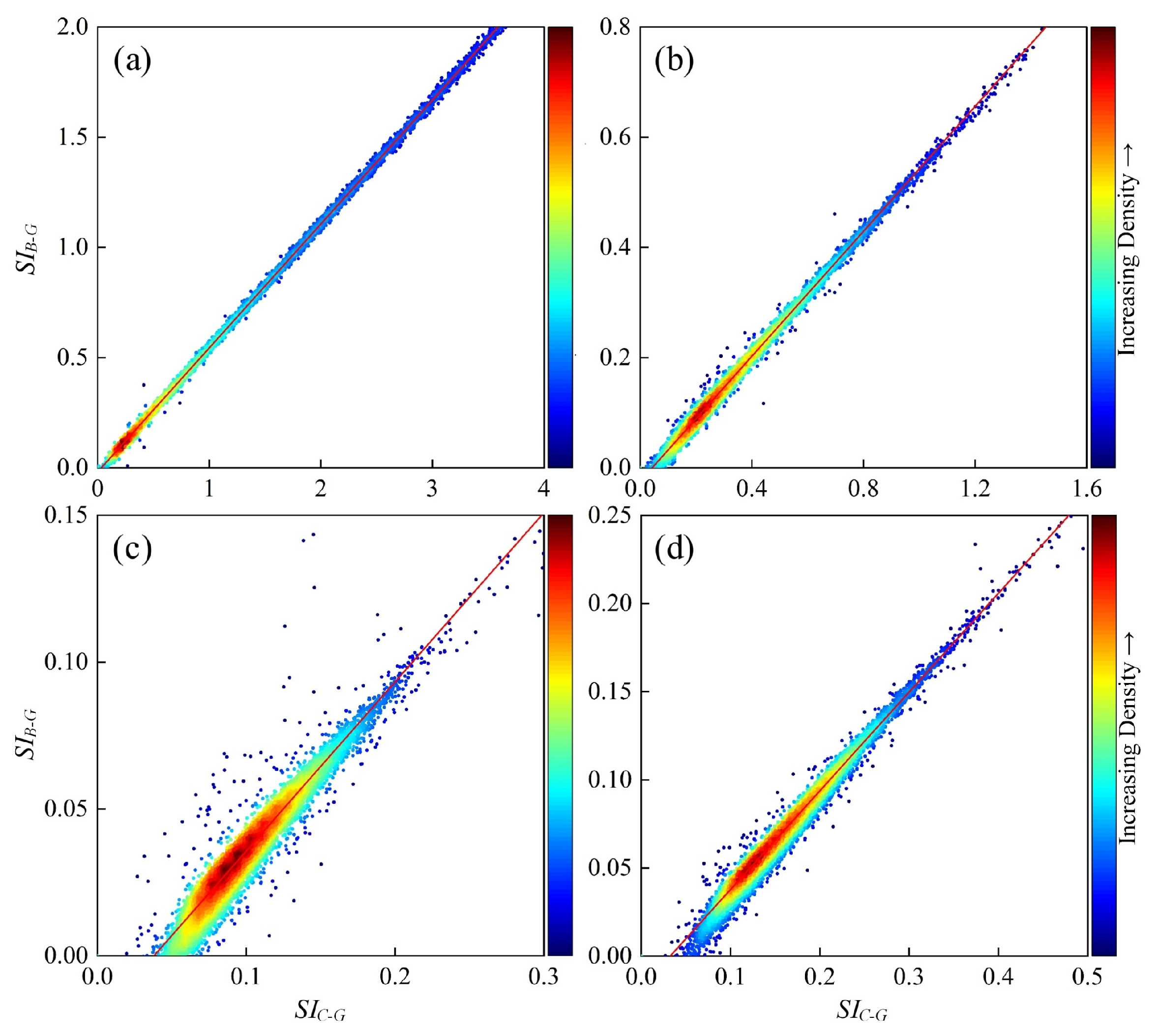
The TSEC model constructed SIF using the Coastal, Green, and NIR bands. The Coastal band is less commonly used, particularly by sensors that capture high-resolution images [53]. Therefore, we constructed SI_B-G in Section 4.7 with Blue bands instead of Coastal bands and introduced it into the calculation of SIF. To further compare SI_B-G and the original SI (denoted SI_C-G) in the TSEC model, as well as the reliability of SI_B-G, we analyzed the differences between SI_C-G and SI_B-G, as shown in Figure 17. The density scatter plot and fitting results showed a strong linear relationship between SI_C-G and SI_B-G and coefficients of determination exceeding 0.9 for all four dates. The scatter density kernel was nearly centered on the fitted line, and the density points exhibited a symmetric distribution, especially in January and March. However, the SI_B-G values for June and September shifted towards SI_C-G. The original images show that vegetation cover was higher in the images from these two dates than in January and March (Figure 1). This suggests that SI_B-G might be slightly less sensitive to shadows than SI_C-G in images with higher vegetation cover. However, the visual inspection and correlation analysis between reflectance and cosi (Figure 14) show that this decrease in sensitivity had minimal impact on the correction results.

Although SI_C-G and SI_B-G differ in shadow sensitivity, the more appropriate index for SIF construction remains unclear. Therefore, further research is needed to determine whether SI_B-G can replace SI_C-G entirely.

5.4. Applicability, Robustness, Limitations, and Future Work

The implementation of TSEC+TC requires a multispectral image, a coregistered DEM, and the corresponding solar and view geometry, with BAF fitted separately for each date and band. The reliability of the correction depends on the information retained in the original observation. In extremely deep shadow, the recorded signal can approach the sensor noise floor, increasing the uncertainty of the corrected reflectance. Such pixels therefore require explicit quality control.

Two BAF estimation strategies are available within the TSEC-derived correction framework. The original strategy [38] uses homogeneous samples, which limits land cover variability but requires sample selection and anchors BAF to the selected cover. The scene level strategy used here estimates BAF automatically from all detected shadow pixels for each acquisition date and spectral band. VIF constrains compensation using vegetation information and may partly moderate variability among vegetated surfaces, but it does not explicitly separate intrinsic reflectance differences among land cover types. Consequently, dominant covers may influence the fitted BAF and leave residual bias for less represented classes, including nonvegetated surfaces. Future work should compare pooled, stratified, and endmember-specific BAF estimation across land cover classes.

The use of a binary shadow mask introduces uncertainty at the transition between sunlit and shadowed areas. SIF partly moderates this effect because it is derived from a spectral shadow index that changes gradually with illumination. Including the penumbra in the shadow branch allows partially illuminated pixels to receive compensation according to shadow intensity, and no obvious boundary discontinuity was observed in the present results. Local discontinuities may still occur where the penumbra is broad or spatially variable, where coarse pixels contain mixed illumination, or where DEM and registration errors affect branch assignment. The sensitivity to DEM quality was not isolated in the present experiments. The midpoint threshold is a heuristic operational choice. Future work will further evaluate its influence on correction performance and explore more robust methods for determining the shadow boundary.

The study area contains cultivated land, shoaly land, and impervious surfaces, with winter phenology increasing the proportion of surfaces showing nonvegetated spectral characteristics. Although visual comparisons suggest reduced brightness variation associated with terrain over these surfaces, quantitative evaluation for individual nonvegetated classes is needed to substantiate this observation. The present evaluation used sunlit reference samples and image statistics, and the Lambertian formulation simplifies surface anisotropy, adjacency effects, and radiative interactions in three dimensions. Future work should examine DEM and threshold sensitivity, incorporate field measurements or radiative transfer simulations where possible, and develop physical bounds for individual bands and surface types.

The classification analysis provides an auxiliary view of how topographic correction affects a downstream thematic product under a common classification setting. The manually delineated training and accuracy assessment sets were not fully mutually exclusive at the pixel level, and performance was summarized using OA under an imbalanced class distribution. Future work will use spatially independent samples and include class-specific accuracy measures to provide a more comprehensive assessment.

6. Conclusions

This study integrated the previously developed TSEC direct light compensation mechanism with representative TC models and proposed a partitioned topographic normalization framework for rugged mountainous terrain. In the proposed TSEC+TC framework, sunlit pixels are normalized using a conventional TC branch, whereas shadowed pixels are estimated using a TSEC-derived compensation branch. The two outputs are combined using a shadow mask to produce a unified horizontal equivalent reflectance image. The method retains a physical basis related to terrain irradiance and requires only one image and a corresponding DEM as the main inputs.

Two representative TC methods (PLC and SCSC) were combined with the TSEC-derived compensation branch to form TSEC+PLC and TSEC+SCSC in this study. Ten Landsat 8 OLI scenes under varying illumination conditions were used to test the performance of TSEC+TC and compare it with selected TC methods. TSEC+TC reduced terrain-related brightness variation and mitigated shadow-induced reflectance distortion compared with TC alone. For images acquired under different illumination conditions, TSEC+TC reduced the correlation between corrected reflectance and illumination conditions, and the corrected reflectance showed high aspect stability, especially for TSEC+SCSC. Compared with TC-only methods, TSEC+TC provided more consistent correction in self shadow and cast shadow areas and better preserved the spectral patterns of shadowed pixels. Under the adopted outlier criterion, TSEC+SCSC produced few outliers and reduced SCSC-induced outliers in shadowed areas. In the auxiliary land cover classification evaluation, TSEC+TC improved classification accuracy, with OA values of 0.64–0.72 after correction, compared with 0.46–0.72 before correction. Tests using Sentinel-2 MSI and GF-1 WFV imagery support preliminary applicability at 10 and 16 m spatial resolutions. Broader sensor applicability requires additional scenes, regions, and sensors.

References

1. Chen, R.; Yin, G.; Zhao, W.; Yan, K.; Wu, S.; Hao, D.; Liu, G. Topographic Correction of Optical Remote Sensing Images in Mountainous Areas: A systematic review. IEEE Geosci. Remote Sens. Mag. 2023, 11, 125–145. [Google Scholar] [CrossRef] [Scilit]
2. Chi, H.; Yan, K.; Yang, K.; Du, S.; Li, H.; Qi, J.; Zhou, W. Evaluation of Topographic Correction Models Based on 3-D Radiative Transfer Simulation. IEEE Geosci. Remote Sens. Lett. 2022, 19, 1–5. [Google Scholar] [CrossRef] [Scilit]
3. Jiang, H.; Jia, K.; Zhao, X.; Wei, X.; Wang, B.; Yao, Y.; Zhang, X.; Jiang, B. Review on the theory, method, and research progress of leaf area index estimation in mountainous areas. Natl. Remote Sens. Bull. 2020, 24, 1433–1449. [Google Scholar] [CrossRef] [Scilit]
4. Rahbek, C.; Borregaard, M.K.; Colwell, R.K.; Dalsgaard, B.; Holt, B.G.; Morueta-Holme, N.; Nogues-Bravo, D.; Whittaker, R.J.; Fjeldså, J. Humboldt’s enigma: What causes global patterns of mountain biodiversity? Science 2019, 365, 1108–1113. [Google Scholar] [CrossRef] [Scilit] [PubMed]
5. Yan, K.; Zou, D.; Yan, G.; Fang, H.; Weiss, M.; Rautiainen, M.; Knyazikhin, Y.; Myneni, R.B. A Bibliometric Visualization Review of the MODIS LAI/FPAR Products from 1995 to 2020. J. Remote Sens. 2021, 2021, 7410921. [Google Scholar] [CrossRef] [Scilit]
6. Yan, K.; Li, H.; Song, W.; Tong, Y.; Hao, D.; Zeng, Y.; Mu, X.; Yan, G.; Fang, Y.; Myneni, R.B.; et al. Extending a Linear Kernel-Driven BRDF Model to Realistically Simulate Reflectance Anisotropy Over Rugged Terrain. IEEE Trans. Geosci. Remote Sens. 2022, 60, 1–16. [Google Scholar] [CrossRef] [Scilit]
7. Wu, Z.; Li, Y.; Xu, X.; Fan, H. Topographic effects amplify forest disturbances detected by yearly wide-time-window Landsat time series. GIScience Remote Sens. 2023, 60, 2222627. [Google Scholar] [CrossRef] [Scilit]
8. Jin, H.; Li, A.; Xu, W.; Xiao, Z.; Jiang, J.; Xue, H. Evaluation of topographic effects on multiscale leaf area index estimation using remotely sensed observations from multiple sensors. ISPRS J. Photogramm. Remote Sens. 2019, 154, 176–188. [Google Scholar] [CrossRef] [Scilit]
9. Van Den Hoek, J.; Smith, A.; Hurni, K.; Saksena, S.; Fox, J. Shedding New Light on Mountainous Forest Growth: A Cross-Scale Evaluation of the Effects of Topographic Illumination Correction on 25 Years of Forest Cover Change across Nepal. Remote Sens. 2021, 13, 2131. [Google Scholar] [CrossRef] [Scilit]
10. Wen, J.; Liu, Q.; Xiao, Q.; Liu, Q.; You, D.; Hao, D.; Wu, S.; Lin, X. Characterizing Land Surface Anisotropic Reflectance over Rugged Terrain: A Review of Concepts and Recent Developments. Remote Sens. 2018, 10, 370. [Google Scholar] [CrossRef] [Scilit]
11. Fan, Y.; Koukal, T.; Weisberg, P.J. A sun–crown–sensor model and adapted C-correction logic for topographic correction of high resolution forest imagery. ISPRS J. Photogramm. Remote Sens. 2014, 96, 94–105. [Google Scholar] [CrossRef] [Scilit]
12. Gao, M.; Gong, H.; Zhao, W.; Chen, B.; Chen, Z.; Shi, M. An improved topographic correction model based on Minnaert. GIScience Remote Sens. 2015, 53, 247–264. [Google Scholar] [CrossRef] [Scilit]
13. Chen, R.; Yin, G.; Liu, G.; Yang, Y.; Wang, C.; Xie, Q.; Zhao, W.; Verger, A. Correction of illumination effects on seasonal divergent NIRv photosynthetic phenology. Agric. For. Meteorol. 2023, 339, 109542. [Google Scholar] [CrossRef] [Scilit]
14. Bishop, M.P.; Colby, J.D. Topographic Normalization of Multispectral Satellite Imagery. In Encyclopedia of Snow, Ice and Glaciers; Encyclopedia of Earth Sciences Series; Springer: Dordrecht, The Netherlands, 2011; pp. 1187–1196. [Google Scholar]
15. Bishop, M.P.; Young, B.W.; Colby, J.D. Surface spectral irradiance and irradiance partitioning in a complex mountain environment: Understanding location-dependent topographic effects in satellite imagery. Geocarto Int. 2023, 38, 2264275. [Google Scholar] [CrossRef] [Scilit]
16. Sola, I.; Gonzalez-Audicana, M.; Alvarez-Mozos, J.; Torres, J.L. Synthetic Images for Evaluating Topographic Correction Algorithms. IEEE Trans. Geosci. Remote Sens. 2014, 52, 1799–1810. [Google Scholar] [CrossRef]
17. Chu, Q.; Yan, G.; Qi, J.; Mu, X.; Li, L.; Tong, Y.; Zhou, Y.; Liu, Y.; Xie, D.; Wild, M. Quantitative Analysis of Terrain Reflected Solar Radiation in Snow-Covered Mountains: A Case Study in Southeastern Tibetan Plateau. J. Geophys. Res. Atmos. 2021, 126, e2020JD034294. [Google Scholar] [CrossRef] [Scilit]
18. Makarau, A.; Richter, R.; Muller, R.; Reinartz, P. Adaptive Shadow Detection Using a Blackbody Radiator Model. IEEE Trans. Geosci. Remote Sens. 2011, 49, 2049–2059. [Google Scholar] [CrossRef]
19. Richter, R.; Müller, A. De-shadowing of satellite/airborne imagery. Int. J. Remote Sens. 2007, 26, 3137–3148. [Google Scholar] [CrossRef] [Scilit]
20. Sandmeier, S.; Itten, K.I. A physically-based model to correct atmospheric and illumination effects in optical satellite data of rugged terrain. IEEE Trans. Geosci. Remote Sens. 1997, 35, 708–717. [Google Scholar] [CrossRef] [Scilit]
21. Bishop, M.P.; Young, B.W.; Colby, J.D. Numerical Modeling and Parameter Sensitivity Analysis for Understanding Scale-Dependent Topographic Effects Governing Anisotropic Reflectance Correction of Satellite Imagery. Remote Sens. 2022, 14, 5339. [Google Scholar] [CrossRef] [Scilit]
22. Shepherd, J.D.; Dymond, J.R. Correcting satellite imagery for the variance of reflectance and illumination with topography. Int. J. Remote Sens. 2010, 24, 3503–3514. [Google Scholar] [CrossRef] [Scilit]
23. Alavipanah, S.K.; Karimi Firozjaei, M.; Sedighi, A.; Fathololoumi, S.; Zare Naghadehi, S.; Saleh, S.; Naghdizadegan, M.; Gomeh, Z.; Arsanjani, J.J.; Makki, M.; et al. The Shadow Effect on Surface Biophysical Variables Derived from Remote Sensing: A Review. Land 2022, 11, 2025. [Google Scholar] [CrossRef] [Scilit]
24. Balthazar, V.; Vanacker, V.; Lambin, E.F. Evaluation and parameterization of ATCOR3 topographic correction method for forest cover mapping in mountain areas. Int. J. Appl. Earth Obs. Geoinf. 2012, 18, 436–450. [Google Scholar] [CrossRef] [Scilit]
25. Lin, X.; Wen, J.; Wu, S.; Hao, D.; Xiao, Q.; Liu, Q. Advances in topographic correction methods for optical remote sensing imageries. Natl. Remote Sens. Bull. 2020, 24, 958–974. [Google Scholar] [CrossRef] [Scilit]
26. Sola, I.; González-Audícana, M.; Álvarez-Mozos, J. Multi-criteria evaluation of topographic correction methods. Remote Sens. Environ. 2016, 184, 247–262. [Google Scholar] [CrossRef] [Scilit]
27. Teillet, P.M.; Guindon, B.; Goodenough, D.G. On the Slope-Aspect Correction of Multispectral Scanner Data. Can. J. Remote Sens. 2014, 8, 84–106. [Google Scholar] [CrossRef] [Scilit]
28. Gao, Y.; Zhang, W. A simple empirical topographic correction method for ETM+ imagery. Int. J. Remote Sens. 2009, 30, 2259–2275. [Google Scholar] [CrossRef] [Scilit]
29. Gu, D.; Gillespie, A. Topographic Normalization of Landsat TM Images of Forest Based on Subpixel Sun–Canopy–Sensor Geometry. Remote Sens. Environ. 1998, 64, 166–175. [Google Scholar] [CrossRef] [Scilit]
30. Yin, G.; Li, A.; Wu, S.; Fan, W.; Zeng, Y.; Yan, K.; Xu, B.; Li, J.; Liu, Q. PLC: A simple and semi-physical topographic correction method for vegetation canopies based on path length correction. Remote Sens. Environ. 2018, 215, 184–198. [Google Scholar] [CrossRef] [Scilit]
31. Proy, C.; Tanre, D.; Deschamps, P. Evaluation of topographic effects in remotely sensed data. Remote Sens. Environ. 1989, 30, 21–32. [Google Scholar] [CrossRef] [Scilit]
32. Soenen, S.A.; Peddle, D.R.; Coburn, C.A. SCS+C: A modified Sun-canopy-sensor topographic correction in forested terrain. IEEE Trans. Geosci. Remote Sens. 2005, 43, 2148–2159. [Google Scholar] [CrossRef] [Scilit]
33. Smith, J.A.; Lin, T.L.; Ranson, K.J. The Lambertian Assumption and Landsat Data. Photogramm. Eng. Remote Sens. 1980, 46, 1183–1189. [Google Scholar]
34. Ge, H.; Lu, D.; He, S.; Xu, A.; Zhou, G.; Du, H. Pixel-based Minnaert Correction Method for Reducing Topographic Effects on a Landsat 7 ETM+ Image. Photogramm. Eng. Remote Sens. 2008, 74, 1343–1350. [Google Scholar] [CrossRef] [Scilit]
35. Jiang, H.; Wang, S.; Cao, X.; Yang, C.; Zhang, Z.; Wang, X. A shadow- eliminated vegetation index (SEVI) for removal of self and cast shadow effects on vegetation in rugged terrains. Int. J. Digit. Earth 2018, 12, 1013–1029. [Google Scholar] [CrossRef] [Scilit]
36. Yang, X.; Zuo, X.; Xie, W.; Li, Y.; Guo, S.; Zhang, H. A Correction Method of NDVI Topographic Shadow Effect for Rugged Terrain. IEEE J. Sel. Top. Appl. Earth Obs. Remote Sens. 2022, 15, 8456–8472. [Google Scholar] [CrossRef] [Scilit]
37. Zhao, W.; Li, X.; Wang, W.; Wen, F.; Yin, G. DSRC: An Improved Topographic Correction Method for Optical Remote-Sensing Observations Based on Surface Downwelling Shortwave Radiation. IEEE Trans. Geosci. Remote Sens. 2022, 60, 1–15. [Google Scholar] [CrossRef] [Scilit]
38. Yang, X.; Xie, W.; Zuo, X.; Guo, S.; Zhu, D.; Li, Y.; Li, J.; Luo, Y. A Topographic Shadow Effect Correction (TSEC) Method for Correcting Surface Reflectance of Optical Remote Sensing Images in Rugged Terrain. Remote Sens. 2026, 18, 642. [Google Scholar] [CrossRef] [Scilit]
39. Tachikawa, T.; Hato, M.; Kaku, M.; Iwasaki, A. Characteristics of ASTER GDEM version 2. In Proceedings of the 2011 IEEE International Geoscience and Remote Sensing Symposium, Vancouver, BC, Canada, 24–29 July 2011; pp. 3657–3660. [Google Scholar]
40. Li, H.; Xu, L.; Shen, H.; Zhang, L. A general variational framework considering cast shadows for the topographic correction of remote sensing imagery. ISPRS J. Photogramm. Remote Sens. 2016, 117, 161–171. [Google Scholar] [CrossRef] [Scilit]
41. Yang, X.; Zuo, X.; Zhu, D.; Xie, W.; Li, Y.; Guo, S. Multi-criteria evaluation of the shadow index performance of Landsat 8 OLI images. Int. J. Remote Sens. 2022, 43, 5125–5144. [Google Scholar] [CrossRef] [Scilit]
42. Sun, G.; Huang, H.; Weng, Q.; Zhang, A.; Jia, X.; Ren, J.; Sun, L.; Chen, X. Combinational shadow index for building shadow extraction in urban areas from Sentinel-2A MSI imagery. Int. J. Appl. Earth Obs. Geoinf. 2019, 78, 53–65. [Google Scholar] [CrossRef] [Scilit]
43. Otsu, N. A Threshold Selection Method from Gray-Level Histograms. IEEE Trans. Syst. Man Cybern. 1979, 9, 62–66. [Google Scholar] [CrossRef] [Scilit]
44. Arévalo, V.; González, J.; Ambrosio, G. Shadow detection in colour high-resolution satellite images. Int. J. Remote Sens. 2008, 29, 1945–1963. [Google Scholar] [CrossRef] [Scilit]
45. Shahtahmassebi, A.; Yang, N.; Wang, K.; Moore, N.; Shen, Z. Review of shadow detection and de-shadowing methods in remote sensing. Chin. Geogr. Sci. 2013, 23, 403–420. [Google Scholar] [CrossRef] [Scilit]
46. Cameron, M.; Kumar, L. Diffuse Skylight as a Surrogate for Shadow Detection in High-Resolution Imagery Acquired Under Clear Sky Conditions. Remote Sens. 2018, 10, 1185. [Google Scholar] [CrossRef] [Scilit]
47. Xue, L.; Yang, S.; Ma, J.; Jia, X.; Yan, R. Automatic expansion extraction algorithm of remote sensing images. Remote Sens. Land Resour. 2019, 31, 42–48. [Google Scholar]
48. Yin, G.; Li, J.; Xu, B.; Zeng, Y.; Wu, S.; Yan, K.; Verger, A.; Liu, G. PLC-C: An Integrated Method for Sentinel-2 Topographic and Angular Normalization. IEEE Geosci. Remote Sens. Lett. 2021, 18, 1446–1450. [Google Scholar] [CrossRef] [Scilit]
49. Yin, G.; Ma, L.; Zhao, W.; Zeng, Y.; Xu, B.; Wu, S. Topographic Correction for Landsat 8 OLI Vegetation Reflectances Through Path Length Correction: A Comparison Between Explicit and Implicit Methods. IEEE Trans. Geosci. Remote Sens. 2020, 58, 8477–8489. [Google Scholar] [CrossRef] [Scilit]
50. Varade, D.; Shen, X.; He, Y.; Chen, L.; Liu, S.; Wu, Z.; Song, S.; Deng, L.; Du, X. SCSCTS: An improved SCS+C topographic correction model with shadow compensation for mountainous regions. PLoS ONE 2026, 21, e0347784. [Google Scholar] [CrossRef] [Scilit] [PubMed]
51. Yu, W.; Huang, H.; Liu, Q.; Wang, J. Integrating physical model and image simulations to correct topographic effects on surface reflectance. ISPRS J. Photogramm. Remote Sens. 2024, 211, 356–371. [Google Scholar] [CrossRef] [Scilit]
52. Geng, J.; Wang, Y.; Roujean, J.-L.; Li, W.; Ma, Y.; Chen, R.; Ding, A.; Jiang, H.; Xu, K.; Gao, F.; et al. Global Adaptability Assessment of Ten Common Topographic Correction Models for Landsat 8 OLI Images. IEEE Trans. Geosci. Remote Sens. 2025, 63, 1–17. [Google Scholar] [CrossRef] [Scilit]
53. Jiang, H.; Chen, A.; Wu, Y.; Zhang, C.; Chi, Z.; Li, M.; Wang, X. Vegetation Monitoring for Mountainous Regions Using a New Integrated Topographic Correction (ITC) of the SCS + C Correction and the Shadow-Eliminated Vegetation Index. Remote Sens. 2022, 14, 3073. [Google Scholar] [CrossRef] [Scilit]
Figure 1. Uncorrected Landsat 8 OLI images of the study area (RGB color space corresponding to band 654).
Remotesensing 18 02719 g001
Figure 2. Schematic of the threshold offset used to include the penumbra. Values inside the boxes are SITOA values, and values between adjacent pixels are vi. The green box marks the boundary pixel reassigned from sunlit to shadow. The ellipses indicate omitted intermediate pixels.
Remotesensing 18 02719 g002
Figure 3. Workflow of the TSEC+TC method and its required inputs.
Remotesensing 18 02719 g003
Figure 4. Landsat 8 OLI images after TSEC+PLC (false color: RGB = Bands 6, 5, and 4). The white box identifies the subregion enlarged in Figure 6.
Remotesensing 18 02719 g004
Figure 5. Landsat 8 OLI images after TSEC+SCSC correction (false color: RGB = Bands 6, 5, and 4).
Remotesensing 18 02719 g005
Figure 6. Images of the subregion marked in Figure 4 before and after correction. The four rows represent January, March, June, and September; the seven columns represent uncorrected, MIN, SE, PLC, TSEC+PLC, SCSC, and TSEC+SCSC, respectively.
Remotesensing 18 02719 g006
Figure 7. Scatter plots of the Red band reflectance with cosi before and after correction for each month. (aj) represent Jan, Feb, Mar, Apr, May, Jun, Aug, Sept, Oct, and Nov, respectively.
Remotesensing 18 02719 g007
Figure 8. Reflectance values before and after correction of the SWIR1 band for different aspects. (aj) represent January, February, March, April, May, June, August, September, October, and November, respectively.
Remotesensing 18 02719 g008
Figure 9. SWIR1 band reflectance distribution in the sunlit, self shadow, and cast shadow areas before and after correction. (ag) represent uncorrected, MIN, SE, PLC, TSEC+PLC, SCSC, and TSEC+SCSC, respectively.
Remotesensing 18 02719 g009
Figure 10. Mapping of classification results. (a) indicates the land cover types; (bh) represent the uncorrected, MIN, SE, PLC, TSEC+PLC, SCSC, and TSEC+SCSC classification results for September; (io) denote the uncorrected, MIN, SE, PLC, TSEC+PLC, SCSC, and TSEC+SCSC classification results for January.
Remotesensing 18 02719 g010
Figure 11. Classification accuracy before and after image correction.
Remotesensing 18 02719 g011
Figure 12. Comparison between the reflectance before and after correction by PLC, TSEC+PLC, SCSC, and TSEC+SCSC with reference proxy values (solid lines indicate the mean and colored areas indicate ±1 standard deviation). (ae) are forestland and (fj) are grassland.
Remotesensing 18 02719 g012
Figure 13. Statistics of outliers after correction by different methods.
Remotesensing 18 02719 g013
Figure 14. Correction results and correlation analysis for Sentinel-2 MSI and GF-1 WFV images. (ac) show the uncorrected, SCSC-corrected, and TSEC+SCSC-corrected Sentinel-2 false-color images, respectively; (df) show the corresponding GF-1 WFV false-color images. (gi) are enlarged views of the white boxed area in (a) for Sentinel-2, and (jl) are enlarged views of the white boxed area in (d) for GF-1 WFV. (mo) show the density scatter plots between NIR-band reflectance and cosi for Sentinel-2, and (pr) show the density scatter plots between Red-band reflectance and cosi for GF-1 WFV. For each sensor, the three columns represent the uncorrected, SCSC-corrected, and TSEC+SCSC-corrected results.
Remotesensing 18 02719 g014
Figure 15. Variation in CV of NIR band reflectance with slope for four dates. (ad) January, March, June, and September, respectively.
Remotesensing 18 02719 g015
Figure 16. Pixelwise SIF transition from shadow to sunlit areas for alternative SI TOA ac values. The dashed line marks the Otsu boundary, and the solid line marks the first sunlit pixel included after accounting for penumbra.
Remotesensing 18 02719 g016
Figure 17. Density scatter plots between SIC-G and SIB-G for (a) January, (b) March, (c) June, and (d) September.
Remotesensing 18 02719 g017