Physics-Aware Deep Learning Reconstructs Ground Contamination from Sparse UAV Radiation Measurements over the Fukushima Ukedo Basin Without Field Training

Highlights

What are the main findings?

• A physics-aware U-Net trained entirely on simulation reconstructs ground contamination from sparse UAV aerial radiation measurements without field fine-tuning, achieving ~23% RMSE reduction over IDW and ~15% over ordinary kriging across 25 split × initialisation runs.
• The conventional aerial interpolators IDW and kriging share a structural prediction ceiling near 6000 CPS imposed by the double-blurring of forward-convolved measurements; the physics-aware model surpasses this ceiling.

What are the implications of the main findings?

• The operational value of physics-aware reconstruction is concentrated in high-intensity hotspot recovery: at T = 6000 CPS, U-Net ensemble recovery reaches ~80% while IDW and kriging recovery rates fall to ~0%.
• Operational deployment of physics-aware aerial radiation mapping should use ensemble averaging at inference to control single-model variance, and dedicated spatially independent evaluation with a PSF-matched buffer should accompany any cross-site generalisation claim.

Abstract

Aerial radiation surveys produce sparse trajectories that must be reconstructed into contamination maps. Conventional aerial interpolators—inverse distance weighting (IDW) and ordinary kriging—treat observations as local ground samples, ignoring that each measurement integrates radiation over an extended footprint A(x, y) = (C * K)(x, y). The resulting double-blurring imposes a second smoothing on already-convolved values, causing systematic underprediction regardless of measurement density. We cast reconstruction as inverse deconvolution. A physics-aware encoder–decoder receives five channels (sparse measurements, IDW baseline, land–water scalar prior, measurement mask, water mask) and learns to invert K under a forward-consistency loss. The network is pretrained on synthetic data and deployed without fine-tuning. At a 50% random within-system holdout over the 2213-point Ukedo benchmark trajectory, 25 runs achieve a mean root-mean-square error (RMSE) of 705.4 ± 102.8 counts per second (CPS) versus 916.8 ± 34.2 (IDW) and 832.4 ± 31.3 (Kriging), with directional improvement over IDW in 25/25 runs. In a three-model ensemble diagnostic, among held-out points exceeding T = 6000 CPS (n = 64 at split seed 10, near the IDW ceiling), the U-Net recovers approximately 80% while IDW and kriging both fall to approximately 0%. The operational value lies in high-intensity hotspot recovery. These gains apply to dense-trajectory, within-coverage reconstruction; under large-gap extrapolation beyond the observed trajectory, the advantage over conventional interpolation is drastically reduced, and spatially independent validation remains an open challenge.

1. Introduction

1.1. Airborne Radiation Mapping as an Inverse Problem

Aerial radiation surveys have become a standard tool for characterising the spatial distribution of radioactive contamination following nuclear accidents. Unmanned aerial vehicles and manned helicopters equipped with gamma-ray detectors can traverse large areas rapidly, operate above terrain that is inaccessible to ground teams, and produce georeferenced count-rate trajectories at densities impractical to achieve by surface surveying alone [1,2,3,4]. These properties make airborne platforms valuable for rapid spatial assessment in the aftermath of a radiological event [5,6]. A persistent challenge is that the resulting trajectory data are sparse relative to the continuous ground contamination field they are intended to characterise, and recovering that field from the available observations is not straightforward.

The difficulty arises because an aerial gamma-ray measurement does not sample the ground contamination field locally. At flight altitude h, a detector integrates radiation contributions from a broad surrounding area, with each ground source attenuated by geometric spreading and air absorption. Denoting the ground contamination field as C(x, y) and the resulting aerial measurement field as A(x, y), the forward measurement process takes the form

A(x, y) = (C * K)(x, y)

(1)

where K is a spatially extended physics kernel encoding the inverse-square geometric factor and the effective air attenuation coefficient [7,8], and * denotes two-dimensional convolution. Each aerial observation is therefore a spatially blurred, weighted composite of ground-source values over an extended footprint rather than a point sample of C at the measurement location. Reconstructing C from sparse aerial observations is consequently an inverse problem—not an interpolation problem.

This distinction has direct methodological consequences. Conventional interpolation of aerial observations preserves the forward-convolution blurring: the reconstructed surface inherits the spatial spreading encoded in K regardless of how densely the trajectory is sampled, because the blurring arises from measurement physics, not data quantity. Resolving it requires inverting the forward operator—recovering C(x, y) from sparse observations of A(x, y)—which is the central axis of the present study.

1.2. The Ukedo Benchmark and Its Quantitative Assessment Gap

Kim et al. [9] conducted simultaneous aerial radiation surveys of the Fukushima Ukedo River basin in November 2015, deploying two independent monitoring systems—KINS and JAEA—along identical flight paths within 10 km of the Fukushima Dai-ichi Nuclear Power Station. The two systems produced contamination maps that were qualitatively consistent and exhibited a strong inter-system linear correlation, providing independent corroboration of the spatial contamination pattern over the survey area [9]. This cross-validated measurement record constitutes the empirical basis of the present study.

Despite this agreement, Kim et al. [9] were unable to complete a quantitative comparison of the two maps. Two obstacles prevented it. First, the authors identified the absence of a principled similarity assessment method as an open problem, noting that “there is a need for a method capable of assessing how similar these outcomes are” [9]. Second, the two systems projected their measurements onto distinct spatial grids, making direct pixel-level map-to-map comparison infeasible. Taken together, these constraints left the Ukedo dataset without a quantitative axis for evaluating the correspondence between independently reconstructed contamination maps.

The present study uses the KINS trajectory data from Kim et al. [9] and establishes a within-system held-out validation axis—withholding a subset of trajectory measurements and evaluating aerial-domain prediction accuracy—rather than attempting the inter-system comparison that could not be completed in the original survey.

1.3. Aerial Interpolation: The Current Practice and Its Structural Limitation

Sparse aerial radiation surveys produce georeferenced count-rate trajectories that must be extrapolated to unsampled locations before a contamination map can be constructed. Spatial interpolation fills this gap by estimating field values at unobserved points from nearby measurements. Inverse distance weighting (IDW), which assigns each unobserved location a weighted average of neighbouring observations with weights decaying as a function of distance, is among the most widely used approaches for this purpose. It requires no training data, scales readily to arbitrary survey geometries, and has a long operational record in airborne radiation mapping. Ordinary kriging, a geostatistical estimator that derives weights from a fitted spatial covariance model rather than from a fixed distance kernel, is similarly common in geophysical applications. Conventional aerial interpolation methods such as IDW and ordinary kriging together represent the current practice for gap-filling sparse airborne measurement trajectories.

The structural limitation of this approach follows directly from the inverse-problem framing established in Section 1.1. Each aerial measurement is not a local sample of the ground contamination field C(x, y); it is a spatially blurred composite of ground-source contributions governed by A(x, y) = (C * K)(x, y), where K is the physics kernel encoding geometric spreading and air attenuation. Conventional interpolators receive a sparse set of these already-convolved values {A_i} and produce a spatially dense estimate by spatial averaging, which is itself a smoothing operation regardless of whether the weights are derived from inverse-distance powers (IDW) or from a fitted variogram (kriging). This compound operation is termed double-blurring: the aerial signal is already a spatially convolved version of the ground source, and conventional aerial interpolation imposes a second, interpolation-induced smoothing on top of it.

A critical consequence of double-blurring is that it cannot be resolved by increasing aerial measurement density. Additional observations reduce the interpolation-induced component of the error, but the forward-convolution component is a physical property of the measurement process and is present in every aerial sample regardless of how many are collected. In the limit of dense coverage, IDW and kriging both converge to a faithful estimate of the aerial field A(x, y) = (C * K)(x, y)—not of the ground source C(x, y). This limitation affects the forward-convolution component, which is irreducible: denser sampling reduces interpolation noise but cannot invert the measurement kernel. Section 3.1 provides empirical evidence of this prediction in the Ukedo field data; Section 3.5.1 demonstrates that the limitation is shared by both IDW and kriging.

1.4. Simulation-Pretrained Deep Learning for Inverse Deconvolution

Deep learning has been applied successfully to inverse problems across remote sensing and medical imaging [10,11], where the goal is to recover an unobserved signal from indirect or degraded observations. Encoder–decoder architectures such as U-Net [12] are particularly well suited to this class of problem, learning direct mappings from observation space to reconstruction space through convolutional feature extraction and skip connections that preserve spatial detail. Neural networks have recently been applied to aerial radiation field estimation and spatial-dose reconstruction from airborne measurements [13,14]. A recurring practical constraint is that training such models requires ground-truth fields that are spatially dense—a requirement that cannot be met in field radiation surveys, where only the sparse aerial trajectory is available.

When dense field ground truth is unavailable, a physics-based forward model provides an alternative training source. The forward measurement model established in Section 1.1—A(x, y) = (C * K)(x, y)—directly specifies the relationship between any hypothetical ground source C and the aerial measurements A it would produce. Simulating a population of plausible ground-source configurations and projecting each through the forward kernel generates paired training examples without field measurement [10]. A model pretrained on this synthetic corpus can then be applied directly to real aerial trajectories without any field-based fine-tuning—a zero-shot sim-to-real transfer strategy. The fidelity of the transfer rests on the forward kernel being the same physical process in both the simulation and the field measurement. The present study differs from prior neural approaches to aerial radiation mapping in three respects. Sasaki et al. [13] trained neural networks on measured dose-rate data to visualise dose-rate distributions, and Sun et al. [14] optimised long-term monitoring configurations from observed air-dose-rate records; both use field measurements as training data. In contrast, the model developed here (i) is trained exclusively on synthetic data generated by an explicit forward measurement model, requiring no field training data—whereas recent deep learning applications to UAV-borne gamma-ray data have focused on image enhancement such as super-resolution of spectrum images [15] rather than physically constrained inversion; (ii) cast reconstruction as inverse deconvolution of the measurement kernel K rather than regression on observed dose rates; and (iii) enforcing forward consistency between the inferred ground field and the observed aerial signal during training. Relative to general deep inverse-problem frameworks in imaging [10,11,16], the contribution is the domain instantiation: a radiation-specific forward kernel, terrain priors, and a validation protocol designed for surveys lacking dense ground truth.

The model developed in this study is physics-aware in three respects beyond the training data source, instantiating mechanisms that the physics-informed machine learning literature has documented as broadly effective for scientific inverse problems [17,18,19]. First, the training loss includes a forward-consistency term: the inferred ground field is re-projected through K and compared against the observed aerial values, enforcing physical coherence between the reconstruction and the measurements. Second, the land–water context is encoded explicitly through two complementary input channels—a continuous land–water scalar prior and a discrete binary water mask—capturing both the expected surface dose-rate magnitude over land relative to flowing water and the precise spatial location of river pixels [20], reflecting the physical property that surface cesium-137 deposition is substantially reduced in flowing river channels. Third, a non-negativity constraint on the output ensures physically meaningful reconstructions. Together with the sparse aerial measurements, an interpolated initial estimate, and a measurement mask, these components constitute a five-channel sufficient information set for the inverse deconvolution. The resulting model does not merely interpolate; it learns to invert the forward measurement process under physical constraints.

1.5. Contributions

The contributions of this study are four-fold:

• A within-system held-out validation protocol that provides a quantitative axis for evaluating sparse UAV aerial radiation reconstruction in the absence of a dense surface ground truth. The protocol withholds a subset of the aerial trajectory from the reconstruction model and compares aerial-domain predictions against the withheld observations.
• A demonstration of zero-shot sim-to-real transfer: a physics-aware encoder–decoder network pretrained solely on simulated data, without any field-based fine-tuning, reconstructs real UAV measurements over the Fukushima Ukedo basin.
• Robust improvement under random within-system holdout (~23% over IDW and ~15% over ordinary kriging across 5 splits × 5 model initializations, with directional agreement in 25/25 runs), supported by supplementary analyses showing that the gain is concentrated in high-intensity hotspot recovery rather than uniform improvement across the intensity range.
• Quantitative reactivation of the Kim et al. [9] Ukedo benchmark. The original survey identified the absence of a principled reconstruction accuracy metric as an open problem; the within-system held-out protocol introduced here supplies that axis.

The remainder of this paper is organised as follows: Section 2 describes the study area, simulation framework, and network architecture; Section 3 presents the quantitative results; Section 4 discusses the findings and their implications; and Section 5 concludes.

2. Methods

2.1. Study Area and Dataset

Aerial radiation measurements were collected over the Ukedo River basin, located within 10 km of the Fukushima Dai-ichi Nuclear Power Plant, on 3–4 November 2015. The survey area is characterised by a river basin landscape with a pronounced land–water contrast, where the Ukedo River crosses the contaminated zone. The dataset was originally acquired as part of a cross-system comparison study reported by Kim et al. [9], in which two independent aerial radiation monitoring systems—operated by the Korea Institute of Nuclear Safety (KINS) and the Japan Atomic Energy Agency (JAEA)—surveyed the same region along identical flight trajectories. The present study uses the KINS system data only.

Measurements were acquired using a Yamaha RMAX G1 autonomous unmanned helicopter flown at an altitude of 30 m above ground level, with a lateral flight-line spacing of 30 m and a forward speed of approximately 5 km/h. Gamma-ray counts were recorded by a pair of LaBr3(Ce) scintillation detectors (2.0-inch diameter × 2.0-inch height each) mounted on the helicopter platform, as described in Kim et al. [9].

The dataset comprises 2213 georeferenced trajectory points (Figure 1). Each point records four fields: acquisition time (UTC), geographic latitude, geographic longitude, and count rate in counts per second (CPS). The CPS values range from 1809 to 11,184 across the full trajectory. Only the CPS count rate was used in this study; the full gamma-ray spectral channels available in the raw data were not utilised, as the focus of the present work is on spatial reconstruction rather than spectral decomposition.

2.2. Simulation Pretraining

The complete two-phase pretraining and evaluation workflow is summarised in Figure 2. The network was pretrained exclusively on synthetic data generated from a physics-based forward measurement model. The forward model describes how a detector flying at altitude h above a ground-level radiation field produces a measured count rate. For a detector located at horizontal offset (dx, dy) from a point source at ground level, the measured signal follows an inverse-square law with exponential air attenuation:

K(dx, dy) = exp(-mu * d)/(dx^2 + dy^2 + h^2)

(2)

where d = sqrt(dx^2 + dy^2 + h^2) is the straight-line distance from source to detector, mu = 0.007 m^−1 is an effective linear attenuation coefficient for gamma radiation in air [7], and h = 30 m is the nominal flight altitude matching the Kim et al. [9] survey protocol. The full aerial measurement at each detector position (x, y) was modelled as a two-dimensional convolution of the ground-source field g(x’, y’) with the following kernel:

aerial(x, y) = sum over (x’, y’) of g(x’, y’) * K(x − x’, y − y’)

(3)

The kernel was evaluated on a discrete grid with a cell size of approximately 10 m × 10 m, matching the spatial resolution of the rasterised trajectory data described in Section 2.3.

Synthetic ground-source fields were generated by superimposing 5 to 15 randomly placed Gaussian hotspots over a diffuse background level set at 0.3 times the mean hotspot amplitude. To incorporate water-shielding physics, each hotspot intensity was multiplied by (1—water_mask) at the corresponding grid cell, where water_mask is the same binary water-channel map used as input channel 4 (Section 2.3). This reflects the physical behaviour of Cs-137, whose surface deposition is substantially reduced in flowing river channels and is therefore suppressed over river pixels. All ground-source fields were normalised to the range [0, 1] before forward projection.

Aerial measurement fields were obtained by applying the forward convolution to each synthetic ground source. A random sparsity mask was then applied, retaining between 10% and 90% of grid cells as simulated trajectory observations and setting all remaining cells to zero. An IDW baseline was computed from the retained points to serve as the second input channel (Section 2.3). A total of 1000 samples were generated for training and 200 for validation. No real Ukedo trajectory data were used during pretraining; all parameters were drawn from the synthetic distribution at each iteration.

2.3. Physics-Aware Network Architecture

The 2213 georeferenced trajectory points were rasterised onto a discrete 64 × 128 grid (height × width) prior to model input. Geographic coordinates were mapped to grid indices by linear scaling between the observed latitude and longitude extents of the survey; each grid cell represents approximately 10 m × 10 m on the ground, consistent with the kernel resolution described in Section 2.2. Where multiple trajectory points fell within the same cell, their CPS values were averaged. Cells containing at least one observation were treated as measured; all remaining cells were set to zero and identified by a separate mask channel. This rasterisation procedure was applied identically to the physics-aware model and to the IDW baseline, ensuring a fair comparison on the same spatial grid.

The network received a five-channel input tensor of shape 5 × 64 × 128. Channel 0: Sparse aerial measurements (CPS normalised by the per-sample maximum, non-zero only at observed grid cells). Channel 1: IDW baseline (spatially dense interpolation providing a full-field initialisation). Channel 2: Land–water scalar prior (a continuous-valued scalar map taking the value 5.0 on land cells and 3.0 on water cells, encoding the expected relative magnitude of surface dose-rate contributions; this scalar is normalised by 10 before being fed to the network). Channel 3: Measurement mask (binary indicator set to one at observed cells, allowing the network to distinguish a genuinely low measurement from an unobserved cell). Channel 4: Water mask (binary map derived from the Ukedo basin river boundary, providing the discrete spatial location of water pixels and reflecting the physical property that Cs-137 deposition is suppressed in flowing water). Channels 2 and 4 together encode the land–water physical context: the scalar prior provides the expected magnitude of surface dose-rate, while the binary water mask provides precise spatial localisation. This five-channel input constitutes a sufficient information set to resolve the inverse deconvolution in the presence of water shielding and sparsity.

The network followed an encoder–decoder architecture with skip connections [12]. The encoder comprised three double-convolution blocks with group normalisation (8 groups) and ReLU activations, progressively expanding feature maps from 5 to 16, 16 to 32, and 32 to 64 channels, with max-pooling between stages. Group normalisation was chosen over batch normalisation to provide stable normalisation statistics at the batch size of 16 used here, where per-batch mean and variance estimates can be noisy. The decoder mirrored this structure using transposed convolutions, with skip connections concatenating encoder and decoder feature maps at matching spatial resolutions. A final 1 × 1 convolution followed by a Softplus activation produced the output: a single-channel estimated ground-source field of shape 1 × 64 × 128. Softplus was chosen to guarantee non-negative outputs, consistent with the physical constraint that ground contamination counts per second cannot be negative.

The network was trained with a forward-consistent composite loss:

L = L_surface + 2.0 × L_aerial

(4)

L_surface = SmoothL1(G_pred, G_true)

(5)

L_aerial = SmoothL1(G_pred * K, A_true)

(6)

where G_pred is the predicted ground-source field, G_true is the synthetic ground truth, (*) denotes two-dimensional convolution with the physics kernel K from Section 2.2, and A_true is the simulated aerial field. L_surface penalises deviation from the true ground field directly; L_aerial penalises inconsistency between the forward projection of the predicted field and the observed aerial signal, enforcing physical self-consistency. The aerial consistency term was weighted at 2.0 to emphasise agreement in the aerial domain, which is the domain in which held-out validation is conducted.

Five independent training runs were performed using random seeds {42, 123, 2026, 7, 99} applied to model weight initialisation only. The Adam optimiser was used with a learning rate of 1 × 10^−3 and a batch size of 16. Training ran for 30 epochs on 1000 synthetic samples, with 200 held-out synthetic samples used for validation loss monitoring. All computations were performed in PyTorch on an NVIDIA GPU. The complete two-phase workflow is summarised in Algorithm 1, and the full simulation and training configuration in

Table A1. Simulation and training configuration.

Parameter	Value
Grid	64 × 128 cells (~10 m × 10 m)
Observed-data ratio	50% fixed
Split seeds	{10, 20, 30, 40, 50}
Model seeds	{42, 123, 2026, 7, 99}
Training samples	1000
Validation samples	200
Training epochs	30
Learning rate	1 × 10−3
Batch size	16
Loss weights	L = L_surface + 2.0 × L_aerial (SmoothL1)
UAV altitude for kernel	30 m
Air attenuation coefficient	μ = 0.007 m−1

(Appendix A).

Algorithm 1. Two-phase pretraining and zero-shot deployment. ⊙ denotes element-wise masking; * denotes two-dimensional convolution with the physics kernel K.

Phase 1—Pretraining (synthetic data only)

for each of 1000 synthetic samples:

C ← random ground source (Gaussian hotspots; water-suppressed; normalised)

A ← C * K   ▹ forward projection, Equation (3)

M ← random sparsity mask (10–90% observed)

x ← [A⊙M, IDW(A⊙M), S_landwater, M, W]   ▹ 5-channel input

Ĉ ← UNet_θ(x)

L ← SmoothL1(Ĉ, C) + 2.0·SmoothL1(Ĉ * K, A)   ▹ Equations (4)–(6)

update θ (Adam, 30 epochs over the corpus)

freeze θ

Phase 2—Zero-shot deployment (real trajectory, no fine-tuning)

A_obs ← rasterised observed trajectory points (50% split)

x ← [A_obs, IDW(A_obs), S_landwater, M_obs, W]

Ĉ ← UNet_θ(x)   ▹ inferred ground field

 ← Ĉ * K   ▹ forward projection

score  at held-out trajectory coordinates   ▹ RMSE, Equation (7)

2.4. Within-System Held-Out Validation Protocol

No dense surface measurement exists against which a reconstructed ground contamination map can be directly evaluated in this field setting. An alternative is to withhold a portion of the aerial trajectory from the model and assess reconstruction quality by comparing forward-projected aerial predictions at withheld locations against the corresponding measured CPS values. This within-system held-out protocol was adopted because it circumvents the grid-compatibility limitation that prevented Kim et al. [9] from performing a direct map-to-map comparison between the two independently surveyed systems: evaluating at trajectory-point coordinates requires no grid alignment or inter-system calibration.

The 2213 trajectory points were divided into an input portion and a held-out portion at a fixed 50% observed-data ratio. Five independent splits were generated using distinct random seeds ({10, 20, 30, 40, 50}), each randomly assigning half the trajectory points to the input set and the remainder to the held-out evaluation set. Because the split was random at the trajectory-point level rather than spatial blocks, each partition represents an independent draw of the data arrangement. The held-out set comprised 1107 points in every split. For each of the five splits, five physics-aware model initializations were trained using random seeds {42, 123, 2026, 7, 99} applied to network weight initialization only, yielding 25 total training runs in a 5 × 5 hierarchical design. The IDW baseline is deterministic given a fixed input set and was therefore evaluated once per split (5 evaluations in total); observed variability in IDW RMSE across splits reflects differences in partition difficulty rather than estimator noise.

Validation proceeded in three steps: (i) the input set was used to construct both the IDW baseline and the U-Net reconstruction (each yielding a 64 × 128 ground-source field); (ii) each ground-source field was forward-projected through K to produce a predicted aerial field; and (iii) predicted aerial values were sampled at held-out trajectory coordinates and compared point-wise to measured CPS. This places both methods in the same aerial domain, ensuring that performance differences reflect reconstruction quality rather than evaluation geometry.

This protocol addresses the quantitative assessment gap identified in Kim et al. [9], where system outputs could not be placed on a common evaluation axis due to grid incompatibility and inter-system calibration offsets. By restricting evaluation to a single system (KINS) and comparing predictions to held-out observations from the same trajectory, both sources of inter-system ambiguity are avoided. The protocol does not replace inter-system validation; it provides a reproducible within-system quantitative axis that was absent from the original field study. Extension to inter-system comparison is left to future work.

2.5. Evaluation Metrics

Reconstruction performance was quantified primarily by the root-mean-square error (RMSE) of predicted aerial count rates at held-out trajectory points:

RMSE = sqrt(mean((y_true − y_pred)^2))

(7)

where y_true is the measured CPS at a held-out trajectory point and y_pred is the aerial CPS obtained by forward-projecting the reconstructed surface through the physics kernel at the same geographic coordinate. RMSE was selected as the primary metric because it penalises large deviations and is directly interpretable in the units of the original measurement (counts per second, CPS). Evaluation in the aerial domain, rather than at the surface, reflects the absence of dense surface reference measurements in the field, as described in Section 2.4. The full set of evaluation metrics used in this study is summarised in

Table 1. Glossary of evaluation metrics used in the main text.

Metric	Definition	Interpretation
RMSE (CPS)	sqrt(mean((y_true − y_pred)2)) over held-out points	Primary accuracy metric; penalises large deviations; lower is better
MAE (CPS)	mean(|y_true − y_pred|)	Linear-scale complement to RMSE; lower is better
MBE (CPS)	mean(y_pred − y_true)	Directional bias; negative = systematic underprediction; near zero is better
Pearson r/CCC	Linear correlation/concordance correlation at held-out points	CCC additionally penalises systematic offset; higher is better
Recovery rate at T	P(y_pred ≥ T|y_true ≥ T) over held-out points	Operational hotspot detection capability at threshold T; higher is better
Prediction ceiling (CPS)	95th percentile of predictions among points with observed CPS in top decile	Saturation level of a method in the high-intensity regime
Blocked-fold RMSE inflation (CPS)	RMSE(blocked protocol) − RMSE(random holdout), per method	Sensitivity of a method to large-gap extrapolation (Section 3.5.4)

.

Four secondary metrics were computed alongside RMSE. Mean absolute error (MAE) provides a linear-scale complement to RMSE. Lin’s concordance correlation coefficient (CCC) penalises systematic bias in addition to linear correlation, being depressed when predictions are consistently offset from observations. Mean bias error (MBE = mean(y_pred − y_true)) characterises directional tendency; positive values indicate overprediction. Two supplementary metrics—Spearman rank correlation and top-10% hotspot overlap (the fraction of true 90th-percentile locations jointly recovered above the same threshold)—characterise spatial ordering fidelity and hotspot localisation.

The Pearson correlation at held-out points is referred to throughout as the within-system held-out correlation—an intra-system prediction accuracy metric, distinct from the inter-system correlation reported in Kim et al. [9] between two independent detector systems traversing the same path.

All metrics were evaluated at each of the 25 runs in the 5 split × 5 model seed design. For the physics-aware model, results are reported as mean ± standard deviation across all 25 runs. The IDW and ordinary kriging baselines, being deterministic given a partition, yield one value per split; baseline summary statistics are reported as mean ± standard deviation across the five independent splits. Implementation details of the IDW and ordinary kriging baselines (power exponent, neighbour rule, variogram model, range, nugget, software libraries and versions) are provided in Section 3.1.

3. Results

3.1. Linear Interpolation Baselines at 50% Holdout

We compare the physics-aware reconstruction against two widely used linear interpolation baselines: inverse distance weighting (IDW) and ordinary kriging. IDW is the dominant current practice in airborne radiation mapping (Section 1.3); ordinary kriging is included to test whether the structural limitation of linear interpolation under the forward-convolved measurement process depends on the specific weighting scheme or is a general property of the family. Both baselines were rasterised onto the same 64 × 128 grid as the U-Net input, and both surface estimates were forward-projected through the physics kernel K before comparison with held-out aerial CPS—the same evaluation pipeline applied to the U-Net. This ensures that the three methods are evaluated on a common axis: predictive accuracy of forward-projected aerial CPS at withheld trajectory points.

Baseline implementations: IDW was implemented in pure PyTorch with power exponent p = 2.0 (inverse squared distance), using all observed grid cells of each split as donors for every unobserved cell (no neighbour count restriction). Ordinary kriging was implemented in PyKrige 1.7.3 using the OrdinaryKriging class with an exponential variogram model, an isotropic range parameter of 22.5 grid cells (≈225 m at the 10 m × 10 m grid resolution), a nugget of 0.0, and a sill fitted automatically per split from the 50% input data variance. Both baselines were evaluated at the 1107 held-out trajectory coordinates of each split using the same forward-projection pipeline applied to the U-Net (Section 2.4), so the comparison axis is identical across all three methods.

Across five independent 50% holdout partitions (

Table 2. (a) Primary metrics at 50% random within-system holdout; (b) hotspot diagnostic metrics from 3-model U-Net ensemble (Section 3.5).

(a)
Metric	IDW	Ordinary Kriging	Physics-Aware U-Net
RMSE (CPS)	916.8 ± 34.2	832.4 ± 31.3	705.4 ± 102.8
MAE (CPS)	665 ± 14	595 ± 18	491 ± 51
Pearson r †	0.78	0.85	0.91
CCC †	0.69	0.76	0.85
MBE (CPS)	−412	−460	+122 ± 145
RMSE improvement vs. IDW (%)	—	9.2	23.1 ± 6.5
Directional agreement vs. IDW	—	5/5	25/25
(b)
Metric	IDW	Ordinary Kriging	U-Net (3-Model Ensemble)
Prediction ceiling (CPS, 95th %ile when obs ∈ top 10%)	5794	6474	10,275
Headroom vs. observed top-10% max (10,895 CPS)	46.8%	40.6%	5.7%
Recovery rate at T = 6000 CPS (n = 64 held-out points with obs ≥ T)	~0%	~0%	~80%
Top-decile overlap	0.73	0.78	0.80
Ensemble MBE (CPS)	—	—	~0

a; held-out RMSE distributions for all methods are visualised in Figure 3), IDW produced a mean RMSE of 916.8 ± 34.2 CPS and ordinary kriging produced a mean RMSE of 832.4 ± 31.3 CPS—a modest 9% improvement of kriging over IDW. The Pearson correlations were 0.78 (IDW) and 0.85 (Kriging), and the concordance correlation coefficients were 0.69 and 0.76, respectively. Both methods showed strong negative mean bias errors (IDW: −412 CPS; Kriging: −460 CPS), reflecting systematic underprediction of high-CPS regions across all five splits. Because both methods are deterministic given a partition, these values reflect only the data partition at each split seed; they are identical across all five model initializations evaluated on the same partition.

The negative mean biases are mechanistically linked to the double-blurring limitation common to both methods: each observed aerial CPS value already reflects the forward integration of ground-source contributions over an extended detector footprint, and any spatial interpolation of these already-blurred measurements imposes a second layer of spatial smoothing on top of the existing convolution. The consequence is that high-CPS peaks—which occupy only a fraction of the spatial domain—are flattened and spread outward, providing more instances of a blurred quantity without recovering the underlying unblurred ground field. Representative reconstructions are illustrated in Figure 4 (qualitative comparison detailed in Section 3.4). This ceiling is apparent in Figure 5a: IDW predictions are substantially compressed below approximately 6000 CPS while observed values extend to 11,184 CPS; kriging shows a structurally similar ceiling at a slightly higher saturation point. The shared underprediction signature across both interpolators is direct evidence that double-blurring is a structural property of conventional interpolation methods applied to forward-convolved measurements rather than a peculiarity of the IDW scheme. Section 3.5.1 quantifies this further by comparing the two methods under a PSF-applied versus PSF-free evaluation.

Across the five independent partitions, IDW RMSE ranged from 877 to 952 CPS (SD = 34 CPS, approximately 4% of the mean) and Kriging from 794 to 875 CPS (SD = 31 CPS, ~4%), reflecting partition-difficulty differences rather than estimator noise. This split-induced variation accounts for only 6.5% of total RMSE variance in the U-Net experimental design (Section 3.3).

3.2. Physics-Aware U-Net Performance

Across 5 independent splits with 5 model initializations per split—25 runs in total—the physics-aware U-Net achieved a grand-mean RMSE of 705.4 ± 102.8 CPS (Table 2a), corresponding to mean improvements of 23.1 ± 6.5% over the IDW baseline and 15.3 ± 4.8% over the kriging baseline. Pearson r reached 0.91 and CCC reached 0.85, both substantially exceeding the corresponding values for either conventional baseline (IDW: r = 0.78, CCC = 0.69; Kriging: r = 0.85, CCC = 0.76). Individual-run RMSE ranged from 577 to 999 CPS across the 25 runs.

The concordance correlation coefficient shows a larger proportional gain over the conventional baselines than Pearson r alone, because CCC penalises systematic bias in addition to imprecision. The strong negative mean biases of the conventional baselines (IDW −412 CPS, Kriging −460 CPS) inflate the squared deviation from the perfect-agreement line even where rank ordering is preserved. The U-Net’s much smaller mean bias (reported below) maintains closer alignment between its CCC (0.85) and Pearson r (0.91).

Mean bias was strongly reduced relative to the baselines: IDW underestimated by ~412 CPS and Kriging by ~460 CPS, whereas the single-model U-Net mean bias was +122 ± 145 CPS—statistically indistinguishable from zero given that variance. Under the 3-model ensemble used in the supplementary diagnostics (Section 3.5), the mean bias was further reduced to approximately zero. The reversal in sign relative to the conventional baselines—from systematic underprediction of ~−400 CPS to a small overprediction or near-zero—confirms that the physics-aware model addresses the double-blurring limitation at the structural level rather than merely improving the precision of the same biassed estimator.

The physics-aware U-Net produced lower RMSE than the IDW baseline in 25 out of 25 runs, spanning all 5 independent data partitions and all 5 model initializations. No individual training run failed to improve over the IDW baseline. Per-split mean improvements ranged from approximately 18% to 31% across the five splits. This consistent directional agreement across all split × initialization combinations confirms that the zero-shot sim-to-real transfer is robust on the random holdout protocol: the improvement does not depend on a favourable data partition or a particular weight initialization.

3.3. Variance Decomposition: Split Versus Model Initialization

To separate the contributions of data partitioning and model initialization to the variability in RMSE, the analysis decomposed the total RMSE variance across the 25 runs into additive split and model components. Model initialization accounted for approximately 92.2% of the total RMSE variance, while the choice of data partition contributed only 6.5% (the remaining ~1% reflecting cross-term residuals). The decomposition is consistent with the manuscript’s variance attribution: 92–94% of the total RMSE variance is attributable to model initialization, with only 6–7% arising from the choice of data partition.

The low split contribution indicates that the five independent 50% partitions are approximately interchangeable in terms of reconstruction difficulty. Regardless of which specific half of the trajectory is used as input, the IDW RMSE varies by only 34 CPS across splits and the per-split AI improvement ranges by only ~6 percentage points. The dominant model initialization component confirms that the primary source of uncertainty in any single evaluation run is weight initialization rather than partition choice. This empirical finding validates the use of multiple model seeds as the more consequential axis of replication, and motivates reporting the grand mean ± SD across all 25 runs—rather than a single-seed result—as the primary performance summary. It also motivates the ensemble averaging adopted in the supplementary analyses (Section 3.5), which substantially reduces the per-evaluation variance contributed by model initialization.

3.4. Qualitative Reconstruction Example

Figure 4 provides a qualitative comparison of the two reconstruction methods for the representative run (split seed 10, model seed 42, 50% observed input). The upper row shows outputs in the surface domain; the lower row shows corresponding outputs in the aerial domain after forward projection through the physics kernel K.

Upper row (surface domain): Panel (a) shows the sparse aerial measurements rasterised onto the 64 × 128 grid; CPS values are recorded along UAV flight lines, with the majority of grid cells unobserved. Panel (b) shows the IDW surface proxy: a spatially dense interpolation of the 50% observed aerial measurements, used simultaneously as the channel 1 input to the physics-aware model and as the IDW baseline surface. Panel (c) shows the AI ground estimate output by the frozen physics-aware U-Net—the inferred ground-level contamination field before forward projection. The AI ground estimate exhibits higher peak amplitudes and more spatially concentrated hotspots than the IDW surface proxy, reflecting the model’s attempt to invert the forward convolution and recover the unblurred source distribution beneath the aerial signal.

Lower row (aerial domain): Panel (d) shows the held-out aerial observations used for quantitative scoring (n = 1107). Panel (e) shows the IDW aerial prediction—the IDW surface proxy forward-projected through K—and panel (f) shows the AI aerial prediction, obtained by projecting the AI ground estimate through K. In the IDW aerial result (e), high-CPS regions spread broadly outward from the flight lines, consistent with the double-blurring mechanism: IDW interpolates values that already reflect forward convolution, imposing a second smoothing layer on the blurred aerial measurements. The AI aerial prediction (f) exhibits more spatially contained high-CPS concentrations and reduced lateral spread into adjacent grid cells, consistent with the model recovering a more localised ground source before forward projection. Both predictions are evaluated quantitatively against the same 1107 held-out points in Section 3.1, Section 3.2 and Section 3.3.

3.5. Robustness Analyses

To address the principal anticipated reviewer concerns regarding the evaluation protocol, we performed four supplementary analyses on the same 50% holdout data: (i) a comparison of evaluation frames distinguishing surface estimation from aerial interpolation accuracy; (ii) a quantification of the IDW prediction ceiling and its operational consequences for hotspot detection; (iii) an analysis of the synthetic-versus-real distribution mismatch and its statistical signature in U-Net predictions; and (iv) a first-pass blocked stress test reported in Section 3.5.4. These analyses are visualised in Figure 6 (heteroscedastic prediction variance), Figure 7 (recovery rate curves), and Figure 8 (blocked-fold geometry, Section 3.5.4).

The supplementary analyses use a 3-model U-Net ensemble for inference. The ensemble averages the predictions of three independently initialised U-Net instances trained on the same synthetic corpus, which substantially reduces the per-evaluation variance from model initialisation that dominates the single-model results in Section 3.2 (~93% of total variance per Section 3.3). All other configuration parameters—synthetic data, kernel, channels, loss, and evaluation pipeline—are identical to the main analysis.

3.5.1. PSF-Applied Versus PSF-Free Evaluation

The main results in Section 3.1 and Section 3.2 evaluate IDW and kriging by treating their outputs as surface estimates and forward-projecting them through K before comparison with held-out aerial CPS. This protocol is consistent with the standard operational use of these methods to produce contamination maps, but a reviewer may reasonably ask whether applying K to IDW and kriging outputs penalises the conventional baselines unfairly relative to the U-Net, whose output is a learned surface estimate by construction. To address this, we compared the same five splits under two evaluation frames: Frame A (the main protocol, with PSF applied to all three methods’ surface estimates) and Frame B (no PSF; the conventional interpolator outputs were treated directly as aerial predictions). Frame B asks a different scientific question—aerial interpolation accuracy—and is not the operational task of contamination mapping, but its results clarify whether the PSF-applied frame penalises one method asymmetrically.

Under Frame B (PSF-free;

Table A2. Two-frame evaluation: PSF-applied (Frame A) vs. PSF-free (Frame B).

Method	Frame A: PSF-Applied (CPS)	Frame B: PSF-Free (CPS)	Ratio A/B
IDW	916.8 ± 34.2	347.7 ± 33.6	2.64
Ordinary Kriging	832.4 ± 31.3	155.3 ± 14.0	5.36
Kriging-over-IDW RMSE ratio	1.10×	2.24×	—

), IDW achieved RMSE of 347.7 ± 33.6 CPS and kriging RMSE of 155.3 ± 14.0 CPS—substantially lower than under Frame A, as expected for a less demanding task. The Frame A/Frame B ratio was 2.64 for IDW and 5.36 for kriging. The U-Net is not evaluated under Frame B because its task is surface estimation, and a PSF-free aerial comparison would evaluate a task it is not designed for, so including it under Frame B would be inappropriate.

A direct test for asymmetry is to compare IDW and kriging against each other under both frames. Under Frame B, kriging outperforms IDW by a ratio of 2.24 (155.3 vs. 347.7 CPS)—kriging is genuinely a more accurate aerial interpolator on this dataset. Under Frame A, the same comparison yields a ratio of only 1.10 (832.4 vs. 916.8 CPS). The compression of the kriging-over-IDW advantage under PSF application is direct evidence that the PSF-applied evaluation does not selectively penalise one method: it imposes a structural ceiling on both. This is the central methodological observation of Section 3.5.1: double-blurring is a property shared by conventional interpolators applied to forward-convolved aerial observations, not a peculiarity of the IDW scheme.

3.5.2. IDW Prediction Ceiling and Operational Recovery

The main results refer qualitatively to an IDW prediction ceiling near 6000 CPS (Section 3.1 and Section 4.1). To make this quantitative, we define the prediction ceiling as the 95th percentile of a method’s predictions among held-out points whose observed CPS lies in the top 10% of the data. Under this definition, the IDW ceiling is 5794 CPS, the kriging ceiling is 6474 CPS, and the U-Net ensemble ceiling is 10,275 CPS. The observed top-10% maximum on the held-out trajectory is 10,895 CPS. Expressed as headroom, IDW under-shoots the observed top-10% maximum by 46.8% and the U-Net ensemble under-shoots by only 5.7%—the U-Net ensemble tracks the highest-intensity regions of the survey to within approximately 6%, while the conventional baselines saturate at roughly half the observed dynamic range.

This compression-versus-tracking distinction has a direct operational consequence. We quantify it through a recovery rate curve: for each threshold T, the recovery rate is the fraction of held-out points with observed CPS ≥ T whose prediction also exceeds T. At T = 6000 CPS—chosen as a representative high-intensity threshold near the IDW ceiling; the full threshold sweep from T = 3000 to 9000 CPS is reported in Figure 7b—the IDW recovery rate is approximately 0% (the conventional baseline systematically misses points above this threshold) while the U-Net ensemble recovers approximately 80% of them. Across the threshold sweep, the IDW recovery rate drops to zero by approximately T = 6500 CPS, kriging by approximately T = 7000 CPS, while the U-Net ensemble retains a recovery rate above 50% to roughly T = 9000 CPS. The decile-by-decile median prediction (Figure 7) makes the underlying mechanism explicit: IDW and kriging median predictions bend below the 1:1 line beginning at the 7th–8th decile of observed CPS, while the U-Net ensemble continues to track 1:1 into the 10th decile.

For applications where the operational task is reliable identification of points above a high-intensity threshold, the practical value of the physics-aware reconstruction is the recovery of high-intensity hotspots that the conventional baselines saturate against, rather than the mean RMSE improvement reported in Section 3.2.

3.5.3. Distribution Mismatch and Heteroscedasticity

The synthetic ground-source corpus used for pretraining (Section 2.2) generates samples with a max-to-mean ratio in the range [3.94, 7.26] (5th to 95th percentile, median 5.18). The corresponding ratio for the real Ukedo trajectory is 3.13—below the 5th percentile of the synthetic distribution. Of 1000 synthetic samples evaluated, only 0.1% have a peakiness as low as the real Ukedo data. The synthetic and real distributions are therefore approximately disjoint in this summary statistic.

Despite this mismatch, the U-Net ensemble achieves a mean bias on held-out points of approximately zero—consistent with the manuscript’s reported single-model mean bias of +122 ± 145 CPS, which is itself statistically indistinguishable from zero given its variance. The mean bias is not the empirically dominant manifestation of the distribution mismatch on real Ukedo data.

The empirical signature is heteroscedastic prediction variance. When held-out points are partitioned into eight intensity quantiles, the bin-wise standard deviation of the U-Net bias grows from approximately 409 CPS at the lowest-intensity quantile (median observed CPS ~2100) to approximately 1216 CPS at the highest-intensity quantile (median observed CPS ~7900)—roughly a 3× increase in predictive spread (Figure 6). Across the full intensity range, the linear bias slope is near zero (~0.002) and R² ≈ 0; the bin-mean bias is approximately constant at zero. The distribution mismatch therefore manifests as growing predictive variance with hotspot intensity rather than a systematic calibration offset.

The operational implication is that single-model U-Net predictions in high-intensity regions should be replaced by ensemble averages with intensity-dependent uncertainty intervals; the ceiling and recovery results in Section 3.5.2 are reported on the same 3-model ensemble for consistency.

3.5.4. Spatial Block Cross-Validation: First-Pass Stress Test

The 2213 trajectory points were partitioned into five contiguous bands along the longitude axis, perpendicular to the predominant north–south flight direction. Each fold’s test set comprised the points of one band; its training set comprised the points of the remaining four bands minus those within a 27 m exclusion buffer of any test point, corresponding to the half-width at half-maximum of the physics kernel at the survey altitude (h = 30 m). The same 3-model U-Net ensemble used throughout Section 3.5 was applied without retraining; only the input rasterisation and the held-out evaluation changed. Per-fold results are reported in

Table 3. Spatial block cross-validation per-fold results (five contiguous longitudinal bands, 27 m exclusion buffer; same 3-model ensemble as Section 3.5). Aggregate values are mean ± SD across folds.

Fold	n_test	n_buffered	IDW RMSE (CPS)	Kriging RMSE (CPS)	U-Net Ens. RMSE (CPS)	(UNet − IDW)/IDW
0	430	27	1228	1156	1231	−0.3%
1	453	36	1877	1734	1678	+10.6%
2	440	40	856	798	891	−4.0%
3	447	52	676	642	671	+0.7%
4	443	15	954	841	954	−0.0%
Aggregate	—	—	1118 ± 469	1034 ± 423	1085 ± 387	+3.0% (mean)

.

Under the blocked protocol, all three methods show substantially inflated RMSE relative to random holdout (IDW +201 CPS, Kriging +202 CPS, U-Net ensemble +380 CPS), and the mean U-Net improvement over IDW falls from +23.1% (25/25 directional) under random holdout to +3.0% (directional in 2/5 folds). The spatially most challenging fold (Fold 1, all-method RMSE > 1600 CPS) is the only fold with a clear U-Net advantage (+10.6%).

These results quantify protocol dependence rather than contradict the random-holdout findings: the two protocols measure different questions. Random holdout measures within-coverage reconstruction accuracy—the operational task when a survey has been flown over the area of interest—whereas the blocked protocol, in which each test band contains no observations at all and the PSF support extends well beyond the 27 m buffer, measures large-gap extrapolation far outside the observation support [21,22]; comparable concerns for spatially structured remote sensing data are discussed in Karasiak et al. [23], and the suitability of spatial cross-validation for map-accuracy assessment itself depends on the operational task [24]; recent work proposes estimating the area of applicability of spatial models [25,26], matching validation geometry to the prediction task [27], and notes that machine learning spatial predictors face these same evaluation questions [28]. Method ranking is therefore protocol-dependent, and the headline improvements of this manuscript apply to the within-coverage regime, as stated explicitly in the Abstract and Conclusions. A protocol with a buffer matched to the PSF effective support—requiring a thinned-observation block design [22] or coarser folds with a redesigned training distribution—is identified as future work in Section 5.

3.6. Ablation of Physics-Informed Components

To isolate the contribution of each physics-informed design element, four ablation variants were trained under the protocol of Section 2.3, each removing exactly one element relative to the full model: A1 removes the forward-consistency loss term (surface loss only); A2 removes the two land–water context channels (three-channel input); A3 removes the IDW baseline input channel (four-channel input); and A4 removes all physics-informed elements simultaneously—a plain U-Net receiving only the sparse measurements and the measurement mask (two-channel input). A4 additionally serves as a conventional deep learning baseline without physics priors, addressing the question of whether a modern learning architecture alone suffices on this task. Five independent trainings were performed per variant with no per-variant hyperparameter tuning, each evaluated on the same five holdout splits as the main analysis. Because the canonical 25-run result of Table 2a was produced in an earlier training campaign, a fresh five-model pool of the full configuration was trained in the same session under identical process conditions to provide a like-for-like reference; its performance (686.4 ± 57.0 CPS) is statistically consistent with the canonical value (705.4 ± 102.8 CPS). Results are summarised in

Table 4. Physics-module ablations. Five independent trainings per variant, evaluated on the five holdout splits of Section 2.4. MBE is mean (predicted − observed); recovery is at T = 6000 CPS.

Configuration	Input	RMSE (CPS)	Δ Vs. pool	Recovery@6000	MBE (CPS)	Beats IDW
Canonical (Table 2a)	5-ch	705.4 ± 102.8	—	—	—	25/25
Full (fresh pool)	5-ch	686.4 ± 57.0	ref	0.87	−77	25/25
A1: no forward loss	5-ch	655.0 ± 60.3	−31	0.87	−147	25/25
A2: no land–water	3-ch	812.6 ± 149.6	+126	0.95 †	+247	16/25
A3: no IDW channel	4-ch	988.0 ± 240.6	+302	0.58	−468	14/25
A4: plain U-Net	2-ch	1217.7 ± 530.1	+531	0.85 †	+860	11/25
A5: linear output head	5-ch	603.9 ± 50.0	−83	0.88	+9	25/25
Attention U-Net ‡	5-ch	655.1 ± 43.1	−31	0.80	−104	25/25

^† The nominally high recovery rates of A2 and A4 are artefacts of systematic overprediction (MBE +247 and +860 CPS, respectively): predicting high values everywhere trivially inflates threshold recovery. A3 shows the converse pattern (recovery 0.58 with −468 CPS underprediction). Recovery rates must therefore be interpreted jointly with MBE, and all three metrics are reported together. ^‡ The final row of Table 4 is an architecture comparison under identical physics inputs rather than an ablation (see text).

.

The clearest pattern concerns run-to-run reliability rather than mean accuracy alone. As input priors are removed, the run-level standard deviation grows from ±57 CPS (full) to ±150 (A2), ±241 (A3), and ±530 CPS (A4); individual plain-U-Net runs ranged from 625 to 2059 CPS—the best runs match the full model while the worst exceed twice the IDW baseline error. The physics-informed input channels thus act less by raising the performance ceiling than by raising the reliability floor: they make good outcomes dependable rather than fortuitous. Among individual components, the IDW baseline channel is the largest single contributor (A3: +302 CPS mean degradation, directional advantage collapsing to 14/25), followed by the land–water context (A2: +126 CPS, 16/25).

Removing the forward-consistency loss term (A1) did not degrade RMSE within run-to-run variance (655.0 ± 60.3 vs. 686.4 ± 57.0 CPS, n = 5 trainings per configuration) and left hotspot recovery unchanged (0.87). Its measurable contribution on this dataset is calibration: the mean bias roughly doubles in magnitude when the term is removed (−147 vs. −77 CPS). Two roles of the forward model must be distinguished in interpreting this result. The forward kernel enters training both through data generation—every synthetic training pair is created by projecting a ground-truth field through K—and through the explicit loss term. The ablation indicates that the data-generation role carries most of the accuracy benefit, since the supervision targets already embed the inverse mapping, while the explicit consistency term contributes bias reduction and guarantees physical self-consistency between the inferred field and the observations. We report this finding as observed rather than claiming the loss term is critical for accuracy; its interpretation is discussed further in Section 4.5.

The non-negativity constraint shows the same output-side pattern (variant A5, a linear output head in place of the Softplus activation): removing it did not degrade performance—in this five-run sample the mean RMSE was in fact modestly lower (603.9 ± 50.0 vs. 686.4 ± 57.0 CPS) with near-zero mean bias (+9 CPS)—and the constraint never binds on this dataset: the fraction of predicted pixels below zero was 0.000 in every run, indicating that non-negativity is effectively learned from the non-negative supervision targets themselves. Given the sample size (five trainings per configuration) and the number of comparisons in this section, we do not claim the unconstrained head is superior; the reference configuration retains the constraint as a deployment-safety guarantee of physical plausibility. A plausible mechanism for the small observed cost—saturation of the Softplus near zero impeding the fit of low-level background regions—is noted as a hypothesis for future investigation.

Finally, to test whether a more modern architecture outperforms the base U-Net when the physics inputs are held constant, an Attention U-Net—identical depth and width with additive attention gates on the skip connections, and identical five-channel input, loss, and training protocol (119,423 parameters, +1454 relative to the base model; see Section 3.9)—was trained under the same five-run protocol. Its performance (655.1 ± 43.1 CPS; recovery 0.80; MBE −104 CPS) lies within run-to-run variance of the base model, indicating that on this task performance is carried by the physics-informed inputs rather than by architectural novelty. Broader architecture benchmarks (e.g., transformer-based models) address a different research question—which architecture best exploits the physics priors—and remain outside the scope of this study.

3.7. Ensemble-Scale Analysis

To quantify the variance suppression provided by ensemble averaging at inference, ensembles of size k ∈ {1, 3, 5, 10} were formed from a pool of ten independently trained full models, using the same within-split model-initialisation-diversity convention as the three-model ensemble of Section 3.5. All combinations are drawn from the same freshly trained ten-model pool, so the comparison is self-consistent by construction; the canonical Table 2a values are unchanged. Results are summarised in

Table 5. Ensemble-scale analysis. RMSE is aggregated over sampled size-k model combinations from a pool of ten independently trained full models, evaluated on the five holdout splits; hotspot recovery is stable at 0.86–0.87 across all ensemble sizes.

Ensemble Size k	RMSE (CPS)	Note
1	662 ± 80	10 single models × 5 splits
3	622 ± 48	captures ≈ 74% of total gain
5	614 ± 39
10	608 ± 31	full pool

.

Ensemble averaging suppresses the initialisation-dominated variance identified in Section 3.3: the run-level standard deviation falls from ±80 CPS at k = 1 to ±31 CPS at k = 10 while the mean improves from 662 to 608 CPS; hotspot recovery is stable at 0.86–0.87 across all ensemble sizes. Ensembles of size k = 3 already capture approximately three-quarters of the total gain, and improvements diminish thereafter, supporting the three-model ensemble used for the supplementary diagnostics (Section 3.5) as a reasonable cost-accuracy operating point; larger pools yield further but decreasing variance reduction, consistent with the general behaviour of deep ensembles [29].

3.8. Sensitivity to the Synthetic Training Distribution

Section 3.5.3 established that the real Ukedo trajectory lies below the 5th percentile of the original synthetic corpus in the max-to-mean summary statistic, raising the question of whether successful transfer depends on the specific simulated distribution. To test this, the hotspot-generation parameters of the corpus generator were varied to produce three corpora targeting max-to-mean medians of approximately 3.0 (below the real Ukedo value of 3.13), 5.2 (the original configuration), and 7.5 (above the original 95th percentile); the achieved medians after distribution quality control were 3.05, 5.23, and 7.67. Three models were trained per corpus and evaluated on the same five holdout splits. Results are summarised in

Table 6. Sensitivity of zero-shot transfer to the synthetic training distribution. Three trainings per corpus, evaluated on the five holdout splits.

Corpus	Achieved Peakiness P50	RMSE (CPS)	Recovery@6000	Beats IDW
C—low	3.05	767.9 ± 92.5	0.82	15/15
C—mid (original)	5.23	727.4 ± 82.8	0.80	15/15
C—high	7.67	671.2 ± 61.7	0.85	15/15

.

The U-Net outperformed IDW in all 45 evaluations (3 corpora × 3 trainings × 5 splits). The zero-shot transfer is therefore not solely contingent on the original corpus configuration, within the tested peakiness range (medians 3.05–7.67): even a corpus whose peakiness distribution is centred below the real data supports successful inversion. The original-configuration corpus reproduces the canonical result within run-to-run variance (727.4 ± 82.8 vs. 705.4 ± 102.8 CPS), serving as an internal anchor for this experiment. A mild monotone trend favours peakier training corpora, but its magnitude across the swept range (≈97 CPS) is comparable to one run-level standard deviation; the finding is consistent with the domain-randomization principle in sim-to-real transfer, whereby models trained on deliberately varied synthetic distributions generalise to real conditions [30], and a systematic treatment of synthetic-corpus design is identified as future work.

3.9. Computational Cost

The full model has 117,969 trainable parameters. The ablation variants of Section 3.6 differ only in the number of first-layer input channels (144 parameters per channel; A4 has 117,537 parameters), so capacity differences between variants are negligible and their performance differences are attributable to the removed information rather than model size. Training for 30 epochs on 1000 synthetic samples takes approximately 107 s on a single workstation GPU (NVIDIA RTX PRO 5000; peak GPU memory 0.16 GB). Inference on the 64 × 128 grid takes 0.84 ms per forward pass on the GPU (1.64 ms on CPU)—faster on this hardware than the IDW full-grid solve (23.1 ms, GPU implementation) and the ordinary kriging solve (0.35 s, PyKrige 1.7.3, CPU) for the same partition, although all three are far from being an operational bottleneck (

Table 7. Computational-cost summary. Timings on an AMD 9950X3D workstation with an NVIDIA RTX PRO 5000 GPU; inference times are means over 100 repeats.

Item	Value
Trainable parameters (full model)	117,969
Trainable parameters (Attention U-Net baseline, Section 3.6)	119,423 (+1454)
Training wall-clock (30 epochs, 1000 samples, batch 16)	≈107 s
Peak GPU memory (training)	0.16 GB
Inference, 64 × 128 grid (GPU/CPU)	0.84 ms/1.64 ms
IDW full-grid solve (GPU)	23.1 ms
Ordinary kriging full-grid solve (CPU, PyKrige 1.7.3)	0.35 s

). Computational cost is therefore not a barrier to deployment, and site-specific retraining, where desired, is a minutes-scale operation on commodity hardware. Configuration details are given in Table A1.

4. Discussion

4.1. Why Conventional Aerial Interpolation Fails at the Structural Level

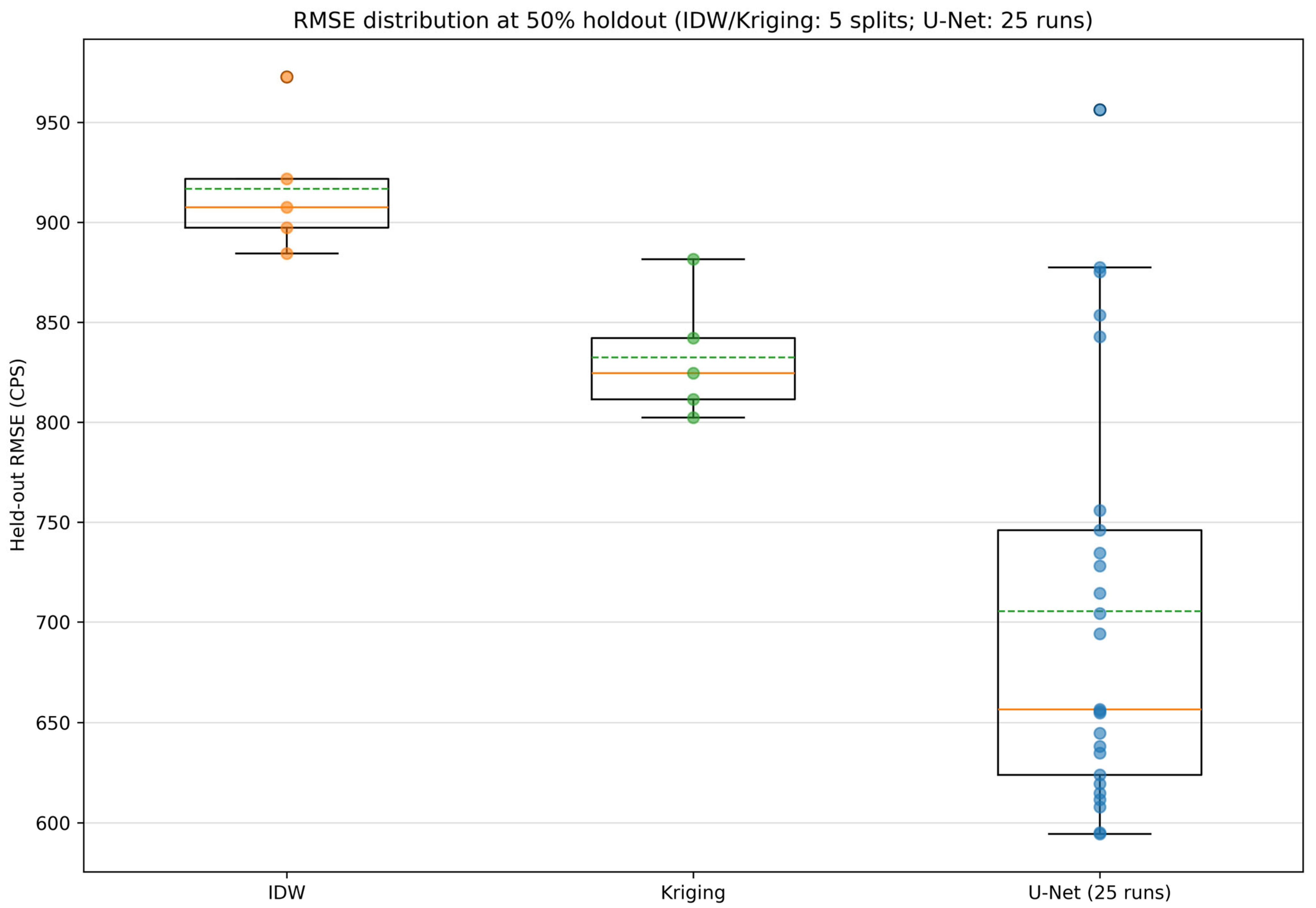
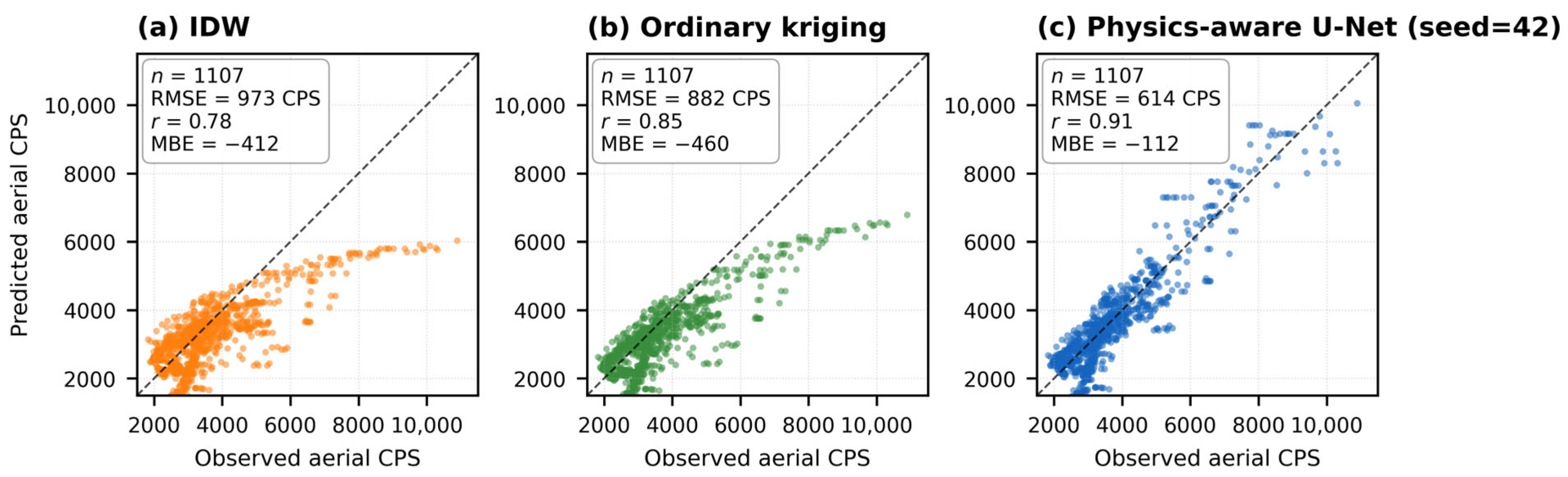
At the 50% held-out benchmark, IDW and ordinary kriging produced mean RMSEs of 916.8 ± 34.2 CPS and 832.4 ± 31.3 CPS, respectively, with mean bias errors of −412 and −460 CPS—persistent underprediction replicated across all five independent data partitions. The scatter plots in Figure 5 reveal structurally similar prediction ceilings—IDW saturating near 5800 CPS and kriging near 6500 CPS—while true values extend to 11,184 CPS. High-CPS observations are not merely scattered around the true values but are systematically compressed. The narrow split-to-split RMSE ranges (IDW 877–952 CPS, Kriging 794–875 CPS, both approximately 4% variation) confirm that these ceilings reflect the methods’ structural properties rather than the particulars of any single data partition. This pattern suggests that the source of error is not the quantity or arrangement of available data but something more fundamental about how conventional interpolators relate aerial observations to the quantity they are intended to estimate.

The underlying cause is the double-blurring mechanism established in Section 1.1 and Section 1.3: each aerial observation A(x, y) = (C * K)(x, y) is already a forward-convolved composite of ground-source contributions, and any conventional interpolator operating in the aerial domain imposes a second spatial averaging on top of it. This compound operation is irreducible: in the limit of complete aerial coverage, IDW and kriging both converge to A(x, y)—the forward-convolved version of the ground source—not to C(x, y) itself. The negative mean biases (~−400 CPS) and the prediction ceilings near 6000 CPS visible in Figure 5a,b are direct signatures of this floor: peaks that forward convolution has spread over a broad footprint cannot be recovered by any method operating exclusively in the aerial domain. Section 3.5.1 demonstrates this directly: kriging is a more accurate aerial interpolator than IDW under PSF-free evaluation (RMSE ratio 2.24× in favour of kriging) but is essentially equivalent under PSF-applied surface estimation (ratio 1.10×); the structural ceiling is shared by both interpolators, not specific to either weighting scheme.

The physics-aware U-Net addresses this at the correct level by learning the inverse of the forward operator: rather than estimating A(x, y) from sparse aerial samples, it estimates C(x, y) directly, then re-projects through K to generate aerial predictions. The forward-consistent training loss (Section 2.3) enforces that the inferred ground field, when forward-projected, is consistent with the observed aerial signal. Because the model operates in the inferred ground domain, it is not constrained by the irreducible forward-convolution floor that limits IDW and kriging.

4.2. What Transferred: Sim-to-Real Fidelity

The consistency across the full 5 split × 5 model seed experimental design—25 out of 25 runs outperforming IDW, mean improvements of approximately 23% over IDW and 15% over kriging—indicates that meaningful inverse deconvolution capability transferred zero-shot from simulation to the real Ukedo survey without any field-based fine-tuning. Variance decomposition confirms that the data partition was not a dominant source of uncertainty: approximately 92% of the total RMSE variance arose from model initialization, with only 6.5% attributable to the choice of data split, indicating that the sim-to-real transfer outcome is robust to the specific random partition but sensitive to the learned feature representation. Three structural properties of the simulation account for this transfer fidelity.

The first is forward kernel fidelity. The physics kernel K was parameterised at h = 30 m and μ = 0.007 m⁻¹, matching the Kim et al. [9] survey (Section 2.2). Because K was identical in simulation and deployment, the inverse deconvolution learned during pretraining remained geometrically valid at deployment: the model entered the field with a correct internal representation of how ground-level contamination maps to aerial counts, requiring no recalibration.

The second is the water-shielding prior. Synthetic hotspot intensities were suppressed at water pixels via the (1 − water_mask) factor (Section 2.2), teaching the model that elevated ground-source values are spatially constrained to land. The real Ukedo river exhibits the same physics, and Channel 2 of the model input provided the same land–water boundary at deployment as during pretraining, preserving the prior exactly.

The third is the sparsity curriculum. Random sparsity masks applied during pretraining retained 10–90% of grid cells per sample. The 50% deployment ratio falls within this range, so the model was not asked to generalise beyond its pretraining experience.

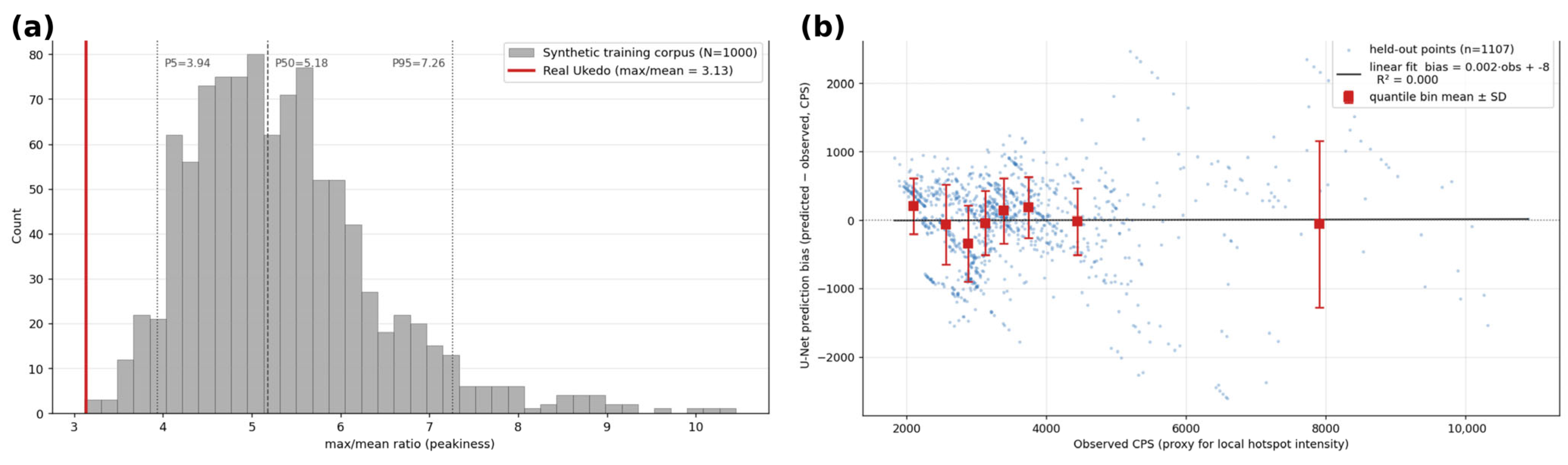
A residual mismatch between the synthetic training distribution and the actual Fukushima contamination pattern is detectable but does not manifest as a calibration bias under ensemble inference. The synthetic ground-source corpus generates max-to-mean ratios in the range [3.94, 7.26] (5th to 95th percentile), while the real Ukedo trajectory has a max-to-mean ratio of 3.13—below the 5th percentile of the synthetic distribution. The primary single-model mean bias of +122 ± 145 CPS (Table 2a) is itself statistically indistinguishable from zero given its variance. Under the ensemble configuration used for the supplementary diagnostics (Section 3.5), the mean bias on held-out points is approximately zero, consistent with the single-model interval. The empirical signature of the distribution mismatch is heteroscedastic prediction variance: the standard deviation of the bias grows by approximately 3× from the lowest-intensity to the highest-intensity quantile (Section 3.5.3, Figure 6). This is the operationally relevant manifestation of the sim–real gap on real-site predictions, and motivates ensemble inference with intensity-dependent uncertainty intervals as the recommended deployment configuration.

4.3. Relationship to the Quantitative Validation Problem in Kim et al. [9]

Kim et al. [9] deployed two independent aerial radiation monitoring systems—the JAEA and KINS platforms—over the Ukedo basin under identical flight conditions, and noted that the resulting maps could not be directly compared at the pixel level because each system projected its measurements onto a distinct grid. The authors identified this as an open methodological problem, observing that there is a need for a method capable of assessing how similar these outcomes are. The Ukedo dataset therefore arrives with an acknowledged absence of a principled quantitative axis for evaluating reconstruction quality. The present study responds to part of this problem: it introduces a within-system held-out validation protocol that provides a quantitative axis for assessing the reconstruction accuracy of a physics-aware model applied to the same survey area. The response is partial by design—the inter-system comparison that Kim et al. [9] were unable to complete is not attempted here.

The within-system held-out correlation reported in Section 3.2 (Pearson r ≈ 0.91 for the physics-aware reconstruction at the same three-model ensemble configuration used for the hotspot diagnostic of Table 2b) and the inter-system correlation reported in Kim et al. [9] measure structurally different quantities. The inter-system metric captures calibration consistency between two physically independent detector systems traversing the same flight path: it is a statement about how reliably the two platforms agree on the same ground-truth signal. The within-system held-out metric captures prediction accuracy of a reconstruction model: given a subset of measurements from one system, how accurately can the model recover the withheld measurements from the same system? These are complementary rather than competing axes. Neither subsumes the other, and a change in one does not imply a corresponding change in the other.

The within-system validation design offers practical advantages in the Ukedo context. It requires only a single survey, bypasses the grid-incompatibility problem that prevented direct map comparison in the original study, and enables quantitative assessment of sparsity robustness across held-out input ratios—a dimension that inter-system comparison cannot provide. Its limitation is symmetrical: it does not measure how a model trained on one system’s survey generalises when evaluated against an independent measurement by a different detector with different calibration characteristics.

The within-system reconstruction axis established here addresses the first of the two gaps identified in Kim et al. [9]; whether the physics-aware model bridges the inter-system calibration gap remains an open question for future work.

4.4. Where the Physics-Aware Reconstruction Adds Value

The supplementary analyses in Section 3.5 localise the practical contribution of the physics-aware reconstruction more precisely than the ~23% mean RMSE improvement reported in Section 3.2. Two findings are particularly informative.

First, the comparison across conventional baselines under both PSF-applied and PSF-free evaluation frames (Section 3.5.1) shows that the structural ceiling that the physics-aware model surpasses is shared by conventional interpolators operating on already forward-convolved aerial observations. Kriging is a more accurate aerial interpolator than IDW under PSF-free evaluation (RMSE ratio 2.24 in favour of kriging) but is essentially equivalent to IDW under PSF-applied surface estimation (ratio 1.10). The mechanism that limits IDW limits kriging in the same way; correcting it requires the inverse deconvolution operation that the U-Net learns from simulation, not a more sophisticated weighting scheme within the same task framing.

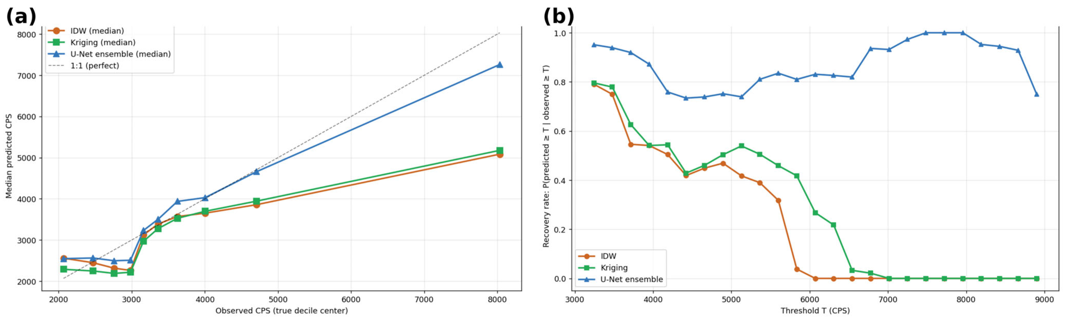
Second, the operationally critical finding is the recovery rate of high-intensity points (Section 3.5.2). At a representative high-intensity threshold near the IDW ceiling (T = 6000 CPS), the IDW recovery rate falls to approximately 0%—the conventional baseline systematically misses points above this threshold—while the U-Net ensemble retains a recovery rate of approximately 80%. The U-Net ensemble ceiling tracks the observed top-decile maximum to within 5.7% headroom, whereas IDW under-shoots by 46.8%. For applications where the operational task is identifying which regions exceed a high-intensity threshold—for example, prioritising sites for further on-ground assessment—this difference is the dominant practical consequence of the method choice. The +23% mean RMSE improvement aggregates across all intensity ranges and consequently understates the gap at the high end of the CPS range.

Together, the two findings reframe the contribution: the physics-aware reconstruction is most valuable not as a uniform improvement over conventional interpolation, but as a recovery of the high-intensity regime that conventional aerial interpolation structurally cannot reach. The ~23% mean improvement is the integrated signature; the recovery rate at high-intensity thresholds is its operational expression.

4.5. What the Ablation and Sensitivity Analyses Reveal

The ablation results (Section 3.6) refine the mechanism claims of Section 4.1 and Section 4.2 in three ways. First, the dominant practical value of the physics-informed input design lies in reliability rather than peak accuracy: removing input priors inflates run-to-run variance far faster than it degrades the mean (±57 → ±530 CPS from full model to plain U-Net), so an unconstrained architecture occasionally matches the full model but cannot be trusted to do so. For operational mapping, where a single deployment-time model must be dependable, this floor-raising property is the operative benefit. Second, the ablation locates the mechanism of physics-awareness more precisely: the forward kernel exerts most of its accuracy influence through data generation—the synthetic supervision pairs already embed the inverse mapping—while the explicit forward-consistency loss contributes calibration (halving the magnitude of the mean bias) and enforces physical self-consistency. This does not diminish the physics-aware framing; the synthetic corpus is itself a product of the forward physics. It does, however, attribute the benefit to the correct component, which matters for future designs that may need to trade the cost of the forward-projection loss term against its calibration value. The non-negativity ablation (A5, Section 3.6) reinforces this localisation: neither output-side constraint—the forward-consistency term or the non-negative activation—carries measurable accuracy benefit on this dataset (the latter never binds, with zero negative predictions in every run), whereas both input-side priors do; output-side physics thus functions as a calibration and plausibility guarantee rather than as an accuracy driver. Third, the plain U-Net variant demonstrates that a modern learning architecture without domain physics is not a dependable alternative on this task (directional advantage 11/25, worst runs exceeding twice the IDW error), complementing the conventional-interpolation comparison of Section 3.1 and Section 3.2 with a learning-based one. Conversely, upgrading the architecture while holding the physics inputs constant (Attention U-Net, Section 3.6) yields no gain beyond run-to-run variance—together, the two comparisons bracket the conclusion that the physics-informed inputs, not the network family, are the operative ingredient. The corpus-sensitivity experiment (Section 3.8) adds that these conclusions are not an artefact of a fortunate synthetic distribution choice: transfer succeeded from all three corpora spanning peakiness medians 3.05–7.67, with only a mild trend favouring peakier corpora.

4.6. Limitations

Several limitations bound the scope of the present study and should be considered when interpreting the results.

Dense surface ground truth is unavailable for the Ukedo basin. No spatially dense surface measurement campaign was conducted at the time of the 2015 aerial survey, which precluded direct pixel-level comparison between the model’s inferred ground field and co-located surface readings. Aerial-domain validation was therefore the only feasible evaluation protocol (Section 2.4). This constraint is partially mitigated by the forward-kernel-consistent evaluation design: withheld aerial measurements were compared against aerial predictions generated by projecting the inferred ground field through the same physics kernel used in training, which ensured that the evaluation criterion was physically commensurate with the measurement process.

Only the KINS system data were used. The JAEA system conducted an independent survey of the same area, but its data were not incorporated. Whether the reconstruction model bridges the inter-system calibration gap was not examined; this is identified as a direction for future work in Section 4.3. More broadly, all results in this study are validated on data acquired by a single monitoring device—the KINS LaBr3(Ce) detector pair described in Section 2.1. The model’s generalisability across different detector systems, with different crystal types, energy responses, and calibration characteristics, remains unconfirmed.

Only total count rate (CPS) was used; the full gamma-ray spectrum was not exploited. Spectral information could in principle distinguish radionuclide contributions and enable energy-specific attenuation corrections, but the present study treats spatial reconstruction independently of spectral decomposition. Spectral-aware reconstruction is a distinct direction outside the scope of this work.

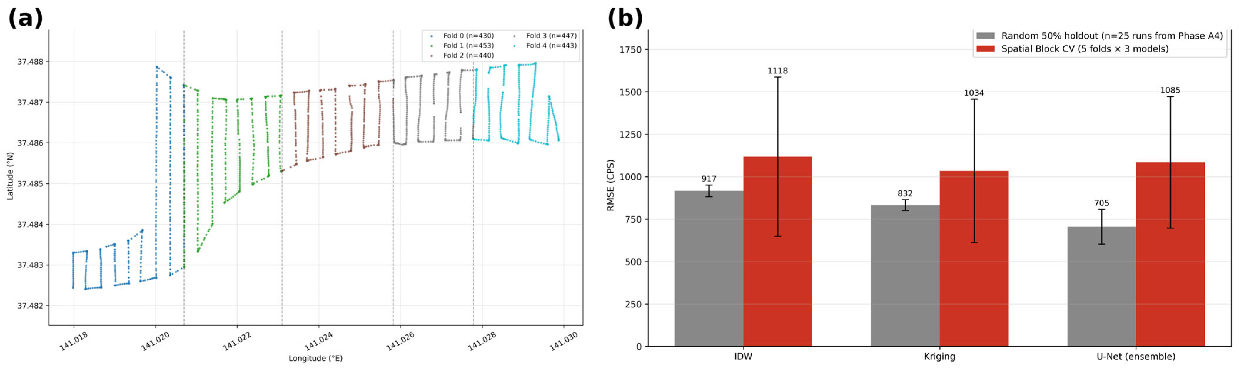
Held-out test points were drawn by random trajectory split, with a spatial blocked stress test now reported inSection 3.5.4. Because the flight trajectory is spatially structured, randomly withheld points may be spatially proximate to training points, which could yield optimistic performance estimates relative to a spatial block cross-validation protocol. We attempted such a protocol (Section 3.5.4) but found that the geometric extent of the PSF kernel is large relative to the achievable exclusion buffer on this dataset, so the blocked test functions as a large-gap extrapolation stress test rather than a definitive spatially independent validation [21,22]. The reported random-holdout correlations and RMSE improvements should therefore be interpreted as upper bounds on what would be obtained under a more stringent spatial holdout protocol of the kind discussed by Wadoux et al. [24], whose suitability depends on the operational task being assessed. A spatially independent evaluation with a redesigned training distribution and a buffer matched to the PSF effective support is identified as a direction for future work in Section 5.

The land–water context encoding is a simplified environmental representation. The two land–water input channels (the scalar prior and the binary water mask) capture only the binary distinction between land and river-channel pixels. Detailed terrain elevation data, vegetation cover, and soil type—all of which influence Cs-137 deposition and retention—were not incorporated. Richer environmental priors could improve reconstruction accuracy, particularly in areas where terrain structure creates systematic deposition gradients.

Performance varies across random seeds. Across the 25 split × model combinations, individual-run RMSE ranged from 577 to approximately 1000 CPS, with within-split standard deviations of approximately 50–150 CPS. The 5 split × 5 model seed design provides evidence of consistent directional improvement (25/25 runs outperforming IDW) but leaves meaningful per-run variance unresolved. Ensemble averaging—adopted for the supplementary analyses (Section 3.5)—substantially reduces this per-evaluation variance, and we recommend ensemble inference for operational use. A larger seed set could further constrain the residual uncertainty.

These limitations define the scope of the present study and suggest concrete directions for future work, including spectral-aware reconstruction, spatial validation protocols, and inter-system generalisation tests.

5. Conclusions

A physics-aware U-Net pretrained entirely on simulation transferred zero-shot to real UAV radiation trajectory data over the Fukushima Ukedo basin, achieving a mean RMSE of approximately 705 CPS at a 50% held-out benchmark across 5 independent data splits with 5 model initializations per split, against approximately 917 CPS for inverse distance weighting and 832 CPS for ordinary kriging—improvements of roughly 23% over IDW and 15% over kriging. Within-system held-out correlation rose from 0.78 (IDW) and 0.85 (Kriging) to 0.91 (U-Net), and the concordance correlation coefficient rose from 0.69 (IDW) and 0.76 (Kriging) to 0.85 (U-Net). The systematic mean bias of the conventional baselines (IDW −412 CPS, Kriging −460 CPS) was reduced to approximately zero under ensemble inference. Directional improvement over IDW was observed in all 25 split × model combinations. Variance decomposition confirmed that approximately 92% of RMSE variance arises from model initialization rather than data partition choice, validating multi-seed replication and motivating ensemble inference as the recommended operational configuration. These conclusions apply to dense flight trajectories and within-coverage reconstruction: as the blocked stress test shows (Section 3.5.4), the advantage over conventional interpolation is drastically reduced under large-gap extrapolation over areas without UAV observations.

The mean negative biases of the two conventional baselines, the structurally similar prediction ceilings of IDW (~5800 CPS) and kriging (~6500 CPS) against measured values reaching 11,184 CPS, and the compression of the kriging-over-IDW advantage from 2.24× under PSF-free evaluation to 1.10× under PSF-applied evaluation (Section 3.5.1) together confirm that the limitation of conventional interpolation for surface reconstruction from forward-convolved aerial measurements is structural and shared across IDW and kriging. Interpolating already-convolved aerial measurements imposes a second spatial averaging that cannot resolve the underlying ground source regardless of measurement density or weighting scheme. Physics-aware inverse deconvolution addresses this at the correct level by learning to invert the forward operator directly. The operational expression of this difference is the recovery of high-intensity hotspots: at a representative threshold near the IDW ceiling (T = 6000 CPS) the IDW recovery rate falls to approximately 0% while the U-Net ensemble retains approximately 80% (Section 3.5.2), which is the practical consequence most relevant to applications that prioritise reliable identification of high-intensity regions in post-accident contamination mapping.

Several directions follow naturally from this work. Inter-system validation using the independent JAEA survey would test whether the reconstruction is consistent with a physically distinct detector calibration (Section 4.3). Spatially independent evaluation with a buffer matched to the PSF effective support would provide a more stringent generalisation bound than the random-holdout protocol used here; given the kernel’s geometric extent on this dataset, this likely requires either a thinned-observation block design [22] or coarser folds with a redesigned training distribution that includes contiguous-block sparsity patterns—the first-pass blocked stress test reported in Section 3.5.4 illustrates the protocol challenges. Spectral-aware reconstruction, exploiting the full gamma-ray spectrum rather than total count rate, could improve accuracy in radiologically complex environments. Ensemble averaging across larger model populations would further reduce the per-seed performance variance reported here. Application to broader site geometries—including forested terrain with simultaneous LiDAR-derived elevation and vegetation models—is enabled by the physics-aware framework’s modular treatment of environmental priors.