Supraglacial Lake Bathymetry Retrieval from ICESat-2 Altimetry Data and Sentinel-2 Imagery Using Deep Learning Algorithms

Highlights

What are the main findings?

• An integrated framework was developed for supraglacial lake mapping and bathymetry retrieval using ICESat-2 altimetry and Sentinel-2 imagery.
• The residual dense network achieved the best average performance across the four investigated lakes, with mean R², RMSE, and MAE of 0.927, 0.187 m, and 0.144 m.

What are the implications of the main findings?

• For the four investigated lakes, the proposed multi-source framework extends sparse along-track photon-derived depths into spatially continuous supraglacial lake bathymetry maps.
• The framework demonstrates the potential to provide bathymetric inputs for future lake-water-storage estimation and ice-shelf hydrological analysis in data-limited Antarctic environments.

Abstract

Supraglacial lake depth is a key variable for quantifying surface meltwater storage and assessing ice-shelf stability, yet spatially continuous and reliable bathymetric information remains difficult to obtain in polar regions because in situ measurements are scarce and optical imagery cannot directly provide water depth. This study develops an integrated framework for supraglacial lake identification and bathymetry retrieval by combining ICESat-2 ATL03 photon-counting lidar data with Sentinel-2 multispectral imagery. ICESat-2 lake photons were used to constrain lake-region extraction from Sentinel-2 imagery, and the photon-derived along-track depths were corrected for scattering and refraction before being converted into Sentinel-2 pixel-level depth labels. Based on these labels, four retrieval models were constructed and evaluated, including an empirical model, CatBoost, a convolutional neural network (CNN), and a residual dense network (RDN). CatBoost generated initial depth estimates, while CNN and RDN further incorporated the CatBoost-derived depth prior and Sentinel-2 multispectral features for pixel-level depth prediction. Experiments over four investigated supraglacial lakes showed that RDN achieved the best average performance across the investigated lakes, with mean R², RMSE, and MAE values of 0.927, 0.187 m, and 0.144 m, respectively. For the investigated lakes, the integration of ICESat-2 and Sentinel-2 extended discrete along-track reference-depth observations to spatially continuous bathymetry maps. Because the training and validation samples were obtained from different spatial blocks within the same four lake scenes, the reported performance primarily reflects within-lake spatial generalization under the investigated conditions, and transferability to unseen lakes remains to be evaluated. These maps may provide inputs for future lake-volume estimation and ice-shelf hydrological analyses, while their applicability to lakes with different morphological and optical conditions requires further evaluation.

1. Introduction

The Lambert–Amery system, which contains the Amery Ice Shelf, drains approximately 16% of the East Antarctic Ice Sheet and represents one of the most important ice-sheet–ice-shelf drainage systems in East Antarctica [1]. Variations in surface meltwater and supraglacial lakes over this region are therefore closely related to ice-shelf stability and surface water storage assessment. In a warming climate, the Greenland and Antarctic ice sheets are undergoing rapid mass loss, accompanied by increasingly widespread surface melting [2,3,4]. Supraglacial lakes are widely distributed on both ice sheets. By lowering surface albedo, supraglacial lakes increase the absorption of shortwave radiation, creating a positive feedback loop that further enhances surface melting. On ice shelves, the accumulation and drainage of supraglacial lake water may also promote hydrofracturing and affect ice-shelf stability [5,6]. Accurate estimates of supraglacial lake depth and water volume are therefore essential for quantifying surface meltwater storage and constraining coupled hydrological–dynamical models [7,8]. However, direct lake-depth observations remain extremely limited in polar regions. In situ measurements over Antarctic ice shelves are still largely unavailable, while only a small number of supraglacial lakes in Greenland have been surveyed. This lack of direct depth observations remains a major source of uncertainty in estimating ice-sheet surface water storage, highlighting the need for reliable supraglacial lake bathymetry mapping, particularly over Antarctic ice shelves.

A range of methods has been developed to estimate supraglacial lake depth and volume, including field measurements, optical remote sensing, and satellite altimetry. Field-based approaches, such as sonar and radiometric measurements, can provide highly accurate depth observations [9,10], but their applications are limited by high cost, logistical constraints, and harsh polar environments. Optical remote sensing has been widely used because it provides repeated observations over large areas [11,12,13,14]. Existing optical approaches mainly include physically based models derived from the Bouguer–Lambert–Beer law and empirical models that relate spectral reflectance to measured water depth [15,16]. However, optical depth retrieval is strongly affected by water optical properties, lake-bottom reflectance, thin ice cover, and mixed pixels. Its sensitivity also decreases for deeper water, often leading to depth underestimation when lake depth exceeds approximately 5 m, with errors potentially exceeding 1 m [17]. In the absence of sufficient in situ measurements, the accuracy of optical depth retrieval alone is difficult to guarantee, indicating the need to combine optical imagery with independent elevation or depth observations.

ICESat-2, launched in 2018, has provided new opportunities for supraglacial lake bathymetry. Its Advanced Topographic Laser Altimeter System (ATLAS) uses a 532 nm green laser that can penetrate clear water and record photon returns from both the lake surface and the lake bottom, enabling direct estimation of lake depth along the satellite ground track [18,19,20]. Under favorable conditions, ICESat-2 has been shown to retrieve water depths of up to 41 m, with typical depth errors of approximately 0.5 m [21].

Several algorithms have been developed to retrieve supraglacial lake depths from ICESat-2 ATL03 photon cloud data. According to their degree of automation, these methods can be broadly divided into automated or low-intervention approaches and semi-automatic approaches that require prior lake-location information. The ATL13 inland water product represents an automated processing approach [22], whereas adapted ATL08 and the lake surface–bed separation algorithm requires additional lake identification or manual intervention [18,23]. Fricker et al. [19] compared several methods with manually extracted depths for Antarctic supraglacial lakes and found that adapted ATL08 achieved high accuracy, although manual lake identification was still required. The Watta algorithm applies kernel density estimation to automatically extract lake-surface and lake-bottom photons [24], but it is sensitive to outliers and may overfit where bottom photons are sparse [19]. The automated lake detection algorithm identifies lake locations using surface flatness and bottom photon counts and achieves RMSE values of approximately 0.30–0.32 m for lakes in Greenland and Antarctica, with a maximum detected depth of 8.25 m [20]. The FLUID–SuRRF framework further supports large-scale supraglacial lake detection and depth retrieval by combining flat-surface detection with robust fitting of lake-surface and lake-bottom elevations [25]. Nevertheless, algorithms that rely strongly on surface flatness or photon density may still suffer from false detections or missed detections, particularly for shallow lakes or lakes with complex spectral conditions.

Despite these advances, large-scale and fully automated processing of ICESat-2 ATL03 data remains challenging. The ATL03 product contains hundreds of terabytes of unstructured photon cloud data, and many existing studies still focus on a limited number of manually selected lakes or track segments [26]. In addition, ICESat-2 provides only sparse along-track observations, with an across-track spacing of approximately 3.3 km and a 91-day repeat cycle. As a result, ICESat-2 alone cannot provide spatially continuous monitoring of supraglacial lake water storage across entire ice shelves or ice sheets. Combining ICESat-2 with optical satellite imagery offers a promising way to overcome these limitations. ICESat-2 provides along-track depth observations, whereas Sentinel-2 provides continuous multispectral coverage over lake surfaces. This combination can compensate for the limited spatial coverage of ICESat-2 and the lack of direct depth information in optical imagery, enabling the extension of discrete laser-derived depth observations to spatially continuous bathymetric maps. Previous studies have used ICESat-2-derived depths as training labels for optical image-based models, allowing along-track depth measurements to be extended to whole-lake or regional scales [24,27,28]. In such approaches, synchronous or near-synchronous optical imagery provides spectral reflectance and derived indices as input features, while ICESat-2 depth estimates serve as reference labels. Machine learning models can then be trained to learn the nonlinear relationship between spectral information and water depth and applied to the full image coverage to generate spatially continuous lake depth distributions.

Machine learning methods have shown potential for supraglacial lake mapping and depth retrieval. Zhao et al. [29] used a random forest model to retrieve the depths of Greenland ice-marginal lakes and reported R² values of 0.82–0.86 and RMSE values of approximately 0.35–0.37 m for four lakes. Although random forest showed good stability and feature interpretability, its ability to represent spatial heterogeneity remained limited compared with geographically weighted random forest. Feng et al. [30] applied random forest to supraglacial lake area extraction using multi-temporal Sentinel-2 imagery in southwestern Greenland and achieved an average intersection over union of 90.20%, demonstrating the reliability of random forest for water-body identification in ice and snow environments. Zhang et al. [31] compared support vector regression with several tree-based models for supraglacial lake depth retrieval on the Amery Ice Shelf and found that CatBoost and XGBoost outperformed the original SVR model. Although Bayesian optimization substantially improved SVR performance, the sensitivity of SVR to hyperparameters and its relatively low computational efficiency may limit its applicability in large-scale retrieval tasks. The better performance of CatBoost and XGBoost further indicates the potential of tree-based models for supraglacial lake depth estimation. These studies indicate that machine learning can effectively model nonlinear relationships between optical features and lake depth, but model performance may vary with lake conditions, sample distribution, and spatial heterogeneity.

Compared with empirical and conventional machine-learning models, deep-learning models can learn multi-level spectral–spatial representations from multispectral image patches. However, their transferability depends on the diversity of the training samples and the consistency of lake morphology, depth range, optical properties, and photon-sampling conditions between the training and target lakes. This study develops an integrated framework for supraglacial lake identification and bathymetry retrieval using ICESat-2 ATL03 photon data and Sentinel-2 multispectral imagery. The framework identifies lake photons along ICESat-2 tracks, extracts lake regions from Sentinel-2 imagery using photon-constrained spectral information, and converts corrected ICESat-2 along-track depths into Sentinel-2 pixel-level depth labels. Based on these labels, an empirical model, CatBoost, CNN, and RDN are constructed and compared for lake depth retrieval. The integration of photon-constrained lake-region extraction, scattering- and refraction-corrected pixel-level depth labels, and CatBoost-guided spectral–spatial refinement provides a unified pathway for extending sparse ICESat-2 depth observations to spatially continuous supraglacial lake bathymetry. The objective of this study is to develop and evaluate an integrated workflow for identifying supraglacial lakes and extending discrete ICESat-2 along-track depth observations to spatially continuous bathymetry maps for four investigated lakes on the Amery Ice Shelf. The resulting bathymetry maps may provide inputs for future lake-volume estimation and ice-shelf hydrological analyses.

2. Materials and Methods

2.1. Study Area and Data

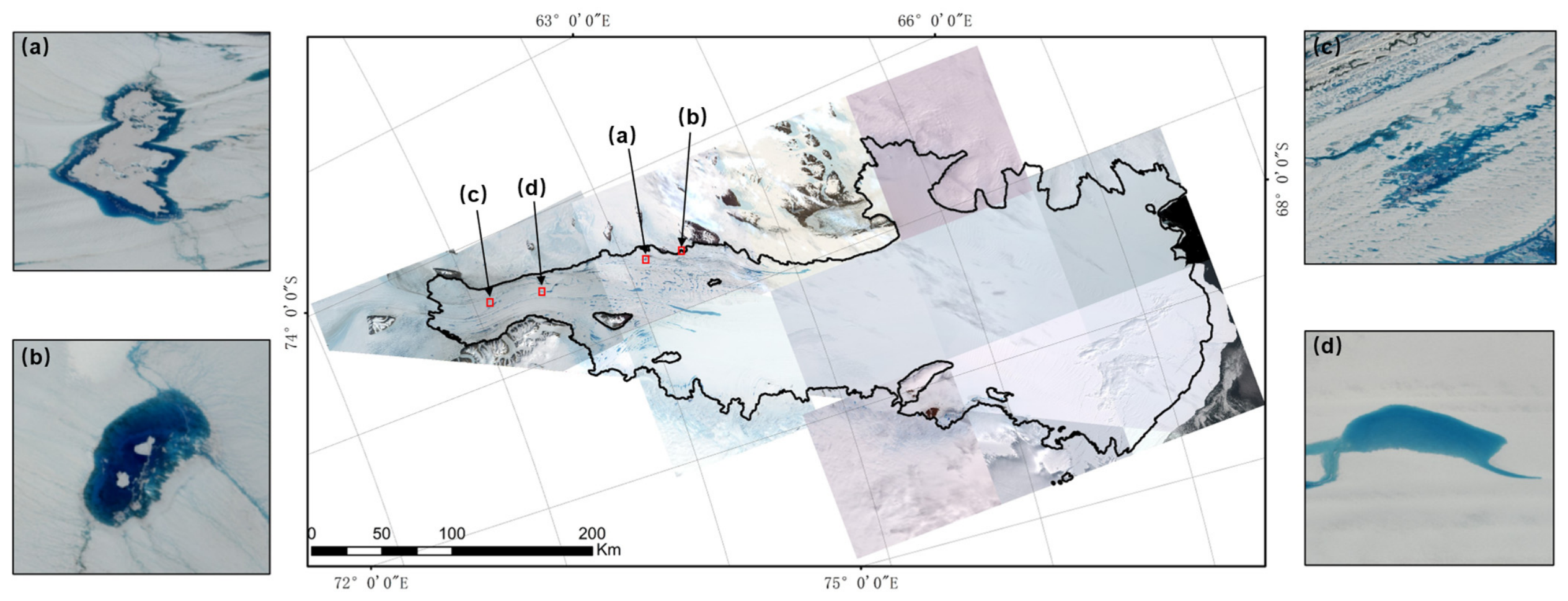
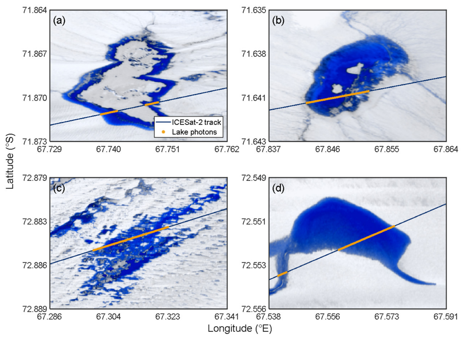
The study area is located on the Amery Ice Shelf in East Antarctica, which forms part of the Lambert–Amery drainage system. During the austral summer, extensive surface melting occurs over the ice shelf and produces numerous supraglacial lakes [1,19]. As shown in Figure 1, four supraglacial lakes intersected by ICESat-2 ground tracks were investigated in this study and are hereafter referred to as Lakes 1–4.

To minimize temporal inconsistencies between the laser-altimetry observations and optical imagery, ICESat-2 ATL03 data and Sentinel-2 Level-1C imagery acquired on 2 January 2019 were used for all four lakes. The Sentinel-2 imagery was acquired under limited cloud interference and adequate solar-illumination conditions. Although local thin-ice cover was present over portions of some lakes, the principal open-water areas and lake boundaries remained identifiable. The investigated lakes were intersected by ICESat-2 ground tracks, exhibited identifiable lake-surface and lake-bottom photon returns, and provided sufficient valid depth samples for matching with the Sentinel-2 pixels. As summarized in

Table 1. Geographic and data information for the four investigated supraglacial lakes.

Lake	Latitude (°S)	Longitude (°E)	Lake Area (km2)	ICESat-2 ATL03	Sentinel-2 Image
Lake 1	71.864–71.873	67.729–67.762	0.8206	20190102184312	20190102T041719
Lake 2	71.635–71.643	67.837–67.864	1.2649	20190102184312	20190102T041719
Lake 3	72.879–72.889	67.286–67.341	3.5025	20190102184312	20190102T041719
Lake 4	72.549–72.556	67.538–67.591	2.5752	20190102184312	20190102T041719

, the four lakes differed in geographic extent and area but were analysed using contemporaneous ICESat-2 and Sentinel-2 observations.

2.2. Framework Overview

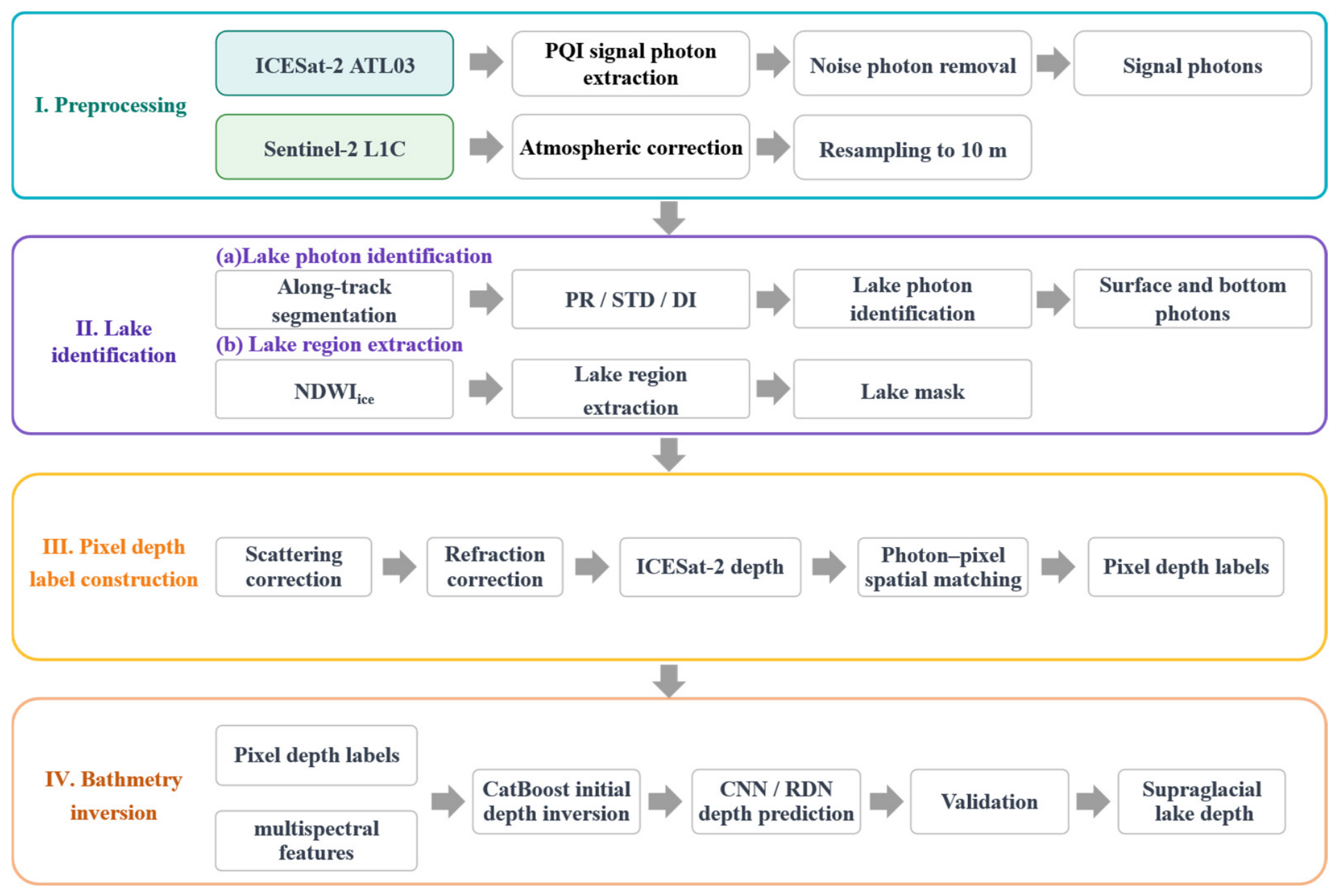
This study develops an integrated framework for automated supraglacial lake identification and bathymetry retrieval and evaluates it over four investigated lakes on the Amery Ice Shelf using ICESat-2 ATL03 photon data and Sentinel-2 multispectral imagery. ICESat-2 provides accurate along-track depth observations, whereas Sentinel-2 offers spatially continuous multispectral information over lake surfaces. By combining these two datasets, the proposed framework compensates for the sparse spatial coverage of ICESat-2 and the lack of direct depth information in optical imagery, enabling discrete photon-derived depth observations to be extended to spatially continuous lake bathymetry maps. As shown in Figure 2, the workflow consists of four main components: data preprocessing, lake photon identification and lake-region extraction, pixel-level depth label construction, and bathymetry inversion.

2.3. Preprocessing

Sentinel-2 multispectral imagery and ICESat-2 ATL03 photon data were preprocessed to provide consistent inputs for lake identification and bathymetry retrieval. For Sentinel-2 imagery, Level-1C products were atmospherically corrected using Sen2Cor v2.12.04 to generate Level-2A surface reflectance products. The selected bands were reprojected to the Antarctic Polar Stereographic coordinate system (EPSG:3031) and resampled to a common spatial resolution of 10 m using bilinear interpolation [31,32]. Before subsequent analysis, the scaled Level-2A reflectance values were divided by 10,000, and pixels with invalid or missing observations were excluded. In this study, four 10 m spectral bands, namely B2, B3, B4, and B8, were retained for subsequent processing. B2 and B4 were used to calculate $NDW{I}_{\mathrm{i}\mathrm{c}\mathrm{e}}$ for lake-region extraction, whereas the selected bands were used as multispectral inputs for bathymetry retrieval. The 10 m spatial resolution was retained because all four selected bands are natively available at this resolution, providing a consistent pixel grid for matching the ICESat-2-derived depth observations with Sentinel-2 imagery.

For ICESat-2 ATL03 data, photon longitude, latitude, elevation, along-track distance, photon ID, and related geometric information were extracted within the target study area. The raw photons were spatially clipped according to the study-area extent and candidate lake regions to reduce the influence of irrelevant photons outside the regions of interest. Because the original ATL03 photon cloud contains atmospheric scattering photons, background noise, and anomalous-elevation photons, it cannot be directly used for lake detection or depth estimation.

The pre-pruning quadtree isolation (PQI) method was therefore applied to extract signal photons [33]. This method separates signal photons from noise photons according to their spatial isolation characteristics, allowing ice-surface, lake-surface, and subsurface returns to be retained without relying on a fixed density threshold. The extracted signal photons were used as the input for subsequent lake photon identification.

2.4. Lake Identification

After signal photon extraction, lake photons were identified along the ICESat-2 ground track. The signal photons were divided into 10 m along-track segments, and the photon density and elevation standard deviation were calculated for each segment. In supraglacial lake areas, lake-surface and subsurface photon returns are often present simultaneously, producing a more dispersed elevation distribution than that over the surrounding snow and ice surfaces. The local photon density may also vary markedly in these areas. Based on these characteristics, the PR, STD, and DI metrics were used to identify lake segments [31,34]. The DI metric is defined as follows:

$$DI={\displaystyle \frac{{PR}_i-{PR}_{min}}{{PR}_{max}-{PR}_{min}}}\cdot {\displaystyle \frac{{STD}_i-{STD}_{min}}{{STD}_{max}-{STD}_{min}}}$$

(1)

where $P{R}_i$ and $ST{D}_i$ denote the photon density and elevation standard deviation of the $i$-th segment, respectively. $P{R}_{\mathrm{m}\mathrm{a}\mathrm{x}}$, $P{R}_{\mathrm{m}\mathrm{i}\mathrm{n}}$, $ST{D}_{\mathrm{m}\mathrm{a}\mathrm{x}}$, and $ST{D}_{\mathrm{m}\mathrm{i}\mathrm{n}}$ represent the maximum and minimum values of the corresponding metrics among all segments. To reduce short-scale fluctuations, the segment-level PR and STD sequences and the resulting DI series were smoothed using moving windows. An adaptive DI threshold was then determined using Otsu’s method, and segments exceeding this threshold were identified as candidate lake segments. Short gaps between candidate segments were connected, whereas isolated short segments were removed to improve the along-track continuity of the identified lake regions.

The along-track lake photon results were then integrated with Sentinel-2 imagery to extend ICESat-2-based lake detection from discrete ground-track observations to two-dimensional lake-region mapping. Supraglacial lakes on ice shelves exhibit spectral characteristics that differ from those of the surrounding snow and ice surfaces, making Sentinel-2 imagery suitable for lake extraction. However, lake boundaries are often affected by thin ice cover, wet snow, shadows, and mixed pixels, which makes it difficult to apply a single fixed spectral threshold consistently across different lakes. To improve the robustness of lake-region extraction, the ICESat-2 lake photon results were used as observational constraints in the Sentinel-2 image segmentation process.

The ice-surface normalized difference water index, $NDW{I}_{ice}$, was used to enhance the spectral contrast between lake water and the surrounding snow and ice background [35]:

$${NDWI}_{ice}={\displaystyle \frac{B_2-B_4}{B_2+B_4}}$$

(2)

where $B_2$ and $B_4$ denote the Sentinel-2 blue and red band reflectance, respectively. The identified ICESat-2 lake photons were projected onto the Sentinel-2 image grid to identify the candidate lake regions intersected by the satellite ground track. Within each candidate region, an adaptive threshold was determined from the local $NDW{I}_{\mathrm{i}\mathrm{c}\mathrm{e}}$ distribution using Otsu’s method, with the projected photon locations providing along-track constraints for the corresponding lake region [31]. Compared with fixed-threshold segmentation, this strategy reduces the sensitivity of threshold selection to spectral variability among different lakes.

Pixel classification was performed only within candidate lake regions to minimize interference from adjacent ice surfaces, wet snow, and non-lake areas. After the initial lake mask was generated, small isolated patches were removed and morphological smoothing was applied to improve the spatial continuity of the extracted lake regions. The final lake mask was used to constrain subsequent photon filtering, depth sample generation, and bathymetry retrieval.

2.5. Pixel Depth Label Construction

After lake photon identification and lake-region extraction, photons within the lake mask were further classified into lake-surface photons, candidate lake-bottom photons, and scattering photons. Lake-surface photons were identified from the elevation distribution of lake photons. Because surface returns are usually concentrated around the dominant peak of the elevation histogram, a Gaussian distribution was fitted to this peak to determine the lake-surface elevation range. Photons within this range were classified as lake-surface photons, whereas photons below this range were treated as candidate lake-bottom photons or scattering photons [36].

When the ICESat-2 laser pulse enters the water column, it can be affected by water-column scattering and scattering from lake-bottom ice. As a result, candidate bottom photons may include scattering photons located below the actual lake bottom [37,38]. Directly fitting the lake bottom using these photons may bias the estimated bottom elevation downward and consequently overestimate water depth. To reduce this effect, a cloth-simulation-based scattering correction method was used to extract lake-bottom photons with reduced influence from sub-bottom scattering [39,40]. A continuous lake-bottom support profile was first constructed from the candidate bottom photons using the cloth-simulation method. Photons consistent with the fitted profile and the local along-track continuity were retained as valid lake-bottom photons, whereas isolated deeper returns were removed as scattering photons.

The scattering-corrected lake-bottom photons were subsequently corrected using Snell’s law, with the ATL03 reference elevation angle and refractive indices of 1.000 and 1.334 for air and water, respectively [41]. The corrected water depth was calculated as the vertical elevation difference between the lake surface and the refraction-corrected lake bottom. After scattering and refraction corrections, the photon elevation profiles were converted into along-track reference-depth observations for pixel-level label construction.

To use ICESat-2-derived depths for Sentinel-2-based bathymetry retrieval, pixel-level depth labels were constructed. The corrected depth samples were projected onto the Sentinel-2 image coordinate system and assigned to 10 m image pixels. When multiple valid depth samples fell within the same pixel, their mean value was used as the final depth label of that pixel. To quantify the random uncertainty associated with photon sampling and pixel-level aggregation, a nonparametric bootstrap analysis was conducted for each pixel containing at least two corrected photon-depth observations. The observations within each pixel were resampled with replacement 2000 times using a fixed random seed of 42, and the mean water depth was recalculated for each resample. The standard deviation of the bootstrap means was taken as the pixel-level sampling uncertainty, and the 2.5th and 97.5th percentiles were used to define the 95% confidence interval. Pixels containing a single corrected photon-depth observation were retained as depth labels but excluded from the bootstrap uncertainty calculation. This procedure converted discrete ICESat-2 along-track depth observations into Sentinel-2 pixel-level depth labels and linked them with the corresponding multispectral reflectance features, providing supervised samples for subsequent machine learning and deep learning models.

2.6. Bathymetry Inversion

After the Sentinel-2 pixel-level depth labels were generated, four bathymetry retrieval models were constructed, including an empirical model, CatBoost, a convolutional neural network (CNN), and a residual dense network (RDN). The empirical model was used as a conventional optical bathymetry baseline to describe the logarithmic relationship between multispectral reflectance and water depth. CatBoost was used to model the nonlinear relationship between Sentinel-2 reflectance and pixel-level depth labels and to generate an initial depth estimate. CNN and RDN further used Sentinel-2 multispectral imagery together with the CatBoost-derived initial depth as inputs to predict pixel-level lake depth. Therefore, CNN and RDN constitute second-stage retrieval models that depend on the CatBoost-derived initial depth rather than fully independent bathymetry-retrieval pipelines. The main idea was to first obtain a stable initial depth prior using a machine learning model and then incorporate local spatial information through deep learning models to reduce local biases in the initial retrieval results.

2.6.1. Empirical Model

The empirical model was constructed following the classical multispectral bathymetry approach proposed by Lyzenga [42], in which logarithmically transformed spectral reflectance is related to water depth through a linear regression model. Sentinel-2 bands B2, B3, and B8 were selected to construct the three-band logarithmic linear model. The blue and green bands provide the primary depth-related information because of their relatively greater penetration in water. Although near-infrared radiation is strongly attenuated by water, B8 was retained as a complementary spectral variable because of its strong contrast between open water and the surrounding snow and ice surfaces. This contrast can help account for spectral variability associated with shallow water, lake margins, and mixed ice–water pixels [30]. The model is formulated as follows:

$$d=b_0+b_1\ln \left(B_2\right)+b_2\ln \left(B_3\right)+b_3\ln \left(B_8\right)$$

(3)

where d is the retrieved water depth; $B_2$, $B_3$, and $B_8$ denote the surface reflectance of the Sentinel-2 blue, green, and near-infrared bands, respectively; $b_0$ is the intercept; and $b_1$, $b_2$, and $b_3$ are regression coefficients. The model coefficients were determined using least-squares regression based on the ICESat-2 pixel-level depth labels and the corresponding spectral reflectance values. Owing to its simple structure, this empirical model was used as a conventional optical bathymetry baseline.

2.6.2. CatBoost-Based Initial Depth Inversion

The relationship between supraglacial lake depth and multispectral reflectance is nonlinear and can be affected by water-column scattering, lake-bottom reflectance, thin ice cover, and mixed pixels. Therefore, CatBoost was used to construct the initial depth inversion model. CatBoost is a gradient-boosted decision tree algorithm that can improve nonlinear fitting capability by iteratively combining multiple regression trees and can remain stable under limited training samples [43]. For the $i$-th training pixel, the input feature vector is expressed as:

$$X_i={\left[B_2,B_3,B_4,B_8\right]}_i$$

(4)

where $B_2$, $B_3$, $B_4$, and $B_8$ denote the surface reflectance of the selected Sentinel-2 bands. The ICESat-2 pixel-level depth label $d_i$ was used as the supervised target to train the CatBoost model. The predicted depth can be written as:

$${\widehat{d}}_i^0=F_{cat}\left(X_i\right)$$

(5)

where ${\widehat{d}}_i^0$ is the initial depth estimated by CatBoost, and $F_{cat}(\cdot )$ denotes the trained CatBoost regression model. The CatBoost-derived depth result was used both as an independent machine-learning result for comparison and as the initial depth prior for the subsequent CNN and RDN models. The spatially blocked 80:20 split was performed before model fitting. For each lake, a separate CatBoost model was trained exclusively on the training subset and then applied to all valid lake pixels to generate the initial-depth prior map. Accordingly, the prior values at validation locations were generated without using the corresponding validation depth labels. The same held-out validation subset was used to evaluate all four models. The CatBoost model was trained using 500 boosting iterations, a learning rate of 0.03, a maximum tree depth of 6, and the RMSE loss function. The random seed was fixed at 42, and no automated hyperparameter optimization was applied.

2.6.3. CNN Depth Prediction

To incorporate local spatial information from Sentinel-2 imagery, a convolutional neural network was used as the deep learning baseline [44]. The input feature tensor of the CNN was constructed by stacking the Sentinel-2 multispectral image patch and the CatBoost-derived initial depth map along the channel dimension:

$$X=\mathrm{Concat}\left(S,D_0\right)$$

(6)

where $S$ denotes the Sentinel-2 multispectral image patch, $D_0$ is the initial depth map predicted by CatBoost, and $\mathrm{C}\mathrm{o}\mathrm{n}\mathrm{c}\mathrm{a}\mathrm{t}(\cdot )$ represents channel-wise concatenation. The CatBoost-derived depth map was reprojected onto the corresponding Sentinel-2 image-patch grid using bilinear resampling. Before channel-wise concatenation, the depth values were divided by 10 and clipped to the range of 0–1. CNN extracts local spectral–spatial features through convolutional layers and nonlinear activation functions and outputs a single-channel pixel-level depth map. Compared with CatBoost, which mainly relies on single-pixel spectral features, CNN can use neighborhood information and therefore serves as a baseline for evaluating the effect of basic convolutional spatial feature extraction.

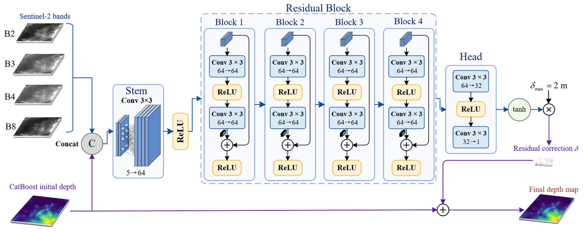
The CNN received a 32 × 32-pixel five-channel input tensor consisting of Sentinel-2 bands B2, B3, B4, and B8 and one normalized CatBoost-derived initial-depth channel. The network used 64 base feature channels and four residual blocks. Each residual block contained two 3 × 3 convolutional layers with ReLU activation and an identity shortcut connection. The network comprised one input convolutional layer, eight convolutional layers within the four residual blocks, and two output-head convolutional layers, giving 11 convolutional layers in total. The output head predicted a spatially varying residual correction, which was constrained to ±2 m using a hyperbolic tangent function. The correction was added to the CatBoost-derived initial depth. This configuration resulted in a total of 317,121 trainable parameters.

2.6.4. RDN Depth Prediction

To further enhance spatial feature representation, a residual dense network was introduced to improve feature propagation and feature reuse across different network layers [45]. The RDN used the same input configuration as the CNN, consisting of the four-band Sentinel-2 image patch and the CatBoost-derived initial depth map. Compared with a conventional CNN, the main architectural distinction of RDN lies in its residual dense blocks, which can integrate shallow spectral information with deeper spatial representations. This structure is expected to improve the model’s ability to represent local depth variations in supraglacial lakes.

The RDN architecture consisted of four main components: shallow feature extraction, residual dense feature extraction, global feature fusion, and depth reconstruction. First, the input tensor was passed through convolutional layers to extract shallow features. These features were then fed into a series of residual dense blocks, where dense connections were used to reuse multi-level features and local residual learning was applied to preserve the input information of each block. The outputs of different residual dense blocks were subsequently integrated through a global feature fusion module, followed by an output convolution layer to generate the final depth prediction map. This process can be expressed as:

$${\widehat{\mathrm{D}}}_{RDN}=H_{out}\left(H_{GFF}\left(H_{RDB}\right(X\left)\right)+F_s\right)$$

(7)

where ${\widehat{D}}_{RDN}$ denotes the depth map predicted by the RDN, $X$ is the network input, $H_{RDB}(\cdot )$ represents residual dense feature extraction, $H_{GFF}(\cdot )$ denotes global feature fusion, $F_s$ is the shallow feature, and $H_{out}(\cdot )$ represents the depth reconstruction mapping. Through local dense connections and global feature fusion, RDN can combine shallow spectral information, deep spatial features, and the CatBoost-derived initial depth prior, thereby improving the stability of depth retrieval under complex lake conditions.

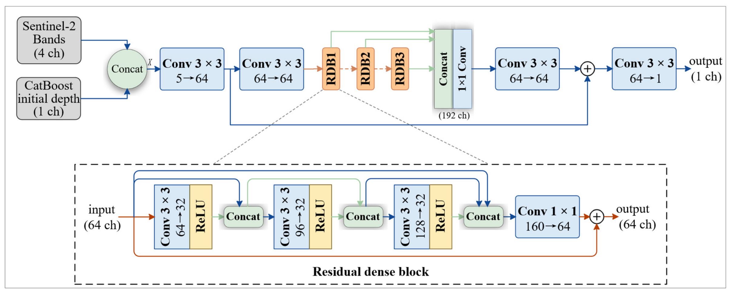
The RDN used the same five-channel input configuration as the CNN. Unlike the CNN, which predicts a bounded residual correction that is added to the CatBoost-derived initial depth, the RDN directly reconstructs the final depth map by integrating the normalized initial-depth prior with multi-level spectral–spatial features. It contained two shallow-feature 3 × 3 convolutional layers followed by three residual dense blocks. Each residual dense block comprised three densely connected 3 × 3 convolutional layers with ReLU activation, 64 base feature channels, a growth rate of 32, a 1 × 1 local feature-fusion convolution, and a local residual connection. The outputs of the three residual dense blocks were concatenated and integrated using 1 × 1 and 3 × 3 global feature-fusion convolutions, followed by a final 3 × 3 convolution for depth reconstruction. Including the 1 × 1 local and global feature-fusion layers, the RDN contained 17 convolutional layers in total. The complete RDN contained 369,281 trainable parameters.

2.6.5. Deep-Learning Model Training

Before image-patch generation, the pixel-level depth samples were partitioned into training and validation subsets using the spatial-block strategy. Only the training subset was used to construct the training image patches and sparse depth-label maps. The CNN and RDN models were trained separately for each lake using the corresponding lake-specific training samples. Both CNN and RDN used image patches of 32 × 32 Sentinel-2 pixels, corresponding to approximately 320 m × 320 m at the 10 m spatial resolution. No fixed sliding-window stride was used; instead, each valid training-label pixel was treated as the center of a candidate patch. Patches with identical upper-left coordinates were retained only once, whereas patches extending beyond the image boundaries were discarded. Because the patches were centered on valid training-label pixels, the multispectral context contained in neighboring patches could partially overlap. Training patches were not generated around unlabeled center pixels, although unlabeled pixels could occur within the surrounding image context and were excluded from the supervised loss through the validity mask.

A candidate patch was retained only when it contained at least one valid depth label, lake-region pixels covering at least 5% of the patch area, and valid multispectral observations in at least 30% of its pixels. Patches intersecting the lake boundaries were retained only when they satisfied the same lake-region coverage criterion. Sparse supervision masks were generated exclusively from the depth labels assigned to the training subset, whereas the validation labels were reserved for model evaluation and were not included in the training loss. Because the training and validation samples were obtained from different spatial blocks within the same lake scenes, the resulting assessment represents within-lake spatial validation rather than scene-independent testing.

Data augmentation was applied only to the four Sentinel-2 reflectance channels during training. The augmentation included random multiplicative intensity scaling between 0.9 and 1.1, Gaussian noise with a standard deviation of 3% of the mean patch reflectance or 10⁻⁴, whichever was larger, and random contrast adjustment between 0.9 and 1.1. These operations were applied with probabilities of 0.5, 0.25, and 0.25, respectively. The initial-depth prior, reference-depth labels, and validity masks remained unchanged. No dropout or weight-decay regularization was used.

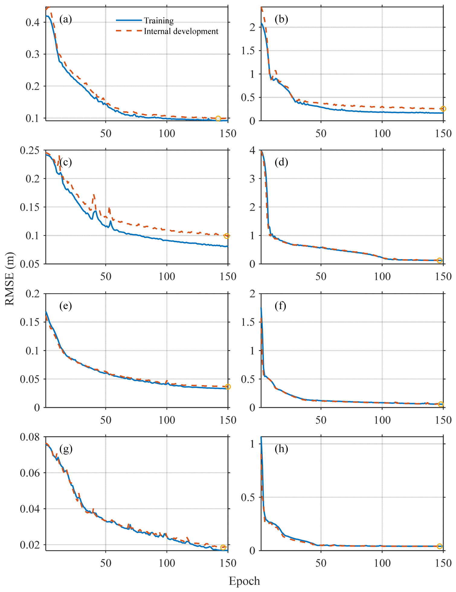
The CNN convolutional layers were initialized using Kaiming-normal initialization with zero biases, while the final output convolution was initialized to zero. The RDN used the default convolutional-layer initialization provided by PyTorch v2.11.0 without additional custom initialization. Both models were trained using the Adam optimizer with an initial learning rate of 1 × 10⁻⁴, a batch size of 16, and a maximum of 150 epochs. Within the training-patch set of each lake, 20% of the patches were reserved as an internal development subset using a fixed partitioning seed of 42. This subset was used for learning-rate scheduling, model selection, and early stopping, but was not included in the external accuracy assessment. The learning rate was reduced by a factor of 0.5 when the internal loss did not improve for six consecutive epochs, and training was stopped after 20 consecutive epochs without improvement in either the internal loss or RMSE. No automated hyperparameter search was conducted for CNN or RDN. The architectures of the CNN and RDN models are illustrated in Figure A1 and Figure A2, respectively, and their principal architecture and training configurations are summarized in

Table 2. Principal architecture and training configurations of the CNN and RDN models.

Configuration	CNN	RDN
Input patch size	32 × 32 × 5	32 × 32 × 5
Number of convolutional layers	11	17
Base channels	64	64
Trainable parameters	317,121	369,281
Optimizer	Adam	Adam
Initial learning rate	1 × 10−4	1 × 10−4
Batch size	16	16
Maximum epochs	150	150
Loss function	Masked Charbonnier loss	Masked Charbonnier loss
Learning-rate adjustment	ReduceLROnPlateau	ReduceLROnPlateau

. The network architectures and training settings were fixed before external validation and applied unchanged to all four lakes. The internal development subset was used for learning-rate scheduling, model selection, and early stopping, whereas the external validation subset was not used for hyperparameter adjustment. The training and internal-development RMSE curves of CNN and RDN using training seed 42 are presented in Figure A3.

Each lake-specific CNN and RDN model was trained using three random seeds (42, 123, and 2026). The training and validation samples, internal development partition, CatBoost-derived initial-depth prior, network architecture, and hyperparameters were held constant across the three runs. The random seed controlled the network initialization, mini-batch ordering, and stochastic data augmentation. The resulting performance was summarized using the mean and standard deviation of the three runs.

Because the ICESat-2-derived reference-depth labels were spatially sparse, a binary validity mask was generated for each training patch. Pixels containing valid reference-depth labels were assigned $M_i=1$, whereas unlabeled pixels were assigned $M_i=0$. The supervised loss was defined using the masked Charbonnier function:

$$L_{\mathrm{c}\mathrm{h}\mathrm{a}\mathrm{r}}={\displaystyle \frac{{\displaystyle {\sum }_{i=1}^N}{M}_i\sqrt{{\left({\widehat{d}}_i-d_i\right)}^2+{\epsilon }^2}}{{\displaystyle {\sum }_{i=1}^N}{M}_i}}$$

(8)

where ${\widehat{d}}_i$ and $d_i$ denote the predicted and ICESat-2-derived reference depths of pixel $i$, respectively; $N$ is the total number of pixels in a mini-batch; and $\epsilon$ was set to ${10}^{-3}$. The loss was normalized by the number of valid labeled pixels, and unlabeled pixels did not contribute to the loss or gradient calculation.

To evaluate the influence of the CatBoost prior-construction strategy on the subsequent deep-learning retrieval, a five-fold out-of-fold (OOF) prior experiment was conducted within the training subset of each lake. For each fold, the CatBoost-derived initial-depth prior corresponding to the held-out spatial blocks was generated using the remaining four folds. The fold-specific priors were then used for CNN and RDN training, ensuring that each supervised depth label was paired with a prior generated without using that label. The external validation samples, network architectures, and other training settings were kept unchanged.

Using the same training and validation settings, additional ablation experiments were conducted to isolate the respective contributions of the CatBoost-derived depth prior and the principal RDN modules. The empirical and CatBoost models provided multispectral-only baselines because both models were trained directly from Sentinel-2 spectral bands without an external depth prior. The CatBoost prediction was also considered the unrefined prior-only result because it was directly used as the initial-depth input for the subsequent CNN and RDN models. Additional CNN and RDN variants were trained using only the four Sentinel-2 bands after removing the CatBoost-derived depth prior, whereas the complete CNN and RDN represented the combined multispectral-plus-prior configuration. Because the original CNN predicted a bounded residual correction relative to the CatBoost-derived prior, the prior-free CNN retained the same convolutional feature-extraction backbone but directly predicted water depth. For the prior-free RDN, only the CatBoost-derived prior channel was removed, while the remaining network architecture was retained. Two additional RDN variants were constructed by removing either the dense connections within the residual dense blocks or the global feature-fusion module while retaining the remaining input, data-partition, and training settings.

2.7. Validation and Accuracy Assessment

Because independent in situ bathymetric measurements were unavailable for the study area, the ICESat-2-derived depths were treated as reference observations rather than absolute ground truth. Previous studies have reported ICESat-2-derived supraglacial lake depth errors of approximately 0.30–0.50 m under favorable conditions [20,21]. The training and validation depth samples were spatially separated, but both were generated using the same ICESat-2 photon-processing and depth-correction workflow. Accordingly, the reported validation metrics characterize the agreement between the model predictions and the ICESat-2-derived reference depths, rather than validation against an independent bathymetric dataset.

To reduce the influence of spatial autocorrelation among neighboring pixels within the same lake, the samples in each lake were divided into training and validation sets using a spatially blocked sampling strategy. Specifically, the pixel-level samples were grouped into non-overlapping square spatial blocks aligned with the Sentinel-2 image grid, with each block containing 5 × 5 pixels and defined according to the pixel row and column indices. At the 10 m spatial resolution, each block corresponded to an area of approximately 50 m × 50 m. The training and validation samples were split at a target 8:2 ratio. Complete spatial blocks were assigned to either the training or validation subset using a group-wise random partitioning procedure with a fixed random seed of 42, ensuring that all samples within the same block were retained in only one subset. No additional buffer distance was imposed between the training and validation blocks, and spatially adjacent blocks could therefore be assigned to different subsets. Both the training and validation samples were obtained from the same lake. The same external training–validation partitions were used for the empirical model, CatBoost, CNN, and RDN. This strategy retained sufficient samples for model training while ensuring that all labeled pixels within the same spatial block were assigned exclusively to either the training or validation subset. Because the training and validation subsets were constructed separately within each lake, the present evaluation primarily assesses within-lake spatial holdout performance rather than transferability to previously unseen lakes.

Model performance was evaluated using the coefficient of determination $\left(R^2\right)$, root mean square error (RMSE), and mean absolute error (MAE). RMSE is sensitive to large errors and reflects the overall magnitude of prediction errors, whereas MAE measures the average absolute difference between the predicted and reference depths. $R^2$ was used to quantify the ability of the model to explain the spatial variation in water depth. These metrics are defined as follows:

$$R^2=1-{\displaystyle \frac{\sum (h_i-\widehat{h_i}{)}^2}{\sum (h_i-\stackrel{-}{h}{)}^2}}$$

(9)

$$RMSE=\sqrt{{\displaystyle \frac{1}{n}}{\displaystyle \sum _{i=1}^n}(h_i-\widehat{h_i}{)}^2}$$

(10)

$$MAE={\displaystyle \frac{1}{n}}{\displaystyle \sum _{i=1}^n}\mid h_i-\widehat{h_i}\mid$$

(11)

where $h_i$ is the ICESat-2-derived reference depth of the $i$-th validation pixel, ${\widehat{h}}_i$ is the corresponding model-predicted depth, $\overline{h}$ is the mean reference depth of the validation samples, and $n$ is the number of valid validation pixels. To quantify the uncertainty associated with the limited validation samples, 95% confidence intervals for RMSE and MAE were estimated using a spatial-block bootstrap with 2000 resamples. In each bootstrap iteration, the validation blocks within each lake were sampled with replacement, and RMSE and MAE were recalculated using all pixels contained in the selected blocks. For the mean performance across the four lakes, the bootstrap metrics were calculated independently for each lake and then averaged with equal weight across the four lakes. By comparing the $R^2$, RMSE, and MAE values of the empirical model, CatBoost, CNN, and RDN across different lakes, the retrieval accuracy, error magnitude, and stability of each model were assessed. The best-performing model was then selected for generating spatially continuous supraglacial lake depth maps.

To examine whether the overall model ranking was affected by the unequal numbers of validation samples among the four lakes, all external validation pixels were pooled to calculate aggregate $R^2$, RMSE, and MAE values, and lake-wise median metrics were also calculated. Pairwise differences in RMSE and MAE between RDN and the other models were evaluated using two-sided paired spatial-block permutation tests with 100,000 permutations, followed by Holm correction for multiple comparisons.

3. Results

3.1. Photon Filtering and Lake Area Extraction

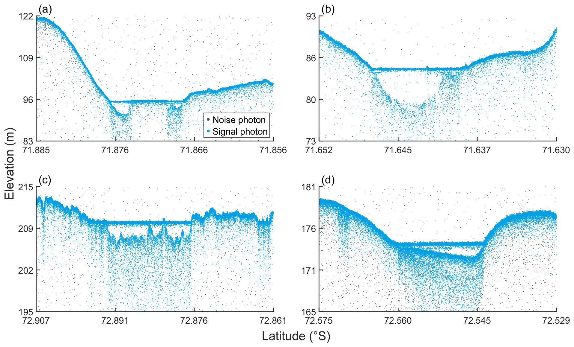
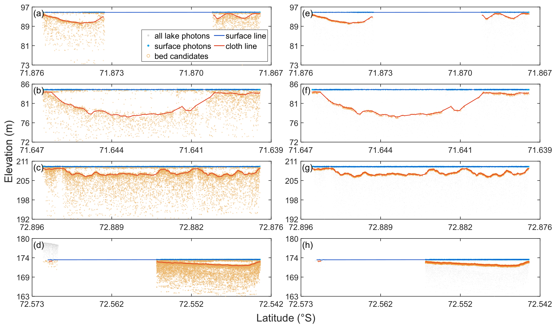
Figure 3 shows investigated examples of signal photon extraction using the PQI method over four supraglacial lakes. After PQI filtering, most background and atmospheric noise photons located far from the surface profile were effectively removed, whereas the main signal photons from the surrounding ice surface, lake surface, and subsurface returns were largely preserved. This result indicates that PQI can provide a reliable initial signal photon set for subsequent lake photon identification. However, several low-elevation photons remain below the apparent lake bottom after filtering. These photons exhibit a downward-extending tail, which is consistent with the scattering signals generated within the water column and lake-bottom ice. Therefore, the PQI-filtered photons were used only as the initial signal photon dataset, and the sub-bottom scattering photons were further corrected during the subsequent construction of ICESat-2 depth samples.

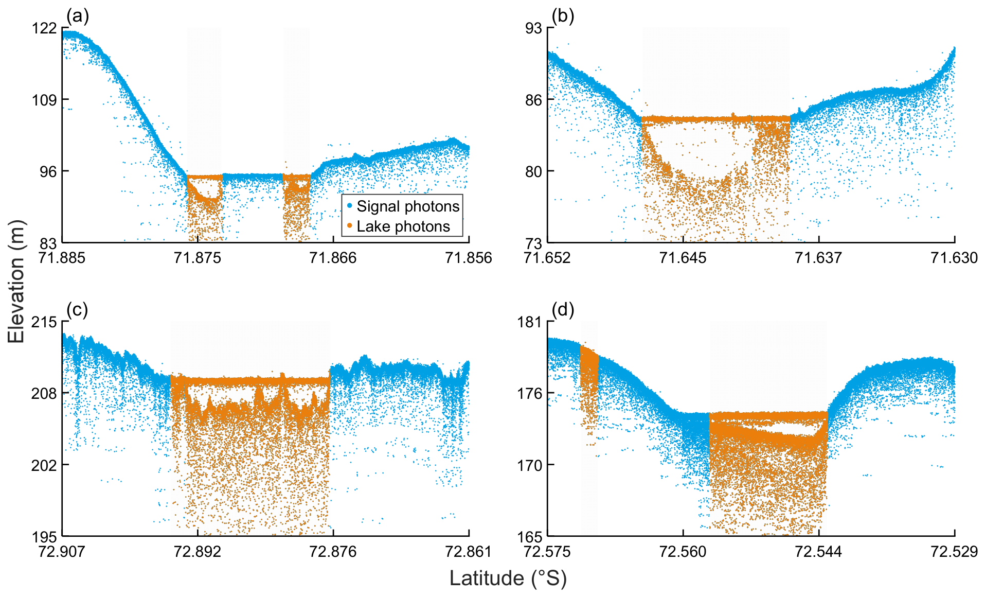
Building on the PQI-filtered signal photons, the PR, STD, and DI metrics were used to identify lake photons along the ICESat-2 ground track. As shown in Figure 4, segments with elevated DI values generally correspond to portions of the photon profile where both lake-surface and subsurface returns are present. This agreement indicates that the DI metric can effectively capture the statistical differences in photon distribution between supraglacial lake areas and the surrounding snow and ice surfaces. For lakes with relatively continuous along-track distributions, the identified lake photons show good spatial completeness. For lakes that are discontinuously intersected by the ICESat-2 track, the method is still able to retain the major lake segments, suggesting that the PR–STD–DI-based identification method has some adaptability to lakes with different spatial forms and along-track distributions.

The identified lake photons were further spatially matched with Sentinel-2 imagery to support lake-region extraction. As shown in Figure 5, the ICESat-2 lake photons are distributed along the satellite ground tracks and intersect the lake areas visible in the Sentinel-2 imagery. The NDWI_ice values of the corresponding Sentinel-2 pixels were extracted and used as observational constraints for determining lake extraction thresholds. 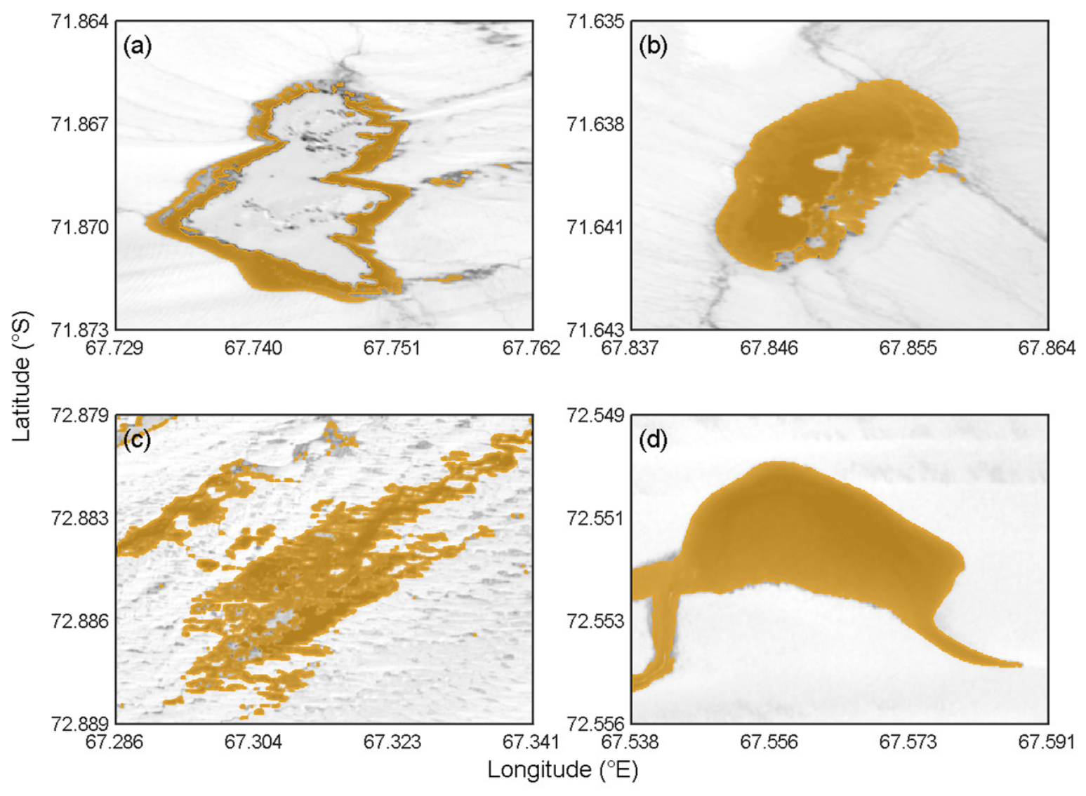Figure 6 presents the extracted lake regions for investigated supraglacial lakes. Overall, the extracted lake masks agree well with the dark-blue water areas visible in the Sentinel-2 images, indicating that ICESat-2 along-track lake photons can provide effective constraints for Sentinel-2-based lake mapping. For lakes with regular shapes and well-defined boundaries, the extracted masks show good spatial continuity. In contrast, lakes with fragmented boundaries or mixed ice–water surfaces exhibit more discontinuous extraction results.

To quantitatively evaluate lake-region extraction, the automatically extracted lake masks were compared with reference masks manually labeled from the same-day Sentinel-2 imagery using IoU, precision, recall, and F1-score. As summarized in

Table 3. Quantitative assessment of the automatically extracted lake masks against manually labeled reference masks.

Lake	IoU	Precision	Recall	F1-Score
Lake 1	0.853	0.967	0.879	0.921
Lake 2	0.978	0.988	0.990	0.989
Lake 3	0.813	0.816	0.977	0.889
Lake 4	0.952	0.994	0.957	0.975

, the automatically extracted lake masks achieved mean IoU, precision, recall, and F1-score values of 0.899, 0.941, 0.951, and 0.944, respectively. Lake 2 and Lake 4 showed the highest agreement with the reference masks, whereas Lake 1 exhibited a relatively lower recall and Lake 3 showed a lower precision. The relatively lower performance for Lakes 1 and 3 was mainly associated with fragmented lake boundaries, spectral similarity between open water and thin ice or wet snow, and mixed pixels along the lake margins.

3.2. ICESat-2 Depth Correction and Label Generation

The identified lake photons were further processed to derive corrected ICESat-2 depth samples. Within each extracted lake region, photons were classified into lake-surface returns, candidate lake-bottom returns, and scattering returns. Because ATL03 photons are affected by scattering and refraction after entering the water column, the raw candidate bottom photons cannot be directly used for depth estimation. Scattering correction and refraction correction were therefore applied before constructing the final depth samples.

Figure 7 compares representative ICESat-2 photon profiles before and after scattering correction. Before correction, numerous low-elevation photons appear below the apparent lake bottom, forming a downward-extending scattering tail. These photons are mainly associated with water-column scattering and scattering within the ice at the lake bed, rather than the actual bottom surface. If such photons are included in bottom fitting, the estimated bottom elevation may be biased downward, leading to an overestimation of water depth. After correction, most sub-bottom scattering photons are suppressed, and the retained bottom photons are more tightly distributed around the fitted bottom profile. The corrected bottom profile also shows improved spatial continuity, indicating that scattering correction provides a more stable basis for subsequent depth estimation.

The effectiveness of scattering correction varies among different lakes. For lakes with a pronounced scattering tail, the vertical spread of candidate bottom photons is substantially reduced after correction. For shallow lakes or lakes with relatively smooth bottom topography, the fitted bottom profile changes only slightly, although locally scattered photons are still removed. This suggests that scattering correction is useful not only for eliminating obvious outliers, but also for reducing the influence of local scattering signals on lake-bottom fitting.

After scattering correction, refraction correction, and pixel matching, the ICESat-2 along-track depth observations were converted into Sentinel-2 pixel-scale reference depth samples. For the four investigated lakes, a total of 8947 photon-level depth observations were obtained after correction. These observations were further aggregated at the Sentinel-2 pixel scale, resulting in 565 valid pixel-level depth labels. Specifically, Lake 1, Lake 2, Lake 3, and Lake 4 contained 57, 87, 237, and 184 pixel-level depth labels, respectively. The sampled reference depths ranged from 0.388 to 3.488 m in Lake 1, from 0.389 to 5.102 m in Lake 2, from 0.342 to 2.664 m in Lake 3, and from 0.171 to 1.509 m in Lake 4. The corresponding mean depths were 1.851, 2.978, 1.642, and 1.011 m, respectively. Among the four lakes, Lake 2 exhibited the widest sampled depth range and the highest mean depth, whereas Lake 4 showed the narrowest depth range and the lowest mean depth.

Of the 565 pixel-level depth labels, 536 (94.9%) contained at least two corrected photon-depth observations and were included in the bootstrap analysis, whereas 29 (5.1%) were single-photon labels. The median pixel-level sampling uncertainties were 0.036, 0.046, 0.035, and 0.023 m for Lakes 1–4, respectively. The corresponding interquartile ranges were 0.027–0.053, 0.033–0.060, 0.030–0.044, and 0.019–0.026 m, while the median widths of the 95% confidence intervals were 0.141, 0.177, 0.137, and 0.088 m, respectively.

3.3. Bathymetry Retrieval Performance

Based on the constructed ICESat-2 pixel-level reference depth samples, the four investigated supraglacial lakes were used to evaluate the performance of the empirical model, CatBoost, CNN, and RDN.

Table 4. Accuracy assessment of lake depth retrieval using different models. Values in parentheses are 95% confidence intervals derived from spatial-block bootstrap resampling.

Lake	Model	R2	RMSE (m; 95% CI)	MAE (m; 95% CI)
Lake 1	Empirical	0.746	0.504 (0.295–0.879)	0.412 (0.269–0.877)
	CatBoost	0.775	0.474 (0.208–0.868)	0.305 (0.138–0.748)
	CNN	0.773	0.477 (0.207–0.872)	0.309 (0.143–0.746)
	RDN	0.917	0.289 (0.147–0.421)	0.216 (0.119–0.336)
Lake 2	Empirical	0.974	0.249 (0.146–0.315)	0.213 (0.114–0.302)
	CatBoost	0.983	0.204 (0.116–0.332)	0.159 (0.105–0.280)
	CNN	0.980	0.219 (0.120–0.368)	0.168 (0.106–0.297)
	RDN	0.981	0.214 (0.117–0.330)	0.164 (0.108–0.271)
Lake 3	Empirical	0.890	0.166 (0.121–0.211)	0.135 (0.097–0.180)
	CatBoost	0.874	0.178 (0.133–0.227)	0.140 (0.106–0.182)
	CNN	0.885	0.170 (0.130–0.210)	0.134 (0.104–0.167)
	RDN	0.857	0.189 (0.136–0.241)	0.151 (0.113–0.196)
Lake 4	Empirical	0.939	0.067 (0.058–0.074)	0.056 (0.045–0.066)
	CatBoost	0.961	0.053 (0.041–0.064)	0.044 (0.034–0.055)
	CNN	0.931	0.071 (0.050–0.088)	0.056 (0.041–0.070)
	RDN	0.955	0.058 (0.044–0.073)	0.046 (0.036–0.060)

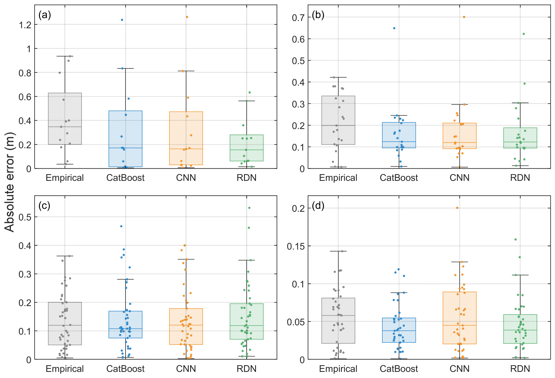
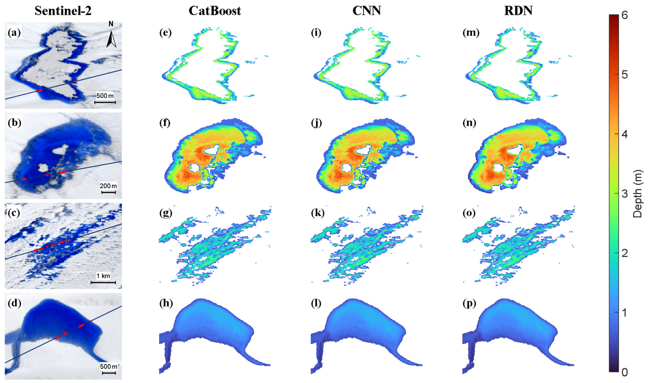
reports the corresponding $R^2$, RMSE, and MAE values for each model and lake. Figure 8 presents the distributions of absolute errors at the validation pixels, whereas Figure 9 shows the spatial bathymetry results generated by CatBoost, CNN, and RDN.

Figure 8 shows that the absolute-error distributions varied among the four lakes. For Lake 1, RDN exhibited the lowest median absolute error and a relatively compact error distribution, whereas the empirical model showed larger errors. For Lake 2, CatBoost, CNN, and RDN produced similar median errors and interquartile ranges, all of which were lower than those of the empirical model. For Lake 3, the median errors of the four models were relatively similar, although RDN showed a wider upper error range. For Lake 4, all four models produced small absolute errors, with CatBoost and RDN exhibiting comparatively compact distributions. These error-distribution characteristics were generally consistent with the R², RMSE, and MAE results reported in Table 4.

The spatial-block bootstrap confidence intervals for the lake-specific RMSE and MAE values are reported in Table 4. Based on the equal-weighted mean across the four lakes, RDN achieved the highest mean $R^2$ and the lowest mean RMSE and MAE, with values of 0.927, 0.187 m, and 0.144 m, respectively. Compared with CatBoost, RDN reduced the mean RMSE and MAE by approximately 17.6% and 10.8%, respectively; compared with CNN, the corresponding reductions were approximately 20.0% and 13.4%.

To account for the unequal numbers of validation samples among the lakes, all 113 external validation pixels were pooled for an aggregate assessment. The pooled $R^2$, RMSE, and MAE values were 0.935, 0.229 m, and 0.155 m for the empirical model; 0.943, 0.215 m, and 0.131 m for CatBoost; 0.941, 0.218 m, and 0.135 m for CNN; and 0.960, 0.180 m, and 0.127 m for RDN, respectively. RDN therefore retained the highest pooled $R^2$ and the lowest pooled RMSE and MAE after the unequal validation sample sizes were taken into account.

The lake-wise median analysis showed that RDN achieved the highest median $R^2$ of 0.936, whereas CatBoost achieved the lowest median RMSE and MAE values of 0.191 m and 0.149 m, respectively. Overall, RDN achieved the best equal-weighted average performance and the most favorable pooled metrics across the four investigated lakes, while the relative model rankings varied among individual lakes. The paired spatial-block permutation tests did not detect statistically significant pairwise differences after Holm correction under the current validation-block sample.

The ablation experiments further clarified the contributions of the input components and RDN structural modules. Because CatBoost was trained only from the four Sentinel-2 bands and its output was directly used as the initial-depth prior, the CatBoost result represented both a nonlinear multispectral-only baseline and the unrefined prior-only condition. It achieved four-lake mean R², RMSE, and MAE values of 0.898, 0.227 m, and 0.162 m, respectively. When the CatBoost-derived prior was removed from the deep-learning models, the mean RMSE increased to 1.216 m for CNN and 1.120 m for RDN, while the corresponding mean MAE values increased to 0.996 m and 0.908 m. In comparison, combining the multispectral bands with the CatBoost prior resulted in mean RMSE values of 0.234 m for CNN and 0.187 m for RDN. Removing the dense connections from RDN increased the mean RMSE and MAE to 0.233 m and 0.177 m, respectively. Removing global feature fusion produced only minor and metric-dependent changes, with a mean RMSE of 0.190 m and a mean MAE of 0.138 m.

As summarized in

Table A1. Five-fold OOF-prior evaluation results for CNN and RDN over the four investigated lakes.

Lake	Model	R2	RMSE (m)	MAE (m)
Lake 1	CNN	0.790	0.458	0.290
	RDN	0.787	0.462	0.399
Lake 2	CNN	0.981	0.216	0.158
	RDN	0.973	0.253	0.209
Lake 3	CNN	0.818	0.214	0.165
	RDN	0.816	0.215	0.160
Lake 4	CNN	0.933	0.070	0.055
	RDN	0.946	0.063	0.053

, the five-fold OOF-prior experiment was performed using the same external validation samples as the main experiment. Under the OOF-prior setting, CNN achieved four-lake mean R², RMSE, and MAE values of 0.881, 0.239 m, and 0.167 m, respectively, while the corresponding values for RDN were 0.880, 0.248 m, and 0.205 m. Both networks retained effective bathymetry-retrieval capability across the four investigated lakes. The CNN results were close to those obtained in the main experiment, whereas the response of RDN varied more among lakes, indicating differences between the two network architectures in their integration of the CatBoost-derived initial-depth prior.

As summarized in

Table A2. Performance of CNN and RDN across three training runs. Values are reported as mean ± standard deviation.

Lake	Model	R2	RMSE (m)	MAE (m)
Lake 1	CNN	0.778 ± 0.005	0.471 ± 0.005	0.306 ± 0.006
	RDN	0.911 ± 0.017	0.297 ± 0.027	0.223 ± 0.013
Lake 2	CNN	0.980 ± 0.001	0.221 ± 0.003	0.171 ± 0.003
	RDN	0.976 ± 0.004	0.240 ± 0.022	0.180 ± 0.015
Lake 3	CNN	0.879 ± 0.006	0.174 ± 0.005	0.138 ± 0.005
	RDN	0.876 ± 0.027	0.175 ± 0.020	0.137 ± 0.021
Lake 4	CNN	0.938 ± 0.008	0.067 ± 0.004	0.053 ± 0.003
	RDN	0.963 ± 0.007	0.052 ± 0.005	0.042 ± 0.003

, the three-run results showed limited variability in the retrieval performance of both deep-learning models. The standard deviations of the CNN RMSE values ranged from 0.003 to 0.005 m across the four lakes, whereas those of RDN ranged from 0.005 to 0.027 m. CNN therefore exhibited smaller between-run variation, while RDN retained lower mean RMSE and MAE values for Lakes 1 and 4 across the three runs. As shown in Figure A3, the training and internal-development RMSE values generally decreased and stabilized toward the later epochs, although the convergence patterns varied among lakes and between the two network architectures.

3.4. Spatial Bathymetry Results

The spatial retrieval results in Figure 9 are generally consistent with the quantitative assessment. CatBoost, CNN, and RDN can all capture the main spatial patterns of lake depth, but differences remain in local continuity and detail representation. For Lake 1, comparison of Figure 9e,i,m shows that all three models identify the shallow marginal regions and the main lake body. However, the CatBoost and CNN results contain more fragmented local pixel variations, whereas the RDN result maintains a more coherent depth pattern and fewer local fluctuations, consistent with its lowest RMSE and MAE in Table 4. For Lake 2, Figure 9f,j,n all show a clear deep-water center and a gradual shallowing pattern toward the lake margins. The three models show relatively small spatial differences, and the CatBoost and RDN results are particularly similar. For Lake 3, the retrieved depth patterns in Figure 9g,k,o are relatively fragmented, and the spatial results of the three models are generally similar. For Lake 4, Figure 9h,l,p show that all three models preserve the overall lake shape and continuous depth variation. The spatial distributions from CatBoost and RDN are relatively consistent, whereas CNN produces a smoother result and shows weaker representation of local depth details.

4. Discussion

4.1. Model Performance and Ablation Analysis

Overall, the quantitative and spatial comparisons demonstrate the effectiveness of the proposed retrieval strategy. Among the four models, RDN achieved the best average performance across the four investigated lakes, with the highest mean R² and the lowest mean RMSE and MAE. Its performance improvement was most evident for Lake 1, where the depth distribution showed stronger spatial variability, suggesting that residual dense feature learning is effective in representing complex and spatially heterogeneous lake-depth patterns. The spatial retrieval maps further support this result: compared with CatBoost and CNN, RDN produced more coherent depth distributions with fewer fragmented local fluctuations, while CNN showed only limited improvement over the CatBoost-derived initial estimates and tended to smooth local depth details.

The lake-specific spatial patterns also help explain the variation in model performance. For Lake 2, the similarity among the CatBoost, CNN, and RDN results may reflect a relatively stable relationship between multispectral reflectance and water depth. In contrast, the fragmented retrieval patterns for Lake 3 may be associated with its discontinuous lake boundary, complex morphology, and dispersed valid lake pixels. Under these shallow and spatially fragmented conditions, the advantage of a more complex deep-learning model was not evident.

The lake-by-lake results further show that the applicability of different models depends on the internal depth variation of each lake and the complexity of the spectral–depth relationship. The performance improvement of RDN was most evident for Lake 1. In this lake, RDN achieved an R² of 0.917 and reduced the RMSE and MAE to 0.289 m and 0.216 m, respectively, indicating a stronger ability to represent spatially variable depth patterns. For Lake 2, CatBoost, CNN, and RDN all achieved high accuracy. CatBoost obtained the highest R² of 0.983, with an RMSE of 0.204 m and an MAE of 0.159 m, while RDN produced comparable results, with an R² of 0.981, an RMSE of 0.214 m, and an MAE of 0.164 m. For Lake 3, the empirical model and CNN slightly outperformed CatBoost and RDN, suggesting that simpler models can still provide stable results when the depth variation is relatively smooth or when the spectral–depth relationship is less complex. For Lake 4, CatBoost showed the best performance, with an R² of 0.961, an RMSE of 0.053 m, and an MAE of 0.044 m. The RDN result was close to that of CatBoost, indicating that CatBoost can already provide reliable initial depth estimates for shallow lakes with relatively clear spectral responses.

The ablation results indicate that the CatBoost-derived initial-depth prior was the principal factor supporting stable spatial generalization of the deep-learning models under the available sparse-label conditions. Although the empirical and CatBoost models demonstrated that the selected Sentinel-2 bands contained useful depth-related information, CNN and RDN trained without the initial-depth prior showed substantial performance deterioration. The CatBoost prior therefore provided an important constraint on the approximate depth range, while the subsequent spatial networks refined the initial estimates using local multispectral patterns. Among the RDN modules, removing dense connections reduced the overall accuracy, supporting the role of dense feature propagation and reuse. In contrast, removing global feature fusion caused only small and metric-dependent changes, suggesting that this module did not provide a consistent independent improvement for all investigated lakes. Therefore, the overall performance of RDN is more appropriately attributed to the combination of a stable CatBoost-derived prior and residual dense spatial refinement, rather than to a uniform contribution from every individual architectural component.

The OOF-prior experiment further clarifies the interaction between the CatBoost-derived initial-depth prior and the subsequent deep-learning refinement. Compared with the main configuration, the four-lake mean RMSE of CNN changed only slightly from 0.234 to 0.239 m under the OOF-prior setting, whereas that of RDN changed from 0.187 to 0.248 m. Both networks nevertheless retained effective bathymetry-retrieval capability, indicating that the two-stage framework remained functional when each supervised training label was paired with a prior generated without using that label. The larger response of RDN suggests that its residual dense reconstruction makes more intensive use of the detailed information contained in the initial-depth field during spectral–spatial refinement. Together with the ablation results, this finding highlights the complementary roles of the two stages: CatBoost provides a stable pixel-level spectral depth constraint, while RDN further integrates this prior with neighborhood spectral–spatial information to refine the bathymetric field. The favorable performance of the complete RDN configuration therefore reflects the coordinated contribution of the CatBoost-derived initial-depth prior and the residual dense refinement architecture.

4.2. Uncertainty and Validation Limitations

Because ICESat-2 provides along-track observations, the aggregated pixel-level depth labels are mainly distributed within lake pixels intersected by the satellite ground tracks. These labels are spatially discrete but have relatively high depth reliability. They cannot directly form continuous lake bathymetry maps, but they establish the correspondence between corrected ICESat-2 depths and Sentinel-2 pixel-level spectral features. Therefore, they provide the supervised reference information required for subsequent bathymetry retrieval models, allowing the discrete along-track depth samples to be extended to spatially continuous lake depth predictions using Sentinel-2 imagery.

The training labels and evaluation references were produced using the same ICESat-2 photon-processing and depth-correction workflow. Although the spatially blocked partition prevented the same depth samples from being included in both the training and evaluation subsets, the evaluation was not independent of uncertainties associated with label generation. Potential uncertainty sources include signal-photon filtering, lake-surface and lake-bottom identification, scattering correction, refraction correction, and the aggregation of photon-level depths to Sentinel-2 pixels. These uncertainties may propagate into the pixel-level reference-depth labels and subsequently affect model fitting and the reported evaluation metrics. The bootstrap analysis provided a quantitative estimate of the random uncertainty associated with corrected-photon sampling and pixel-level aggregation. However, this analysis does not represent absolute bathymetric accuracy and does not include systematic errors that may be shared by the corrected photon depths, such as residual biases associated with photon classification, lake-bottom fitting, scattering correction, and refraction modeling. Accordingly, the reported metrics provide a measure of consistency with the ICESat-2-derived reference depths under the investigated conditions. Independent bathymetric observations are still required to assess absolute retrieval accuracy.

4.3. Applicability and Future Work

The present evaluation was limited to four investigated lakes on the Amery Ice Shelf and 565 pixel-level depth labels, and therefore covered a restricted range of lake morphology, depth distribution, optical properties, and photon-sampling conditions. Because the training and validation samples were obtained from the same lake scenes, the reported results primarily characterize within-lake spatial generalization under the investigated conditions rather than transferability to unseen lakes. Because no buffer zone was imposed between adjacent training and validation blocks and the 32 × 32-pixel input patches were larger than the 5 × 5-pixel spatial blocks, some overlap in the surrounding image context may have remained near the block boundaries. Although the external validation depth labels were fully excluded from model training, neighboring training and validation regions may still share part of their local Sentinel-2 spectral–spatial context. Therefore, the current validation is most appropriately interpreted as an assessment of within-lake spatial generalization, while the remaining contextual overlap should be considered when extending the evaluation to more strictly independent spatial settings. Future studies using larger reference datasets should further assess model robustness through repeated spatial partitions with explicit buffer zones.

The framework is expected to be most reliable when sufficient ICESat-2 lake-surface and lake-bottom photons are available, the Sentinel-2 lake pixels exhibit relatively consistent spectral responses with limited thin-ice and mixed-pixel effects, and the available training samples cover the lake’s depth range and spectral variability. Performance may be less stable for lakes with sparse or discontinuous bottom-photon returns, complex or fragmented boundaries, extensive thin-ice cover, strong mixed-pixel effects, or spectral and depth conditions outside the training range. Transferability to unseen lakes, other ice shelves, and different observation periods remains to be evaluated.

Future work should incorporate independent field or otherwise independently derived bathymetric observations, together with additional lakes covering diverse optical and geomorphological conditions, to assess the absolute accuracy, robustness, and transferability of the proposed framework.

5. Conclusions

This study developed an integrated ICESat-2/Sentinel-2 framework for supraglacial lake identification and bathymetry retrieval and evaluated it over four investigated lakes on the Amery Ice Shelf. In this framework, ICESat-2 ATL03 photon data were processed to identify lake photons and derive corrected along-track depth observations. Sentinel-2 multispectral imagery provided spatially continuous information on lake extent and spectral characteristics. The corrected ICESat-2-derived depths were matched with Sentinel-2 pixels to generate pixel-level depth labels for model training and validation.

The constructed pixel-level labels were used to train and validate four bathymetry retrieval models over four investigated supraglacial lakes, including an empirical model, CatBoost, CNN, and RDN. RDN achieved the best average performance across the four investigated lakes, with mean R², RMSE, and MAE values of 0.927, 0.187 m, and 0.144 m, respectively. However, the relative model rankings remained lake-dependent, with CatBoost performing best for Lakes 2 and 4 and the empirical model or CNN remaining competitive for Lake 3. The paired spatial-block permutation tests did not detect statistically significant pairwise differences after Holm correction under the current validation-block sample. CatBoost provided a stable initial depth estimate under limited sample conditions. CNN incorporated local spatial information, but its improvement over CatBoost was limited. RDN integrated the CatBoost-derived initial depth prior with Sentinel-2 multispectral and spatial features, producing the best average accuracy and spatially coherent bathymetry retrieval results across the investigated lakes.

Across the four investigated lakes, the proposed framework extended discrete ICESat-2 along-track depth observations to spatially continuous supraglacial lake bathymetry maps, which may provide bathymetric inputs for future meltwater storage estimation and ice-shelf hydrological analysis. However, the retrieval accuracy is still influenced by the spatial distribution of ICESat-2 samples and the complexity of lake optical conditions, including lake-region extraction uncertainty, thin ice cover, mixed pixels, and variations in lake-bottom reflectance. Because the present evaluation was conducted on four investigated lakes using training and validation samples from the same lake scenes, the reported results primarily characterize within-lake spatial generalization rather than transferability to unseen lakes. Future work should incorporate more supraglacial lakes, multi-temporal observations, and independent validation data to evaluate the robustness and transferability of the framework beyond the investigated lakes and observation conditions.