A Photogrammetric Simulation Framework for Rockfall Change Detection with Statistically Validated Measurement Noise

Highlights

What are the main findings?

• A simulator has been developed to generate 2.5D/3D models of rock faces undergoing rockfall events, modelling the measurement noise affecting the reconstructed geometry and providing objective ground truth (removed rock blocks).
• A multi-indicator validation methodology is proposed to calibrate noise levels and to assess the stochastic compatibility between real and simulated measurement noise.

What are the implications of the main findings?

• The proposed methodology enables reproducible “realistic” simulations of rock detachments, even though measurement-noise characteristics strongly depend on acquisition geometry and on the morphology of the monitored surface.
• The simulator enables a wide range of benchmarking applications for change detection algorithms and supports the generation of reliable ground truth for training machine-learning-based methods.

Abstract

Rockfalls are natural slope-instability phenomena that pose a significant hazard to infrastructure and human activity. In recent years, the increasing availability of high-resolution three-dimensional (3D) models acquired through photogrammetric techniques has enabled detailed pre-/post-event analyses of rock slopes. However, in this domain, the availability of accurate ground truth for the quantitative evaluation of 3D change detection methods and for training machine-learning approaches aimed at recognising and volumetrically quantifying detachments on rock faces remains very limited. This work presents a simulator that, starting from a 3D model of a rock face, generates pre-/post-failure scenarios through controlled removal of rock blocks and produces photogrammetric acquisitions affected by realistic measurement noise. The pipeline emulates the main processing stages of the reconstruction workflow. Noise realism is validated and calibrated by comparing real and simulated data through a multi-indicator framework (marginal distribution, variogram, power spectrum, and multiscale roughness), integrated into a Mahalanobis-distance-based acceptance test with empirical thresholds derived from real measurements. Results from two pilot sites show that, after site-specific tuning of the simulator noise levels, the calibrated configurations reproduce the main magnitude and spatial-structure characteristics of the real noise, with stronger agreement for the fixed stereo-pair configuration and partial but still informative agreement for the more complex UAV-based case. Moreover, the simulator provides a controlled environment for benchmarking and sensitivity analyses of change detection methods.

1. Introduction

Rockfalls are natural slope-instability phenomena that pose a significant hazard to infrastructure and human activity along major transportation corridors, mountain and coastal paths, and underground and surface explorations. Quantitative characterization of rockfall events (i.e., the localization of detachment location, block dimensions, and volume loss) is essential for risk assessment and for designing effective mitigation measures. In recent years, the increasing availability of high-resolution three-dimensional (3D) models acquired through photogrammetric techniques (Structure from Motion, SfM; Multi-View Stereo, MVS) and Light Detection and Ranging (LiDAR) has enabled detailed temporal analyses (pre-/post-event) of rock cliff surfaces [1,2,3,4,5]. This development has opened the way to 3D change-detection procedures, either manual or automated, aimed at identifying and quantifying detached blocks [6,7,8].

However, the accuracy of such analyses is often limited by two key factors: (i) the quality and statistical properties of 3D reconstructions such as noise, occlusions, spatial density, and registration errors (sometimes small rigid or non-rigid misalignments can cause far more false positives than pointwise sensor noise), which strongly affect the detectability and measurability of rockfalls, especially when dealing with small block sizes; and (ii) the difficulty of acquiring accurate and sufficiently extensive ground truth to validate detection procedures and to assess their ability to produce reliable information on susceptibility and risk.

Recently, in many application domains (and only marginally in the field addressed here), automatic detection methods based on Machine Learning (ML) are increasingly proposed (e.g., in refs. [9,10,11]). These methods, however, rely on training phases that critically depend (to varying degrees depending on the ML approach) on large, reliable, and realistic sets of ground truth (GT) data. Obtaining such information, whether to validate change-detection procedures under varying 3D model quality conditions or to generate training datasets, is currently one of the major challenges to developing and deploying automated approaches for rockfall analysis. At present, validation of block-detachment mapping is typically performed manually by expert operators who visually compare pre- and post-event models and verify if corresponding surface changes—previously identified via automatic/semi-automatic change detection algorithms—on the rock wall represent real rockfall events. During this process, human operators benefit from the ability to jointly consider multiple heterogeneous sources and complex interrelated factors, thus reducing false positives: for example, an operator can recognize vegetation on the rock face, identify artefacts caused by misalignment or imperfect georeferencing of the models, use additional information (e.g., imagery, older 3D surveys, acquisition metadata), assess areas affected by outliers or elevated uncertainty, and critically apply geotechnical reasoning to evaluate the plausibility of potential detachment areas. From this perspective, human-interpreted GT appears to be the gold standard for validation, benchmarking, and ML training.

Nevertheless, such GT suffers from two fundamental limitations: (i) a non-negligible degree of subjectivity, heavily dependent on the operator’s expertise and familiarity with 3D comparison procedures; and (ii) the substantial time and resources required to perform a complete and reliable mapping of rockfalls, an effort rarely sustainable in typical real-world scenarios. The former drawback implies that, in practice, human GT itself can be noisy/biased, since inter-annotator variability, bias from training/experience, and systematic tendencies (e.g., conservative vs. aggressive marking) all affect labels. The consequence of the latter limitation is that, at the present time, only a few manually annotated datasets exist, each produced as part of highly focused research projects where substantial resources were specifically allocated [9,10,11].

In this context, the ability to generate synthetic datasets (i.e., obtained by virtually removing blocks from pre-event models and simulating realistic 3D acquisitions with sensor-specific noise) would represent a crucial resource. Such datasets would provide perfect labels (location, extent, shape and volume of removed blocks) and would enable controlled studies on how measurement artefacts affect the capability of change-detection methods to distinguish true detachments from noise, occlusions, or registration inaccuracies, supporting controlled comparative evaluations, sensitivity analyses, and ablation studies that are difficult to conduct using real data alone. However, the simulated data must reproduce the statistical characteristics of the measurement technique being emulated. This study introduces a photogrammetric simulation framework that jointly reproduces rockfall geometry, ground-truth changes, and statistically validated measurement noise, enabling realistic synthetic datasets for benchmarking and algorithm development.

Over the past decade, the systematic production of synthetic datasets with perfect ground truth has become standard practice in many fields of computer vision, robotics, and applied sciences. In domains where manual annotation is costly or infeasible (e.g., 3D semantic segmentation, pose estimation, depth map generation, rare anomalies), synthetic data enables the creation of large-scale datasets with arbitrarily precise and repeatable labels [12]. This trend has been adopted across highly diverse contexts, from autonomous driving simulators such as CARLA [13] and AirSim [14] to robotic manipulation [15], industrial inspection [16], and medical imaging [17]. As a result, a broad literature has emerged on synthetic-data generation (3D rendering, neural rendering, Generative Adversarial Networks (GANs), diffusion models, etc.) and on best practices for integrating synthetic data into benchmarking and ML training pipelines.

In the specific domain addressed in this study (i.e., synthetic 4D scenes with rockfall/landslide events and simulated point clouds for benchmarking or ML training), only a few recent works exist [18,19,20]. In the rockfall domain, simulation approaches have also been used to reproduce fragmental rockfall runout from TLS-derived source geometries and change-detection inventories, for example through game-engine-based 3D simulations of multiple interacting fragments [21]. However, such works primarily address post-detachment dynamics and runout, whereas the present study focuses on generating controlled pre-/post-failure geometries for change-detection benchmarking. This scarcity is likely due not only to the niche nature of rockfall monitoring compared to more general applications (e.g., urban change detection, robotics, image segmentation, point-cloud classification), but also to the numerous implementation choices required to simulate realistic SfM or Terrestrial Laser Scanning (TLS) acquisitions (ray tracing, sensor-specific noise models, 3D registration, etc.). Moreover, much of the scientific community’s effort is currently oriented toward practical tools and ready-to-use datasets (e.g., HELIOS++ [22], 3D and 4D benchmarking datasets [23]), rather than toward methodological developments tailored to specific application domains.

Across a broader application spectrum, several fields, including robotics, cultural-heritage documentation, and urban or infrastructure monitoring, have successfully employed synthetic data pipelines for semantic segmentation or 3D change detection [24]. For example, in ref. [25] the authors use 3D building models to generate labelled synthetic point clouds for training a modified DGCNN (Dynamic Graph Convolutional Neural Network) for semantic segmentation. Esmorís et al. [26] demonstrate that a deep-learning classifier trained solely on virtual LiDAR data can generalize effectively to real-world point clouds, with only minor accuracy losses compared to models trained directly on real acquisitions. In the context of 3D change detection, de Gélis et al. [27] generate an artificial urban environment, simulating multiple temporal epochs of point clouds from a CityGML-derived mesh, where buildings are added or removed with corresponding perfect ground-truth labels. Classical methods (Cloud-to-Cloud—C2C, Multiscale Model-to-Model Cloud Comparison—M3C2 [6,28]), ML classifiers using hand-crafted features and deep networks operating on rasterized Digital Surface Model (DSM) representations or directly on 3D point clouds were benchmarked on this dataset [27]; results show that even with noise-free data, none of the approaches reaches perfect performance, highlighting the intrinsic complexity of the task. However, the practical usefulness of synthetic data is not guaranteed: the core challenge is the so-called reality gap (or sim-to-real gap) [29,30], namely the discrepancy between the statistical properties of simulated data and those of real-world acquisitions. Reducing this gap, measuring it [31], and understanding its impact on downstream tasks are today essential research directions for ensuring that synthetic datasets provide meaningful value [32]. Several studies have demonstrated measurable impacts of the gap, e.g., performance drops of LiDAR detectors by around ten percentage points when moving from simulated to real data, and have proposed different mitigation strategies, including domain randomization, domain adaptation, noise calibration, and hybrid compositing.

This study presents a simulation framework based on synthetic photogrammetric data to address a key limitation of real-world rockfall monitoring, namely the lack of fully known GT and the presence of unavoidable measurement noise. In photogrammetric surveys, change detection is widely used to identify and quantify rockfall events. However, real data does not allow true surface change to be clearly separated from errors introduced during image acquisition and 3D reconstruction. By generating controlled rockfall scenarios from a known reference model, the proposed simulator provides a reproducible environment for evaluating the performance of photogrammetric change detection under different acquisition and noise conditions.

2. Materials and Methods

2.1. Simulation Framework for Rockfall Change Detection

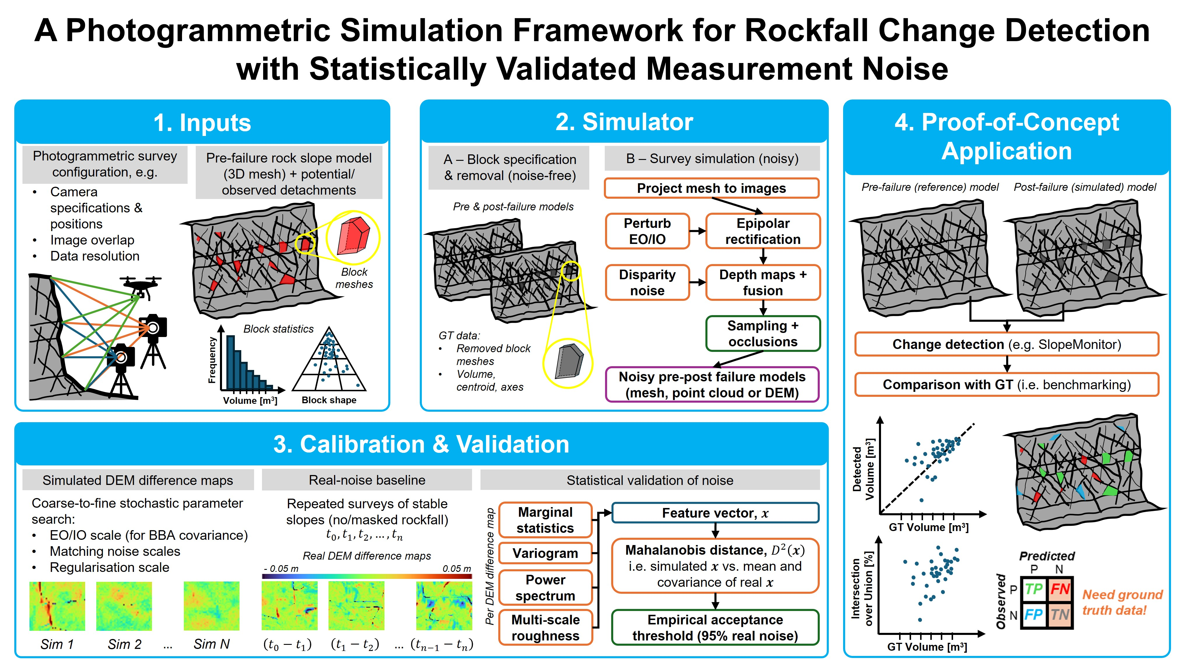
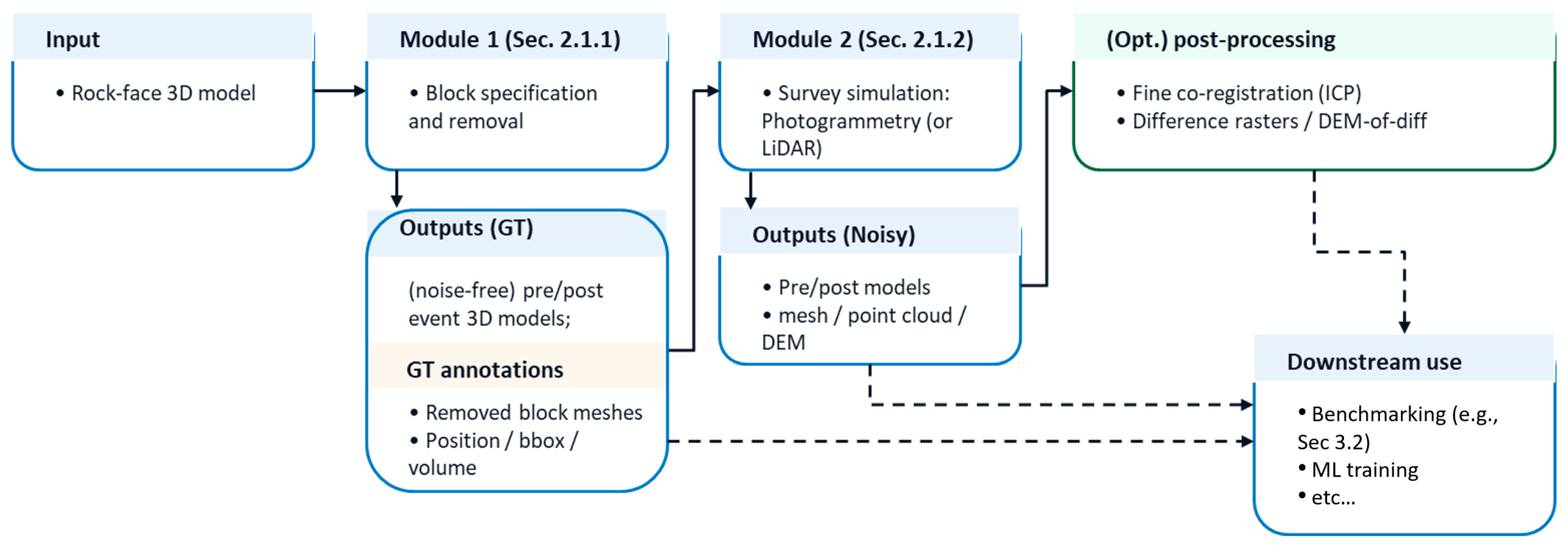
This section presents the developed simulation methodology. Starting from a 3D digital model of a rock cliff, the proposed framework virtually reproduces a series of detachment events and emulates the data acquisition process as if it is performed by a real monitoring system. The software architecture was designed to be extensible to different acquisition techniques (e.g., either a photogrammetric or LiDAR acquisition); however, the present work implements, calibrates, and validates only the photogrammetric branch of the framework. LiDAR simulation is therefore outside the scope of this paper. The simulator reproduces the main sources of measurement noise affecting the observations, and provides all the information required to automate both the benchmarking of change detection algorithms and the training of ML-based approaches (Figure 1).

The simulator is composed of two modules executed sequentially. The first module (Section 2.1.1), starting from the undisturbed (error-free) digital model of the rock face, simulates detachment events by removing a set of rock blocks, effectively reshaping the surface. The shape, size, and spatial location of these blocks can either be specified by the user or randomly/procedurally generated by the simulator.

The second module (Section 2.1.2) simulates the data acquisition process of the pre- and post-failure surfaces. At this stage, the user can define acquisition parameters that aim to replicate realistic photogrammetric survey conditions, or alternatively explore different photogrammetric configurations to assess how image-block geometry and camera settings affect noise levels, completeness, and the presence of occlusions. The acquisition parameters considered in this work, therefore, depend on the selected photogrammetric configuration. The noisy pre- and post-failure 3D models can be exported in different formats and representations, including point clouds, triangulated meshes, or raster digital elevation models (DEMs). In addition, the simulator provides detailed annotations of the simulated rockfall events, including, for each detached rock block, its spatial location, dimensions (expressed through the bounding box enclosing the block), and volume. For each rock block, a dedicated three-dimensional model is also generated to enable shape-based comparisons with the results produced by change detection algorithms.

To make the simulation procedure reproducible at the algorithmic level, the two main modules are summarized in Algorithm 1 (Section 2.1.1) and Algorithm 2 (Section 2.1.2). Algorithm 1 describes the generation of the noise-free pre-/post-failure ground-truth geometry by block removal, whereas Algorithm 2 describes the photogrammetric survey simulation used to convert the noise-free geometry into a noisy reconstructed surface.

2.1.1. Rockfall Detachment Simulation

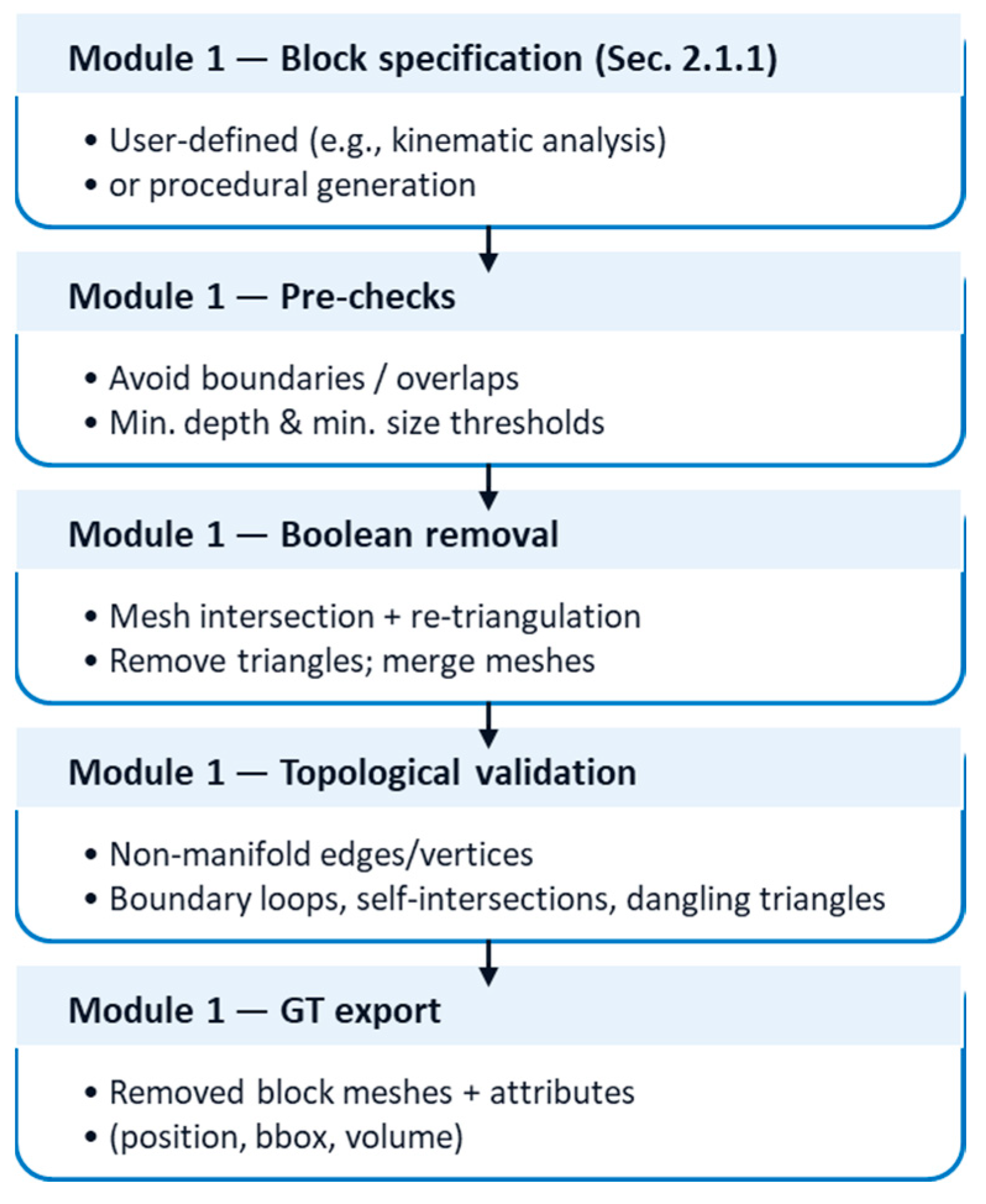
The full workflow for the rock block detachments is reported briefly in Figure 2 and more operationally summarized in Algorithm 1. Starting from the undisturbed rock-face mesh, the simulator generates or imports candidate blocks, places them on the rock surface, validates the resulting intersection, updates the mesh, and stores the corresponding ground-truth annotations.

Algorithm 1 provides the algorithmic sequence implemented to generate the noise-free post-failure geometry and the associated ground truth (GT). The following paragraphs describe the main steps of the algorithm in more detail, distinguishing between user-defined and procedurally generated blocks, block placement, mesh intersection, validity checks, and GT export.

Algorithm 1 Generation of noise-free rockfall GT datasets through iterative block-removal simulation. Simulation configuration parameters consist of: safe-zone mask boundary offset, raster grid step, minimum block size, minimum depth, topology checks flags (enabled/disabled), maximum failed attempts, etc.

Input: Reference rock-face mesh M0; block source or block generator (user-defined blocks or procedural generators) G; target number of detachments N; Simulation configuration C; (opt. for procedural generators) block mesh transformation/modifier pipeline T. Output: Post-failure noise-free mesh Mclean; CRS transform CRS_T; list of removed blocks and metadata GT (Ground Truth). 1: Set CRS_T ← Compute CRS transform from original to rock-wall best-fit plane         orientation (XY plane is parallel to best-fit plane) 2: Set M0* ← CRS_T(M0) 3: Compute the safe-zone raster mask S from M0* and the user-defined boundary offset 4: Set failed_attempts ← 0 5: while |GT| < N and failed_attempts ≤ C.max_failed_attempts do 6:         Generate or load a candidate block B from G: 7:         if procedural generation is used then 8:                  sample a base shape (e.g., prismatic, ellipsoidal, trapezoidal, pyramidal) 9:                  sample the generator parameters for T 10:                apply the user-defined modifier pipeline T                      (e.g., scaling, rotation, roughness perturbation, skewing) 11:                Set B ← resulting modified block mesh (GenerateBlock(G, C, T)) 12:         else if real/user-defined blocks are used then 13:                read the block mesh 14:                 (opt.) enforce convexity 15:                 (opt.) subdivide/add noise to vertices/remesh the block 16:                 B ← CRS_T(B): Transform the block in the working CRS 17:                 Set B ← resulting modified block mesh (Sample_and_Modify_Block(G)) 18:         end if 19:         if procedural generation is used then 20:                Sample the candidate B XY detachment position 21:         else if real/user-defined blocks are used then 22:                Read the XY candidate B detachment position 23:         end if 24:         Set B′ ← transform_and_place(B, M) (i.e., transform and position the block on                      the rock face along Z direction) 25:         Set Ai ← Extract the local mesh patch Ai from M around the bounding box of B′ 26:         Set (Hi, Aminus, Binside, Ci) ← Mesh_intersection(Ai, B′)                      Hi = portion of the local rock-face patch Ai removed by the candidate block                      Aminus = retained portion of the local rock-face patch after removing Hi                      Binside = portion of B’ intersecting the rock face inside the rock-wall                      Ci = block-derived closing surface used to seal the detachment niche 27:         if the removed area Hi is split into disconnected components then 28:                generate a distinct removed block set (more than one B′) 29:         end if 30:         Reject B′ if any enabled validity condition (C.block_checks) is not satisfied:                      B′ intersects the boundary or falls outside the safe zone S                      B′ overlaps a previously accepted detachment                      Binside is empty or geometrically invalid                      the removed area Hi is smaller than the minimum size                      the detachment depth is below the minimum threshold                      the operation creates non-manifold edges, self-intersections, open unwanted                       boundaries, or isolated triangles 31:         if B′ is rejected then 32:                failed_attempts ← failed_attempts + 1 continue 33:         else if B′ is accepted then 34:                failed_attempts ← 0 35:                Store the accepted detachment in GT:                          - removed block mesh                          - detachment niche                          - block ID                          - bounding box                          - volume                          - raster mask/annotation support 36:         end if 37: end while 38: for each accepted block i in GT: 39:         update the mesh by removing Hi from Mi−1 and inserting the closing surface Ci               according to Equation (1) 40: Set Mclean ← resulting mesh MN 41: return Mclean, CRS_T and GT

The first steps consist of initializing the working geometry used throughout the block-removal procedure. The original rock-face mesh is first transformed into a local rock-wall reference frame, in which the $\mathrm{X}\mathrm{Y}$ plane is parallel to the best-fit plane of the rock-wall surface (Algorithm 1, line 2). This working frame simplifies the subsequent raster-based masking operations, the definition of candidate block positions, and the interpretation of block penetration approximately along the local depth direction. A safe-zone mask is then computed from the transformed reference mesh and from the user-defined boundary offset, in order to prevent candidate detachments from intersecting open mesh borders or poorly constrained edge regions (Algorithm 1, line 3). The algorithm then enters an iterative generation loop: candidate blocks are generated or loaded one at a time and are accepted only if all enabled geometric and topological validity checks are satisfied. If a candidate block is rejected, the failed-attempt counter is increased; the procedure stops when either the target number of accepted detachments is reached, or the maximum number of failed attempts is exceeded. This stopping criterion avoids endless iterations in configurations where the remaining valid surface area is too limited or where the selected block-generation parameters are incompatible with the geometric constraints imposed by the rock-face mesh.

As anticipated, the simulator removes a set of blocks from the rock face by reshaping its surface, thus representing material detachment events. These blocks can be explicitly specified by the user, for instance, based on the results of a kinematic analysis of potentially unstable blocks. This option enables the generation of physically informed data that more closely approximates natural detachment processes, ensuring that the location, size, and shape of the removed blocks are consistent with the geotechnical characteristics of the investigated rock face.

In such cases, the simulator may still apply modifications to the geometry or topology of the block model to generate geometrically more complex shapes than those typically obtained from three-dimensional kinematic analyses (blocks identified through stability analyses are often derived from simplified representations of the rock face and tend to exhibit overly regular geometries). In these cases, the simulator can modify the geometry of the block to be removed by enforcing convexity constraints (this is commonly observed in typical rockfall block shapes) and introducing surface irregularities (Algorithm 1, lines 12–17). This is achieved by increasing the number of triangles composing the block mesh, thereby enhancing its ability to represent fine-scale geometric detail, and by perturbing the positions of the mesh vertices.

Alternatively, or in addition to user-defined blocks, the blocks to be removed can be generated procedurally by the simulator (Algorithm 1, lines 7–11). The computational framework is designed to be scalable, allowing the introduction of new block characteristics or generation strategies. At the current stage of development, the simulator includes several procedural generators supporting different block shapes, including cubic/prismatic, spherical/ellipsoidal, trapezoidal, and pyramidal geometries. Within a single simulation, blocks of different shapes may coexist, and the user can specify the probability of occurrence for each shape category. Once a base shape is generated, the simulator applies a sequence of modifiers aimed at randomising the geometric characteristics of each block. For example, one modifier alters block dimensions by applying isotropic or anisotropic scaling factors to the mesh vertices; another modifier rotates the block to simulate its spatial orientation relative to the rock surface; a further modifier introduces surface roughness by randomly displacing mesh vertices along the local surface normal direction; finally, a skew deformation can be applied to the entire mesh using a 3D affine transformation. Modifiers are applied sequentially in a user-defined order, and the same modifier may be applied multiple times within the transformation pipeline, enabling the definition of highly complex and diverse geometric transformations.

Each modifier depends on a set of parameters; for instance, the scaling modifier depends on three independent scale factors along the spatial axes, while the rotation modifier depends on three rotation angles. Each parameter can be associated with a random generator, allowing different transformation values to be used for each generated block. The simulator currently supports multiple types of random generators to accommodate different probability distributions. While uniform or Gaussian distributions are sufficient in many cases, the user may also define custom random generators by explicitly specifying a probability density function.

The spatial placement of procedurally generated blocks (Algorithm 1, lines 19–20) can also be determined randomly. The simplest approach consists of uniform random placement over the entire extent of the rock face.

Once a procedural block has been generated and a detachment zone on the rock face has been selected, the simulator overlaps the block and rock-face meshes and translates the block along the direction orthogonal to the rock surface at that location (Algorithm 1, line 24). This translation continues until the optimal detachment position (i.e., defined as the configuration that maximizes the resulting detachment niche area and volume) is identified. These criteria ensure that the block detached in this way matches as closely as possible the original shape and size of the procedurally generated block.

Once the position of the block relative to the rock face has been determined, the system performs a series of validation checks (Algorithm 1, lines 25–30) to detect potential conflicts with previously removed elements and to ensure that the block removal does not introduce artefacts or topological inconsistencies in the resulting mesh. Specifically, the simulator might verify that: (i) the block does not overlap a boundary edge of the rock-face mesh, thereby avoiding partial intersections with open mesh borders; (ii) the block does not intersect areas previously affected by the removal of other blocks, preventing overlapping detachment niches or duplicated ground-truth annotations; (iii) the block penetrates the rock surface to a sufficient depth, avoiding unrealistically shallow detachments; (iv) the detached block does not fall below a user-defined minimum size threshold, preventing the generation of too small fragments that could bias change detection evaluation; (v) the removal operation does not introduce topological defects in the resulting mesh, including non-manifold edges or vertices, boundary loops (unintended holes), self-intersections, or dangling (isolated) triangles.

These validation steps are performed prior to finalising the detachment event. If any of the above user-selected conditions are violated, the block placement is rejected or adjusted, thereby preserving geometric consistency, numerical stability, and topological validity of the simulated post-failure model.

In compact form, for each accepted detachment $i$, the candidate block is first generated or loaded (Algorithm 1, lines 7–23) and then transformed into the rock-face Coordinate Reference System (CRS). A local mesh patch $A_i\subset M_{i-1}$, where $M_{i-1}$ is the rock-face mesh before the $\mathrm{i}$-th accepted removal, is isolated around the candidate block, and Boolean mesh operations are used to compute both the portion of the rock face removed by the block H_i and the block surface required to close the detachment niche (Algorithm 1, lines 25–26). In other words, this operation (Algorithm 1, lines 25–26) identifies the rock-face portion to be removed, H_i, and the block-derived surface C_i used to close the resulting detachment niche. The retained part of the local rock-face patch, A_minus, and the internal portion of the block, B_inside, are intermediate mesh-processing products used to construct the final replacement geometry. The updated post-failure mesh $M_i$ at the i-th step (i.e., detached block i) can be written schematically as

$$M_i=(M_{i-1}\setminus H_i)\cup C_i$$

(1)

where $C_i$ denotes the closing surface derived from the accepted block/rock-face intersection (Algorithm 1, lines 26 and 39). This notation is intended only as a compact representation of the implemented mesh-processing workflow; the actual implementation performs local mesh isolation, Boolean difference, triangle removal, mesh merging, duplicate vertices merging, and topological validity checks.

In some cases, particularly where the rock surface is highly irregular or characterized by pronounced discontinuities, the intersection between the block and the rock face may result in multiple distinct detachment niches. In such situations, the simulator identifies each niche separately and, for GT annotation purposes, generates a distinct removed block for each of them (Algorithm 1, lines 27–29) rather than treating the event as a single detachment.

At the end of this first stage (Algorithm 1, line 41), the simulator provides two 3D digital models representing the pre- and post-failure morphology of the rock face, unaffected by measurement noise, together with a complete and exact list of all detached blocks and their characteristics (e.g., shape, dimensions, and spatial location).

2.1.2. Photogrammetric Survey Simulation

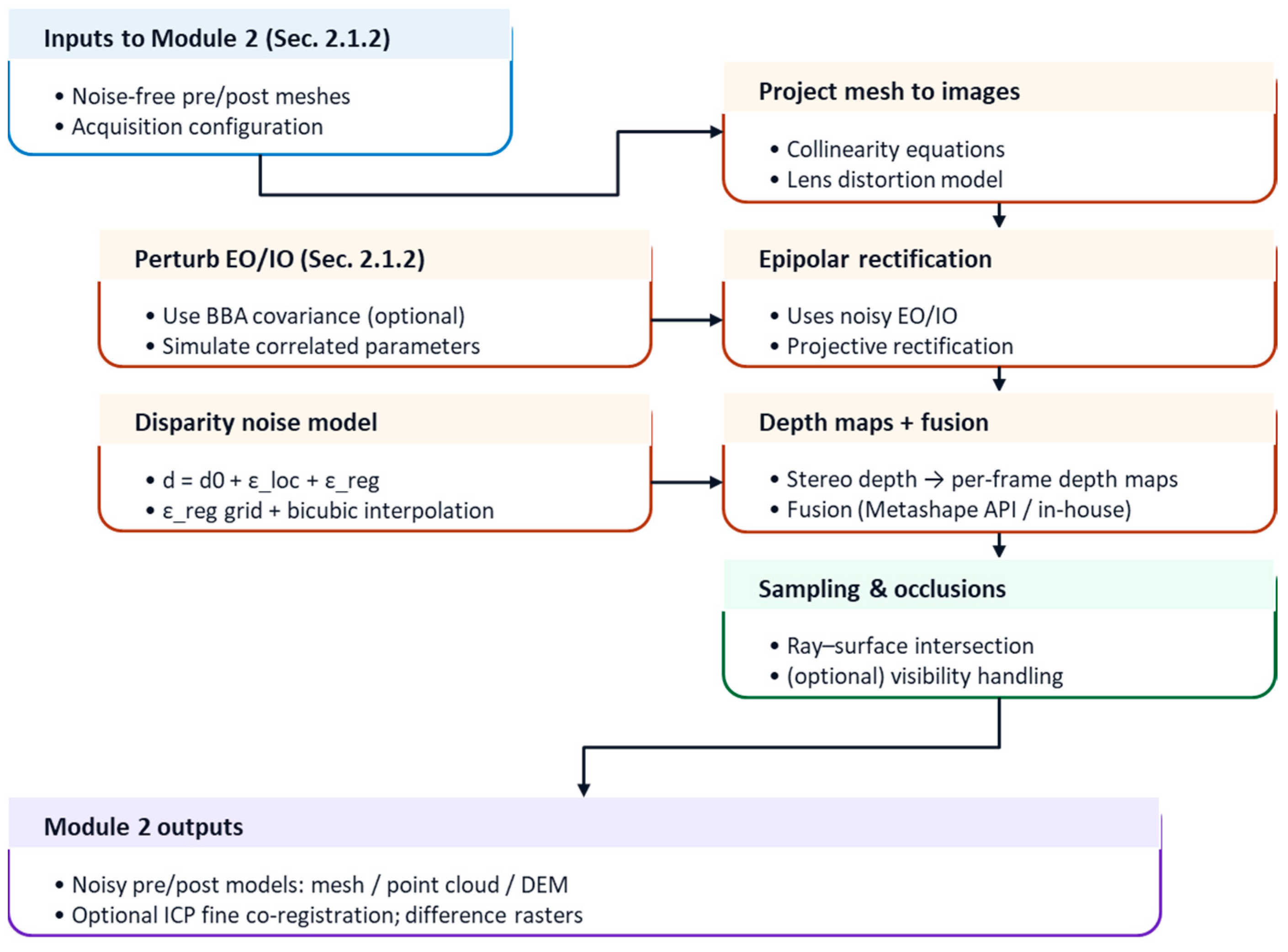
Once the two models (pre- and post-event) representing the GT (i.e., free from any measurement noise) are available, they must be regenerated by explicitly accounting for the selected photogrammetric survey configuration and its associated stochastic characteristics. Starting from a fully error-free configuration, the simulator randomly perturbs all parameters that govern the reconstruction of the 3D model. To this end, the simulator reproduces the full photogrammetric processing pipeline commonly adopted in Multi-View Stereo (MVS) applications, with the objective of generating a noisy 3D reconstruction (Figure 3).

While it would be substantially simpler to render two textured images and perform the matching stage using existing routines implemented in standard photogrammetric software (e.g., Agisoft Metashape [33]), this approach would introduce two major drawbacks. First, generating a realistic rock-surface texture (e.g., procedurally) would add an additional layer of complexity and could increase the gap between the simulation and realistic conditions. Conversely, using a real texture (e.g., extracted from the rock wall employed to generate the 3D models) would still require procedural texture synthesis in areas affected by simulated detachments, thus reintroducing the same issue. Second, such a strategy would prevent generating multiple independent simulations for the same rock face, undermining one of the simulator’s main objectives, namely producing a large number of test or training instances starting from the same underlying morphology.

Physically based radiative-transfer and sensor-simulation frameworks (e.g., DART [34]) could explicitly model spectral, atmospheric, and illumination acquisition effects in complex scenes. However, adopting that level of radiometric simulation (with RGB imaging, an additional level of complexity would be introduced) would require a substantially broader set of assumptions and calibration data that are not available in common applications. More importantly, it would not directly address the main target of this work, namely the generation of DEM-level photogrammetric noise fields compatible with real repeated measurements. Consequently, the proposed framework deliberately bypasses explicit image rendering and models the relevant uncertainty directly at the camera-geometry, disparity, depth-map, and reconstructed-surface levels and does not explicitly simulate radiometric or image-quality disturbances such as cast shadows, illumination changes, motion blur, or vegetation-related occlusions. Their aggregate effect may be partly reflected in the empirical real-noise baseline used for calibration (see Section 2.2 and Section 3.1), but they are not controlled independent variables of the simulation.

Algorithm 2 provides the algorithmic sequence implemented to generate the noisy pre- and post-failure geometry. The following paragraphs describe the main steps of the algorithm in more detail.

Algorithm 2 Simulation of photogrammetric survey uncertainty and generation of noisy reconstructed datasets from noise-free ground-truth models. Processing configuration parameters include image safe-border size, depth-map downscale factor, visibility/occlusion filtering options, use of external depth-map fusion, optional ICP-based registration, output resolution, export format, etc.

Input: Noise-free meshes (pre-failure or post-failure surface) Mpre_clean and Mpost_clean; CRS transform CRS_T; calibrated photogrammetric project/image block P; uncertainty model for EO/IO parameters U0 (e.g., εθ ∼ N$(\mu , {\mathsf{\Sigma }}_{\mathrm{BBA}})$ when the BBA covariance matrix is used); image matching uncertainty model parameters $({\sigma }_{\mathrm{loc}}^2, {\sigma }_{\mathrm{reg}}^2, L_{reg})$; processing configuration parameters 1 C. Output: Pre- and post-failure noisy meshes Mpre_noisy and Mpost_noisy; (opt.) optional depth maps list D for each epoch; (opt.) optional raster products, point clouds and masks R. 1: Import the photogrammetric image block P 2: Set P* ← CRS_T(P) 3: for each epoch mesh Mclean in (Mpre_clean, Mpost_clean) do 4:         Initialize the depth-map list D ← empty list 5:         Generate the noisy camera block P′epoch by perturbing the EO/IO of P*:                      θ′ ← θ + εθ              where θ contains the selected EO/IO parameters and εθ is sampled from U0 6:         for each stereo pair k (Ii, Ij) in P′epoch do 7:                  Compute the epipolar rectification for the stereo pair using the noisy camera                      parameters in P′ 8:                  Generate regularized matching-noise on a coarse rectified image grid ${\mathbf{g}}_{ij}:$                                    ${\epsilon }_{\mathrm{reg}}\left({\mathbf{g}}_{ij}\right)\sim \mathcal{N}\left(0,{\sigma }_{\mathrm{reg}}^2\right)$ 9:                  Project the vertices and triangles of Mclean onto the original image planes                      using the noise-free camera parameters and the selected lens-distortion                      model by collinearity equations. 10:                Transform the projected image coordinates into the rectified image planes 11:                Apply image-domain validity checks:                             - projected points inside the image frame                             - projected points inside the user-defined safe image border                             - finite and valid depth values                             - valid triangle projection 12:                Apply visibility and occlusion checks, if enabled in C:                             - remove points or triangles not visible from the considered camera                             - remove triangles producing inconsistent projection 13:                Compute the ideal rectified disparity field $d_0\left(\mathbf{p}\right)$ for the valid projected                      samples $\mathbf{p}$ = (x, y) 14:                Sample the local pixel-wise matching-noise component:                                    ${\epsilon }_{\mathrm{loc}}\left(\mathbf{p}\right)\sim \mathcal{N}(0,{\sigma }_{\mathrm{loc}}^2)$ 15:                Interpolate the regularized noise from the grid nodes to each valid pixel:                                    ${\epsilon }_{\mathrm{reg}}\left(\mathbf{p}\right)\hspace{0.25em} =\hspace{0.25em} {\mathcal{I}}_{\mathrm{bicubic}}\left(\left\{{\epsilon }_{\mathrm{reg}}\right({\mathbf{g}}_{ij}\left)\right\}\right)\left(\mathbf{p}\right)$ 16:                Compute the total matching-noise contribution:                                    ${\epsilon }_{\mathrm{match}}\left(\mathbf{p}\right)={\epsilon }_{\mathrm{loc}}\left(\mathbf{p}\right)+{\epsilon }_{\mathrm{reg}}\left(\mathbf{p}\right)$ 17:                Add matching noise to the ideal disparity field:                                    $d\left(\mathbf{p}\right)\hspace{0.25em} =\hspace{0.25em} d_0\left(\mathbf{p}\right)\hspace{0.25em} +\hspace{0.25em} {\epsilon }_{\mathrm{match}}\left(\mathbf{p}\right)$ 18:                Convert the noisy disparity field $d\left(\mathbf{p}\right)$ into 3D coordinates using the                      rectification reprojection matrix:                                    $X^{\prime }(\mathbf{p}$$) \leftarrow \mathit{Reproject}(\mathbf{p}$$, d\left(\mathbf{p}\right)$) 19:                Generate the noisy depth maps Dk_i and Dk_j for the stereo pair 20:       end for 21:       Merge together the depth maps corresponding to the same image:                     Di ← FuseDepthMaps(Dk_i) 22:       Add Di to the depth-map list D 23:       if external depth-map fusion is enabled in C then 24:               Convert the simulated depth maps D into the required software format D*                     (e.g., Metashape-compatible depth maps) 25:               Replace or inject the depth maps D* into the photogrammetric project 26:               Run the selected depth-map fusion/mesh-generation procedure 27:               Set Mnoisy ← fused triangulated mesh 28:       else 29:               Run the internal depth-map fusion/mesh-generation procedure 30:                Set Mnoisy ← internally fused triangulated mesh 31:       end if 32:       Remove invalid mesh elements from Mnoisy:                             - non-finite vertices                             - degenerate triangles                             - isolated or null triangles                             - triangles outside the valid reconstruction mask 33:       (opt.) compute normals and clean duplicate vertices from Mnoisy 34: end for (at this point Mpre_noisy and Mpost_noisy have been computed) 35: if fine co-registration is enabled in C then 36:       align Mpost_noisy to Mpre_noisy using the selected registration method (e.g., ICP) 37: end if 38: Export Mpre_noisy and Mpost_noisy in the requested output formats:                             - triangulated mesh                             - point cloud                             - raster DEM 39: return Mpre_noisy, Mpost_noisy and optional outputs D and R

The first steps of Algorithm 2 initialize the photogrammetric survey simulation in the same rock-wall reference frame used for block removal. The calibrated image block is transformed consistently with the input mesh, and a perturbed camera block is generated by sampling the selected EO/IO uncertainty model. The procedure is then repeated independently for each simulated epoch mesh, so that the pre- and post-failure surfaces are reconstructed as separate noisy acquisitions. For each selected stereo pair, the simulator computes the rectified geometry, projects the noise-free mesh into image space, perturbs the ideal disparity field through the matching-noise model, and reconstructs a noisy depth surface. The resulting depth maps are finally fused into a triangulated mesh, optionally co-registered and exported in the required formats.

First, the user needs to specify how the simulated image block $P$ is configured, including the number of images, the image-block geometry, camera calibration, and processing options (Algorithm 2, input and lines 1–2). For each simulated epoch, the simulator generates a noisy camera block by perturbing the selected EO and IO parameters according to the adopted uncertainty model (Algorithm 2, line 5), θ′ = θ + εθ, where θ contains the EO and/or IO parameters, and εθ is sampled either from independent user-defined distributions or from a multivariate distribution derived from the BBA covariance matrix. The photogrammetric simulator then emulates a MVS dense-matching process (Algorithm 2, lines 6–34). The images are considered together with their orientation parameters, both in the noise-free and noise-perturbed configurations. Using the error-free parameters, the vertices of the rock-face mesh are projected onto each image plane through collinearity equations (Algorithm 2, line 9). This step defines the ideal geometric image projection of the mesh, not a rendered textured image. Although lens distortion effects are accounted for (here assumed to be perfectly represented by the selected distortion model, e.g., the Brown-Conrady model [35]), this ideal image would not, by definition, be affected by estimation errors in the orientation parameters.

To simulate dense-matching in an MVS procedure, each selected stereo-pair (two images) undergoes an epipolar rectification procedure. Specifically, a projective rectification approach is adopted, in which a homography is computed between each image plane and an optimal plane that is parallel to the stereo baseline and as little inclined as possible with respect to both image frames (Algorithm 2, lines 8 and 10). Rectification presupposes knowledge of internal and external orientation parameters, which, in the real world, may be derived from estimation procedures, pre-calibration, or, in the case of direct georeferencing, auxiliary sensors (e.g., IMU + GNSS (Inertial Measurement Unit + Global Navigation Satellite System)). Consequently, this stage is inevitably affected by measurement/estimation noise, interpreted here as uncertainty in the parameters. The epipolar rectification procedure itself must incorporate the effects of parameter noise. The epipolar rectification is computed consequently from the noisy camera block, while the mesh projection is obtained from the noise-free geometry and subsequently transformed into the rectified image planes (Algorithm 2, lines 8–10). To this aim, as in the rockfall simulation stage, the user may select different random generators to model measurement noise. In this context, however, the most appropriate choice is to adopt a generator that explicitly accounts for the multivariate distribution describing the uncertainty of these parameters (e.g., the parameter covariance matrix typically provided by photogrammetric software at the end of Bundle Block Adjustment (BBA)). Indeed, internal and external orientation parameters are strongly correlated, both within each parameter set and across sets. Ignoring their covariance structure may result in unrealistic parameter combinations and, consequently, non-physical error patterns in the reconstructed geometry.

The simulator explicitly models the image-matching process between the two epipolar-rectified images. In this context, it becomes important to stochastically model the error characteristics that typically arise during image matching. Most modern commercial software packages (e.g., Agisoft Metashape [33], SURE [36], MicMac [37], etc.), regardless of the specific implementation, adopt global or (more often) semi-global matching strategies to increase robustness and spatial regularity in correspondence estimation, to improve reconstructions in areas with repetitive patterns or low-contrast texture, and to reduce the high-frequency pixel-to-pixel noise commonly produced by purely local matching methods.

The proposed workflow deliberately does not rely on explicit surface texture information. In Algorithm 2, this corresponds to perturbing the ideal disparity field directly, rather than simulating the image-matching cost function on rendered images (Algorithm 2, lines 13–18). The simulator models matching uncertainty directly on the disparity field by decomposing it into two components: (i) a local (pixel-wise) component, represented as a random variable, and (ii) a larger-scale component representing the spatially smooth regularization effect induced by global or semi-global constraints. A process-level simulation of the error sources of a specific matching algorithm would require modelling the image texture, radiometric conditions, matching cost function, aggregation or regularization parameters, confidence filtering, and implementation-specific post-processing. This would introduce an additional texture- and algorithm-dependent layer of complexity, which is deliberately outside the scope of the present texture-independent simulator. In other words, the proposed disparity-noise model is not intended to reproduce the internal cost aggregation or optimisation of a specific matching algorithm such as SGM. Instead, it provides a phenomenological representation of the two dominant effects relevant at the DEM-difference level: local disparity uncertainty and spatially correlated regularisation effects. Its adequacy is therefore assessed empirically by comparing the resulting noise fields with real DEM-difference rasters through variogram, spectral, and roughness descriptors (see Section 2.2 and Section 3.1). To model the regularization of the disparity field, a regular grid with user-specified spacing over the image domain is defined. A random noise value is generated at each grid node. The probability distributions for both components can be specified by the user; however, preliminary tests indicated that a Gaussian distribution provides the most satisfactory results. For pixels not coincident with grid nodes, the regularization-related contribution is obtained by bicubic interpolation. In other words, the disparity $d\left(\mathbf{p}\right)$ at pixel $\mathbf{p}=(x,y)$ is defined as

$$d\left(\mathbf{p}\right)\hspace{0.25em}=\hspace{0.25em}{d}_0\left(\mathbf{p}\right)\hspace{0.25em}+\hspace{0.25em}{\epsilon }_{\mathrm{match}}\left(\mathbf{p}\right)$$

(2)

where $d_0\left(\mathbf{p}\right)$ is the “ideal” disparity between corresponding points on the simulated epipolar rectified image pair, thus affected by interior (IO) and exterior orientation (EO) noise, but immune to matching noise ${\epsilon }_{\mathrm{match}}\left(\mathbf{p}\right)$ which is computed as

$${\epsilon }_{\mathrm{match}}\left(\mathbf{p}\right)={\epsilon }_{\mathrm{loc}}\left(\mathbf{p}\right)+{\epsilon }_{\mathrm{reg}}\left(\mathbf{p}\right)$$

(3)

where the local component is generated randomly (e.g., using a normal distribution with zero mean and ${\sigma }_{\mathrm{loc}}^2$ variance: ${\epsilon }_{\mathrm{loc}}\left(\mathbf{p}\right)\sim \mathcal{N}(0,{\sigma }_{\mathrm{loc}}^2)$:

$${\epsilon }_{\mathrm{reg}}\left({\mathbf{g}}_{ij}\right)\sim \mathcal{N}\left(0,{\sigma }_{\mathrm{reg}}^2\right) {\epsilon }_{\mathrm{reg}}\left(\mathbf{p}\right)\hspace{0.25em}=\hspace{0.25em}{\mathcal{I}}_{\mathrm{bicubic}}\left(\left\{{\epsilon }_{\mathrm{reg}}\right({\mathbf{g}}_{ij}\left)\right\}\right)\left(\mathbf{p}\right)$$

(4)

These equations correspond to the operations summarized in Algorithm 2, lines 13–17.

Once the disparity field has been computed, the corresponding depth field for the stereo pair can be readily derived, and from it, the depth map associated with each individual image can be obtained. This corresponds to the reprojection and depth-map generation steps in Algorithm 2, lines 18–22. At this stage, the simulator may either rely on the depth-map fusion algorithms implemented in commercial software packages (Algorithm 2, lines 23–27—currently, an interface has been developed via Python 3.9+ APIs to enable interoperability with Agisoft Metashape) or use proprietary algorithms to perform the same operation (Algorithm 2, lines 28–30). In the configurations used in this work, this step is applied to the selected stereo pair; the same structure can be extended to multiple selected stereo pairs when multi-image depth-map fusion is enabled.

At the end of the procedure, the final output is a triangulated mesh analogous to the initial one but perturbed by noise introduced at the various stages of the photogrammetric pipeline. This mesh may undergo further processing (e.g., a common step in change detection workflows is the fine co-registration of the mesh to a reference model, for instance via Iterative Closest Points (ICP)-based methods [38]) and can be exported or converted into different representations and formats (e.g., point clouds, raster products, etc.). The final cleaning, optional fine co-registration, and export steps are summarized in Algorithm 2, lines 32–39.

2.2. Noise Calibration and Validation

As previously mentioned, a fundamental requirement for the simulator is to minimise the so-called sim-to-reality gap. In practical terms, this means that the simulator must generate data that is statistically and physically plausible, and comparable to those that would be obtained in a real monitoring scenario of a rock face undergoing natural evolution and potential rockfall events. While the possibility of using a deterministic approach based on stability analysis for block removal (see Section 2.1.1) shifts the issue of realism toward the validity of the stability model itself (note that this aspect lies outside the scope of the current simulator), the correct validation and, if necessary, calibration of the stochastic measurement noise model becomes critical.

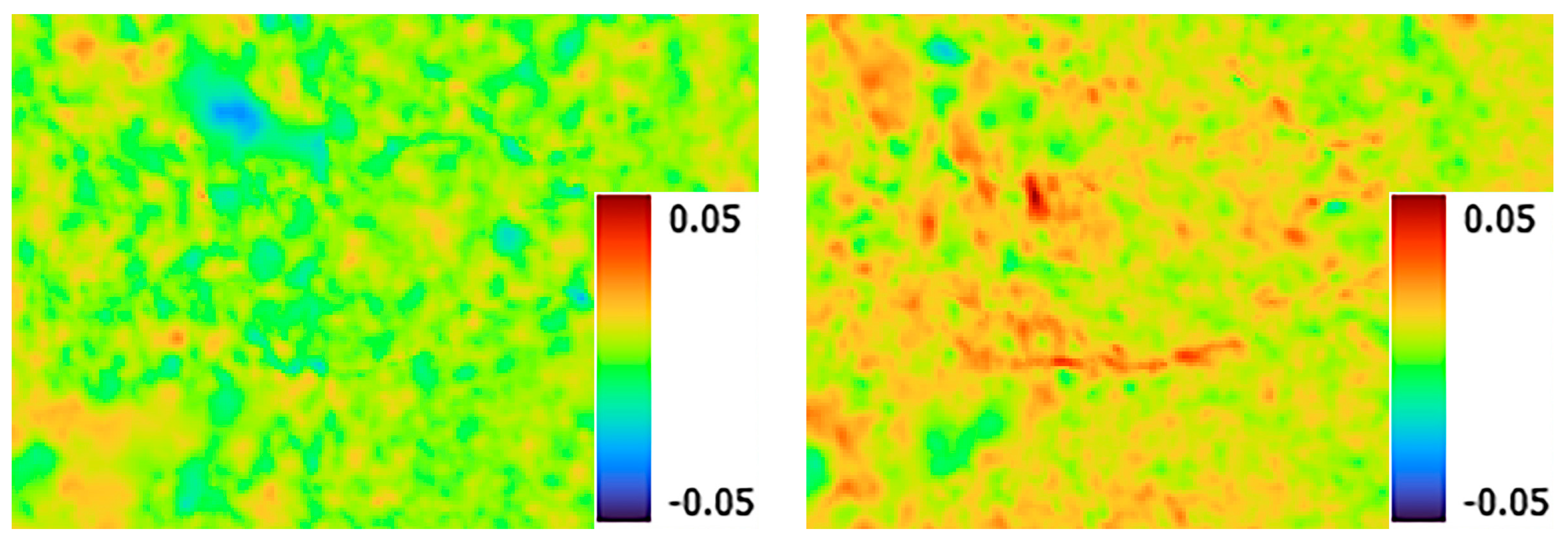
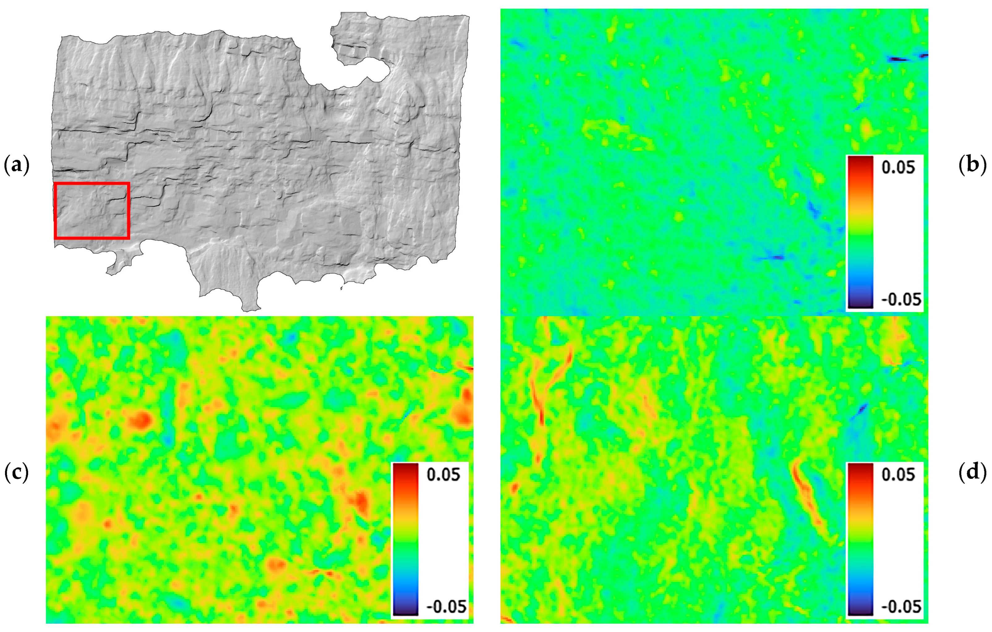
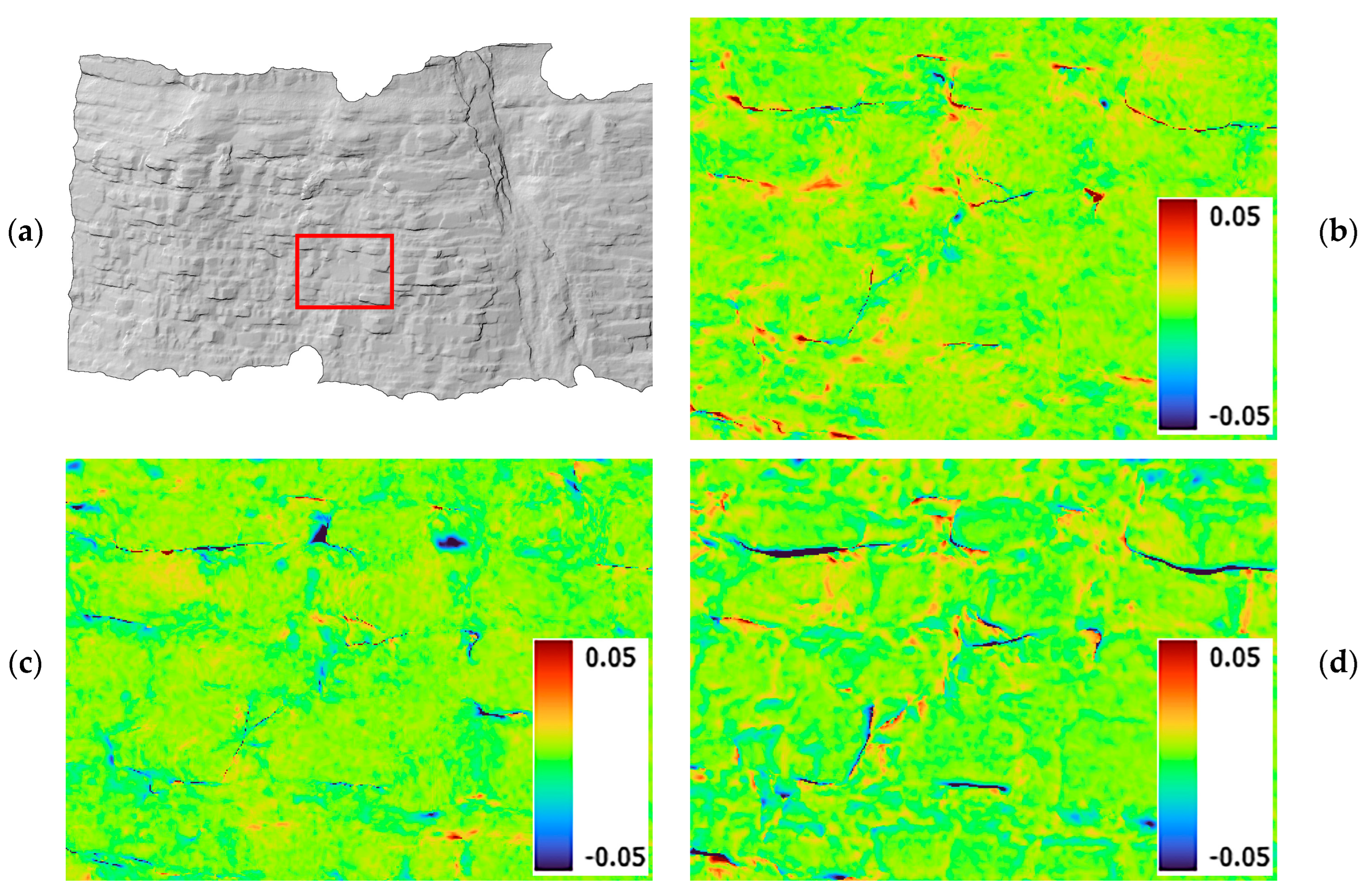
In other words, it is important to assess whether two datasets representing differences between surfaces (one derived from real measurements and the other generated through simulation) can be regarded as statistically compatible realisations of the same underlying spatial stochastic measurement process. Figure 4 shows a false-colour representation of DEM differences (the colour bar is in the range ± 0.05 m) in an undisturbed (i.e., without rockfalls or actual displacements, for simplicity in a flat/planar rock area) in two real case acquisitions.

In the following, the term measurement noise is used in an operational sense to denote the residual DEM-difference field observed between two nominally unchanged surfaces. This effective noise field is not limited to sensor noise alone, but also includes photogrammetric reconstruction uncertainty, dense-matching uncertainty, residual co-registration errors, occlusion- and completeness-related artefacts, rasterization effects, and other modelling approximations that affect real pre-/post-event comparisons. When needed, the terms EO/IO parameter uncertainty, matching uncertainty, and registration error are used to refer to specific components of this broader effective measurement-noise field.

Because measurement noise is random by nature, comparing two raster fields pixel by pixel is not very informative, whether the comparison is between two real difference maps or between a real and a simulated one. Even a very good simulation, capable of reproducing the same statistical behaviour as the real noise, would not generate the same value at the same pixel location. For this reason, the comparison should focus on the overall statistical properties of the fields, rather than on the exact values of individual pixels.

As previously pointed out, to focus only on the stochastic features of real and simulated noise, the following analysis considers surface differences computed between models that are nominally unaffected by rockfall events. In the case of real data, models were selected from surveys acquired over sufficiently short time intervals, where possible, to ensure that no significant morphological changes could have occurred. This assumption was also verified by expert visual inspection. In the case of simulated data, the analysis was conducted by generating pre- and post-event models without removing any blocks.

In the absence of measurement noise, the two models in both cases would be identical, and their differences would ideally be zero everywhere. The observed differences, therefore, represent spatially distributed random fluctuations resulting from measurement uncertainty and modelling approximations. These fluctuations characterise the stochastic structure of the measurement noise.

To improve computational efficiency and enable a consistent statistical characterization of noise patterns, in the following analysis, surface differences are represented, as in Figure 4, as a two-dimensional raster, i.e., a scalar 2D spatial field. The two 3D models are then projected and rasterized onto a best-fit rock-face plane, and differences are then evaluated by raster difference. This choice reduces computational costs and facilitates the use of standard spatial-statistics tools (e.g., correlation and spectral analyses) working on a regular grid.

It is worth noting that this representation also makes the contribution of residual misregistration between the pre- and post-event models (e.g., residual rigid-body errors after ICP) more evident. In the adopted planar parameterization, portions of the rock face whose local surface normals are strongly inclined with respect to the best-fit plane are mapped in foreshortened view. As a consequence, even small residual alignment errors can be amplified in the rasterized difference field, producing locally large apparent changes despite the absence of true morphological evolution. Such residual misregistration should be treated as an integral component of the effective measurement process, together with sensor noise and reconstruction uncertainty, because it systematically affects real pre/post comparisons and is therefore expected to be reproduced by a realistic simulator.

The methodological framework adopted in this work evaluates the compatibility of the two noise raster fields by jointly analysing: (i) their marginal distributions, (ii) their spatial correlation structure (variogram), (iii) their spectral characteristics, and (iv) their scale-dependent roughness. These descriptors capture complementary statistical properties of spatial random fields and provide a robust basis for assessing stochastic similarity between simulated and real measurement noise. The marginal distribution captures the first-order properties of the fluctuations, the variogram describes second-order spatial dependence, the power spectrum provides a global multiscale representation of spatial energy, and roughness analysis characterizes the hierarchical structure of fluctuations across scales.

These descriptors were selected according to four criteria: (i) complementarity, (ii) interpretability in terms of photogrammetric error sources (for instance marginal distribution metrics are strongly influenced by the magnitude of the noise parameters, variogram and power spectrum descriptors allow fine-tuning the regularization vs. local noise deriving from the EO/IO and matching uncertainties, etc.), (iii) computability on regular DEM-difference rasters, and (iv) diagnostic usefulness for simulator calibration.

Consistent agreement across these complementary descriptors provides strong evidence that the measured and simulated fields can be regarded as statistically compatible realisations of the same underlying spatial stochastic process, whereas discrepancies in individual metrics offer diagnostic insight into specific aspects of the simulation model that may require further refinement. In the following, each descriptor or group of descriptors will be briefly introduced.

2.2.1. Marginal Distribution of Noise

The input data consists of a scalar field discretised on a regular grid. We computed marginal (pointwise) distribution statistics from each raster by treating all valid grid values as an independent sample $\left\{{\mathrm{z}}_{\mathrm{i}}{\}}_{\mathrm{i}=1}^{\mathrm{N}}\right.$ after discarding missing pixels encoded as NaN.

The first-order moment is the sample mean:

$$\overline{z}={\displaystyle \frac{1}{N}}{\displaystyle \sum _{i=1}^N}{z}_i$$

(5)

which provides an estimate of the average bias of the elevation differences. Dispersion is quantified using the (unbiased) sample variance and its square root (sample standard deviation):

$$s^2={\displaystyle \frac{1}{N-1}}{\displaystyle \sum _{i=1}^N}{(z_i-\overline{z})}^2, s=\sqrt{s^2}$$

(6)

To characterise departures from Gaussianity beyond second order, skewness (Equation (7)) and excess kurtosis (Equation (8)) are also computed:

$$\mathrm{s}\mathrm{k}\mathrm{e}\mathrm{w}\mathrm{n}\mathrm{e}\mathrm{s}\mathrm{s}={\displaystyle \frac{{\displaystyle {\sum }_{i=1}^N}{(z_i-\overline{z})}^3}{N·s^3}}$$

(7)

$$\mathrm{e}\mathrm{x}.\mathrm{k}\mathrm{u}\mathrm{r}\mathrm{t}\mathrm{o}\mathrm{s}\mathrm{i}\mathrm{s}={\displaystyle \frac{{\displaystyle {\sum }_{i=1}^N}{(z_i-\overline{z})}^4}{N·s^4}}-3$$

(8)

2.2.2. Empirical Variogram and Fitted Summary Parameters

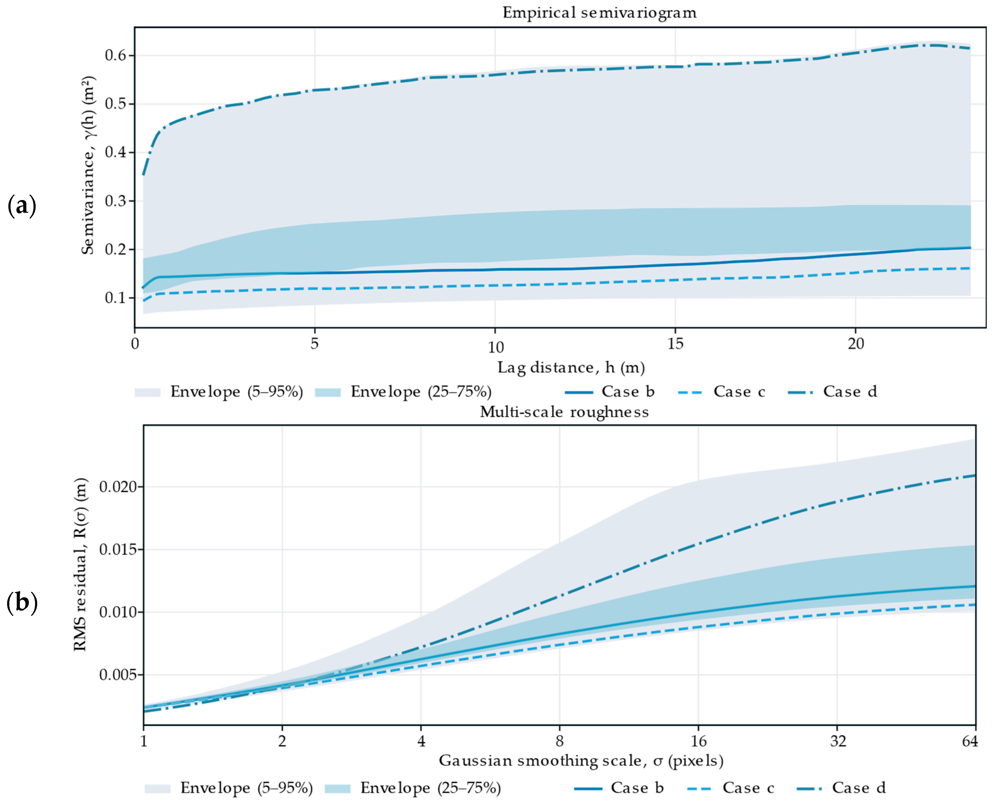
To characterise the spatial correlation structure of the noise field, the isotropic empirical semivariogram for each raster has been computed. For a spatial random field $Z\left(\mathbf{x}\right)$ (where $\mathbf{x}=(x,y)$ represents the location of a raster point, the semivariogram is defined as

$$\gamma (h)={\displaystyle \frac{1}{2}}\hspace{0.17em}\mathbb{E}[(Z(\mathbf{x})-Z(\mathbf{x}+\mathbf{h}){)}^2],$$

(9)

where $h=\parallel \mathbf{h}\parallel$ is the separation distance (lag), and $\mathbb{E}$ is the average operator. In this context, $\gamma \left(h\right)$ measures how dissimilar the field becomes as the distance between samples increases: small values at short distances indicate strong local similarity (spatial correlation), while a plateau at large lags indicates loss of correlation at long distances.

To describe the stochastic characteristics of the noise field, in addition to sampling the full empirical curve $\gamma \left(h\right)$, some scalar descriptors commonly used in geostatistics are considered as well: (i) the nugget, which represents the part of the variability that already appears at very short distances (i.e., the variability that may be due to background noise or highly local fluctuations) and is determined by the height of the first discontinuity of the variogram at the origin; (ii) the sill, which represents the maximum (generally stable) level reached by the variogram at large values of h (i.e., comparing points that are far apart), provides a concise indicator of the level of variability where spatial correlation should have disappeared; (iii) the range, which is the distance h where the semivariogram approaches the sill (i.e., where the spatial correlation can be considered negligible). The range, here interpreted as the practical/effective range, is computed as the distance at which the semivariogram reaches 95% of the sill value, following a common convention in geostatistical applications [39,40].

2.2.3. Two-Dimensional Power Spectrum and Radial Spectral Descriptors

Another element for evaluating the stochastic behaviour of the noise field is represented by the analysis of the values considered in the frequency domain. In particular, the 2D power spectrum, which describes how the variance (energy) of the analysed values is distributed with respect to the spatial frequencies, is considered in the analysis. Smooth and wide-range changes (low spatial frequencies) can highlight if noise connected to global parameters (e.g., EO/IO parameters, regularization of the image matching simulation (Equations (2) and (3)), etc.) is captured adequately by the simulation, while energy at higher frequencies describes the behaviour of the simulation for more localized noise effects (e.g., the pixelwise matching precision in Equation (3)).

Starting from the raster values $Z\left(\mathbf{x}\right)$, the 2D Fast Fourier Transform (FFT) is first computed: this yields the complex Fourier coefficients $F(u,v)$, where $u$ and $v$ are the spatial-frequency coordinates associated with the x- and y-directions, respectively. The 2D power spectrum is calculated as the squared modulus of the complex Fourier coefficients:

$$P\left(u,v\right)={\left|F\left(u,v\right)\right|}^2=F\left(u,v\right)F^{\ast }\left(u,v\right)$$

(10)

To obtain a more synthetic description of the power-frequency field, a radial curve, obtained by averaging the spectral samples with the same radial frequency $f_r=\sqrt{f_x^2+f_y^2}$, is computed.

In addition to the full radial profile $\widehat{P}\left(f_r\right)$, two compact descriptors are computed as well: a spectral slope, computed as the slope of a linear fit of $\mathrm{l}\mathrm{o}\mathrm{g}\widehat{P}\left(f_r\right)$ versus $\log f_r$ considering only the mid-frequency bands (to avoid very low and very high frequencies), and a spectral entropy. Let $\widehat{P}\left(f_{r,k}\right)$ be the radially averaged power associated with the kth radial-frequency bin, the normalized spectral energy in each bin is defined as

$$p_k={\displaystyle \frac{\widehat{P}\left(f_{r,k}\right)}{{\sum }_{k=1}^M\widehat{P}\left(f_{r,k}\right)}}$$

(11)

and the spectral entropy $H$ is then computed as

$$H=-{\sum }_{k=1}^M{p}_k·\mathrm{l}\mathrm{o}\mathrm{g}\left(p_k\right)$$

(12)

In this work, the natural logarithm is used. Changing the logarithm base would only rescale the entropy values and would not affect the relative comparison among real and simulated samples.

Low entropy indicates that spectral power is concentrated in a limited number of frequency bands, whereas high entropy indicates that power is more evenly distributed across frequencies.

2.2.4. Scale-Dependent Roughness

A final set of descriptors for evaluating the stochastic behaviour of the simulation is represented by the multi-scale roughness of each raster. To evaluate how the apparent “roughness” of the field changes with observation scale, a progressive Gaussian smoothing is computed: for a given smoothing scale $\sigma$, where $\sigma$ represents the standard deviation of the Gaussian kernel used via convolution for smoothing the noise field $Z\left(\mathbf{x}\right)$, a smoothed raster $Z_{\sigma }\left(\mathbf{x}\right)$ is computed. The roughness at that scale is then defined as the RMS of the residual between the original field and this smoothed surface:

$$R(\sigma )=\sqrt{{\displaystyle \frac{1}{N}}{\displaystyle \sum _{i=1}^N}{\left(z_i−z_{\sigma ,i}\right)}^2}$$

(13)

By evaluating $R\left(\sigma \right)$ over a set of increasing $\sigma$ values, a roughness “curve” that summarizes the scale dependence of the noise field is computed.

As for the radial power spectrum function, to obtain a compact descriptor, a bilogarithmic power-law linear relationship is fitted. Assuming the scale-dependent roughness can be approximately represented through a linear relation:

$$\log R\left(\sigma \right)\approx a+b\hspace{0.17em}\log \sigma ,$$

(14)

and estimating the intercept $a$ and slope $b$ via least squares allows the roughness to be described with just two synthetic indicators. This power-law relation is not intended as a physical model of the measurement noise, but as an empirical scale-space summary of the roughness curve over the analysed range of smoothing scales. The fitted slope and intercept are therefore used as compact descriptors of the amplitude and scale dependence of the residual field, while the goodness of fit is retained as a diagnostic indicator of the adequacy of this approximation. In particular, the slope $b$ can be interpreted as an indication of how rapidly the roughness changes with scale, while the intercept $a$ indicates the overall amplitude level. The goodness of fit of Equation (14) (i.e., $R^2$ parameter) is considered in all the tests as a diagnostic to verify whether the simple proposed linear law is an adequate approximation over the selected scale interval.

2.2.5. Mahalanobis-Distance Acceptance Model for Noise Validation

To assess whether a simulated noise field is statistically consistent with the variability observed in real measurements, the validation problem was formulated as an acceptance test in feature space. As described in the previous sections, for each raster, a set of complementary descriptors/features (marginal statistics, multi-scale roughness parameters, variogram features, and spectral features) is computed.

During the design and preliminary testing of the validation model, a larger set of candidate descriptors was also considered, including high-dimensional curve-based representations of roughness, variogram and radial power spectrum, as well as fractal dimension, extreme-value and higher-order marginal statistics. However, these descriptors were not retained in the final acceptance model because they were either redundant with the selected features, strongly collinear, highly sensitive to residual outliers, dependent on arbitrary parameter choices, or not reliably identifiable from the available spatial support. For instance, autocorrelation functions provide information closely related to the variogram, while wavelet- and texture-based descriptors introduce a large number of scale-, orientation-, or binning-dependent features that would require a larger number of real samples for stable covariance estimation. Similarly, fractal and extreme-value indicators were found to be sensitive to residual localized artefacts and to the finite size of the raster support. These descriptors were therefore discarded to avoid spurious rejection caused by unstable covariance estimates or by features dominated by numerical and sampling artefacts. These heterogeneous outputs were mapped to a single numerical feature vector $\mathbf{x}\in {\mathbb{R}}^p$.

Using a set of real-noise rasters, obtained as DEM-difference rasters from real data where no rockfall or other surface changes have occurred, an empirical stochastic model of the real-data behaviour was estimated by computing the mean vector and the covariance matrix of the different elements of the feature vector. Because the different features have different physical units and dynamic ranges, a feature-wise standardization using the empirical mean and standard deviation computed from the real samples was performed:

$$z_j={\displaystyle \frac{x_j-{\mu }_j}{{\sigma }_j}},j=1,\dots ,p,$$

(15)

yielding a standardized vector $\mathbf{z}$. This step ensures that the subsequent multivariate distances are not dominated by features with larger numerical scale.

To account for correlations among features (e.g., adjacent scale bins in roughness curves, contiguous frequency bins in spectra, etc.), the covariance structure of the standardized real feature vectors is modelled. In practice, empirical covariance matrices estimated from a limited number of real samples can be ill-conditioned, especially when $p$ is not small or when features are strongly correlated. We therefore applied ridge-regularized whitening, adding a small diagonal term proportional to the average variance before inversion. Denoting by $\mathsf{\Sigma }$ the covariance matrix of standardized real vectors, we consider a regularized matrix ${\mathsf{\Sigma }}_{\lambda }=\mathsf{\Sigma }+\lambda \hspace{0.17em}\overline{v}\hspace{0.17em}I$, where $\overline{v}$ is the mean diagonal element of $\mathsf{\Sigma }$ and $\lambda >0$ controls the amount of regularization. We then compute a whitening transform $W$ (via Cholesky decomposition) such that $W{\mathsf{\Sigma }}_{\lambda }{W}^{\top }\approx I$. In this whitened space, the components are approximately decorrelated and scaled, enabling stable distance evaluation.

Given a candidate feature vector $\mathbf{x}$ of a real or simulated sample, after computing its standardized representation $\mathbf{z}$, the sample’s squared Mahalanobis distance can be computed as

$$D^2(\mathbf{x})={\mathbf{z}}^{\top }{\mathsf{\Sigma }}_{\lambda }^{-1}\mathbf{z}=\parallel W\mathbf{z}{\parallel }^2$$

(16)

This distance quantifies how far the sample lies from the multivariate distribution of real-noise features, accounting for both feature variances and inter-feature correlations. In other words, a sample can be considered “close” to the real baseline model only if it matches not just the marginal ranges of each feature but also their typical joint co-variation.

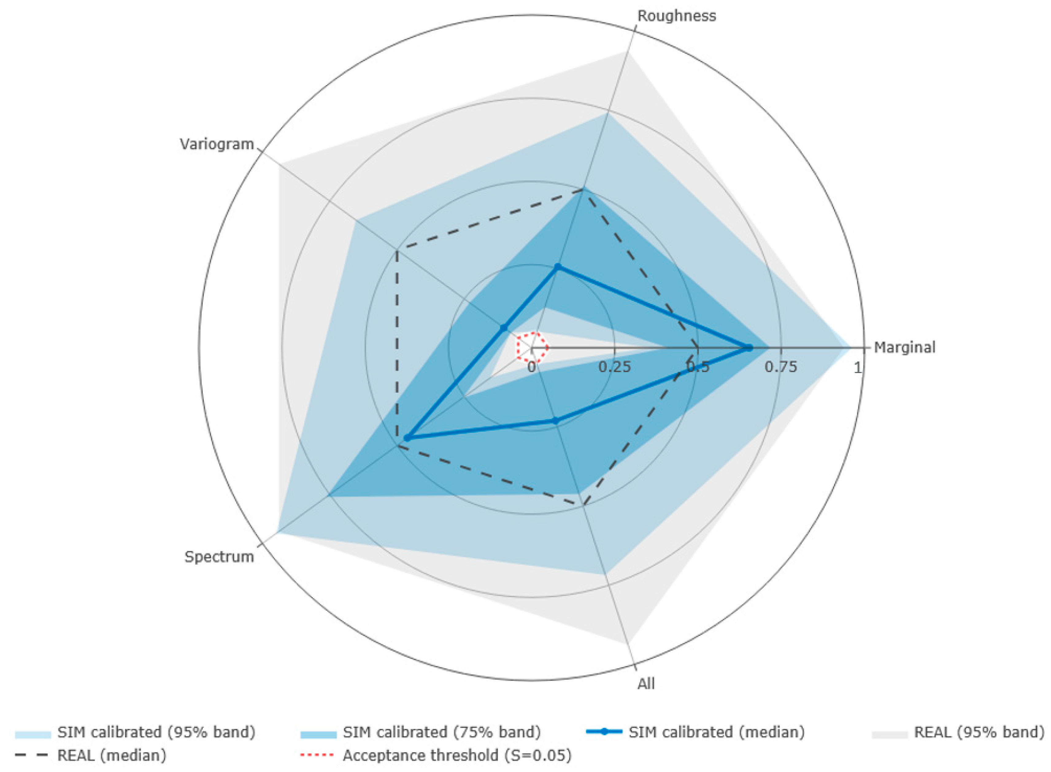
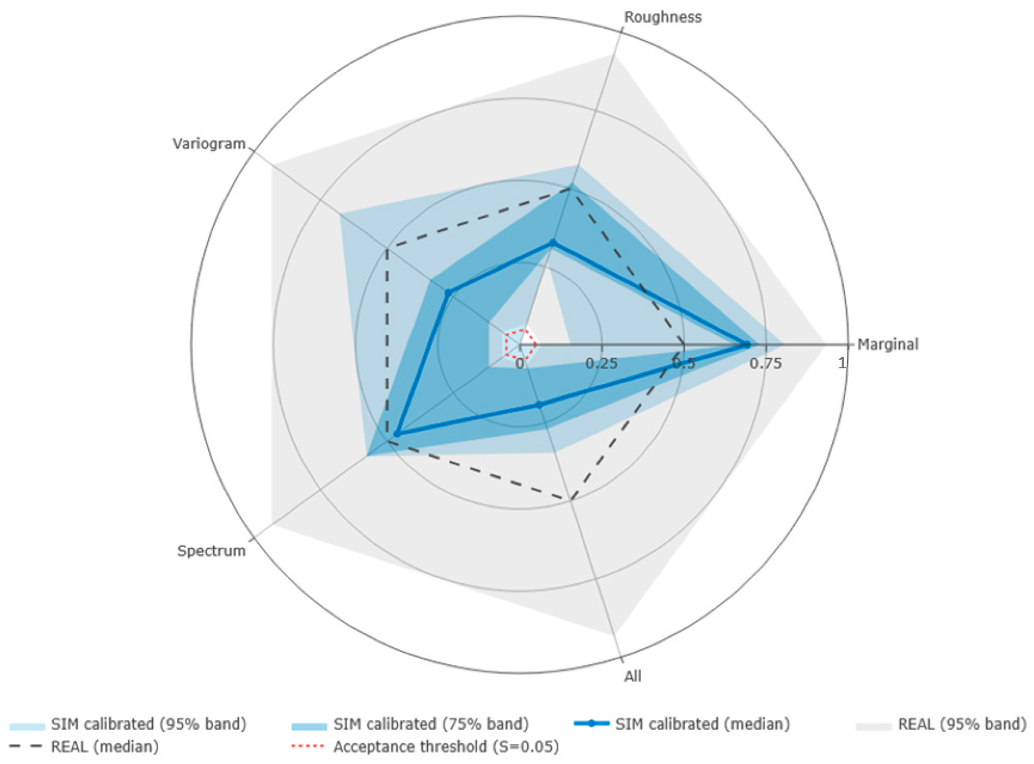
The variability observed across the available real cases provides an empirical statistical acceptance boundary, which makes it possible to assess whether a simulated raster can be regarded as a plausible realization of the same stochastic process that generated the real difference rasters, based on the descriptors introduced above. A simple Euclidean distance between feature vectors would not be fully adequate for this purpose, since it would not account for the non-negligible variability observed among real cases, nor for the correlations that inevitably exist among the different descriptors. Even a standardized Euclidean distance would compensate for the different numerical scales of the features but would still neglect their covariance structure. On the other hand, distribution-to-distribution metrics, such as the Wasserstein distance or the Kullback–Leibler divergence, would correspond to a different formulation of the problem, based on comparing two complete sample distributions, namely the real and simulated ones. Although such approaches may be useful when sufficiently large datasets are available, in the present case they would require a substantially larger number of real samples, especially considering the dimensionality of the feature vector, in order to provide robust and reliable estimates. This limitation is particularly relevant for metrics requiring an explicit estimate of a multivariate probability distribution or density. In this context, the Mahalanobis distance represents a suitable methodological compromise: it allows each simulated sample to be evaluated with respect to the empirical distribution of the real cases, while accounting for both the different variability of individual descriptors and the correlations among them. Therefore, in this work, the Mahalanobis distance is not interpreted as a parametric test based on the assumption of multivariate normality, but rather as an empirical compatibility criterion in feature space. Accordingly, the acceptance threshold is derived directly from the observed distribution of distances among real cases, rather than from a theoretical distribution.

The presence of non-Gaussian or heavy-tailed descriptors does not invalidate this empirical use of the Mahalanobis distance, but it affects how the resulting distances should be interpreted. In particular, $D^2$ values are not assigned a parametric probability under a multivariate normal model; they are used only to rank the relative departure of each sample from the empirical real-noise baseline. Nevertheless, strongly skewed or heavy-tailed descriptors may still affect covariance estimation and may produce unstable distance contributions, especially when the number of real samples is limited. For this reason, the final feature vector was intentionally kept compact and excluded descriptors that were found to be highly unstable or dominated by residual localized artefacts, such as kurtosis, extreme-value indicators, and overly high-dimensional curve representations. In addition, feature standardization, ridge-regularized covariance inversion, and per-feature contribution analysis were used to reduce numerical instability and to identify descriptors responsible for large distances. The sensitivity analysis reported in Appendix A further evaluates how the acceptance outcome changes when different empirical quantiles are used as thresholds.

Acceptance is defined by comparing $D^2$ against a threshold derived empirically from the real dataset. Rather than assuming a theoretical ${\chi }^2$ distribution (which may not hold due to non-Gaussianity), we compute the acceptance threshold as the chosen quantile $q$ of the $D^2$ values observed on the real samples themselves. A simulated sample is accepted if $D^2\le D_q^2$, meaning it falls within the variability envelope exhibited by real data in the selected feature space. In this study, the 95th percentile was adopted as the reference empirical acceptance threshold, as it provides a conventional compromise between retaining most of the variability observed in the real-noise baseline and excluding the most anomalous realisations. Since the threshold is derived empirically from the real samples, it is not interpreted as a theoretical confidence limit associated with a parametric distribution. A sensitivity analysis of this choice is reported in Appendix A.

For interpretability, we also compute per-feature contributions to the distance. Writing $\mathbf{p}={\mathsf{\Sigma }}_{\lambda }^{-1}\mathbf{z}$, the quadratic form can be expressed as $D^2={\sum }_j{z}_j\hspace{0.17em}{p}_j$. Ranking these contributions allows highlighting which specific descriptors contribute the most to the overall Mahalanobis distance (i.e., make the sample less stochastically compatible with the baseline model), providing useful insights on the possible elements that are not modelled appropriately by the simulator.

2.3. Proof of Concept with a Real-World Application

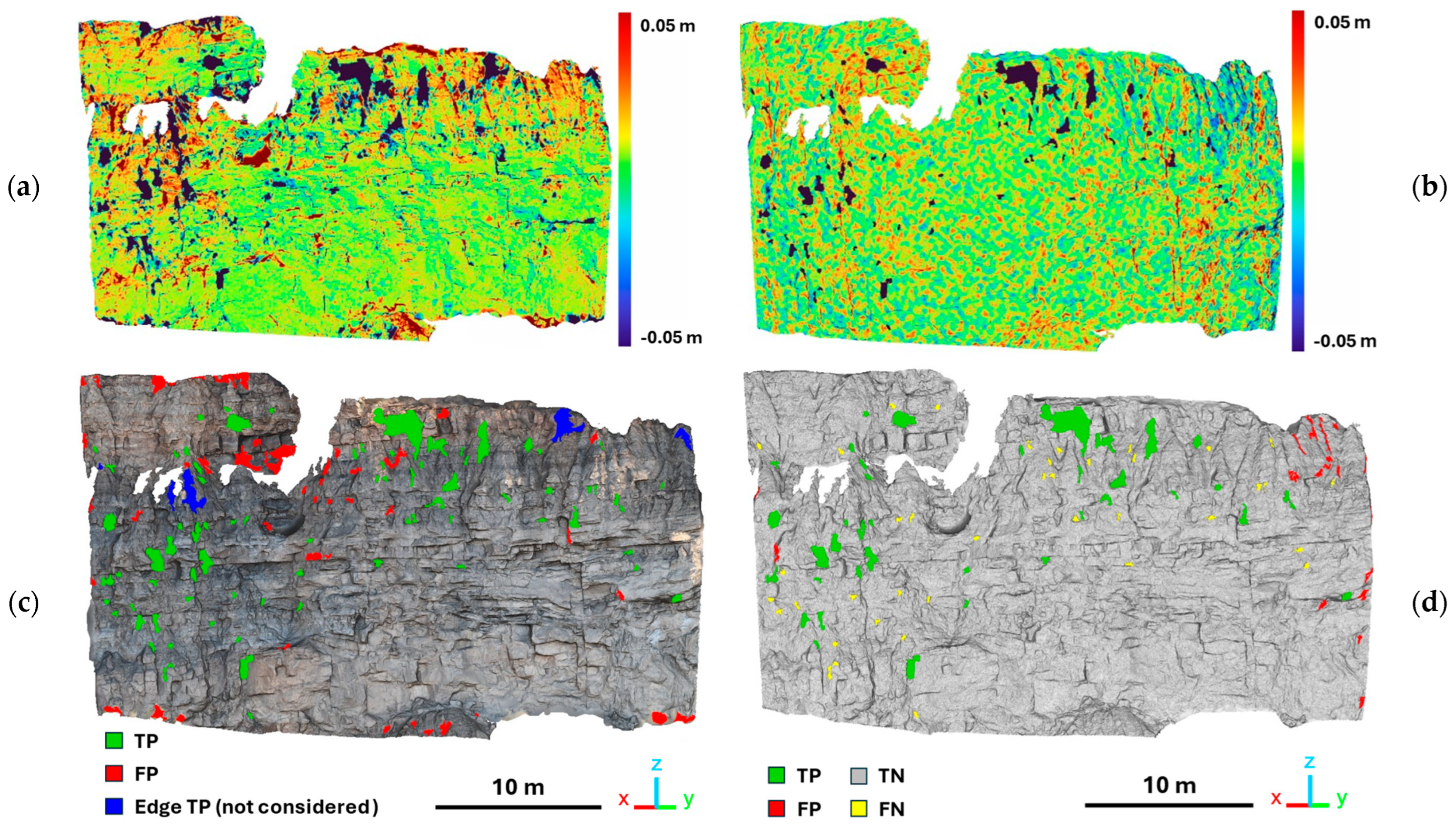
To demonstrate the applicability of synthetic rockfall data produced by the simulation methodology presented above to a real rockfall data scenario, two change detection analyses are performed and evaluated for a given rock slope. The first change detection analysis compares two real 3D rock slope mesh models from subsequent survey acquisitions of the same rock face, denoted the ‘reference’ and ‘comparison’ models, respectively. Identified changes are inspected by experts, manually labelling detections as true positive (i.e., detachments) and false positive (i.e., modelling artefacts) detections.

A third mesh model—denoted the ‘synthetic comparison’ model—is then generated by removing the verified detachments (i.e., specified blocks) from the reference model following the simulation methodology. To reduce uncertainty, any verified detachments along the edges of the real rock slope models (i.e., those partially within occluded areas or outside the monitored slope area) are not simulated. Calibrated noise parameters (Section 3.1) are also adopted, introducing photogrammetric noise to the synthetic comparison model. The second change detection analysis is then performed on this synthetic comparison model and the original reference model, generating a second set of changes. In this instance, the GT blocks provided by the simulation methodology are used to automatically label changes as true positive, false positive and false negative detections.

SlopeMonitor (SM [41]) is used for the change detection analysis. SM preserves the rock slope mesh texture, creating detachment volumes directly from the associated portions of the reference and comparison mesh models. Therefore, using SM ensures that the shape and texture of removed blocks in the synthetic comparison mesh model closely match those of real blocks. The algorithm implemented in SM is based on 2.5D raster differencing. For each comparison, the ‘comparison’ 3D model (point cloud or mesh) is first aligned to the ‘reference’ model using the ICP algorithm. Both 3D models are then compared to an inclined reference plane, creating a pair of 2.5D raster images with a user-defined resolution (pixel size). Each raster pixel contains the elevation of the rock slope model with respect to the reference plane, within the pixel area. A raster difference map is then generated by calculating the difference in elevation between corresponding pixels of the ‘comparison’ and ‘reference’ rasters. Within the corresponding difference map, negative differences represent material losses (detachments) and positive differences indicate accumulations or forward movements. Only pixels with negative differences are considered, as the focus is on rockfall detachments.

SM then applies a series of user-defined thresholds to filter out potential false detections coming from model uncertainties and isolate potential detachment clusters. First, any pixels with differences that are below a distance threshold are disregarded, forming clusters of neighbouring pixels with significant difference values (potential detachments). The value of this threshold typically corresponds to the 95th percentile of the normally distributed distance uncertainty of the rock slope models, derived from the registration error and surface roughness (LoD₉₅). Next, morphological filtering is applied, removing any clusters that do not satisfy specified minimum width and shape criteria. This filtering step can be performed over a number of iterations and is intended to remove artefacts and gross errors (e.g., very elongated change clusters due to model misalignment). Finally, an area threshold is applied to remove any change clusters that do not contain a minimum number of pixels. Despite several filtering steps, the remaining change clusters still need to be manually checked by experts to remove potential false positive detections. The volume of each remaining cluster is estimated by summing the volume of each cluster pixel (i.e., the product of the pixel area and difference in elevation).

2.4. Test Sites and Datasets

For simulator validation and for calibrating the noise levels so that they are consistent with those observed under real-world conditions, we relied on data acquired at two pilot sites.

2.4.1. Hunter Valley Test Site

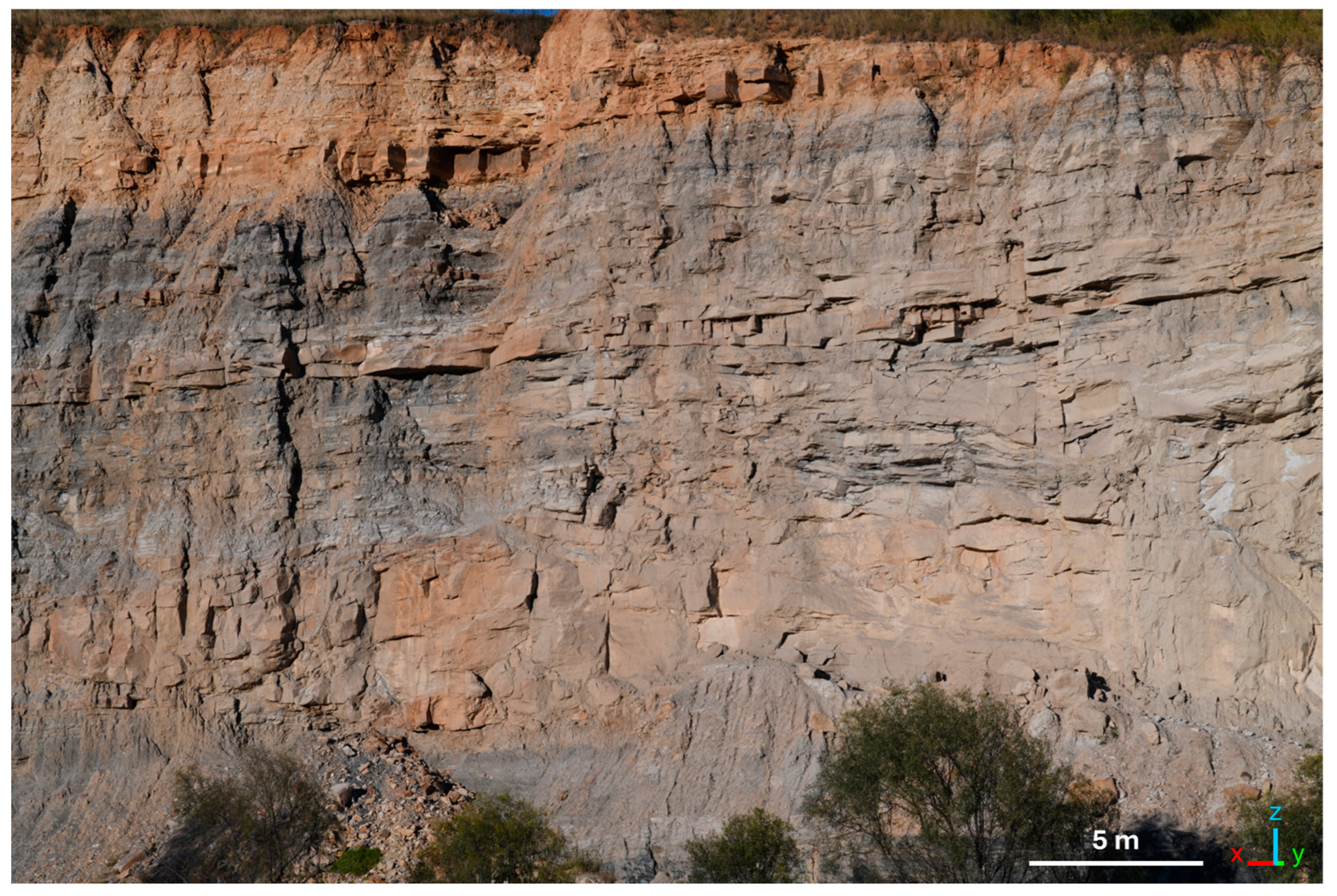
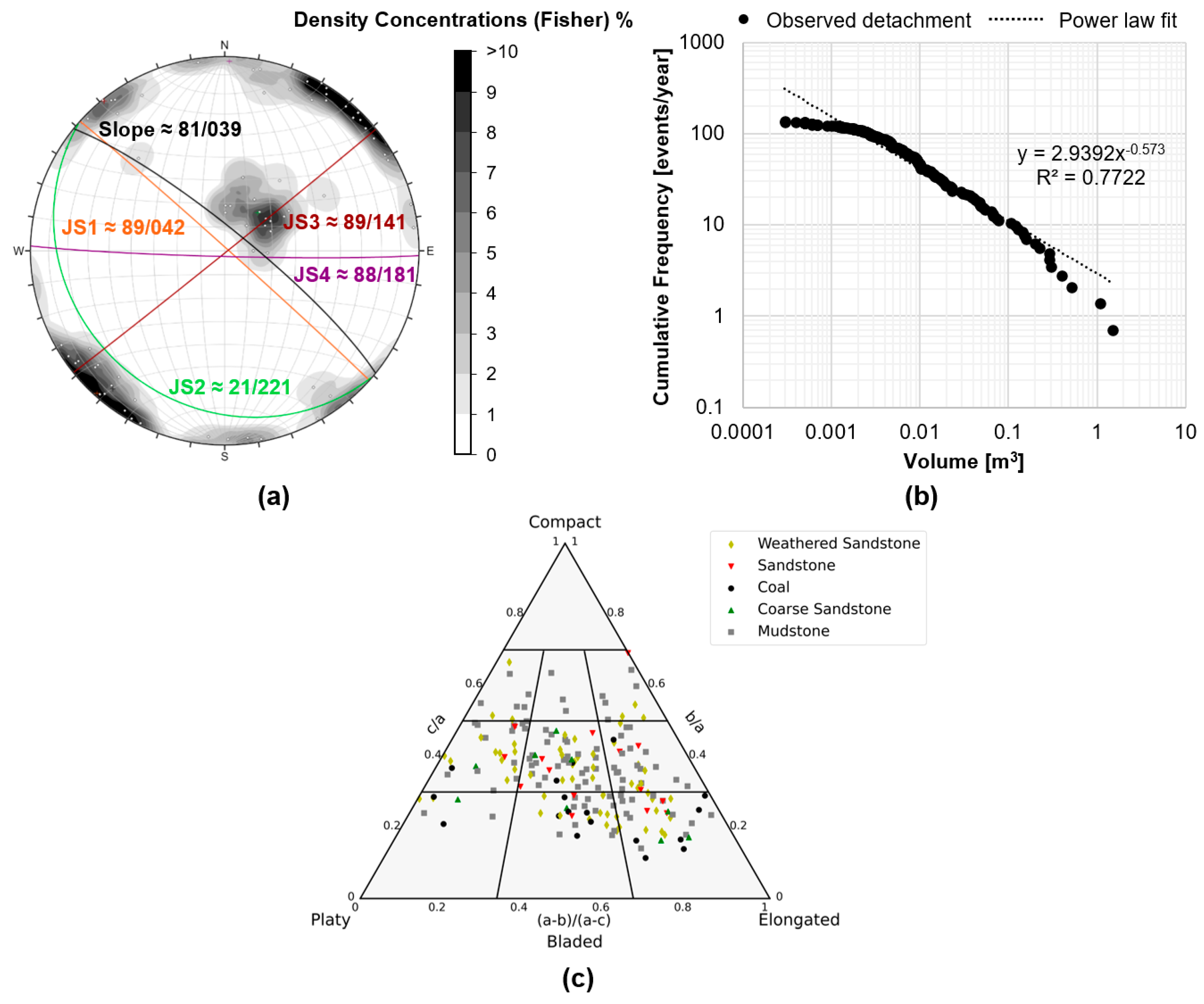
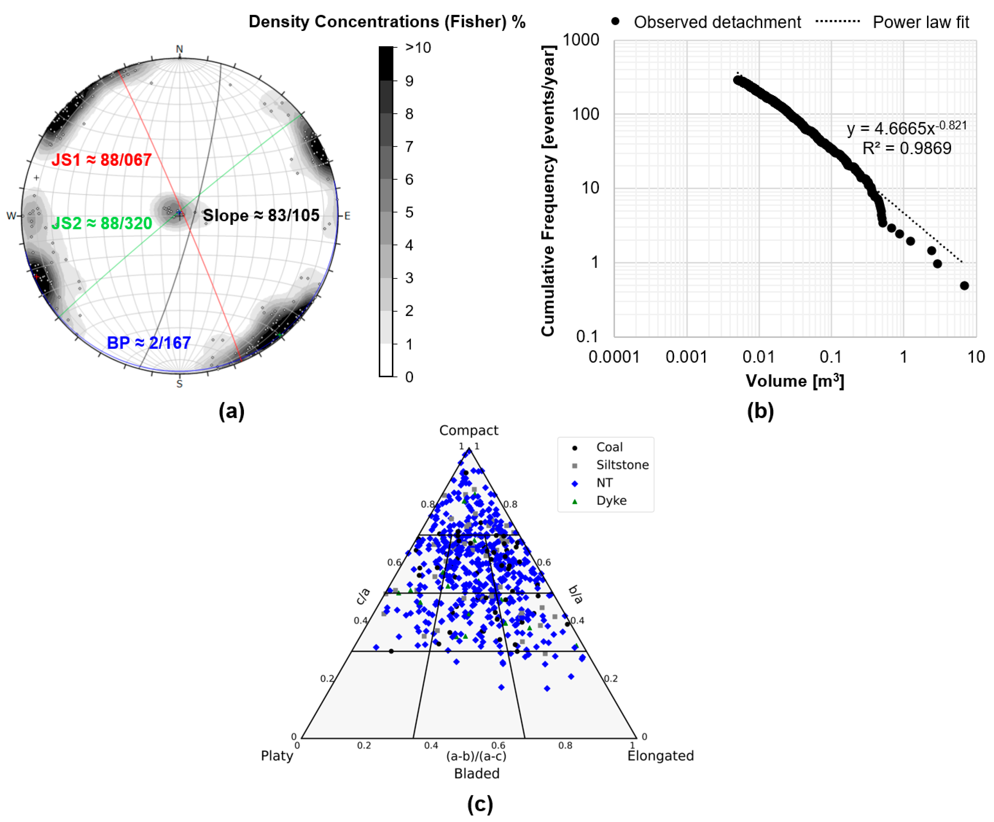
The first pilot site (hereafter referred to as HV) is located at an open-pit mine in the Hunter Valley (NSW, Australia). The rock face (Figure 5) is approximately 29 m high and 35.6 m wide. It is composed of five sedimentary lithologies (primarily sandstone, mudstone and coal). The four discontinuity sets observed across these geological strata tend to produce elongated and platy detachments (Figure 6).

Data were collected using the autonomous terrestrial stereo-photogrammetric monitoring system described in ref. [10], consisting of two stand-alone units specifically designed to detect volumetric losses from sub-vertical rock slopes in surface mining settings. Each unit is equipped with a full-frame Nikon (Tokyo, Japan) D850 camera (45.4 MP), fitted with fixed-focus optics (85 mm AF-S Nikkor (Tokyo, Japan) 85 mm f/1.8G lens). The two cameras were deployed at an approximate stand-off distance of 87 m from the rock wall, with a baseline of 32.6 m and a slightly convergent geometry to maximize image overlap. Under this configuration, the ground sampling distance (GSD) was 4.5 mm, and the depth precision (1σ) was estimated to be 6 mm.

The availability of a fixed photogrammetric monitoring system, installed on site for more than two years and acquiring data on a daily basis [44], enabled the creation of an exceptionally large dataset. This proved valuable both for calibrating and validating the simulator’s measurement-noise model and for assessing the simulator’s performance in an applied setting.

For noise validation, 39 inter-epoch comparisons were selected in which, based on an average observed LoD₉₅ of 6 cm, no rockfall events were expected to have occurred. In 30 cases, the two epochs used for comparison were very close in time (one day apart), whereas in others the temporal separation was larger (4–19 days apart). This limited the possibility for detachments below LoD₉₅ being considered as photogrammetric noise whilst also allowing for the exploration of noise across multiple durations. However, multiple statistical measures (Section 3.1) did not clearly distinguish between the single-day and multi-day comparisons, suggesting minimal contamination by potentially missed small detachments.

Each comparison was provided as a 2D raster of the differences with a spatial grid step equal to 1 cm.

For proof of concept (Section 2.3), a single comparison with user-defined blocks (directly from change detection on real data) was considered. This comparison spanned 34 days and yielded a significant number of detachments (as shown in Section 3.2). For Slope Monitor change detection, a spatial grid step of 2 cm (equivalent to four times the GSD) and a detection threshold of LoD₉₅ = 3 cm were adopted. A minimum square area of 4 cm by 4 cm was also set. Each detection size filter was applied over a single iteration.

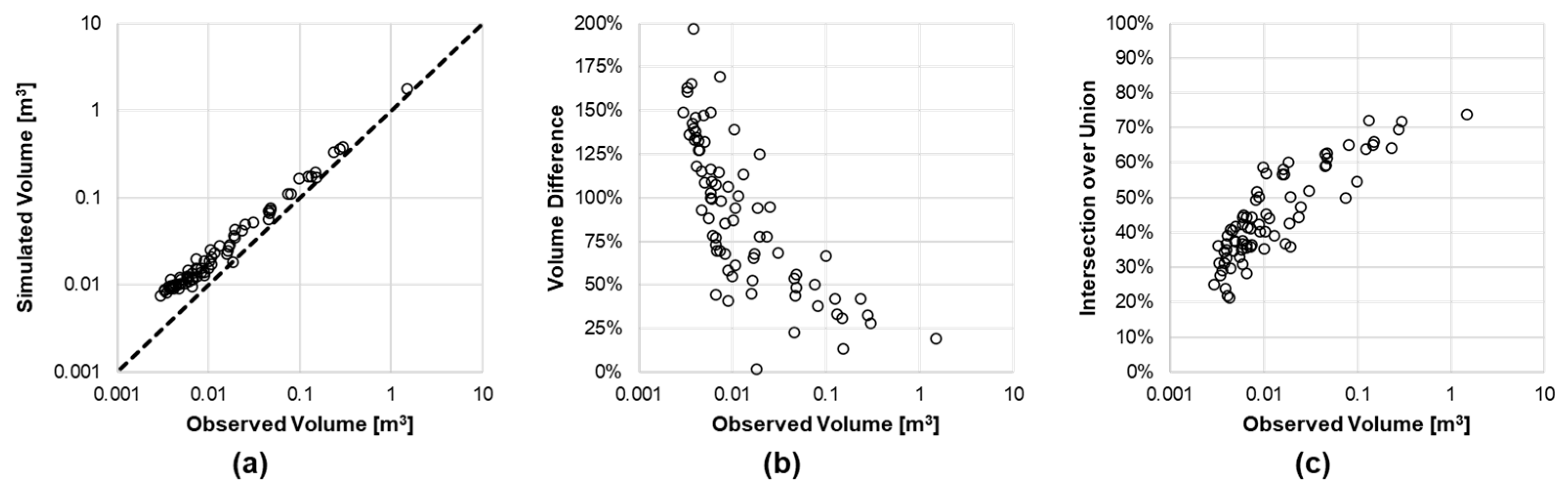
To further demonstrate the capabilities of the proposed simulation framework, ten additional synthetic change detection epochs were produced with randomly generated blocks. In this case, the size and shape of each randomly generated block were sampled directly from the distributions revealed via change detection on real rock slope monitoring data (Figure 6). Since the main joint set is oriented parallel to the slope surface, no orientation adjustments were applied. To represent discontinuity roughness, a surface irregularity distribution with zero mean and a standard deviation of 0.02 was assumed.

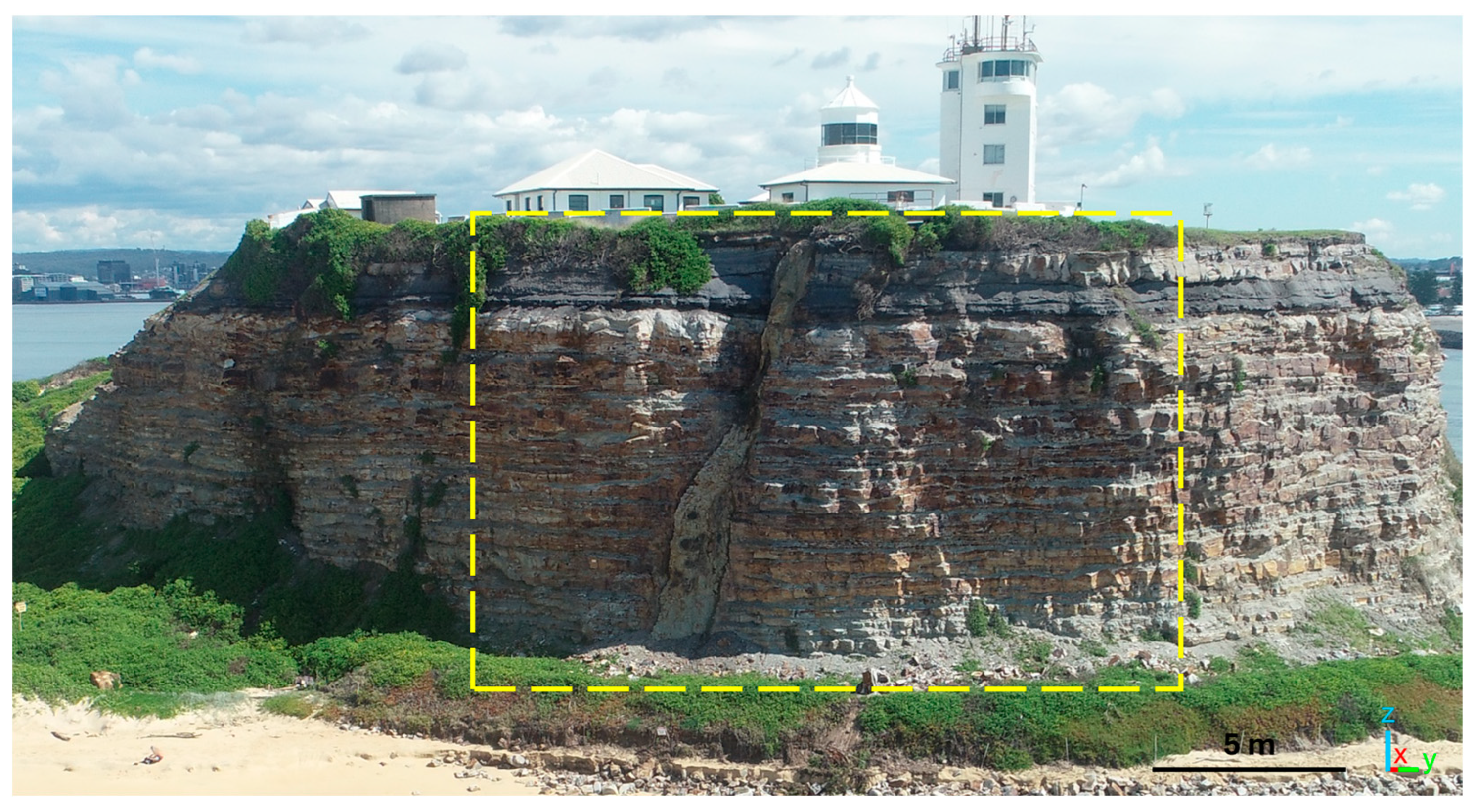
2.4.2. Nobbys Head Test Site

The second test site is a section of Nobbys Head, a circular coastal headland situated at the mouth of Newcastle Harbour, Australia (Figure 7). The cliff has long been associated with frequent rockfall activity, as indicated by the substantial accumulation of talus material around the base of the headland, repeated geotechnical investigations, and local Aboriginal knowledge [45]. A recent rockfall inventory study [2] further characterized the rock slope detachments from this site, using an inventory derived from two years of monthly photogrammetric drone surveys. The cliff comprises four main lithologies (primarily tuff, with coal, shale and a basaltic dyke) and the distinctly blocky surface texture is associated with the intersection of orthogonal, near-vertical joint sets and near-horizontal bedding planes. These geostructural features contribute to the frequent detachment of compact blocks (Figure 8).

These surveys were conducted using a DJI Phantom 4 RTK drone (Shenzhen, China) (8.8 mm/24 mm in a 35 mm format, f/2.8–f/11 lens), collecting 80 images (20 MP) via an automatic angled flight around 20 m away from the approximately 22 m high by 40 m wide area of the cliff face. The collected images were aligned using GNSS coordinates with real-time kinematic (RTK) positioning (i.e., no ground control points). This configuration resulted in a GSD of 5 mm and a depth precision of 15 mm (estimated as 3 times the GSD). Since the images from this site were processed using SfM photogrammetry (rather than classic stereophotogrammetry), the photogrammetric noise is expected to be different compared to the HV test site.

Unfortunately, the monitoring frequency in this case was much lower (monthly basis), and consequently, there were no comparisons without rockfall events. All 26 available monthly comparisons were therefore used for noise validation, but raster areas affected by validated detachments were masked before computing the noise descriptors. The masking was based on the expert-validated rockfall inventory obtained via non-parametric VoxFall change detection with a 0.05 m voxel size and systematic manual validation of each detachment cluster. This VoxFall analysis corresponds to a theoretical distance threshold of 0.1 m; however, expert validation did not rely solely on thresholded DEM differences. Systematic validation involved visual inspection of the 3D models and imagery, comparison with previous and subsequent surveys, identification of vegetation or transient objects, recognition of artefacts caused by misalignment or incomplete reconstruction, and assessment of areas affected by outliers or elevated uncertainty. Pixels belonging to the resulting mapped detachment areas were set to NaN before computing marginal statistics, variograms, spectral descriptors, roughness curves, and Mahalanobis-distance values. In this way, the dominant rockfall signal was excluded from the empirical noise baseline, and the validation analyses were restricted to portions of the rock wall interpreted as stable. Nevertheless, because very small changes may remain undetected, residual contamination of the real-noise reference set cannot be completely excluded and is acknowledged as a limitation of the NH calibration dataset.

3. Results

This section presents: (i—Section 3.1) the results obtained during the calibration of noise levels for both pilot test sites and the resulting validation of the simulator according to the methodology described in Section 2.2; and (ii—Section 3.2) a practical application of the simulator for benchmarking change detection approaches aimed at detecting detachment events. Accordingly, the first part assesses the stochastic compatibility of simulated data with respect to real measurements, whereas the second part illustrates an exemplary use case of the simulator in an applied benchmarking context.

3.1. Noise Calibration and Validation

To calibrate simulated measurement noise, we started by considering the uncertainty levels associated with the estimation of the different parameters. Bundle block adjustment (BBA) provides uncertainty estimates for the external orientation parameters (i.e., camera positions and rotations for the individual images) and, when on-the-job calibration is performed, also for the internal orientation and distortion parameters. In addition to per-parameter uncertainty values, BBA also enables computation of the covariance matrix describing how these parameters co-vary.

A separate discussion is required for the noise level associated with image matching. In this case, a direct uncertainty estimate cannot be readily derived. In general, for well-oriented imagery and well-textured surfaces, the matching uncertainty is expected to be below one pixel; however, this value is strongly case-dependent and influenced by the quality of the images and scene textures. An indirect indication could be obtained from the image-coordinate residuals of tie points identified during the SfM stage. Nevertheless, it must be noted that tie-point extraction relies on feature-based matching, which is fundamentally different from the area-based global or semi-global matching typically employed in dense MVS. Therefore, such residuals can at best be used as a proxy for overall data quality, but they cannot be assumed to directly represent the uncertainty affecting the dense-matching stage.

Finally, the proposed model for representing uncertainty in image matching (see Section 2.1.2) requires the calibration of three parameters: the local (pixel-wise) uncertainty, the noise associated with the regularization of the matching field, and the spatial scale (grid spacing) of that field. These parameters do not have a direct and unambiguous correspondence with real-world matching settings or with standard outputs provided by photogrammetric software and require tuning to be correctly expressed.

For this reason, a large number of simulated samples (difference rasters) were generated by the simulator while systematically varying the noise levels associated with each parameter (or parameter set). These simulated rasters were then compared, using the methodology described in Section 2.2, to the corresponding rasters derived from real data, with the dual goal of (i) assessing whether the uncertainty levels inferred from BBA produce realistic noise characteristics and, when this holds, (ii) identifying the parameter combination that yields the highest degree of agreement with real measurement noise patterns. The calibration was performed as a two-stage coarse-to-fine stochastic parameter search. In the first stage, a broad grid of plausible noise settings was explored to identify parameter intervals yielding low Mahalanobis distances. More specifically, the coarse search was defined in terms of multiplicative scale factors applied to the nominal noise levels adopted as the initial solution. For the EO/IO parameters, the nominal value was the uncertainty model derived from the BBA covariance matrix; the tested scale factors ranged from 0.75 to 1.50 of this nominal uncertainty level, with increments of 0.25. Equivalently, when the BBA covariance matrix was used, the perturbed EO/IO parameters were sampled using covariance matrices scaled as $s_{\theta }^2·{\mathsf{\Sigma }}_{BBA}$, with $s_{\theta }\in$ {0.75, 1.00, 1.25, 1.50}. The same multiplicative factors were used for the standard deviations of the local and regularized matching-noise components. The regularization scale of the matching field was explored independently over a broad range of candidate values, spanning approximately 15 to 100 pixels. This scale grid was not uniformly spaced; smaller scales were sampled more densely, whereas larger scales were tested with progressively coarser intervals, since the sensitivity of the resulting noise field was expected to decrease at larger regularization lengths. The objective of this coarse grid was not to perform an exhaustive deterministic optimization, but to identify the most promising noise-amplitude and regularization-scale intervals before the finer stochastic tuning of the matching-related parameters.

This stage should be interpreted as a structured parameter sweep rather than as a formal global optimization procedure, because each nominal parameter setting produces stochastic outputs and therefore potentially different $D^2$ values across repeated runs. The first stage indicated that, for both test sites, perturbing EO and IO parameters according to the covariance matrix derived from BBA provided the most compatible results among the tested alternatives. Therefore, in the second stage, these parameters were kept fixed at their BBA-derived uncertainty model, and only the matching-related parameters were varied around the most promising coarse intervals. Repeated simulations were performed for each nominal setting to account for the intrinsic stochastic variability of the simulator. This coarse-to-fine strategy was adopted for computational efficiency: it avoids an exhaustive search over all possible parameter combinations and concentrates the more expensive repeated simulations on the parameters that cannot be directly inferred from standard photogrammetric outputs, namely the local matching noise, the regularized matching noise, and the regularization scale.

For the HV site, the real dataset comprises 39 inter-epoch comparisons in which rockfall events are assumed to be minimal or absent. However, data inspection revealed that, in some cases, scattered vegetation, transient objects in the scene (e.g., people or, more frequently, animals), and local reconstruction issues in low-texture areas introduced non-negligible differences that would have substantially biased the overall characterization of measurement noise. Consequently, we filtered the difference rasters by removing outlier cells (setting them to NaN) when their absolute difference values greatly exceeded the expected depth accuracy, estimated at 1σ = 6 mm (see ref. [46]).

At the same time, the filtering threshold must be sufficiently high to preserve differences arising from imperfect co-registration between the pre- and post-epoch models. Based on preliminary tests, a threshold of 10 cm was adopted. This value effectively removes most outliers while retaining information associated with residual misalignment-induced differences.

Figure 9b–d shows three different examples of real-data difference rasters, all referring to the area identified in Figure 9a. The overall marginal distributions of the real rasters exhibit, in all cases, a mean value very close to zero (as a consequence of ICP-based co-registration), standard deviations ranging from 8.2 mm to 59.2 mm (the average standard deviation is 15.6 mm), and skewness values ranging from −1.05 to +1.44. Kurtosis values in the real cases are strongly variable (from −1.4 to 38.3) and are therefore not used in the final Mahalanobis-distance feature vector. This exclusion was adopted to avoid the acceptance test being dominated by a descriptor highly sensitive to residual localized artefacts and heavy-tailed behaviour.

Figure 10 shows the empirical envelopes of the real-data variability for the variogram (Figure 10a) and the multi-scale roughness curve (Figure 10b), computed as the 75th and 95th percentile bands across the full set of real difference rasters. For illustration, the corresponding curves of the three example rasters shown in Figure 9b–d are superimposed on the same plot, allowing a direct visual assessment of how individual realisations compare with the typical and upper-bound behaviour observed in real measurement noise.

Using the empirical 95th-percentile acceptance threshold for the $D^2$-based test gives a threshold of 24.9. The selected empirical acceptance quantile was assessed through a post hoc sensitivity analysis reported in Appendix A. Under this threshold, two out of the 39 real cases do not pass the acceptability test, as naturally expected. The largest contributions to increased $D^2$ values in the real cases are associated with the synthetic marginal distribution indicators and the values of the roughness and variogram curves.

As anticipated, the calibration of simulated noise can be considered as a coarse-to-fine stochastic grid search problem. Starting from an initial, plausible solution, namely one based on the uncertainty values estimated by the BBA and on noise levels commonly reported for the image-matching process, and given that the interactions among the simulator parameters are not known exactly, we seek to minimise the distance $D^2$ (or, equivalently, maximize the compatibility percentile) with respect to the real cases by varying the simulator noise levels. It is worth noting that, because measurement noise is generated stochastically, two simulations run with the same nominal noise settings may still yield different outcomes in terms of the resulting $D^2$. For this reason, we initially explored a broader and coarser range of noise-level variability (approximately 700 distinct simulations) in order to identify the most promising parameter intervals. This first stage revealed that the simulated outputs that most closely match the real data were obtained when the noise levels applied to the internal and external orientation parameters were set equal to those estimated by the BBA. For the matching-related noise, the coarse calibration indicated that the most suitable values were approximately $1\mathsf{\sigma }=0.6$–$0.8$ pixels, together with a relatively large regularization scale of about 50 pixels.

In a second stage, a more detailed fine-tuning was carried out. For the same nominal noise levels, multiple simulation repetitions were performed in order to account for the variability induced by the stochastic nature of the simulator. In this phase, an additional 200 simulations were tested by slightly varying the noise level and the regularization scale associated exclusively with the matching component. The noise levels and regularization scale were slightly changed accordingly (“best-fit” noise level) around the previously identified values.

Finally, 50 simulations were repeated using the same optimal noise configuration to quantify the percentage of runs that effectively pass the acceptance test. Figure 11 summarizes the results obtained. Only 4 simulations out of 50 showed out-of-threshold $D^2$ distances and have not passed the test. The acceptance rate (92%) is very close to the significance of the test (95%); therefore, within the adopted feature space and empirical Mahalanobis-distance test, the calibrated simulated noise is not distinguishable from the real-noise baseline.

The figure provides a compact representation of the degree of compatibility between the simulated rasters obtained with the “best-fit” configuration and the real data used as the baseline. Each axis reports the indicator groups considered separately (marginal statistics, multi-scale roughness, variogram, and power spectrum), as well as the “All” case, in which all indicators are jointly evaluated. The purpose of the plot is to highlight not only the average quality of the calibration, but also the variability across the 50 generated samples, while keeping the simulator parameters fixed at the “best-fit” noise setting.

For each sample, the squared Mahalanobis distance $D^2$ is computed (i.e., the squared distance from the typical behaviour observed in the real dataset). Since no theoretical distribution for $D^2$ is assumed a priori, the empirical distributions of real and simulated samples are analysed. For each indicator group, the empirical cumulative distribution function ${\widehat{F}}_{\mathrm{real}}\left(D^2\right)$ is constructed from the real cases, and each simulated realization is evaluated in terms of its “compatibility percentile” with respect to the baseline. Accordingly, the radar plot reports, on each axis, a normalized score defined as $S=1-{\widehat{F}}_{\mathrm{real}}\left(D^2\right)$. This quantity lies in the interval $[0, 1]$: higher values indicate that the simulated sample falls within the most compatible portion of the real distribution (i.e., it exhibits a small $D^2$ relative to the baseline), whereas values close to zero indicate samples that are “farther” from the baseline than the real cases themselves. In the figure, the acceptance threshold corresponding to the 95th percentile criterion on the real data translates into $S=0.05$, represented by the central red dashed region.

The figure also reports the median simulated-score profile (blue line), together with two envelopes capturing variability: a wider band corresponding to the 95th percentile (light blue) and a narrower band (dark blue) corresponding to the 75th percentile. Of the two, in Figure 11, the 75th-percentile envelope is relatively tight, indicating that, under fixed simulator parameters, the stochastic process generates coherent and stable samples. It is also noteworthy that, for the marginal-distribution statistics, the identified “best-fit” noise setting yields consistently strong performance, with simulated samples generally closer to the baseline than individual real cases. In terms of the power-spectrum distance distribution, simulated samples appear consistent with the empirical distribution obtained from real data. Slightly less favourable, yet still fully acceptable, results are observed for the variogram and roughness descriptors, which may suggest that while the noise amplitude is properly captured, the spatial correlation structure and possible localized discrepancies are not yet modelled optimally. Finally, the “All” axis provides a synthetic measure of overall agreement: a high and stable value of $S$ on this axis indicates that the calibrated configuration consistently reproduces not only the marginal distribution of errors, but also their multiscale spatial structure, as captured by roughness, variogram, and spectral descriptors.

As for NH, the second test site (Figure 12), the validation and calibration procedure essentially followed the same workflow adopted for the previous case.

However, as can be observed by comparing the rock-face morphology and the noise patterns in Figure 12 with those in Figure 9, the two case studies exhibit markedly different characteristics. The NH test site is characterized by discontinuities that are both more pronounced and more densely distributed in space. Moreover, because the rock face was surveyed using multiple UAV flight strips with strong overlap in both longitudinal and transverse directions, the measurement noise is substantially more uniform (i.e., the distinctive random structures clearly visible at the HV site are, here, only weakly present) and its magnitude is generally lower. Finally, because the camera viewpoints are very likely not identical from one epoch to the next (even though the UAV acquisition is planned on the same nominal flight plan), occlusions and sharp geometric discontinuities produce much more evident artefacts in inter-epoch comparisons than in the previous case. Even from a purely visual inspection, it is apparent that the two selected sites exhibit significantly different noise characteristics.

The overall marginal distributions of the real rasters exhibit, in all cases (and as in the previous test site), a mean value very close to zero, strong kurtosis variability, standard deviations ranging from 8.3 mm to 16 mm (average standard deviation is 11 mm), and skewness values ranging from −2.26 to +1.24. As for the HV site, kurtosis was not retained in the final Mahalanobis-distance feature vector because of its instability and sensitivity to localized artefacts. In this second test, the variability of the difference values is much more limited, as the visual inspection has already hinted. Using the empirical 95th-percentile acceptance threshold for the $D^2$-based test gives a threshold of 10.4. Under this threshold, two out of the 26 real cases do not pass the acceptability test. The largest contributions to increased $D^2$ values in real cases are associated with the synthetic indicators of the marginal distribution and with the variogram curves.

Although the simulator would in principle allow the same photogrammetric block to be reproduced, the use of a large number of images (each of which would need to be simulated individually) would lead to computational costs that are currently prohibitive, at least in the present implementation of the simulator. Therefore, simulations were performed using a simplified photogrammetric block configuration (i.e., analogous to that adopted for the HV site). This choice, however, makes the calibration of noise levels more challenging, as it requires exploring a substantially broader range and a larger number of parameter combinations to reproduce the effective noise characteristics observed in the NH dataset.

Also, for this test site, a first, broad tuning using approximately 600 distinct simulations was implemented, identifying the most promising parameter levels. However, some useful indications coming from the previous test-site experiment (e.g., using the estimated internal and external orientation parameter uncertainties) confined the search space and allowed for identifying, in this first tuning round, the “best-fit” configuration. For the matching-related noise, the optimal configuration corresponded to values approximately $1\mathsf{\sigma }=0.6$ pixels, together with a smaller (if compared to the optimal one identified for the HV test site) regularization scale of about 26 pixels.

Finally, as in the previous case, 50 simulations were repeated using the same optimal noise configuration to quantify the percentage of runs that effectively pass the acceptance test. Figure 13 summarizes the results obtained.

In this case, although the simulations reproduce the marginal distribution of the measurement noise and provide a credible representation of its roughness, they are less successful than in the previous case study at replicating the spatial correlation structure, as described by the variogram, and the spectral characteristics observed in the real noise fields. When repeating the $D^2$ test while restricting the feature vector to the variogram-related components only, or to the spectrum-related components only, the corresponding acceptance rates are 82% and 90%, respectively. Overall, considering the full feature vector (i.e., considering simultaneously marginal distribution, roughness, variogram and spectrum), only 39 simulations (out of 50) were actually accepted by the $D^2$ test. This lower acceptance rate, most likely, should be interpreted in light of the deliberately simplified acquisition geometry used for NH: the test therefore represents a more challenging transfer case rather than a reproduction of the original UAV block.

Table 1. Summary of the two validation datasets, best-fit simulator noise settings, and empirical acceptance-test results. The D² threshold corresponds to the 95th percentile of the real-noise feature-space distances, while acceptance rates are computed from 50 repeated simulations using the calibrated best-fit configuration.

	HV Test Site	NH Test Site
Site and real-acquisition characteristics
Size	35.6 × 29 m	40 × 22 m
Image block geometry	Stereo-pair	Oblique UAV 80 × 80 strip block
No. of images	2	80
GSD	4.5 mm/pixel	5 mm/pixel
Camera/sensor	DSLR-Full Frame Nikon D850 (45.4 MP)	Integrated UAV camera 1″ CMOS (20 MP)
Simulation setup and best-fit noise settings
Simulated img. block geometry	Stereo-pair (reproduced)	Simplified stereo-pair (as HV)
EO parameters	Multivariate Gaussian using BBA covariance matrix	Multivariate Gaussian using BBA covariance matrix
IO parameters
Pixelwise matching noise	Gaussian—s = 0.7 pixel	Gaussian—σ = 0.6 pixel
Regular. matching noise	Gaussian—s = 0.7 pixel	Gaussian—σ = 0.65 pixel
Regular. scale (Matching)	50 pixels	26 pixels
Empirical validation outcome
No. of real comparisons	39	26
$D^2$ acceptance threshold	24.9	10.4
Accepted simulations	46/50 (92%)	39/50 (78%)

summarizes the main characteristics of the two test sites and acquisition configurations, together with the best-fit noise parameters adopted in the simulator and the corresponding empirical validation results. The comparison highlights the different complexity of the two calibration scenarios: the HV dataset is based on a terrestrial stereo-pair configuration that can be directly reproduced by the simulator, whereas the NH dataset derives from a more complex UAV multi-image block, which was approximated using a simplified photogrammetric configuration for computational reasons. Consistent with this difference, the calibrated HV simulations achieved an acceptance rate close to the nominal 95% criterion, while the NH case showed a lower but still substantial acceptance rate, mainly reflecting the greater difficulty of reproducing the spatial correlation and spectral structure of the real noise field.

3.2. Proof of Concept with a Real-World Application

The first change detection analysis (as described in Section 2.3 and Section 2.4.1) identified 77 true positive (i.e., detachments) and 43 false positive changes across the HV rock wall within an approximately one-month monitoring period (Figure 14a,c). The simulation methodology successfully generated a synthetic comparison model (Figure 14b), removing the same 77 detachments and applying the calibrated noise parameters discussed in Section 3.1. As previously mentioned, the five detachments on the edges of the model were not included in this simulation. The subsequent (second) change detection analysis and comparison with GT data revealed true positive, false positive, and false negative changes (Figure 14d).

From a visual comparison of the real (Figure 14c) and simulated (Figure 14d) changes detected by the SM configuration, the positions and shapes of simulated blocks appear to be consistent with real observations. Quantitative comparisons of the observed volumes with the corresponding simulated GT volumes (Figure 15a,b) revealed that the simulation framework systematically overestimated the observed volumes. This overestimation was slight (<50%) for larger blocks and significant (up to 200%) for smaller blocks. Considering how well the volume of each GT block overlaps with the corresponding observed volume (via an estimated Intersection over Union ratio), it showed that the position of smaller GT blocks is also less consistent with the position of each observation compared to larger volumes (Figure 15c). These disparities are understandable, considering how the proposed framework places and removes specified blocks. As input block volume decreases, the associated block dimensions approach the average distance between vertices for the input slope mesh. This makes it more difficult to remove blocks and satisfy the necessary geometric, numerical, and topological constraints (as mentioned in Section 2.1.1) without adjusting their positions. Note that an overestimation of 200% implies that the input block had to be extruded to two times its original depth in order to be properly removed.

Whilst the differences between corresponding real and simulated blocks are significant, they would only be a concern when trying to exactly reproduce the characteristics (i.e., volume, position and shape) of user-defined blocks. This would include trying to achieve a particular block volume distribution. As potential differences are related to the resolution of the input slope mesh, increasing this resolution would reduce differences in blocks with smaller volumes. However, if a sufficiently high resolution is not attainable, only larger blocks can be replicated. It should be noted that most applications of the framework (e.g., change detection analyses) only require synthetic rockfall geometries that are equivalent to—not exactly the same as—real rockfalls. Therefore, this limitation should not be a concern in most cases.

This application of the simulation framework to a real change detection analysis case demonstrates several advantages of having GT data for rockfall detection. The proportions of false positive detections for each change detection analysis are very similar (precision values: 65.6% for real data and 66.7% for synthetic data). However, the time required for identifying and removing these false positive detections from the respective detachment inventories is not equivalent. Manual checking for the real dataset was in the order of four hours, while checking with GT data for the synthetic dataset is almost instantaneous. While many performance measures can be estimated for the synthetic case (e.g., recall, accuracy, F1-score), the real case lacks the necessary values for these estimates. Therefore, the GT data generated by the simulation methodology facilitates a more comprehensive assessment of the adopted change detection approach.

The comparison with GT data (Figure 14) also highlights that detachments can be missed during change detection (false negatives), often due to data resolution and parametric limitations (e.g., limit of detection). Additionally, while the certainty of the detachment volume estimates from real data is unknown, the comparison with GT data revealed that volume estimates differ by 48% on average from the target value, for this change detection analysis (Figure 16). This GT comparison suggests that the particular SM analysis scenario tends to systematically underestimate detachment volumes. In other words, the observed average volume deviation should not be interpreted as an error in the synthetic GT itself, but as the discrepancy between the known removed volume and the volume recovered by the adopted change-detection workflow (SM). Several factors may contribute to this difference: the LoD₉₅ threshold removes low-magnitude pixels, especially near detachment margins; morphological and area filters may fragment or discard parts of small detachments; the 2.5D raster representation approximates a fully 3D surface change on an inclined reference plane; and simulated photogrammetric noise, residual co-registration effects, and local occlusions may alter the reconstructed detachment boundaries. The result therefore illustrates the diagnostic value of synthetic GT: it makes it possible to quantify volume-estimation errors that would remain unknown in a purely real-data comparison.

Additional SM analyses on ten synthetic epochs (with randomly generated blocks) provide further evidence for systematic volume underestimation (Figure 17). The volume difference and Intersection over Union values do not appear to correlate with GT volumes. Therefore, the significant volume differences are due to the threshold distance set within SM. Any block areas (i.e., raster pixels) with distances below this threshold value are not included in volume estimates, leading to systematic underestimation. Changes in model alignment during ICP registration, due to the presence of noise, can further exacerbate or reduce this effect.

Across the ten synthetic epochs (i.e., 1000 blocks), an average precision of 56.7% and recall of 24.4% were observed, resulting in an average F1-score of 34.1%. Like in the initial representative monitoring period, the distance threshold and model misalignment continue to impact the detectability of randomly generated blocks. There is a clear separation in the volume range of detected and GT blocks, but not in the shape classes (Figure 18). GT blocks below 0.003 m³ were not detected, resulting in a much steeper magnitude-cumulative frequency relationship (Figure 18a). The undetected blocks (FN in Figure 18b) are quite spread, with a concentration in the very blady section. Because there is a similar concentration of detections (TP), and the input distribution was also skewed towards the blady and very blady sections, these analyses do not necessarily suggest that more extreme geometries, such as very blady, are more likely to be missed by this SM configuration.

Comparison of the procedurally generated GT block volume and shape distributions (Figure 18) with those from real change detection observations (Figure 6) provides further insights on the behaviour of the proposed simulation framework. While the shape distributions (Figure 6c and Figure 18b) have similar tendencies towards blady and very blady classes, the simulated magnitude-cumulative frequency relationship (Figure 18a) has more pronounced tails compared to the input volume distribution (Figure 6b). Since the minimum input volume class was 0.0001–0.001 m³ (in line with real observations), the roll-over effect for volumes below 0.0001 m³ is consistent with how the proposed simulator removes blocks from the original rock slope mesh model. For successful removal, each block must be split by the intersection with the slope mesh. Therefore, by definition, the GT block volumes will always be smaller than the input block volumes. Due to variations in block shape and the local orientation of the rock slope (i.e., roughness), the ratio between GT and input block volumes is not constant and cannot be systematically adjusted. The extreme effect can be similarly understood: the splitting of blocks with larger volumes reduces the corresponding cumulative frequencies. However, the significant increase in overall curvature is due to both block splitting and the previously observed tendency to shift (or reject) smaller blocks in order to satisfy the geometric, numerical and topological constraints imposed within the simulator. In general, a smaller block is more likely to be shifted until its depth is sufficient for valid removal, increasing the removed proportion of the block volume (i.e., GT volume). Conversely, a larger block is more likely to be accepted for removal without shifting, increasing the likelihood of a smaller GT volume. Both extremes tend to produce GT volumes that are towards the middle of the input volume range (e.g., 0.01 m³), increasing the curvature of the magnitude-cumulative frequency relationship.

Whilst additional block removal acceptance criteria could be imposed within the simulator to reduce the instances of blocks below the input minimum volume (roll-over effect), this would not reduce the extreme effect nor the curvature of the volume distribution. Similarly, scaling the input volume distribution might produce a similar range of GT volumes, but it would not address the other disparities, especially for complex block and slope geometries. As previously mentioned, increasing the resolution of the input rock slope mesh model could reduce the tendency to shift smaller blocks, reducing the overall curvature. If the necessary resolution is not achievable, and a particular GT volume distribution shape is required, the volume range should be limited to larger values. This would ensure sufficient initial block depths, according to the input mesh resolution. However, as the most likely application of the simulator—testing change detection analysis configurations—does not require the exact replication of rockfall volume distributions, the observed differences between real and simulated data do not discount its usefulness.

As previously observed, simulating and testing the blocks observed via real change detection analyses can lead to significant volume differences and limits the subsequent analyses to a specific range of block sizes and shapes. Additionally, the input block set is biased, as only blocks that are above the limit of detection and manually validated by an expert technician are considered. The possibility to create additional synthetic epochs via random block generation greatly reduces this bias and facilitates a more comprehensive assessment of change detection performance. The simulation framework also enables multiple noise scenarios to be considered, providing further insights into possible performance. For example, the impact of changing camera position on the quality of change detection data could be explored, informing future survey plans. Therefore, the proposed framework allows change detection configurations to be tested with characteristics beyond what has been previously observed within real rock slope monitoring.

4. Discussion

It is important to clarify that the proposed simulator does not aim to reproduce the full physical process of rock mass failure, which would require multi-physics modelling of stress propagation, fracture initiation, and material heterogeneity, which is only partly considered with user-defined block removal. A formal quantitative assessment of realism remains a challenging and open problem in simulation-based dataset generation and is beyond the scope of this work.

Instead, the simulator is designed to generate geometrically and statistically plausible post-failure morphologies that are consistent with known geotechnical constraints and observable outcomes of real detachment events. This choice reflects a deliberate trade-off between physical completeness and controllability of the ground truth, which is essential for algorithm training and validation.

A similar scope distinction applies when comparing the proposed framework with physics- or game-engine-based rockfall runout simulators, such as the fragmental rockfall simulations based on TLS-derived rockfall inventories reported in ref. [21]. Such approaches primarily aim to reproduce the post-detachment motion, propagation, and interaction of detached fragments. In contrast, the present framework does not attempt to simulate runout dynamics, but focuses on generating known pre-/post-failure surface changes on the monitored rock face and on reproducing the measurement noise affecting photogrammetric change-detection products.

At the same time, to mitigate the risk of embedding strong simulator-specific priors, the generation process is explicitly stochastic and highly parameterized. Block geometry, surface roughness, orientation, scale, and spatial distribution are not fixed but drawn from configurable probability distributions, including user-defined densities. This design allows the generation of a broad family of plausible morphologies rather than a narrow set of canonical cases, reducing the likelihood that downstream models overfit simulator artefacts.

The results reported in Section 3 confirm that, after site-specific calibration, the simulator is able to realistically represent several key characteristics of measurement noise and that its use in applied settings can effectively provide outcomes comparable to those that would be obtained using a (much more demanding) approach based on real data and manual rockfall mapping. The validation of the simulated measurement noise remains the most delicate step of the overall procedure and, for some applications, it may represent the crucial element for supporting a reliable testing methodology. Nevertheless, based on the two case studies here analysed, this phase cannot be conducted without a preliminary tuning of the noise levels. As extensively demonstrated, calibration cannot rely on pointwise comparisons between real and simulated difference rasters, but must instead be based on statistical descriptors computed over a sufficiently large number of repetitions. Even a purely visual comparison of the noise patterns in the real cases shown in Figure 9 and Figure 12 highlights the highly stochastic nature of the problem.

In this context, the Mahalanobis-distance acceptance model should therefore be interpreted as an empirical compatibility test rather than as a formal parametric hypothesis test. Its robustness depends on several safeguards adopted throughout the workflow: unstable descriptors are excluded from the final feature vector, the covariance inversion is ridge-regularized, thresholds are derived empirically from real-data distances, and repeated simulations under fixed best-fit parameters are used to quantify the variability induced by the stochastic simulator. These choices do not eliminate the effect of non-Gaussian descriptor distributions, but they reduce the risk that the acceptance decision is dominated by isolated heavy-tailed features or by numerical instability in the covariance estimate.

However, the need for a large number of repeated real measurements is also the main limitation for extending the tuning methodology to additional sites. While it is reasonable to expect that fixed monitoring systems will become more widespread (thus enabling the collection of extensive datasets for tuning and validation), to the authors’ knowledge, only a limited number of case studies (mostly within dedicated research activities) provide multi-epoch datasets with a sufficiently high number of repetitions to support a methodology comparable to that presented in this work.

Despite this limitation, the two calibrations performed here yield a methodologically relevant finding: the uncertainty levels of the internal and external orientation parameters estimated by BBA, in the two test cases analysed, are sufficient to make the simulator consistent with real data without requiring ad hoc tuning. This supports the idea that the “geometric” components of the photogrammetric pipeline (EO/IO) can be inferred directly from standard photogrammetric estimation outputs, whereas dense matching introduces additional degrees of freedom that indeed require explicit calibration. This calibration should not be interpreted as a validation of the internal mechanics of a specific dense-matching algorithm. Rather, it indicates that the simplified disparity-noise model can reproduce, at the DEM-difference level, the output noise statistics most relevant for the present benchmarking task, while algorithm-level simulations including texture, illumination, and radiometric artefacts remain outside the scope of this work. A related limitation is that the current simulator does not explicitly model scene-level and radiometric disturbances such as vegetation changes, moving objects, cast shadows, illumination changes, surface wetness, dust, motion blur, etc. These factors can affect photogrammetric change detection in different ways: vegetation and transient objects may introduce occlusions or apparent surface changes; shadows, illumination variations, and surface wetness may alter image texture and matching reliability at the local level; motion blur may reduce local image sharpness and increase reconstruction artefacts. In the present framework, some of their aggregate effects may be indirectly reflected in the empirical real-noise baseline used for calibration, or removed in the real dataset used for validation through masking and outlier filtering when they generate clearly localized artefacts. However, they are not controlled independent variables of the simulation. Consequently, synthetic datasets generated with the current framework are most appropriate for benchmarking geometry-driven change detection under calibrated photogrammetric uncertainty, whereas applications involving strongly variable vegetation, lighting, or image-quality conditions may require additional disturbance modelling or domain-randomization strategies.

At the HV site, where the simulated acquisition configuration (a single stereo-pair) matches the real one, the calibration achieves strong compatibility with real measurements according to the adopted statistical descriptors. Using an empirical threshold for the $D^2$ test at the 95th percentile (HV: threshold 24.9) leads, as expected, to a small number of real realisations classified as “anomalous” (2 out of 39). The set of 39 real comparisons provides a sufficiently broad baseline to characterise the empirical variability of the measurement process. The robustness experiment based on 50 simulated repetitions under fixed “best-fit” parameters yields an acceptance rate of 92% (4 “anomalous” simulations out of 50), consistent with the 95th-percentile criterion adopted to define the acceptance threshold on the real dataset. Therefore, for Site HV, the simulator generates data that are stochastically indistinguishable, at least according to the adopted metrics, from those expected under real measurement conditions.

At the NH site, the same workflow was applied, but noise tuning did not achieve the same level of agreement observed for HV. In this case, the real baseline is narrower (24 repetitions of real acquisitions), which contributes to a lower empirical acceptance threshold for the $D^2$ test (10.4). In addition, scene and acquisition characteristics (more pronounced discontinuities, strong UAV overlap, and non-identical viewpoints across epochs) produce noise that is overall more uniform and of smaller magnitude, yet with more evident comparison artefacts near discontinuities and occluded regions. Finally, the use of a simplified photogrammetric block geometry in the simulations (for computational reasons) makes it more difficult to faithfully reproduce the spatial signature of the noise: the results indicate that the calibration reproduces the marginal distribution and the roughness well, but more frequently fails to replicate the spatial correlation structure (variogram) and the spectral characteristics. When repeating the $D^2$ test while restricting the feature vector to the variogram-related components only or to the spectrum-related components only, the corresponding acceptance rates are 82% and 90%, respectively. This clearly indicates that the mismatch is not dominated by a single descriptor, but rather arises from the interaction among multiple statistical properties when they are jointly evaluated. The overall acceptance rate (slightly below 80%) is nevertheless satisfactory, considering that the simulations are based on a significantly different photogrammetric block geometry and that the rock-slope morphology poses substantially higher challenges for accurate reconstruction. In particular, the NH results show that calibration can remain “acceptable” even when the simulated acquisition block is simplified, although this entails a reduction in overall acceptance (~78%), reflecting the difficulty of fully reproducing the observed spatial structure of the noise.

This outcome does not invalidate the simulator; rather, it clearly delineates its current domain of applicability while suggesting directions for improvement. For multi-image scenarios (e.g., UAV blocks) or geometrically complex settings with significant viewpoint variability, reproducing the spatial structure of measurement noise likely requires either (i) a more faithful simulation of acquisition geometry (number and distribution of images) or (ii) a noise model capable of incorporating occlusion effects and spatial anisotropies. Of these two, the first option will be further investigated in the future (improving the computational efficiency of the simulator as well), whereas the second appears more ambiguous and challenging to pursue.

Overall, the two case studies highlight a key methodological point: noise “realism” is inherently context-dependent (morphology, acquisition geometry, and viewpoint repeatability). The proposed procedure is robust because it does not tune a single parameter, but jointly evaluates amplitude, spatial correlation, and multiscale content, enabling data-driven calibration and targeted diagnosis of which elements of the model require refinement. As noted, the major limitation in reproducing real noise signatures lies in the availability of a sufficiently large set of real repetitions for model tuning.

This evidence further motivates the inclusion, in future extensions, of strategies to reduce the computational cost of simulating complex photogrammetric blocks (e.g., through representative image subset sampling, parallelisation, etc.), while preserving the simulator’s capability to generate multiple independent realisations for a given underlying morphology.

The applicability of the proposed simulation methodology to real rock slope monitoring data has been demonstrated via change detection analyses. The proof of concept example presented in Section 3.2 demonstrates that the proposed simulation methodology can generate a post-failure rock slope model that is consistent with observed rock slope monitoring data. The subsequent change detection analyses highlighted the key advantages of GT data produced by the simulation framework: instant change cluster validation, a full confusion matrix, and volume accuracy estimates. Additionally, the synthetic epoch analyses reveal that the framework presents an opportunity for unbiased and comprehensive assessments of different change detection configurations. The ability to perform tests with detachment and noise characteristics beyond what has previously been observed within a limited monitoring inventory is particularly important for this purpose. The simulation framework also enables the potential impact of proposed changes in monitoring configuration on detachment inventory data to be explored prior to implementation.

Rockfall detachment inventories coming from change detection analyses are increasingly being used for a variety of rockfall hazard assessment tasks. Each task has different requirements for performance measures such as precision and accuracy. For example, spatial analyses may have a higher tolerance for false positives, to ensure that as many rockfalls as possible are considered (i.e., very few false negatives). Contrastingly, datasets used for prediction often require much higher certainty that all the detachments considered are real (i.e., very few false positives). The real-world example in Section 3 clearly highlights that without GT data, we lack the information that would facilitate an optimisation of the change detection approach for a specific use case. Therefore, by generating GT data that is comparable to real rockfall data, the simulation methodology enables us to both assess (i.e., benchmark) and optimize the performance of a change detection approach. This optimisation remains a task for future work on the proposed simulation methodology.

5. Conclusions and Future Developments

This study presents a novel simulation framework for generating GT data for rockfall detection applications. The controlled process for removing known, user-defined blocks from a 3D model of a real rock slope—producing realistic post-failure rock slope geometries—emulates the typical pipeline for processing photogrammetric rock slope monitoring data, incorporating appropriate measurement noise at various stages. This process was evaluated with photogrammetric survey data from two distinct rock slopes.

Empirical assessments of the simulated photogrammetric noise against the variation observed from real data acquisitions yielded a unique set of calibrated parameters for each test site. Subsequent assessments with these calibrated parameters showed that the proposed framework can reproduce the main magnitude characteristics and, depending on the acquisition configuration, several relevant aspects of the spatial structure of the noise. Agreement was stronger for the fixed stereo-pair case than for the more complex UAV-based case, where the simplified simulated acquisition geometry limited the reproduction of variogram and spectral descriptors. At this stage, site-specific calibration appears necessary for consistently appropriate noise simulation. However, future applications of the validation and calibration processes outlined in this study may reveal similarities across multiple sites and monitoring systems that would make calibration more efficient. In particular, applying these processes to an extensive range of test sites (e.g., crystalline lithologies, colder climates) may uncover clear trends in noise parameters and provide stronger evidence of global generalisability. As previously mentioned, work to modify the simulation framework for more complex photogrammetric survey acquisitions (i.e., beyond the traditional stereo pair) is already ongoing.

A typical rockfall change detection process (raster differencing) was followed to apply the simulation framework to real rock slope monitoring data. Subsequent comparison of detected rock slope changes from simulated GT models with those from real rock slope models showed that the framework produces post-failure rock slope geometries that are comparable to real rock faces, for the purposes of rockfall detection. While already producing realistic simulated data, the proposed framework is capable of emulating a broader range of geotechnical and geomorphological characteristics. Output rock faces from the random block generation feature were also formally analysed, expanding the valid range for performance assessment. To further extend this validity, a more advanced block localisation routine is currently under development: a raster layer superimposed on the 3D model of the rock face is used to define spatially variable probabilities of occurrence for specific block definitions (i.e., combinations of shape, size, and modifiers). This approach enables a more realistic simulation of detachment processes differentiated, for example, according to stratigraphy or spatial variations in the rock mass properties. The application and assessment of this additional feature is an important research direction, increasing the versatility of the framework.

The comparison of real and simulated rockfall data further demonstrated the key advantage of the simulated data for rockfall detection: instant access to unbiased ground truth data. The GT rockfall data produced via the proposed simulation framework, therefore, provides the opportunity to benchmark the performance of change detection approaches and perform sensitivity analyses with a level of certainty that was not previously available. These analyses represent a substantial area for further research. Such research should provide new and unbiased insights into the performance of both parametric (e.g., M3C2) and non-parametric (e.g., VoxFall) change detection algorithms, informing best practice and improving the quality of rockfall detection data that is increasingly being used for data-driven predictions. Finally, the simulation framework provides a basis for generating virtual datasets of rockfall detachments that could support the training and pre-training of deep-learning change-detection models, although this investigation will be analysed in future work.

References

1. Butcher, B.; Walton, G.; Kromer, R.; Gonzales, E.; Ticona, J.; Minaya, A. High-Temporal-Resolution Rock Slope Monitoring Using Terrestrial Structure-from-Motion Photogrammetry in an Application with Spatial Resolution Limitations. Remote Sens. 2023, 16, 66. [Google Scholar] [CrossRef] [Scilit]
2. Watman, A.; Guccione, D.E.; Thoeni, K.; Giacomini, A. From Rock Mass to Rockfall Activity: A Comprehensive Rockfall Assessment Using 3D Kinematic Analysis and Change Detection. Eng. Geol. 2025, 359, 108437. [Google Scholar] [CrossRef] [Scilit]
3. Williams, J.G.; Rosser, N.J.; Hardy, R.J.; Brain, M.J. The Importance of Monitoring Interval for Rockfall Magnitude-Frequency Estimation. J. Geophys. Res. Earth Surf. 2019, 124, 2841–2853. [Google Scholar] [CrossRef] [Scilit]
4. Guerin, A.; Stock, G.M.; Radue, M.J.; Jaboyedoff, M.; Collins, B.D.; Matasci, B.; Avdievitch, N.; Derron, M.H. Quantifying 40 years of Rockfall Activity in Yosemite Valley with Historical Structure-from-Motion Photogrammetry and Terrestrial Laser Scanning. Geomorphology 2020, 356, 107069. [Google Scholar] [CrossRef] [Scilit]
5. Fei, L.; Jaboyedoff, M.; Derron, M.H.; Choanji, T.; Sun, C. Multiscale Observations of Diurnal Thermal Effects on Rock Failure and Crack Dynamics in Soft Marl Layers (La Cornalle Molasse Rock Wall, Switzerland). Eng. Geol. 2025, 354, 108159. [Google Scholar] [CrossRef] [Scilit]
6. Lague, D.; Brodu, N.; Leroux, J. Accurate 3D Comparison of Complex Topography with Terrestrial Laser Scanner: Application to the Rangitikei Canyon (N-Z). ISPRS J. Photogramm. Remote Sens. 2013, 82, 10–26. [Google Scholar] [CrossRef] [Scilit]
7. DiFrancesco, P.M.; Bonneau, D.; Hutchinson, D.J. The Implications of M3C2 Projection Diameter on 3D Semi-Automated Rockfall Extraction from Sequential Terrestrial Laser Scanning Point Clouds. Remote Sens. 2020, 12, 1885. [Google Scholar] [CrossRef] [Scilit]
8. Farmakis, I.; Guccione, D.E.; Thoeni, K.; Giacomini, A. VoxFall: Non-Parametric Volumetric Change Detection for Rockfalls. Eng. Geol. 2025, 352, 108045. [Google Scholar] [CrossRef] [Scilit]
9. Farmakis, I.; DiFrancesco, P.M.; Hutchinson, D.J.; Vlachopoulos, N. Rockfall Detection Using LiDAR and Deep Learning. Eng. Geol. 2022, 309, 106836. [Google Scholar] [CrossRef] [Scilit]
10. Schovanec, H.; Walton, G.; Kromer, R.; Malsam, A. Development of Improved Semi-Automated Processing Algorithms for the Creation of Rockfall Databases. Remote Sens. 2021, 13, 1479. [Google Scholar] [CrossRef] [Scilit]
11. Blanco, L.; García-Sellés, D.; Guinau, M.; Zoumpekas, T.; Puig, A.; Salamó, M.; Gratacós, O.; Muñoz, J.A.; Janeras, M.; Pedraza, O. Machine Learning-Based Rockfalls Detection with 3D Point Clouds, Example in the Montserrat Massif (Spain). Remote Sens. 2022, 14, 4306. [Google Scholar] [CrossRef] [Scilit]
12. Mumuni, A.; Mumuni, F.; Gerrar, N.K. A Survey of Synthetic Data Augmentation Methods in Computer Vision. Mach. Intell. Res. 2024, 21, 831–869. [Google Scholar] [CrossRef] [Scilit]
13. Dosovitskiy, A.; Ros, G.; Codevilla, F.; López, A.M.; Koltun, V. CARLA: An Open Urban Driving Simulator. In Proceedings of the 1st Annual Conference on Robot Learning, Mountain View, CA, USA, 13–15 November 2017. [Google Scholar]
14. Shah, S.; Dey, D.; Lovett, C.; Kapoor, A. AirSim: High-Fidelity Visual and Physical Simulation for Autonomous Vehicles. Springer Proc. Adv. Robot. 2018, 5, 621–635. [Google Scholar] [CrossRef] [Scilit]
15. Gäde, C.; Kerzel, M.; Strahl, E.; Wermter, S. Sim-to-Real Neural Learning with Domain Randomisation for Humanoid Robot Grasping. In Artificial Neural Networks and Machine Learning–ICANN 2022; Lecture Notes in Computer Science; Springer: Cham, Switzerland, 2022; pp. 342–354. [Google Scholar] [CrossRef] [Scilit]
16. Vanlanduit, S.; Fulir, J.; Jeziorski, N.; Bosnar, L.; Hagen, H.; Redenbach, C.; Herrfurth, T.; Trost, M.; Gischkat, T.; Gospodneti’c, P.G. SYNOSIS: Image Synthesis Pipeline for Machine Vision in Metal Surface Inspection. Sensors 2025, 25, 6016. [Google Scholar] [CrossRef] [Scilit] [PubMed]
17. Thambawita, V.; Salehi, P.; Sheshkal, S.A.; Hicks, S.A.; Hammer, H.L.; Parasa, S.; de Lange, T.; Halvorsen, P.; Riegler, M.A. SinGAN-Seg: Synthetic Training Data Generation for Medical Image Segmentation. PLoS ONE 2022, 17, e0267976. [Google Scholar] [CrossRef] [Scilit] [PubMed]
18. Roupin, O.; Fradet, M.; Baillard, C.; Moreau, G. Detection of Removed Objects in 3D Meshes Using Up-to-Date Images for Mixed-Reality Applications. Electronics 2021, 10, 377. [Google Scholar] [CrossRef] [Scilit]
19. EGU24-1613; Simulating 4D Scenes of Rockfall and Landslide Activity for Improved 3D Point Cloud-Based Change Detection Using Machine Learning. EGU General Assembly: Vienna, Austria, 2024. [CrossRef] [Scilit]
20. Winiwarter, L.; Anders, K.; Czerwonka-Schröder, D.; Höfle, B. Full Four-Dimensional Change Analysis of Topographic Point Cloud Time Series Using Kalman Filtering. Earth Surf. Dyn. 2023, 11, 593–613. [Google Scholar] [CrossRef] [Scilit]
21. Sala, Z.; Hutchinson, D.J.; Harrap, R. Simulation of Fragmental Rockfalls Detected Using Terrestrial Laser Scans from Rock Slopes in South-Central British Columbia, Canada. Hazards Earth Syst. Sci. 2019, 19, 2385–2404. [Google Scholar] [CrossRef] [Scilit]
22. Winiwarter, L.; Esmorís Pena, A.M.; Weiser, H.; Anders, K.; Martínez Sánchez, J.; Searle, M.; Höfle, B. Virtual Laser Scanning with HELIOS++: A Novel Take on Ray Tracing-Based Simulation of Topographic Full-Waveform 3D Laser Scanning. Remote Sens. Environ. 2022, 269, 112772. [Google Scholar] [CrossRef] [Scilit]
23. Griffiths, D.; Boehm, J. SynthCity: A Large Scale Synthetic Point Cloud. arXiv 2019, arXiv:1907.04758. [Google Scholar]
24. Romero, S.F.L.; de Souza, M.A.; Andrade, L.S. SYNTHUA-DT: A Methodological Framework for Synthetic Dataset Generation and Automatic Annotation from Digital Twins in Urban Accessibility Applications. Technologies 2025, 13, 359. [Google Scholar] [CrossRef] [Scilit]
25. Morbidoni, C.; Pierdicca, R.; Paolanti, M.; Quattrini, R.; Mammoli, R. Learning from Synthetic Point Cloud Data for Historical Buildings Semantic Segmentation. J. Comput. Cult. Herit. (JOCCH) 2020, 13, 34. [Google Scholar] [CrossRef] [Scilit]
26. Esmorís, A.M.; Weiser, H.; Winiwarter, L.; Cabaleiro, J.C.; Höfle, B. Deep Learning with Simulated Laser Scanning Data for 3D Point Cloud Classification. ISPRS J. Photogramm. Remote Sens. 2024, 215, 192–213. [Google Scholar] [CrossRef] [Scilit]
27. de Gélis, I.; Lefèvre, S.; Corpetti, T. Change Detection in Urban Point Clouds: An Experimental Comparison with Simulated 3D Datasets. Remote Sens. 2021, 13, 2629. [Google Scholar] [CrossRef] [Scilit]
28. Winiwarter, L.; Anders, K.; Höfle, B. M3C2-EP: Pushing the Limits of 3D Topographic Point Cloud Change Detection by Error Propagation. ISPRS J. Photogramm. Remote Sens. 2021, 178, 240–258. [Google Scholar] [CrossRef] [Scilit]
29. Badard, T.; Guinard, S.; Huch, S.; Lienkamp, M. Towards Minimizing the LiDAR Sim-to-Real Domain Shift: Object-Level Local Domain Adaptation for 3D Point Clouds of Autonomous Vehicles. Sensors 2023, 23, 9913. [Google Scholar] [CrossRef] [Scilit] [PubMed]
30. Huch, S.; Scalerandi, L.; Rivera, E.; Lienkamp, M. Quantifying the LiDAR Sim-to-Real Domain Shift: A Detailed Investigation Using Object Detectors and Analyzing Point Clouds at Target-Level. IEEE Trans. Intell. Veh. 2023, 8, 2970–2982. [Google Scholar] [CrossRef] [Scilit]
31. Yao, D.; Han, X.; Ming, R.; Song, Z.; Peng, L.; Hu, J.; Yao, D.; Zhang, Y. A Style-Based Profiling Framework for Quantifying the Synthetic-to-Real Gap in Autonomous Driving Datasets. arXiv 2025, arXiv:2510.10203. [Google Scholar]
32. Triess, L.T.; Rist, C.B.; Peter, D.; Zöllner, J.M. A Realism Metric for Generated LiDAR Point Clouds. Int. J. Comput. Vis. 2022, 130, 2962–2979. [Google Scholar] [CrossRef] [Scilit]
33. Home|Agisoft Metashape. Available online: https://www.agisoftmetashape.com (accessed on 4 June 2026).
34. Gastellu-Etchegorry, J.P.; Yin, T.; Lauret, N.; Cajgfinger, T.; Gregoire, T.; Grau, E.; Feret, J.B.; Lopes, M.; Guilleux, J.; Dedieu, G.; et al. Discrete Anisotropic Radiative Transfer (DART 5) for Modeling Airborne and Satellite Spectroradiometer and LIDAR Acquisitions of Natural and Urban Landscapes. Remote Sens. 2015, 7, 1667–1701. [Google Scholar] [CrossRef] [Scilit]
35. Brown, D.C. Close-Range Camera Calibration. Photogramm. Eng. 1971, 37, 866. [Google Scholar]
36. Wenzel, K.; Rothermel, M.; Haala, N.; Fritsch, D. SURE—The Ifp Software for Dense Image Matching. In Proceedings of the Photogrammetric Week 2013, Stuttgart, Germany, 9–13 September 2013. [Google Scholar]
37. Rupnik, E.; Daakir, M.; Pierrot Deseilligny, M. MicMac—A Free, Open-Source Solution for Photogrammetry. Open Geospat. Data Softw. Stand. 2017, 2, 14. [Google Scholar] [CrossRef] [Scilit]
38. Besl, P.J.; McKay, N.D. A Method for Registration of 3-D Shapes. IEEE Trans. Pattern Anal. Mach. Intell. 1992, 14, 239–256. [Google Scholar] [CrossRef] [Scilit]
39. Cressie, N.A.C. Statistics for Spatial Data Revised Edition; Wiley: Hoboken, NJ, USA, 1993. [Google Scholar]
40. Webster, R.; Oliver, M.A. Geostatistics for Environmental Scientists: Second Edition; Wiley: Hoboken, NJ, USA, 2007; pp. 1–315. [Google Scholar] [CrossRef] [Scilit]
41. Giacomini, A.; Thoeni, K.; Santise, M.; Diotri, F.; Booth, S.; Fityus, S.; Roncella, R. Temporal-Spatial Frequency Rockfall Data from Open-Pit Highwalls Using a Low-Cost Monitoring System. Remote Sens. 2020, 12, 2459. [Google Scholar] [CrossRef] [Scilit]
42. Bahootoroody, F.; Giacomini, A.; Guccione, D.E.; Thoeni, K.; Watman, A.; Griffiths, D.V. Predictive Modelling of Rainfall-Induced Rockfall: A Copula-Based Approach. Georisk Assess. Manag. Risk Eng. Syst. Geohazards 2025, 1–32. [Google Scholar] [CrossRef] [Scilit]
43. Sneed, E.D.; Folk, R.L. Pebbles in the Lower Colorado River, Texas a Study in Particle Morphogenesis. J. Geol. 1958, 66, 114–150. [Google Scholar] [CrossRef] [Scilit] [PubMed]
44. Guccione, D.; Giacomini, A.; Thoeni, K.; Bahootoroody, F.; Roncella, R. A Low-Cost Terrestrial Stereo-Pair Photogrammetric Monitoring System for Highly Hazardous Areas. In Proceedings of the SSIM 2023: Third International Slope Stability in Mining Conference, 2023, Perth, Australia, 14–16 November 2023; pp. 803–816. [Google Scholar] [CrossRef] [Scilit]
45. WHIBAYGANBA, The Story of Nobbys Headland—YouTube. Available online: https://www.youtube.com/watch?v=qBMWW9g5zu8 (accessed on 9 June 2026).
46. Guccione, D.E.; Turvey, E.; Roncella, R.; Thoeni, K.; Giacomini, A. Proficient Calibration Methodologies for Fixed Photogrammetric Monitoring Systems. Remote Sens. 2024, 16, 2281. [Google Scholar] [CrossRef] [Scilit]
Figure 1. General workflow of the simulator. Input, modules and outputs discussed within this study are shown in blue. Output GT annotations are highlighted in orange whilst optional post-processing steps are highlighted in green. Possible pathways to downstream uses are shown with broken arrows.
Remotesensing 18 02747 g001
Figure 2. Block removal module workflow.
Remotesensing 18 02747 g002
Figure 3. Measurement noise simulation workflow. Inputs are highlighted in blue, key simulation and reconstruction procedures are shown in orange and green, whilst outputs are highlighted in purple.
Remotesensing 18 02747 g003
Figure 4. Two examples of real noise scalar fields (DEM differences in meters) obtained in the same undisturbed (i.e., without rockfalls or surface changes) region in different epochs.
Remotesensing 18 02747 g004
Figure 5. View of HV rock wall from the right camera of the terrestrial stereo-photogrammetric monitoring system.
Remotesensing 18 02747 g005
Figure 6. Summary of HV rock wall geostructural features and observed detachment characteristics (modified after ref. [42]): (a) mean orientation of mapped discontinuity sets; (b) overall magnitude-cumulative frequency relationship from M3C2 change detection; and (c) detachment shapes according to principal axis lengths a, b and c (after ref. [43]) by lithology.
Remotesensing 18 02747 g006
Figure 7. Westerly view of Nobbys Head with the test rock wall section outlined in yellow.
Remotesensing 18 02747 g007
Figure 8. Summary of Nobbys Head geostructural features and observed detachment characteristics (modified after ref. [2]): (a) mean orientation of mapped discontinuity sets; (b) overall magnitude-cumulative frequency relationship from VoxFall change detection; and (c) detachment shapes according to principal axis lengths a, b and c (after ref. [43]) by lithology.
Remotesensing 18 02747 g008
Figure 9. Example of raster differences from Hunter Valley (HV) test site: (a) hillshade raster of the HV rock face, with the red rectangle indicating the area used to illustrate noise patterns (DEM differences in meters) deriving from different epoch comparisons in (bd).
Remotesensing 18 02747 g009
Figure 10. Empirical variability envelopes of real-noise descriptors for the HV test site: (a) isotropic semivariogram and (b) multi-scale roughness curve. Shaded bands represent the 5–95% and 25–75% percentile ranges across real difference rasters; the three lines show the example realisations illustrated in Figure 9b–d.
Remotesensing 18 02747 g010
Figure 11. Compatibility of simulated and real measurement-noise descriptors for the HV test site after calibration. The radar plot shows normalized compatibility scores reported separately for marginal-distribution statistics, multi-scale roughness, variogram, power-spectrum descriptors, and for the complete feature vector (“All”).
Remotesensing 18 02747 g011
Figure 12. Example of raster differences from the Nobbys Head (NH) test site: (a) hillshade raster of the NH rock face, with the red rectangle indicating the area used to illustrate noise patterns (DEM differences in meters) deriving from different epoch comparisons in (bd).
Remotesensing 18 02747 g012
Figure 13. Compatibility of simulated and real measurement-noise descriptors for the NH test site after calibration. The radar plot shows normalized compatibility scores reported separately for marginal-distribution statistics, multi-scale roughness, variogram, power-spectrum descriptors, and for the complete feature vector (“All”).
Remotesensing 18 02747 g013
Figure 14. Application of the simulation methodology using a representative period from the HV test site dataset: (a) difference raster from the first change detection analysis with real data; (b) difference raster from the second change detection analysis with synthetic data; (c) changes identified via SM change detection on real data and manually validated by experts; (d) changes identified via SM change detection on synthetic data and automatically validated via comparison with GT data. TP—true positive, FP—false positive, TN—true negative, FN—false negative.
Remotesensing 18 02747 g014
Figure 15. Comparison of blocks observed via real SM change detection with simulated blocks for a representative period of the HV dataset: (a) simulated vs. observed volumes (1:1 line shown with dashed line); (b) relative volume difference between simulated and observed volumes; and (c) Intersection over Union between simulated and observed blocks.
Remotesensing 18 02747 g015
Figure 16. Comparison of simulated (GT) blocks with those observed via real SlopeMonitor change detection on simulated data for a representative period of the HV dataset: (a) observed vs. GT volumes (1:1 line shown with dashed line); (b) relative volume difference between observed and GT volumes; and (c) Intersection over Union for observed and GT volumes.
Remotesensing 18 02747 g016
Figure 17. Comparison of simulated (GT) blocks with those observed via real SlopeMonitor change detection on simulated data for ten synthetic periods of the HV dataset: (a) observed vs. GT volumes (1:1 line shown with dashed line); (b) relative volume difference between observed and GT volumes; and (c) Intersection over Union for observed and GT volumes.
Remotesensing 18 02747 g017
Figure 18. Example assessment of a SlopeMonitor change detection analysis configuration with 10 synthetic epochs considering randomly generated blocks and the HV test site: (a) magnitude-cumulative frequency assessment; and (b) block shape assessment according to principal axis lengths a, b and c (after ref. [43]) by detection outcome.
Remotesensing 18 02747 g018