Bridging Individual-Tree and Stand-Scale Aboveground Biomass Estimation for Chinese Fir Using LiDAR and Machine Learning

Highlights

What are the main findings?

• High-density UAV-LiDAR enables precise individual-tree analysis, generating structurally reliable “agent plots” that serve as high-precision training samples for large-scale airborne LiDAR and satellite remote sensing.
• A Monte Carlo simulation framework explicitly quantifies cross-scale error propagation, demonstrating the model’s predictive robustness and the stability of feature importance rankings under uncertainty.

What are the implications of the main findings?

• Utilizing UAV-LiDAR proxy samples reduces reliance on field surveys, providing a practical approach for regional forest monitoring.
• Quantifying uncertainty improves the transparency and reliability of machine learning models in forestry applications.

Abstract

The accurate estimation of forest aboveground biomass (AGB) typically relies on extensive field surveys, which are highly time-consuming and cost-prohibitive. While unmanned aerial vehicle (UAV) Light Detection and Ranging (LiDAR) provides ultra-high point densities capable of reliable individual-tree analysis, its limited flight coverage restricts large-scale applications. Conversely, regional airborne laser scanning (ALS) offers broad spatial coverage, but its relatively low point cloud density makes individual-tree level analysis unreliable. To bridge this scale and data gap, this study develops a scale-consistent framework that integrates UAV-LiDAR, three-dimensional simulation, multisource remote sensing, and machine learning for Chinese fir (Cunninghamia lanceolata) plantation AGB estimation. High-density UAV-LiDAR data were first used to construct individual-tree AGB models, and the predicted tree-level biomass was aggregated to generate spatially representative “agent plots” for stand-scale modeling. A three-dimensional (3D) radiative transfer simulation framework was further employed to reproduce airborne LiDAR observations under different point densities, enabling the evaluation of structural information loss caused by LiDAR sparsity. Structural features derived from simulated LiDAR and spectral information from Sentinel-2 imagery were integrated using the Tabular Prior-data Fitted Network (TabPFN). Model reliability was assessed through 10-fold spatial block cross-validation and Monte Carlo simulations, which quantified spatial generalization and uncertainty propagation from individual-tree estimation to stand-level prediction. Feature interpretation using SHapley Additive exPlanations (SHAP) revealed that the LiDAR-derived vertical canopy structure provided the primary constraints for biomass estimation, whereas Sentinel-2 shortwave infrared features supplied complementary information related to canopy conditions. The optimal TabPFN model achieved a stand-level accuracy of R² = 0.88 and RMSE = 9.23 Mg·ha⁻¹ using LiDAR combined with Sentinel-2 data. Uncertainty analysis further demonstrated the robustness of the proposed framework under propagated errors, highlighting its potential for scalable and reliable forest biomass estimation in data-limited subtropical ecosystems.

1. Introduction

Forest aboveground biomass (AGB) is a fundamental component of terrestrial carbon pools and plays a critical role in assessing carbon sequestration capacity, evaluating ecosystem functions, and supporting climate change mitigation strategies [1,2]. Accurate and spatially explicit AGB estimation is therefore essential for forest carbon monitoring and sustainable forest management. Traditional forest inventories provide relatively reliable biomass estimates through field-based tree surveys; however, their application at regional and global scales is constrained by high labor demands, limited spatial representativeness, and substantial economic costs [3]. Consequently, remote sensing has become an indispensable tool for obtaining spatially continuous forest AGB information over large areas [4].

Among the available remote-sensing techniques, optical imagery has been extensively used for forest AGB estimation because of its broad spatial coverage and frequent revisit capability [4,5]. Nevertheless, optical signals often become saturated in dense, high-biomass forests because canopy reflectance and vegetation indices become progressively less responsive to additional biomass accumulation once leaf area and canopy closure reach high levels [6,7]. This limitation can be particularly important in intensively managed subtropical plantations, where rapid stand development can produce closed canopies and vertically complex structures [8]. Consequently, optical observations alone may not adequately distinguish AGB differences among mature plantation stands, highlighting the need to integrate data sources that directly characterize three-dimensional forest structure [9].

Light detection and ranging (LiDAR) addresses this limitation by characterizing three-dimensional forest structure, including canopy height, crown geometry, and the vertical distribution of canopy returns [10,11]. Airborne laser scanning (ALS) has considerable potential for regional-scale AGB mapping because it can provide spatially extensive observations of forest structure [10]. However, many regional ALS datasets have substantially lower point densities than unmanned aerial vehicle (UAV)-LiDAR data, which can limit the representation of fine-scale crown geometry and individual-tree structure, particularly in dense and structurally complex plantation forests [12]. In contrast, UAV-based LiDAR provides high-density point clouds that support accurate individual-tree segmentation and tree-level biomass estimation [13,14]. Nevertheless, the limited spatial coverage, flight-endurance constraints, and substantial operational and processing requirements of UAV-LiDAR restrict its direct application to large-area forest monitoring. These contrasting characteristics create a central scaling challenge: transferring detailed individual-tree information acquired locally using UAV-LiDAR into reliable stand- or landscape-level AGB estimates over broader areas [12,15].

The integration of structural and spectral information requires models capable of learning complex nonlinear relationships among heterogeneous remote-sensing predictors. Machine-learning methods have therefore been widely applied to forest AGB estimation using multi-source observations [16,17]. Ensemble algorithms, such as random forest (RF) and extreme gradient boosting (XGBoost), have demonstrated strong predictive performance when integrating structural, spectral, and environmental features [18]. More recently, the Tabular Prior-data Fitted Network (TabPFN), a foundation model pre-trained on synthetic tabular datasets, has provided a promising alternative for prediction with limited training samples [19]. In parallel, SHapley Additive exPlanations (SHAP) can estimate the contributions of individual predictors to model outputs, thereby improving the interpretability of multi-source AGB models [20,21,22]. However, the reliability of both prediction and interpretation ultimately depends on whether the input predictors and reference samples adequately represent AGB variability across observation scales [12,15].

These challenges are particularly relevant to Chinese fir (Cunninghamia lanceolata), one of the most important subtropical plantation tree species in China. Chinese fir plantations play an important role in timber production and terrestrial carbon sequestration. By examining plantations across multiple stand ages, Li et al. [23] demonstrated their considerable carbon storage and sequestration potential, highlighting the importance of accurate Chinese fir AGB estimation for forest management and regional carbon assessment. Accordingly, recent studies have integrated field measurements, UAV-based multispectral imagery, satellite optical imagery, UAV-LiDAR-derived structural information, and machine-learning models to estimate Chinese fir AGB at different spatial scales. At the individual-tree scale, Chen et al. [24] combined vegetation indices derived from UAV multispectral imagery with field-measured tree attributes to estimate AGB in a Chinese fir plantation, demonstrating the potential of high-resolution optical observations for local biomass assessment. At the plot scale, Hu et al. [25] used Landsat 8 spectral bands, vegetation indices, and texture features with machine-learning models to estimate Chinese fir AGB in southern China and quantified the associated model uncertainty. However, such optical predictors do not directly characterize three-dimensional canopy structure. To improve structural characterization, Huang et al. [26] used UAV-LiDAR point clouds to extract individual-tree attributes and stand spatial-structure indices, showing that competition, canopy openness, and vertical layering were associated with biomass accumulation across stand ages. Cao et al. [8] further integrated UAV-LiDAR-derived features with stand spatial-structure parameters and machine-learning models, demonstrating the value of three-dimensional structural information for Chinese fir AGB estimation.

Despite these advances, several interconnected challenges remain in Chinese fir AGB estimation. The limited number and spatial coverage of field inventory plots constrain the development of representative reference datasets, while the substantially lower point densities of many regional-scale ALS datasets relative to UAV-LiDAR data can limit fine-scale crown and individual-tree characterization. Existing studies have often focused either on local individual-tree estimation using UAV observations or on stand-level prediction using ALS and satellite imagery. However, a systematic framework for transferring high-resolution tree-level information into stand-level AGB reference samples suitable for spatially extensive modeling remains insufficiently developed. Moreover, uncertainty in individual-tree AGB estimates may propagate into the aggregated stand-level reference labels, but this source of cross-scale uncertainty has received limited attention. The influence of ALS point density on the stability of biomass-related canopy and vertical-structure metrics also remains incompletely understood. Simple thinning of an observed point cloud reduces the number of retained returns but does not explicitly simulate laser–canopy interactions, motivating the use of physically based LiDAR simulation for controlled point-density experiments. In addition, the benefits of integrating Sentinel-2 spectral information with LiDAR structural features across multiple point-density scenarios remain insufficiently evaluated for Chinese fir AGB estimation. Finally, existing feature-importance analyses are generally conducted using a single fixed set of AGB reference labels, leaving the stability of model-attributed structural and spectral importance under propagated label uncertainty largely unexplored.

To address these linked challenges in data availability, scale transition, and uncertainty, this study developed a cross-scale framework integrating high-density UAV-LiDAR data, physically simulated ALS data, Sentinel-2 imagery, and machine-learning models. High-density UAV-LiDAR data were first used to develop individual-tree AGB models, and the resulting tree-level estimates were spatially aggregated to generate model-assisted stand-level reference samples. Physically simulated ALS datasets at multiple point densities were then used to evaluate density-dependent changes in the stability of biomass-related structural metrics, while Sentinel-2 imagery provided complementary spectral information for stand-level modeling. Finally, Monte Carlo simulations were used to propagate uncertainty in individual-tree AGB estimates to stand-level reference labels and assess the stability of model-attributed feature importance. Specifically, this study aimed to: (1) generate model-assisted stand-level reference samples by spatially aggregating individual-tree AGB estimates derived from high-density UAV-LiDAR data; (2) quantify the stability of biomass-related structural metrics across different LiDAR point densities and evaluate the complementary predictive information provided by Sentinel-2 spectral variables; (3) develop a multi-source machine-learning framework for stand-level Chinese fir AGB estimation and interpret the relative importance of structural and spectral predictors; and (4) propagate uncertainty in individual-tree AGB estimates to the stand scale and evaluate the robustness of stand-level predictions using Monte Carlo simulations.

2. Materials and Methods

2.1. Study Area

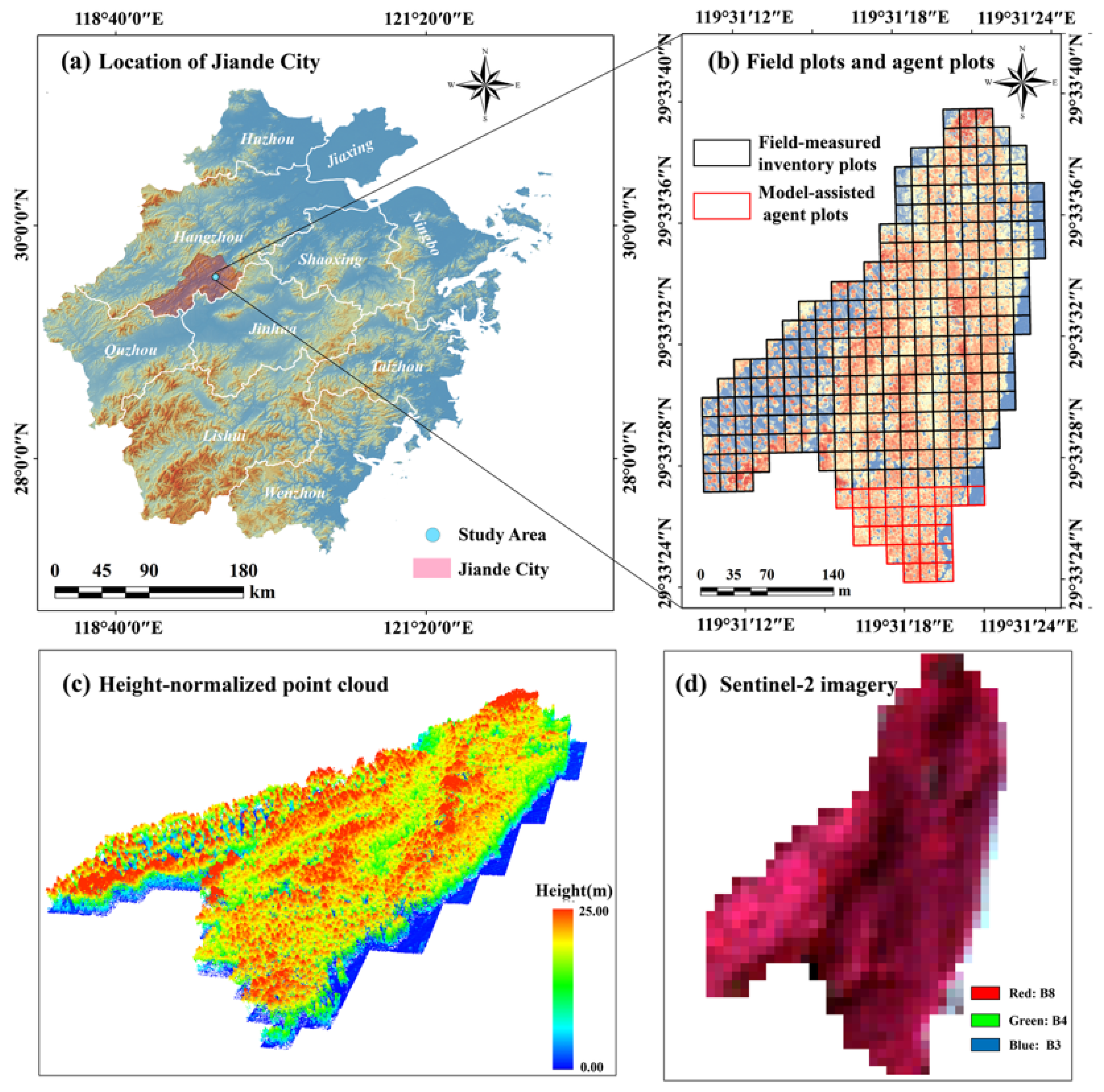
The study area is located in Jiande City (29°12′–29°46′N, 118°53′–119°45′E), Zhejiang Province, eastern China. The region lies in the upper reaches of the Qiantang River and has a subtropical monsoon climate characterized by warm and humid conditions, abundant precipitation, and distinct seasons. The mean annual temperature is 16.7 °C, with an average annual precipitation of approximately 1600 mm and about 1760 h of sunshine. Vegetation is dominated by subtropical evergreen broad-leaved forests, with a forest coverage of 76.2%. The principal plantation species include Chinese fir, Masson pine (Pinus massoniana), and Moso bamboo (Phyllostachys edulis), accompanied by deciduous broad-leaved species such as Chinese sweetgum (Liquidambar formosana) and oak species (Quercus spp.). As shown in Figure 1a, Jiande City is located in western Zhejiang Province, eastern China. Figure 1b shows the spatial distribution of the 28 field-measured inventory plots and the 263 model-assisted agent plots generated by spatially aggregating individual-tree AGB estimates. Figure 1c presents the height-normalized UAV-LiDAR point cloud, with colors representing height above ground, whereas Figure 1d shows the Sentinel-2 false-color composite using bands B8, B4, and B3, from which spectral predictors were derived for stand-level AGB modeling.

2.2. Data Acquisition

2.2.1. Acquisition of Chinese Fir AGB

Field surveys were conducted in August 2023 in Chinese fir plantations within Jiande Forest Farm. A total of 28 field plots, each measuring 20 m × 20 m, were established in the southern part of the study area. All Chinese fir trees within each plot were inventoried, resulting in a total of 447 measured trees. Descriptive statistics of diameter at breast height (DBH) and tree height for each field plot, including the mean, minimum, maximum, and variance, are provided in

Table A1. Plot-level statistics of DBH and tree height.

ID	DBH (cm)				Height (m)
	Mean	Maximum	Minimum	Variance	Mean	Maximum	Minimum	Variance
1	25.3	33.8	13.6	19.6	17.8	20.2	12.4	3.6
2	26.2	32.3	16.8	13.6	19.1	23.5	15.1	4.3
3	25.0	31.1	20.3	6.9	17.9	19.8	15.7	1.0
4	27.8	34.8	21.8	12.6	18.2	19.6	15.8	0.8
5	25.7	37.3	18.9	25.7	17.4	20.6	12.1	6.2
6	25.9	32.1	19.5	13.3	18.2	20.9	12.6	4.9
7	26.7	32.9	22.4	13.5	18.6	19.9	17.0	1.1
8	25.0	31.5	20.3	9.3	17.2	18.9	15.1	0.9
9	24.4	29.8	19.1	9.1	16.4	20.4	14.2	2.1
10	24.9	29.0	20.7	5.9	17.9	19.7	16.3	0.9
11	25.3	32.3	19.8	9.4	17.0	19.7	13.9	2.1
12	25.4	31.0	19.5	9.4	16.9	19.1	13.7	1.4
13	26.7	34.1	10.0	30.0	17.0	20.4	14.6	2.5
14	26.2	32.4	20.3	10.9	17.7	19.3	14.7	1.1
15	27.1	32.9	20.9	16.8	17.6	19.9	15.3	2.0
16	25.5	32.5	19.9	15.2	17.4	19.2	14.7	1.3
17	27.6	32.0	22.0	8.3	17.9	20.7	15.6	1.7
18	26.6	35.4	21.4	14.2	17.6	19.4	16.3	1.0
19	25.1	30.8	19.4	12.7	17.7	19.6	16.3	1.3
20	26.1	29.9	21.3	5.8	18.2	19.5	16.6	0.7
21	27.2	39.6	11.0	28.3	18.4	20.4	15.9	1.2
22	28.5	41.5	21.0	28.8	18.2	20.9	15.5	1.9
23	25.9	31.5	21.7	6.5	17.1	19.2	15.6	0.5
24	27.0	35.3	19.3	17.6	18.0	20.2	16.2	1.4
25	29.0	37.3	22.3	18.9	18.5	20.2	16.0	1.3
26	28.2	35.1	22.9	13.0	17.9	20.5	15.8	1.9
27	29.5	39.6	23.9	15.3	18.9	23.1	17.0	2.2
28	27.7	32.7	22.2	9.6	18.6	20.1	16.0	1.2

.

The position of each measured tree was recorded using a Huace i70II real-time kinematic global navigation satellite system (RTK-GNSS) receiver, with network corrections provided by a continuously operating reference station (CORS) service. The estimated horizontal and vertical positioning precisions reported by the receiver were ≤0.02 m and ≤0.03 m, respectively. DBH was measured at 1.3 m above the ground using a diameter tape. Tree height was calculated as the maximum height above ground within the height-normalized UAV-LiDAR point cloud of each segmented tree. This approach was adopted because Tao et al. [27] showed that UAV laser scanning provided more accurate individual-tree height estimates than ultrasonic altimeter measurements when evaluated against felled-tree reference heights in a Chinese fir plantation. The AGB of each Chinese fir tree was subsequently calculated using the following species-specific allometric model [28]:

$$W={0.086D}^{1.979}{H}^{0.419}$$

(1)

where $W$ is AGB (kg), $D$ is DBH (cm), and $H$ is tree height (m).

2.2.2. UAV-LiDAR Acquisition and Preprocessing

UAV-LiDAR data were acquired in July 2023 using a DJI Matrice 600 Pro UAV equipped with a Velodyne Puck LITE laser scanner. The scanner operated at a wavelength of 903 nm, with a maximum measurement range of 100 m, a ranging accuracy of ±3 cm, a vertical field of view of ±15°, a horizontal field of view of 360°, and a measurement rate of up to 300,000 pts/s. The survey produced high-density point-cloud data with an average density of approximately 200 pts/m².

The raw point clouds were first denoised using a statistical outlier removal filter. Ground points were then classified using the improved progressive triangulated irregular network (TIN) densification algorithm [29]. A digital elevation model (DEM) and a digital surface model (DSM) were generated through Kriging interpolation. Point-cloud heights were normalized by subtracting the corresponding DEM elevation from the elevation of each point, and the canopy height model (CHM) was derived from the difference between the DSM and DEM. Individual trees were segmented from the normalized point clouds using the seed-based individual-tree segmentation algorithm implemented in LiDAR360. Candidate treetops were identified from local maxima in the CHM and used as seed points for crown delineation [30].

The performance of individual-tree segmentation was evaluated using recall (R), precision (P), and the F1-score (F1). Recall measures the proportion of field-measured trees that were successfully detected, precision represents the proportion of segmented tree objects that were correctly matched, and the F1-score provides an overall assessment by balancing recall and precision. These metrics were calculated as follows:

$$\mathrm{R}={\displaystyle \frac{\mathrm{T}\mathrm{P}}{\mathrm{T}\mathrm{P}+\mathrm{F}\mathrm{N}}}\times 100\mathrm{\%}$$

(2)

$$\mathrm{P}={\displaystyle \frac{\mathrm{T}\mathrm{P}}{\mathrm{T}\mathrm{P}+\mathrm{F}\mathrm{P}}}\times 100\mathrm{\%}$$

(3)

$$\mathrm{F}1=2\times {\displaystyle \frac{\mathrm{R}\times \mathrm{P}}{\mathrm{R}+\mathrm{P}}}\times 100\mathrm{\%}$$

(4)

where $TP$ is the number of correctly matched trees, $FN$ is the number of field-measured trees that were not correctly detected, and $FP$ is the number of segmented tree objects without corresponding field-measured trees. The automatic individual-tree segmentation results and corresponding accuracy metrics are presented in

Table A2. Accuracy assessment of individual tree segmentation.

TP	FN	FP	R (%)	P (%)	F1 (%)
411	36	20	91.9	95.3	93.6

. After accuracy assessment, incorrectly segmented crowns were corrected before individual-tree parameter extraction and AGB modeling.

2.2.3. Simulation of Airborne LiDAR Data

ALS data were simulated using the LargE-Scale remote sensing data and image Simulation framework (LESS) [31,32]. The high-density UAV-LiDAR point clouds were first converted into three-dimensional forest scenes using cubic voxels with a side length of 0.2 m. Voxel size is a critical parameter in point-cloud-based scene reconstruction because it controls the level of canopy structural detail retained in the virtual scene as well as the associated computational requirements. Excessively large voxels may merge adjacent canopy elements, fill small within-crown gaps, enlarge crown envelopes, and consequently alter the propagation and interception of simulated laser pulses. The 0.2 m voxel size was selected based on the spatial detail of the source UAV-LiDAR data and previous evaluations of voxel-based forest representations. Qi et al. [33] tested voxel sizes of 0.3, 0.5, 1.0, and 2.0 m and showed that simulation accuracy was strongly affected by voxel resolution, with voxel sizes smaller than 0.5 m generally required for accurate radiative transfer simulations and a resolution of approximately 0.3 m required to obtain acceptable bidirectional reflectance factor accuracy. Similarly, Widlowski et al. [34] demonstrated that the radiometric bias introduced by crown abstraction generally increased with voxel size, whereas Li et al. [35] showed that high-resolution voxels more accurately approximated detailed three-dimensional forest structures, although at a higher computational cost. Therefore, the 0.2 m voxel size used in this study was considered an appropriate compromise between retaining fine-scale canopy gaps and vertical structural heterogeneity and maintaining a manageable computational demand for stand-scale simulations.

A virtual linear-scanning ALS sensor was configured with an altitude of 800 m, a beam divergence of 1.2 × 10⁻⁴ rad, and a near-infrared laser wavelength. The simulations were performed in multi-ray mode using Monte Carlo ray tracing. The energy within each laser pulse was represented by multiple sub-rays following a Gaussian spatial distribution, allowing the interactions of the laser beam with different canopy elements to be modeled. The returned energy was recorded as full-waveform signals and subsequently converted into discrete returns through Gaussian decomposition.

2.2.4. Sentinel-2 Data Acquisition and Preprocessing

Sentinel-2 Level-2A surface reflectance imagery acquired on 9 September 2023 was accessed and downloaded through the Google Earth Engine (GEE) platform. The selected image had an overall cloud cover of 3% and was acquired during the same growing season as the UAV-LiDAR survey conducted, thereby reducing inconsistencies associated with seasonal changes in canopy conditions. No cloud- or cloud-shadow-contaminated pixels occurred within the study area; therefore, no additional cloud or cloud-shadow masking was required.

The Sentinel-2 Multispectral Instrument provides 13 spectral bands at spatial resolutions of 10, 20, and 60 m. Ten spectral bands were used in this study, including the blue (B2), green (B3), red (B4), and near-infrared (B8) bands at 10 m resolution, as well as the red-edge bands (B5, B6, and B7), narrow near-infrared band (B8A), and shortwave-infrared bands (B11 and B12) at 20 m resolution. The 60 m bands were excluded because their spatial resolution was unsuitable for the 20 m × 20 m stand-level sampling units. The 10 m bands were resampled to 20 m using nearest-neighbor interpolation, whereas the original 20 m bands were retained at their native resolution. All selected bands were aligned to a common 20 m grid, clipped to the study area, and projected to the WGS 84/UTM zone 50N coordinate reference system to ensure spatial consistency with the UAV-LiDAR data and agent plots.

2.3. Feature Extraction and Selection

2.3.1. Individual-Tree LiDAR Feature Extraction

The extracted individual-tree LiDAR variables are summarized in

Table 1. Individual-tree LiDAR feature variables.

Feature Type	Feature Name	Feature Description
Canopy Structure	S	2D convex-hull canopy area
	CD	Mean canopy diameter
	V	3D convex-hull canopy volume
Height	H1/H5/H10/H20/H25/H30/H40/H50/H60/H70/ H75/H80/H90/H95/H99	Canopy-height percentiles
	Hiq	Hiq = H75 − H25
	AIH1/AIH5/AIH10/AIH20/AIH25/AIH30/ AIH40/AIH50/AIH60/AIH70/AIH75/AIH80/ AIH90/AIH95/AIH99	Cumulative height percentiles
	AIHiq	AIHiq = AIH75 − AIH25
	Hmax/Hmin/Hmean/Hmed/Hmadme	Maximum, minimum, mean, median, and median absolute deviation of point heights
	Hvar/Hstd/Hskew/Hkurt/Hcv/Hsq/Hcm/ Hcanopy/Hmad	Variance, standard deviation, skewness, kurtosis, coefficient of variation, second- and third-order power means, canopy undulation rate, and mean absolute deviation of point heights.
Density	D1/D2/D3/D4/D5/D6/D7/D8/D9/D10	Point fraction above each height quantile

. LiDAR-derived metrics describing crown geometry, vertical structure, and return distribution were extracted for individual-tree AGB estimation. Crown-geometry variables included crown diameter, projected crown area, and point-cloud-derived crown volume. These variables characterize the horizontal extent and three-dimensional spatial occupancy of individual crowns and have commonly been used as geometric proxies for tree size and AGB [11,36,37]. Crown volume integrates horizontal crown extent and vertical development and may therefore provide a more comprehensive representation of overall crown size than any single crown dimension. Height-related variables included height percentiles and summary statistics, including the mean, median, maximum, standard deviation, skewness, and coefficient of variation of point heights. These metrics characterize tree height, the vertical distribution of returns, and within-crown structural heterogeneity. Higher canopy-height percentiles are commonly associated with larger tree dimensions and higher AGB, whereas measures of height dispersion describe variation in the vertical distribution of crown returns [8,10]. Density metrics were calculated as the proportions of LiDAR returns above successive relative-height thresholds. These metrics describe the relative distribution of returns among the lower, middle, and upper portions of the crown. A higher proportion of upper-crown returns may indicate greater occupancy of the upper crown, whereas the distribution of returns across multiple height levels provides a proxy for vertical crown organization.

2.3.2. Stand-Level LiDAR Feature Extraction

For stand-level AGB modeling, LiDAR metrics were extracted independently from the LESS-simulated ALS point clouds at the 20 m × 20 m agent plot scale. For each plot, the point cloud was clipped using the plot boundary and normalized relative to the ground surface. Height-distribution, height-statistical, and point-density metrics were then calculated from all normalized canopy points within the plot to characterize overall canopy height, vertical variability, and the relative distribution of LiDAR returns along the canopy profile.

The stand-level height and density metrics were calculated using the same definitions and computational procedures as those applied at the individual-tree scale. The difference lay in the spatial extent of the input point clouds: individual-tree metrics were derived from the point cloud of each tree crown, whereas stand-level metrics were calculated from all canopy points within each 20 m × 20 m agent plot. Thus, although variables such as Hmed, Hskew, and D8 retained the same abbreviations and calculation methods at both scales, they represented canopy structural characteristics at different spatial supports. The stand-level metrics were calculated directly from plot-level canopy point clouds rather than by averaging or aggregating the corresponding individual-tree metrics.

In addition to the conventional height and density metrics, the three-dimensional voxel index (3DVI) and three-dimensional profile index (3DPI) were calculated to characterize canopy volumetric occupancy and the vertical distribution of canopy material, respectively [38]. These indices were used to characterize canopy volumetric occupancy and vertical structural heterogeneity, and their parameters were optimized in this study to better represent the structural characteristics of Chinese fir canopies.

For the calculation of 3DVI, the plot-level point cloud was divided into cubic voxels, and the index was calculated as:

$$3DVI={\displaystyle \frac{N_{occupied}}{N_{projected}}}$$

(5)

where ($N_{occupied}$) is the number of voxels containing at least one canopy return and ($N_{projected}$) is the number of horizontal grid cells within the canopy projection. Thus, 3DVI represents the mean number of vertically occupied voxels per horizontally projected canopy cell and quantifies the three-dimensional spatial occupancy of canopy returns within each plot. Because increases in tree dimensions and canopy development can increase three-dimensional canopy occupancy, 3DVI was evaluated as a structural proxy for stand-level AGB.

The 3DPI was calculated to describe the distribution of LiDAR returns along the vertical canopy profile while accounting for the progressive interception of laser pulses by overlying canopy layers. Each plot-level point cloud was divided into (n) vertical layers, and 3DPI was calculated as:

$$3DPI={\displaystyle \sum _{i=1}^n}\left[{\displaystyle \frac{p_i}{p_t}}exp\left(k{\displaystyle \frac{p_{cs,i}}{p_t}}\right)\right]$$

(6)

where $p_i$ is the number of canopy points within the vertical layer, $p_t$ is the total number of canopy points within the plot, and $p_{cs,i}$ is the cumulative number of points intercepted above the layer. The parameter $k$ is an attenuation-like correction coefficient that controls the weighting applied to layers located beneath different amounts of overlying canopy material, and $n$ is the number of vertical layers. Thus, 3DPI integrates the relative proportions of LiDAR returns across vertical canopy layers while accounting for the cumulative interception of laser pulses by the overlying canopy. It therefore provides a plot-level measure of the vertical organization and concentration of canopy returns. Because changes in stand AGB are commonly accompanied by changes in tree dimensions, crown development, canopy height, and vertical structural organization, 3DPI was evaluated in this study as a structural proxy for stand-level AGB.

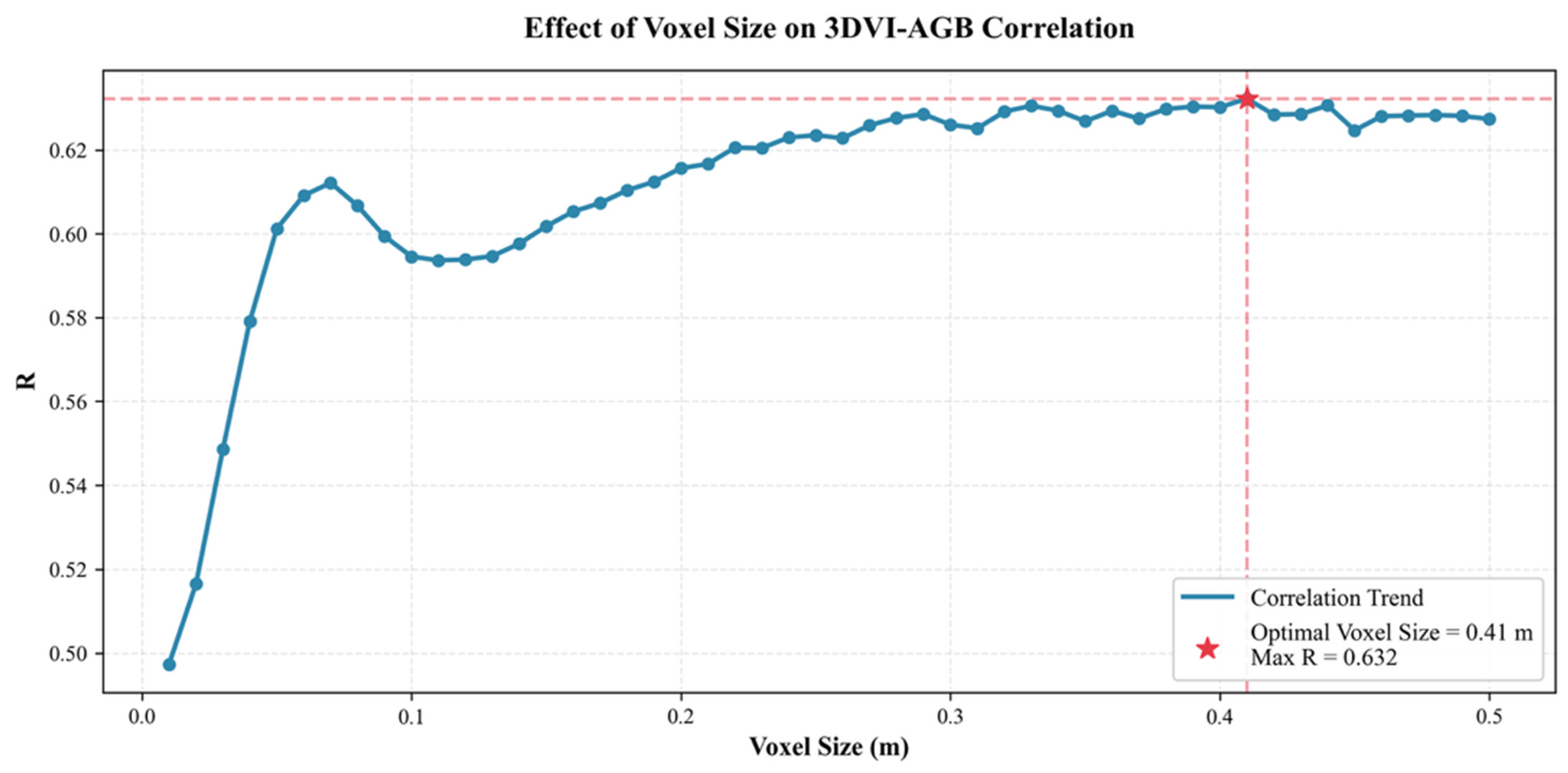
To identify parameter values appropriate for the canopy structure of Chinese fir plantations, a grid-search-based sensitivity analysis was conducted instead of directly adopting empirical values from previous studies. Parameter performance was assessed using the Pearson correlation coefficient between each derived structural index and the reference AGB. For 3DVI, the cubic voxel size was varied systematically from 0.01 to 0.50 m at intervals of 0.01 m. As shown in Figure A1 (Appendix B), the correlation between 3DVI and reference AGB reached its maximum at a voxel size of 0.41 m. This value was therefore selected for subsequent feature extraction.

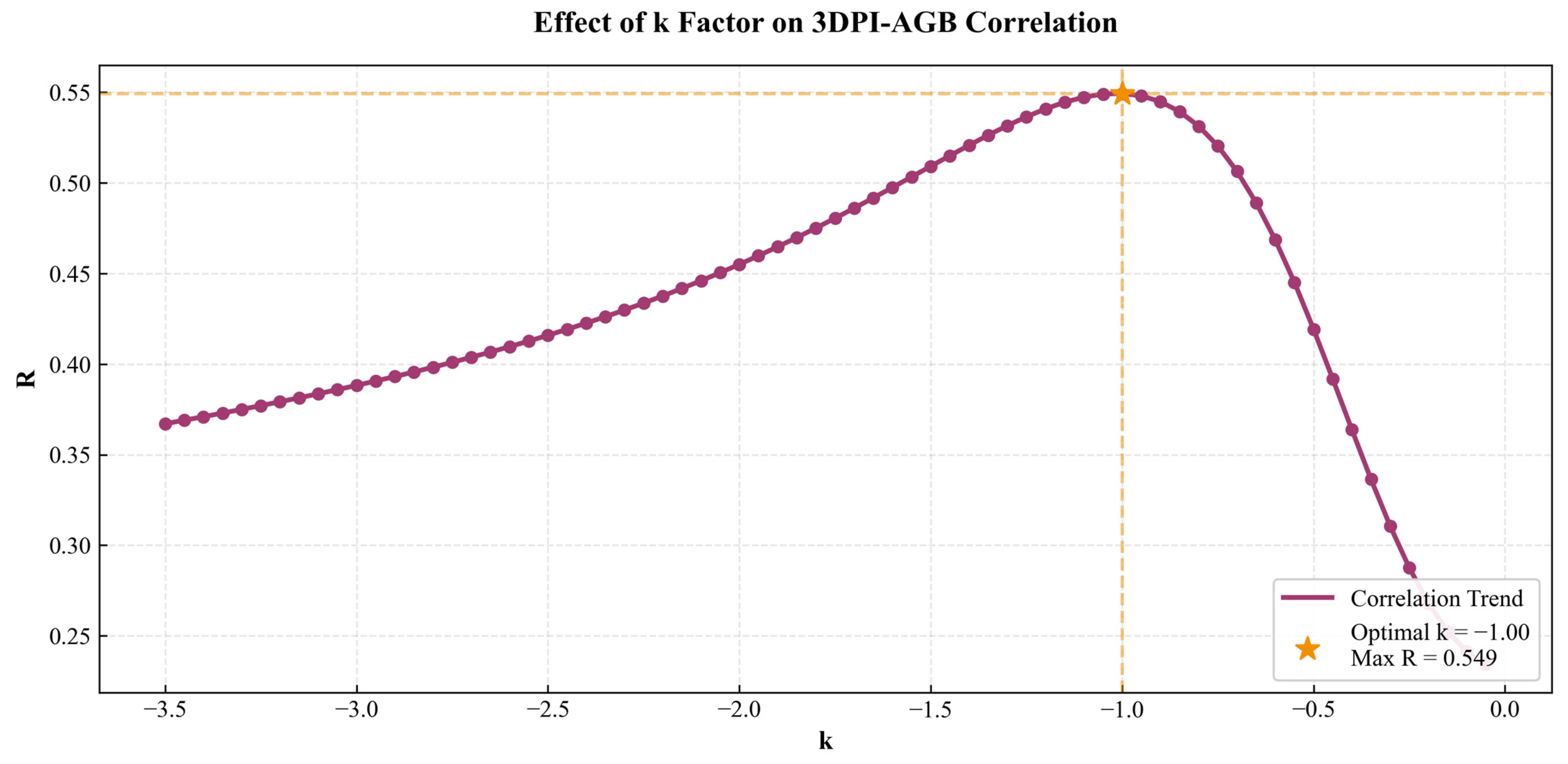
For 3DPI, the vertical layer thickness was fixed at 0.02 m. The parameter $n$ was not assigned a constant value but was determined separately for each agent plot according to the range between its minimum and maximum canopy heights. Accordingly, $n$ represents the plot-specific number of 0.02 m vertical intervals required to span the complete canopy profile. The parameter $k$ was searched from −3.50 to 0 at intervals of 0.05. Figure A2 (Appendix B) shows that the correlation between the 3DPI and reference AGB was maximized at $k$ = −1.00, which was subsequently used for all 3DPI calculations.

2.3.3. Sentinel-2 Feature Extraction

Sentinel-2 features were extracted from the preprocessed Level-2A surface reflectance imagery and comprised three categories: original spectral bands, spectral indices, and texture metrics. These variables were used to characterize canopy spectral reflectance, vegetation greenness, pigment and moisture conditions, and the spatial heterogeneity of forest canopies.

Ten original spectral bands were retained, including the visible bands B2–B4, red-edge bands B5–B7, near-infrared bands B8 and B8A, and shortwave-infrared bands B11 and B12. The 60 m atmospheric bands B1 and B9 were not included in the candidate feature dataset.

Twelve spectral indices were calculated from the selected bands: the Difference Vegetation Index (DVI), Enhanced Vegetation Index (EVI), Triangular Vegetation Index (TVI), Ratio Vegetation Index (RVI), Plant Senescence Reflectance Index (PSRI), Normalized Difference Infrared Index (NDII), Normalized Difference Water Index (NDWI), Normalized Difference Vegetation Index (NDVI), Modified Normalized Difference Water Index (MNDWI), Soil-Adjusted Vegetation Index (SAVI), Normalized Difference Built-up Index (NDBI), and red-edge Chlorophyll Index (CIre). These indices provided complementary information related to vegetation greenness, chlorophyll and senescence status, canopy moisture, and spectral variations associated with canopy and background conditions. Their equations, abbreviations, and references are provided in

Table 2. Sentinel-2 feature variables.

Type	Name	Calculation Models	Abbreviation	References
Original band	Blue	/	B2	/
	Green	/	B3	/
	Red	/	B4	/
	Red Edge 1	/	B5	/
	Red Edge 2	/	B6	/
	Red Edge 3	/	B7	/
	NIR	/	B8	/
	Red Edge 4	/	B8A	/
	SWIR 1	/	B11	/
	SWIR 2	/	B12	/
Spectral vegetation indices	DVI	$NIR-R$	DVI	[39]
	EVI	${\displaystyle \frac{\left(2.5\left(NIR-R\right)\right)}{\left(NIR+6R-7.5B+1\right)}}$	EVI	[40]
	TVI	$0.5\left(120\left(NIR-G\right)-200\left(R-G\right)\right)$	TVI	[41]
	RVI	${\displaystyle \frac{NIR}{R}}$	RVI	[42]
	PSRI	$\left(R-B\right)\times RedEdge2$	PSRI	[43]
	NDII	${\displaystyle \frac{\left(NIR-SWIR1\right)}{\left(NIR+SWIR1\right)}}$	NDII	[44]
	NDWI	${\displaystyle \frac{\left(G-NIR\right)}{\left(G+NIR\right)}}$	NDWI	[45]
	NDVI	${\displaystyle \frac{\left(NIR-R\right)}{\left(NIR+R\right)}}$	NDVI	[46]
	MNDWI	${\displaystyle \frac{\left(G-SWIR1\right)}{\left(G+SWIR1\right)}}$	MNDWI	[47]
	SAVI	$1.5\times {\displaystyle \frac{\left(NIR-R\right)}{\left(NIR+R+0.5\right)}}$	SAVI	[40]
	NDBI	${\displaystyle \frac{\left(SWIR1-NIR\right)}{\left(SWIR1+NIR\right)}}$	NDBI	[48]
	Cire	$\left(\left({\displaystyle \frac{RedEdge3}{RedEdge1}}\right)-1\right)$	Cire	[49]
Texture features based on the gray-level co-occurrence matrix (GLCM)	Variance	${\displaystyle \sum _{k=1}^n}{\displaystyle \sum _{l=1}^n}{\left(k-mean\right)}^2{P}_{kl}$	VAR	[50]
	Homogeneity	${\displaystyle \sum _{k=1}^n}{\displaystyle \sum _{l=1}^n}{\displaystyle \frac{1}{1+{\left(k-l\right)}^2}}{P}_{\left(k,l\right)}$	HOM	[50]
	Contrast	${\displaystyle \sum _{\left|k-l\right|=0}^{n-1}}{\left|k-l\right|}^2\left\{{\displaystyle \sum _{k=1}^n}{\displaystyle \sum _{l=1}^n}{P}_{\left(k,l\right)}\right\}$	CON	[50]
	Dissimilarity	${\displaystyle \sum _{\left|k-l\right|=0}^{n-1}}\left|k-l\right|\left\{{\displaystyle \sum _{k=1}^n}{\displaystyle \sum _{l=1}^n}{P}_{\left(k,l\right)}\right\}$	DIS	[51]
	Entropy	$-{\displaystyle \sum _{k=1}^n}{\displaystyle \sum _{l=1}^n}{P}_{\left(k,l\right)}\mathit{log}\left(P\left(k,l\right)\right)$	ENT	[50]
	Angular second moment	${\displaystyle \sum _{k=1}^n}{\displaystyle \sum _{l=1}^n}{P\left(k,l\right)}^2$	ASM	[50]
	Correlation	${\displaystyle \frac{{\displaystyle {\sum }_{k=1}^n}{\displaystyle {\sum }_{l=1}^n}kl{P_{\left(k,l\right)}}^2-{\mu }_x{\mu }_y}{{\sigma }_x{\sigma }_y}}$	COR	[50]
	Cluster shade	${\displaystyle \sum _{k=1}^n}{\displaystyle \sum _{l=1}^n}{\left(k+l-{\mu }_k-{\mu }_l\right)}^3{P}_{\left(k,l\right)}$	SHA	[51]

.

Texture features were derived using the gray-level co-occurrence matrix (GLCM) to characterize spatial variations in canopy reflectance that could not be represented by individual spectral values alone. The GLCM analysis was applied to six spectral bands—B2, B3, B4, B8, B11, and B12—covering the visible, near-infrared, and shortwave-infrared regions. Eight texture metrics were calculated: variance (VAR), homogeneity (HOM), contrast (CON), dissimilarity (DIS), entropy (ENT), angular second moment (ASM), correlation (COR), and cluster shade (SHA). Because GLCM texture metrics are sensitive to neighborhood size, moving windows of 3 × 3, 5 × 5, and 7 × 7 pixels were used. The multiscale windows were used to capture spatial variations in canopy reflectance from relatively local crown and gap patterns to broader stand-level configurations.

The combination of six spectral bands, eight GLCM metrics, and three window sizes generated 144 texture variables. Together with the 10 original spectral bands and 12 spectral indices, a total of 166 candidate Sentinel-2 variables were extracted.

2.3.4. Feature Selection

To reduce feature redundancy and retain variables relevant to AGB estimation, feature selection was performed using the BorutaShap algorithm [22]. BorutaShap extends the Boruta framework by evaluating feature importance using SHAP [20,52]. For each original predictor, a shadow feature was generated by randomly permuting its observed values. The importance of each original variable was then compared with the importance distribution of the shadow features over repeated iterations. Variables that consistently exhibited greater importance than the shadow-feature threshold were classified as confirmed and retained for subsequent modeling, whereas rejected variables were removed [52].

Feature selection was conducted separately for the individual-tree and stand-level datasets because the variables at the two scales represented different spatial supports. At the individual-tree scale, BorutaShap was applied to the 59 candidate LiDAR metrics extracted from individual-tree point clouds. At the stand level, each simulated ALS point-density dataset initially contained 58 LiDAR variables, comprising 46 height-distribution and statistical metrics, 10 density metrics, and the two three-dimensional structural indices, 3DVI and 3DPI. The Sentinel-2 dataset contained 166 candidate variables, including 10 original spectral bands, 12 spectral indices, and 144 GLCM texture variables. Consequently, each integrated ALS–Sentinel-2 dataset contained 224 candidate variables.

Because changes in point-cloud density may alter the stability and predictive relevance of LiDAR-derived metrics, BorutaShap was applied independently to the ALS datasets at 0.5, 1, 2, 5, and 10 points/m². Feature selection was also performed independently for the Sentinel-2-only dataset and for each of the five integrated ALS–Sentinel-2 datasets. Thus, no fixed feature subset derived from one density scenario was directly transferred to another density scenario.

To prevent information leakage during model validation, feature selection was fitted using only the training samples within each data split. The selected feature subset was subsequently applied without modification to the corresponding validation or test samples. All subsequent training and testing of the regression models were performed exclusively using the feature subsets selected by BorutaShap within the corresponding training split; variables not selected in that split were excluded from model fitting. Within a given data configuration and split, the same selected variables were used for support vector regression (SVR), RF, XGBoost, and TabPFN to ensure a consistent comparison among models.

2.4. AGB Modeling

2.4.1. Individual-Tree AGB Modeling

Individual-tree AGB models were developed using the 447 field-measured Chinese fir trees. The AGB of each tree was calculated using the allometric equation described in Section 2.2.1. Two types of modeling approaches were evaluated: feature-based tabular regression models using the LiDAR metrics described in Section 2.3.1 and an end-to-end deep learning model using the corresponding raw individual-tree point clouds. TabPFN is a pretrained foundation model for tabular prediction that operates through in-context learning. At inference, it conditions on the labeled training samples and predicts the unlabeled validation or test samples in a forward pass without iterative task-specific fitting. The target values of the validation or test samples were not provided to the model [19]. SVR estimates nonlinear regression functions using kernel-based learning within an ε-insensitive loss framework [53]. RF is an ensemble learning algorithm that combines multiple decision trees constructed through bootstrap sampling and random feature selection [54]. XGBoost employs a gradient boosting framework with regularization to improve model generalization and computational efficiency [55]. To ensure reliable model comparison, SVR and RF were implemented using scikit-learn (version 1.5.1), whereas XGBoost was implemented using XGBoost (version 3.0.2). The hyperparameters of SVR, RF, and XGBoost were optimized using Bayesian optimization implemented with the bayesian-optimization package (version 3.1.0). TabPFN was implemented using the tabpfn package (version 2.2.1) with its default pretrained configuration. The hyperparameter search spaces used for Bayesian optimization are summarized in

Table A3. Hyperparameter search spaces used for Bayesian optimization.

Model	Hyperparameter	Search Range
SVR	C	[0.01, 1000.0]
	gamma	[1 × 10−4, 1.0]
	epsilon	[0.01, 1.0]
	kernel	{‘rbf’, ‘linear’}
Random Forest	n_estimators	[50, 2000]
	max_depth	[3, 20]
	min_samples_split	[2, 10]
	min_samples_leaf	[1, 10]
XGBoost	n_estimators	[50, 2000]
	max_depth	[3, 15]
	learning_rate	[0.001, 0.3]
	subsample	[0.5, 1.0]
	colsample_bytree	[0.5, 1.0]

, and the optimal parameter combinations identified for SVR, RF, and XGBoost are reported in

Table A4. List of optimized hyperparameter values for each ML algorithm for all.

Dataset	SVR	RF	XGBoost
Individual-Tree	C = 281.42148746784335 epsilon = 1 gamma = 0.0221017 kernel = rbf	max_depth = 7 min_samples_leaf = 1 min_samples_split = 6 n_estimators = 1984	colsample_bytree = 1 learning_rate = 0.003236428 max_depth = 5 n_estimators = 2000 subsample = 0.5
0.5 pts/m2	C = 1000 epsilon = 0.01 gamma = 0.001069 kernel = rbf	max_depth = 10 min_samples_leaf = 1 min_samples_split = 4 n_estimators = 225	colsample_bytree = 1 learning_rate = 0.00532017 max_depth = 15 n_estimators = 872 subsample = 0.5
0.5 pts/m2 + Sentinel-2	C = 579.82150001 epsilon = 1 gamma = 0.00182439 kernel = rbf	max_depth = 20 min_samples_leaf = 1 min_samples_split = 3 n_estimators = 250	colsample_bytree = 1 learning_rate = 0.0028324 max_depth = 8 n_estimators = 1847 subsample = 0.5
1 pts/m2	C = 287.03827204 epsilon = 1 gamma = 0.01303958 kernel = rbf	max_depth = 13 min_samples_leaf = 1 min_samples_split = 2 n_estimators = 462	colsample_bytree = 0.90619799 learning_rate = 0.0026653 max_depth = 10 n_estimators = 1615 subsample = 0.76152616
1 pts/m2 + Sentinel-2	C = 203.68626191 epsilon = 1 gamma = 0.01010687 kernel = rbf	max_depth = 16 min_samples_leaf = 2 min_samples_split = 2 n_estimators = 2000	colsample_bytree = 0.5 learning_rate = 0.00514093 max_depth = 3 n_estimators = 2000 subsample = 0.5
2 pts/m2	C = 128.85137982 epsilon = 1 gamma = 0.01665133 kernel = rbf	max_depth = 20 min_samples_leaf = 3 min_samples_split = 2 n_estimators = 52	colsample_bytree = 0.90619799 learning_rate = 0.0026653 max_depth = 10 n_estimators = 1615 subsample = 0.76152616
2 pts/m2 + Sentinel-2	C = 225.47323048 epsilon = 1 gamma = 0.0047147 kernel = rbf	max_depth = 11 min_samples_leaf = 1 min_samples_split = 2 n_estimators = 50	colsample_bytree = 0.95619281 learning_rate = 0.00315064 max_depth = 10 n_estimators = 1896 subsample = 0.71473485
5 pts/m2	C = 106.1675971 epsilon = 0.01 gamma = 0.04601912 kernel = rbf	max_depth = 20 min_samples_leaf = 3 min_samples_split = 2 n_estimators = 52	colsample_bytree = 0.70744516 learning_rate = 0.01505705 max_depth = 15 n_estimators = 693 subsample = 0.5
5 pts/m2 + Sentinel-2	C = 145.70226221 epsilon = 0.01 gamma = 0.02577348 kernel = rbf	max_depth = 20 min_samples_leaf = 1 min_samples_split = 3 n_estimators = 1563	colsample_bytree = 0.94832004 learning_rate = 0.00399553 max_depth = 10 n_estimators = 2000 subsample = 0.5
10 pts/m2	C = 479.2874236 epsilon = 0.11890131 gamma = 0.00570773 kernel = rbf	max_depth = 11 min_samples_leaf = 1 min_samples_split = 2 n_estimators = 2000	colsample_bytree = 1 learning_rate = 0.00727664 max_depth = 15 n_estimators = 1741 subsample = 0.5
10 pts/m2 + Sentinel-2	C = 1000 epsilon = 0.01 gamma = 0.00181401 kernel = rbf	max_depth = 9 min_samples_leaf = 1 min_samples_split = 2 n_estimators = 2000	colsample_bytree = 1 learning_rate = 0.00731432 max_depth = 10 n_estimators = 1772 subsample = 0.56783153

(Appendix A).

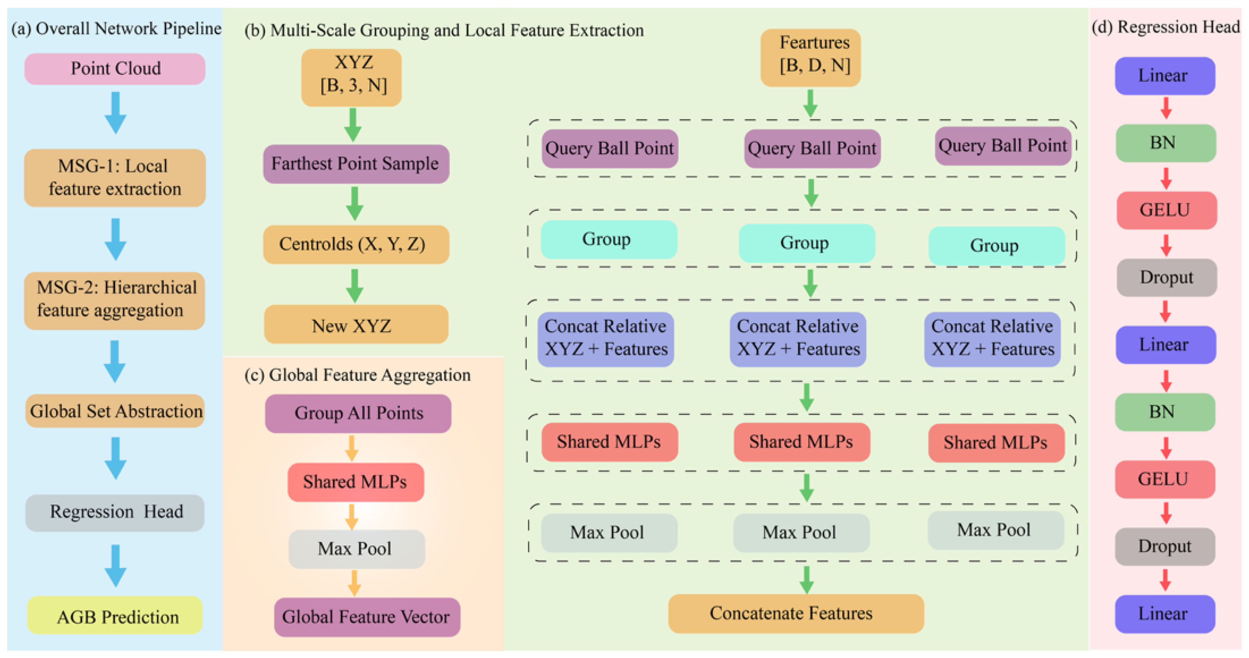
In parallel, PointNet++ was implemented to estimate individual-tree AGB directly from raw three-dimensional point clouds without relying on manually derived LiDAR metrics [56]. As shown in Figure 2, the model adopts set abstraction modules with multi-scale grouping (MSG) to accommodate complex tree structures and uneven point densities. Farthest point sampling (FPS), together with customized neighborhood radii, was used to hierarchically extract and integrate local geometric features. These features were subsequently aggregated by a global Set Abstraction layer into a 1024-dimensional global representation. A regression head composed of fully connected layers, Batch Normalization, and Dropout then transformed this representation into a single AGB estimate. To improve training stability and reduce the influence of extreme residuals, the model was trained using the Huber loss function, with the response variable transformed into logarithmic space.

2.4.2. Tree-to-Stand Upscaling and Agent Plot Generation

The optimal individual-tree AGB model identified in Section 2.4.1 was applied to the LiDAR-derived features of 3891 Chinese fir trees within the UAV-LiDAR coverage area. This procedure generated an AGB estimate in kilograms for each individual tree. To bridge the individual-tree and stand scales, the predicted tree-level AGB values were spatially aggregated within 20 m × 20 m units, consistent with the dimensions of the field plots and the spatial scale adopted for stand-level modeling.

A point-cloud volume-weighted method was used to account for trees whose crowns intersected the boundaries of an agent plot [37]. Trees whose point clouds were completely contained within a plot contributed their full predicted AGB, whereas trees located entirely outside the plot made no contribution. For trees whose point clouds crossed a plot boundary, the contribution of each tree was determined according to the proportion of its three-dimensional point-cloud volume located within the plot. The total and within-plot point-cloud volumes of each boundary tree were calculated using the stratified convex hull algorithm.

The weighted AGB contributions of all trees located within or intersecting an agent plot were summed to obtain the total AGB of that plot. The resulting value was then converted from kilograms to megagrams and standardized by the plot area of 0.04 ha to obtain AGB density in Mg·ha⁻¹. This procedure ensured that boundary-intersecting trees were proportionally allocated rather than being completely included or excluded from the plot-level reference value.

A total of 263 agent plots with corresponding model-derived AGB reference values were generated. These agent plots expanded the spatial coverage and sample size of the stand-level reference dataset and were subsequently matched with the LESS-simulated ALS structural metrics and Sentinel-2 variables for stand-level AGB modeling. Unlike the 28 field plots, the AGB values of the agent plots were not obtained from direct field measurements but were derived from individual-tree model predictions and spatial aggregation. Because the stand-level AGB labels were generated by aggregating individual-tree AGB predictions, they inevitably contained uncertainties inherited from the individual-tree modeling and upscaling processes. This uncertainty was propagated through the same spatial aggregation procedure and quantified using the Monte Carlo framework described in Section 2.5.2.

2.4.3. Stand-Level Multi-Source AGB Modeling

Stand-level AGB models were developed using the 263 agent plots generated through the tree-to-stand upscaling procedure described in Section 2.4.2. Predictor variables consisted of the stand-level structural metrics derived from LESS-simulated ALS data and the spectral and textural variables extracted from Sentinel-2 imagery.

To evaluate the effects of LiDAR point-cloud density and multi-source data integration, 11 predictor configurations were constructed. These included one Sentinel-2-only configuration, five ALS-only configurations corresponding to point densities of 0.5, 1, 2, 5, and 10 pts/m², and five integrated configurations in which the Sentinel-2 variables were coupled with the ALS variables at each point-density level. The Sentinel-2 feature set remained identical across all integrated configurations, whereas the LiDAR features were independently extracted and selected for each simulated point density. Feature selection for each data configuration was conducted using the procedure described in Section 2.3.4.

Four regression algorithms were evaluated for every predictor configuration: SVR, RF, XGBoost, and TabPFN. The same agent-plot samples, data partitions, and selected predictor sets were used across the four algorithms within each configuration to ensure that differences in predictive performance were attributable to the modeling methods rather than to inconsistent input data. The hyperparameters of SVR, RF, and XGBoost were optimized using Bayesian optimization based exclusively on the training data, and the parameter search ranges and optimal settings are provided in Table A4.

The effects of point-cloud density were assessed by comparing model performance among the five ALS-only configurations. The contribution of Sentinel-2 information was evaluated by comparing each ALS-only configuration with its corresponding ALS–Sentinel-2 configuration at the same point density.

2.4.4. SHAP-Based Model Interpretation

SHAP was used to interpret the optimal stand-level multi-source AGB model. SHAP is based on Shapley value theory from cooperative game theory and attributes a model prediction to the contributions of individual input variables. For a given sample, the predicted value is represented as the sum of a model baseline and the contribution of each predictor. The contribution assigned to a variable is determined from its average marginal effect across different combinations of input variables, thereby accounting for the joint presence of other predictors [20].

The sign and magnitude of a SHAP value provide complementary information about the role of a predictor. A positive SHAP value indicates that the variable increases the predicted AGB relative to the model baseline, whereas a negative value indicates a decreasing effect. The absolute SHAP value represents the strength of the contribution, with larger values indicating a greater influence on the model prediction. Because SHAP provides additive and consistent feature attributions, it is suitable for interpreting complex nonlinear models and comparing the relative roles of predictors measured in different units.

2.5. Model Accuracy Assessment

2.5.1. Model Validation Strategy

In this study, model performance was evaluated using a two-step validation strategy to ensure both baseline accuracy and robust spatial generalization. First, a standard random hold-out validation was conducted, where the dataset was randomly divided into a training set (70%) and a testing set (30%) for initial model development and baseline evaluation. Second, to rigorously evaluate the model’s predictive performance across different geographic regions and mitigate the overestimation of accuracy caused by spatial autocorrelation, a spatial block cross-validation strategy was implemented [57]. Traditional random splitting may result in spatially adjacent samples appearing simultaneously in both the training and testing sets, thereby inflating performance metrics. To address this, the sample plots were partitioned into 10 spatially contiguous blocks using the k-means clustering algorithm based on their geographic coordinates. A 10-fold spatial cross-validation was then performed. In each iteration, all plots within one spatial block were held out as an independent test set, while the plots in the remaining nine blocks were used for model training. This spatial partitioning strategy enforces strict spatial independence between the training and testing phases, providing a more objective assessment of the model’s spatial generalization capability across the landscape.

Model performance in both validation steps was quantified using two commonly applied metrics: the coefficient of determination (R²) and the root mean squared error (RMSE). A higher R² and a lower RMSE generally indicate better predictive performance. The two metrics were calculated as follows:

$$R^2=1-{\displaystyle \frac{{\displaystyle {\sum }_{i=1}^n}{\left({\widehat{x}}_i-x_i\right)}^2}{{\displaystyle {\sum }_{i=1}^n}{\left(x_i-\overline{x}\right)}^2}}$$

(7)

$$RMSE=\sqrt{{\displaystyle \frac{1}{n}}{\displaystyle \sum _{i=1}^n}{\left(x_i-{\widehat{x}}_i\right)}^2}$$

(8)

where $n$ is the number of samples; $x_i$, $\overline{x}$, and ${\widehat{x}}_i$ represent the observed value, the mean of observations, and the predicted value, respectively.

2.5.2. Uncertainty Propagation and Nested Monte Carlo Validation

Because the stand-level AGB labels were generated by aggregating model-derived individual-tree AGB estimates, prediction errors from the individual-tree model were inevitably propagated to the agent-plot scale. Here, individual-tree AGB predictions refer to the model-derived AGB estimates generated by the individual-tree model selected based on validation performance. A two-stage Monte Carlo framework was therefore implemented to quantify the resulting uncertainty in the stand-level AGB labels and evaluate the robustness of the stand-level model under label perturbations.

First, the residuals of the optimal individual-tree AGB model were represented by a zero-mean homoscedastic normal distribution, with the standard deviation set equal to the RMSE obtained from the independent test dataset. For each agent plot, 1000 independent Monte Carlo iterations were conducted. In each iteration, a random residual was generated for every tree and added to its predicted AGB. The perturbed individual-tree AGB estimates were then aggregated using the same point-cloud volume-weighted procedure described in Section 2.4.2.

This procedure produced an empirical distribution of 1000 possible AGB values for each agent plot. The mean of the simulated values was used to characterize the central estimate of plot-level AGB, whereas the standard deviation was used to quantify the uncertainty propagated from individual-tree prediction to the stand scale.

A nested Monte Carlo validation procedure was subsequently used to examine the sensitivity of the optimal stand-level model to uncertainty in the response labels. The outer Monte Carlo layer consisted of 100 iterations. In each iteration, one AGB value was randomly sampled from the 1000 simulated values of every agent plot, thereby generating one realization of the stand-level response dataset. Within each realization, the optimal stand-level model was evaluated using fivefold cross-validation.

2.5.3. Stability Assessment of Feature Contributions

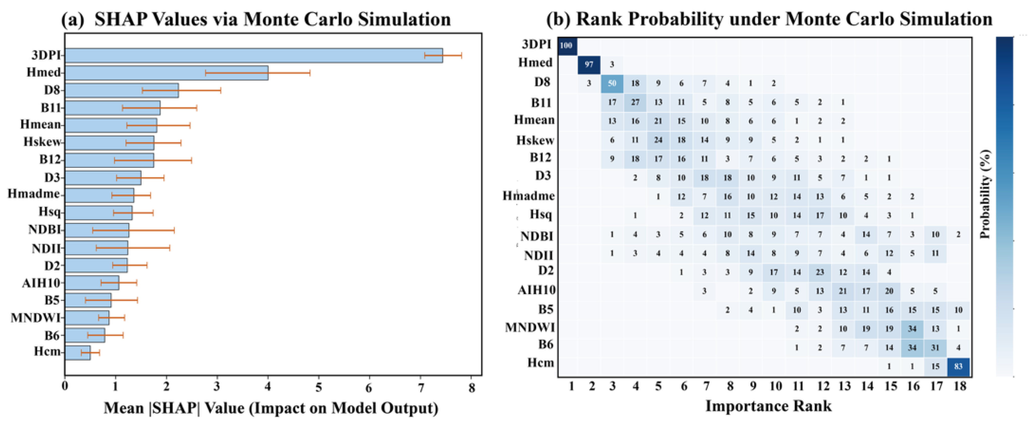
Because the stand-level AGB labels were derived from individual-tree predictions, uncertainty in these labels could affect the interpretation of feature contributions. A repeated Monte Carlo–SHAP framework was therefore used to assess whether the importance of the predictors remained stable under perturbations of the agent-plot AGB labels. The 100 Monte Carlo realizations of stand-level AGB labels generated in Section 2.5.2 were used in this analysis. For each realization, the optimal stand-level TabPFN modeling procedure and the corresponding SHAP analysis were repeated using the same predictor set and model configuration.

For each predictor, the mean absolute SHAP value across all agent plots was calculated within each Monte Carlo iteration to represent its global contribution to stand-level AGB estimation. The contribution magnitude of each variable was then summarized using the mean and 95% confidence interval of its mean absolute SHAP values across the 100 iterations. A narrow confidence interval indicated that the estimated contribution was relatively insensitive to perturbations in the AGB labels, whereas a wider interval indicated greater variability in model interpretation. Predictors were also ranked according to their mean absolute SHAP values in each iteration. The frequency with which a variable occupied each rank position across the 100 iterations was used to characterize its ranking probability. Variables that consistently occupied the highest ranks were considered to have robust contributions to AGB estimation, whereas variables with widely distributed rank positions were considered more sensitive to uncertainty in the response labels.

2.6. Overall Workflow

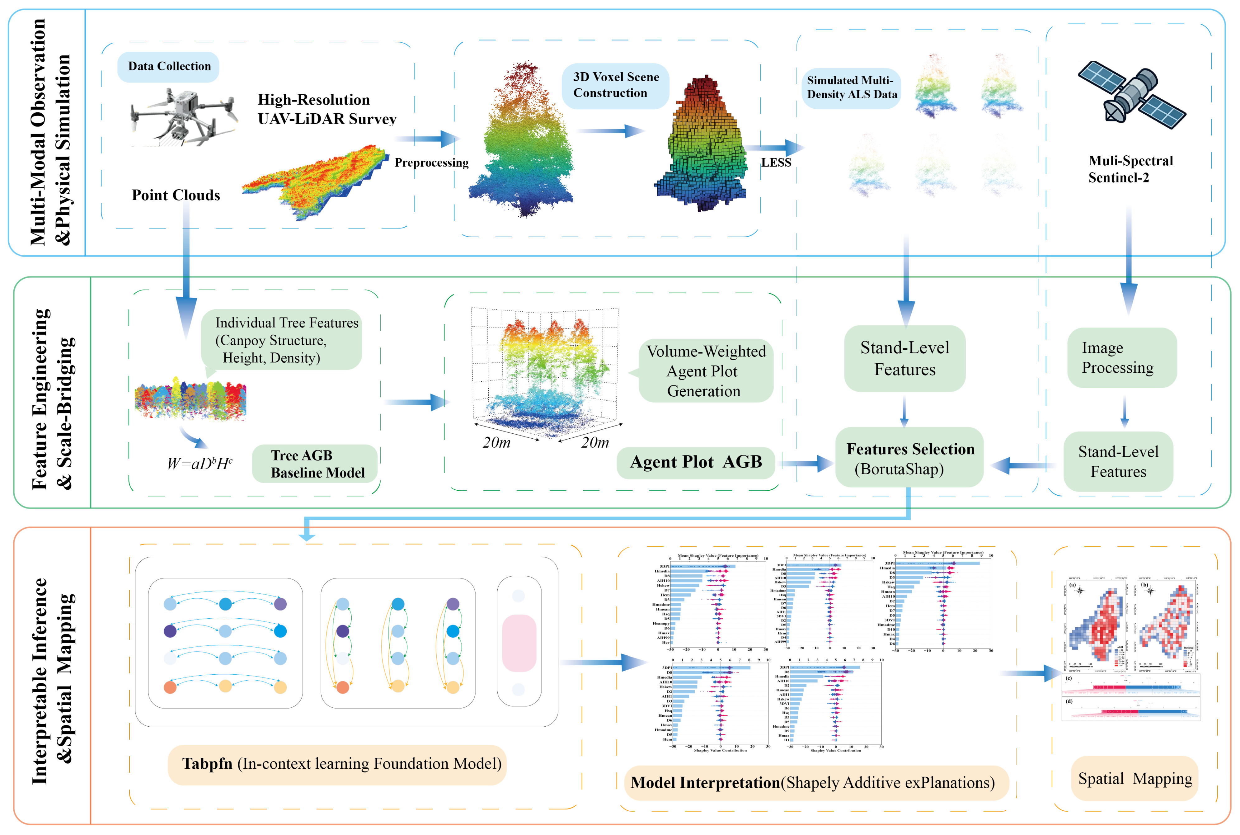
The overall workflow of this study is presented in Figure 3 and consists of three main stages. First, field measurements and high-density UAV-LiDAR data were used to develop individual-tree AGB models. The optimal tree-level model was then applied to the UAV-LiDAR-segmented Chinese fir trees, and the predicted AGB values were spatially aggregated using a canopy volume-weighted method to generate stand-level agent plots and their corresponding AGB reference values. Second, the UAV-LiDAR point clouds were used to construct three-dimensional forest scenes in the LESS model, from which ALS point clouds at multiple point densities were generated. LiDAR-derived canopy and vertical structural metrics were subsequently coupled with spectral, vegetation-index, and texture features extracted from Sentinel-2 imagery to develop multi-source machine learning models for stand-level AGB estimation and spatial mapping. Third, Monte Carlo simulations were used to propagate individual-tree prediction errors through the tree-to-stand aggregation process. Nested cross-validation based on the simulated AGB labels was then conducted to evaluate model robustness, while probabilistic SHAP analysis was used to assess the uncertainty and ranking stability of structural and spectral feature contributions.

3. Results

3.1. Evaluation of LESS-Simulated Airborne LiDAR

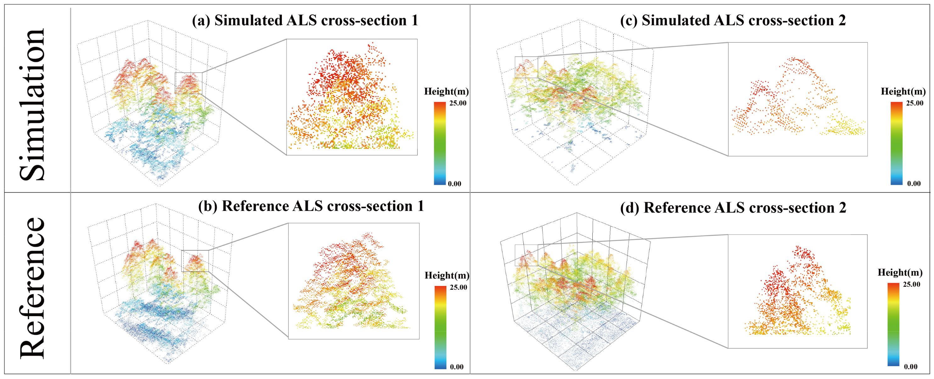
Figure 4 compares the cross-sectional profiles of the ALS data simulated with the LESS 3D radiative transfer model (ALS_sim) and the downsampled UAV-LiDAR data used as the reference (ALS_ref). Visually, the simulated point cloud successfully functions as a structural digital twin (Figure 4). However, at finer scales within the canopy, subtle structural shifts attributable to the inherent point aggregation effects of the voxelization process can be observed. While the reference data (ALS_ref) were characterized by highly textured and discrete point clusters, faithfully representing complex natural foliage clumping, the simulated data (ALS_sim) exhibited a physically based homogenized spatial point distribution within each voxel volume. This localized simplification is physically consistent, representing the necessary compromise when aggregating continuous fine-scale heterogeneities into discrete, managed voxel grids.

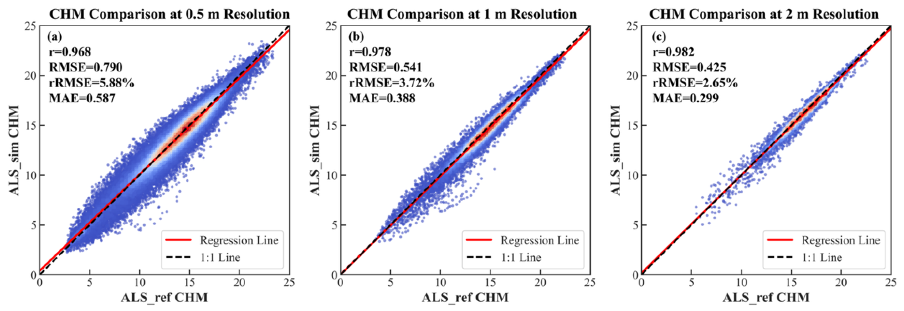
To further assess the accuracy of ALS_sim, we compared the CHMs, height-related metrics, and canopy density variables derived from ALS_sim with those obtained from ALS_ref. As shown in Figure 5, the simulated CHMs exhibited a very high level of agreement with the reference CHMs across all spatial resolutions. The correlation coefficients reached 0.9682 (0.5 m), 0.9788 (1 m), and 0.9821 (2 m). The slight higher correlation at coarser resolutions likely results from the smoothing of fine-scale canopy gaps and edge effects.

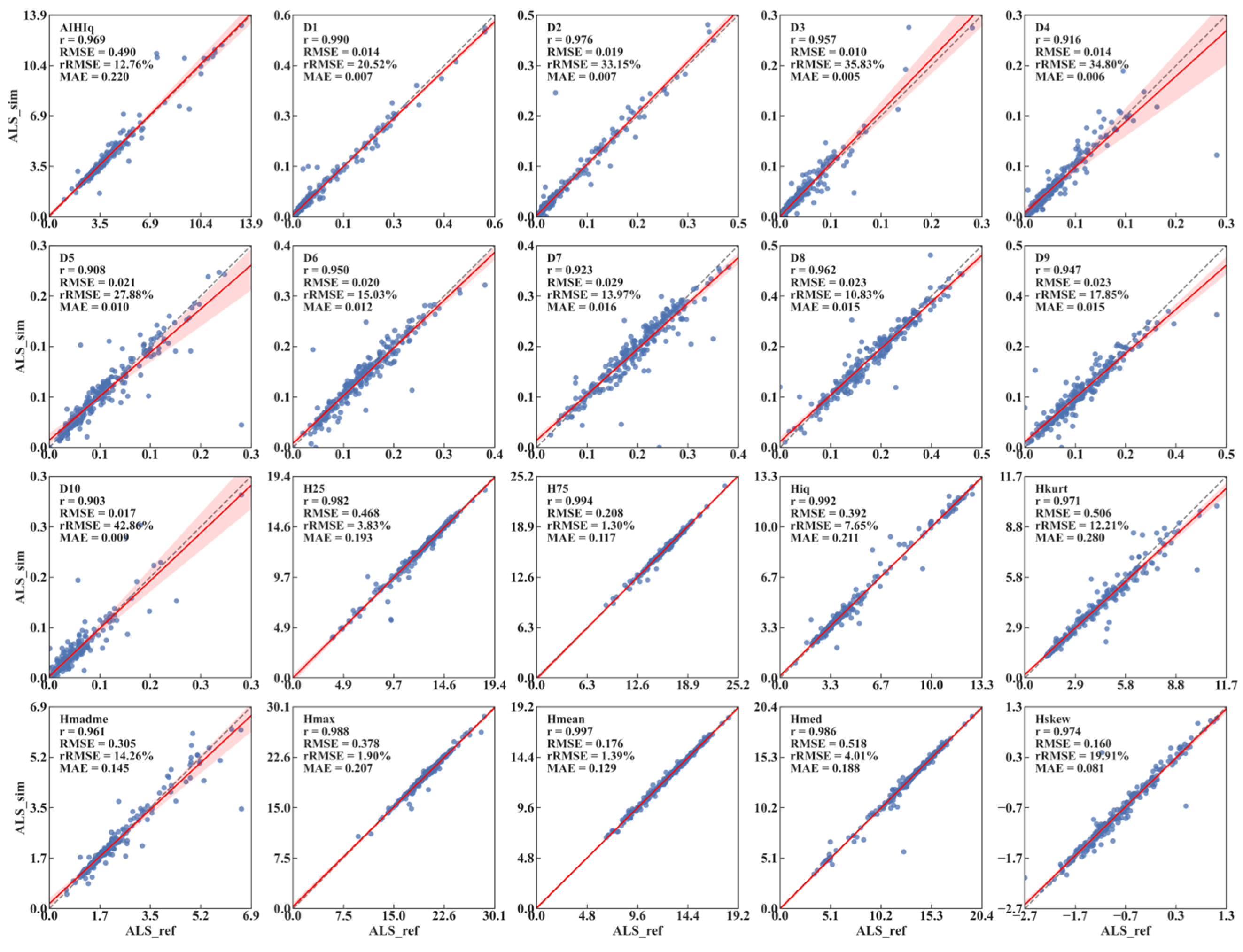
Height-derived metrics also demonstrated strong concordance (Figure 6), with Hmean and Hiq yielding correlations of 0.997 and 0.992, respectively, indicating high fidelity of vertical canopy structure. Canopy density metrics along the vertical axis generally showed correlations above 0.90, with a moderate decrease in upper-canopy density metrics (e.g., D10, r = 0.903), consistent with the reduced fine-scale detail in ALS_sim.

3.2. Multi-Density LiDAR Feature Stability Analysis

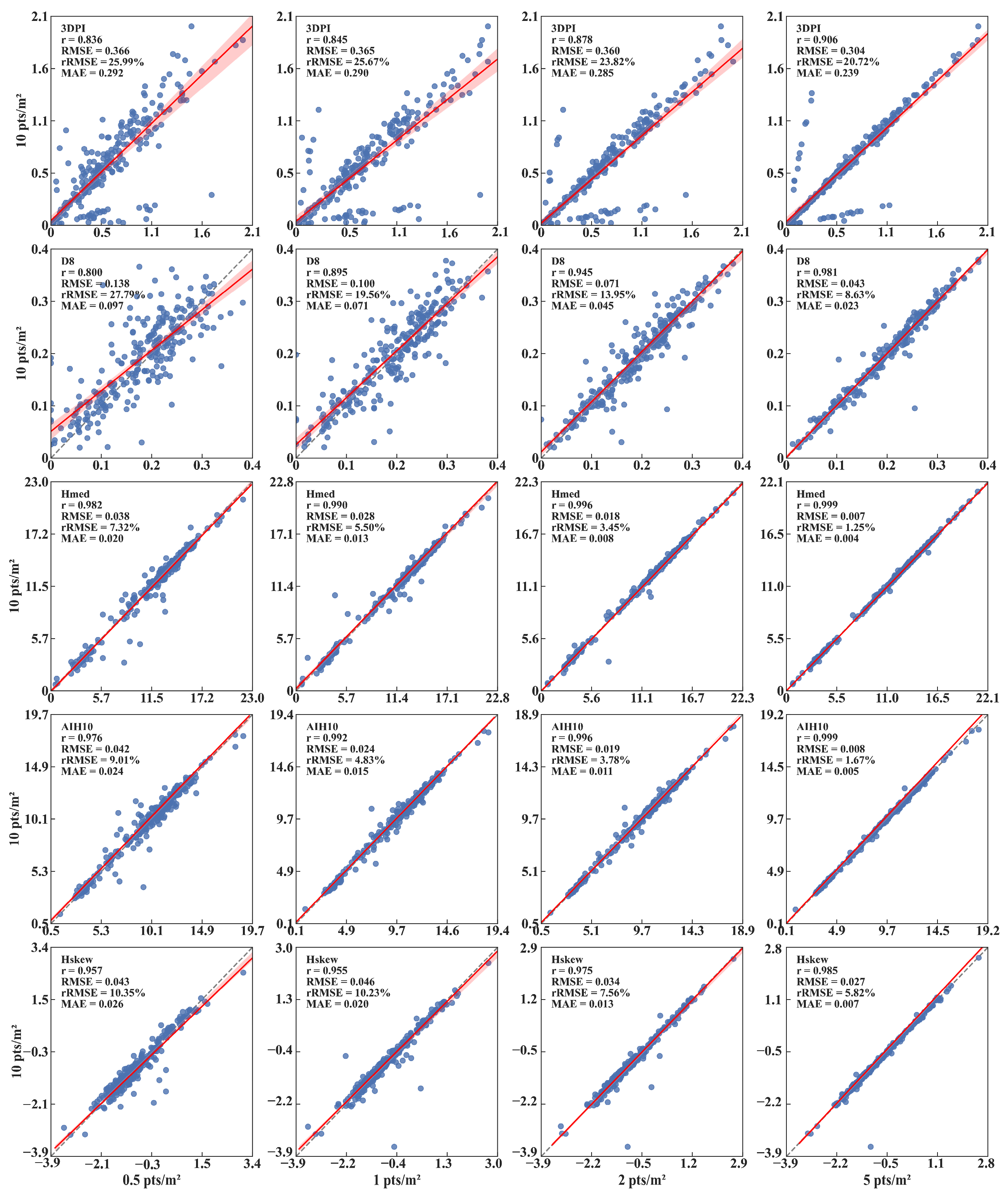
To assess the effect of simulated ALS point-cloud density on the stability of AGB-related features, four key variables (3DPI, Hmed, D8, and Hskew) were analyzed (Figure 7). Comparisons between low-density simulations (0.5–5 pts/m²) and the 10 pts/m² reference showed that feature stability increased with point-cloud density.

Height-based metrics (Hmed and Hskew) exhibited high robustness, with correlation coefficients consistently close to 1.0 across all densities, indicating that macro-scale canopy height characteristics are largely insensitive to point-cloud thinning.

In contrast, metrics describing internal canopy point distributions (3DPI and D8) were more sensitive to density reduction. At 0.5 pts/m², correlations with the reference decreased to 0.836 (3DPI) and 0.800 (D8). This sensitivity reflects their computational dependence on sufficient point sampling, as D8 relies on upper canopy point proportions, while 3DPI amplifies density fluctuations through weighted vertical aggregation.

3.3. AGB Estimation Accuracy Comparison

3.3.1. Individual-Tree AGB Estimation Using High-Density UAV-LiDAR

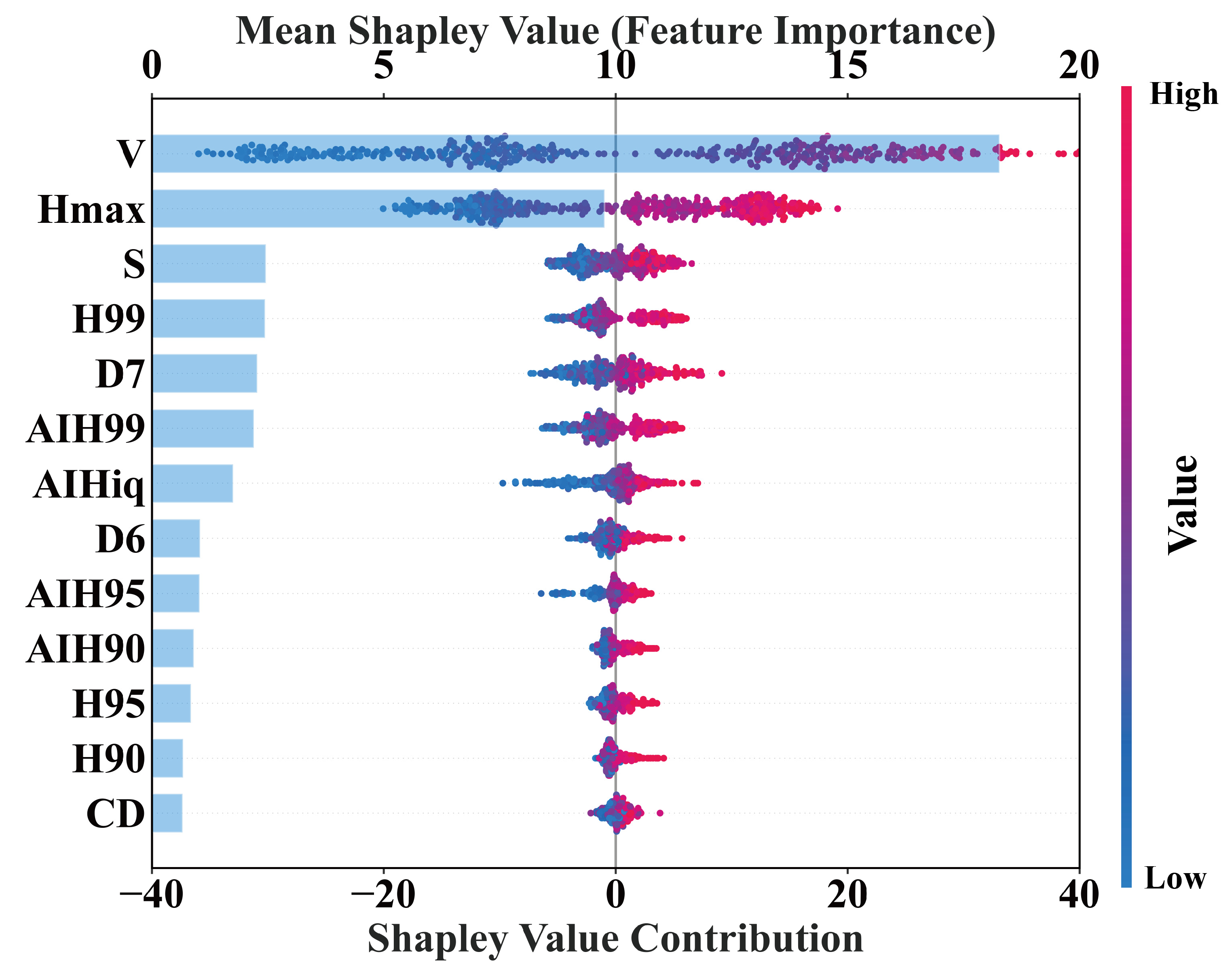
BorutaShap was applied to the complete set of candidate individual-tree LiDAR metrics and retained 13 predictors: V, Hmax, S, H99, D7, AIH99, AIHiq, D6, AIH95, AIH90, H95, H90, and CD (Figure 8). Only these selected predictors were used as inputs to SVR, RF, XGBoost, and TabPFN. V showed the highest mean absolute SHAP value, followed by Hmax, whereas S, H99, D7, and AIH99 exhibited moderate importance. The remaining retained variables made smaller contributions. For V and Hmax, high feature values were generally associated with positive SHAP contributions, while low values were predominantly associated with negative contributions.

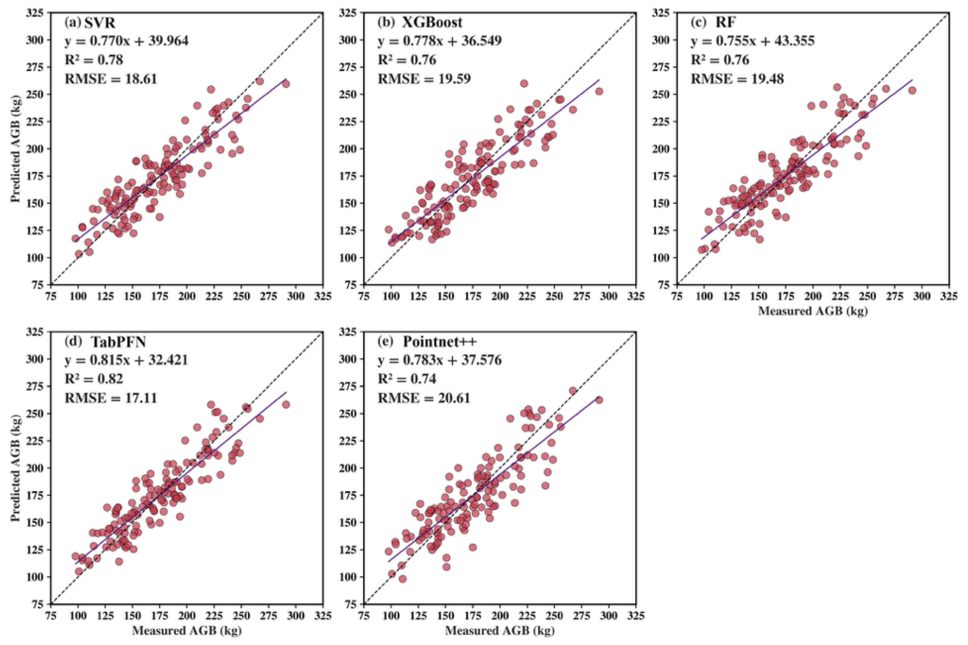
Figure 9 shows the estimation performance of different models for individual-tree AGB. Among the traditional machine learning approaches, SVR and RF exhibited similar predictive capability, both achieving an R² of 0.76, with RMSE values of 19.59 kg and 19.48 kg, respectively. XGBoost further improved the estimation accuracy, increasing the R² to 0.78 and reducing the RMSE to 18.61 kg, indicating the advantage of gradient boosting in capturing nonlinear relationships between LiDAR structural features and biomass. In contrast, TabPFN achieved the best overall performance, with the highest R² (0.82) and the lowest RMSE (17.11 kg), making it the only model surpassing the 0.80 threshold. Compared with XGBoost, TabPFN improved the R² by 0.04 and reduced the RMSE by 1.50 kg, while relative to SVR, the R² increased by 0.06 and RMSE decreased by 2.48 kg. These results demonstrate the strong robustness of TabPFN under limited-sample conditions, benefiting from its pre-trained prior knowledge and in-context learning mechanism.

The deep learning model PointNet++ directly utilized raw 3D point clouds for AGB estimation and achieved an R² of 0.74 with an RMSE of 20.61 kg. Although PointNet++ successfully captured the geometric structure of individual trees without handcrafted feature extraction, its performance was slightly lower than that of the feature-based machine learning models. One possible reason is that deep learning methods generally require large-scale training datasets to fully learn complex spatial patterns and avoid overfitting, whereas this study only included 447 individual-tree samples. Under such small-sample conditions, the advantages of deep neural networks in feature representation may not be fully realized. In addition, the structural heterogeneity and irregular point distribution within subtropical plantation canopies may further increase the difficulty of stable deep feature learning. In contrast, models such as TabPFN and XGBoost can more effectively leverage explicitly extracted LiDAR structural metrics under limited training data, resulting in superior estimation accuracy.

Using the optimal TabPFN model, individual-tree AGB was estimated for all 3891 trees segmented from the UAV-LiDAR point clouds. To upscale these predictions to the stand level, individual-tree AGB values were aggregated to the plot scale using a LiDAR point-cloud volume-weighted approach, which accounts for the proportional contribution of trees intersecting plot boundaries. This procedure ultimately generated 263 structurally reliable agent plot AGB samples, providing an expanded reference dataset for subsequent stand-level modeling and scale-bridging analysis.

3.3.2. Stand-Level AGB Feature Selection Using Simulated ALS and Sentinel-2

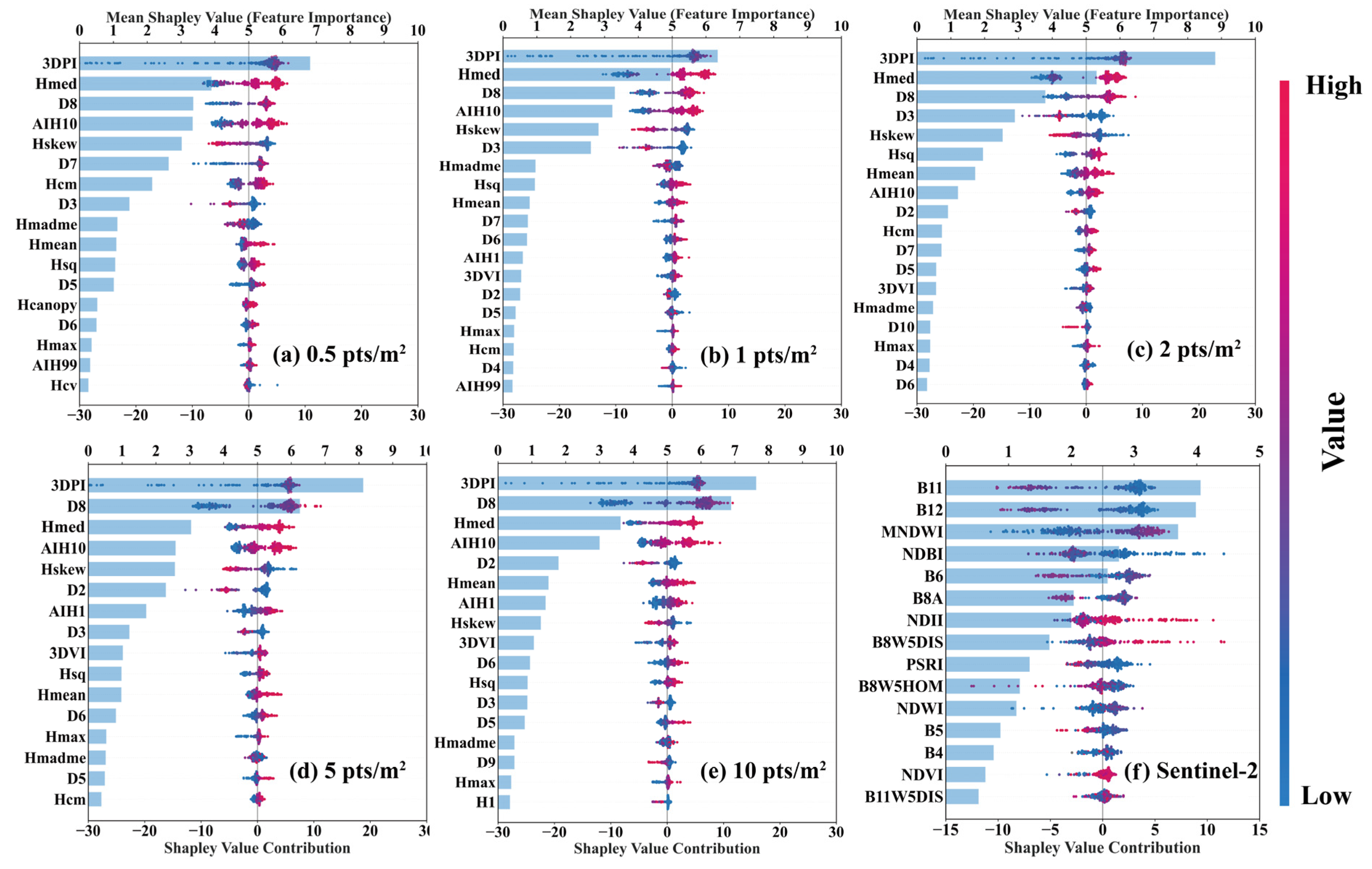
To assess the contribution of multi-source predictors to plot-level AGB estimation, BorutaShap feature selection was conducted separately for the five simulated ALS datasets with different point densities and for the Sentinel-2 dataset (Figure 10). The complete candidate feature set for each data configuration was first submitted to BorutaShap, and only the retained feature subset was used in the subsequent SVR, RF, XGBoost, and TabPFN models. Within each configuration, all four models were trained using the same selected predictors to ensure a consistent comparison of model performance.

The feature-selection results showed that LiDAR-derived structural metrics were consistently retained across densities (Figure 10). From 58 candidate ALS variables, BorutaShap retained 17, 19, 18, 16, and 17 features at 0.5, 1, 2, 5, and 10 pts/m², respectively. Among them, 3DPI generally ranked highest, followed by Hmed and D8. D8 importance decreased under sparse point-cloud conditions, whereas height-related metrics including Hmed remained relatively stable. For the Sentinel-2-only configuration, 15 out of 166 candidate variables were retained, dominated by SWIR bands B11 and B12, followed by MNDWI, NDBI, and red-edge band B6.

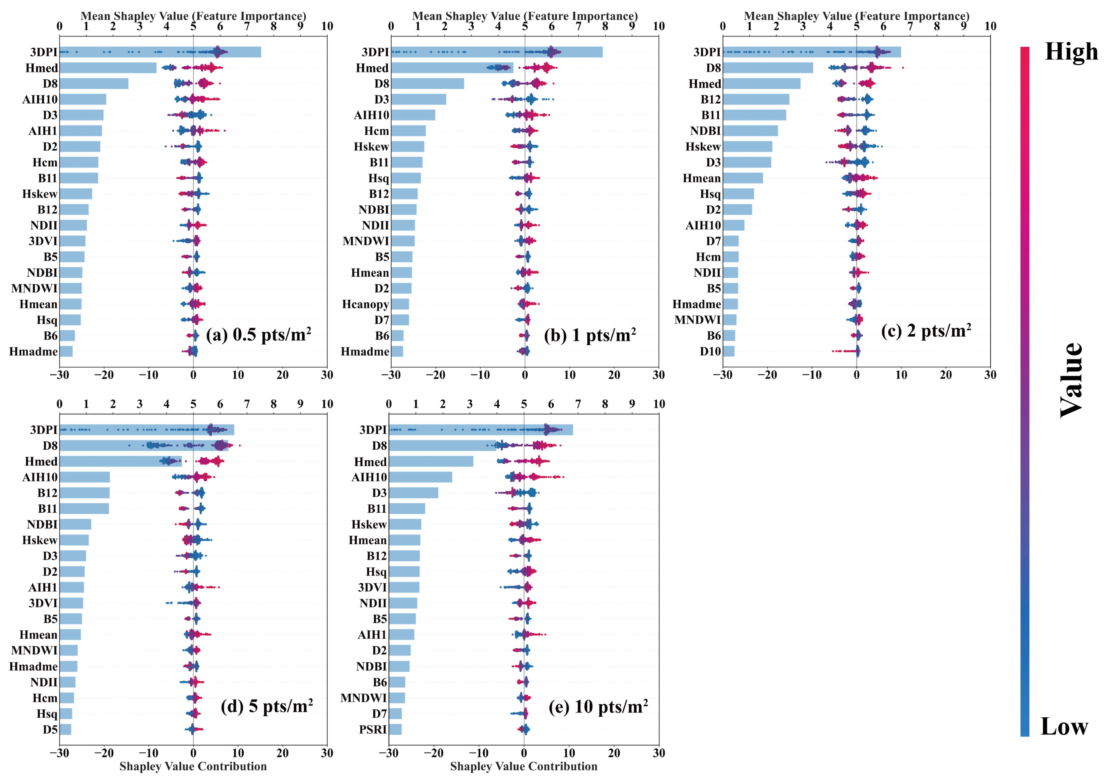
BorutaShap was also applied independently to each integrated ALS–Sentinel-2 configuration (Figure 11). Consequently, each point-density scenario produced its own screened multi-source feature subset, and only the predictors retained for that scenario were entered into the subsequent AGB models. LiDAR structural variables, particularly 3DPI, Hmed, and D8, generally occupied the highest importance ranks across the integrated configurations. Sentinel-2 variables, including B11 and B12, were repeatedly retained as additional predictors, although their relative rankings varied among point-density scenarios.

3.3.3. Stand-Level AGB Estimation Using Simulated ALS and Sentinel-2

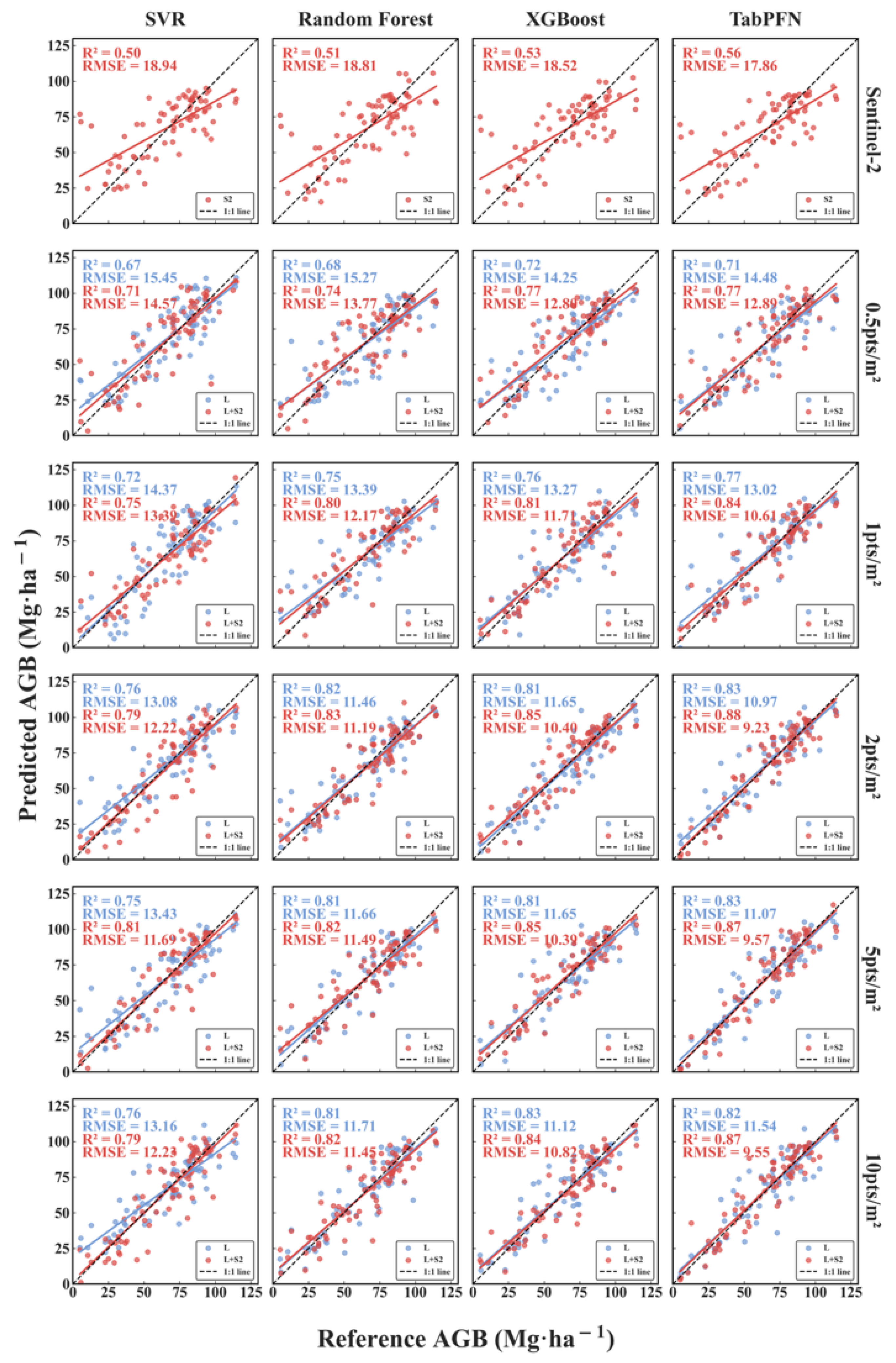
Figure 12 compares the performance of four machine learning models (SVR, RF, XGBoost, and TabPFN) for stand-level AGB estimation using Sentinel-2 data alone and under different LiDAR point densities and data combinations, with the corresponding accuracy metrics summarized in

Table 3. Accuracy comparison of models.

Feature Type	SVR		Random Forest		XGBoost		TabPFN
	R2	RMSE	R2	RMSE	R2	RMSE	R2	RMSE
Sentinel-2	0.50	18.94	0.51	18.81	0.53	18.52	0.56	17.86
0.5 pts/m2	0.67	15.45	0.68	15.27	0.72	14.25	0.71	14.48
1 pts/m2	0.72	14.37	0.75	13.39	0.76	13.27	0.77	13.02
2 pts/m2	0.76	13.08	0.82	11.42	0.81	11.65	0.83	10.97
5 pts/m2	0.75	14.43	0.81	11.66	0.81	11.65	0.83	11.07
10 pts/m2	0.76	13.16	0.81	11.71	0.83	11.12	0.82	11.54
0.5 pts/m2 + Sentinel-2	0.71	14.57	0.74	13.77	0.77	12.80	0.77	12.89
1 pts/m2 + Sentinel-2	0.75	13.62	0.80	12.17	0.81	11.71	0.84	10.61
2 pts/m2 + Sentinel-2	0.79	12.22	0.83	11.19	0.85	10.40	0.88	9.23
5 pts/m2 + Sentinel-2	0.81	11.69	0.82	11.49	0.85	10.85	0.87	9.57
10 pts/m2 + Sentinel-2	0.79	12.23	0.82	11.45	0.84	10.82	0.87	9.55

. When only Sentinel-2 spectral features were used, clear differences in predictive performance were observed. SVR and RF yielded the lowest accuracy (R² = 0.50 and 0.51, respectively), while XGBoost achieved a slightly higher R² of 0.53. TabPFN outperformed the other models, achieving the highest R² (0.56) and the lowest RMSE (17.86 Mg·ha⁻¹), highlighting its superior ability to model complex nonlinear-spectral AGB relationships.

When LiDAR information was incorporated, model performance improved markedly as point density increased. As LiDAR density rose from 0.5 to 2 pts/m², the accuracy of all models increased and gradually reached a stable level beyond 2 pts/m², indicating limited benefits from further density increases. TabPFN consistently achieved the highest accuracy across most density levels, with the R² increasing from 0.71 at 0.5 pts/m² to 0.83 at 2 pts/m² and showing no additional improvement at 5 or 10 pts/m². The remaining models showed similar trends, although their performance remained below that of TabPFN.

The integration of Sentinel-2 physiological features with LiDAR structural metrics revealed a strong synergistic compensation mechanism, particularly under sparse observation conditions. For instance, at the extreme low density of 0.5 pts/m², the inclusion of Sentinel-2 information (e.g., SWIR and water indices) substantially improved predictive stability, increasing the R² of TabPFN from 0.71 to 0.77 and reducing the RMSE from 14.48 to 12.89 Mg·ha⁻¹. This indicates that spectral information effectively compensates for the physical loss of internal canopy details present in low-density LiDAR data. Amidst this high-dimensional feature fusion, TabPFN consistently outperformed traditional ensemble algorithms (RF and XGBoost). Rather than memorizing the limited agent plots, TabPFN leveraged its in-context learning priors to robustly decipher the complex, nonlinear relationships between structurally degraded LiDAR metrics and optical physiological indices, effectively mitigating the overfitting risks that typically plague AGB modeling in data-scarce scenarios.

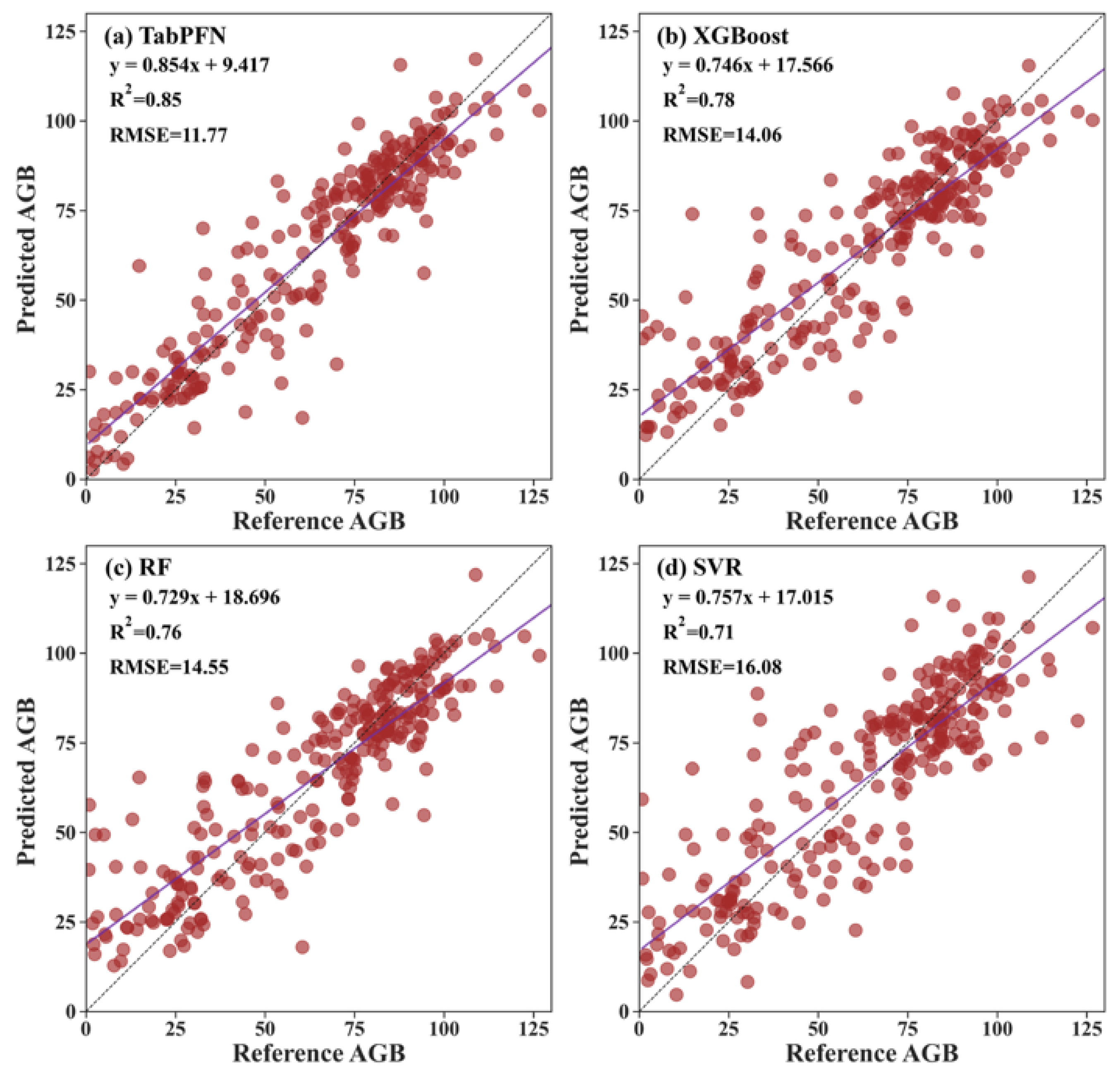
To rigorously verify the models’ true predictive capabilities and rule out the potential overestimation of accuracy caused by spatial autocorrelation, a 10-fold spatial block cross-validation was conducted. Figure 13 presents the spatial cross-validation results for the four models using the optimal multi-source feature combination. TabPFN consistently maintained the highest predictive performance, achieving an R² of 0.85 and an RMSE of 11.77 Mg/ha (Figure 13a). XGBoost (Figure 13b) and random forest (Figure 13c) yielded lower R² values of 0.78 and 0.76, with RMSEs increasing to 14.06 and 14.55 Mg·ha⁻¹, respectively. SVR (Figure 13d) demonstrated the weakest spatial transferability, with R² dropping to 0.71.

3.3.4. SHAP-Based Spatial Analysis

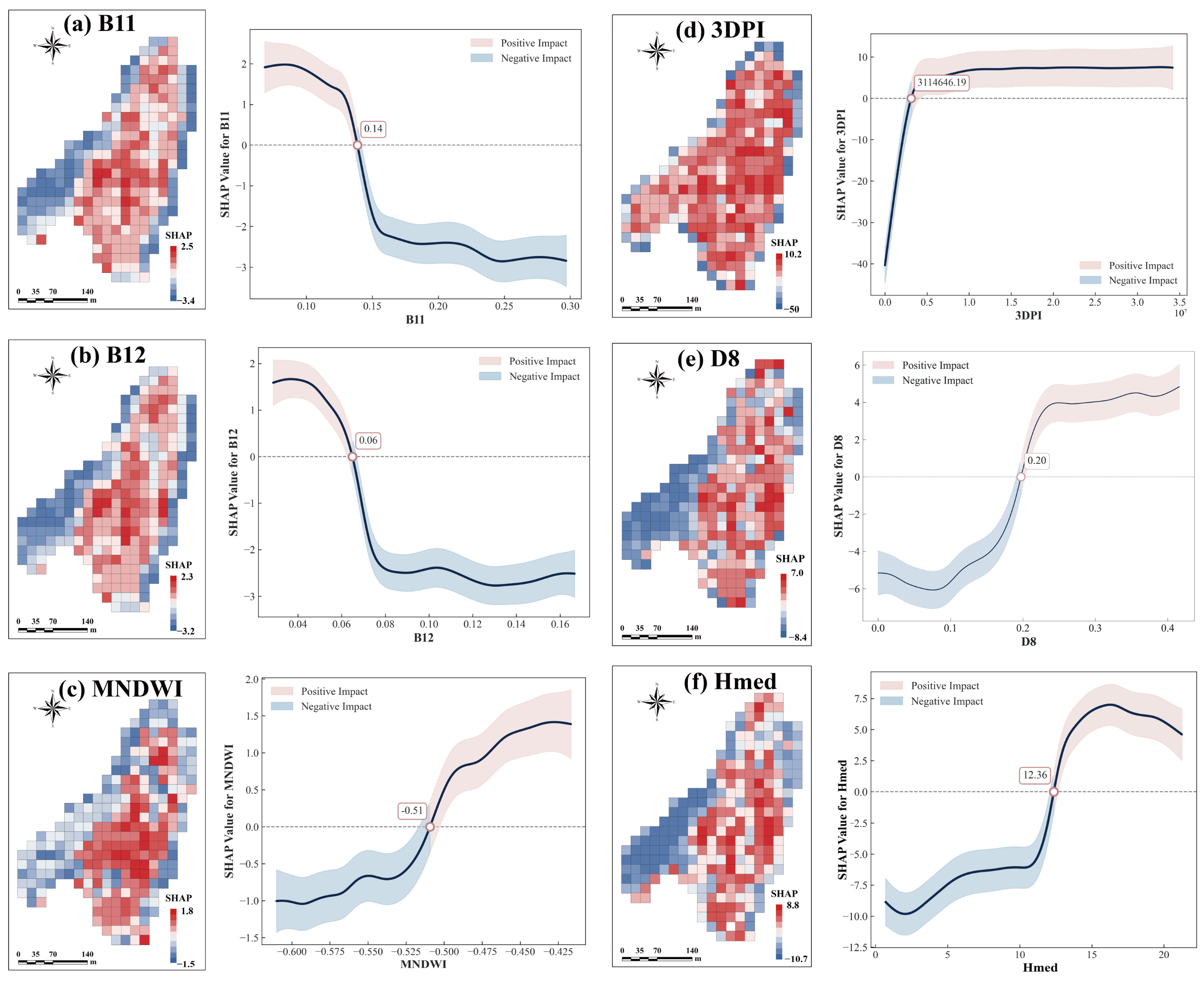
The SHAP interpretation framework transcended traditional black-box predictions by explicitly quantifying the ecological drivers of AGB estimation, with spatial contributions and nonlinear effects illustrated in Figure 14. LiDAR structural variables dominated the model responses. The most influential feature, 3DPI, showed a clear saturation effect, shifting from negative to positive contributions at approximately 3.11 × 10⁶ and stabilizing thereafter. This observed saturation mathematically mirrors the ecological reality that mature Chinese fir stands eventually reach a structural plateau, where further biomass accumulation occurs predominantly via wood densification rather than vertical canopy expansion. Other structural metrics corroborated this structural-driven pattern: D8 exhibited a positive S-shaped response with a threshold near 0.20, indicating that upper-canopy density promoted AGB only beyond this level, while Hmed transitioned to a positive contribution above 12.36 m. Spatially, this resulted in positive contributions from the central and eastern dense stands, whereas western and northern sparse areas were characterized by negative structural contributions.

Concurrently, Sentinel-2 spectral features provided secondary, yet crucial, physiological refinement. SWIR bands displayed inverse S-shaped relationships with thresholds around 0.14 and 0.06, respectively, while MNDWI showed a positive S-shaped response with a threshold near −0.51. These thresholds collectively reflect the strong SWIR absorption and high moisture signals characteristic of high-biomass, water-rich canopies. Ecologically, these optical indices acted as vital physiological discriminators; for stands that shared similar 3D volumetric envelopes (as detected by LiDAR) but differed in successional stages or canopy vitality, Sentinel-2 features effectively fine-tuned the structural baseline, ensuring a more holistic and accurate AGB estimation.

3.3.5. Spatial Distribution of Estimated AGB

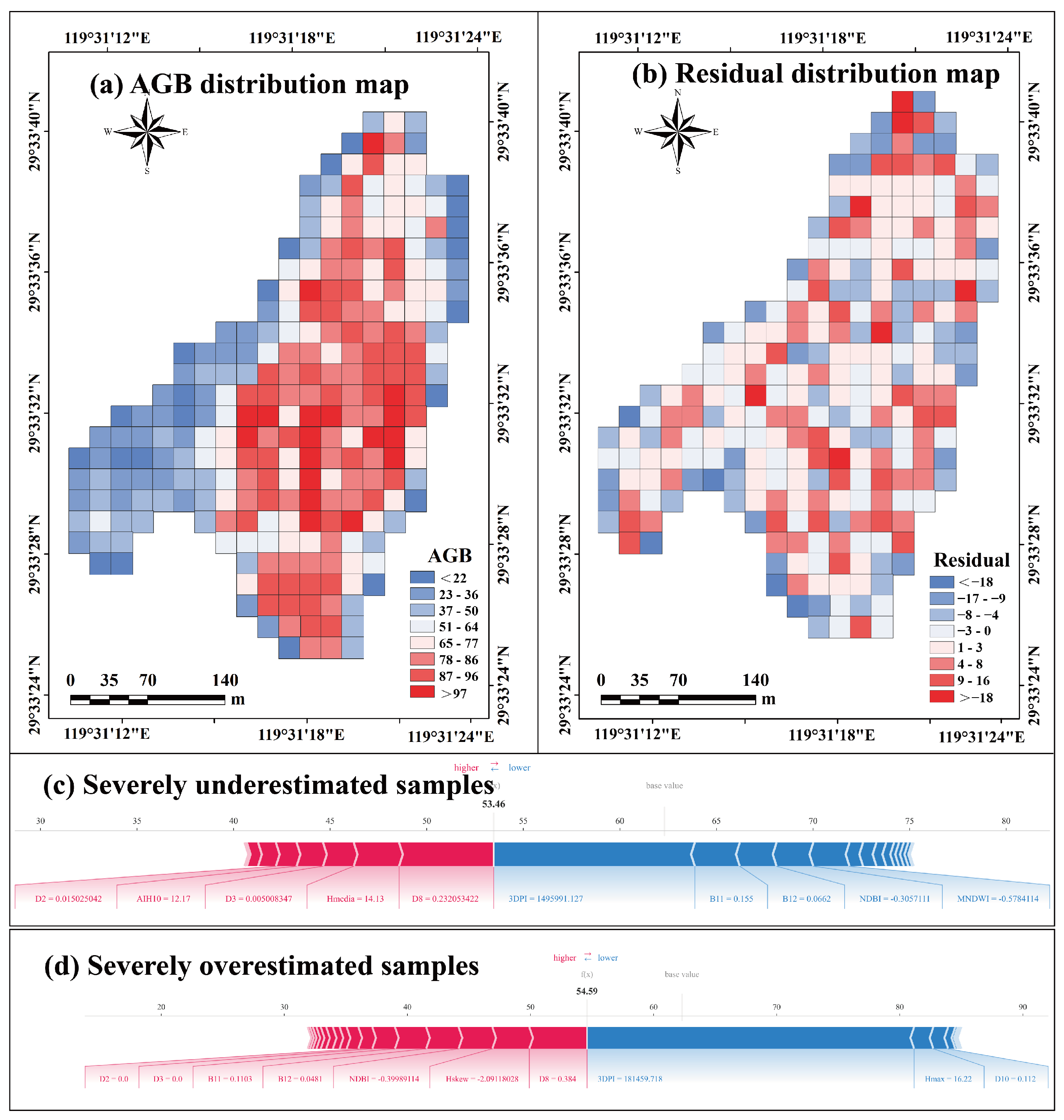
Using the optimal TabPFN model driven by 2 pts/m² simulated LiDAR and Sentinel-2 features, a wall-to-wall AGB map was generated across the study area (Figure 15a). High-biomass stands (>78 Mg·ha⁻¹) were predominantly concentrated in the central-southern and southeastern regions, whereas low-biomass stands (<50 Mg·ha⁻¹) were clustered in the northwest and along the western boundary. This spatial heterogeneity aligns well with local topographical gradients and known stand development stages. Furthermore, the residual distribution (Figure 15b) exhibited no evident spatial autocorrelation, confirming the model’s predictive stability and robust generalization capability across the diverse landscape.

To unravel the ecological mechanisms driving localized prediction errors, SHAP force plots were analyzed for two extreme residual cases (Figure 15c,d). In the severely under-predicted sample (true AGB = 95.02 Mg·ha⁻¹, predicted = 53.46 Mg·ha⁻¹), positive contributions from top-canopy height metrics (Hmed, D8) were overwhelmed by a strongly negative 3DPI signal and suppressed Sentinel-2 spectral features. Ecologically, this reflects an atypical mature stand that has reached its height asymptote but possesses abnormally low internal canopy complexity and weak physiological vigor. Conversely, in the over-predicted sample (true AGB = 12.94 Mg·ha⁻¹, predicted = 54.59 Mg·ha⁻¹), the negative contribution of a low 3DPI was overridden by positive signals from LiDAR upper-canopy metrics (D8, Hskew) and robust Sentinel-2 vegetation indices. This optical-structural combination led the model to misclassify a dense, vigorously growing young stand as a high-biomass mature stand due to its disproportionately closed canopy.

3.4. Uncertainty Quantification and Model Robustness Analysis

3.4.1. Cross-Scale Error Propagation and Stand-Level Predictive Robustness

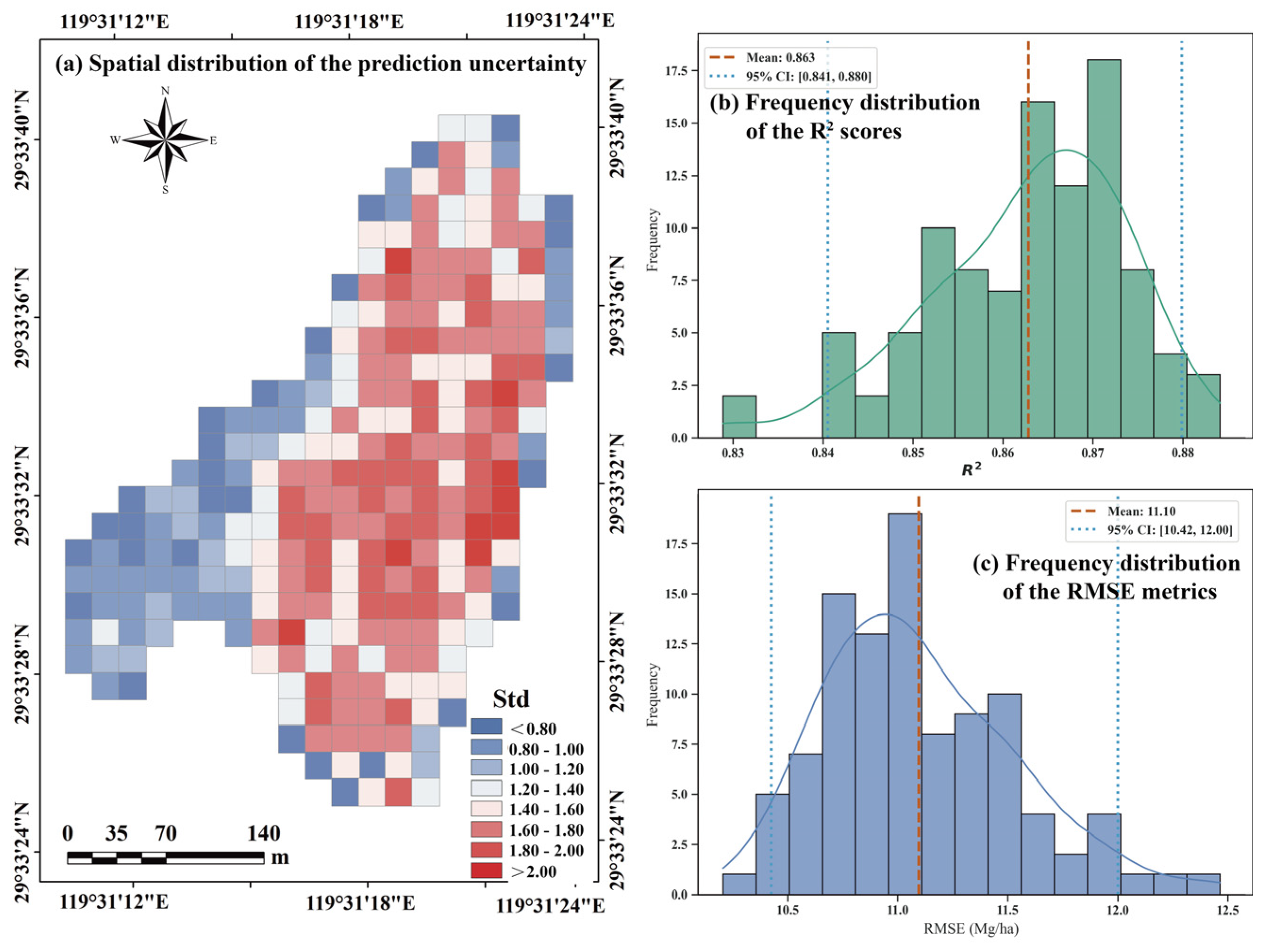
To quantify the propagation of uncertainty from individual-tree predictions to stand-level biomass estimation, the spatial distribution of AGB prediction uncertainty was characterized using the standard deviations (Std) derived from 1000 Monte Carlo simulations (Figure 16a). The uncertainty exhibited clear spatial variability, with higher values generally occurring in areas with greater biomass density. Specifically, the central and eastern plots, which were dominated by mature stands with relatively high biomass, showed higher absolute uncertainty (Std > 1.40 Mg·ha⁻¹). In contrast, sparse stands located along the western and northwestern boundaries exhibited lower uncertainty levels (Std < 1.00 Mg·ha⁻¹). Although uncertainty increased in high-biomass regions, the magnitude of variation remained relatively small compared with the total stand biomass, where AGB values in core areas frequently exceeded 80 Mg·ha⁻¹. The maximum absolute uncertainty was generally maintained below 2.0 Mg·ha⁻¹, indicating limited error amplification during the bottom-up scaling process.

Furthermore, the influence of propagated label uncertainty on stand-level AGB estimation was evaluated using 100 iterations of nested Monte Carlo cross-validation based on the TabPFN model (Figure 16b,c). By incorporating uncertainty into the target variables, the stability of model performance under different realizations of biomass estimates was assessed. The R² values showed a mean of 0.863 with a narrow 95% confidence interval (CI) of 0.841–0.880, while the mean RMSE was 11.10 Mg·ha⁻¹ with a corresponding 95% CI of 10.42–12.00 Mg·ha⁻¹. The relatively concentrated distributions of these evaluation metrics suggest that the integration of simulated LiDAR structural information and Sentinel-2 spectral features provides a stable predictive framework, which remains reliable under uncertainties introduced during the upscaling process.

3.4.2. Probabilistic SHAP Analysis and Feature Ranking Stability

By combining Monte Carlo simulations with SHAP interpretability analysis, we not only revealed the mean contribution of each feature to AGB (Figure 17a), but more importantly, quantitatively evaluated the noise-resistant robustness of feature importance rankings through the heatmap (Figure 17b). Notably, the ranking stability of 3DPI (100% probability of ranking first) strongly proves the decisive role of 3D point cloud structural indicators in retrieving forest biomass, which, combined with Hmed, which securely held second place (97% probability), perfectly corroborates the paper’s core conclusion that LiDAR-derived vertical 3D physical structures dictate the fundamental baseline of biomass accumulation. Meanwhile, spectral features represented by B11 (shortwave infrared), although their specific rankings fluctuated slightly during simulation iterations, always remained firmly in the top tier of importance rankings; this provides solid support for the “structure-physiology” synergistic mechanism of LiDAR-spectral features.

4. Discussion

4.1. Physical Fidelity of LESS Simulation and Density-Dependent Feature Stability

The comparison between the LESS-simulated ALS data and the UAV-LiDAR reference data indicated that the simulation preserved the dominant stand-scale canopy characteristics required for AGB estimation. The strong agreement between the derived canopy height models and key structural metrics suggests that the reconstructed scenes retained the overall canopy envelope and vertical distribution of the Chinese fir stands. By maintaining the underlying forest structure while varying point density, LESS provided a controlled framework for evaluating the sensitivity of LiDAR-derived metrics while reducing interference from differences in acquisition time, flight configuration, and stand conditions [31,32].

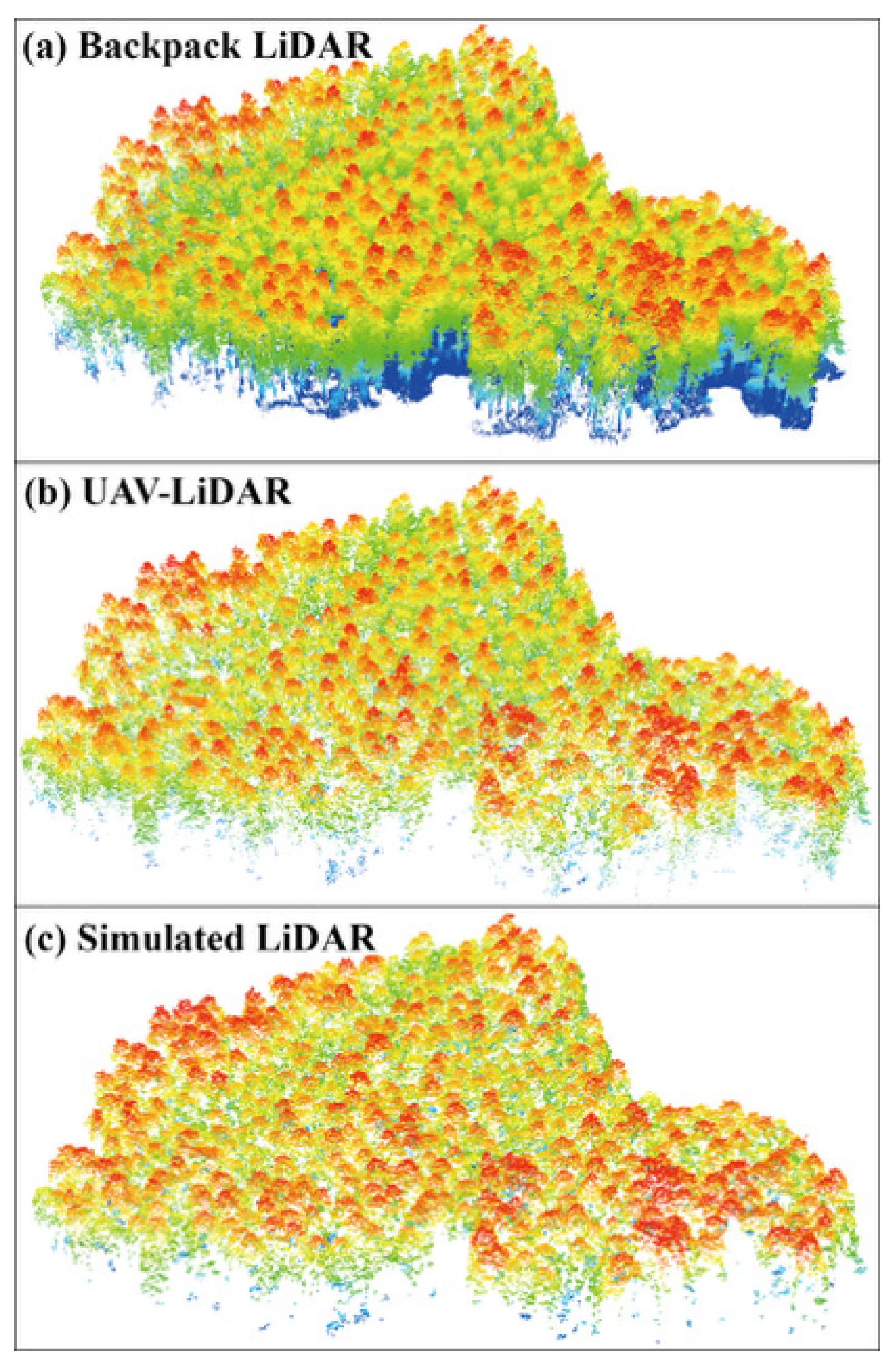
The point clouds shown in Figure 18a–c provide a qualitative illustration of the structural information emphasized by different scanning platforms. In the backpack LiDAR point cloud, stems, lower branches, and understory vegetation were visually more apparent, whereas the UAV-LiDAR and LESS-simulated ALS point clouds primarily emphasized the upper-canopy surface and broad canopy envelope. This contrast primarily reflects differences in viewing geometry and within-canopy occlusion: ground-based scanning observes stems and lower-canopy elements from lateral and upward directions, whereas top-down UAV and airborne scanning encounters the upper crown first, thereby limiting laser penetration and reducing the sampling of lower canopy layers. Although the top-down observations contained less information on internal and lower-canopy structure, the simulated data retained canopy-height and vertical return-distribution characteristics that were influential in stand-level AGB modeling, consistent with the importance of Hmed, D8, and 3DPI. Future integration of ground-based and airborne LiDAR may provide a more complete representation of both internal and external canopy structure by combining their complementary viewing geometries [58,59,60].

The response to point-density reduction differed among structural metrics because of their different dependence on return sampling. In this study, Hmed and Hskew remained relatively stable across the tested density levels. This stability likely reflects that within the tested density range and the 20 m × 20 m spatial support, sufficient returns remained to preserve the central tendency and broad shape of the canopy-height distribution. In contrast, D8 and 3DPI were more sensitive to density reduction. D8 is calculated from the proportion of returns above an upper relative-height threshold; consequently, sparse sampling can change both the number of upper-canopy returns in the numerator and the total return count in the denominator, producing greater variability in the resulting proportion. For 3DPI, lower point density reduces the number of returns available within individual vertical layers, increasing sampling variability in both the layer-specific return proportion and the cumulative return proportion above each layer. Because these two terms jointly determine the weighted contribution of each vertical layer, sparse sampling alters the vertical return profile represented by 3DPI. Therefore, the greater density sensitivity of D8 and 3DPI primarily reflected fluctuations in upper-canopy return proportions and the weighted vertical organization of returns rather than changes in height alone. The increase in AGB prediction accuracy from 0.5 to approximately 2 pts/m², followed by limited gains at 5 and 10 pts/m², suggests that approximately 2 pts/m² provided sufficient sampling to characterize most of the predictive canopy-height, upper-canopy-density, and vertical-distribution information available under the conditions of this study.

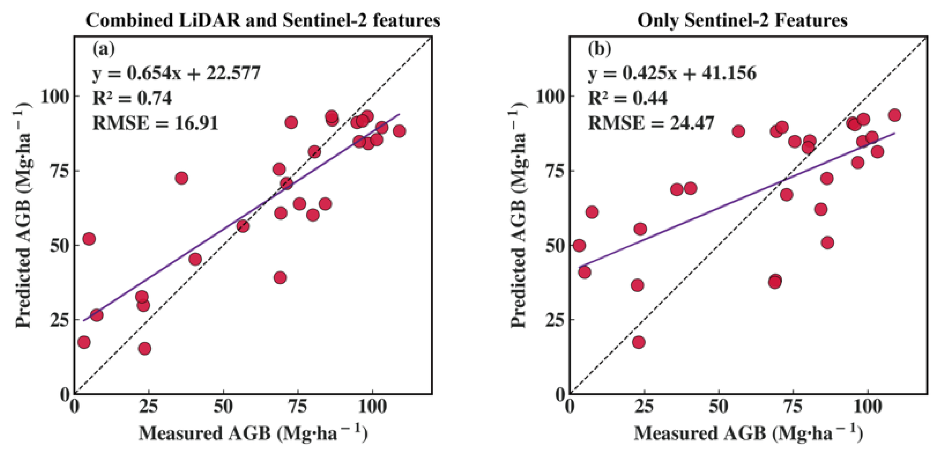
Although LESS simplifies some acquisition and environmental effects present in operational ALS observations, the independent field-plot evaluation showed that the simulated data retained useful AGB-related structural information. The Sentinel-2-only model showed relatively limited performance on the field plots, whereas the integration of simulated ALS structural metrics improved the prediction accuracy (Figure 19). These results support the applicability of LESS-simulated LiDAR for analyzing density-dependent structural information and developing stand-level AGB models under the conditions examined in this study.

4.2. Structural and Spectral Controls on Chinese Fir AGB

The improved performance obtained by integrating LiDAR and Sentinel-2 data reflects their sensitivity to different components of forest canopy properties. Sentinel-2 observations are primarily determined by canopy reflectance, which is influenced by leaf optical properties, crown closure, shadowing, understory conditions, and multiple scattering within the canopy. As Chinese fir stands become denser and biomass increases, visible and near-infrared reflectance tends to approach an asymptotic response because additional woody material beneath the upper canopy contributes little to the signal received by the sensor. Consequently, Sentinel-2 data alone can represent broad spatial variation in canopy condition but provide limited sensitivity to further biomass accumulation in mature, closed-canopy stands, leading to the commonly reported optical saturation problem [61].

LiDAR reduces this limitation by directly characterizing the vertical and three-dimensional organization of the canopy. The dominant LiDAR predictors identified in this study—3DPI, Hmed, and D8—represent complementary dimensions of stand structure. The 3DPI describes the spatial occupancy and vertical concentration of canopy material and therefore increases as tree crowns become more developed and the canopy volume is more fully occupied. Hmed represents the central position of the canopy-height distribution and is related to the dominant vertical stature of the stand while being less sensitive than maximum height to isolated tall trees or anomalous returns. D8 describes the proportion of returns concentrated in the upper canopy and is therefore associated with the development and closure of dominant crowns. Together, these variables characterize canopy volume, vertical stature, and upper-canopy density, all of which are related to tree size, stand development, and the accumulation of woody biomass. This explains why LiDAR-derived structural metrics formed the primary predictive constraint for Chinese fir AGB and remained more informative than optical variables in dense stands.

The nonlinear SHAP responses further indicate that the model-attributed contribution of structural information varied across the observed feature ranges. Lower Hmed values were associated with lower median canopy-return heights, whereas lower D8 values represented smaller proportions of upper-canopy returns. Lower 3DPI values represented differences in the weighted vertical-return profile rather than necessarily lower canopy occupancy. As these variables increased, their SHAP contributions generally became more positive. However, the plateau observed for some variables indicates that additional variation in these metrics contributed progressively less to the fitted model after a threshold was reached. This pattern may reflect the diminishing sensitivity of canopy-based structural metrics in mature or closed-canopy stands, because LiDAR-derived canopy height and vertical-distribution metrics do not fully capture other biomass-related attributes, such as stem diameter and wood properties [62]. Nevertheless, the plateau should be interpreted as saturation of the metric–model relationship rather than the cessation of actual biomass accumulation. In mature stands, additional AGB may continue to accumulate through radial stem growth and increasing woody biomass, even when changes in canopy height or vertical return distribution become comparatively small [63,64,65].

Sentinel-2 variables provided additional information that was not explicitly represented by LiDAR geometry. The importance of B11 and B12 is physically plausible because shortwave-infrared reflectance is sensitive to leaf and canopy water absorption, as well as variations in dry matter, crown shadowing, canopy openness, and background exposure. MNDWI similarly responds to contrasts involving SWIR reflectance and may help distinguish differences in canopy moisture-related optical conditions and canopy-background composition. These variables represent spectral responses jointly affected by canopy water content, foliage properties, crown closure, understory, and illumination conditions. Their contribution therefore lies in distinguishing stands that exhibit similar LiDAR-derived structural envelopes but differ in spectral condition.

The benefit of multi-source integration can thus be understood as an information-complementarity effect. LiDAR establishes the principal structural baseline of AGB by describing canopy height, occupancy, and vertical density, whereas Sentinel-2 refines predictions by adding information on canopy optical and moisture-sensitive conditions. This complementary effect was also observed under low-density LiDAR scenarios, where the inclusion of Sentinel-2 variables improved prediction performance. However, the spectral variables do not reconstruct canopy details that are physically absent from sparse LiDAR data. Instead, they provide an additional and partially independent source of information that reduces ambiguity among stands with similar or incompletely sampled structural metrics [15,66,67].

4.3. Model Comparison and Spatial Transferability

The model comparison showed that TabPFN achieved the highest predictive performance at both the individual-tree and stand levels. At the stand level, integrating LESS-simulated LiDAR structural metrics with Sentinel-2 predictors produced the best predictive performance, and TabPFN generally outperformed RF, XGBoost, and SVR across the evaluated data configurations. These results suggest that algorithm choice contributed to predictive performance in addition to the information contained in the selected predictors. TabPFN’s relative advantage may be related to the inductive bias learned during pretraining on diverse synthetic tabular tasks, allowing its predictions to draw on a previously learned tabular prediction strategy rather than relying exclusively on task-specific fitting from the available samples [19]. This property may be particularly useful for the present dataset, which contained a limited number of reference samples and heterogeneous LiDAR structural and Sentinel-2 spectral predictors. In contrast, the task-specific baseline models were fitted primarily from the samples available in each training set and may therefore have been more sensitive to sample composition and hyperparameter configuration.

PointNet++ showed lower performance than the feature-based models in individual-tree AGB estimation, although it directly used the three-dimensional point clouds. This difference should not be interpreted as evidence that raw point clouds contain less biomass-related information than manually extracted structural metrics. Direct point-cloud learning requires the model to simultaneously infer crown geometry, vertical organization, sampling irregularity, and their relationships with biomass, whereas the extracted LiDAR metrics compress these complex observations into a smaller set of structurally meaningful predictors. With a limited number of measured trees, this compression can improve the signal-to-noise ratio and reduce the risk that the deep network learns acquisition- or segmentation-specific point patterns rather than general biomass relationships. The observed difference therefore reflects the interaction among sample size, model complexity, and input representation rather than a universal advantage of handcrafted features.

Model performance decreased under spatial block cross-validation relative to random holdout validation, although TabPFN retained its relative advantage over the other models. Spatially adjacent plantation plots may share similar structural, spectral, and unmeasured site or management conditions. Random partitioning can therefore assign geographically adjacent and highly similar plots to both the training and evaluation sets, potentially producing optimistic performance estimates when spatial dependence is present [57]. Spatial block cross-validation reduces the influence of this local spatial similarity by evaluating models on geographically clustered plots withheld from model fitting. The resulting performance decline likely reflects both reduced support from nearby observations and the greater difficulty of predicting spatially withheld plots containing structural and spectral predictor combinations that were less well-represented in the training blocks. The spatial validation results should therefore be interpreted as a more stringent assessment of transferability to withheld portions of the study landscape rather than as evidence of a deterioration in the intrinsic quality of the fitted models.

4.4. Uncertainty Propagation and Interpretation Stability

The stand-level reference AGB values derived from the agent plots inherited uncertainty from the individual-tree AGB estimates used in the aggregation process. In this study, Monte Carlo simulations were used to propagate this uncertainty to the stand-level AGB labels. TabPFN maintained comparatively stable predictive performance under the resulting label perturbations, indicating that the modeling framework was relatively robust to uncertainty in individual-tree AGB estimation [68].

Absolute uncertainty was generally greater in mature, high-biomass stands. This pattern primarily results from the nonlinear and cumulative nature of tree-to-stand upscaling: similar proportional errors in tree dimensions generate larger absolute biomass errors for large trees, while errors associated with a small number of dominant individuals can disproportionately affect the aggregated plot value. Crown overlap and the allocation of large boundary trees may further increase uncertainty in structurally dense stands. However, greater absolute uncertainty does not necessarily indicate lower relative reliability, because the propagated error may still account for only a small proportion of the total AGB. Therefore, uncertainty maps should be interpreted together with local biomass magnitude rather than using absolute standard deviation alone.

The probabilistic SHAP analysis further extended uncertainty assessment from model predictions to feature interpretation. The primary LiDAR structural variables maintained relatively stable rankings across Monte Carlo iterations, whereas several secondary structural and spectral predictors showed greater ranking variability. The contrast in ranking stability is likely governed by both signal strength and predictor redundancy: dominant LiDAR metrics represent strong structural gradients in canopy occupancy and vertical development, whereas correlated spectral bands, vegetation indices, and secondary LiDAR metrics contain partially overlapping information. When several correlated variables provide similar predictive information, small perturbations in the AGB labels can redistribute SHAP importance among them without substantially changing the overall model predictions. Thus, fluctuations in the exact rankings of secondary variables do not necessarily imply that they are uninformative; rather, their collective contribution may be more robust than the ordering of individual predictors [69].

Probabilistic SHAP therefore provides a more cautious basis for interpreting multi-source AGB models than a single deterministic ranking. Stable ranking probabilities indicate variables on which the fitted model consistently relies, whereas variable rankings or wider confidence intervals reveal sensitivity to label uncertainty and predictor correlation. Accordingly, the stability of the primary LiDAR variables supports the robustness of the structural information used by the model, while the variability of secondary-feature rankings cautions against assigning ecological significance to their exact ordering. Importantly, SHAP values explain the behavior of the fitted model rather than demonstrating causal ecological relationships. Combining uncertainty propagation with interpretation-stability analysis therefore reduces the risk of overinterpreting a single model realization and provides a more defensible assessment of multi-source predictor contributions.

4.5. Limitations, Practical Implications, and Transferability

The main limitations of this study arise from the use of data from a single Chinese fir plantation region and model-assisted agent plots. Although the agent plots increased the spatial and structural coverage of the reference dataset, their AGB values were aggregated from individual-tree predictions rather than obtained from independent field measurements. In addition, LESS preserved the principal canopy structural patterns required for the point-density experiment but cannot be considered fully equivalent to operational ALS observations.

Despite these limitations, the results provide practical guidance for stand-level AGB inventory. The limited improvement beyond a moderate LiDAR point density indicates that continuously increasing point density may not always be necessary in structurally similar Chinese fir plantations. Height-based metrics remained relatively stable under sparse sampling, whereas density- and voxel-based metrics required more complete point-cloud coverage. Integrating Sentinel-2 with LiDAR further provided complementary spectral information. The practical value of the framework lies in balancing structural information, optical coverage, and acquisition cost rather than simply maximizing LiDAR point density.

Beyond the subtropical Chinese fir plantations examined here, the proposed scale-bridging framework provides a testable basis for evaluating additional Earth observation data sources. Potential extensions include the Global Ecosystem Dynamics Investigation (GEDI), the Ice, Cloud, and land Elevation Satellite-2 (ICESat-2), and spaceborne imaging spectroscopy observations such as EnMAP data [70,71,72]. However, these sensors differ substantially in measurement principle, footprint or sampling geometry, spatial support, and noise characteristics. Extending the LESS framework to GEDI-like waveform observations or ICESat-2-like photon-counting measurements would therefore require sensor-specific modeling of footprint size, along-track sampling, waveform or photon detection, background noise, and geolocation uncertainty. Rather than directly guaranteeing cross-platform integration, physically based simulations could provide controlled experiments for evaluating how structural information changes across sensor configurations and spatial scales before integration with actual satellite observations. Similarly, combining physical simulations with pretrained tabular foundation models may offer a data-efficient strategy for heterogeneous remote sensing datasets, but its effectiveness under shifts in forest type, spatial resolution, sensor geometry, and label quality remains to be tested. Independent validation across forest types, regions, seasons, and operational sensor datasets is therefore required before the framework can be considered transferable across observation platforms.

5. Conclusions

This study successfully resolves the persistent scale mismatch and data scarcity challenges in regional AGB estimation by proposing a novel, scale-consistent framework for subtropical plantations. By synergizing high-density UAV observations, 3D radiative transfer modeling, and foundation-level machine learning, we achieved robust, high-precision, and interpretable stand-level AGB mapping. The primary scientific and methodological contributions are summarized as follows:

(1) A scale-bridging mechanism based on individual-tree upscaling. By utilizing high-density UAV-LiDAR to construct individual-tree AGB models, individual predictions were aggregated to generate stand-level “agent plots”. This bottom-up sample expansion approach mitigated the limitations of limited field data, providing an expanded and spatially distributed reference dataset for regional biomass estimation.

(2) Evaluation of machine learning models for AGB estimation. Among the evaluated algorithms (random forest, XGBoost, SVR, and TabPFN), the TabPFN model achieved the highest predictive accuracy. By integrating multi-source features, TabPFN yielded a stand-level R² of 0.88 and an RMSE of 9.23 Mg·ha⁻¹. Additionally, compared to traditional ensemble methods, TabPFN demonstrated more stable predictive performance under limited sample conditions.

(3) Interpretation of multi-source feature contributions. SHAP analysis was utilized to interpret the relative importance of the predictor variables. The results indicated that LiDAR-derived vertical structural metrics (e.g., 3DPI, Hmed) were the primary predictors for AGB estimation. Meanwhile, Sentinel-2 spectral features, particularly SWIR and moisture indices, provided complementary physiological information. The integration of these structural and spectral features contributed to mitigating the limitations of single-sensor data, such as optical saturation in dense stands.

(4) Uncertainty quantification in AGB upscaling. Monte Carlo simulations were applied to quantify the error propagation from individual-tree predictions to stand-level AGB. The uncertainty mapping indicated that absolute variance was relatively higher in mature, high-biomass stands. Despite the introduced label noise, the model maintained stable predictive performance. Additionally, the probabilistic SHAP analysis evaluated the ranking stability of feature importance, confirming the consistent contribution of primary LiDAR structural metrics (e.g., 3DPI) under noisy conditions and providing an objective basis for feature evaluation.

References

1. Baccini, A.; Walker, W.; Carvalho, L.; Farina, M.; Sulla-Menashe, D.; Houghton, R.A. Tropical Forests Are a Net Carbon Source Based on Aboveground Measurements of Gain and Loss. Science 2017, 358, 230–234. [Google Scholar] [CrossRef] [Scilit] [PubMed]
2. Saatchi, S.S.; Harris, N.L.; Brown, S.; Lefsky, M.; Mitchard, E.T.A.; Salas, W.; Zutta, B.R.; Buermann, W.; Lewis, S.L.; Hagen, S.; et al. Benchmark Map of Forest Carbon Stocks in Tropical Regions Across Three Continents. Proc. Natl. Acad. Sci. USA 2011, 108, 9899–9904. [Google Scholar] [CrossRef] [Scilit] [PubMed]
3. Zhu, X.; Liu, D. Improving Forest Aboveground Biomass Estimation Using Seasonal Landsat NDVI Time-Series. ISPRS J. Photogramm. Remote Sens. 2015, 102, 222–231. [Google Scholar] [CrossRef] [Scilit]
4. Su, Y.; Guo, Q.; Xue, B.; Hu, T.; Alvarez, O.; Tao, S.; Fang, J. Spatial Distribution of Forest Aboveground Biomass in China: Estimation Through Combination of Spaceborne Lidar, Optical Imagery, and Forest Inventory Data. Remote Sens. Environ. 2016, 173, 187–199. [Google Scholar] [CrossRef] [Scilit]
5. Pelletier, F.; Cardille, J.A.; Wulder, M.A.; White, J.C.; Hermosilla, T. Inter- and Intra-Year Forest Change Detection and Monitoring of Aboveground Biomass Dynamics Using Sentinel-2 and Landsat. Remote Sens. Environ. 2024, 301, 113931. [Google Scholar] [CrossRef] [Scilit]
6. David, R.M.; Rosser, N.J.; Donoghue, D.N.M. Improving Above Ground Biomass Estimates of Southern Africa Dryland Forests by Combining Sentinel-1 SAR and Sentinel-2 Multispectral Imagery. Remote Sens. Environ. 2022, 282, 113232. [Google Scholar] [CrossRef] [Scilit]
7. Vaglio Laurin, G.; Chen, Q.; Lindsell, J.A.; Coomes, D.A.; Frate, F.D.; Guerriero, L.; Pirotti, F.; Valentini, R. Above Ground Biomass Estimation in an African Tropical Forest with Lidar and Hyperspectral Data. ISPRS J. Photogramm. Remote Sens. 2014, 89, 49–58. [Google Scholar] [CrossRef] [Scilit]
8. Cao, Y.; Zhao, Y.; Xu, J.; Fang, Q.; Xuan, J.; Huang, L.; Li, X.; Mao, F.; Sun, Y.; Du, H. UAV-LiDAR-Based Study on AGB Response to Stand Structure and Its Estimation in Cunninghamia lanceolata Plantations. Remote Sens. 2025, 17, 2842. [Google Scholar] [CrossRef] [Scilit]
9. Zhang, L.; Zhao, Y.; Chen, C.; Li, X.; Mao, F.; Lv, L.; Yu, J.; Song, M.; Huang, L.; Chen, J.; et al. UAV-LiDAR Integration with Sentinel-2 Enhances Precision in AGB Estimation for Bamboo Forests. Remote Sens. 2024, 16, 705. [Google Scholar] [CrossRef] [Scilit]
10. Coops, N.C.; Tompalski, P.; Goodbody, T.R.H.; Queinnec, M.; Luther, J.E.; Bolton, D.K.; White, J.C.; Wulder, M.A.; van Lier, O.R.; Hermosilla, T. Modelling Lidar-Derived Estimates of Forest Attributes over Space and Time: A Review of Approaches and Future Trends. Remote Sens. Environ. 2021, 260, 112477. [Google Scholar] [CrossRef] [Scilit]
11. Zhang, B.; Li, X.; Du, H.; Zhou, G.; Mao, F.; Huang, Z.; Zhou, L.; Xuan, J.; Gong, Y.; Chen, C. Estimation of Urban Forest Characteristic Parameters Using UAV-Lidar Coupled with Canopy Volume. Remote Sens. 2022, 14, 6375. [Google Scholar] [CrossRef] [Scilit]
12. Duncanson, L.I.; Dubayah, R.O.; Cook, B.D.; Rosette, J.; Parker, G. The Importance of Spatial Detail: Assessing the Utility of Individual Crown Information and Scaling Approaches for Lidar-Based Biomass Density Estimation. Remote Sens. Environ. 2015, 168, 102–112. [Google Scholar] [CrossRef] [Scilit]
13. Luo, Z.; Zhang, Z.; Li, W.; Chen, Y.; Wang, C.; Nurunnabi, A.A.M.; Li, J. Detection of Individual Trees in UAV LiDAR Point Clouds Using a Deep Learning Framework Based on Multichannel Representation. IEEE Trans. Geosci. Remote Sens. 2022, 60, 1–15. [Google Scholar] [CrossRef] [Scilit]
14. Brede, B.; Terryn, L.; Barbier, N.; Bartholomeus, H.M.; Bartolo, R.; Calders, K.; Derroire, G.; Krishna Moorthy, S.M.; Lau, A.; Levick, S.R.; et al. Non-Destructive Estimation of Individual Tree Biomass: Allometric Models, Terrestrial and UAV Laser Scanning. Remote Sens. Environ. 2022, 280, 113180. [Google Scholar] [CrossRef] [Scilit]
15. Wang, D.; Wan, B.; Liu, J.; Su, Y.; Guo, Q.; Qiu, P.; Wu, X. Estimating Aboveground Biomass of the Mangrove Forests on Northeast Hainan Island in China Using an Upscaling Method from Field Plots, UAV-LiDAR Data and Sentinel-2 Imagery. Int. J. Appl. Earth Obs. Geoinf. 2020, 85, 101986. [Google Scholar] [CrossRef] [Scilit]
16. Meng, B.; Liang, T.; Yi, S.; Yin, J.; Cui, X.; Ge, J.; Hou, M.; Lv, Y.; Sun, Y. Modeling Alpine Grassland Above Ground Biomass Based on Remote Sensing Data and Machine Learning Algorithm: A Case Study in East of the Tibetan Plateau, China. IEEE J. Sel. Top. Appl. Earth Obs. Remote Sens. 2020, 13, 2986–2995. [Google Scholar] [CrossRef] [Scilit]
17. Naik, P.; Dalponte, M.; Bruzzone, L. Automated Machine Learning Driven Stacked Ensemble Modeling for Forest Aboveground Biomass Prediction Using Multitemporal Sentinel-2 Data. IEEE J. Sel. Top. Appl. Earth Obs. Remote Sens. 2023, 16, 3442–3454. [Google Scholar] [CrossRef] [Scilit]
18. Song, C.; Li, Z.; Dai, Y.; Liu, T.; Li, J. Estimation of Forest Aboveground Biomass in North China Based on Landsat Data and Stand Features. Forests 2025, 16, 384. [Google Scholar] [CrossRef] [Scilit]
19. Hollmann, N.; Müller, S.; Purucker, L.; Krishnakumar, A.; Körfer, M.; Hoo, S.B.; Schirrmeister, R.T.; Hutter, F. Accurate Predictions on Small Data with a Tabular Foundation Model. Nature 2025, 637, 319–326. [Google Scholar] [CrossRef] [Scilit] [PubMed]
20. Lundberg, S.M.; Lee, S.-I. A Unified Approach to Interpreting Model Predictions. In Proceedings of the Advances in Neural Information Processing Systems; Curran Associates, Inc.: Red Hook, NY, USA, 2017; Volume 30. [Google Scholar]
21. Lundberg, S.M.; Erion, G.; Chen, H.; DeGrave, A.; Prutkin, J.M.; Nair, B.; Katz, R.; Himmelfarb, J.; Bansal, N.; Lee, S.-I. From Local Explanations to Global Understanding with Explainable AI for Trees. Nat. Mach. Intell. 2020, 2, 56–67. [Google Scholar] [CrossRef] [Scilit] [PubMed]
22. Li, X.; Du, H.; Mao, F.; Xu, Y.; Huang, Z.; Xuan, J.; Zhou, Y.; Hu, M. Estimation Aboveground Biomass in Subtropical Bamboo Forests Based on an Interpretable Machine Learning Framework. Environ. Model. Softw. 2024, 178, 106071. [Google Scholar] [CrossRef] [Scilit]
23. Li, X.; Ramos Aguila, L.C.; Wu, D.; Lie, Z.; Xu, W.; Tang, X.; Liu, J. Carbon Sequestration and Storage Capacity of Chinese Fir at Different Stand Ages. Sci. Total Environ. 2023, 904, 166962. [Google Scholar] [CrossRef] [Scilit] [PubMed]
24. Chen, A.; Zhao, P.; Li, Y.; He, H.; Zhang, G.; Li, T.; Liu, Y.; Wen, X. Estimation and Spatial Distribution of Individual Tree Aboveground Biomass in a Chinese Fir Plantation in the Dabieshan Mountains of Western Anhui, China. Forests 2024, 15, 1743. [Google Scholar] [CrossRef] [Scilit]
25. Hu, Y.; Fu, L.; Qiu, B.; Xie, D.; Wu, Z.; Lei, Y.; Ye, J.; Wang, Q. Uncertainty Analysis of Remote Sensing Estimation of Chinese Fir (Cunninghamia lanceolata) Aboveground Biomass in Southern China. Forests 2025, 16, 230. [Google Scholar] [CrossRef] [Scilit]
26. Huang, X.; Chen, Y.; Tan, H.; Zhang, Y.; Yu, S.; Chen, X.; Yu, K.; Liu, J. Extraction of the Spatial Structure of Chinese Fir Plantations Stands Based on Unmanned Aerial Vehicle and Its Effect on AGB. For. Ecol. Manag. 2024, 558, 121800. [Google Scholar] [CrossRef] [Scilit]
27. Tao, Y.; Shen, X.; Fan, F.; Ye, D.; Zhang, L.; Cao, L. The Estimation of Tree-Level Key Structural Parameters Based on ULS and BLS Point Clouds by Evaluating Prediction Accuracy from Tree Stem Analysis. Comput. Electron. Agric. 2026, 246, 111668. [Google Scholar] [CrossRef] [Scilit]
28. Qin, L.; Zhang, M.; Zhong, S.; Yu, X. Model Uncertainty in Forest Biomass Estimation. Acta Ecol. Sin. 2017, 37, 7912–7919. [Google Scholar] [CrossRef] [Scilit]
29. Zhao, X.; Guo, Q.; Su, Y.; Xue, B. Improved Progressive TIN Densification Filtering Algorithm for Airborne LiDAR Data in Forested Areas. ISPRS J. Photogramm. Remote Sens. 2016, 117, 79–91. [Google Scholar] [CrossRef] [Scilit]
30. Li, W.; Guo, Q.; Jakubowski, M.K.; Kelly, M. A New Method for Segmenting Individual Trees from the Lidar Point Cloud. Photogramm. Eng. Remote Sens. 2012, 78, 75–84. [Google Scholar] [CrossRef] [Scilit]
31. Qi, J.; Xie, D.; Yin, T.; Yan, G.; Gastellu-Etchegorry, J.-P.; Li, L.; Zhang, W.; Mu, X.; Norford, L.K. LESS: LargE-Scale Remote Sensing Data and Image Simulation Framework over Heterogeneous 3D Scenes. Remote Sens. Environ. 2019, 221, 695–706. [Google Scholar] [CrossRef] [Scilit]
32. Luo, Y.; Xie, D.; Qi, J.; Zhou, K.; Yan, G.; Mu, X. LESS LiDAR: A Full-Waveform and Discrete-Return Multispectral LiDAR Simulator Based on Ray Tracing Algorithm. Remote Sens. 2023, 15, 4529. [Google Scholar] [CrossRef] [Scilit]
33. Qi, J.; Xie, D.; Jiang, J.; Huang, H. 3D Radiative Transfer Modeling of Structurally Complex Forest Canopies Through a Lightweight Boundary-Based Description of Leaf Clusters. Remote Sens. Environ. 2022, 283, 113301. [Google Scholar] [CrossRef] [Scilit]
34. Widlowski, J.-L.; Côté, J.-F.; Béland, M. Abstract Tree Crowns in 3D Radiative Transfer Models: Impact on Simulated Open-Canopy Reflectances. Remote Sens. Environ. 2014, 142, 155–175. [Google Scholar] [CrossRef] [Scilit]
35. Li, W.; Guo, Q.; Tao, S.; Su, Y. VBRT: A Novel Voxel-Based Radiative Transfer Model for Heterogeneous Three-Dimensional Forest Scenes. Remote Sens. Environ. 2018, 206, 318–335. [Google Scholar] [CrossRef] [Scilit]
36. Liao, K.; Li, Y.; Zou, B.; Li, D.; Lu, D. Examining the Role of UAV Lidar Data in Improving Tree Volume Calculation Accuracy. Remote Sens. 2022, 14, 4410. [Google Scholar] [CrossRef] [Scilit]
37. Zhou, L.; Li, X.; Zhang, B.; Xuan, J.; Gong, Y.; Tan, C.; Huang, H.; Du, H. Estimating 3D Green Volume and Aboveground Biomass of Urban Forest Trees by UAV-Lidar. Remote Sens. 2022, 14, 5211. [Google Scholar] [CrossRef] [Scilit]
38. Jimenez-Berni, J.A.; Deery, D.M.; Rozas-Larraondo, P.; Condon, A.T.G.; Rebetzke, G.J.; James, R.A.; Bovill, W.D.; Furbank, R.T.; Sirault, X.R.R. High Throughput Determination of Plant Height, Ground Cover, and Above-Ground Biomass in Wheat with LiDAR. Front. Plant Sci. 2018, 9, 237. [Google Scholar] [CrossRef] [Scilit] [PubMed]
39. Tucker, C.J.; Elgin, J.H.; McMurtrey, J.E.; Fan, C.J. Monitoring Corn and Soybean Crop Development with Hand-Held Radiometer Spectral Data. Remote Sens. Environ. 1979, 8, 237–248. [Google Scholar] [CrossRef] [Scilit]
40. Huete, A.; Didan, K.; Miura, T.; Rodriguez, E.P.; Gao, X.; Ferreira, L.G. Overview of the Radiometric and Biophysical Performance of the MODIS Vegetation Indices. Remote Sens. Environ. 2002, 83, 195–213. [Google Scholar] [CrossRef] [Scilit]
41. Broge, N.H.; Leblanc, E. Comparing Prediction Power and Stability of Broadband and Hyperspectral Vegetation Indices for Estimation of Green Leaf Area Index and Canopy Chlorophyll Density. Remote Sens. Environ. 2001, 76, 156–172. [Google Scholar] [CrossRef] [Scilit]
42. Thorp, K.; Tian, L.F.; Yao, H.; Tang, L. Narrow-Band and Derivative-Based Vegetation Indices for Hyperspectral Data. Trans. ASAE 2004, 47, 291–299. [Google Scholar] [CrossRef] [Scilit]
43. Ren, S.; Chen, X.; An, S. Assessing Plant Senescence Reflectance Index-Retrieved Vegetation Phenology and Its Spatiotemporal Response to Climate Change in the Inner Mongolian Grassland. Int. J. Biometeorol. 2017, 61, 601–612. [Google Scholar] [CrossRef] [Scilit] [PubMed]
44. Chen, D.; Huang, J.; Jackson, T.J. Vegetation Water Content Estimation for Corn and Soybeans Using Spectral Indices Derived from MODIS Near- and Short-Wave Infrared Bands. Remote Sens. Environ. 2005, 98, 225–236. [Google Scholar] [CrossRef] [Scilit]
45. Gao, B. NDWI—A Normalized Difference Water Index for Remote Sensing of Vegetation Liquid Water from Space. Remote Sens. Environ. 1996, 58, 257–266. [Google Scholar] [CrossRef] [Scilit]
46. Rouse, J.W.; Haas, R.H.; Schell, J.A.; Deering, D.W. Monitoring Vegetation Systems in the Great Plains with ERTS; NASA: Washington, DC, USA, 1974. [Google Scholar]
47. Xu, H. Modification of Normalised Difference Water Index (NDWI) to Enhance Open Water Features in Remotely Sensed Imagery. Int. J. Remote Sens. 2006, 27, 3025–3033. [Google Scholar] [CrossRef] [Scilit]
48. Zha, Y.; Gao, J.; Ni, S. Use of Normalized Difference Built-up Index in Automatically Mapping Urban Areas from TM Imagery. Int. J. Remote Sens. 2003, 24, 583–594. [Google Scholar] [CrossRef] [Scilit]
49. Gitelson, A.A.; Viña, A.; Ciganda, V.; Rundquist, D.C.; Arkebauer, T.J. Remote Estimation of Canopy Chlorophyll Content in Crops. Geophys. Res. Lett. 2005, 32, L08403. [Google Scholar] [CrossRef] [Scilit]
50. Haralick, R.M.; Shanmugam, K.; Dinstein, I. Textural Features for Image Classification. IEEE Trans. Syst. Man Cybern. 1973, SMC-3, 610–621. [Google Scholar] [CrossRef] [Scilit]
51. Conners, R.W.; Trivedi, M.M.; Harlow, C.A. Segmentation of a High-Resolution Urban Scene Using Texture Operators. Comput. Vis. Graph. Image Process. 1984, 25, 273–310. [Google Scholar] [CrossRef] [Scilit]
52. Kursa, M.B.; Rudnicki, W.R. Feature Selection with the Boruta Package. J. Stat. Softw. 2010, 36, 1–13. [Google Scholar] [CrossRef] [Scilit]
53. Vapnik, V.; Golowich, S.; Smola, A. Support Vector Method for Function Approximation, Regression Estimation and Signal Processing. In Proceedings of the Advances in Neural Information Processing Systems; MIT Press: Cambridge, MA, USA, 1996; Volume 9. [Google Scholar]
54. Breiman, L. Random Forests. Mach. Learn. 2001, 45, 5–32. [Google Scholar] [CrossRef] [Scilit]
55. Chen, T.; Guestrin, C. XGBoost: A Scalable Tree Boosting System. In Proceedings of the 22nd ACM SIGKDD International Conference on Knowledge Discovery and Data Mining; Association for Computing Machinery: New York, NY, USA, 2016; pp. 785–794. [Google Scholar]
56. Qi, C.R.; Yi, L.; Su, H.; Guibas, L. PointNet++: Deep Hierarchical Feature Learning on Point Sets in a Metric Space. Adv. Neural Inf. Process. Syst. 2017, 30, 5099–5108. [Google Scholar]
57. Roberts, D.R.; Bahn, V.; Ciuti, S.; Boyce, M.S.; Elith, J.; Guillera-Arroita, G.; Hauenstein, S.; Lahoz-Monfort, J.J.; Schröder, B.; Thuiller, W.; et al. Cross-Validation Strategies for Data with Temporal, Spatial, Hierarchical, or Phylogenetic Structure. Ecography 2017, 40, 913–929. [Google Scholar] [CrossRef] [Scilit]
58. Calders, K.; Adams, J.; Armston, J.; Bartholomeus, H.; Bauwens, S.; Bentley, L.P.; Chave, J.; Danson, F.M.; Demol, M.; Disney, M.; et al. Terrestrial Laser Scanning in Forest Ecology: Expanding the Horizon. Remote Sens. Environ. 2020, 251, 112102. [Google Scholar] [CrossRef] [Scilit]
59. Terryn, L.; Calders, K.; Bartholomeus, H.; Bartolo, R.E.; Brede, B.; D’hont, B.; Disney, M.; Herold, M.; Lau, A.; Shenkin, A.; et al. Quantifying Tropical Forest Structure through Terrestrial and UAV Laser Scanning Fusion in Australian Rainforests. Remote Sens. Environ. 2022, 271, 112912. [Google Scholar] [CrossRef] [Scilit]
60. Puletti, N.; Grotti, M.; Masini, A.; Bracci, A.; Ferrara, C. Enhancing Wall-to-Wall Forest Structure Mapping Through Detailed Co-Registration of Airborne and Terrestrial Laser Scanning Data in Mediterranean Forests. Ecol. Inform. 2022, 67, 101497. [Google Scholar] [CrossRef] [Scilit]
61. Xu, X.; Yang, J.; Qi, S.; Ma, Y.; Liu, W.; Li, L.; Lu, X.; Liu, Y. Estimation of Forest Aboveground Biomass Using Sentinel-1/2 Synergized with Extrapolated Parameters from LiDAR Data and Analysis of Its Ecological Driving Factors. Remote Sens. 2025, 17, 2358. [Google Scholar] [CrossRef] [Scilit]
62. Knapp, N.; Fischer, R.; Cazcarra-Bes, V.; Huth, A. Structure Metrics to Generalize Biomass Estimation from Lidar across Forest Types from Different Continents. Remote Sens. Environ. 2020, 237, 111597. [Google Scholar] [CrossRef] [Scilit]
63. Sillett, S.C.; Van Pelt, R.; Koch, G.W.; Ambrose, A.R.; Carroll, A.L.; Antoine, M.E.; Mifsud, B.M. Increasing Wood Production through Old Age in Tall Trees. For. Ecol. Manag. 2010, 259, 976–994. [Google Scholar] [CrossRef] [Scilit]
64. Stephenson, N.L.; Das, A.J.; Condit, R.; Russo, S.E.; Baker, P.J.; Beckman, N.G.; Coomes, D.A.; Lines, E.R.; Morris, W.K.; Rüger, N.; et al. Rate of Tree Carbon Accumulation Increases Continuously with Tree Size. Nature 2014, 507, 90–93. [Google Scholar] [CrossRef] [Scilit] [PubMed]
65. Zhou, L.; Shalom, A.-D.D.; Wu, P.; He, Z.; Liu, C.; Ma, X. Biomass Production, Nutrient Cycling and Distribution in Age-Sequence Chinese Fir (Cunninghamia lanceolate) Plantations in Subtropical China. J. For. Res. 2016, 27, 357–368. [Google Scholar] [CrossRef] [Scilit]
66. Yang, Q.; Su, Y.; Hu, T.; Jin, S.; Liu, X.; Niu, C.; Liu, Z.; Kelly, M.; Wei, J.; Guo, Q. Allometry-Based Estimation of Forest Aboveground Biomass Combining LiDAR Canopy Height Attributes and Optical Spectral Indexes. For. Ecosyst. 2022, 9, 100059. [Google Scholar] [CrossRef] [Scilit]
67. Jiang, F.; Deng, M.; Tang, J.; Fu, L.; Sun, H. Integrating Spaceborne LiDAR and Sentinel-2 Images to Estimate Forest Aboveground Biomass in Northern China. Carbon Balance Manag. 2022, 17, 12. [Google Scholar] [CrossRef] [Scilit] [PubMed]
68. Vorster, A.G.; Evangelista, P.H.; Stovall, A.E.L.; Ex, S. Variability and Uncertainty in Forest Biomass Estimates from the Tree to Landscape Scale: The Role of Allometric Equations. Carbon Balance Manag. 2020, 15, 8. [Google Scholar] [CrossRef] [Scilit] [PubMed]
69. Aas, K.; Jullum, M.; Løland, A. Explaining Individual Predictions When Features Are Dependent: More Accurate Approximations to Shapley Values. Artif. Intell. 2021, 298, 103502. [Google Scholar] [CrossRef] [Scilit]
70. Dubayah, R.; Blair, J.B.; Goetz, S.; Fatoyinbo, L.; Hansen, M.; Healey, S.P.; Hofton, M.; Hurtt, G.; Kellner, J.; Luthcke, S.; et al. The Global Ecosystem Dynamics Investigation: High-Resolution Laser Ranging of the Earth’s Forests and Topography. Sci. Remote Sens. 2020, 1, 100002. [Google Scholar] [CrossRef] [Scilit]
71. Markus, T.; Neumann, T.; Martino, A.; Abdalati, W.; Brunt, K.; Csatho, B.; Farrell, S.; Fricker, H.; Gardner, A.; Harding, D.; et al. The Ice, Cloud, and Land Elevation Satellite-2 (ICESat-2): Science Requirements, Concept, and Implementation. Remote Sens. Environ. 2017, 190, 260–273. [Google Scholar] [CrossRef] [Scilit]
72. Guanter, L.; Kaufmann, H.; Segl, K.; Foerster, S.; Rogass, C.; Chabrillat, S.; Kuester, T.; Hollstein, A.; Rossner, G.; Chlebek, C.; et al. The EnMAP Spaceborne Imaging Spectroscopy Mission for Earth Observation. Remote Sens. 2015, 7, 8830–8857. [Google Scholar] [CrossRef] [Scilit]
Figure 1. Study area: (a) location of Jiande City, (b) field plots and agent plots, (c) height-normalized UAV-LiDAR point cloud colored according to height above ground, and (d) Sentinel-2 false-color composite.
Remotesensing 18 02749 g001
Figure 2. Architecture of the PointNet++ model for individual-tree AGB estimation: (a) overall network pipeline, (b) multi-scale grouping and local feature extraction, and (c) global feature aggregation, and (d) regression head.
Remotesensing 18 02749 g002
Figure 3. Technical workflow.
Remotesensing 18 02749 g003
Figure 4. Comparison between simulated ALS and reference ALS cross-sections: (a) Simulated ALS cross-Section 1, (b) reference ALS cross-Section 1, (c) simulated ALS cross-Section 2, and (d) reference ALS cross-Section 2.
Remotesensing 18 02749 g004
Figure 5. Correlation analysis between CHMs derived from the simulated ALS and reference ALS at different spatial resolutions: (a) 0.5 m, (b) 1 m, and (c) 2 m.
Remotesensing 18 02749 g005
Figure 6. Correlation analysis between structural metrics derived from the simulated ALS and reference ALS.
Remotesensing 18 02749 g006
Figure 7. Effects of simulated ALS point-cloud density on structural feature extraction.
Remotesensing 18 02749 g007
Figure 8. Feature selection results for individual-tree AGB.
Remotesensing 18 02749 g008
Figure 9. Individual-tree AGB estimation results using different models: (a) SVR, (b) XGBoost, (c) RF, (d) TabPFN, and (e) Pointnet++.
Remotesensing 18 02749 g009
Figure 10. Stand-level AGB feature selection results based on the simulated ALS data: (a) 0.5 pts/m2, (b) 1 pts/m2, (c) 2 pts/m2, (d) 5 pts/m2, (e) 10 pts/m2, and (f) Sentinel-2.
Remotesensing 18 02749 g010
Figure 11. Stand-level AGB feature selection results based on the fusion of simulated ALS and Sentinel-2 data: (a) 0.5 pts/m2, (b) 1 pts/m2, (c) 2 pts/m2, (d) 5 pts/m2, and (e) 10 pts/m2.
Remotesensing 18 02749 g011
Figure 12. Stand-level AGB estimation results based on Sentinel-2 data alone as well as under varying LiDAR point densities and data combinations.
Remotesensing 18 02749 g012
Figure 13. Scatter plots of the stand-level AGB predictions versus reference AGB under the 10-fold spatial block cross-validation: (a) TabPFN, (b) XGBoost, (c) RF, and (d) SVR.
Remotesensing 18 02749 g013
Figure 14. Feature interpretation for stand-level AGB: (a) B11, (b) B12, (c) MNDWI, (d) 3DPI, (e) D8, and (f) Hmed.
Remotesensing 18 02749 g014
Figure 15. Spatial mapping of stand-level AGB: (a) AGB distribution map, (b) residual distribution map, (c) severely underestimated samples by the model, and (d) severely overestimated samples by the model.
Remotesensing 18 02749 g015
Figure 16. Spatial mapping of uncertainty and Monte Carlo validation distributions for stand-level AGB estimation. (a) Spatial distribution of the prediction uncertainty. (b) Frequency distribution of the R2 scores from the nested Monte Carlo cross-validation. (c) Frequency distribution of the RMSE metrics from the nested Monte Carlo cross-validation.
Remotesensing 18 02749 g016
Figure 17. Feature importance and ranking robustness analysis accounting for target variable uncertainty. (a) Mean absolute SHAP values and their 95% confidence intervals for each feature under Monte Carlo simulations. (b) Probability distribution heatmap of feature importance rankings across 100 iterations.
Remotesensing 18 02749 g017
Figure 18. Visual comparison of forest point clouds derived from different platforms: (a) backpack LiDAR, (b) UAV-LiDAR, and (c) simulated LiDAR.
Remotesensing 18 02749 g018
Figure 19. Stand-level AGB prediction performance of the agent-plot–trained model when applied to real field plots using (a) LiDAR combined with Sentinel-2 features, and (b) Sentinel-2 features only.
Remotesensing 18 02749 g019