Spatial Domain Mismatch Between Field Plots and GEDI Inflates Aboveground Biomass Model Accuracy in a Sudanian Savanna Woodland

Highlights

What are the main findings?

• GEDI L4A biomass estimates were approximately 2.1 times higher than co-located field measurements in a Sudanian savanna woodland (18.71 vs. 8.89 Mg ha⁻¹), and the two reference sources were drawn from significantly different distributions (Kolmogorov–Smirnov D = 0.53, p < 0.001).
• Models trained on the merged dataset appeared moderately skillful (R² = 0.20–0.33) but had effectively no predictive skill within the field plot population (R² = 0.001–0.023); the apparent performance derived largely from separation between the two reference populations rather than from prediction of biomass structure.

What are the implications of the main findings?

• Spatially explicit block cross-validation controls for sample proximity but does not detect population heterogeneity introduced by multi-source reference fusion; source-stratified validation should therefore be reported as standard in studies that combine field and spaceborne LiDAR reference data.
• Where field and LiDAR reference samples occupy different spatial domains, reported accuracy may substantially overstate real predictive capability, with consequences for biomass products intended to support carbon accounting.

Abstract

Accurate estimation of aboveground biomass (AGB) in dryland savanna woodlands is constrained by sparse field data, which has motivated widespread fusion of field plots with spaceborne LiDAR reference data from the Global Ecosystem Dynamics Investigation (GEDI). Here, we show that such fusion can substantially inflate apparent model accuracy when the two reference sources sample different spatial domains. Using 44 field plots from the Abu-Gadaf Natural Reserved Forest (AGNRF), Sudan, and 56 GEDI L4A footprints drawn from a 50 km buffer surrounding the reserve, we trained Random Forest (RF), Gradient Boosting (GB) and Classification and Regression Tree (CART) models on Sentinel-1, Sentinel-2, SRTM and Dynamic World predictors and evaluated them under 10-fold, 2 km block spatial cross-validation. The merged dataset yielded apparently moderate performance (RF: RMSE = 9.40 Mg ha⁻¹, R² = 0.33). However, GEDI-derived AGB was 2.1 times higher than field-measured AGB (18.71 vs. 8.89 Mg ha⁻¹; Kolmogorov–Smirnov D = 0.53, p < 0.001), and decomposing performance by source revealed that predictive skill within the field plot population was effectively absent (R² = 0.001–0.023). A classifier trained to discriminate data source from the predictor stack alone achieved 85% accuracy against a 56% baseline, quantile calibration removing the inter-source level difference reduced pooled R² from 0.33 to 0.13, and restricting GEDI footprints to within 20 km of the reserve reduced R² to 0.008. Apparent accuracy therefore derived largely from between-source separation rather than from structural prediction of AGB. We conclude that spatial cross-validation does not detect population heterogeneity arising from multi-source reference fusion, and that source-stratified validation is necessary. The AGB maps presented are interpreted as relative spatial patterns rather than validated absolute estimates.

1. Introduction

Forest ecosystems in sub-Saharan Africa play a central role in global carbon dynamics, biodiversity conservation, and rural livelihoods. Dryland savannas and woodlands are particularly important, as they store substantial carbon stocks and provide critical ecosystem services including fuelwood, fodder, and climate regulation [1]. Accurate estimation of aboveground biomass (AGB) is foundational to quantifying these carbon stocks, monitoring forest degradation, and fulfilling international reporting obligations under REDD+ and national forest inventory frameworks [2]. AGB estimation in dryland systems remains disproportionately challenging relative to humid tropical forests because drylands exhibit high structural heterogeneity, sparse and uneven canopy cover, and strong soil background effects that reduce remote sensing signal strength and transferability of models [3]. These difficulties are compounded by a relative paucity of continuous, long-term field measurements and sparse calibration networks in drylands, which limit robust model calibration and validation across space and time [4].

Remote sensing has emerged as the primary tool for scaling AGB estimation beyond the limitations of traditional field inventory methods. Optical satellite imagery, particularly Sentinel-2, provides multispectral reflectance data that capture vegetation greenness, moisture status, and photosynthetic activity across large areas [5,6,7]. Synthetic aperture radar (SAR), particularly Sentinel-1 C-band data, offers structural sensitivity to canopy density and woody biomass regardless of cloud cover, and has demonstrated particular value in savanna systems where vegetation canopy is discontinuous [8,9]. Topographic data from the Shuttle Radar Topography Mission (SRTM) further account for terrain-driven biomass variability, capturing elevation and slope gradients that regulate moisture availability and human accessibility [10]. More recently, spaceborne Light Detection and Ranging (LiDAR) from the Global Ecosystem Dynamics Investigation (GEDI) mission has enabled footprint-level AGB estimation based on waveform-derived structural metrics, providing spatially distributed training data that significantly extend model coverage in data-scarce regions [11,12].

While individual data sources provide complementary information on vegetation structure and condition, the integration of multiple sensors into a unified modeling framework has consistently demonstrated improved AGB prediction accuracy [13]. However, the selection of an appropriate machine learning algorithm remains an open challenge. Random Forest (RF) is the most widely applied algorithm in remote sensing AGB studies due to its robustness to noise, ability to handle high-dimensional predictors, and built-in variable importance estimation [14]. Gradient Boosting (GB) offers sequential error correction and has shown competitive performance in heterogeneous landscapes, while Classification and Regression Trees (CARTs) provide a more interpretable baseline, since single decision trees remain substantially easier to understand than ensemble methods such as RF and GB [15]. Critically, single-algorithm approaches carry inherent structural uncertainty, as different algorithms can produce substantially different spatial predictions even when trained on identical data [16]. Multi-model frameworks that compare algorithm performance and quantify cross-model disagreement therefore offer a more robust and transparent basis for biomass mapping than single-model approaches, as shown by stacking and bias-corrected ensembles that outperform individual algorithms, reduce bias, reveal spatial differences among model outputs, and provide explicit uncertainty estimates [17].

A second critical methodological issue concerns validation strategy. The vast majority of published AGB studies rely on random data splits, which artificially inflate reported accuracy because spatially proximate samples share similar environmental characteristics [18]. Spatially explicit cross-validation, which enforces geographic independence between training and testing sets, provides substantially more conservative and realistic accuracy estimates, particularly in heterogeneous savanna landscapes where spatial autocorrelation is strong [19]. A related but less examined issue concerns the reference data themselves. Where field measurements are sparse, it is now common practice to supplement them with Global Ecosystem Dynamics Investigation (GEDI) footprint-level AGB estimates, and such fusion is generally reported to improve model performance. This practice carries an implicit assumption that has received little scrutiny: that the field and LiDAR samples represent the same underlying population. Where sparse GEDI coverage forces sampling from a wider area than the field campaign, that assumption may fail, and any systematic difference between the two sources becomes a predictable structure that a machine learning model can exploit. Whether standard validation practice, including spatially explicit cross-validation, is capable of detecting this has not been tested directly to our knowledge.

The Abu-Gadaf Natural Reserved Forest (AGNRF), situated in the Blue Nile Region of Sudan, represents one of the most ecologically significant woodland ecosystems in eastern Sudan. Despite documented anthropogenic pressures from surrounding communities, no spatially explicit baseline of AGB distribution exists for this forest. Previous studies have focused on floristic composition and structural attributes [20] but no quantitative biomass mapping has been conducted using multi-source remote sensing.

This study addresses this gap by developing a multi-model machine learning framework for spatially explicit AGB estimation in the AGNRF. The specific objectives are: (1) to integrate multi-source remote sensing data; (2) to compare the predictive performance of three machine learning algorithms, RF, GB, and CART, under both full and reduced predictor configurations; (3) to evaluate model performance using spatially explicit block cross-validation, including a sensitivity analysis over block size; (4) to test whether field-measured and GEDI-derived reference AGB are distributionally homogeneous, and to quantify the effect of any heterogeneity on apparent model accuracy; and (5) to provide a first spatially explicit characterization of relative AGB distribution across AGNRF. Unlike prior multi-algorithm AGB comparisons, this study tests whether fused field and spaceborne LiDAR reference data can be treated as a single population, decomposes model performance by reference source, and demonstrates that spatially explicit cross-validation does not detect heterogeneity of this kind, delivering, for the first time, a source-stratified evaluation of reference data fusion in a dryland savanna system.

2. Materials and Methods

2.1. Study Area Overview and Field Campaign

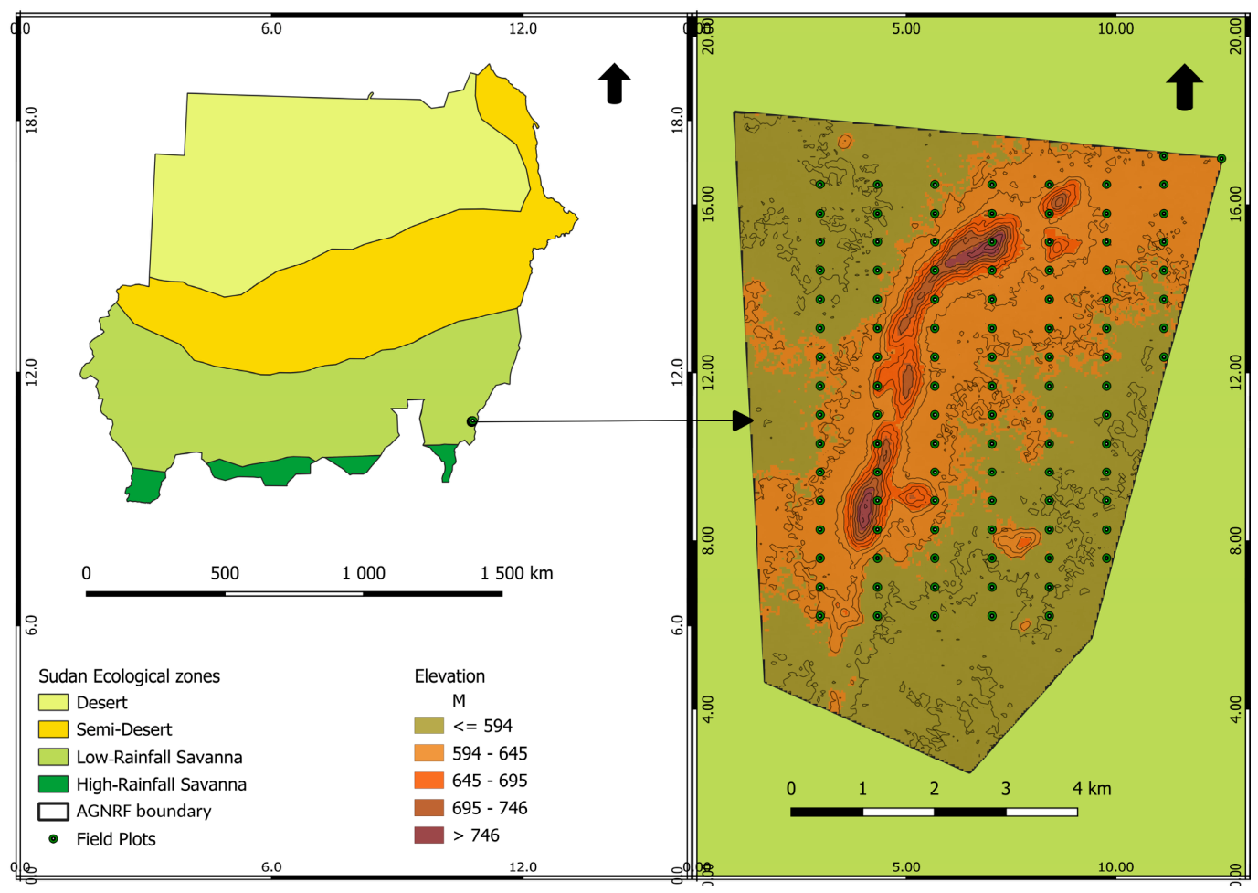
The study was conducted in the Abu-Gadaf Natural Reserved Forest (AGNRF), located within the Blue Nile Region (BNR), Sudan. It extends from 34.8486°E to 34.9110°E and 11.4188°N to 11.5021°N (WGS 84), with a centroid located at approximately 34.88°E, 11.46°N, covering approximately 4413.87 ha (Figure 1). The forest is characterized by a highly diverse woody vegetation community comprising fruit-bearing species alongside economically important gum-producing species including Acacia senegal, Acacia seyal, Boswellia papyrifera, and Commiphora africana, as well as multipurpose species locally utilized for medicine, fodder, construction, and fuelwood [20].

Topographically, the AGNRF exhibits strong heterogeneity, with mountainous terrain dominating the central sectors and flat to semi-flat landscapes prevailing in the forest edges. The climate is characterized by pronounced seasonality, with mean monthly rainfall ranging from less than 10 mm during the dry season (November–April) to over 270 mm in August, and mean temperatures ranging from approximately 23 °C in August to a maximum of 44 °C in March. Anthropogenic pressures are concentrated in flat peripheral areas, where proximity to human settlements drives livestock grazing, subsistence agriculture, and fuelwood extraction [20].

A systematic field campaign was conducted in January 2026 to quantify forest structure and support biomass modeling. A total of 103 rectangular sample plots (25 m × 40 m; 1000 m² each) were established using a grid-based design to ensure spatial representativeness across environmental gradients. Within each plot, all tree individuals were identified to species level and classified into developmental stages: adults (diameter at breast height (DBH) ≥ 7 cm), saplings (3 cm ≤ diameter < 7 cm), and seedlings (diameter < 3 cm). Structural attributes measured included DBH, total tree height, and crown diameter, using a diameter tape, Suunto clinometer, and Spiegel Relaskop, respectively.

2.2. Remote Sensing Data and Predictor Construction

Sentinel-2 Level-2A surface reflectance imagery was acquired for the 2025 growing season (June–October), corresponding to peak vegetation activity [21]. Scenes were filtered to retain observations with less than 20% cloud cover (CLOUDY_PIXEL_PERCENTAGE < 20) and further refined using probabilistic cloud and snow masking (MSK_CLDPRB < 40%, MSK_SNWPRB < 20%). Spectral bands B1–B12 were scaled to surface reflectance (÷10,000). A per-pixel median composite was then generated from all Sentinel-2 Level-2A scenes intersecting the study domain between 1 June and 30 October 2025 that passed these filters (n = 6 scenes), reducing atmospheric noise and residual cloud contamination. Three vegetation indices were derived: Normalized Difference Vegetation Index (NDVI), Normalized Difference Moisture Index (NDMI), and Normalized Burn Ratio (NBR), capturing vegetation greenness, moisture status, and disturbance signals [22]. Tasseled Cap transformation was applied using Sentinel-2-adapted coefficients to generate brightness, greenness, and wetness components [23]. Sentinel-2 bands were retained at their native spatial resolutions within the composite: B2, B3, B4 and B8 at 10 m; B5, B6, B7, B8A, B11 and B12 at 20 m; and B1 and B9 at 60 m. No band was resampled to a finer resolution prior to index computation. Vegetation indices and Tasseled Cap components were computed directly from the native resolution composite, so expressions combining bands of differing resolution were resolved at the resolution of the analysis grid. All predictor extraction and map production were performed on a common 30 m grid matched to the SRTM digital elevation model: bands finer than 30 m were aggregated by averaging, and the two 60 m bands were upsampled by nearest neighbor. Every predictor was therefore evaluated at 30 m regardless of its native resolution. Sentinel-1 C-band SAR data (VV and VH polarizations) were acquired for 2023 and processed in Interferometric Wide (IW) mode using median compositing. We acknowledge a temporal mismatch between the 2023 Sentinel-1 imagery and the 2025 Sentinel-2 composite. A 2025 Sentinel-1 composite temporally matched to Sentinel-2 was not feasible because 2025 IW acquisitions over the AGNRF had incomplete spatial coverage and elevated speckle due to gaps in orbital revisit and processing availability. Instead, we deliberately use the 2023 archive as a pragmatic trade-off. SAR backscatter and GLCM texture respond primarily to woody structural attributes (branch/stem density and canopy volume) that evolve gradually in savanna woodlands; over this ~2-year offset (2023 vs. 2025), we expect structural drift to contribute less to overall model error (RMSE ≈ 9 Mg ha⁻¹) than the biases that would arise from interpolating or gap filling a degraded 2025 dataset. We explicitly treat this temporal mismatch as a residual uncertainty source in Section 4.6. Derived predictors included VV and VH backscatter and the VH/VV ratio. Second-order texture metrics were computed using the Gray-Level Co-occurrence Matrix (GLCM) with a 5 × 5 kernel, extracting entropy and contrast for both VV and VH channels to capture spatial heterogeneity in canopy structure [24,25].

Topographic variables (elevation and slope) were derived from the SRTM digital elevation model at 30 m resolution to account for terrain-driven variability in biomass distribution [10]. Two Dynamic World predictors were derived from the 2025 annual modal class: a binary mask (dw) taking the value 1 for tree-dominated and shrub/scrub classes and 0 otherwise, and the modal class code itself (dw_label). Three classes occur among the training samples, trees, shrub and scrub, and crops with water and bare present elsewhere in the modeling domain. As dw_label is a nominal variable treated as numeric by the classifiers, its ordering carries no ecological meaning [26].

All variables were integrated into a multi-band predictor stack at 30 m spatial resolution, combining spectral, structural, and environmental information to characterize aboveground biomass variability (

Table 1. Summary of predictor variables used for AGB modeling.

Data Source	Group	Features	Description
Sentinel-2	Reflectance	B1 − B12	Surface reflectance across visible, red-edge, NIR, and SWIR wavelengths used to capture spectral properties of vegetation, soil, and moisture [27]
	Vegetation indices	NDVI (B8 − B4)/(B8 + B4)	Indicator of vegetation greenness and photosynthetic activity [28]
		NDMI (B8 − B11)/(B8 + B11)	Indicator of vegetation moisture content and water stress [29]
		NBR (NIR − SWIR2)/(NIR + SWIR2)	Sensitive to vegetation disturbance, burn severity, and canopy moisture [30]
	Tasseled Cap [31]	Brightness: B2, B3, B4, B8 + B11 and B12	Represents the overall reflectance of the land surface, mainly driven by soil and bare ground
		Greenness: B2, B3, B4, B8 + B11 and B12	Represents the vegetation component, specifically photosynthetic activity and vegetation vigor
		Wetness B2, B3, B4, B8 + B11 and B12	Represents moisture content in soil and vegetation, including surface water influence
Sentinel-1	Backscatter (SAR)	VV	Sensitive to surface roughness and vertical vegetation structure [9]
		VH	Sensitive to volume scattering from vegetation canopy [9]
		VH/VV	Ratio enhancing vegetation structure and moisture differences [9]
	Texture (SAR)	GLCM Entropy (VV, VH)	Measures spatial randomness and landscape heterogeneity [32]
		GLCM Contrast (VV, VH)	Measures local intensity variation and structural contrast [32]
SRTM–DEM	Topography	Elevation	Represents terrain-driven environmental gradients [33]
		Slope	Influences water flow, erosion, and vegetation distribution [33]
Dynamic World	Land cover	Dynamic World classes	Used for land cover stratification and masking of different surface types [26]

). All data processing was conducted within Google Earth Engine (GEE) platform (Google LLC, Mountain View, CA, USA; https://earthengine.google.com/, accessed on 26 March 2026). Allometric estimation and statistical analysis were performed in R version 4.3.2 (R Core Team, Vienna, Austria), and cartographic outputs were produced in QGIS version 3.34.11 (QGIS Association).

2.3. AGB Reference Data and Allometric Estimation

Plot-level AGB was derived from in situ measurements collected in January 2026. Plots with missing structural attributes were excluded prior to analysis. Tree-level AGB was estimated using the generalized pantropical allometric model of [34]

AGB = 0.0673 × (ρ × DBH² × H)^0.976

where AGB is aboveground biomass (kg), ρ is wood density (g cm⁻³), DBH is diameter at breast height (cm), and H is total tree height (m). Wood density values were obtained from the Global Wood Density Database via the BIOMASS R package (version 2.2.4.1) [35], applying species-level values where available and genus-level averages otherwise. Plot-level biomass was obtained by summing individual tree AGB values and converting to a per-hectare basis (Mg ha⁻¹). This model is fundamentally driven by woody structure and is insensitive to foliage presence, so the January dry-season campaign does not bias estimates despite possible deciduous leaf-off conditions.

To improve spatial representativeness, GEDI Level 4A footprint-level biomass estimates were used to augment the response variable. We state this explicitly to avoid ambiguity: GEDI observations were treated as additional measurements of AGB alongside the field plots, and no GEDI-derived quantity was included as an explanatory variable. The 29-band predictor stack described in Section 2.2 contains no GEDI input, and none of the variables in the importance analysis (Section 3.3) originates from GEDI. We used the LARSE/GEDI/GEDI04_A_002_MONTHLY product (L4A v2.1), comprising monthly granules intersecting the study domain and spanning (2019–2025). GEDI observations were filtered to retain high-quality estimates (0 < AGBD < 60 Mg ha⁻¹; standard error < 20 Mg ha⁻¹), resulting in 133 additional samples. To compensate for the very limited number of GEDI L4A footprints within the AGNRF boundary, the sampling domain was expanded to a 50 km buffer around the reserve. This approach is consistent with GEDI-based biomass workflows, which treat GEDI observations as spatially incomplete samples and often augment sparse local coverage by calibrating models with nearby observations and ancillary EO predictors [36,37]. The buffer was intended to increase the number of quality-filtered footprints while retaining vegetation and environmental conditions broadly representative of the reserve, an important consideration because GEDI model performance depends on training data spanning the range of conditions in the target domain [38]. After filtering, 56 GEDI footprints were retained within the 50 km buffer, although only one occurred inside the reserve itself, indicating that an in-reserve-only strategy would have provided an inadequate calibration sample. Expanding the sampling window therefore increased the size of the LiDAR reference dataset available for local biomass modeling, which is especially important in savanna and woodland systems where GEDI performance benefits from local or regionally adapted calibration [39]. The spatial distribution of all 56 GEDI footprints is visualized in Supplementary Figure S2. Whether the buffered domain is in fact representative of the reserve is a question we address directly in Section 2.6 and Section 3.5; the analyses reported there indicate that it is not, and this assumption should therefore be read as the design rationale adopted at the outset rather than as a property we were able to verify. A two-stage outlier filtering procedure was applied to the merged field and GEDI dataset. The initial dataset comprised 236 observations, including 103 field plots and 133 GEDI footprints. Following the removal of records with missing structural attributes or failed predictor extraction, 225 observations remained (94 field plots and 131 GEDI footprints). A subsequent two-stage filtering procedure was then applied. First, residual-based Z-scores were calculated from an initial Random Forest model fitted to the same dataset, and observations with |Z| > 2 were excluded. Second, samples with an Absolute Relative Error (ARE) greater than 50% were removed. This resulted in a final dataset of 100 observations, comprising 44 field plots and 56 GEDI footprints.

Field plots (25 m × 40 m; 1000 m²), GEDI footprints (approximately 25 m diameter) and the predictor grid (30 m) differ in spatial support. Predictor values were extracted at plot and footprint centroids as single-pixel samples rather than averaged over the plot or footprint area, and no correction was applied for GPS positional uncertainty. This simplification is a recognized limitation and is noted in Section 4.7. Retention rates were broadly similar between the two data sources, with 46.8% of field plots and 42.7% of GEDI footprints retained, corresponding to an overall retention of 44.4%. These comparable retention rates indicate that the filtering procedure did not disproportionately exclude one data source over the other. Nevertheless, more than half of the original observations (56%) were removed, reflecting the stringent filtering required to reduce noise and extreme prediction errors in this highly heterogeneous dry savanna ecosystem.

We emphasize that this filtering procedure is not statistically neutral with respect to model evaluation. Because the residual-based Z-score criterion was derived from an initial Random Forest model fitted to the same observations, samples that were poorly predicted by that model were more likely to be excluded. Consequently, model performance assessed on the retained dataset is expected to be more optimistic than performance on the complete, unfiltered dataset. We report this limitation explicitly rather than treating the filtered dataset as an unbiased sample and recommend that future studies applying similar filtering procedures report model accuracy for both filtered and unfiltered datasets. Together with the source heterogeneity discussed in Section 3.5, this filtering-induced bias suggests that the reported accuracy metrics should be interpreted as upper-bound estimates of model performance rather than fully independent validation statistics.

2.4. Multi-Model Machine Learning Framework

AGB was modeled using three machine learning algorithms: RF, GB, and CART, all implemented within GEE. These algorithms were selected for their ability to capture nonlinear relationships, accommodate high-dimensional predictor spaces, and maintain robustness under multicollinearity [14]. RF models were trained with 500 trees and a bagging fraction of 0.7 for all cross-validated and ensemble configurations; the split-sample validation model used 1000 trees. GB models used 500 trees, a shrinkage parameter of 0.1, and a sampling rate of 0.7 with a least-squares loss, consistent with GB settings commonly tuned to balance learning rate and subsampling in biomass applications [40,41]. CART models were constrained to a maximum of 20 terminal nodes with a minimum leaf population of 5 to reduce overfitting, in line with evidence that shallow, regularized trees generalize better than fully grown trees in AGB mapping [42]. These values were adopted from published biomass modeling applications and were not tuned on the present dataset; no hyperparameter search was conducted (Section 4.7).

All three algorithms were implemented using the SMILE library as exposed in Google Earth Engine (smileRandomForest, smileGradientTreeBoost and smileCart), and variable importance was obtained in every case from the trained classifier’s explain () method, which returns mean decrease in impurity. For each predictor, this is the total reduction in node variance attributable to splits on that predictor, summed across all splits in which it appears and accumulated over the trees comprising the model: 1000 trees for the Random Forest model from which importance was extracted, 500 for Gradient Boosting, and a single tree for CART. The estimation mechanism is therefore identical across the three architectures and differs only in the number of trees over which the reduction is accumulated, which makes the relative rankings comparable in kind while their absolute magnitudes are not; importance values were accordingly normalized within each model before plotting (Section 3.3). Two properties of impurity-based importance bear on the interpretation of these rankings. It is biased toward predictors offering more distinct split points, and it divides credit arbitrarily among correlated predictors, so that one member of a correlated group may absorb importance that could equally have been attributed to another. Our predictor stack contains several strongly correlated groups, particularly among the Sentinel-2 bands, and the rankings reported in Section 3.3 should be read with this in mind. Permutation importance would be less susceptible to both effects but is not available for these classifiers within Earth Engine. Each algorithm was trained twice: once using the full predictor set (29 variables) and once using a reduced set of the top 15 predictors, identified through variable importance rankings derived from the respective full models. This yielded six model configurations (RF_full, RF_top15, GB_full, GB_top15, CART_full, CART_top15) for comparative evaluation. The top 15 predictor lists were derived independently for each algorithm, ensuring that the reduced model for each algorithm reflects its own internal importance structure rather than a single shared ranking.

Partial model uncertainty was quantified from two complementary perspectives: (i) within-algorithm ensemble variability, computed as the standard deviation of five independently seeded models per algorithm, providing a measure of stochastic variability within each approach; and (ii) cross-model disagreement, computed as the pixel-wise standard deviation of the three ensemble mean maps (RF, GB, CART), capturing structural uncertainty arising from algorithm choice. Final AGB maps were produced at 30 m spatial resolution using the reduced predictor sets for each algorithm.

Variable importance was computed once from models trained on the full training partition, and the resulting top 15 sets were held fixed across all cross-validation folds rather than re-derived within each fold.

2.5. Model Validation Strategy

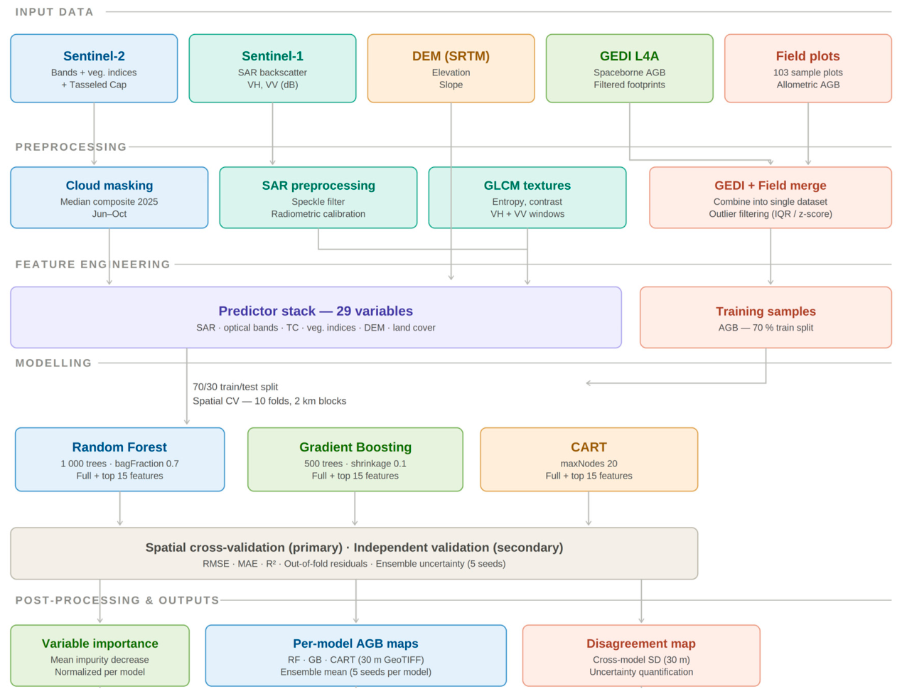
Model performance was evaluated using two complementary validation approaches. First, a random 70/30 split-sample validation was applied to assess in-sample predictive accuracy. Second, and serving as the primary evaluation framework, spatially explicit 10-fold block cross-validation was conducted. The 2 km block size was selected following a sensitivity analysis in which the 10-fold spatial cross-validation was repeated at block sizes of 1, 2, 3 and 5 km (Table S2). Model performance degraded monotonically with increasing block size, as expected under stricter geographic separation between training and test data. The interval from 1 to 2 km showed the smallest change in R² (−0.016 for RF, compared with −0.056 from 2 to 3 km), indicating that 2 km lies at the edge of the stable region of the sensitivity curve. Performance did not, however, reach a plateau within the tested range, implying that residual spatial dependence persists beyond 2 km and that the 5 km results (RF R² = 0.298) represent a more conservative bound. Grid blocks were allocated to folds in round-robin order; samples falling within a single block were therefore never divided between training and test sets, although adjacent blocks may be assigned to different folds. Because samples are distributed across the buffered modeling domain rather than densely within the reserve, increasing the block size from 1 to 5 km reduced the number of occupied blocks only from 84 to 57. This approach accounts for spatial autocorrelation and provides a more realistic estimate of model generalization performance across unseen areas [43]. Performance metrics included Root Mean Squared Error (RMSE), Mean Absolute Error (MAE), and the coefficient of determination (R²). The workflow is summarized in Figure 2.

2.6. Assessment of Reference Data Heterogeneity

Because the field and GEDI reference samples were drawn from different spatial domains (Section 2.2 and Section 2.3), we tested whether they could be treated as a single homogeneous training population and quantified the consequences of any heterogeneity for model evaluation. Five analyses were performed.

First, distributional homogeneity was assessed using a two-sample Kolmogorov–Smirnov test on field-measured and GEDI-derived AGB, complemented by a Mann–Whitney U test as a rank-based alternative robust to differences in distributional shape.

Second, spatial cross-validation was performed separately on the field-only subset (n = 44), the GEDI-only subset (n = 56) and the merged dataset (n = 100), using identical predictors and fold structure. Ten folds were used for all three arms, consistent with the primary validation design described in Section 2.5. We note that the field-only subset of 44 samples yields approximately four observations per test fold, so per-fold estimates in that arm are correspondingly unstable; the near-zero field-only and within-field coefficients reported in Section 3.5 are consistent across all three algorithms and across both five-fold and ten-fold configurations, which is the basis on which we interpret them.

Third, out-of-fold predictions from the merged models were decomposed by data source, and R² and RMSE were recomputed separately within the field and GEDI populations. If a model predicts AGB from vegetation structure, skill should be evident within each population; if it instead exploits the difference between them, skill will appear only in the pooled statistics.

Fourth, the separability of the two sources was tested directly by training a Random Forest classifier to predict data source from the 29-band predictor stack alone, with AGB excluded. Out-of-fold classification accuracy was compared against the majority-class baseline of 0.56.

Fifth, a quantile-mapping calibration was derived by regressing paired percentiles (5th to 95th, in 5% increments) of the field distribution on those of the GEDI distribution, and the merged spatial cross-validation was repeated using the calibrated values. We emphasize that this procedure aligns marginal distributions and does not constitute a validated sensor bias correction, since the absence of co-located field and GEDI observations prevents direct calibration. As a further check, the merged analysis was repeated with GEDI footprints restricted to within 5, 10 and 20 km of the reserve boundary.

3. Results

3.1. Spatial Distribution of Aboveground Biomass

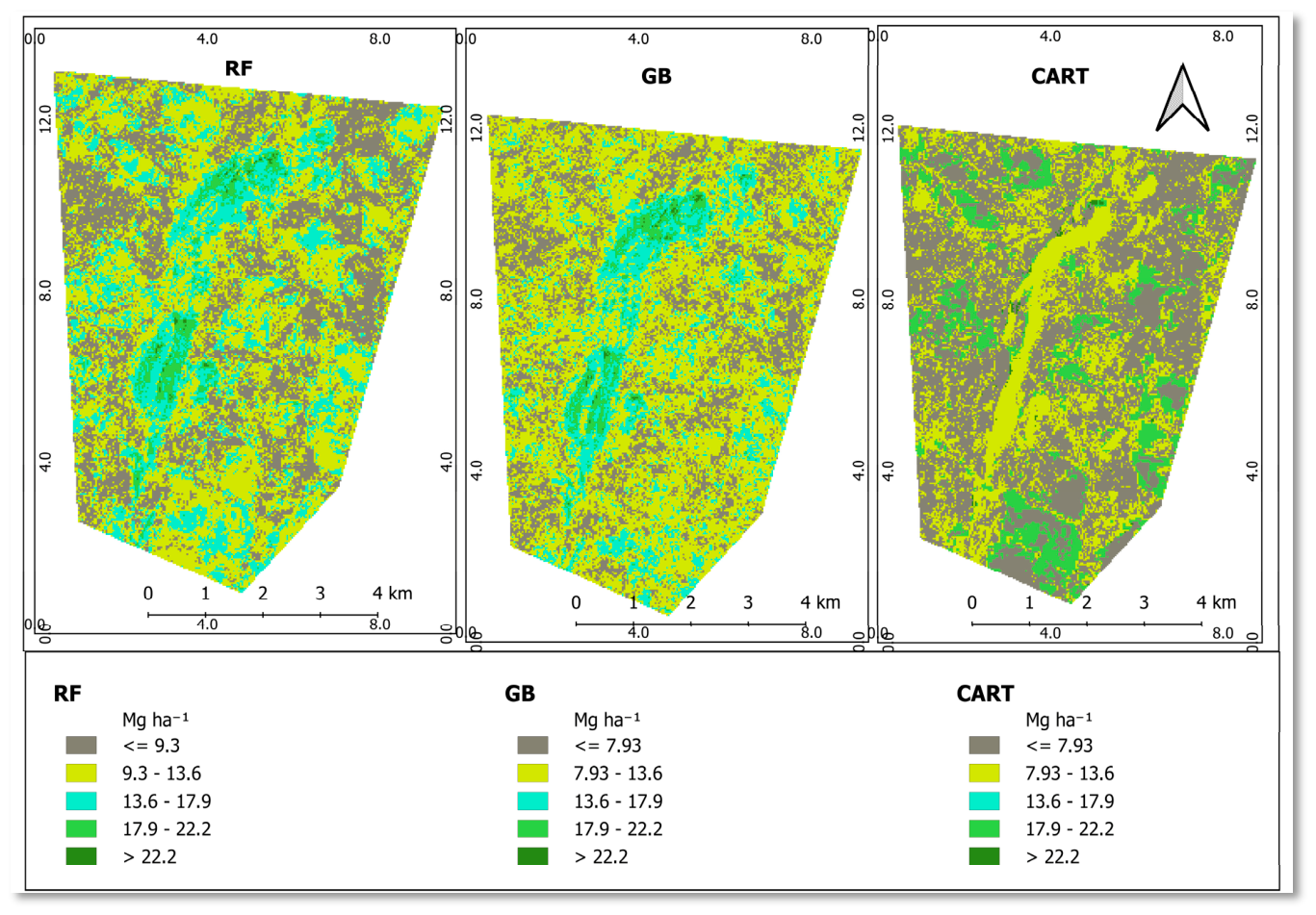
The following describes the relative spatial distribution of predicted AGB across the AGNRF. As established in Section 3.5, the absolute values cannot be treated as validated biomass estimates; the patterns below should therefore be interpreted as indicating where models predict higher or lower biomass relative to one another, rather than as quantified stocks. The predicted AGB exhibited clear spatial heterogeneity across the AGNRF, with differences in value ranges among the three models (Figure 3). The RF model estimated AGB values ranging from 5.01 to 26.56 Mg ha⁻¹, while the GB model showed a wider range from 0.32 to 38.36 Mg ha⁻¹. The CART model produced values ranging from 3.70 to 36.77 Mg ha⁻¹.

Both RF and GB revealed similar spatial patterns, characterized by a pronounced central biomass corridor forming a continuous strip extending from the northern to the southern parts of the reserve. This zone represented the highest biomass concentrations within the study area. A spatial correspondence between AGB distribution and topographic variation was observed in the RF and GB outputs, where higher biomass values were associated with higher elevation areas, while lower biomass values were found in lower elevation zones. Low biomass values were also predominantly concentrated along the forest edges, forming a boundary of reduced biomass surrounding the core forest area. In contrast, the CART model showed a different spatial pattern. Low biomass values dominated most of the landscape, while higher biomass values were distributed in scattered patches around the forest without a clear spatial structure.

Pairwise correlation of ensemble means AGB predictions revealed strong agreement between RF and GB (Pearson r = 0.86, Spearman ρ = 0.84), indicating broadly consistent spatial patterns between the two ensemble-based models. Agreement between RF and CART was moderate (Pearson r = 0.52, Spearman ρ = 0.61), while GB and CART showed the weakest correspondence (Pearson r = 0.36, Spearman ρ = 0.44) (

Table 2. Pearson (r) and Spearman (ρ) correlation coefficients of pixel-level ensemble mean AGB predictions between RF, GB and CART, computed over all 30 m pixels within the AGNRF boundary (n = 49,043). Values on the diagonal equal 1.0 by definition.

Model Pair	Pearson r	Spearman ρ
RF–GB	0.859	0.838
RF–CART	0.520	0.608
GB–CART	0.357	0.443

), suggesting that CART predicts a substantially different spatial distribution of biomass relative to the other two models. The consistent divergence between Pearson and Spearman values particularly for GB–CART indicates that model disagreement is concentrated at the upper tail of the AGB distribution, where high-biomass areas are predicted most differently across algorithms.

3.2. Model Performance

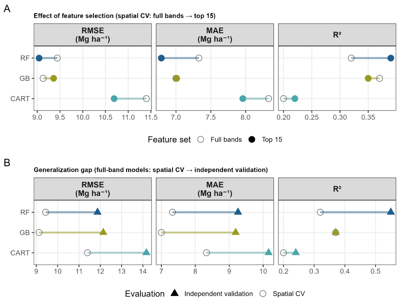
Model performance varied considerably across algorithms and validation strategies, underscoring the critical role of evaluation approach in biomass modeling accuracy. Under spatial cross-validation (2 km block CV), the RF model with all predictors achieved an RMSE of 9.44 Mg ha⁻¹, MAE of 7.33 Mg ha⁻¹, and R² of 0.32. Feature selection initially appeared to improve RF performance under spatial cross-validation (RMSE 9.44 to 9.04 Mg ha⁻¹; R² 0.32 to 0.39). Because predictor selection was performed once on the full training partition rather than within each fold, we tested whether this improvement survived a nested procedure in which the top 15 predictors were re-derived from the training portion of each fold. It did not; nested selection returned an RMSE 9.40 Mg ha⁻¹ and R² 0.33, effectively identical to the full 29-band model (9.40, 0.33). The apparent benefit of feature reduction was therefore an artefact of selecting predictors on data subsequently used for testing. We report full-band results as primary throughout, and no configuration is advanced as best-performing.

The GB model with all predictors performed comparably to RF with all predictors under spatial CV, with an RMSE of 9.13 Mg ha⁻¹, MAE of 7.00 Mg ha⁻¹, and R² of 0.37. Notably, feature selection did not yield improvement for GB: the reduced model (top15), which produced a slightly higher RMSE of 9.36 Mg ha⁻¹ and a lower R² of 0.35, suggesting that GB is less sensitive to predictor reduction and may rely on a broader feature set to capture nonlinear biomass gradients.

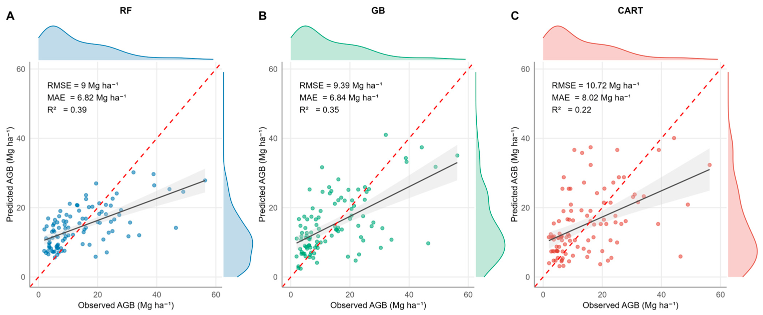
The CART model showed the weakest spatial CV performance across both configurations. All predictors yielded an RMSE of 11.40 Mg ha⁻¹, MAE of 8.33 Mg ha⁻¹, and R² of 0.20, while the reduced version (top 15) offered a modest improvement (RMSE = 10.69 Mg ha⁻¹, R² = 0.22), consistent with its inherent tendency toward overfitting and poor generalization across spatial gradients (Figure 4).

Under the random 70/30 split-sample validation, all models returned higher RMSE values than under spatial cross-validation: RF 11.87 against 9.44 Mg ha⁻¹, GB 12.14 against 9.13, and CART 14.16 against 11.40. The R² pattern differed. RF returned a substantially higher R² under the random split (0.55 against 0.32), GB an almost identical value (0.3702 against 0.3704), and CART a marginally higher one (0.24 against 0.20).

These two metrics therefore point in opposite directions, and the comparison requires more caution than a simple inflation narrative allows. Two factors complicate it. First, the two designs differ in training set size: 10-fold spatial cross-validation trains each model on approximately 90 samples, whereas the 70/30 split trains on 78, so a higher RMSE under the random split is expected on sample size grounds alone. Second, R² depends on the variance in the evaluation set, and the random holdout comprises only 22 samples, making both metrics unstable and not directly comparable across designs. We therefore conclude only that RF showed a markedly higher R² under random validation, consistent with spatial autocorrelation inflating that particular statistic, and that this pattern was not reproduced by GB or CART. We do not claim a systematic inflation effect across algorithms or metrics.

The interpretation of all pooled statistics in this section is further qualified by the source decomposition analysis in Section 3.5. Observed versus predicted relationships (Figure 5) should be interpreted along two independent axes: dispersion about the fitted line, and departure of that line from the 1:1 relationship. The first reflects the strength of the observed–predicted association and is summarized by R²; the second reflects systematic bias and is not.

RF produced the least dispersed predictions, consistent with its higher R² (0.392), but its fitted slope of 0.317 departs furthest from unity of the three models. GB showed greater dispersion and a lower R² (0.346) but a fitted slope of 0.428, the closest to unity and therefore the smallest systematic bias. CART was intermediate in slope (0.378) while showing the greatest dispersion and the lowest R² (0.225). Expressed as angular departure from the 1:1 line, the values are 27.4° for RF, 24.3° for CART and 21.9° for GB. Precision and freedom from bias are thus inversely ordered between RF and GB, and no single model performs best on both criteria.

All three fitted lines have slopes well below unity and positive intercepts (9.8–11.0 Mg ha⁻¹), intersecting the 1:1 line between approximately 16 and 17 Mg ha⁻¹. Predictions are consequently compressed toward the conditional mean, over-predicting at low observed AGB and under-predicting at high values. The drivers of this compression are examined in Section 4.1.

The 10-fold spatial cross-validation revealed substantial heterogeneity in model performance across geographical blocks. RF achieved the lowest RMSE in fold 6 (4.27 Mg ha⁻¹) but the highest in fold 1 (9.92 Mg ha⁻¹), while GB showed more balanced fold-to-fold results (RMSE range 5.54–11.06 Mg ha⁻¹). For GB, R² values were 0.3704 under spatial cross-validation and 0.3702 under the random split; the apparent equality in Figure 4B is due to rounding to three decimal places. The complete per-fold metrics are presented in Supplementary Material Table S1.

3.3. Variable Importance

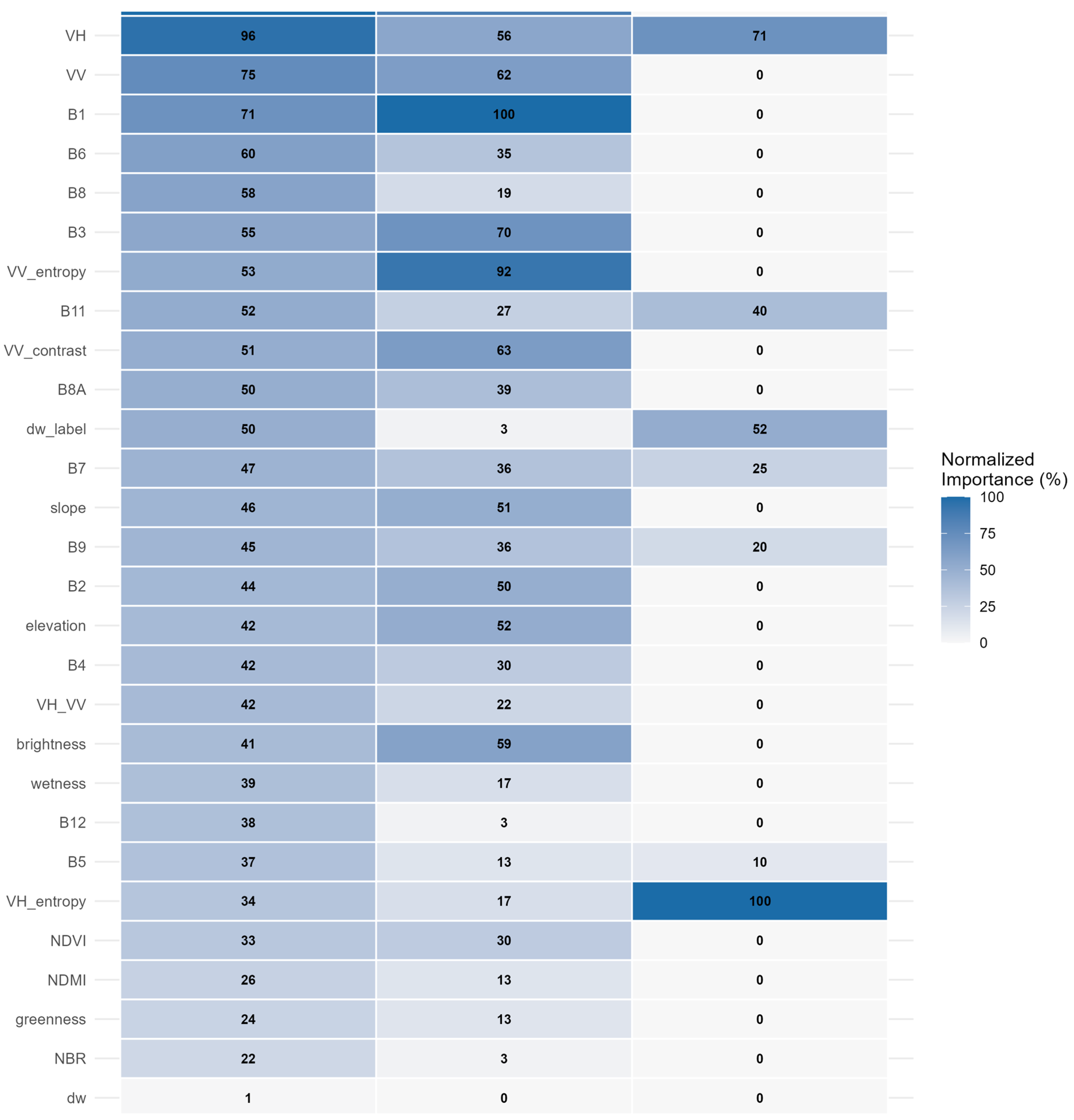
Analysis of variable importance revealed consistent patterns across RF and GB models, with SAR-derived variables dominating the upper ranks, while CART showed a markedly different and more sparse importance distribution (Figure 6).

In the RF model, VH_contrast emerged as the single most important predictor, followed closely by VH backscatter and VV backscatter. This pattern confirms that SAR-derived structural texture and radar backscatter intensity are the primary drivers of AGB prediction, reflecting their sensitivity to canopy density and woody biomass. Among optical predictors, Sentinel-2 bands B1, B3, B6, B8, and B11 contributed substantially, capturing vegetation reflectance across visible, red-edge, and shortwave infrared wavelengths. VV_entropy and VV_contrast further reinforced the dominance of SAR texture metrics in explaining biomass variability. Vegetation indices (NDVI, NDMI, NBR) and topographic variables (elevation, slope) ranked in the middle tier, while the Dynamic World variable (dw) recorded the lowest importance score.

The GB model exhibited a broadly consistent ranking with RF. VV_entropy and VH_contrast ranked as the two most important predictors, alongside brightness (a Tasseled Cap component) and topographic variables, which featured more prominently in GB than in RF. Optical bands contributed moderately, with B1 and B8A among the highest-ranked spectral predictors. The Dynamic World variable recorded zero importance in GB, indicating no contribution to model splits.

The CART model showed a substantially different importance profile, with importance concentrated in very few predictors and zero scores assigned to the majority of variables. VH_entropy was the most important predictor by a considerable margin, followed by VH backscatter and the Dynamic World label. Elevation, slope, greenness, wetness, and all vegetation indices contributed nothing to CART splits, reflecting the model’s limited capacity to leverage multi-source predictor diversity. Across all three models, SAR-derived variables consistently emerged as the most informative predictors, underscoring the added value of integrating radar data with optical and topographic information in dryland biomass modeling frameworks.

3.4. Uncertainty Analysis

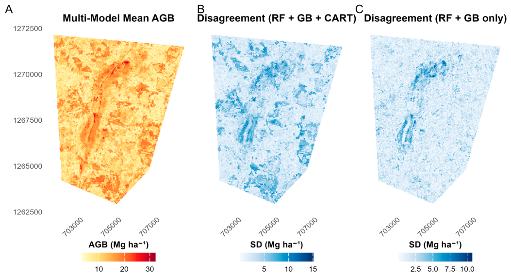
Within-algorithm ensemble uncertainty varied substantially across the three models (Figure 7A). The RF ensemble exhibited low variability (SD range: 0.01–0.99 Mg ha⁻¹; mean = 0.28 Mg ha⁻¹), with higher uncertainty (>0.6 Mg ha⁻¹) concentrated in the central high-biomass corridor and lower values (<0.1 Mg ha⁻¹) in low-biomass peripheral areas (Figure S1A). The GB ensemble showed considerably higher uncertainty (range: 0.08–5.53 Mg ha⁻¹; mean = 1.63 Mg ha⁻¹), distributed widely across the forest interior without a consistent spatial gradient (Figure S1B). The CART ensemble produced a constant standard deviation of zero throughout the study area (Figure S1C), which is an expected result given that CART is a deterministic algorithm: identical training data and parameters yield identical trees with no stochastic variation. CART was excluded from the within-algorithm ensemble variability analysis, since as a deterministic algorithm, it yields identical trees across seeds and a standard deviation of exactly zero, which would be misinterpreted as high confidence. It was retained in the multi-model mean and cross-model disagreement analyses, since excluding a model on grounds of poor performance would restrict the ensemble to members selected for their agreement and would understate structural uncertainty by construction. We therefore report disagreement across all three algorithms (Figure 7B) and, separately, across RF and GB alone (Figure 7C), so that CART’s contribution to the total spread is explicit rather than removed. It was retained in the cross-model disagreement analysis, where its ensemble mean contributes as one of three model outputs. Cross-model disagreement, expressed as the pixel-wise standard deviation of the three ensemble mean maps (RF, GB, CART), ranged from 0.03 to 15.12 Mg ha⁻¹ across the study area, with a mean of 3.33 Mg ha⁻¹ and a median of 2.63 Mg ha⁻¹ (Figure 7B). High disagreement (>5 Mg ha⁻¹) occurred on approximately 7.4% of forested pixels, predominantly in the central high-biomass corridor and along rugged terrain where structural complexity amplifies algorithm-specific responses. Low disagreement (<2 Mg ha⁻¹) prevailed in low-biomass peripheral areas, where all three algorithms converged on similar predictions.

To isolate the uncertainty arising exclusively from the RF and GB algorithms, we additionally calculated cross-model disagreement excluding CART (Figure 7C). The RF–GB disagreement ranged from ~1 to ~10 Mg ha⁻¹, with a substantially lower mean and median compared to the three-model metric. Critically, the extreme disagreement hotspots exceeding 10 Mg ha⁻¹ observed in Figure 7B were absent in the RF–GB comparison; instead, the highest RF–GB divergence (6–10 Mg ha⁻¹) appeared as more spatially confined patches, primarily along the margins of the central high-biomass corridor rather than throughout its core. This pattern confirms that CART’s divergent predictions, not structural differences between RF and GB, were the primary driver of the elevated disagreement in the central corridor. The RF–GB disagreement remained modest across most of the forest interior, suggesting that the two ensemble methods provide broadly consistent spatial predictions when the poorly performing CART is excluded.

Together, the two uncertainty metrics reveal that: (i) within-algorithm uncertainty is low for RF (mean 0.28 Mg ha⁻¹) but substantially higher for GB (1.63 Mg ha⁻¹); (ii) cross-algorithm disagreement including all three models is modest on average (mean 3.33 Mg ha⁻¹) but locally exceeds 15 Mg ha⁻¹ in structurally heterogeneous zones (Figure 7B); and (iii) this local extreme disagreement is almost entirely driven by CART, as RF and GB show much closer agreement when compared directly (Figure 7C), with a maximum divergence of approximately 10 Mg ha⁻¹ confined to small patches near the high-biomass corridor. These metrics describe the sensitivity of the predicted surface to algorithm choice; they do not constitute an estimate of prediction error. Each contributing map carries its own error and residual spatial dependence, which are not separable once the outputs are averaged, and we therefore draw no conclusion about how an operational ensemble should be weighted. Establishing whether any weighting scheme improves predictive performance would require independent validation of the ensemble itself, which the present data do not support.

3.5. Reference Data Heterogeneity and Its Effect on Apparent Accuracy

Field-measured and GEDI-derived AGB differed substantially in both level and spread. Field plots (n = 44) had a mean AGB of 8.89 Mg ha⁻¹ (median 6.45, SD 6.60, range 1.95–30.42), whereas GEDI footprints (n = 56) had a mean of 18.71 Mg ha⁻¹ (median 16.57, SD 12.48, range 2.01–56.30), a factor of 2.1 higher. A two-sample Kolmogorov–Smirnov test rejected the null hypothesis of a common distribution (D = 0.531; 5% critical value 0.274; p ≈ 8 × 10⁻⁷), as did a Mann–Whitney U test (U = 586, z = −4.49, p < 0.001).

Models trained on the merged dataset substantially outperformed those trained on field plots alone (

Table 3. Spatial cross-validation performance by training dataset and by source (10-fold, 2 km blocks, full 29-band predictor set).

Training Data	Model	RMSE	MAE	R2 Pooled	R2 Within-Field	R2 Within-GEDI
Field only (n = 44)	RF	6.58	4.67	0.065	—	—
Field only (n = 44)	GB	7.91	5.93	0.004	—	—
Field only (n = 44)	CART	7.16	4.81	0.054	—	—
GEDI only (n = 56)	RF	11.38	9.13	0.172	—	—
GEDI only (n = 56)	GB	11.01	9.06	0.254	—	—
GEDI only (n = 56)	CART	14.13	11.83	0.059	—	—
Merged (n = 100)	RF	9.40	7.34	0.331	0.023	0.276
Merged (n = 100)	GB	9.45	7.32	0.331	0.006	0.306
Merged (n = 100)	CART	11.40	8.33	0.202	0.001	0.184
Merged, calibrated	RF	5.90	4.34	0.128	—	—
Merged, calibrated	GB	6.22	4.74	0.101	—	—
Merged, calibrated	CART	6.86	5.31	0.063	—	—

). Random Forest R² rose from 0.065 to 0.331, Gradient Boosting from 0.004 to 0.331, and CART from 0.054 to 0.202. Interpreted conventionally, this would indicate a large benefit from GEDI fusion.

Decomposing the merged models’ out-of-fold predictions by source shows that this interpretation is not supported. Within the field plot population, predictive skill was effectively absent: R² was 0.023 for RF, 0.006 for GB and 0.001 for CART. Within the GEDI population, it was appreciably higher (0.276, 0.306 and 0.184 respectively), but no model achieved meaningful skill in the population that constitutes the ground-based reference for the reserve interior. The models also reproduced the between-source level difference closely: RF predicted mean values of 10.67 Mg ha⁻¹ for field samples and 17.49 for GEDI samples, against observed means of 8.89 and 18.71.

Three further analyses confirm that the pooled performance reflects separation between the two reference populations. A Random Forest trained to classify data source from the predictor stack alone, with AGB excluded, achieved 85% out-of-fold accuracy against a 56% majority-class baseline, demonstrating that the predictors encode the spatial domain from which a sample originates. Quantile calibration that aligned the two distributions (slope 0.4875, offset −0.290, bringing the GEDI mean to 8.83 against a field mean of 8.89) reduced pooled RF R² from 0.331 to 0.128, indicating that approximately three-fifths of the apparent skill was attributable to the inter-source level difference. Finally, GEDI-derived AGB increased with distance from the reserve, averaging 21.2 Mg ha⁻¹ beyond 20 km compared with approximately 13 Mg ha⁻¹ within 20 km; progressively restricting GEDI footprints to the vicinity of the reserve reduced merged RF R² to 0.080 (within 5 km), 0.038 (within 10 km) and 0.008 (within 20 km, n = 61).

Fusion did confer one measurable benefit. Training on the merged dataset improved prediction of GEDI-derived AGB relative to training on GEDI alone, with within-GEDI R² rising from 0.172 to 0.276 for RF, from 0.254 to 0.306 for GB, and from 0.059 to 0.184 for CART. The field plots therefore contribute information useful for predicting GEDI’s own biomass estimates. This does not, however, constitute evidence of accuracy against ground-measured biomass, which is the quantity of interest for the reserve.

Taken together, these results indicate that the apparent accuracy of the fused models arises predominantly from discrimination between two dissimilar reference populations rather than from prediction of AGB from vegetation structure. Critically, spatially explicit block cross-validation did not reveal this: it enforces geographic separation between training and test samples but does not test whether those samples belong to a common population.

4. Discussion

4.1. Model Performance and Algorithm Comparison

The multi-model comparison must be interpreted in light of the reference data heterogeneity documented in Section 3.5. On the merged dataset, RF and GB achieved effectively identical pooled performance (R² = 0.331 for both) and both exceeded CART (0.202), a ranking consistent with the general expectation that ensemble methods outperform single trees [14]. However, because the pooled statistics are substantially driven by separation between the field and GEDI populations, this ranking primarily reflects how efficiently each algorithm exploits that contrast rather than differences in their capacity to predict biomass from vegetation structure. The within-field decomposition supports this reading: no algorithm achieved meaningful skill in that population (R² = 0.001–0.023), and the ordering among them is not stable at those magnitudes. The structural distinction between the algorithms nevertheless remains visible in their variable importance profiles: CART deterministically selects one best split per node, concentrating predictive credit in a small subset of correlated bands, whereas RF and GB distribute it across hundreds of trees through subsampling and averaging (Figure 6; see also [44]). This explains why CART assigned zero importance to the majority of predictors, including all vegetation indices and topographic variables. Within the GEDI population, where sample size is larger and the AGB range wider, differences between algorithms are more interpretable. GB achieved the highest within-GEDI R² (0.306), followed by RF (0.276) and CART (0.184), and GB also outperformed the other algorithms when trained on GEDI data alone (R² = 0.254 against 0.172 for RF and 0.059 for CART). This is consistent with the sequential error correction mechanism of boosting being advantageous where the target variable has substantial spread. We note, however, that GEDI-only performance itself is modest, and that the relationship being learned is between the predictor stack and GEDI’s own model-derived AGB estimates rather than field-measured biomass [12,45].

The relationship between validation design and reported accuracy is less straightforward than our original analysis suggested. RF returned a substantially higher R² under random splitting than under spatial cross-validation (0.55 against 0.32), consistent with the well-documented effect of spatial autocorrelation inflating apparent accuracy when training and test samples are drawn from similar geographic neighborhoods [43]. This pattern was not, however, general: GB returned effectively unchanged values (0.3704 under spatial cross-validation against 0.3702 under the random split), CART differed only marginally (0.24 against 0.20), and RMSE was higher under the random split for all three models, which is the opposite of what accuracy inflation would predict. Part of this discrepancy is attributable to design rather than to spatial structure, since the random split trains on fewer samples than 10-fold cross-validation and evaluates only 22 observations. We therefore report the RF result as consistent with the findings of [16,18] in West African and pantropical settings, while declining to generalize it across algorithms or metrics from our data. Spatial cross-validation nevertheless remains the more conservative design in principle, and our results identify a further limitation of it. Because it enforces geographic separation without testing whether training and test samples belong to a common population, it did not detect the source heterogeneity that accounts for most of the apparent accuracy reported here (Section 3.5). Spatial cross-validation should thus be regarded as necessary but not sufficient where reference data are fused from heterogeneous sources.

A systematic conditional bias is also evident in Figure 5, where all three algorithms progressively underestimate observed AGB as values increase beyond approximately 40 Mg ha⁻¹. The bias is most pronounced at the highest observed values, which reach 56.3 Mg ha⁻¹. Four compounding constraints contribute to this pattern. First, the final training set of 100 samples contains few high-AGB instances, causing tree-based methods to regress toward the conditional mean, a classical shrinkage effect amplified when the response variable is unbalanced [40]. Second, the quality filter applied to GEDI L4A data (retaining only 0 < AGBD < 60 Mg ha⁻¹) truncated the upper tail of the spaceborne LiDAR contribution, removing precisely the high-biomass examples that could have informed upper-tail predictions. Third, Sentinel-1 C-band backscatter approaches saturation at relatively low biomass levels, typically in the range of 20–50 Mg ha⁻¹, which falls within rather than above the range observed here, and Sentinel-2 reflectance saturates as canopy closure increases; discriminative power is therefore reduced across much of the upper portion of our observed distribution [16]. Fourth, the field reference AGB itself, derived from the pantropical allometric model of Chave et al. (2014) [34], carries calibration uncertainty that is largest for large-diameter trees, implying that part of the apparent under-prediction may originate in the reference data rather than in the algorithms. A fifth consideration follows from Section 3.5: because the upper tail of the pooled AGB distribution is composed almost entirely of GEDI observations (field values reach 30.4 Mg ha⁻¹ against 56.3 for GEDI), the apparent underestimation at high biomass is predominantly underestimation of high GEDI values and is therefore not independent of the source heterogeneity described above.

4.2. Implications for Field and Spaceborne LiDAR Reference Fusion

Supplementing sparse field plots with GEDI footprint estimates is now common practice in data-scarce regions and is generally reported to improve model performance [16]. Our results indicate that where the two sources occupy different spatial domains, such improvement may be partly or largely artefactual. The mechanism is straightforward: when field and LiDAR samples are drawn from areas differing systematically in biomass, and the predictor stack encodes the environmental characteristics distinguishing those areas, a flexible learner can achieve substantial apparent accuracy simply by identifying which population a sample belongs to. The model then appears skillful in pooled evaluation while resolving little biomass variation within the population of interest. Here, the predictors permitted source classification at 85% accuracy against a 56% baseline, and removing the inter-source level difference eliminated approximately three-fifths of the apparent skill.

The most consequential implication concerns validation practice. Spatially explicit cross-validation is now widely and correctly advocated as a corrective to accuracy inflation from spatial autocorrelation [18], but it does not address this second and distinct problem. Block cross-validation enforces geographic separation between training and test samples; it does not test whether those samples originate from populations with comparable biomass distributions. In our design, the two are partially confounded, since field plots occupy the reserve while most GEDI footprints lie beyond it. A validation scheme conservative with respect to spatial autocorrelation may therefore remain permissive with respect to population heterogeneity. We suggest that studies fusing heterogeneous reference data report three inexpensive diagnostics as a minimum: a formal test of distributional homogeneity between sources, performance decomposed by source rather than pooled, and comparison against models trained on each source independently.

That GEDI L4A substantially exceeds field-measured AGB in this sparse savanna system is consistent with previous evaluations. Li et al. (2024) [39] reported degraded GEDI footprint-level performance in Southern African savannas under precisely the structurally heterogeneous, low-biomass conditions prevailing at the AGNRF, and footprint-level uncertainty is known to be greatest in open canopies [45]. Whether the discrepancy reflects GEDI overestimation, a genuine biomass gradient between the reserve and its surroundings, or both cannot be resolved without co-located measurements; we identify this as a priority for future work.

4.3. Importance of Multi-Source Data Integration

The complementary nature of optical, SAR, and LiDAR data is clearly reflected in the variable importance results. SAR-derived texture metrics, particularly VH contrast and VV entropy, consistently ranked as the most important predictors across RF and GB, confirming that canopy structural heterogeneity captured by radar backscatter is the primary determinant of AGB variability in this dryland system. This aligns with findings from Tamga et al. (2022) [16], who demonstrated that combining Sentinel-1 and Sentinel-2 outperformed single-sensor approaches in AGB estimation across agroforestry systems (best R² = 0.91 for S1 + S2), and [46,47], who highlighted the essential structural information contributed by C-band SAR in tropical biomass estimation.

Optical indicators, including NDVI, greenness, and key Sentinel-2 bands, captured vegetation vigor, productivity, and biochemical properties [48], while topographic variables (elevation and slope) featured more prominently in GB than in RF, consistent with their role as surrogates for moisture availability and anthropogenic accessibility gradients. The integration of GEDI-derived AGB samples provided critical vertical structure information not detectable through optical or SAR data alone, significantly extending the spatial coverage of training data beyond the 103 field plots. This is consistent with [13,49], who showed that GEDI structural metrics dramatically improved footprint-level AGB predictions compared to single-sensor models. Together, these findings reinforce that multi-sensor data fusion provides measurable and ecologically interpretable improvements in AGB estimation, even in dryland systems with lower overall biomass and more open canopy structure than humid tropical forests.

4.4. Impact of Spatial Cross-Validation

The marked discrepancy between random and spatial CV results represents a central methodological contribution to this study. Spatial cross-validation, by enforcing geographic independence between training and testing sets through block partitioning, provides accuracy estimates that more faithfully reflect model performance when extrapolated to unsampled areas [50,51,52,53]. This is particularly important for operationally relevant applications such as REDD+ monitoring and national forest inventories, where models must generalize reliably across landscapes that may be structurally or ecologically distinct from the training domain. By adopting 2 km grid-based spatial CV as the primary evaluation framework, the present study aligns with current best practices in remote sensing AGB modeling [53,54,55,56] and provides accuracy estimates that are directly comparable across geographic contexts.

4.5. Role of Feature Selection

Feature reduction was not retained as beneficial because the apparent gain under spatial cross-validation was attributable to selection leakage: predictor selection had been performed once on the full training partition, allowing samples later used for testing to influence which variables were retained. Methodological studies show that feature selection outside cross-validation yields optimistically biased performance estimates, whereas all selection and tuning steps must be repeated within each fold to obtain an approximately unbiased assessment [57]. Under nested selection, the apparent improvement disappeared, which is consistent with evidence that leakage-induced gains can vanish when evaluated correctly and that overfitting the model selection criterion can produce effects comparable to reported differences between algorithms or feature sets [58]. The instability of the selected top 15 predictors across folds further indicates that the reduced subset was not a robust property of the data but reflected the high variability in selection under resampling [59].

4.6. Ecological Interpretation of Biomass Patterns

The following interpretation concerns the relative spatial pattern of predicted biomass rather than its absolute magnitude, which is not validated for the reserve interior (Section 3.5). The observed biomass distribution reflects a coherent pattern of ecological and anthropogenic gradients across the AGNRF. High AGB concentrations in the central north–south corridor correspond to elevated terrain and dense forest cover, consistent with topography acting as a key regulator of vegetation productivity through its effects on soil moisture retention, microclimate, and reduced anthropogenic accessibility [33,60,61]. Similar patterns were documented by [62] in the Congo Basin, where intact forest areas at elevated positions consistently exhibited high GEDI-derived biomass. Low AGB along forest edges reflects anthropogenic influences, including grazing, fuelwood extraction, and agricultural encroachment, patterns that closely mirror those observed by [16] in West African agroforestry systems and documented by field observations in the present study. The presence of localized high-biomass hotspots further suggests that site-specific factors such as soil moisture, reduced human pressure, or favorable microhabitats can override general spatial trends, consistent with fine-scale AGB heterogeneity documented in savannas by [39].

4.7. Uncertainty and Model Limitations

We emphasize that the quantities mapped in this study represent partial model uncertainty. They capture stochastic variability within algorithms and structural variability arising from algorithm choice but exclude allometric and wood density uncertainty in the reference data, GEDI footprint-level error, geolocation error, and uncertainty introduced by temporal mismatch between input datasets. Total prediction uncertainty is therefore larger than the values reported. Beyond these partial uncertainty estimates, several additional limitations should be acknowledged. First, and most consequentially, the field and GEDI reference samples occupy different spatial domains, and this heterogeneity accounts for much of the apparent accuracy of the merged models (Section 3.5). Predictions within the reserve therefore rest on relationships calculated largely across the surrounding landscape, and we do not claim validated absolute accuracy for the reserve interior. Second, the absence of co-located field and GEDI observations prevents direct calibration between sources, so we cannot determine which is closer to true AGB; footprint-level GEDI uncertainty is itself greatest in the open, structurally heterogeneous canopies characteristic of this system [45]. Third, the final dataset of 103 samples is small relative to landscape heterogeneity, and the field-only subset (n = 44) is too small to establish predictive skill independently, a constraint common to dryland systems, where calibration networks remain sparse [4]. Fourth, the reference AGB derived from the pantropical allometry of Chave et al. (2014) [34] carries calibration uncertainty largest for large-diameter trees [35]. Fifth, a temporal offset separates the Sentinel-1 2023, Sentinel-2 (2025), GEDI (2019–2025) and field (2026) data; the SAR offset was a deliberate trade-off, as same-year IW acquisitions had incomplete coverage and elevated speckle, and C-band backscatter responds primarily to woody structure that evolves slowly in savanna woodlands. Sixth, the ~25 m GEDI footprint and 30 m predictor grid differ in scale, introducing integration error. Seventh, hyperparameters were fixed a priori based on values used in comparable biomass studies, and no tuning or grid search was performed. Reported accuracy may therefore underestimate what optimized models could achieve. However, as shown in Section 3.5, pooled accuracy in the merged dataset largely reflects separation between the two reference populations rather than genuine prediction of biomass structure, so tuning would mainly enhance exploitation of that separation rather than improve within-population predictive skill. Finally, C-band backscatter and optical reflectance approach saturation at biomass levels within rather than above our observed range (Section 4.1), reducing discriminative power across much of the upper distribution [47].

4.8. Implications for Forest Management

Interpreted as relative spatial indicators (Section 3.5), the multi-model AGB maps provide a practical framework for conservation planning in the AGNRF, where no spatially explicit characterization of biomass distribution has previously been available. The central north–south corridor of higher predicted biomass is reproduced consistently by RF and GB (Pearson r = 0.86) and coincides with elevated terrain and reduced anthropogenic accessibility, a relationship well documented in savanna and mountain systems. This convergence identifies the corridor as the reserve’s most structurally intact zone and a logical priority for protection against encroachment. The lower predicted values along the reserve margins align closely with pressures documented during our own field campaign livestock grazing, subsistence agriculture and fuelwood extraction concentrated in the flat peripheral areas nearest settlements. This agreement between model output and independent field observation is encouraging, and comparable edge degradation gradients have been reported in West African agroforestry systems, and across African woodlands more broadly. These zones are well suited to targeted restoration measures such as controlled grazing exclusion and community-based fuelwood management, with the maps offering a spatial basis for prioritizing where such interventions are most needed. The cross-model disagreement map adds a further practical dimension by showing where predictions are most sensitive to algorithm choice. Because field campaigns in dryland reserves are resource-constrained, this provides an efficient basis for allocating verification effort, directing survey resources toward the areas where additional measurement would be most informative rather than distributing them uniformly.

The workflow developed here, multi-sensor predictor construction, algorithm-specific feature selection, spatially explicit cross-validation and source-stratified diagnostics, is generic and could in principle be applied wherever similar data constraints prevail, although the accuracy figures and predictor rankings reported are specific to the AGNRF and demonstrating transferability would require independent testing across sites. For the AGNRF specifically, a clear and achievable pathway now exists toward a fully quantitative baseline: extending field sampling beyond the reserve boundary to permit direct calibration between ground measurements and spaceborne LiDAR across a common spatial domain, followed by hybrid inference for national forest inventory integration. The present maps and diagnostics establish the groundwork for that next phase, and the reserve is now considerably better characterized than at the outset of this study.

5. Conclusions

This study set out to develop a multi-model framework for spatially explicit aboveground biomass estimation in the Abu-Gadaf Natural Reserved Forest, Sudan, integrating Sentinel-2 optical, Sentinel-1 SAR, SRTM topographic, GEDI LiDAR and Dynamic World land cover data. In the course of addressing the homogeneity of the fused reference dataset, we identified a methodological issue with implications beyond this study area.

GEDI L4A biomass estimates in this system were approximately 2.1 times higher than field measurements, and the two reference sources were drawn from significantly different distributions. Models trained on the merged dataset appeared to perform moderately well (RF and GB R² = 0.33) but possessed effectively no predictive skill within the field plot population (R² = 0.001–0.023). Source separability testing, quantile calibration and distance restriction analyses together indicate that this apparent performance arose predominantly from discrimination between the two reference populations rather than from prediction of biomass from vegetation structure.

The principal implication concerns validation practice. Spatially explicit block cross-validation, while an important corrective to spatial autocorrelation, does not detect population heterogeneity introduced by multi-source reference fusion. We recommend that studies combining field and spaceborne LiDAR reference data routinely report distributional homogeneity tests, source-decomposed performance metrics, and single-source baselines alongside pooled statistics.

The AGB maps presented here characterize the relative spatial distribution of predicted biomass across the AGNRF, including a consistent central corridor of higher predicted values and lower values along the reserve margins, and are offered as a first spatially explicit characterization of the reserve. They are not offered as validated absolute biomass estimates and should not be used for carbon accounting without independent field verification. Establishing a quantitative biomass baseline for the AGNRF will require field sampling extending beyond the reserve boundary, sufficient to permit direct calibration between ground measurements and spaceborne LiDAR estimates across a common spatial domain.

References

1. Rajasugunasekar, D.; Patel, A.; Devi, K.; Singh, A.; Selvam, P.; Chandra, A. An Integrative Review for the Role of Forests in Combating Climate Change and Promoting Sustainable Development. Int. J. Environ. Clim. Change 2023, 13, 4331–4341. [Google Scholar] [CrossRef] [Scilit]
2. Ma, T.; Zhang, C.; Ji, L.; Zuo, Z.; Beckline, M.; Hu, Y.; Li, X.; Xiao, X. Development of forest aboveground biomass estimation, its problems and future solutions: A review. Ecol. Indic. 2024, 159, 111653. [Google Scholar] [CrossRef] [Scilit]
3. Zhang, L.; Yin, X.; Wang, Y.; Chen, J. Aboveground Biomass Mapping in SemiArid Forests by Integrating Airborne LiDAR with Sentinel-1 and Sentinel-2 Time-Series Data. Remote Sens. 2024, 16, 3241. [Google Scholar] [CrossRef] [Scilit]
4. Smith, W.K.; Dannenberg, M.P.; Yan, D.; Herrmann, S.; Barnes, M.L.; Barron-Gafford, G.A.; Biederman, J.A.; Ferrenberg, S.; Fox, A.M.; Hudson, A.; et al. Remote sensing of dryland ecosystem structure and function: Progress, challenges, and opportunities. Remote Sens. Environ. 2019, 233, 111401. [Google Scholar] [CrossRef] [Scilit]
5. Bawa, D.M.-E.; Folega, F.; Dahan, K.S.; Stoleriu, C.C.; Badjaré, B.; Šinžar-Sekulić, J.; Huang, H.; Kperkouma, W.; Komlan, B. Remote Sensing-Based Mapping of Forest Above-Ground Biomass and Its Relationship with Bioclimatic Factors in the Atacora Mountain Chain (Togo) Using Google Earth Engine. Geomatics 2026, 6, 8. [Google Scholar] [CrossRef] [Scilit]
6. Wasehun, E.T.; Beni, L.H.; Di Vittorio, C.A.; Zarzar, C.M.; Young, K.R. Comparative analysis of Sentinel-2 and PlanetScope imagery for chlorophyll-a prediction using machine learning models. Ecol. Inform. 2024, 85, 102988. [Google Scholar] [CrossRef] [Scilit]
7. Koch, T.L.; Grubinger, S.; Coops, N.C.; Damm, A.; Morsdorf, F.; Waser, L.T.; Wegner, J.D.; Hobi, M.L. Assessment of tree species specific phenology metrics from Sentinel-2 data to complement in situ monitoring. Ecol. Indic. 2025, 180, 114299. [Google Scholar] [CrossRef] [Scilit]
8. Das, S.; Chatterjee, B.; Choudhury, M.R.; Dutta, S.; Mondal, B.P.; Awasthi, A. Synthetic aperture radar for a changing planet: A 25-year global synthesis in hazard assessment, urban development, and ecological applications. Ecol. Inform. 2025, 92, 103477. [Google Scholar] [CrossRef] [Scilit]
9. Esposito, G.; Melillo, M.; Notti, D.; Brunetti, M.T.; Peruccacci, S.; Pisano, L.; Brocca, L.; Cavalli, R.M. Response of the Sentinel-1 radar backscattering to an extreme wildfire event: Surface soil moisture and vegetation cover implications. Sci. Remote Sens. 2025, 12, 100339. [Google Scholar] [CrossRef] [Scilit]
10. Anees, S.A.; Mehmood, K.; Khan, W.R.; Sajjad, M.; Alahmadi, T.A.; Alharbi, S.A.; Luo, M. Integration of machine learning and remote sensing for above ground biomass estimation through Landsat-9 and field data in temperate forests of the Himalayan region. Ecol. Inform. 2024, 82, 102732. [Google Scholar] [CrossRef] [Scilit]
11. Milenković, M.; Reiche, J.; Armston, J.; Neuenschwander, A.; De Keersmaecker, W.; Herold, M.; Verbesselt, J. Assessing Amazon rainforest regrowth with GEDI and ICESat-2 data. Sci. Remote Sens. 2022, 5, 100051. [Google Scholar] [CrossRef] [Scilit]
12. Dubayah, R.; Goetz, S.J.; Blair, J.B.; Fatoyinbo, T.E.; Hansen, M.; Healey, S.P.; Hofton, M.A.; Hurtt, G.C.; Kellner, J.; Luthcke, S.B. The Global Ecosystem Dynamics Investigation: High-resolution laser ranging of the Earth’s forests and topography. Sci. Remote Sens. 2020, 1, 100002. [Google Scholar] [CrossRef] [Scilit]
13. Bullock, E.L.; Healey, S.P.; Yang, Z.; Acosta, R.; Villalba, H.; Insfrán, K.P.; Melo, J.B.; Wilson, S.; Duncanson, L.; Næsset, E.; et al. Estimating aboveground biomass density using hybrid statistical inference with GEDI lidar data and Paraguay’s national forest inventory. Environ. Res. Lett. 2023, 18, 085001. [Google Scholar] [CrossRef] [Scilit]
14. Leite, R.V.; Silva, C.A.; Broadbent, E.N.; Amaral, C.H.D.; Liesenberg, V.; de Almeida, D.R.A.; Mohan, M.; Godinho, S.; Cardil, A.; Hamamura, C.; et al. Large scale multi-layer fuel load characterization in tropical savanna using GEDI spaceborne lidar data. Remote Sens. Environ. 2022, 268, 112764. [Google Scholar] [CrossRef] [Scilit]
15. Mienye, I.D.; Jere, N. A Survey of Decision Trees: Concepts, Algorithms, and Applications. IEEE Access 2024, 12, 86716–86727. [Google Scholar] [CrossRef] [Scilit]
16. Tamga, D.K.; Latifi, H.; Ullmann, T.; Baumhauer, R.; Bayala, J.; Thiel, M. Estimation of Aboveground Biomass in Agroforestry Systems over Three Climatic Regions in West Africa Using Sentinel-1, Sentinel-2, ALOS, and GEDI Data. Sensors 2022, 23, 349. [Google Scholar] [CrossRef] [Scilit] [PubMed]
17. Lamahewage, S.H.G.; Witharana, C.; Riemann, R.; Fahey, R.; Worthley, T. Comparing Machine Learning and Statistical Models for Remote Sensing-Based Forest Aboveground Biomass Estimations. Forests 2025, 16, 1430. [Google Scholar] [CrossRef] [Scilit]
18. Ploton, P.; Mortier, F.; Réjou-Méchain, M.; Barbier, N.; Picard, N.; Rossi, V.; Dormann, C.; Cornu, G.; Viennois, G.; Bayol, N.; et al. Spatial validation reveals poor predictive performance of large-scale ecological mapping models. Nat. Commun. 2020, 11, 4540. [Google Scholar] [CrossRef] [Scilit] [PubMed]
19. Karasiak, N.; Dejoux, J.-F.; Monteil, C.; Sheeren, D. Spatial dependence between training and test sets: Another pitfall of classification accuracy assessment in remote sensing. Mach. Learn. 2021, 111, 2715–2740. [Google Scholar] [CrossRef] [Scilit]
20. Mohammed, E.M.; Hassan, T.T.; Idris, E.A.; Abdel-Magid, T.D. Tree population structure, diversity, regeneration status, and potential disturbances in Abu Gadaf natural reserved forest, Sudan. Environ. Chall. 2021, 5, 100366. [Google Scholar] [CrossRef] [Scilit]
21. Roselli, G.; Gentilesco, G.; Serra, A.; Coletta, A. Comparison of Vegetation Indices from Sentinel-2 on Table Grape Plastic-Covered Vineyards: Utilisation of Spectral Correction and Correlation with Yield. Horticulturae 2025, 11, 1385. [Google Scholar] [CrossRef] [Scilit]
22. Bolívar-Santamaría, S.; Reu, B. Detection and characterization of agroforestry systems in the Colombian Andes using sentinel-2 imagery. Agrofor. Syst. 2021, 95, 499–514. [Google Scholar] [CrossRef] [Scilit]
23. Enguehard, L.; Kruse, S.; Hänsch, R.; Herzschuh, U.; Panda, S.; Heim, B. Exploring the potential of Harmonized Landsat-Sentinel-2 in predicting boreal forest structure from UAV-LiDAR data in Northwestern America. Sci. Remote Sens. 2026, 13, 100403. [Google Scholar] [CrossRef] [Scilit]
24. Chen, S.; Useya, J.; Mugiyo, H. Decision-level fusion of Sentinel-1 SAR and Landsat 8 OLI texture features for crop discrimination and classification: Case of Masvingo, Zimbabwe. Heliyon 2020, 6, e05358. [Google Scholar] [CrossRef] [Scilit] [PubMed]
25. Xu, C.; Ding, Y.; Zheng, X.; Qu, Y.; Tao, Z.; Li, H.; Xie, Q. Enhanced estimation of crop biomass and height using Sentinel-1 polarization texture indices and integration with optical remote sensing. Int. J. Digit. Earth 2026, 19, 2616988. [Google Scholar] [CrossRef] [Scilit]
26. Segarra, J.; Buchaillot, M.L.; Araus, J.L.; Kefauver, S.C. Remote Sensing for Precision Agriculture: Sentinel-2 Improved Features and Applications. Agronomy 2020, 10, 641. [Google Scholar] [CrossRef] [Scilit]
27. Hunt, E.R., Jr.; Daughtry, C.S.T.; Eitel, J.U.H.; Long, D.S. Remote sensing leaf chlorophyll content using a visible band index. Agron. J. 2011, 103, 1090–1099. [Google Scholar] [CrossRef] [Scilit]
28. Taloor, A.K.; Manhas, D.S.; Kothyari, G.C. Retrieval of land surface temperature, normalized difference moisture index, normalized difference water index of the Ravi basin using Landsat data. Appl. Comput. Geosci. 2021, 9, 100051. [Google Scholar] [CrossRef] [Scilit]
29. Giddey, B.L.; Baard, J.A.; Kraaij, T. Verification of the differenced Normalised Burn Ratio (dNBR) as an index of fire severity in Afrotemperate Forest. S. Afr. J. Bot. 2022, 146, 348–353. [Google Scholar] [CrossRef] [Scilit]
30. Jiang, N.; Dou, C.; Tang, Y.; Galdies, C.; Yan, L.; Ding, H. Derivation of tasseled cap transformation coefficients for SDGSAT-1 Multispectral Imager at-sensor reflectance data. Int. J. Digit. Earth 2024, 17, 2413885. [Google Scholar] [CrossRef] [Scilit]
31. Balling, J.; Herold, M.; Reiche, J. How textural features can improve SAR-based tropical forest disturbance mapping. Int. J. Appl. Earth Obs. Geoinf. 2023, 124, 103492. [Google Scholar] [CrossRef] [Scilit]
32. Zou, L.; Tian, F.; Liang, T.; Fensholt, R.; He, T.; Schaepman-Strub, G. Topographic effects on vegetation greening and area expansion in global alpine zones under climate change. Int. J. Appl. Earth Obs. Geoinf. 2025, 142, 104727. [Google Scholar] [CrossRef] [Scilit]
33. Brown, C.F.; Brumby, S.P.; Guzder-Williams, B.; Birch, T.; Hyde, S.B.; Mazzariello, J.; Czerwinski, W.; Pasquarella, V.J.; Haertel, R.; Ilyushchenko, S.; et al. Dynamic World, Near real-time global 10 m land use land cover mapping. Sci. Data 2022, 9, 251. [Google Scholar] [CrossRef] [Scilit]
34. Chave, J.; Réjou-Méchain, M.; Búrquez, A.; Chidumayo, E.; Colgan, M.S.; Delitti, W.B.; Duque, A.; Eid, T.; Fearnside, P.M.; Goodman, R.C.; et al. Improved allometric models to estimate the aboveground biomass of tropical trees. Glob. Change Biol. 2014, 20, 3177–3190. [Google Scholar] [CrossRef] [Scilit] [PubMed]
35. Réjou-Méchain, M.; Tanguy, A.; Piponiot, C.; Chave, J.; Hérault, B. biomass: An r package for estimating above-ground biomass and its uncertainty in tropical forests. Methods Ecol. Evol. 2017, 8, 1163–1167. [Google Scholar] [CrossRef] [Scilit]
36. Dubayah, R.; Armston, J.; Healey, S.P.; Bruening, J.M.; Patterson, P.L.; Kellner, J.R.; Duncanson, L.; Saarela, S.; Ståhl, G.; Yang, Z.; et al. GEDI launches a new era of biomass inference from space. Environ. Res. Lett. 2022, 17, 095001. [Google Scholar] [CrossRef] [Scilit]
37. Shendryk, Y. Fusing GEDI with earth observation data for large area aboveground biomass mapping. Int. J. Appl. Earth Obs. Geoinf. 2022, 115, 103108. [Google Scholar] [CrossRef] [Scilit]
38. Duncanson, L.; Kellner, J.R.; Armston, J.; Dubayah, R.; Minor, D.M.; Hancock, S.; Healey, S.P.; Patterson, P.L.; Saarela, S.; Marselis, S.; et al. Aboveground biomass density models for NASA’s Global Ecosystem Dynamics Investigation (GEDI) lidar mission. Remote Sens. Environ. 2022, 270, 112845. [Google Scholar] [CrossRef] [Scilit]
39. Li, X.; Wessels, K.; Armston, J.; Duncanson, L.; Urbazaev, M.; Naidoo, L.; Mathieu, R.; Main, R. Evaluation of GEDI footprint level biomass models in Southern African Savannas using airborne LiDAR and field measurements. Sci. Remote Sens. 2024, 10, 100161. [Google Scholar] [CrossRef] [Scilit]
40. Freeman, E.A.; Moisen, G.G.; Coulston, J.W.; Wilson, B.T. Random forests and stochastic gradient boosting for predicting tree canopy cover: Comparing tuning processes and model performance1. Can. J. For. Res. 2015, 46, 323–339. [Google Scholar] [CrossRef] [Scilit]
41. Yan, X.; Li, J.; Smith, A.R.; Yang, D.; Ma, T.; Su, Y.; Shao, J. Evaluation of machine learning methods and multi-source remote sensing data combinations to construct forest above-ground biomass models. Int. J. Digit. Earth 2023, 16, 4471–4491. [Google Scholar] [CrossRef] [Scilit]
42. Cheng, X. A Comprehensive Study of Feature Selection Techniques in Machine Learning Models. SSRN Electron. J. 2024, 1, 65–78. [Google Scholar] [CrossRef] [Scilit]
43. Radočaj, D.; Plaščak, I.; Jurišić, M. A Comparative Assessment of Regular and Spatial Cross-Validation in Subfield Machine Learning Prediction of Maize Yield from Sentinel-2 Phenology. Eng 2025, 6, 270. [Google Scholar] [CrossRef] [Scilit]
44. Jahangeer, J.; Kapoor, A.; Joshi, P.; Tang, Z. Assessing inundation dynamics of conservation reserve program lands to quantify ecosystem services. Sci. Rep. 2026, 16, 14507. [Google Scholar] [CrossRef] [Scilit] [PubMed]
45. Duncanson, L.; Neuenschwander, A.; Hancock, S.; Thomas, N.; Fatoyinbo, T.; Simard, M.; Silva, C.A.; Armston, J.; Luthcke, S.B.; Hofton, M.; et al. Biomass estimation from simulated GEDI, ICESat-2 and NISAR across environmental gradients in Sonoma County, California. Remote Sens. Environ. 2020, 242, 111779. [Google Scholar] [CrossRef] [Scilit]
46. McNicol, I.M.; Ryan, C.M.; Mitchard, E.T.A. Carbon losses from deforestation and widespread degradation offset by extensive growth in African woodlands. Nat. Commun. 2018, 9, 3045. [Google Scholar] [CrossRef] [Scilit] [PubMed]
47. David, R.M.; Rosser, N.J.; Donoghue, D.N. Improving above ground biomass estimates of Southern Africa dryland forests by combining Sentinel-1 SAR and Sentinel-2 multispectral imagery. Remote Sens. Environ. 2022, 282, 113232. [Google Scholar] [CrossRef] [Scilit]
48. Mohammadpour, P.; Viegas, D.X.; Viegas, C. Vegetation Mapping with Random Forest Using Sentinel 2 and GLCM Texture Feature—A Case Study for Lousã Region, Portugal. Remote Sens. 2022, 14, 4585. [Google Scholar] [CrossRef] [Scilit]
49. Xu, B.; Li, J.; Pei, X.; Bian, L.; Zhang, T.; Yi, G.; Bie, X.; Peng, P. Dominance of Topography on Vegetation Dynamics in the Mt. Qomolangma National Nature Reserve: A UMAP and PLS-SEM Analysis. Forests 2023, 14, 1415. [Google Scholar] [CrossRef] [Scilit]
50. Airola, A.; Pohjankukka, J.; Torppa, J.; Middleton, M.; Nykänen, V.; Heikkonen, J.; Pahikkala, T. The spatial leave-pair-out cross-validation method for reliable AUC estimation of spatial classifiers. Data Min. Knowl. Discov. 2018, 33, 730–747. [Google Scholar] [CrossRef] [Scilit]
51. Schratz, P.; Muenchow, J.; Iturritxa, E.; Richter, J.; Brenning, A. Hyperparameter tuning and performance assessment of statistical and machine-learning algorithms using spatial data. Ecol. Model. 2019, 406, 109–120. [Google Scholar] [CrossRef] [Scilit]
52. Tziachris, P.; Nikou, M.; Aschonitis, V.; Kallioras, A.; Sachsamanoglou, K.; Fidelibus, M.D.; Tziritis, E. Spatial or Random Cross-Validation? The Effect of Resampling Methods in Predicting Groundwater Salinity with Machine Learning in Mediterranean Region. Water 2023, 15, 2278. [Google Scholar] [CrossRef] [Scilit]
53. Veronesi, F.; Schillaci, C. Comparison between geostatistical and machine learning models as predictors of topsoil organic carbon with a focus on local uncertainty estimation. Ecol. Indic. 2019, 101, 1032–1044. [Google Scholar] [CrossRef] [Scilit]
54. Wang, R.; Li, G.; Lu, Y.; Lu, D. A comparative analysis of grid-based and object-based modeling approaches for poplar forest growing stock volume estimation in plain regions using airborne LiDAR data. Geo-Spat. Inf. Sci. 2023, 27, 1441–1459. [Google Scholar] [CrossRef] [Scilit]
55. Kearney, S.P.; Augustine, D.J.; Porensky, L.M.; Peirce, E.S.; Hiestand, M.P.; Derner, J.D. Bringing cross-validation into the real world to evaluate transferability of satellite-based vegetation models. Sci. Rep. 2026, 16, 9383. [Google Scholar] [CrossRef] [Scilit] [PubMed]
56. Risk, C.; James, P.M.A. Optimal Cross-Validation Strategies for Selection of Spatial Interpolation Models for the Canadian Forest Fire Weather Index System. Earth Space Sci. 2022, 9, E2021EA002019. [Google Scholar] [CrossRef] [Scilit]
57. Demircioğlu, A. Measuring the bias of incorrect application of feature selection when using cross-validation in radiomics. Insights Into Imaging 2021, 12, 172. [Google Scholar] [CrossRef] [Scilit] [PubMed]
58. Cawley, G.C.; Talbot, N.L. On Over-fitting in Model Selection and Subsequent Selection Bias in Performance Evaluation. J. Mach. Learn. Res. 2010, 11, 2079–2107. [Google Scholar]
59. Shim, M.; Lee, S.H.; Hwang, H.J. Inflated prediction accuracy of neuropsychiatric biomarkers caused by data leakage in feature se-lection. Sci. Rep. 2021, 11, 7980. [Google Scholar] [CrossRef] [Scilit] [PubMed]
60. Xu, L.; Shu, Q.; Fu, H.; Zhou, W.; Luo, S.; Gao, Y.; Yu, J.; Guo, C.; Yang, Z.; Xiao, J.; et al. Estimation of Quercus Biomass in Shangri-La Based on GEDI Spaceborne Lidar Data. Forests 2023, 14, 876. [Google Scholar] [CrossRef] [Scilit]
61. Zhang, J.; Liu, Y.; Labat, D.; Zhang, J.; Xie, Z.; Guo, J. Topographic-mediated climate-NPP relationships in subtropical mountain heterogeneity units. Sci. Rep. 2025, 15, 27541. [Google Scholar] [CrossRef] [Scilit] [PubMed]
62. Kashongwe, H.; Roy, D.; Skole, D. Examination of the amount of GEDI data required to characterize central Africa tropical forest aboveground biomass at REDD+ project scale in Mai Ndombe province. Sci. Remote Sens. 2023, 7, 100091. [Google Scholar] [CrossRef] [Scilit]
Figure 1. Location of the Abu Gadaf Natural Reserved Forest (AGNRF) and field sampling design. The left panel shows the ecological zones of Sudan; the black arrow marks the exact location of the AGNRF and links it to the enlarged view in the right panel. While the right panel highlights the position of AGNRF within the low-rainfall savanna, including elevation gradients and the spatial distribution of field plots used for aboveground biomass (AGB) estimation.
Remotesensing 18 02751 g001
Figure 2. Workflow of the AGB modeling framework. The diagram summarizes the integration of multi-source remote sensing data (Sentinel-2, Sentinel-1, SRTM, and GEDI), preprocessing steps, predictor construction, Random Forest modeling, spatial cross-validation, feature selection, and uncertainty analysis leading to final biomass mapping.
Remotesensing 18 02751 g002
Figure 3. Spatial distribution of aboveground biomass (AGB) in AGNRF predicted using three machine learning algorithms. The left panel displays Random Forest (RF) predictions, the middle panel shows Gradient Boosting (GB) results, and the right panel presents Classification and Regression Tree (CART) estimates. All outputs are expressed in Mg ha−1, enabling direct comparison of spatial patterns across models. Maps were produced using each algorithm’s own top 15 predictor set, selected once from the full training partition rather than by nested selection (Section 3.2).
Remotesensing 18 02751 g003
Figure 4. Performance comparison of RF, GB, and CART under feature reduction and validation shift. (A) Effect of reducing the full predictor set to the top 15 most important variables, assessed via spatial cross-validation (CV). Open gray circles represent full-band models; colored filled circles represent top 15 models. Connecting line segments indicate the direction of performance change for each algorithm (Panel (A) reflects predictor sets selected once on the full training partition; under nested selection, this improvement does not persist (Section 3.2)). (B) Generalization gap between spatial CV (open gray circles) and independent holdout validation (colored filled triangles) for the full-band models; as in panel (A), the connecting line segment indicates the direction of change between the two evaluation strategies, with longer segments denoting larger discrepancies. Line color identifies the algorithm and carries no additional meaning. In the R2 facet of panel (B) the two GB values are almost identical (0.3704 under spatial CV against 0.3702 under the random split), so the connecting segment is not discernible at this scale. Panels are faceted by metric: RMSE and MAE (Mg ha−1) and R2.
Remotesensing 18 02751 g004
Figure 5. Observed versus predicted AGB under spatial cross-validation for three models trained on their respective top 15 predictor sets, ranked once by mean decrease in impurity on the full training partition rather than by nested selection (Section 3.2). (A) RF, (B) GB, and (C) CART. Each point represents an individual sample; point and density colours (blue, green and red) distinguish the three panels and carry no additional meaning. The dashed red line indicates the 1:1 line of perfect agreement. The solid black line represents the fitted linear regression, with the gray shaded area showing its 95% confidence interval. Marginal density plots illustrate the distribution of observed (top) and predicted (right) AGB values. Model performance metrics (RMSE, MAE, and R2) are reported within each panel based on out-of-fold predictions. All values are expressed in Mg ha−1.
Remotesensing 18 02751 g005
Figure 6. Relative importance of predictors across RF, GB, and CART models, expressed as normalized percentage contribution (0–100%) based on mean decrease in impurity. Importance scores were normalized independently within each model, that is, the highest-ranked predictor in each model was assigned a value of 100%, and all remaining predictors were scaled proportionally to enable visual comparison of ranking patterns across models whose raw importance values operate on different numerical scales.
Remotesensing 18 02751 g006
Figure 7. Multi-model AGB predictions and spatial disagreement. (A) Pixel-wise mean of ensemble mean maps from RF, GB, and CART. High AGB values (orange-red, 20–30 Mg ha−1) form a central north–south corridor; lower biomass (yellow, <10 Mg ha−1) occurs along forest edges. (B) Cross-model disagreement expressed as the standard deviation (SD) of the three ensemble means (RF, GB, CART). Dark blue (SD > 10 Mg ha−1, up to 15.1 Mg ha−1) indicates areas where models diverge most, primarily in the central high-biomass corridor. (C) Cross-model disagreement between RF and GB only (excluding CART). The range is substantially lower (max ~10 Mg ha−1), and the extreme hotspots (>10 Mg ha−1) are absent, confirming that CART was the primary driver of the high disagreement observed in (B). The highest RF–GB divergence occurs as smaller patches along the edges of the central corridor, while the core high-biomass area shows moderate to low disagreement.
Remotesensing 18 02751 g007