Difference-Gated Interaction and Change-Aware Cross-Temporal Fusion Network for Remote Sensing Image Change Detection

Highlights

What are the main findings?

• We propose a Difference-Gated Feature Interaction (DGFI) module that generates change correlation gates from bitemporal difference magnitudes to suppress pseudo-changes caused by illumination and seasonal variations while preserving genuine change signals.
• We design a Change-Aware Cross-Temporal Fusion (CCTF) module that leverages coarse predictions as semantic priors and employs cross-temporal attention with learnable adaptive fusion to recover subtle and small-scale changes.

What are the implications of the main findings?

• By mitigating false alarms from illumination/seasonal variations and reducing missed detections for small-scale changes, DCAFNet achieves state-of-the-art accuracy on four benchmark datasets (LEVIR-CD, WHU-CD, CDD, and SYSU-CD).
• The coarse-to-fine architecture provides a practical solution for urban monitoring and disaster assessment, enabling rapid screening followed by progressive refinement under complex environmental conditions.

Abstract

Remote sensing (RS) image change detection (CD) is crucial for environmental monitoring, urban planning, and disaster assessment. Despite recent advances, existing methods struggle to effectively exploit bitemporal difference information, leading to false alarms caused by illumination or seasonal variations. Furthermore, they often fail to fully leverage coarse predictions as explicit semantic priors, restricting their capability to detect small-scale change regions. To address these issues, we propose a Difference-Gated Interaction and Change-Aware Cross-Temporal Fusion Network (DCAFNet) within a unified coarse-to-fine framework. Specifically, a Difference-Gated Feature Interaction (DGFI) module generates change correlation gates based on difference magnitudes to suppress pseudo-changes while preserving genuine change signals, and a Change-Aware Cross-Temporal Fusion (CCTF) module leverages coarse predictions as semantic guidance for feature recalibration and employs cross-temporal attention with learnable adaptive fusion to recover subtle change regions. Extensive experiments on four benchmark datasets (LEVIR-CD, WHU-CD, CDD, and SYSU-CD) demonstrate that DCAFNet consistently outperforms ten state-of-the-art methods, with additional ablation studies confirming the effectiveness of each component.

1. Introduction

Remote sensing (RS) image change detection (CD) is a fundamental technique in earth observation that aims to identify semantic differences between images acquired at the same geographical location but at different times [1]. This technology is indispensable for urban development monitoring [2], land use and land cover analysis [3], natural disaster assessment [4], and environmental resource management [5], with its significance further amplified by the rapid growth of high-resolution RS data [6].

The advent of deep learning has revolutionized RS image change detection, transitioning the field from traditional handcrafted feature-based approaches [7] to data-driven representation learning paradigms [8,9]. Key milestones include the introduction of fully convolutional Siamese networks (FC-Siam-conc and FC-Siam-diff) [10] for bitemporal feature extraction, densely connected architectures with deep supervision (SNUNet) [11], dual attention mechanisms (DASNet) [12], Transformer-based spatiotemporal modeling (BIT [13], ChangeFormer [14]), and state-space models (ChangeMamba) [15]. Despite these advances, two persistent challenges continue to compromise detection accuracy, as illustrated in Figure 1. The first challenge involves the erroneous classification of unchanged regions as changes due to irrelevant spectral variations caused by illumination, seasonal shifts, or atmospheric conditions (Figure 1a). The second challenge concerns the failure to identify subtle, small-scale, or scattered changes, which are often submerged by complex backgrounds or lost during feature downsampling (Figure 1b).

Challenge 1: Natural condition variations, such as seasonal, weather, and illumination differences, commonly lead to pseudo-changes and compromise the accurate identification of genuine changes. As shown in Figure 1a, pseudo-changes occur when unchanged surface objects are mistakenly classified as changed regions due to spectral and textural discrepancies arising from variations in imaging conditions rather than actual semantic changes [17,18]. These non-semantic variations manifest through multiple pathways, including illumination differences, seasonal variations, atmospheric conditions, and sensor inconsistencies [19]. Several methodological approaches have been proposed to mitigate this interference. GeSANet [20] incorporates geospatial-aware feature extraction to distinguish genuine changes from environmental variations; however, incomplete feature optimization results in residual pseudo-change contamination. DGANet [21] employs difference-guided aggregation with multiimage pixel contrast, though it lacks deep temporal semantic interaction capabilities. BiFA [22] addresses pseudo-changes through temporal alignment at both channel and spatial levels, yet its effectiveness depends critically on offset estimation accuracy. DSFI-CD [23] explores spatial-frequency domain interaction guided by diffusion models, but does not incorporate adaptive gating for change-specific modulation. More recently, RACDNet [24] pushes this line further by enriching difference features through joint spatial–frequency domain learning, yet its gating still acts on the enriched representation rather than on a magnitude-driven soft threshold. Across these advances, difference information is still not fully exploited to discriminate genuine changes from pseudo-change noise.

Challenge 2: The persistent issue of missed detections for genuine change regions, particularly those characterized by small-scale features and scattered distributions, remains a core problem. As depicted in Figure 1b, this challenge is inherently linked to the hierarchical nature of deep neural networks, where spatial resolution progressively decreases through successive pooling and striding operations, causing small-scale change signals to be diluted or entirely lost during feature encoding [25]. Existing remedies fall into fusion and refinement strategies, each with a residual gap: CLNet [26] fuses cross-layer features but its conventional fusion operators limit fine-detail retention; M-Swin [27] performs Transformer-based multiscale fusion without dynamic change guidance; MaskCD [28] recasts change detection as mask classification without exploiting preliminary predictions; and coarse-to-fine schemes [29] refine progressively but do not yet use the coarse prediction as a semantic prior for directly recalibrating backbone features.

To address these limitations, this paper proposes a Difference-Gated Interaction and Change-Aware Cross-Temporal Fusion Network (DCAFNet) for RS image change detection. The proposed network comprises two key components. The Difference-Gated Feature Interaction (DGFI) module employs a Difference-Gated Adaptive Fusion mechanism that computes channel-wise mean absolute differences to generate change correlation gates, enabling adaptive background smoothing in unchanged regions while preserving genuine change signals through a bounded modulation factor. The Change-Aware Cross-Temporal Fusion (CCTF) module, consisting of the Change-Guided Feature Refinement (CGFR) module and the Cross-Temporal Adaptive Fusion (CTAF) module, leverages coarse predictions as semantic guidance to recalibrate backbone features and employs bidirectional cross-temporal attention with learnable adaptive fusion. Extensive experiments on four benchmark datasets demonstrate the superiority of DCAFNet over state-of-the-art methods. The main contributions of this work are summarized as follows:

• We propose a Difference-Gated Feature Interaction (DGFI) module whose gate is derived solely from the bitemporal difference magnitude through a quadratic transform ${\mathcal{D}}^2/\sqrt{C}$, which acts as an implicit soft threshold suppressing the pseudo-change response to $O\left({\epsilon }^2\right)$ without any explicit thresholding hyperparameter.
• We design a Change-Aware Cross-Temporal Fusion (CCTF) module in which CGFR replaces destructive coarse-mask masking with a non-destructive learnable foreground–background re-weighting that preserves features in initially unchanged regions for re-examination, and CTAF performs bidirectional cross-temporal attention with level-specific learnable adaptive fusion.
• We develop a unified two-stage framework (DCAFNet) in which the coarse map acts as an active semantic prior recalibrating backbone features through CGFR, rather than serving only as a deep-supervision target, thereby mitigating pseudo-change interference and reducing missed detections within a single framework.

2. Related Work

2.1. Bitemporal Feature Interaction

Exploiting temporal dependencies between bitemporal remote sensing images remains a fundamental challenge in change detection. Existing deep learning-based approaches can be categorized into three paradigms: subtraction-based, concatenation-based, and attention-based methods. FC-Siam-diff and FC-Siam-conc [10] established the foundational paradigms of subtraction-based and concatenation-based feature interaction, respectively, yet both rely on static operations susceptible to pseudo-change noise. SNUNet [11] advanced concatenation through dense connections with channel attention, but still lacks explicit temporal correspondence modeling. Recent advances have witnessed attention-guided feature-interaction mechanisms enabling adaptive temporal modeling. DGANet [21] leverages difference features to guide multiscale aggregation through weighted metric modules, yet its reliance on local distance measurements lacks profound temporal semantic interaction. BiFA [22] proposes bitemporal feature alignment through channel-level interaction modules and differential flow field estimation to address spatial misalignment, though its effectiveness depends critically on offset estimation accuracy. DSFI-CD [23] introduces diffusion-guided spatial-frequency domain interaction for enhanced feature representation, but processes change information without adaptive gating mechanisms.

Two recent directions are especially close to the present work. DMINet [30] unifies self-attention and cross-attention in a joint intertemporal block, so that the two branches interact before the difference is formed and the difference becomes the output of the interaction; DGFI reverses this relation, using the channel-wise mean absolute difference $\mathcal{D}$ as the input of a parameter-free gate $\mathbf{G}$ that modulates the fusion itself, with cross-temporal attention deferred to CTAF after change-guided recalibration. Frequency-based formulations take a different route: besides the spatial frequency interaction of DSFI-CD [23] noted above, RACDNet [24] enriches the difference features themselves through joint spatial and frequency domain learning, which additionally enables change detection across arbitrary resolution differences. Since DGFI relies solely on spatial difference amplitudes, these formulations are complementary to ours, and coupling the change correlation gate with frequency cues is left for future work.

In short, RACDNet enriches the difference representation through a frequency-domain branch, whereas DGFI reshapes the fusion policy by transforming the same magnitude $\mathcal{D}$ into a bounded gate $\mathbf{G}$ that acts as an implicit soft threshold on pseudo-change amplitudes; the two designs are therefore complementary.

These methods rely on either fixed interaction operators or indirect discrepancy modeling, and therefore cannot turn temporal difference intensity into a spatially adaptive modulation signal, which motivates our Difference-Gated Feature Interaction module.

2.2. Coarse-to-Fine Change Refinement

Progressive refinement paradigms have emerged as promising avenues for enhancing change detection, particularly for subtle, small-scale, or irregularly-shaped change regions. ICIF-Net [29] integrates intra-scale cross-interaction and inter-scale feature fusion through CNN and Transformer branches. ChangeMamba [15] introduces state-space models with three spatiotemporal relationship modeling mechanisms that achieve efficient global context modeling with linear computational complexity. The spatiotemporal enhancement and interlevel fusion network [31] further advances multiscale temporal feature exploitation. For fine-grained structural preservation, SFEARNet [32] combines semantic flow transmission with edge-aware refinement, while CASP [33] proposes context alignment and structure perception to suppress spatial dislocation noise. Despite these advances, current refinement approaches exhibit critical limitations. CLNet [26] relies on conventional fusion operations restricting fine detail preservation. DBFGAN [34] employs feature-guided aggregation to fuse convolutional and Transformer branches, yet significant semantic disparities between branches lead to suboptimal outcomes. M-Swin [27] achieves multiscale fusion through cosine similarity-based modules but lacks dynamic change guidance. While SCASN [35] effectively refines contextual features using a hybrid GNN-CNN-Transformer architecture, its reliance on simple temporal fusion restricts its robustness against unequal image qualities caused by environmental variations.

More recently, MEDS-CD [36] restores encoding-stage detail loss via an edge-guided adaptive filter and a fuzzy edge-enhancement strategy, refining details at the signal level. In contrast, our CGFR operates at the semantic level: it treats $M_{coarse}$ as a prior to non-destructively re-weight foreground and background regions, so that initially unchanged features remain available for re-examination. The two mechanisms are therefore complementary rather than overlapping.

Across these designs [15,26,27,29,31,32,33,34], the semantic role of the preliminary coarse prediction remains under-exploited, which motivates our Change-Guided Feature Refinement module.

2.3. Attention-Based Temporal Fusion

Attention mechanisms for change detection have evolved from basic channel and spatial modules toward sophisticated cross-temporal modeling paradigms. BIT [13] represents a seminal contribution, modeling bitemporal features through compact semantic tokens and Transformer encoders. ChangeFormer [14] advances this direction through hierarchical Transformer encoders with lightweight MLP decoders. ScratchFormer [37] introduces shuffled sparse attention focusing on sparse information regions without requiring pre-training. Hybrid-MambaCD [38] proposes a hybrid Mamba-CNN architecture with region-channel attention and iterative global-local feature fusion for efficient spatiotemporal modeling. MaskCD [28] proposes masked cross-attention-based detection Transformers for adaptive mask generation.

These designs [13,14,28,37,38,39,40] emphasise token interaction or attention-based enhancement, leaving the coupling of bidirectional cross-temporal querying with learnable adaptive fusion insufficiently investigated, especially when the two temporal images differ in quality; this motivates our Cross-Temporal Adaptive Fusion module.

3. Method

This section presents the proposed Difference-Gated Interaction and Change-Aware Cross-Temporal Fusion Network for remote sensing image change detection. We first describe the overall architecture, followed by detailed explanations of each component: the feature extraction backbone, the Difference-Gated Feature Interaction module, the Change-Aware Cross-Temporal Fusion module, and the loss function.

3.1. Setup

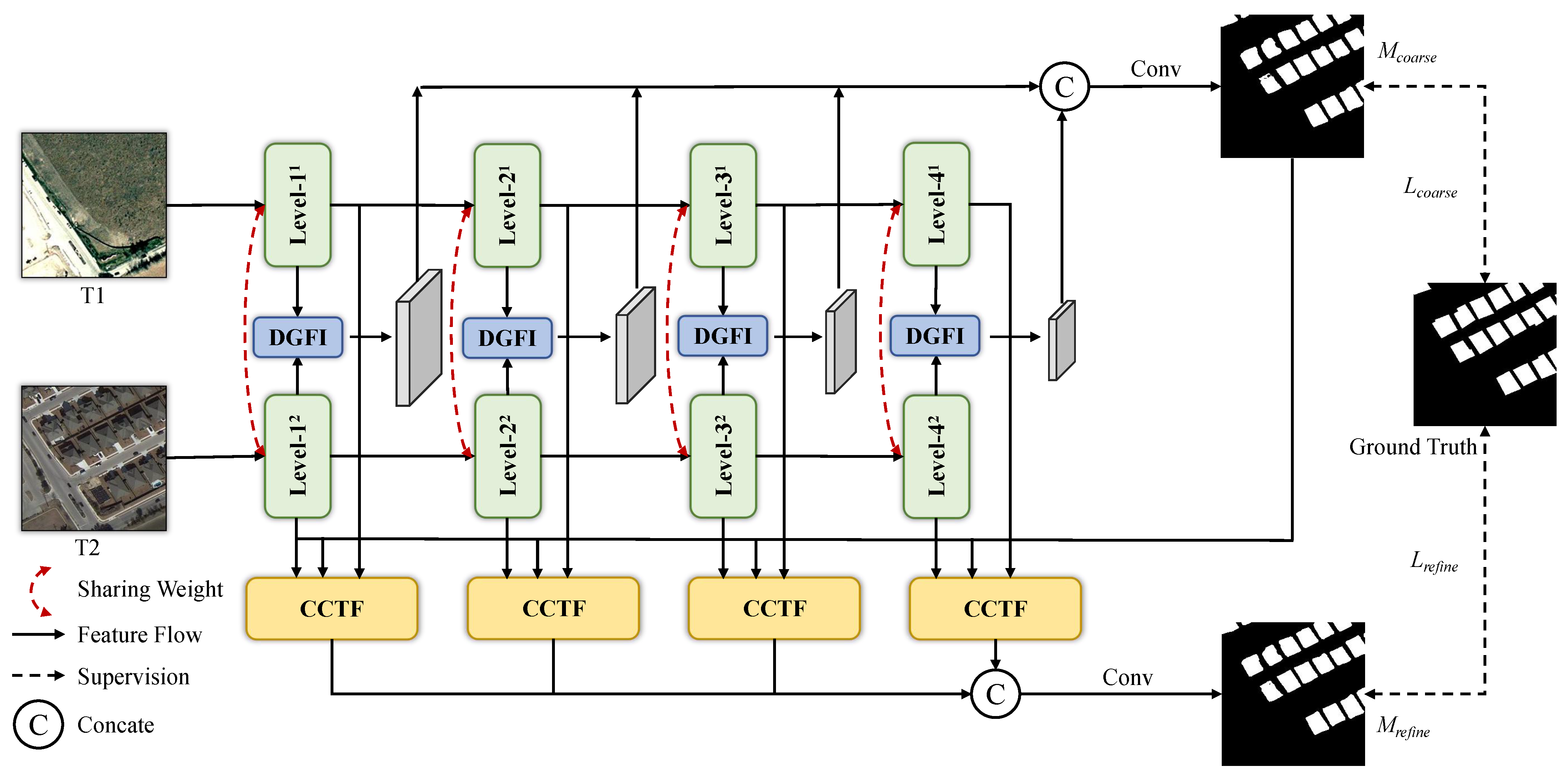
The overall architecture of DCAFNet is illustrated in Figure 2. The proposed network adopts a two-stage coarse-to-fine framework that progressively refines change predictions, and mainly consists of three parts: the feature extraction backbone network, the Difference-Gated Feature Interaction module, and the Change-Aware Cross-Temporal Fusion module.

We employ MobileNetV2 [41] as the feature extraction backbone based on the performance-efficiency analysis in Section 5.5. In our Siamese configuration, both temporal images $T1$ and $T2$ share identical encoder weights. This process yields four pairs of multi-level feature maps: $Level\text{-}{i}^1$ and $Level\text{-}{i}^2$ (for $i=1,2,3,4$), which we denote as ${\mathbf{F}}_A^i$ and ${\mathbf{F}}_B^i$, respectively. These extracted feature levels correspond to spatial resolutions of 64 × 64, 32 × 32, 16 × 16, and 8 × 8. The algorithm flow proceeds as follows: the bitemporal features are first processed through the DGFI module to produce ${\mathbf{F}}_{DGFI}^i$, which are then upsampled, concatenated, and decoded to generate the coarse change map $M_{coarse}$. Subsequently, the original backbone features ${\mathbf{F}}_A^i$ and ${\mathbf{F}}_B^i$, together with $M_{coarse}$, are refined through the CCTF module to yield ${\mathbf{F}}_{out}^i$, which are decoded to produce the final refined change map $M_{refine}$. Algorithm 1 summarizes this process, where GCCM and GRCM denote the coarse and refined change map generation stages, respectively.

Algorithm 1 Inference of DCAFNet.

Require: a pair of bitemporal remote sensing images: $\left\{\right(T1,T2\left)\right\}$ Ensure: $M_{refine}$ (a change map)   1: Extract multiscale feature group ${\mathbf{F}}_A^i$ from $T1$   2: Extract multiscale feature group ${\mathbf{F}}_B^i$ from $T2$   3: Perform bitemporal feature fusion through the DGFI module. ${\mathbf{F}}_{DGFI}^i=\mathrm{DGFI}({\mathbf{F}}_A^i,{\mathbf{F}}_B^i),i=1,2,3,4$   4: Process ${\mathbf{F}}_{DGFI}^i$ through the GCCM step to generate a coarse change map. $M_{coarse}=\mathrm{GCCM}({\mathbf{F}}_{DGFI}^1,{\mathbf{F}}_{DGFI}^2,{\mathbf{F}}_{DGFI}^3,{\mathbf{F}}_{DGFI}^4)$   5: Combine the feature map and the coarse change map, refining the feature map using the CGFR module. $({\widehat{\mathbf{F}}}_A^i,{\widehat{\mathbf{F}}}_B^i)=\mathrm{CGFR}({\mathbf{F}}_A^i,{\mathbf{F}}_B^i,M_{coarse}),i=1,2,3,4$   6: Perform adaptive feature fusion on the refined features using CTAF module. ${\mathbf{F}}_{out}^i=\mathrm{CTAF}({\widehat{\mathbf{F}}}_A^i,{\widehat{\mathbf{F}}}_B^i),i=1,2,3,4$   7: Process ${\mathbf{F}}_{out}^i$ through the GRCM step to generate the predicted refined change map. $M_{refine}=\mathrm{GRCM}({\mathbf{F}}_{out}^1,{\mathbf{F}}_{out}^2,{\mathbf{F}}_{out}^3,{\mathbf{F}}_{out}^4)$

This coarse-to-fine architecture enables DCAFNet to simultaneously facilitate pseudo-change suppression (through the DGFI module) and missed detection reduction (through the CCTF module) within a unified framework.

3.2. Difference-Gated Feature Interaction Module

Motivation. To mitigate pseudo-changes in change detection, researchers have developed various feature-interaction strategies, including element-wise subtraction (FC-Siam-diff [10]), channel-wise concatenation (FC-Siam-conc [10], SNUNet [11]), and attention-guided approaches (DGANet [21], BiFA [22], among others). However, these paradigms exhibit distinct limitations. Static operations fail to adaptively filter environmental noise, while dynamic attention mechanisms typically act as general-purpose enhancers without explicitly modeling the magnitude of temporal differences. Consequently, neither can robustly discriminate genuine changes from pseudo-change interference. To overcome these limitations, we propose a Difference-Gated Adaptive Fusion mechanism that generates spatially varying gating signals based on difference magnitude. For unchanged regions, it performs weighted averaging to smooth spectral fluctuations; for changed regions, it provides a bounded positive residual bias to preserve genuine change signals.

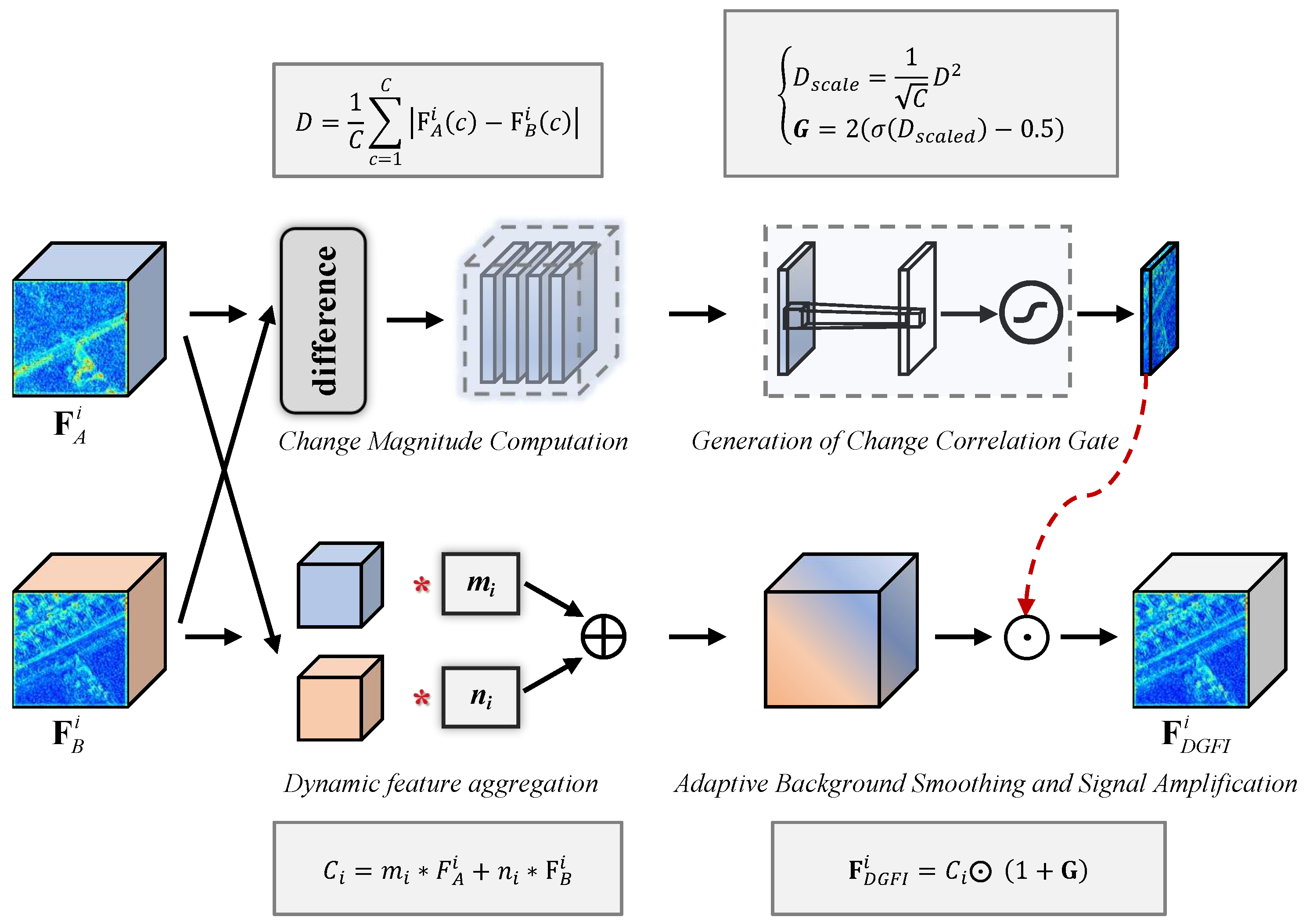
The DGFI module consists of three stages: (1) change magnitude computation via channel-wise mean absolute difference, (2) change correlation gate generation through nonlinear transformation, and (3) adaptive fusion with learnable weights modulated by the gating signal.

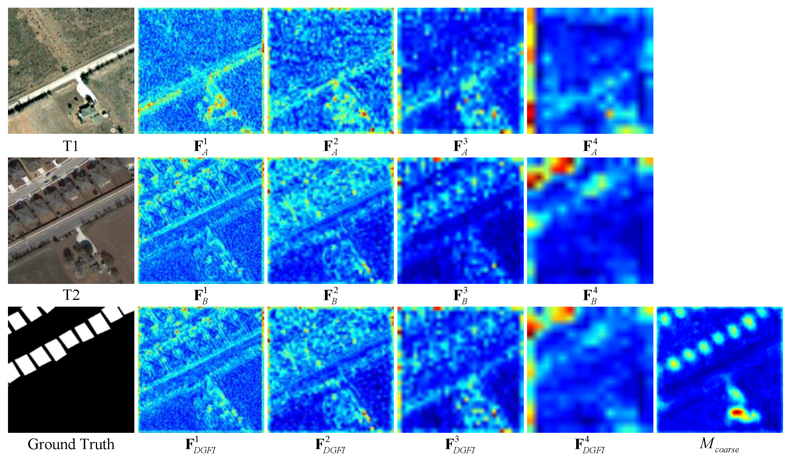
As illustrated in Figure 3, let ${\mathbf{F}}_A^i$ and ${\mathbf{F}}_B^i\in {\mathbb{R}}^{C\times H\times W}$ denote the feature maps extracted from the Siamese encoder at level i (where $i\in \{1,2,3,4\}$). Unlike conventional approaches that employ static subtraction or concatenation, we first compute the channel-wise mean absolute difference to capture the global intensity of spectral variations at each spatial position:

$$\mathcal{D}={\displaystyle \frac{1}{C}}{\displaystyle \sum _{c=1}^C}|{\mathbf{F}}_A^i\left(c\right)-{\mathbf{F}}_B^i\left(c\right)|$$

(1)

where C is the number of feature channels and $\mathcal{D}\in {\mathbb{R}}^{1\times H\times W}$ is a single-channel spatial map assigning a scalar difference magnitude to every position of the co-registered feature pair. It shares the spatial shape of ${\mathbf{F}}_A^i$ with one channel, and in the adaptive fusion of Equation (6), it is broadcast across the C channels through the element-wise product ⊙. Averaging over channels yields a change-magnitude estimate that is robust to channel-specific noise.

To enhance the signal-to-noise ratio and facilitate discrimination between genuine changes and pseudo-changes, we apply an element-wise squaring of $\mathcal{D}$ followed by a scalar normalization by the factor $1/\sqrt{C}$:

$${\mathcal{D}}_{scaled}=\left({\displaystyle \frac{1}{\sqrt{C}}}\right){\mathcal{D}}^2$$

(2)

The parentheses make explicit that $1/\sqrt{C}$ is a positive scalar applied uniformly at every position and is not part of the exponentiation, so ${\mathcal{D}}_{scaled}$ inherits the shape ${\mathbb{R}}^{1\times H\times W}$ of $\mathcal{D}$. This channel-dependent factor also keeps the pre-activation input bounded, preventing saturation of the subsequent sigmoid.

The choice of a quadratic transformation over a linear mapping is mathematically motivated by the residual behavior of the resulting gate in unchanged regions. Consider an unchanged pixel with a small residual difference $\mathcal{D}=\epsilon >0$, arising from sensor noise, minor misregistration, or subtle photometric variations. The first-order Taylor expansion of $\sigma$ around zero, $\sigma \left(x\right)\approx 0.5+x/4$ for small x, yields

$${\mathbf{G}}_{\mathrm{quad}}=2\sigma \left(\frac{{\epsilon }^2}{\sqrt{C}}\right)-1\approx \frac{{\epsilon }^2}{2\sqrt{C}}=\mathcal{O}\left({\epsilon }^2\right),$$

(3)

$${\mathbf{G}}_{\mathrm{lin}}=2\sigma \left(\frac{\epsilon }{\sqrt{C}}\right)-1\approx \frac{\epsilon }{2\sqrt{C}}=\mathcal{O}\left(\epsilon \right).$$

(4)

The quadratic gate therefore produces a residual response one order of magnitude smaller than the linear counterpart for small $\epsilon$. This behavior implements an implicit soft threshold: minor pseudo-changes are aggressively suppressed without requiring any explicit thresholding hyperparameter or external regularizer, while the response to progressively larger $\mathcal{D}$ remains smoothly differentiable. This squared-magnitude formulation is aligned with classical signal-processing precedents where the squared magnitudes of a residual are used as the primary detection statistic [42]. An empirical comparison between the quadratic and linear scaling is provided in Section 5.2, and the effectiveness of the implicit soft threshold is quantitatively verified in Section 5.9.

The enhanced difference map ${\mathcal{D}}_{scaled}$ is then mapped to a normalized gating signal $\mathbf{G}\in {\mathbb{R}}^{1\times H\times W}$ via a shifted Sigmoid function:

$$\mathbf{G}=2·\left(\sigma \left({\mathcal{D}}_{scaled}\right)-0.5\right)$$

(5)

where $\sigma (·)$ represents the Sigmoid function. Since ${\mathcal{D}}_{scaled}\ge 0$, the term $\sigma \left({\mathcal{D}}_{scaled}\right)$ lies in the range $[0.5,1.0]$. The transformation $2(·-0.5)$ rescales this to approximately $[0,1]$. Consequently, $\mathbf{G}\approx 0$ indicates high confidence in an unchanged state, while $\mathbf{G}\approx 1$ indicates a changed state.

Finally, we fuse the bitemporal features using learnable weights $m_i$ and $n_i$ to construct an optimized background representation. This representation is then modulated by the change correlation gate:

$${\mathbf{F}}_{DGFI}^i=(m_i·{\mathbf{F}}_A^i+n_i·{\mathbf{F}}_B^i)\odot (1+\mathbf{G})$$

(6)

where ⊙ denotes element-wise multiplication, and $m_i$, $n_i$ are learnable scalar parameters initialized to 1.0.

This formulation achieves a dual effect that distinguishes it from prior feature interaction methods:

• For Unchanged Regions ($\mathbf{G}\to 0$): The module outputs approximately $m_i{\mathbf{F}}_A^i+n_i{\mathbf{F}}_B^i$. By learning optimal $m_i$ and $n_i$, the network effectively performs weighted averaging of the bitemporal features. This cancels out random spectral fluctuations caused by pseudo-changes (e.g., illumination differences, seasonal variations), stabilizing the background representation and reducing false alarms.
• For Changed Regions: The modulation factor $(1+\mathbf{G})$ produces a bounded, monotonically increasing residual response with respect to the local difference magnitude $\mathcal{D}$. This provides a systematic positive bias in genuine change regions while, by construction, remaining conservative in absolute magnitude (the implicit soft-threshold behavior derived above). The effect is to preserve subtle change signals from being overwhelmed by background features during subsequent downsampling operations, without introducing excessive amplification that could destabilize training. Statistical verification of this behavior across three benchmarks is presented in Section 5.9.

Theoretical properties of the gate operator. The bounded and monotone behavior invoked above, together with the second-order noise attenuation derived earlier, can be established formally. Since every operation involved is element-wise, we regard $\mathbf{G}$ here as a scalar function of $\mathcal{D}$ at a single spatial position. First, because ${\mathcal{D}}_{scaled}\ge 0$, we have $\mathbf{G}\in [0,1)$ and therefore $(1+\mathbf{G})\in [1,2)$: the gate amplifies the fused background $m_i{\mathbf{F}}_A^i+n_i{\mathbf{F}}_B^i$ by at most a factor of two and never attenuates it, so no element of ${\mathbf{F}}_{DGFI}^i$ can exceed twice the corresponding fused background value (boundedness ⇒ forward stability). Second, $\mathbf{G}$ is the composition of the monotonically increasing map $\mathcal{D}\mapsto {\mathcal{D}}^2$ on $[0,\infty )$, the positive rescaling by $1/\sqrt{C}$, and $\sigma$; it is therefore non-decreasing in $\mathcal{D}$, i.e., an order-preserving mapping from difference magnitude to change confidence (monotonicity). Third, direct differentiation yields

$${\displaystyle \frac{d\mathbf{G}}{d\mathcal{D}}}={\displaystyle \frac{4\mathcal{D}}{\sqrt{C}}}\sigma \left({\mathcal{D}}_{scaled}\right)\left(1-\sigma \left({\mathcal{D}}_{scaled}\right)\right),$$

(7)

which is continuous, vanishes at $\mathcal{D}=0$, and decays exponentially as $\mathcal{D}\to \infty$; it is thus globally bounded, making $\mathbf{G}$ globally Lipschitz in $\mathcal{D}$. Bounded input perturbations (such as sensor noise or slight misregistration) therefore produce bounded gate perturbations (Lipschitz continuity ⇒ robustness). Together with the $\mathcal{O}\left({\epsilon }^2\right)$ attenuation established above, these properties provide a formal, operator-level justification of the stability and robustness of the DGFI design; empirical verification across three benchmarks is presented in Section 5.2 and Section 5.9.

Behaviour under varying sensor noise levels. Sensor noise contributes to the small residual $\mathcal{D}=\epsilon >0$ at an unchanged pixel, so the quadratic scaling gives $\mathbf{G}\approx {\epsilon }^2/\left(2\sqrt{C}\right)=\mathcal{O}\left({\epsilon }^2\right)$: the gate response grows quadratically, not linearly, with the noise standard deviation, and remains bounded to a negligible residual within the second-order Taylor regime (i.e., moderate noise levels). Empirically, the mean amplification ${\overline{1+G}}_u$ over unchanged pixels stays within $[1.0025,1.0096]$ across the three benchmarks (Section 5.9), confirming this graceful degradation.

After obtaining the four levels of DGFI-processed features ${\mathbf{F}}_{DGFI}^i$ ($i=1,2,3,4$), we first apply convolutional layers to refine features at each level:

$$\begin{array}{cc}\hfill {\mathbf{F}}_{DGFI}^{4^{\prime }}& ={\mathrm{Conv}}_4\left({\mathbf{F}}_{DGFI}^4\right)\hfill \\ \hfill {\mathbf{F}}_{DGFI}^{3^{\prime }}& ={\mathrm{Conv}}_3\left({\mathbf{F}}_{DGFI}^3\right)\hfill \\ \hfill {\mathbf{F}}_{DGFI}^{2^{\prime }}& ={\mathrm{Conv}}_2\left({\mathbf{F}}_{DGFI}^2\right)\hfill \end{array}$$

(8)

where ${\mathrm{Conv}}_i$ represents sequential BasicConv2d blocks (each comprising a $3\times 3$ convolution, batch normalization, and ReLU activation). We then upsample all feature maps to match the spatial resolution of ${\mathbf{F}}_{DGFI}^1$ using bilinear interpolation and concatenate them along the channel dimension:

$${\mathbf{F}}_{coarse}=\mathrm{Concat}({\mathbf{F}}_{DGFI}^1,{\mathbf{F}}_{DGFI}^{2^{\prime }},{\mathbf{F}}_{DGFI}^{3^{\prime }},{\mathbf{F}}_{DGFI}^{4^{\prime }})$$

(9)

The concatenated features are processed through the coarse decoder, which progressively reduces channel dimensionality through a series of BasicConv2d layers, culminating in a final convolutional layer that produces the two-channel coarse change map $M_{coarse}$.

Remarks. Unlike static operators (FC-Siam-diff, FC-Siam-conc [10], SNUNet [11]) that apply uniform feature interaction without explicit change modeling, DGFI generates a change correlation gate $\mathbf{G}$ providing spatially varying modulation based on change magnitude; Section 3.4 further contrasts this design with attention-based interaction. The ablation results in Section 5.2 validate its effectiveness.

3.3. Change-Aware Cross-Temporal Fusion Module

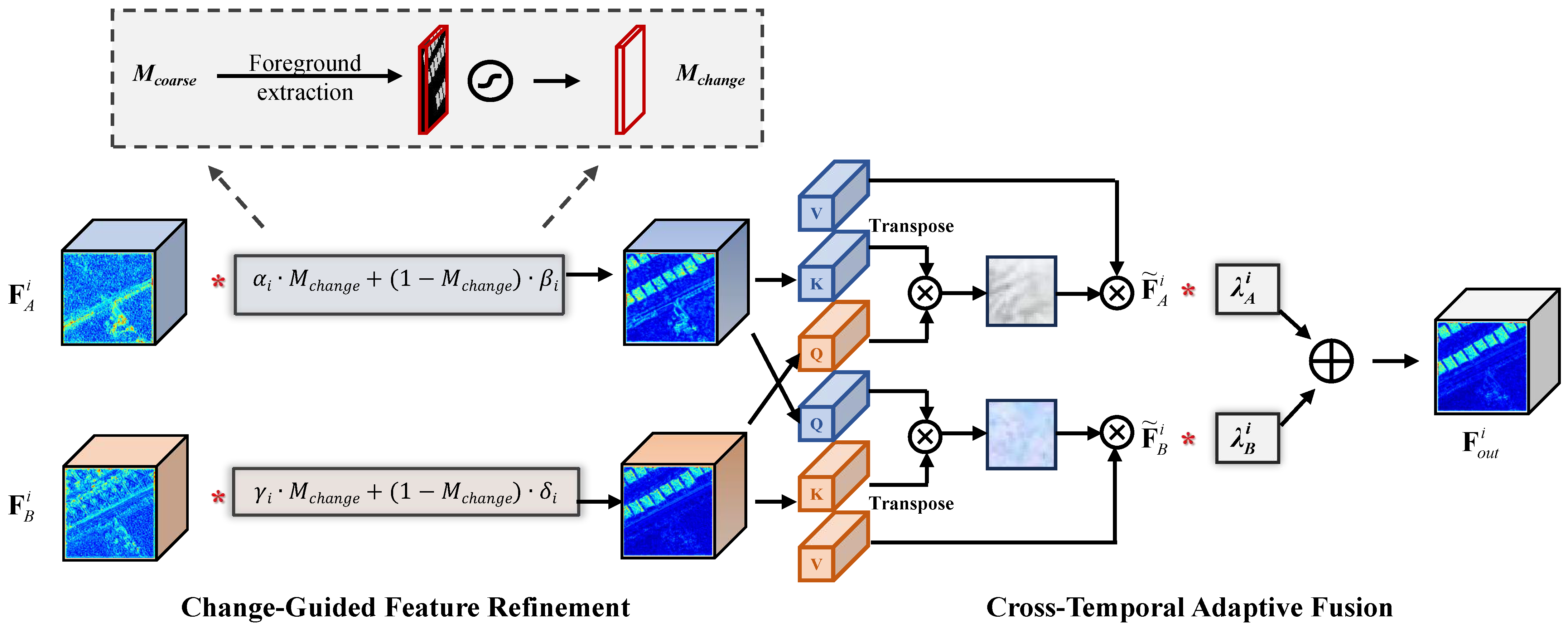
Motivation. Existing remedies for missed detections include cross-layer fusion (CLNet [26]), multiscale Transformer fusion (M-Swin [27]), mask classification (MaskCD [28]) and coarse-to-fine refinement [29]. In these frameworks, the coarse prediction is largely propagated rather than used as explicit semantic feedback that recalibrates backbone features before temporal interaction. CCTF therefore comprises CGFR, which modulates backbone features through learnable foreground–background weighting driven by the coarse prediction, and CTAF, which performs bidirectional cross-temporal attention with adaptive fusion to cope with unequal image quality. 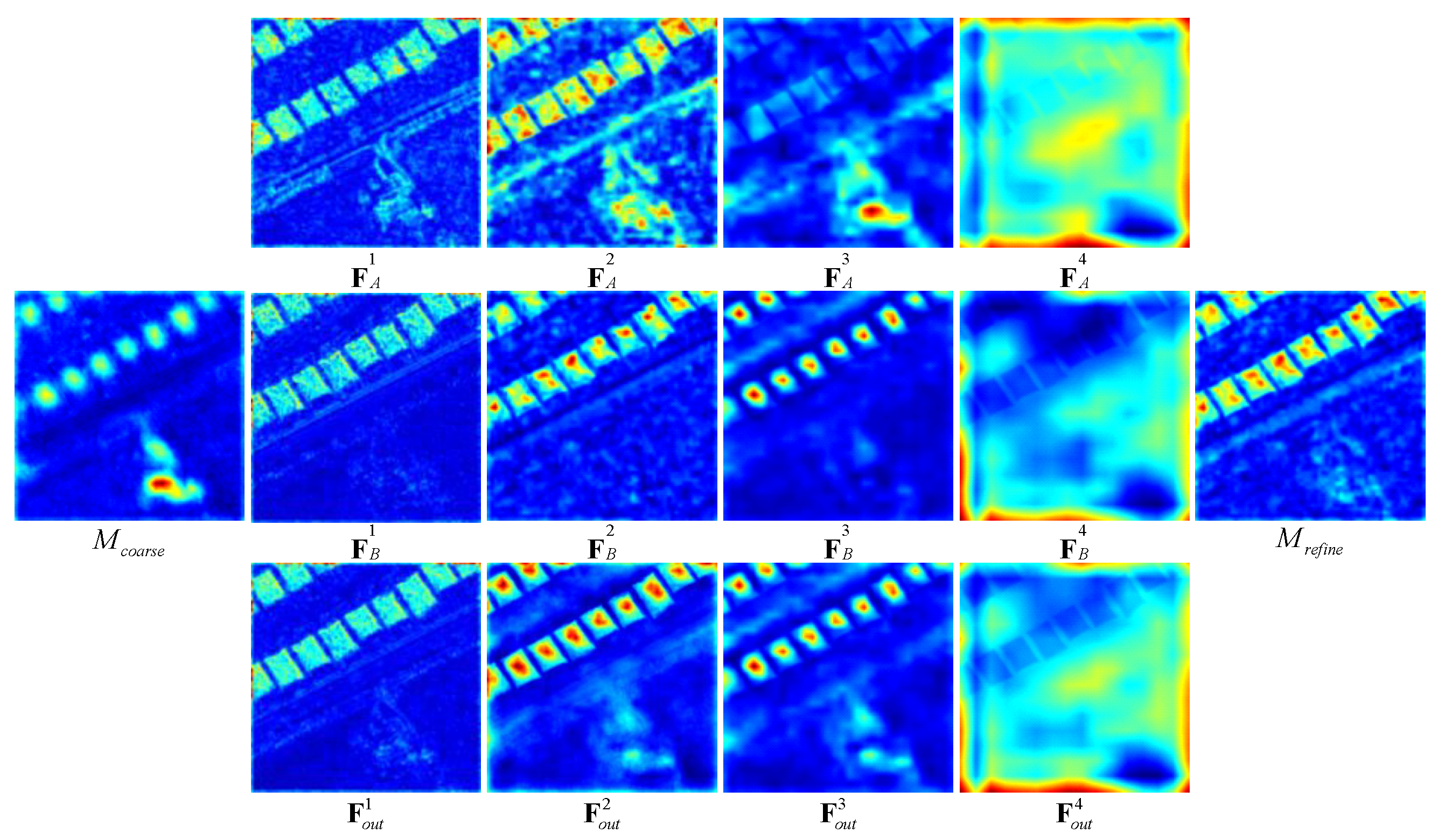Its architecture is shown in Figure 4.

(1) Change-Guided Feature Refinement Module

The CGFR module recalibrates the original backbone features based on the preliminary change predictions. This design is motivated by the observation that existing refinement strategies operate independently of initial detection results, missing the opportunity to use coarse predictions as semantic guidance for targeted enhancement.

First, the change probability map is extracted and normalized from the coarse prediction:

$$M_{change}=\sigma \left(M_{coarse}[1,:,:]\right)$$

(10)

where $M_{coarse}[1,:,:]$ represents the change channel of the two-class coarse prediction, and $\sigma (·)$ is the Sigmoid function that produces probability values in the range $(0,1)$.

We then explicitly model the contributions of both the foreground (potential changes) and the background (unchanged areas) using four learnable scalar parameters for each feature level: ${\alpha }_i$ and ${\beta }_i$ for temporal branch A, and ${\gamma }_i$ and ${\delta }_i$ for temporal branch B. Let ${\mathrm{Proj}}^i(·)$ denote the level-i $3\times 3$ convolutional projection and $\mathrm{Up}(·)$ the bilinear upsampling to the resolution of $M_{change}$, and write ${\mathbf{F}}_A^{i\prime }=\mathrm{Up}\left({\mathrm{Proj}}^i\left({\mathbf{F}}_A^i\right)\right)$ (and ${\mathbf{F}}_B^{i\prime }$ analogously).

The refined features ${\widehat{\mathbf{F}}}_A^i$ and ${\widehat{\mathbf{F}}}_B^i$ are computed as follows:

$$\begin{array}{cc}\hfill {\widehat{\mathbf{F}}}_A^i& ={\mathbf{F}}_A^{i\prime }\odot ({\alpha }_i·M_{change}+{\beta }_i·(\mathbf{1}-M_{change}))\hfill \\ \hfill {\widehat{\mathbf{F}}}_B^i& ={\mathbf{F}}_B^{i\prime }\odot ({\gamma }_i·M_{change}+{\delta }_i·(\mathbf{1}-M_{change}))\hfill \end{array}$$

(11)

where $\mathbf{1}$ denotes a tensor of ones with the same spatial dimensions as $M_{change}$. Both $M_{change}$ and $(\mathbf{1}-M_{change})$ have shape ${\mathbb{R}}^{1\times H\times W}$; each of the four scalar-weighted combinations therefore also has shape ${\mathbb{R}}^{1\times H\times W}$ and is broadcast across the C channels of the projected feature ${\mathbf{F}}_A^i$ or ${\mathbf{F}}_B^i$ during the element-wise product ⊙.

This mechanism is critical for recovering missed detections. Consider the scenario where the coarse map misses a subtle change (i.e., $M_{change}$ is low in a genuine change region). During training, the network can learn larger weights for ${\beta }_i$ or ${\delta }_i$ (the background-associated weights) to amplify features in regions initially predicted as unchanged, providing subsequent layers a second opportunity to detect the subtle signal that was initially overlooked. Conversely, in regions where $M_{change}$ is high, the foreground weights ${\alpha }_i$ and ${\gamma }_i$ can emphasize change-related features. This adaptive weighting scheme enables the network to differentially process features based on their predicted change status, facilitating the correction of localized false positives, confirmation of genuine changes, and recovery of subtle missed ones.

(2) Cross-Temporal Adaptive Fusion module

The CTAF module employs a multi-head cross-attention mechanism to model inter-temporal dependencies, followed by learnable adaptive fusion for robust feature synthesis. Unlike self-attention, which models intra-image context, we design a bidirectional cross-attention mechanism to capture cross-temporal relationships. The refined features ${\widehat{\mathbf{F}}}_A^i$ and ${\widehat{\mathbf{F}}}_B^i$ are first reshaped from ${\mathbb{R}}^{C\times H\times W}$ to ${\mathbb{R}}^{HW\times C}$ and then projected into Query ($\mathbf{Q}$), Key ($\mathbf{K}$), and Value ($\mathbf{V}$) spaces through learnable linear transformations.

The crucial design choice is that we use features from one temporal phase to query the other, rather than performing self-attention within each temporal branch. For temporal branch A, we compute the attention map using ${\mathbf{K}}_A$ and ${\mathbf{Q}}_B$, and aggregate global context from ${\mathbf{V}}_A$. This operation effectively highlights features in image A that are semantically relevant or distinct with respect to image B. To ensure numerical stability, we apply $L_2$ normalization to the query and key vectors before computing attention scores.

The cross-attention operation is formulated as

$$\mathrm{CrossAttn}({\mathbf{X}}_s,{\mathbf{X}}_g)=\mathrm{Softmax}\left({\displaystyle \frac{{\mathbf{K}}_s{\mathbf{Q}}_g^T}{\sqrt{d_k}}}\right){\mathbf{V}}_s$$

(12)

where the subscripts s and g denote source and guide, respectively, and $d_k$ denotes the dimension per attention head. Applying this operation bidirectionally yields two interaction-enhanced feature maps:

$${\tilde{\mathbf{F}}}_A^i=\mathrm{CrossAttn}({\widehat{\mathbf{F}}}_A^i,{\widehat{\mathbf{F}}}_B^i),{\tilde{\mathbf{F}}}_B^i=\mathrm{CrossAttn}({\widehat{\mathbf{F}}}_B^i,{\widehat{\mathbf{F}}}_A^i)$$

(13)

This bidirectional design enables comprehensive cross-temporal modeling: ${\tilde{\mathbf{F}}}_A^i$ encodes features from $T1$ that are relevant to changes observed from the perspective of $T2$, while ${\tilde{\mathbf{F}}}_B^i$ captures the complementary relationship. This mutual information exchange facilitates the identification of subtle changes that might be apparent only when considering both temporal contexts simultaneously.

To synthesize the processed bitemporal information into a unified feature representation for decoding, we propose a learnable adaptive fusion strategy. In contrast to static fusion schemes (e.g., concatenation or element-wise addition) that assume equal contributions from both temporal branches, we define level-specific learnable weights ${\lambda }_A^i$ and ${\lambda }_B^i$. The final output of the CCTF module is computed as:

$${\mathbf{F}}_{out}^i={\lambda }_A^i·{\tilde{\mathbf{F}}}_A^i+{\lambda }_B^i·{\tilde{\mathbf{F}}}_B^i$$

(14)

This adaptive weighting mechanism is particularly important for handling varying image quality conditions. When one temporal image is degraded by clouds, shadows, or sensor noise, the network can automatically assign lower weights to features from the degraded image, ensuring robust feature synthesis. The weights are initialized to 1.0 and learned jointly with other network parameters during end-to-end training.

The refined decoder follows an analogous structure. The CCTF-processed features ${\mathbf{F}}_{out}^i$ are concatenated and decoded:

$${\mathbf{F}}_{refine}=\mathrm{Concat}({\mathbf{F}}_{out}^1,{\mathbf{F}}_{out}^2,{\mathbf{F}}_{out}^3,{\mathbf{F}}_{out}^4)$$

(15)

The refined decoder processes ${\mathbf{F}}_{refine}$ to produce the final two-channel refined change map $M_{refine}$. Both $M_{coarse}$ and $M_{refine}$ are upsampled to the original input resolution using bilinear interpolation before loss computation.

Remarks. CCTF implements a predict-then-refine paradigm in which the coarse prediction actively recalibrates backbone features before cross-temporal interaction. Its distinction from conventional refinement and self-attention designs is analyzed in Section 3.4, and the ablation results in Section 5.4 validate the synergistic effect of its components.

3.4. Distinction from Existing Mechanisms

DCAFNet builds on established paradigms (feature differencing, attention, coarse-to-fine refinement, and cross-temporal interaction) which we adopt without claiming them as novel. What we claim are four mechanism-level design choices, each isolated by a dedicated ablation.

DGFI vs. adaptive weighting on difference features. Adaptive weighting (e.g., AbsDiff+CBAM [43], DGANet [21], BiFA [22]) re-scales the difference tensor as a feature without modeling the mapping from difference magnitude to change probability. DGFI derives its gate solely from $\mathcal{D}$ through ${\mathcal{D}}^2/\sqrt{C}$, whose expansion in Section 3.2 gives an $O\left({\epsilon }^2\right)$ residual response, one order below the $O\left(\epsilon \right)$ of a linear-magnitude gate, suppressing pseudo-changes without any thresholding hyperparameter, following the squared-magnitude detection principle of CFAR [42]. Accordingly, DGFI exceeds AbsDiff+CBAM by $+0.13/+0.23/+0.15$ F1 (Section 5.2), and the gate alone attains a pixel-wise ROC-AUC of $0.933/0.952/0.800$ (Section 5.9.1).

CGFR vs. coarse-mask-guided refinement. Direct masking $\widehat{\mathbf{F}}=\mathbf{F}\odot M_{change}$ suppresses features wherever the coarse map reads “unchanged”, discarding precisely the evidence required to recover missed detections, whereas the re-weighting of Equation (11) retains and re-amplifies them through learned $\beta ,\delta >0$. Direct masking underperforms CGFR by $0.62/0.63/0.27$ F1 and inverse masking falls below the “w/o CGFR” baseline (Section 5.3), while the learned background weights remain consistently non-negligible (Section 5.9.3).

CTAF vs. standard cross-temporal interaction. Because change is defined only through cross-temporal correspondence, CTAF replaces the intra-temporal self-attention of BIT [13] and ChangeFormer [14] with bidirectional cross-attention, fused by level-specific learnable weights instead of fixed concatenation. The ablation in Section 5.4 isolates both choices: +0.13/+0.22/+0.14 F1 and +0.11/+0.11/+0.13 F1, respectively.

Coarse map as an active prior rather than a supervision target. Existing coarse-to-fine methods use $M_{coarse}$ mainly as a deep-supervision target, whereas DCAFNet feeds it back through CGFR to recalibrate backbone features. The leave-one-out ablation shows that removing any single module costs $0.58$–$0.85$% average F1, indicating that the gains arise from complementary mechanisms rather than from stacked parameters.

3.5. Loss Function

We employ the standard Cross-Entropy (CE) loss for pixel-wise classification. For a predicted map $\mathbf{P}\in {\mathbb{R}}^{H\times W\times 2}$ and the ground truth label $\mathbf{Y}\in {\{0,1\}}^{H\times W}$, the loss is formulated as

$$L_{ce}(\mathbf{P},\mathbf{Y})=-{\displaystyle \frac{1}{H\times W}}{\displaystyle \sum _{h=1}^H}{\displaystyle \sum _{w=1}^W}{\displaystyle \sum _{c=0}^1}{\mathbf{Y}}_{(h,w,c)}log\left({\mathbf{P}}_{(h,w,c)}\right)$$

(16)

where H and W denote the spatial dimensions, and c represents the class index for changed ($c=1$) or unchanged ($c=0$) pixels. To facilitate progressive refinement, we adopt a weighted deep supervision strategy. For notational brevity, we denote $L_{refine}=L_{ce}(M_{refine},\mathbf{Y})$ and $L_{coarse}=L_{ce}(M_{coarse},\mathbf{Y})$. The total objective function is defined as

$$L_{total}=L_{refine}+\lambda L_{coarse}$$

(17)

where $\lambda$ balances the contribution of the coarse supervision, which provides meaningful gradients to the DGFI module, against the refined supervision that guides precise boundary delineation. Based on sensitivity analysis (Section 5.6), we set $\lambda =0.4$.

4. Experiments

4.1. Datasets

(1) LEVIR-CD [44]: The LEVIR-CD dataset records a time span of up to 16 years to observe and analyze long-term changes in buildings. The dataset also includes information on various environmental conditions, such as sensor characteristics, atmospheric conditions, seasonal conditions, and lighting conditions, providing the possibility to study the relationship between building changes and environmental factors. The official dataset settings specify that there are 7120 images in the training set, 1024 images in the validation set, and 2048 images in the test set.

(2) WHU-CD [45]: This dataset contains images of the reconstruction areas after the 6.3 magnitude earthquake in February 2011. The aerial images obtained in April 2012 cover 20.5 square kilometers and include 12,796 buildings. The aerial images obtained in 2016 for the same area include 16,077 buildings. These remote sensing images have dimensions of 32,507 × 15,354 pixels. The images are categorized into 7434 pairs using the principle of non-overlapping. Subsequently, these images are randomly distributed into training, validation, and test sets at a ratio of 8:1:1.

(3) CDD [46]: We employed the CDD dataset, which consists of 7 sets of images capturing seasonal changes. Each image pair has a size of $4725\times 2700$ pixels. Additionally, there are 4 pairs of images with a resolution of $1900\times 1000$ pixels. This dataset encompasses a wide range of objects varying in size, ranging from cars to massive architectural structures. It also captures the seasonal fluctuations, spanning from solitary trees to extensive forest tracts. The dataset is created by randomly rotating and cropping images to a size of $256\times 256$ pixels. In total, there are 16,000 images, with 10,000 utilized for training, 3000 for validation, and 3000 for testing.

(4) SYSU-CD [47]: The SYSU-CD dataset contains 20,000 aerial image pairs of size $256\times 256$, collected over Hong Kong from 2007 to 2014. Different from building-oriented datasets such as LEVIR-CD and WHU-CD, SYSU-CD includes diverse change categories, such as newly built urban buildings, suburban dilation, groundwork before construction, vegetation change, road expansion, and coastal construction. These heterogeneous changes make SYSU-CD a more challenging benchmark for evaluating the generalization ability of change detection methods. Following the official split, we use 12,000 pairs for training, 4000 for validation, and 4000 for testing.

4.2. Evaluation Metrics

We present six essential metrics, namely, precision (Pre.), recall (Rec.), F1-score (F1), intersection over union (IOU), overall accuracy (OA), and Kappa for evaluating the performance of predicted change maps compared to the ground truth (GT). The specific definitions of the metrics are as follows:

$$\begin{array}{cc}\hfill & \mathrm{Precision}={\displaystyle \frac{TP}{TP+FP}}\hfill \end{array}$$

(18)

$$\begin{array}{cc}\hfill & \mathrm{Recall}={\displaystyle \frac{TP}{TP+FN}}\hfill \end{array}$$

(19)

$$\begin{array}{cc}\hfill & \mathrm{F}1={\displaystyle \frac{2}{{\mathrm{Recall}}^{-1}+{\mathrm{Precision}}^{-1}}}\hfill \end{array}$$

(20)

$$\begin{array}{cc}\hfill & \mathrm{IOU}={\displaystyle \frac{TP}{TP+FP+FN}}\hfill \end{array}$$

(21)

$$\begin{array}{cc}\hfill & \mathrm{OA}={\displaystyle \frac{TP+TN}{TP+TN+FP+FN}}\hfill \end{array}$$

(22)

$$\begin{array}{cc}\hfill & \mathrm{Kappa}={\displaystyle \frac{OA-P}{1-P}}\hfill \end{array}$$

(23)

The variables TP, TN, FP, and FN correspond to the values of true positive, true negative, false positive, and false negative, respectively. The hypothetical probability of chance agreement, denoted P, is a key component of the Kappa calculation and is defined as

$$P={\displaystyle \frac{(\mathrm{TP}+\mathrm{FP})(\mathrm{TP}+\mathrm{FN})+(\mathrm{FN}+\mathrm{TN})(\mathrm{FP}+\mathrm{TN})}{{(\mathrm{TP}+\mathrm{FP}+\mathrm{TN}+\mathrm{FN})}^2}}$$

(24)

The F1-score is a comprehensive evaluation statistic that provides insights into the performance of the suggested algorithm by combining precision and recall metrics. Additionally, precision, recall, F1, IOU, OA, and Kappa serve as indicators of general model behavior, with higher values reflecting improved detection accuracy.

4.3. Implementation Details

The network we developed is trained and evaluated on an NVIDIA Titan RTX (24 GB) GPU hardware using the PyTorch 1.10.2 framework with CUDA 11.3. During training, the batch size is set to 16 and the initial learning rate is ${10}^{-4}$. The network is optimized with AdamW wrapped with Lookahead, and the initial learning rate of ${10}^{-4}$ is adjusted by a CosineAnnealingWarmRestarts schedule. The training dataset is trained for 225 epochs to ensure convergence of the network model. The network model that achieves the highest performance during the 225 epochs is chosen to evaluate its performance on the test set.

The MobileNetV2 backbone is initialized from ImageNet-pretrained weights. The newly introduced convolutional and linear layers retain the default PyTorch initialization; batch-normalization layers are initialized with (weight, bias) $=(1,0)$. The learnable scalars $m_i,n_i$ in the DGFI module (Section 3.2), ${\alpha }_i,{\beta }_i,{\gamma }_i,{\delta }_i$ in the CGFR module, and ${\lambda }_A^i,{\lambda }_B^i$ in the CTAF module are each initialized to one, so that all fusion and refinement modules start from an identity-like state and learn their relative emphasis during training.

Table 1. Per-level feature dimensions of DCAFNet for a $256\times 256$ input.

Level-i	Spatial Scale	Resolution	Channels C
1	$1/4$	$64\times 64$	24
2	$1/8$	$32\times 32$	32
3	$1/16$	$16\times 16$	96
4	$1/32$	$8\times 8$	320

lists the tensor shape at each level of the Siamese MobileNetV2 encoder for a $256\times 256$ input. The DGFI, CGFR, and CTAF modules operate level-wise and preserve the channel count C; the coarse and refined decoders bilinearly upsample all four levels to the $1/4$ scale before concatenation.

4.4. Comparisons with State-of-the-Art Methods

In order to assess the efficacy of our proposed DCAFNet, we conducted a comparative analysis with several state-of-the-art models. For a fair comparison, all comparison methods were retrained under identical experimental conditions using our hardware and software environment. These typical models include the following: FC-Siam-conc [10], FC-Siam-diff [10], BIT [13], SNUNet [11], ChangeFormer [14], ScratchFormer [37], GCD-DDPM [18], ChangeMamba [15], SFEARNet [32], DCSI-UNet [16].

(1) FC-Siam-conc [10] and (2) FC-Siam-diff [10] fuse multiscale Siamese features by concatenation and by differencing, respectively. (3) BIT [13] encodes bitemporal features as compact semantic tokens and models their spatiotemporal context with a Transformer encoder–decoder. (4) SNUNet [11] uses dense encoder–decoder skip connections. (5) ChangeFormer [14] pairs a multi-layer Transformer encoder with an MLP decoder. (6) ScratchFormer [37] applies shuffled sparse attention plus a channel-wise enhancement fusion module to suppress noisy changes. (7) GCD-DDPM [18] generates change maps with a denoising diffusion probabilistic model driven by multi-level change cues. (8) ChangeMamba [15] uses a spatiotemporal state-space backbone with near-linear sequence complexity and three complementary spatiotemporal relationship modeling mechanisms. (9) SFEARNet [32] combines a semantic flow mechanism against upsampling loss with edge-aware boundary refinement. (10) DCSI-UNet [16] is a dual-stream UNet with parallel channel group interaction, spatial Gaussian attention, and multilayer aggregation.

4.5. Quantitative Results Analysis

The quantitative comparison results for the LEVIR-CD, WHU-CD, and CDD test sets are presented in

Table 2. Quantitative comparison on the LEVIR-CD dataset. The best results are highlighted in bold. All values are in percentage (%).

Model	Pre.	Rec.	F1	IOU	OA	Kappa
FC-Siam-conc	86.81	67.66	76.05	61.36	97.83	74.81
FC-Siam-diff	86.55	74.38	80.00	66.68	98.11	79.33
BIT	91.95	88.57	90.23	82.19	99.02	89.71
SNUNet	91.66	88.48	90.04	81.89	99.00	89.51
ChangeFormer	91.53	88.86	90.17	82.10	99.01	89.63
ScratchFormer	91.46	86.55	88.94	80.08	98.90	88.36
GCD-DDPM	90.68	91.24	90.96	83.56	99.14	90.51
ChangeMamba	91.17	90.65	90.91	83.33	99.08	90.42
SFEARNet	92.21	88.85	90.49	82.64	99.05	89.99
DCSI-UNet	92.17	89.90	91.02	83.52	99.10	90.55
DCAFNet	92.77	90.79	91.75	84.76	99.17	91.33

,

Table 3. Quantitative comparison on the WHU-CD dataset. The best results are highlighted in Bold. All values are in percentage (%).

Model	Pre.	Rec.	F1	IOU	OA	Kappa
FC-Siam-conc	40.09	73.84	51.97	35.11	93.63	49.15
FC-Siam-diff	38.82	71.80	50.40	33.69	93.40	47.62
BIT	86.07	85.61	85.84	75.19	98.68	85.15
SNUNet	88.35	87.80	88.07	78.69	98.89	87.54
ChangeFormer	93.44	85.70	89.40	80.84	99.12	89.01
ScratchFormer	93.70	82.56	87.78	78.22	98.93	87.22
GCD-DDPM	92.79	92.29	92.54	86.52	99.39	92.22
ChangeMamba	93.06	92.25	92.65	86.31	99.32	92.29
SFEARNet	93.38	90.84	92.09	85.34	99.27	91.70
DCSI-UNet	94.21	91.49	92.83	86.62	99.35	92.53
DCAFNet	96.30	92.50	94.37	89.33	99.49	94.11

, and

Table 4. Quantitative comparison on the CDD dataset. The best results are highlighted in bold. All values are in percentage (%).

Model	Pre.	Rec.	F1	IOU	OA	Kappa
FC-Siam-conc	88.00	53.58	66.61	49.93	93.66	63.33
FC-Siam-diff	88.49	51.53	65.14	48.30	93.49	61.82
BIT	95.86	94.59	95.22	90.88	98.88	94.59
SNUNet	96.82	96.72	96.77	93.74	99.24	96.34
ChangeFormer	95.28	93.83	94.55	89.66	98.72	93.82
ScratchFormer	96.62	95.64	96.12	92.54	99.09	95.61
GCD-DDPM	94.76	95.10	94.93	90.56	98.87	94.29
ChangeMamba	96.56	96.92	96.74	93.69	99.23	96.30
SFEARNet	95.66	96.24	95.95	92.21	99.04	95.41
DCSI-UNet	96.26	97.45	96.85	93.89	99.25	96.42
DCAFNet	98.00	98.50	98.25	96.57	99.58	98.01

, respectively. DCAFNet obtains an F1-score of 91.75% and an IOU of 84.76% on the LEVIR-CD dataset, surpassing DCSI-UNet, the strongest competitor in F1, by 0.73% in F1 and 1.24% in IOU, respectively. DCAFNet outperforms DCSI-UNet on the WHU-CD dataset with F1 and IOU scores that are 1.54% and 2.71% higher, respectively. On the CDD dataset, DCAFNet achieves an F1-score of 98.25%, outperforming DCSI-UNet by 1.40%, making it the top performer on all three building-centric benchmarks. Notably, the margins of DCAFNet are consistently larger under the stricter IOU and Kappa metrics: relative to DCSI-UNet, DCAFNet improves IOU by 1.24%, 2.71%, and 2.68%, and Kappa by 0.78%, 1.58%, and 1.59% on LEVIR-CD, WHU-CD, and CDD, respectively. Since IOU penalizes false positives and false negatives more strictly than F1, and Kappa compensates for chance agreement, these larger margins indicate that the gains are concentrated on the pseudo-change and missed-detection pixels targeted by the proposed modules, rather than being a uniform gain across all pixels. Retrained under the same protocol, ChangeMamba attains F1-scores of 90.91%, 92.65%, and 96.74% on LEVIR-CD, WHU-CD, and CDD, placing it among the strongest baselines: it ranks third on WHU-CD and fourth on LEVIR-CD and CDD, in all cases, below DCAFNet. Its gap to DCAFNet is 0.84%, 1.72%, and 1.51% in F1 but 1.43%, 3.02%, and 2.88% in IOU, again locating the difference on false positives and false negatives. State-space scanning propagates global context along fixed traversal orders and thus strengthens each temporal branch, yet the fusion of the two branches is not conditioned on the local difference magnitude and no preliminary prediction is fed back to the encoder.

Unlike the three benchmarks above, which are dominated by building changes, SYSU-CD [47] covers heterogeneous change categories, including buildings, roads, vegetation, and coastal/water scenes, making it a stricter cross-domain generalization test. As shown in

Table 5. Quantitative comparison on the SYSU-CD dataset. The best results are highlighted in bold. All values are in percentage (%).

Model	Pre.	Rec.	F1	IOU	OA	Kappa
FC-Siam-conc	76.41	76.17	76.29	61.67	88.83	68.98
FC-Siam-diff	88.05	55.29	67.92	51.43	87.68	60.79
BIT	82.36	74.30	78.12	64.10	90.18	71.81
SNUNet	79.04	76.71	77.86	63.75	89.71	71.16
ChangeFormer	84.99	70.93	77.33	63.04	90.19	71.13
ScratchFormer	83.40	76.15	79.61	66.13	90.80	73.69
GCD-DDPM	82.08	79.87	80.96	68.01	91.14	75.19
ChangeMamba	81.98	80.37	81.17	68.31	91.20	75.43
SFEARNet	85.41	78.34	81.72	69.09	91.73	76.39
DCSI-UNet	82.90	80.22	81.54	68.83	91.43	75.96
DCAFNet	86.45	79.41	82.78	70.62	92.21	77.76

, DCAFNet achieves the best F1 ($82.78\%$), IOU ($70.62\%$), OA ($92.21\%$), and Kappa ($77.76\%$), outperforming the second-best SFEARNet by $1.06\%$ in F1 and $1.53\%$ in IOU. This indicates that DCAFNet maintains a favorable balance between false-alarm suppression and missed-detection recovery in heterogeneous land-cover scenarios.

Figure 5 visualizes the F1-scores of all compared methods across the three datasets. As shown in the figure, DCAFNet consistently achieves the highest F1-scores. This advantage can be attributed to two complementary mechanisms. First, the DGFI module employs Difference-Gated Adaptive Fusion to suppress pseudo-changes at the feature interaction stage, which is particularly effective on datasets with complex illumination variations. Second, the CCTF module establishes a coarse-to-fine semantic feedback loop, significantly improving the recovery of subtle missed detections in challenging scenes such as WHU-CD and CDD. While the recent DCSI-UNet employs parallel attention, it lacks explicit pseudo-change filtering and semantic feedback, which limits its performance under these conditions.

4.6. Qualitative Results Analysis

We selected representative change detection scenes from three datasets to compare the visual performance of different methods. The visualization results are presented in Figure 6, where red pixels indicate false positives (FP), green pixels indicate false negatives (FN), black pixels indicate true negatives (TN), and white pixels indicate true positives (TP). The qualitative analysis is organized around the two core challenges targeted in this work.

Pseudo-changes from illumination, shadow, and seasonal differences are the first challenge. In Figure 6b,f, shadows cast near buildings lead ScratchFormer and GCD-DDPM to produce large false-positive regions (red), while DCAFNet suppresses them. The seasonal case in Figure 6k is harder still: snow cover alters surface appearance and most competitors respond with extensive false positives, whereas DCAFNet remains stable by smoothing background variation while preserving genuine change signals.

Missed detections form the second challenge. For the small targets in Figure 6a,e,i, DCAFNet is closest to the ground truth with the fewest false negatives (green), which we attribute to the CCTF module recalibrating features under coarse-map guidance and enhancing subtle signals through cross-temporal attention. For the densely distributed building changes in Figure 6d,h, SNUNet and BIT leave noticeable gaps, while the learnable foreground–background weighting of CGFR recovers initially overlooked regions and yields more complete boundaries. The same pattern holds for the large irregular areas in Figure 6c,g,l and for the narrow roads and small vehicles in Figure 6j, where DCAFNet attains the smallest combined error area.

To further verify the generalization of DCAFNet on non-building and heterogeneous changes, we visualize four representative SYSU-CD scenes in Figure 7. Figure 7a shows a vegetation change case, where competing methods produce large false-positive regions caused by seasonal reflectance variations, while DCAFNet yields a cleaner prediction, demonstrating the pseudo-change suppression ability of DGFI. Figure 7b presents groundwork before construction, in which most baselines miss large parts of the subtle bare-soil change region, whereas DCAFNet recovers the contour more completely due to the missed-detection recovery capability of CGFR. In Figure 7c, DCAFNet provides more complete coverage and smoother boundaries for newly built urban buildings. Figure 7d shows another subtle groundwork case, where DCAFNet produces the smallest overall error area. These visual results indicate that the proposed DGFI and CGFR mechanisms remain effective on heterogeneous SYSU-CD scenarios beyond building-centric benchmarks.

Overall, the qualitative results demonstrate that DCAFNet substantially mitigates both pseudo-change interference and missed detections within a unified framework, achieving superior visual quality across diverse change-detection scenarios.

5. Discussion

5.1. Ablation Studies

To evaluate the effectiveness of each proposed component, we conducted systematic ablation experiments on three benchmark datasets: LEVIR-CD, WHU-CD, and CDD. The baseline represents the DCAFNet network without the DGFI, CGFR, and CTAF modules.

Table 6. Ablation study of the proposed modules in DCAFNet. Each row represents the progressive addition of modules to the baseline. A checkmark indicates that the corresponding component is included. The best results are highlighted in bold. All values are in percentage (%).

Baseline	DGFI	CGFR	CTAF	LEVIR-CD		WHU-CD		CDD
				F1	IOU	F1	IOU	F1	IOU
✓				89.17	80.48	91.89	85.01	96.62	93.38
✓	✓			90.29	82.28	92.74	86.35	97.26	94.75
✓	✓	✓		91.24	83.91	93.71	88.21	97.67	95.45
✓	✓	✓	✓	91.75	84.76	94.37	89.33	98.25	96.57

presents the performance when progressively adding each module. The incorporation of the DGFI module yields F1 improvements of 1.12%, 0.85%, and 0.64% on the LEVIR CD, WHU-CD, and CDD datasets, respectively. This improvement demonstrates that the difference-gated adaptive fusion mechanism effectively improves discriminability between genuine changes and pseudo-change noise. Notably, the improvement is most pronounced on LEVIR-CD, which contains diverse illumination conditions, validating the module’s capability in handling spectral variations.

Adding CGFR on top of DGFI further improves F1 by 0.95%, 0.97%, and 0.41%, confirming that coarse predictions used as semantic priors let the network recover potentially missed detections; the smaller gain on CDD reflects its higher baseline, where fewer missed detections remain. Adding CTAF yields a further 0.51%, 0.66%, and 0.58%, showing that cross-temporal attention combined with learnable adaptive fusion captures complementary information from the two temporal branches and outperforms static fusion.

As visualized in Figure 8, the F1 performance progressively increases as each module is added to the baseline, with all models converging stably during training. The complete DCAFNet achieves the highest and most stable performance across all datasets, demonstrating the synergistic contribution of the three proposed modules. This stability is not incidental. The $1/\sqrt{C}$ scaling in the gate generation of Section 3.2 bounds the pre-sigmoid input to $\mathcal{O}\left(1\right)$ regardless of the channel count C, preventing gate saturation across the four heterogeneous feature levels (see Table 1); combined with the $\mathcal{O}\left({\epsilon }^2\right)$ implicit soft threshold of the quadratic transform near $\mathcal{D}\approx 0$, this yields optimization behavior that is stable by construction. The smooth response to the loss coefficient $\lambda$ shown in Figure 9, with a stable optimum at $\lambda =0.4$ across all datasets, further confirms robustness to the reported training setting.

Table 7. Leave-one-out (LOO) ablation of DCAFNet’s three modules on LEVIR-CD, WHU-CD, and CDD. Each row removes a single module while keeping the other two intact. All values are reused from existing ablation rows under identical training settings, as indicated in the Source column and justified in the main text. Average ΔF1 is computed across the three benchmarks. The best results are highlighted in bold.

Variant	LEVIR-CD F1	WHU-CD F1	CDD F1	Avg. ΔF1	Source
Full DCAFNet	91.75	94.37	98.25	—	Main result
w/o DGFI	91.21	93.19	97.43	$-0.85$	Addition row (Table 8)
w/o CGFR	90.80	93.40	97.84	$-0.78$	w/o CGFR row (Table 9)
w/o CTAF	91.24	93.71	97.67	$-0.58$	+DGFI+CGFR row (Table 6)

provides a leave-one-out counterpart to the progressive stacking ablation in Table 6, isolating the individual contribution of each module in the presence of the other two. All three modules contribute a non-trivial gain: removing any single one degrades F1 by 0.58–0.85% on average across the three benchmarks. The “w/o DGFI” entry is realized via the Addition row in

Table 8. Comparison of different feature-interaction strategies in the DGFI module. The best results are highlighted in bold. All values are in percentage (%).

Model	LEVIR-CD		WHU-CD		CDD
	F1	IOU	F1	IOU	F1	IOU
Subtraction	91.08	83.62	93.04	86.98	97.18	94.51
w/o DGFI (Addition)	91.21	83.84	93.19	87.25	97.43	94.99
Multiplication	91.37	84.11	93.48	87.80	97.54	95.20
DGFI w/o gate	91.41	84.18	93.62	88.01	97.76	95.62
Concat+Conv	91.46	84.26	93.65	88.07	97.81	95.71
AbsDiff+Conv	91.52	84.37	93.87	88.45	97.89	95.87
AbsDiff+CBAM	91.62	84.54	94.14	88.94	98.10	96.27
Linear gate	91.68	84.64	94.23	89.09	98.17	96.41
DGFI	91.75	84.76	94.37	89.33	98.25	96.57

, which is mathematically equivalent to removing the DGFI module under our architecture: DGFI’s output feeds only the coarse decoder, while both CGFR and CTAF operate on the original backbone features (Algorithm 1); therefore, removing DGFI reduces to replacing $\mathrm{DGFI}(A,B)$ with the simplest non-parametric fusion $A+B$. Reusing existing ablation rows for the other two entries similarly ensures identical training settings and therefore fair comparison. The consistent degradation across the three LOO variants (0.58–0.85%) confirms that none of the three modules is redundant, and that DCAFNet’s performance emerges from genuine complementary mechanisms rather than from stacking alone.

5.2. Effectiveness of the DGFI Module

To validate the proposed DGFI module, we compared it against eight feature interaction strategies spanning static operations (subtraction, addition, multiplication), learned fusion (Concat+Conv and AbsDiff+Conv, both using $3\times 3$ convolutional layers), attention-based interaction (AbsDiff+CBAM [43]), and two mechanism-level variants of DGFI itself (DGFI w/o gate, Linear gate). All variants use the complete DCAFNet pipeline with only the first-stage interaction module replaced. Results are presented in Table 8. Among static operators, multiplication achieves the best F1 (91.37%, 93.48%, 97.54% on the three datasets) due to its inherent background suppression, while subtraction performs worst as it exposes all spectral variations without selective filtering. However, all static operations share a fundamental limitation: they cannot adaptively distinguish genuine changes from pseudo-change noise. The learned strategies Concat+Conv and AbsDiff+Conv progressively improve performance by introducing trainable parameters and explicit difference modeling, respectively, yet neither can modulate its behavior based on change magnitude—they apply uniform transformations across all spatial locations. AbsDiff+CBAM achieves the second-best results (F1 of 91.62%, 94.14%, 98.10%) by leveraging channel and spatial attention on difference features. Nevertheless, CBAM is a general-purpose mechanism whose pooling-based spatial attention cannot directly model the relationship between difference magnitude and change probability.

Table 8 further reports two mechanism-level variants isolating the gating term and its quadratic scaling. The DGFI w/o gate variant sets the gating term to zero, reducing Equation (6) to $m_i{\mathbf{F}}_A^i+n_i{\mathbf{F}}_B^i$ while retaining the learnable weights $m_i,n_i$; it yields F1 of 91.41%, 93.62%, and 97.76% on LEVIR-CD, WHU-CD, and CDD, which is 0.34–0.75% below full DGFI (average $-0.53$%). Since the parameter count is essentially unchanged, the gap is attributable to the gate itself rather than to added capacity. The Linear gate variant replaces the quadratic transform ${\mathcal{D}}^2/\sqrt{C}$ inside the sigmoid with $\mathcal{D}/\sqrt{C}$, achieving 91.68%, 94.23%, and 98.17%, and thus underperforming by 0.07–0.14%. Although modest, the direction is consistent across the three benchmarks and matches the theoretical prediction in Section 3.2: for small residuals $\epsilon$, the linear gate produces $\mathcal{O}\left(\epsilon \right)$ residual amplification versus $\mathcal{O}\left({\epsilon }^2\right)$ for the quadratic gate, i.e., one order of magnitude stronger pseudo-change suppression. Full statistics appear in Section 5.9.

The proposed DGFI consistently outperforms all alternatives, achieving F1-scores of 91.75%, 94.37%, and 98.25% on LEVIR-CD, WHU-CD, and CDD, respectively. Compared with AbsDiff+CBAM, DGFI improves F1 by 0.13%, 0.23%, and 0.15%. This advantage stems from DGFI’s task-specific “localize-then-fuse” design: the change correlation gate $\mathbf{G}$, derived from bitemporal difference magnitude through nonlinear transformation, provides spatially varying residual modulation via the bounded $(1+\mathbf{G})$ factor—systematically suppressing responses in unchanged regions through the implicit soft-threshold mechanism (Section 3.2) while providing a positive residual bias in changed regions. This dual capability of substantial pseudo-change suppression and conservative change enhancement is what static, learned, and attention-based alternatives fundamentally lack.

5.3. Effectiveness of the CGFR Module

To validate the effectiveness of the proposed Change-Guided Feature Refinement module and its learnable foreground–background weighting mechanism, we conducted a comprehensive ablation study comparing different feature-refinement strategies. The core idea of CGFR is to leverage the coarse change map $M_{change}$ as semantic guidance to recalibrate backbone features through learnable parameters $\alpha$, $\beta$, $\gamma$, and $\delta$, as formulated in Equation (11). To further isolate the contribution of the background-associated terms, we additionally evaluate a fixed-background variant in which ${\beta }_i={\delta }_i=1$ at all levels while ${\alpha }_i$ and ${\gamma }_i$ remain learnable. We designed the following five experimental configurations:

• w/o CGFR: The CGFR module is completely removed, and the original backbone features ${\mathbf{F}}_A^i$ and ${\mathbf{F}}_B^i$ are directly fed into the subsequent CTAF module without any coarse map guidance.
• Direct masking: The refined features are computed as $\widehat{\mathbf{F}}=\mathbf{F}\odot M_{change}$, which preserves features only in regions predicted as changed while suppressing features in unchanged regions.
• Inverse masking: The refined features are computed as $\widehat{\mathbf{F}}=\mathbf{F}\odot (1-M_{change})$, which conversely preserves features in predicted unchanged regions while suppressing change regions.
• Fixed ${\beta }_i={\delta }_i=1$: The background-associated weights are fixed to 1 at all four feature levels, while the foreground-associated weights ${\alpha }_i$ and ${\gamma }_i$ remain learnable. This variant preserves coarse-background features with unit scaling but removes the learnable background compensation of CGFR.
• CGFR: The complete CGFR module with learnable parameters that adaptively balance foreground and background contributions.

Table 9. Ablation study of the CGFR module. The best results are highlighted in bold. All values are in percentage (%).

Strategy	LEVIR-CD		WHU-CD		CDD
	F1	IOU	F1	IOU	F1	IOU
w/o CGFR	90.80	83.12	93.40	87.62	97.84	95.77
Direct masking	91.13	83.72	93.74	88.22	97.98	96.04
Inverse masking	90.47	82.56	93.02	86.96	97.56	95.22
Fixed ${\beta }_i={\delta }_i=1$	91.42	84.19	93.94	88.57	98.13	96.31
CGFR	91.75	84.76	94.37	89.33	98.25	96.57

reveals three findings. Removing CGFR entirely costs 0.95%, 0.97%, and 0.41% F1, confirming the value of coarse predictions as semantic priors. Direct masking, which keeps features only where the coarse map predicts change, lands between w/o CGFR and full CGFR but still trails the latter by 0.62%, 0.63%, and 0.27% F1: when the coarse map misses a genuine change, masking suppresses exactly the features needed to recover it. Inverse masking is worse than w/o CGFR on every dataset (by 0.33%, 0.38%, and 0.28% F1), confirming that suppressing detected change regions is harmful.

Fourth, the Fixed ${\beta }_i={\delta }_i=1$ variant directly answers whether the background-associated weights need to be learnable. This variant still preserves the features in coarse-background regions with unit scaling, but it cannot adaptively recalibrate them according to dataset and feature-level characteristics. Compared with this fixed-background setting, full CGFR improves F1 by 0.33%, 0.43%, and 0.12%, and IOU by 0.57%, 0.76%, and 0.26% on LEVIR-CD, WHU-CD, and CDD, respectively. The consistent gain demonstrates that the learnable ${\beta }_i$ and ${\delta }_i$ terms provide useful background compensation for regions initially predicted as unchanged, which is important for recovering subtle missed detections in the subsequent cross-temporal interaction stage.

Finally, our proposed CGFR module with learnable foreground–background weighting achieves the best performance across all metrics. By learning appropriate values for $\alpha$, $\beta$, $\gamma$, and $\delta$, the network can simultaneously enhance features in high-confidence change regions (through $\alpha$ and $\gamma$) while retaining features in supposedly unchanged regions (through $\beta$ and $\delta$), enabling both confirmation of detected changes and recovery of potentially missed detections—an optimal balance that static masking strategies cannot attain.

5.4. Effectiveness of the CTAF Module

To evaluate the contribution of cross-attention and learnable adaptive fusion within the CTAF module, we designed four comparative variants as detailed in

Table 10. Ablation study of the CTAF module components. Self-attn + AF denotes replacing cross-attention with self-attention. Cross-attn + Concat denotes replacing learnable adaptive fusion with concatenation followed by a $1\times 1$ convolution. The best results are highlighted in bold. All values are in percentage (%).

Model	LEVIR-CD		WHU-CD		CDD
	F1	IOU	F1	IOU	F1	IOU
Adaptive fusion	91.27	83.94	93.83	88.39	97.84	95.77
Self-attn + AF	91.43	84.22	93.97	88.62	97.93	95.94
Cross-attention	91.56	84.44	94.19	89.02	98.07	96.21
Cross-attn + Concat	91.64	84.58	94.26	89.14	98.12	96.32
CTAF	91.75	84.76	94.37	89.33	98.25	96.57

. Self-attn + AF replaces bidirectional cross-attention with independent per-branch self-attention, and Cross-attn + Concat replaces the learnable adaptive fusion with concatenation followed by a $1\times 1$ convolution. All variants include the DGFI and CGFR modules to isolate the effect of the CTAF design.

Comparing Self-attn + AF with Cross-attention isolates the value of cross-temporal interaction: Cross-attention is consistently better (F1 of 91.56% vs. 91.43% on LEVIR-CD, 94.19% vs. 93.97% on WHU-CD, and 98.07% vs. 97.93% on CDD), since changes can only be identified by comparing semantic correspondences across time phases. Comparing Cross-attn + Concat with CTAF isolates the value of learnable adaptive fusion: the level-specific weights (${\lambda }_A^i$, ${\lambda }_B^i$) adapt to varying feature quality across scales, improving F1 by 0.11%, 0.11%, and 0.13% over uniform concatenation.

Overall, the complete CTAF attains the best F1 (91.75%, 94.37%, 98.25%), confirming an “enhance-then-fuse” mechanism: cross-attention first makes bitemporal features mutually change-aware, after which adaptive fusion combines them with data-driven, level-specific weights.

5.5. Impact of Different Backbones

To investigate the impact of different backbones on our model’s performance and select the optimal architecture, we conducted ablation studies on three benchmark datasets: LEVIR-CD, WHU-CD, and CDD. Seven backbones were evaluated, including classic ResNet variants (ResNet18, ResNet34, ResNet50) and advanced lightweight networks (ShuffleNet, EfficientNet, MobileVIT, MobileNet_v2). To reflect the full efficiency–accuracy trade-off, we additionally report the parameter count and FLOPs of the complete DCAFNet pipeline under each backbone.

Table 11. Performance and efficiency comparison of DCAFNet with different backbone networks on LEVIR-CD, WHU-CD, and CDD. Params (M) and FLOPs (G) are measured for the complete DCAFNet pipeline (backbone plus DGFI, CCTF, and the coarse-to-fine decoder) with a $256\times 256$ bitemporal input; F1 and IOU are in percentage (%). The best and second-best accuracy results are highlighted in red and blue, respectively.

Backbones	Params (M)	FLOPs (G)	LEVIR-CD		WHU-CD		CDD
			F1	IOU	F1	IOU	F1	IOU
ResNet18	37.36	216.12	91.61	84.54	94.25	88.68	98.11	96.28
ResNet34	47.47	235.50	91.96	85.07	94.61	89.79	98.37	96.79
ResNet50	166.29	835.32	91.22	83.86	94.05	88.67	97.29	94.70
ShuffleNet	28.31	50.40	90.33	82.36	93.14	87.16	96.59	93.37
EfficientNet	29.94	50.28	91.04	83.50	93.77	88.30	97.53	95.19
MobileVIT	31.49	53.04	91.45	84.26	93.91	88.55	97.11	94.35
MobileNetV2	27.61	50.17	91.75	84.76	94.37	89.33	98.25	96.57

shows that ResNet34 attains the highest F1 and IOU on all three datasets, but at 47.47 M parameters and 235.50 G FLOPs; ResNet50 inflates the model to 166.29 M and 835.32 G yet falls below both ResNet34 and MobileNetV2, indicating that simply enlarging the backbone does not help this framework. Among lightweight backbones, MobileNetV2 is the most accurate and ranks second overall behind ResNet34 on every dataset, at the smallest footprint (27.61 M, 50.17 G). Relative to ResNet34, it cuts parameters by 41.8% and FLOPs by 78.7% while the F1 gap stays within 0.24% (0.21% on LEVIR-CD, 0.24% on WHU-CD, 0.12% on CDD). We therefore adopt it as the final backbone.

5.6. Sensitivity Analysis on the Loss Coefficient

To determine the optimal value of the $\lambda$ in the hybrid loss function $L_{total}=L_{refine}+\lambda L_{coarse}$, we conducted a sensitivity analysis. As illustrated in Figure 9a–c, we evaluated the model’s F1-score on the LEVIR-CD, WHU-CD, and CDD datasets as $\lambda$ varied within the range of $[0.0,1.0]$. The experimental results demonstrate a clear and consistent trend. When $\lambda =0$, meaning the coarse loss $L_{coarse}$ is completely omitted, the model’s performance is at its lowest across all datasets, highlighting the necessity of coarse supervision. As the value of $\lambda$ increases, the model’s performance steadily improves, consistently reaching its peak at $\lambda =0.4$ across all three datasets (e.g., achieving an F1-score of 98.25% on the CDD dataset). However, as $\lambda$ continues to increase beyond 0.4, performance begins to decline, which indicates that an excessively high weight for the coarse-grained component impedes the model’s ability to learn fine details, such as change boundaries.

Figure 9. Sensitivity analysis of the loss coefficient $\lambda$ on F1-scores. (a) LEVIR-CD. (b) WHU-CD. (c) CDD.

Figure 9. Sensitivity analysis of the loss coefficient $\lambda$ on F1-scores. (a) LEVIR-CD. (b) WHU-CD. (c) CDD.

We therefore adopt $\lambda =0.4$, which balances the macro-semantic guidance of $L_{coarse}$ against the boundary-level supervision of $L_{refine}$, for all subsequent experiments.

5.7. Complexity Analysis

To evaluate the computational efficiency of DCAFNet, we compare its parameter count, FLOPs, inference time, throughput, and GPU memory with mainstream methods on the LEVIR-CD dataset, as presented in

Table 12. Efficiency comparison of different methods on the LEVIR-CD dataset. The best results are highlighted in bold.

Model	Params (M)	FLOPs (G)	Time (ms)	FPS	GPU Memory (MB)	F1 (%)
FC-Siam-conc	1.93	4.55	1.45	688.71	70.88	76.05
FC-Siam-diff	1.75	3.99	1.44	695.91	67.19	80.00
BIT	3.55	10.63	5.07	197.24	184.38	90.23
SNUNet	28.34	97.87	21.69	46.10	413.84	90.04
ChangeFormer	41.03	202.79	16.15	61.91	461.16	90.17
ScratchFormer	36.92	196.59	35.82	27.92	447.39	88.94
GCD-DDPM	130.83	269.52	$1.80\times {10}^5$	$5.56\times {10}^{-3}$	850.96	90.96
ChangeMamba	17.13	45.74	14.40	69.45	322.87	90.91
SFEARNet	5.56	4.65	10.90	91.76	222.98	90.49
DCSI-UNet	11.68	19.23	7.25	137.88	223.07	91.02
DCAFNet	27.61	50.17	6.14	162.81	247.79	91.75

. Lightweight models such as FC-Siam-diff attain the lowest cost (1.75 M Params, 3.99 G FLOPs) but only 80.00% F1, showing that compactness alone is not a sufficient design objective. Conversely, ChangeFormer (202.79 G FLOPs) and ScratchFormer (196.59 G FLOPs) require roughly four times the FLOPs of DCAFNet and over 440 MB of memory, yet yield lower F1-scores. GCD-DDPM attains 90.96% F1, but its diffusion-based prediction relies on iterative sampling rather than a single forward pass, requiring about 180 s per image pair, which is four orders of magnitude slower than the single-pass methods and unsuitable for time-critical applications.

DCAFNet achieves the highest F1 of 91.75% at 162.81 FPS with a memory of 247.79 MB, making it simultaneously more accurate and faster than the second-ranked DCSI-UNet (91.02% F1 at 137.88 FPS) while requiring less memory than SNUNet, ChangeFormer, and ScratchFormer. Regarding parameter efficiency, we assess the joint accuracy and cost position of each method rather than a single accuracy-to-parameter ratio, since such a ratio favors very small models whose absolute accuracy is inadequate for practical use; under this view, DCAFNet lies on the accuracy and efficiency frontier of Table 12. The benefit of the additional capacity is most evident on CDD, where severe seasonal pseudo-changes occur and DCAFNet surpasses DCSI-UNet by 1.40% in F1 and 2.68% in IOU (Table 4). These results indicate that the gains of DCAFNet originate from the targeted design of the proposed modules rather than from a brute-force increase in capacity, and that the added architectural complexity is justified by a favorable accuracy and efficiency trade-off. ChangeMamba shows that theoretical and measured cost need not coincide: with fewer parameters (17.13 M) and FLOPs (45.74 G) than DCAFNet, it still requires 14.40 ms per pair (69.45 FPS) against 6.14 ms (162.81 FPS) and 322.87 MB against 247.79 MB. The linear complexity of selective state-space scanning is defined over the number of tokens, whereas the scan runs as a sequential recurrence whose cost at a $256\times 256$ input is dominated by the sequential nature of the scan rather than by arithmetic operations, so FLOPs alone would overstate its practical efficiency.

5.8. Features Visualization Analysis

To provide intuitive insights into how DCAFNet processes bitemporal features, we employ heatmap visualization to illustrate the feature evolution through both the DGFI and CCTF modules. Representative samples from the LEVIR-CD dataset are selected, with results presented in Figure 10 and Figure 11.

Figure 10 shows the coarse stage. The backbone features ${\mathbf{F}}_A^i$ and ${\mathbf{F}}_B^i$ follow the expected hierarchical pattern, and the DGFI outputs ${\mathbf{F}}_{DGFI}^i$ enhance genuine building changes (red) while suppressing unchanged background (blue). Because DGFI acts on low-level difference magnitude without semantic category information, a newly grown tree in T2 produces spectral differences comparable to a building change and leaves a localized false positive in the lower right of $M_{coarse}$; such ambiguities are deferred to refinement.

Figure 11 shows how CCTF resolves them. The CGFR outputs ${\widehat{\mathbf{F}}}_A^i$ and ${\widehat{\mathbf{F}}}_B^i$ exhibit sharper change boundaries while retaining discriminative responses in initially unchanged regions, and the CTAF outputs ${\mathbf{F}}_{out}^i$ further enhance change-relevant regions through bidirectional cross-temporal attention. Compared with $M_{coarse}$, the refined map $M_{refine}$ corrects the misidentified vegetation and closes boundary gaps among densely distributed buildings. The visualization thus confirms the intended division of labour: DGFI removes most pseudo-changes at the interaction stage, and CCTF resolves the remainder through semantic feedback and cross-temporal reasoning.

5.9. Gate Response and Weight Analysis

To interpret the effect of the DGFI gate and the CGFR foreground–background weighting beyond qualitative descriptions, we conduct a quantitative and qualitative analysis on all three benchmarks. This section addresses whether the modules encode meaningful change information rather than merely introduce additional learnable parameters.

5.9.1. Statistical Analysis of the DGFI Gate $\mathbf{G}$

We extract the gate values at the deepest DGFI level ${\mathbf{G}}^4$ across the entire test sets and report several statistics in

Table 13. Statistical analysis of the DGFI gate at the deepest layer ${\mathbf{G}}^4$ across three benchmarks. ${\overline{\mathbf{G}}}_c$ and ${\overline{\mathbf{G}}}_u$ are the mean gate values in changed and unchanged regions, $\Delta \mu ={\overline{\mathbf{G}}}_c-{\overline{\mathbf{G}}}_u$; ${\overline{1+\mathbf{G}}}_u$ and ${\overline{1+\mathbf{G}}}_p$ are the mean residual amplification factors over all unchanged pixels and over pseudo-change candidates (top 10% raw difference within unchanged regions); AUC is the pixel-wise ROC-AUC using $\mathbf{G}$ as the soft change score.

Dataset	Layer	${\overline{\mathbf{G}}}_{\mathit{c}}$	${\overline{\mathbf{G}}}_{\mathit{u}}$	$\mathbf{\Delta }\mathit{\mu }$	${\overline{1+\mathbf{G}}}_{\mathit{u}}$	${\overline{1+\mathbf{G}}}_{\mathit{p}}$	AUC
LEVIR-CD	${\mathbf{G}}^4$	0.0068	0.0025	+0.0043	1.0025	1.0109	0.933
WHU-CD	${\mathbf{G}}^4$	0.0419	0.0096	+0.0323	1.0096	1.0692	0.952
CDD	${\mathbf{G}}^4$	0.0040	0.0061	$-0.0021$	1.0061	1.0279	0.800

. Three observations stand out.

First, the pixel-wise ROC-AUC computed from ${\mathbf{G}}^4$ alone reaches 0.933 on LEVIR-CD, 0.952 on WHU-CD, and 0.800 on CDD. Since $\mathbf{G}$ is a single scalar per pixel used as a soft change score, these values indicate that the gate itself encodes change discriminability rather than merely supplying extra parameters. Second, the mean residual amplification ${\overline{1+\mathbf{G}}}_u$ over unchanged pixels stays within 1.0025–1.0096, at most 0.96% amplification, and remains bounded by 1.0692 on pseudo-change candidates (top 10% raw difference within unchanged regions) on the hardest dataset, confirming that the residual gate does not amplify pseudo-change noise.

Third, on CDD, the mean gate value in changed regions is marginally lower than in unchanged regions ($\Delta \mu =-0.0021$), yet the AUC remains at 0.800. This is not a contradiction: for CDD, where seasonal snow, vegetation phenology, and illumination shifts produce extremely strong low-level differences in unchanged areas, the mean gate value in unchanged regions is elevated by these pseudo-change signals, while the AUC, which captures the full distribution shape rather than the mean, reveals that ${\mathbf{G}}^4$ still separates genuine changes from unchanged regions reliably. This aligns with our design rationale in Section 3.2, namely, that DGFI operates on low-level magnitude differences, while complex semantic pseudo-changes are further resolved by the CCTF refinement stage.

5.9.2. Qualitative Visualization of Gate Response

Beyond the aggregated statistics, we further examine the spatial pattern of the learned gate on individual test images to verify that it localizes genuine change regions rather than merely producing dataset-level regularity. Figure 12 presents three representative cases, each visualized as ${\mathbf{G}}^4$ and arranged in order of increasing pseudo-change intensity $\overline{d}$, defined as the mean absolute inter-image difference computed over unchanged regions.

Figure 12 presents three cases spanning a range of pseudo-change intensity $\overline{d}$, the mean absolute inter-image difference over unchanged regions.

(a)

Clean baseline (WHU-CD, $\overline{d}=33.0$, below the median 35.9).

A cluttered storage area is replaced by a new L-shaped building. ${\mathbf{G}}^4$ produces a sharp response aligned with the ground truth, while the railway track, adjacent buildings and parking area all receive near-zero response, establishing that the gate tracks true change under low-noise conditions.

(b)

Complex reconstruction (LEVIR-CD, $\overline{d}=68.3$, above the median 45.8).

A demolition site becomes a commercial area with new buildings, parking lots and vegetation. Despite widespread contextual pseudo-changes, ${\mathbf{G}}^4$ localizes only the vertical band of the new building, confirming that the gate encodes discriminative change information rather than global appearance shifts.

(c)

Genuine change under seasonal snow (CDD, $\overline{d}=78.6$, above the median 65.2).

A circular structure changes while the surroundings are transformed by snow. ${\mathbf{G}}^4$ stays focused on the small circular region, and the snow-covered background, despite extreme pixel-level differences, receives only weak response. This is the most direct qualitative evidence that the quadratic soft threshold of Section 3.2 suppresses strong pseudo-changes while preserving discriminability for genuine ones.

The consistent localization across this spectrum indicates that the DGFI gate is robust to varying levels of pseudo-change interference.

5.9.3. Learned CGFR Weights Across Benchmarks

To verify that the learnable weights in Equation (11) capture meaningful foreground–background specialization rather than remaining near their initialization, we report the learned ${\alpha }_i,{\beta }_i,{\gamma }_i,{\delta }_i$ at all four CGFR levels on the three benchmarks in

Table 14. Learned CGFR weights ${\alpha }_i,{\beta }_i,{\gamma }_i,{\delta }_i$ (Equation (11)) at all four levels across three benchmarks. ${\alpha }_i,{\gamma }_i$: foreground weights applied to ${\mathbf{F}}_A^i$ and ${\mathbf{F}}_B^i$, respectively. ${\beta }_i,{\delta }_i$: background weights applied to ${\mathbf{F}}_A^i$ and ${\mathbf{F}}_B^i$, respectively.

Dataset	Layer	${\mathit{\alpha }}_{\mathit{i}}$	${\mathit{\beta }}_{\mathit{i}}$	${\mathit{\gamma }}_{\mathit{i}}$	${\mathit{\delta }}_{\mathit{i}}$
LEVIR-CD	L1	1.2785	0.5790	1.5897	0.6764
	L2	1.2886	0.7069	1.5266	0.7384
	L3	1.0677	0.8328	1.1827	0.8211
	L4	0.7207	0.7504	0.7821	0.8921
WHU-CD	L1	1.2980	0.6587	1.5618	0.5774
	L2	1.4714	0.6075	1.4804	0.7002
	L3	1.3257	0.7159	1.3052	0.7368
	L4	0.6314	0.9052	0.6276	0.9324
CDD	L1	1.5557	0.6278	1.5807	0.6052
	L2	1.3975	0.4531	1.3673	0.4460
	L3	1.0378	0.6328	1.1225	0.5855
	L4	1.0894	0.2767	1.0710	0.3768

. Two consistent patterns emerge. First, at the shallow level (L1) on all three datasets, the foreground weights ${\alpha }_i,{\gamma }_i$ substantially exceed the background weights ${\beta }_i,{\delta }_i$, confirming that the network amplifies responses in regions identified as changed by the coarse map. Second, at the deepest level (L4), the weights specialize by dataset: on WHU-CD, the background weights slightly exceed the foreground ones, since its homogeneous urban context still aids discrimination, whereas on CDD, the foreground weights stay dominant, reflecting a more aggressive amplification under strong seasonal variability. These patterns confirm that the CGFR weights learn dataset- and layer-specific specialization rather than remaining trivial, empirically fulfilling the design intention of Equation (11): jointly amplifying foreground signals while preserving background context.

5.9.4. Summary

The statistical analysis (Table 13), the qualitative visualization (Figure 12), and the learned CGFR weights (Table 14) together demonstrate that (i) the DGFI gate encodes genuine change discriminability at the pixel level (AUC 0.80–0.95), (ii) its residual response on unchanged and pseudo-change candidate pixels remains bounded and does not amplify noise, (iii) the gate spatially localizes true change regions consistently across a spectrum of pseudo-change conditions, from clean baseline scenes to those with extreme seasonal pseudo-changes, and (iv) the CGFR weights learn meaningful foreground–background specialization that adapts to dataset characteristics. These observations collectively confirm that the interpretability of both modules is empirically supported rather than resting solely on qualitative explanations.

5.10. Failure Case Analysis

A comprehensive analysis of failure cases is essential for understanding DCAFNet’s operating conditions. By systematically analyzing per-image performance across the test sets, we identified two representative failure modes, shown in Figure 13.

(a)

False alarms under strong illumination-induced pseudo-changes (LEVIR-CD).

In Figure 13a, a paved road surface exhibits substantial photometric variation between Image1 and Image2 (pseudo-change intensity $\overline{d}=60.1$, above the LEVIR-CD median of 45.8), and part of this variation is misidentified as building construction ($P=0.71$, $R=0.88$, $F1=0.79$). The DGFI gate $\mathbf{G}$ is by construction responsive to the difference magnitude $\mathcal{D}$ rather than semantically discriminative; when a sharp semantic mismatch coincides with a bounded residual gate response, the CCTF refinement cannot fully resolve it, and a false alarm arises.

(b)

Missed detections under strong seasonal cover (CDD).

In Figure 13b, seasonal snow in Image2 covers a road system exposed in Image1 (pseudo-change intensity $\overline{d}=129.3$, well above the CDD median of 65.2), eliminating the texture cues DGFI relies on. The coarse change map yields near-zero confidence in the snow-covered segments, and since CGFR is designed to refine rather than detect from scratch, its second-chance recovery mechanism, activated by the background weights ${\beta }_i$ and ${\delta }_i$, cannot reconstruct a change region for which the coarse prediction provides no seed signal ($P=0.99$, $R=0.70$, $F1=0.82$).

Both modes follow from the hierarchical design: DGFI handles low-level magnitude differences and defers complex semantic pseudo-changes to CCTF. On CDD, the model is biased towards missed detection over false alarm, indicating that the soft threshold correctly prioritises pseudo-change suppression; on LEVIR-CD and WHU-CD, the two error types are more balanced. Two mitigations follow: explicit illumination and seasonal-context conditioning of the gate, and a boundary-aware branch on texture-invariant features, both consistent with the outlook in Section 6.

6. Conclusions

This paper proposes DCAFNet, a Difference-Gated Interaction and Change-Aware Cross-Temporal Fusion Network for remote sensing image change detection. The DGFI module employs a change correlation gate to mitigate pseudo-change interference while preserving genuine change signals, and the CCTF module leverages coarse predictions as semantic guidance to recalibrate features, alleviating residual semantic ambiguities and reducing missed detections through cross-temporal attention with learnable adaptive fusion. Extensive experiments on four benchmark datasets demonstrate the superiority of DCAFNet over ten state-of-the-art methods. Future work will focus on high-resolution feature preservation for detecting extremely small change regions and domain adaptation for enhanced robustness under extreme imaging conditions. Inspired by robust multi-task learning that improves feature robustness through auxiliary tasks [48], coupling DGFI with auxiliary supervision such as photometric normalization or self-supervised denoising is another promising direction to further suppress pseudo-changes under complex imaging conditions.