MTC-Net: Leveraging Multi-Temporal Consistency and Multi-View Synergistic Contrastive Learning for Remote Sensing Scene Classification

Highlights

This work leverages multi-temporal satellite images for pseudo-label construction, where SIFT inliers retained during registration serve as saliency priors to guide asymmetric masking across temporal views. The proposed self-supervised paradigm integrates a weight-sharing backbone with progressive layer-wise contrastive losses and a dual-attention module, forming a curriculum from texture robustness to semantic invariance. After self-supervised pre-training, the approach achieves competitive accuracy on three public benchmarks under limited-label settings.

What are the main findings?

• Multi-temporal remote sensing images inherently capture stable scene-consistent characteristics while exhibiting object-level variability, making them suitable for generating high-quality self-supervised pseudo-labels.
• MTC-Net combines multi-view contrastive learning with multiple attention mechanisms, enabling the model to simultaneously capture global scene invariance and local object-level variability in multi-temporal remote sensing images.

What is the implication of the main finding?

• This self-supervised paradigm provides a viable modeling approach for remote sensing scene classification under limited-labeled data.

Abstract

The remote sensing scene classification (RSSC) task plays a pivotal role in Earth observation missions, yet its progress remains constrained by the scarcity of high-quality labeled imagery. This article introduces a self-supervised learning (SSL) paradigm to address this challenge. First, for pseudo-label construction, a large set of long-interval satellite revisit imagery is collected and processed with pixel-level registration. The SIFT inliers retained during registration serve as saliency priors to guide asymmetric masking across views. This produces positive pairs that preserve global scene consistency while introducing controlled object-level ambiguities. Second, we propose a progressive layer-wise contrastive learning framework (MTC-Net) that couples the pseudo-label with the network’s representational hierarchy, forming a curriculum from local texture robustness to global semantic invariance. A dual-attention module with spatial–channel branches is further embedded to recalibrate intermediate features. The learning paradigm encourages the model to perform cross-view contextual reasoning rather than relying on pixel-wise correspondences. Experiments on three widely used datasets demonstrate that MTC-Net achieves competitive classification accuracy under limited-label settings, while ablation and visualization studies validate the effectiveness of establishing scene-level invariance through multi-temporal contrastive alignment.

1. Introduction

The remote sensing scene classification (RSSC) task is one of the important imagery interpretation tasks in Earth observation missions, which plays a vital role in urban planning, land resource exploration, and other related applications [1,2,3]. With remarkable advances in aerospace technology, satellites such as Jilin-1, SuperView, and WorldView can observe Earth with a spatial resolution exceeding 0.5 m. The widespread availability of high-resolution remote sensing imagery has accelerated the development of RSSC technologies [4].

Concurrently, deep learning has achieved substantial progress in RSSC tasks, with convolutional neural networks (CNNs) [5], graph convolutional networks (GCNs) [6], and vision transformers (ViTs) [7] demonstrating strong capabilities in extracting spectral–spatial features and modeling long-range dependencies. However, as a data-driven paradigm, deep learning methods demand substantial quantities of annotated data to achieve optimal performance. In natural image classification tasks, it is common to pretrain models on large-scale datasets (e.g., ImageNet) to obtain strong initial representations [8]. Nevertheless, despite the exponential growth of satellite observation data, annotating remote sensing imagery remains expensive and labor-intensive [9]. Moreover, domain shifts caused by factors such as heterogeneous terrain, varying weather conditions, and differing imaging sensors make it challenging to generalize models from training sets to target domains.

Recently, numerous studies have explored solving the aforementioned problem through self-supervised learning (SSL) methods. The SSL paradigm typically involves two stages: first, pseudo-labels are constructed via specifically designed pretext tasks, enabling the model to learn meaningful representations from unlabeled data; this phase is often referred to as self-supervised pre-training [10,11]. Subsequently, the pre-trained model serves as the initialization for task-specific fine-tuning on downstream applications.

Early attempts adopted self-supervised paradigms such as contrastive learning, relative position prediction, and image inpainting as pretext tasks for label-scarce RSSC [12,13,14,15]. Subsequent works advanced this direction through multi-task learning [16] and progressive contrastive transfer [17]. More recently, Mamba-based architectures have been explored for progressive feature aggregation to alleviate the semantic gap [18].

Meanwhile, masked image modeling (MIM) has emerged as a powerful paradigm [19], where representations are learned by reconstructing randomly masked image patches or spectral bands. Representative methods include RingMO [19], SatMAE [20], CMID [21], CtxMIM [22], and BIMIM [23], which leverage temporal–spectral encoding, self-distillation, context-enhanced reconstruction, and band-specific modeling to improve representation learning for remote sensing.

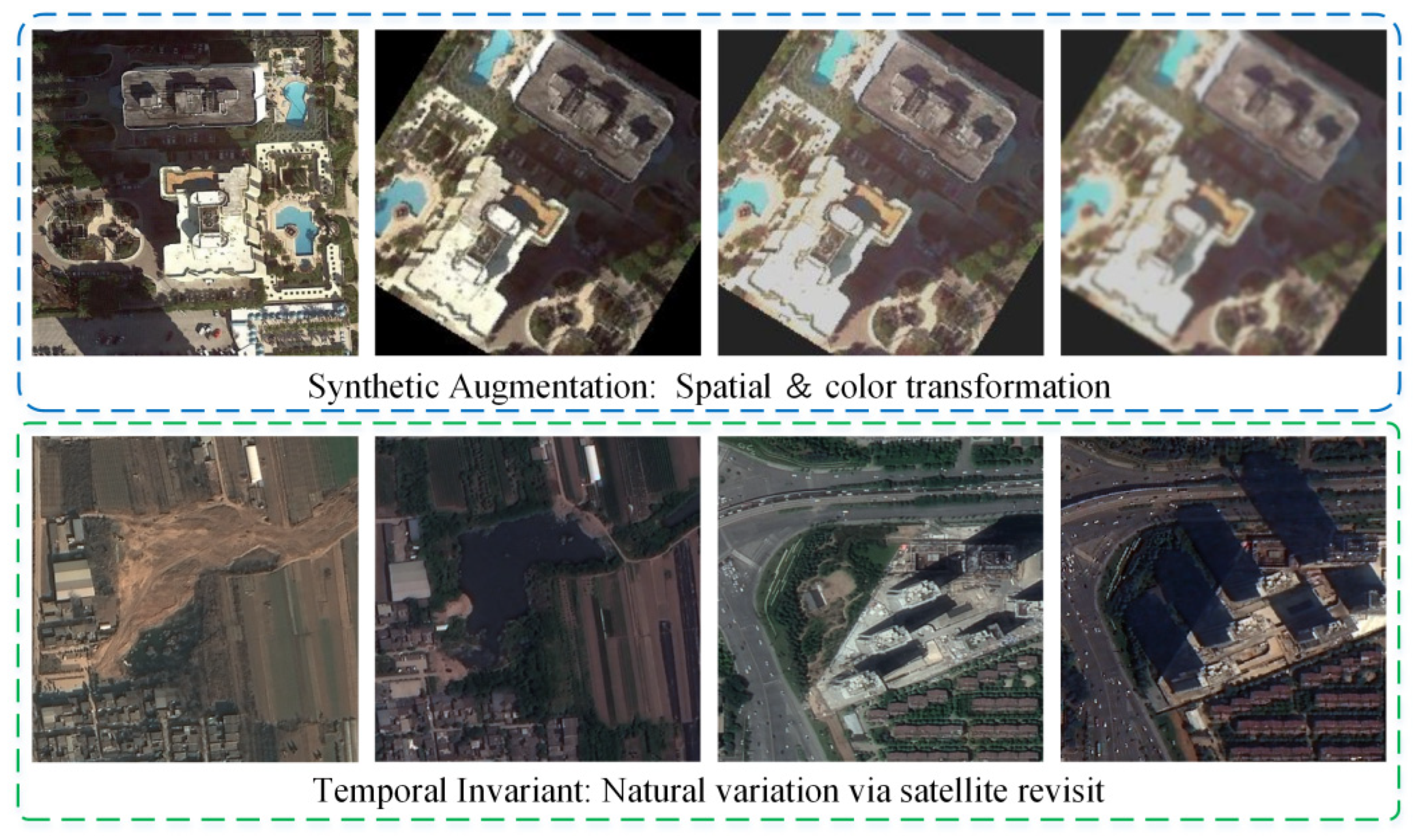
A unique characteristic of remote sensing data is the satellite revisit capability, which provides natural multi-temporal variations [24] (e.g., seasonal and illumination changes) that synthetic augmentations cannot replicate, as shown in Figure 1. SeCo [25] and SSL4EO-S12 [26] have exploited such temporal signals for self-supervision. A cross-temporal superpixel mask strategy [27] has further extended this idea to MIM. Multi-temporal imagery, thus, proves beneficial for tasks insensitive to temporal changes, such as scene classification, building and road detection [28]. Nevertheless, these methods predominantly treat multi-temporal images merely as additional positive views for invariance learning. This leaves a question: how can temporal signals be leveraged as a strategic instrument to suppress shortcut local cues and enforce scene-level reasoning?

Based on the above observation, we propose a self-supervised learning paradigm that exploits multi-temporal satellite revisits to capture scene-level semantic invariance. For pseudo-label construction, we collect a large set of long-interval satellite revisit images and process them with pixel-level registration. The SIFT inliers retained during registration serve as saliency priors to guide asymmetric masking across temporal views. Specifically, we construct three groups of positive pairs with progressively increasing difficulty: temporal-only variations (Pos₁), temporal variations with SIFT-guided asymmetric masking (Pos₂), and temporal variations with strong augmentations (Pos₃). This construction strategy compels the model to perform cross-view contextual reasoning rather than relying on pixel-wise correspondences. For the SSL framework, we propose MTC-Net, which integrates a progressive contrastive learning strategy with a dual-attention mechanism. Unlike standard contrastive methods that apply a single alignment objective at the final layer, our approach introduces layer-wise contrastive losses across stages. Further, we embed a dual-attention module that consists of spatial and channel attention to enhance the discriminability of intermediate features, with auxiliary losses that penalize attention on salient regions and enforce channel activation consistency across positive pairs. The pre-trained backbone is transferred to downstream RSSC tasks and evaluated on the AID [29], NWPU-RESISC45 [5], and UC Merced [30] datasets under limited-label settings. Our experimental results demonstrate that MTC-Net achieves competitive classification accuracy against state-of-the-art methods. The contributions can be summarized as follows:

• We introduce a self-supervised learning approach, MTC-Net, to improve remote sensing scene classification accuracy under insufficient annotated data.
• We leverage long-interval satellite revisit imagery to construct pseudo-labels, generating scene-consistent sample pairs that exhibit object-level variations.
• We design a progressive layer-wise contrastive learning framework that establishes a smooth curriculum from texture robustness to semantic invariance. We embed a dual-attention module with gated fusion and auxiliary losses to recalibrate intermediate features and enhance discriminability.

The remainder of this paper is organized as follows. Section 2 reviews related works. Section 3 provides a detailed description of the proposed method. Section 4 presents the experimental study results. Section 5 concludes the paper.

2. Related Works

2.1. Remote Sensing Scene Classification

The remote sensing scene classification task plays an important role in remote sensing image interpretation, having evolved in recent years from hand-crafted features to machine learning and deep learning approaches. Early studies focused on extracting hand-crafted features from RSIs, such as Scale Invariant Feature Transform (SIFT) [31], Local Binary Pattern (LBP), and Histogram of Oriented Gradients (HOG) [32]. These low-level visual features have strong statistical simplicity and interpretability, but are limited in capturing semantic information within complex scenarios. Methods for obtaining mid-level visual features, such as the Bag-of-Visual-Words model [33], Spatial Pyramid Matching (SPM), and Vectors of Locally Aggregated Descriptors (VLAD) [34], encode or aggregate low-level features to generate more discriminative feature representations. However, these approaches suffer from overly complex processing pipelines and heavy reliance on hand-crafted feature engineering.

With the rapid development of deep learning, researchers have begun to utilize its high-level semantic feature extraction capability in RSSC tasks. A series of deep neural networks proposed in recent years have achieved remarkable results in this field. For instance, MG-CAP [35] mitigated the semantic–visual discrepancy in RSIs through multi-granularity feature extraction and Gaussian covariance matrix normalization. CGINet [36] learned discriminative local features by incorporating context-aware global features. MBFNet [37] integrated a parallel convolution–Transformer backbone with kernel-selective multi-scale aggregation and a learnable multi-level fusion module. The work of MSCT [38] fused CNN and Transformer backbones via feature pyramid, channel attention, and cross-scale representation modules to boost RSSC performance. AF²-MSA Net [39] improved scene classification by combining multi-level feature extraction and an axis-aligned attention fusion mechanism. While the aforementioned works have advanced RSSC from diverse perspectives, the scarcity of annotated data remains one of the primary bottlenecks limiting the development of deep learning methods.

2.2. Self-Supervised Learning for Remote Sensing Images

Recently, self-supervised learning (SSL) has emerged as a prominent paradigm in deep learning. Different from supervised learning, self-supervised learning obtains the supervision signals from data itself through pretext tasks, enabling representation learning without manual annotations. A number of SSL methods have been tailored to remote sensing imagery. SCL-MLNet [40] incorporated self-supervised contrastive learning into the few-shot classification framework through multi-task learning, allowing the feature extractor to learn discriminative features from limited-labeled samples. SeCo [25] leveraged temporal and positional invariance to learn transferable representations from unlabeled time-series RSIs. MHCL [41] established an unsupervised contrastive learning approach that creates diverse queues through a hard feature transformation method, thereby enriching limited scene information and enabling the model to learn sufficient invariant representations. MGS-Net [42] combined background information with a self-guidance strategy; by strengthening the consistency of intra-class features, it effectively enhances classification performance. MPFASS-Net [18] introduced a progressive feature aggregation network based on Mamba and self-supervised learning, which alleviates the semantic gap in remote sensing images through cross-layer attention with Mamba fusion, class-center self-supervised learning, and decision-level feature integration.

2.3. Contrastive Learning for Remote Sensing Images

The core idea of contrastive learning is to attract positive pairs and repel negative pairs. Classic instance-wise contrastive learning methods include MoCo-v2 [43], SimCLR [44], BYOL [45], and SimSiam [46]. In the remote sensing domain, Lite-SRL [47] provided a lightweight representation learning method based on the SimSiam network, which effectively reduces computational load while maintaining high classification accuracy with a lightweight model architecture. MMPC-Net [17] introduced a multi-granularity and multi-scale progressive contrastive learning approach that guides a model to learn subtle details in remote sensing images by extracting features at different granularities across multiple stages. ViT-CL [48] combined a ViT model with supervised contrastive learning and jointly optimized cross-entropy and SupCon losses in a two-stage training strategy, improving both the accuracy and robustness of scene classification. CVT-SimCLR [49] presented a satellite image classification framework that integrates contrastive learning with CRF post-processing and cross-modal fusion.

2.4. Masked Image Modeling for Remote Sensing Images

Masked image modeling (MIM) has emerged as a powerful alternative to contrastive learning, where representations are learned by reconstructing randomly masked image patches or spectral bands. A systematic evaluation of MIM-pretrained vision transformers for RSSC [50] demonstrated that they significantly outperform supervised pretraining counterparts. RingMO [19] leveraged masked modeling to learn generalizable representations for remote sensing imagery. SatMAE [20] provided an MIM pretraining framework that utilized temporal multispectral satellite imagery and encoded different spectral band groups independently via spectral positional encoding, thereby better modeling spectral information and improving remote sensing representation learning. CMID [21] introduced a self-distillation framework that combines contrastive learning with masked modeling to balance global semantics and local details, enabling unified multi-level representation learning. CtxMIM [22] established a context-enhanced masked image modeling method that employs reconstruction consistency constraints to effectively capture semantic information in complex remote sensing scenes, significantly boosting self-supervised representation learning performance. BIMIM [23] presented a self-supervised learning framework for multispectral remote sensing imagery, which performs per-band independent masking and band-specific feature modeling to achieve fine-grained spectral information extraction and efficient cross-band learning.

3. Methods and Materials

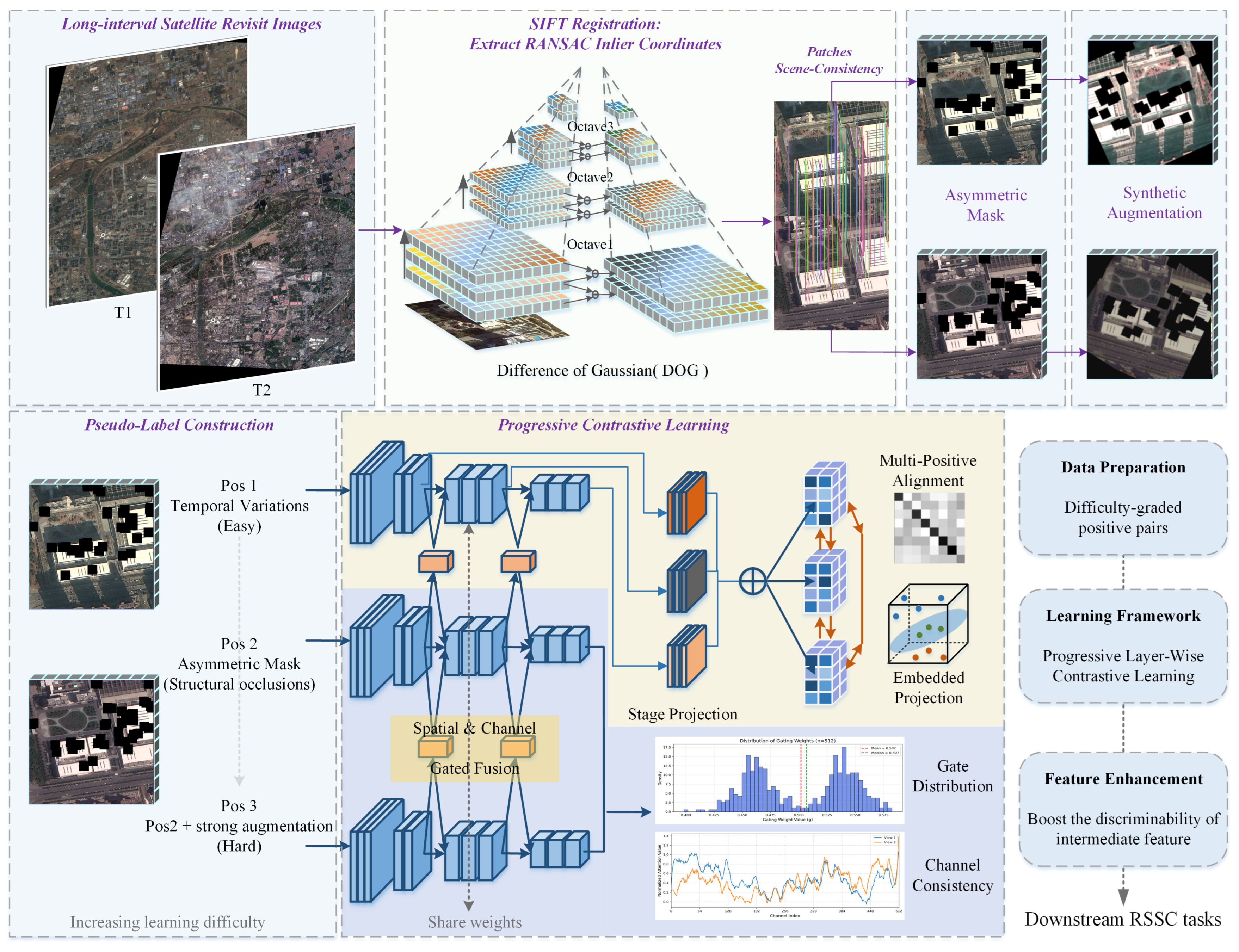
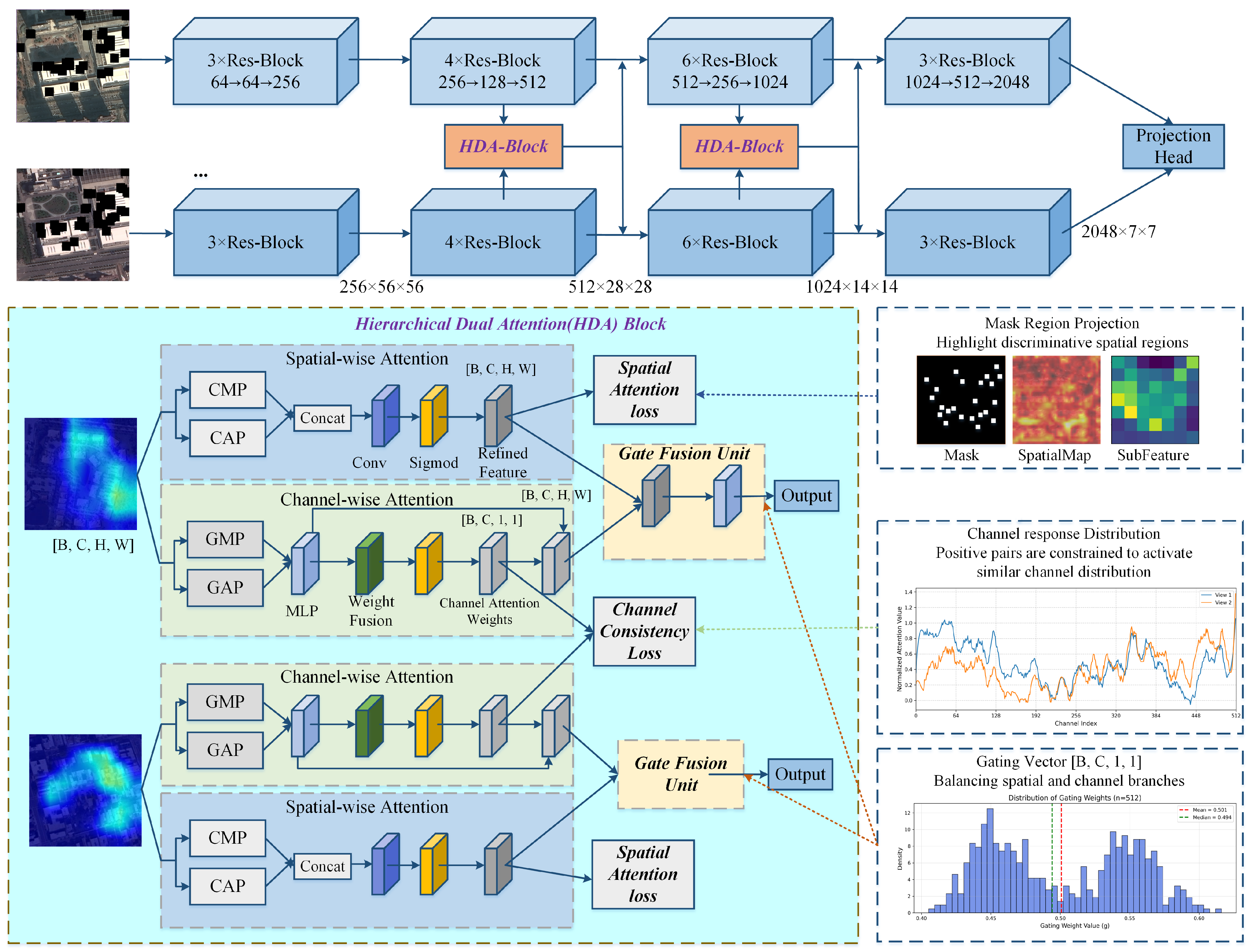
In this section, we present the proposed MTC-Net for the RSSC task, with its overall architecture illustrated in Figure 2. The core idea is to exploit the inherent tension between scene-level invariance and object-level variability in multi-temporal remote sensing images. This design compels the model to shift from local object memorization to global scene reasoning. The MTC-Net framework integrates a weight-sharing backbone with a progressive layer-wise contrastive loss and a dual-attention module, jointly learning discriminative scene representations from the constructed pseudo-labels.

3.1. Asymmetric Masking Across Temporal Views

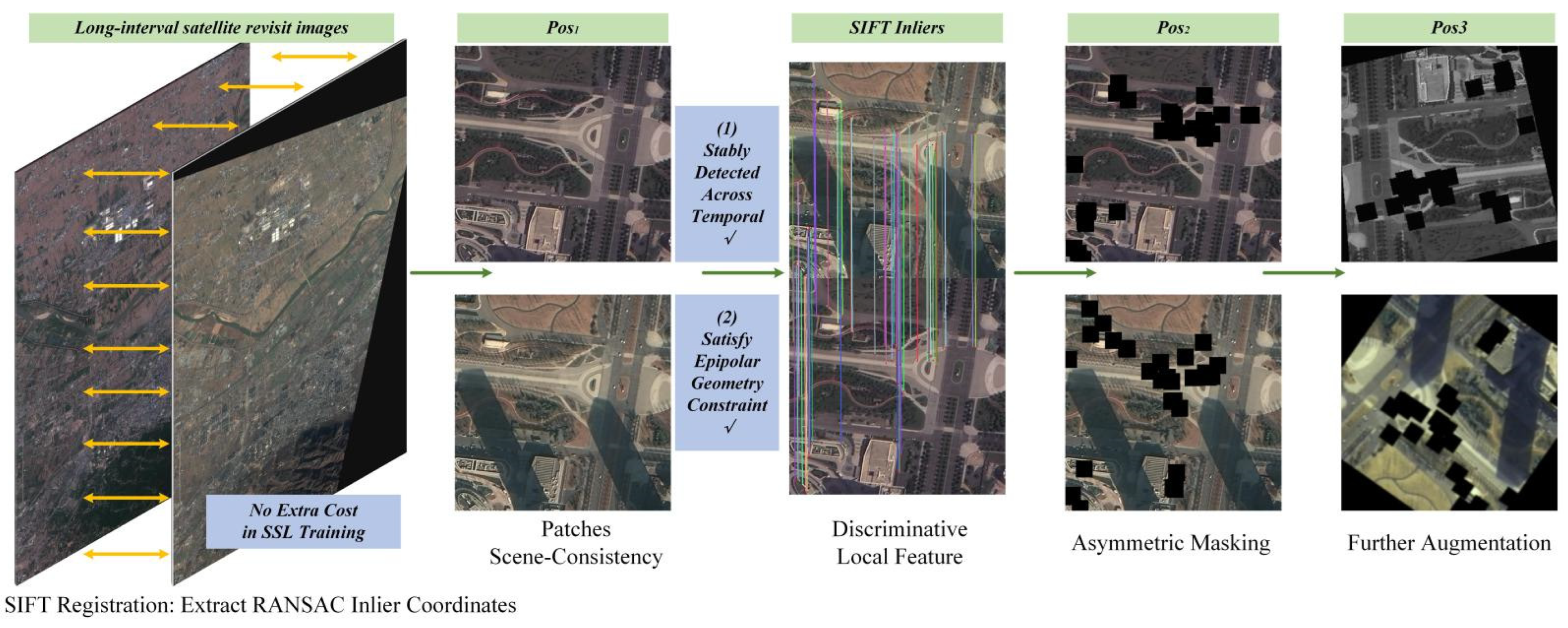
This section presents our proposed feature masking strategy, which exploits SIFT registration priors from multi-temporal RSIs to apply asymmetric local masking across the temporal views, as shown in Figure 3. This design compels the model to rely on global scene layout information during contrastive learning to determine that “this is the same scene,” rather than depending on pixel-level correspondences.

We utilized optical remote sensing images with sub-meter resolution provided by the Jilin-1 satellite constellations and the SuperView-1 satellite constellations. To ensure that satellite images of the same area captured natural variation, we controlled the satellite revisit intervals to a minimum of 2 months and a maximum exceeding one year. The collected dataset encompasses multiple scenarios, including artificial facilities, urban areas, aquatic areas, bare land, and vegetated regions.

Due to orbital variations, angular discrepancies, and perspective distortions, the coordinate projections of long-interval satellite images over the same region typically exhibit systematic biases. As a result, small-sized crops obtained based on geographic coordinates often contain inconsistent scene information. To address this issue, we rectified the spatial bias through SIFT-based pixel-level registration.

Local extreme points are detected as feature points using the Difference of Gaussian (DoG) method across temporal images I₁ and I₂:

$$\mathrm{D}\left(x,y,\sigma \right)=\left(G(x,y,k\sigma )-G(x,y,\sigma )\right)\ast I\left(x,y\right)$$

(1)

$$G\left(x,y,\sigma \right)={\displaystyle \frac{1}{2\pi {\sigma }^2}}{e}^{-{\displaystyle \frac{x^2+y^2}{2{\sigma }^2}}}$$

(2)

where I(x, y) represents the image at a specific scale, σ denotes the scale space factor, and k is the multiplicative factor between two adjacent scales, set $k=\sqrt{2}$. These key points, typically located at significant features like edges or corners, serve as anchors for generating feature descriptors. A 16 × 16-pixel window centered on each key point is divided into 4 × 4 sub-regions, and within each sub-region, the histogram for 8 directions of gradient is computed. The gradient amplitudes m(x, y) and gradient directions θ(x, y) are weighted by the following equations:

$$m\left(x,y\right)=\sqrt{{\left(I\left(x+1,y\right)-I\left(x-1,y\right)\right)}^2+{\left(I\left(x,y+1\right)-I\left(x,y-1\right)\right)}^2}$$

(3)

$$\theta \left(x,y\right)={\tan }^{-1}\left({\displaystyle \frac{I\left(x,y+1\right)-I\left(x,y-1\right)}{I\left(x+1,y\right)-I\left(x-1,y\right)}}\right)$$

(4)

For each key point, a 128-dimensional feature descriptor vector, structured as 4 × 4 × 8, is obtained. From image I₁, we extract feature descriptor vectors and form the set $D_1=\left\{k_{1i},d_{1i}\right\}$, where k_i denotes the spatial coordinates of the i-th key point and d_i is its corresponding 128-dimensional descriptor vector. For image I₂, we extract the set $D_2=\left\{k_{2i},d_{2i}\right\}$. The distance between each pair of feature points in D₁ and D₂ is calculated using the Euclidean distance, as shown in the following equation:

$$M_{i,j}=\sqrt{{\displaystyle \sum _{k=1}^{128}{\left(d_{1i}^k-d_{2j}^k\right)}^2}}$$

(5)

where $d_{1i}^k$ and $d_{2j}^k$ are the kth dimension components of the 128-dimensional vectors for the feature descriptor vectors. After this, matched feature points ${\left\{\left(q_i{,p}_i\right)\right\}}_{i=1}^N$ are derived by the Nearest Neighbor Distance Ratio (NNDR) matching method, where q_i, p_i are homogeneous coordinates in two images. To ensure geometric consistency, the RANSAC (Random Sample Consensus) algorithm is applied to filter out false matches. The objective is to maximize the cardinality of the inlier set that satisfies the epipolar constraint:

$$\hat{\mathrm{H}}=\mathrm{argmax}{\displaystyle \sum _{i=1}^{N}l\left({‖q_i-\mathrm{H}{p}_i‖}_2<\tau \right)}$$

(6)

where H denotes the estimated homography matrix and Hp_i denotes the projected coordinate of p_i under this transformation. The notation ‖‖₂ denotes the Euclidean distance, τ is the inlier distance threshold, and l(·) is the indicator function. The inliers retained after RANSAC filtering satisfy two conditions: (1) they can be stably detected in both temporal images, and (2) they satisfy the epipolar geometry constraint, meaning they physically correspond to the same ground object. Therefore, these SIFT inliers represent discriminative local features that persist across different time phases, ensuring that the masked regions are concentrated on high-frequency structures in the image.

The obtained geometrically verified inliers (RANSAC inliers) are used for image registration and also serve as the source of saliency priors for subsequent mask coordinate generation. The SIFT algorithm detects corners and edge regions with sharp intensity changes; these regions typically correspond to the most discriminative local structures within a scene. Furthermore, we adopt a cross-temporal misaligned masking strategy: by asymmetrically masking different salient regions on the two temporal slices, we break the model’s reliance on pixel-level correspondences and compel it to exploit global scene layout information to determine “this is the same scene.”

An excessively high masking ratio would disrupt too much of the scene structure. In the asymmetric masking process, for image A(T1), we randomly sample a subset of inliers M_A; for image B(T2), we randomly sample a subset M_B, where $M_A\cap M_B=\varnothing$. Centered at each selected inlier, we directly zero out pixels within its local neighborhood. This operation resembles patch masking in MIM, yet differs fundamentally: MIM randomly masks patches for reconstruction, whereas our saliency-guided masking targets discriminative local structures to compel the model toward global scene reasoning. Ablation experiments in Section 4 confirm that this cross-temporal asymmetric masking strategy yields superior performance.

We construct three groups of positive pairs with progressively increasing difficulty, as illustrated in Figure 4 and summarized in

Table 1. Positive sample pairs with progressively increasing dissimilarity.

Sample	Construction	Meaning	Difficulty
Pos1	Registered crops from different temporal	Temporal variations such as illumination, shadow, and seasonal differences	Low
Pos2	Pos1 + SIFT-guided asymmetric masking	Masking salient regions across views	Medium
Pos3	Pos2 + strong synthetic augmentations	Enhanced cross-view differences while preserving scene-level consistency	High

. The synthetic augmentation includes spatial transformations, Gaussian blur, color jitter, and random grayscale. Notably, we compute the SIFT priors during the registration stage and store the key point coordinates together with the first slice, so no additional computation is required during the self-supervised training stage.

3.2. Multi-View Synergistic Contrastive Learning

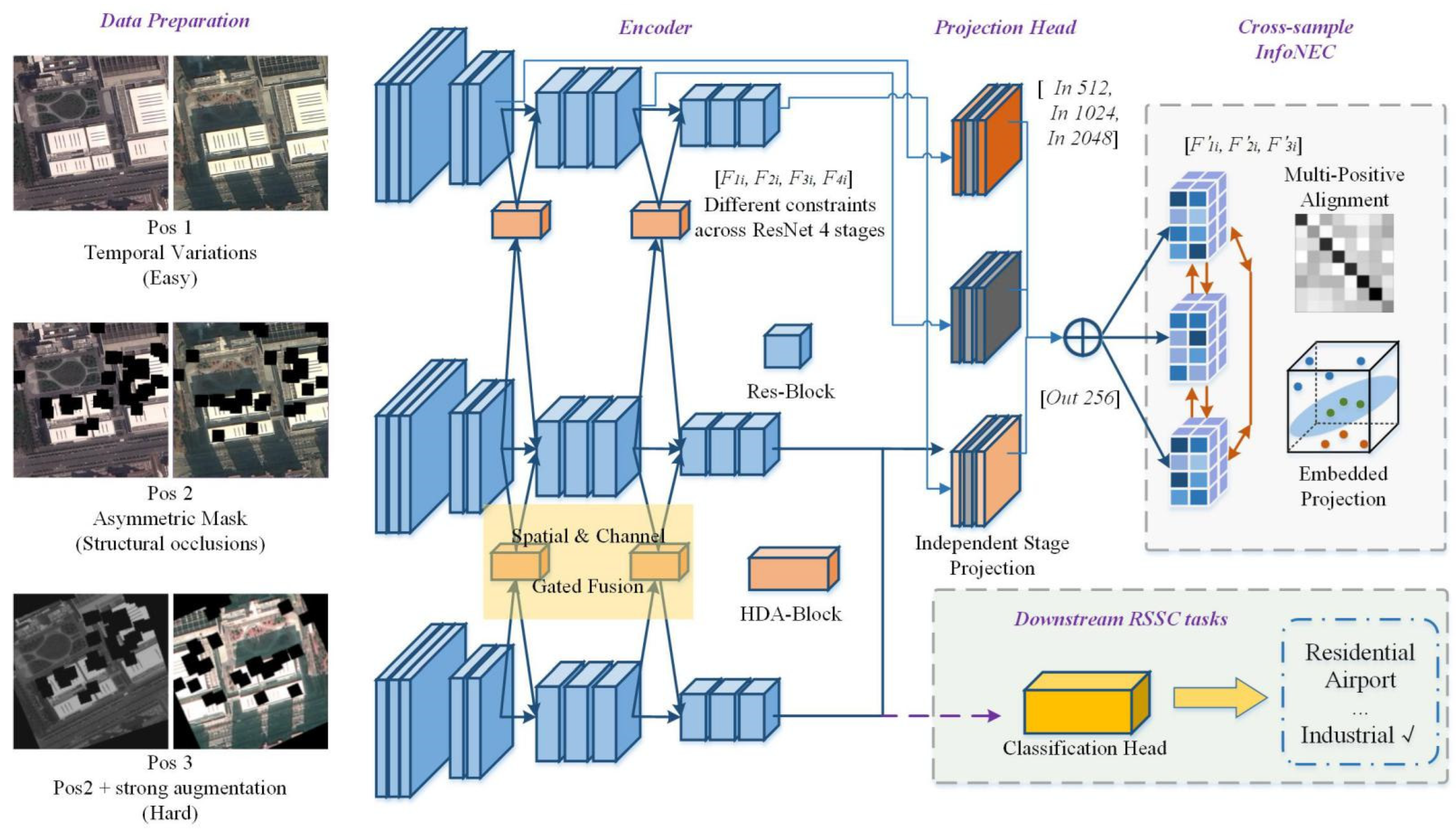
MTC-Net adopts a progressive contrastive learning strategy that guides the model from easy to hard by jointly leveraging the difficulty-progressive positive pairs constructed in Section 3.1 and layer-wise contrastive losses across network stages. We employ a weight-sharing mechanism and use ResNet-50 [51] as the weight-shared feature extractor. The successive stages of ResNet progressively encode representations from local textures to global semantics. Through the joint scheduling of data difficulty and network depth, we realize a structured curriculum learning scheme. The overall architecture is illustrated in Figure 5.

For each sample x within the sample set $\left\{x_1,x_2,\dots ,x_N\right\}$, three pairs of positive samples are generated through the pretext task, denoted as $\chi =\left\{\left(x_{t1}^1,x_{t2}^1\right),\left(x_{t1}^2,x_{t2}^2\right),\left(x_{t1}^3,x_{t2}^3\right)\right\}$. After being processed through the feature extractor f(·) and the projection head g(·), the resulting representations are L2-normalized according to the following equation:

$$z_t^i={\displaystyle \frac{g\left(f\left(x_t^i\right)\right)}{{‖g\left(f\left(x_t^i\right)\right)‖}_2}}$$

(7)

The objective of L2 normalization is to establish the equivalence between cosine similarity and the dot product. After processing through the feature extractor, the representation set $S=\left\{\left(z_{t1}^1,z_{t2}^1\right),\left(z_{t1}^2,z_{t2}^2\right),\left(z_{t1}^3,z_{t2}^3\right)\right\}$ is obtained. To strengthen the consistency constraint, all pairs $\left(z_{t1}^i,z_{t2}^j\right)\in S_{i,j}$ derived from T₁ and T₂ are designated as positive pairs. Meanwhile, representations from different instances within the same batch are constructed as negative pairs.

To impose differentiated constraints at varying depths, we attach independent lightweight projection heads after the last three ResNet stages; the output features from each stage are projected into a 256-dimensional contrastive space. Independent projection heads allow each layer to learn a mapping function that matches its own semantic granularity, so shallow and deep features are mapped into different subspaces.

$$Z_l^v={\mathit{ProjHead}}_l\left(F_l^v\right) l=[2,3,4]$$

(8)

where F_l^v denotes the feature map output by the l-th block of ResNet, with v ∈ {Pos₁, Pos₂, Pos₃} indicating the corresponding positive pair groups. At each layer, we compute the contrastive loss across the three groups of positive pairs, adopting a multi-positive InfoNCE formulation:

$$L_{\mathit{contrast}}^{\left(l\right)}=-{\displaystyle \frac{1}{B}}{\displaystyle \sum _{i=1}^B\log \frac{{\displaystyle {\sum }_{k=1}^3\exp \left(sim\left(Z_l^{{\mathit{pos}}_k,1},Z_l^{{\mathit{pos}}_k,2}\right)/{\tau }_l\right)}}{{\displaystyle {\sum }_{k=1}^3\exp \left(sim\left(Z_l^{{\mathit{pos}}_k,1},Z_l^{{\mathit{pos}}_k,2}\right)/{\tau }_l\right)}+{\displaystyle {\sum }_{j\ne i}\exp \left(sim\left(Z_l^{{\mathit{pos}}_k,1},Z_i^m\right)/{\tau }_l\right)}}}$$

(9)

where sim(u, v) represents the cosine similarity measurement function and τ_l is the temperature coefficient at layer l.

$$sim\left(u,v\right)={\displaystyle \frac{u^T\cdot v}{‖u‖\cdot ‖v‖}}$$

(10)

The overall contrastive loss is defined as the sum of the losses across all layers:

$$L_{\mathit{contrast}}={\displaystyle \sum _{l=1}^3{L}_{\mathit{contrast}}^{\left(l\right)}}$$

(11)

By optimizing the contrastive loss function, the primary objective is to minimize the distance between embeddings of positive pair samples while maximizing the distance between those of negative pairs. This enables the model to effectively discern scene consistency information. A selected subset proves sufficient to achieve adequate learning, as detailed in Section 4.4.

$$L_{\mathit{contrast}}=L\left(z_{t1}^{\mathit{pos}1},z_{t2}^{\mathit{pos}3}\right)+L\left(z_{t1}^{\mathit{pos}2},z_{t2}^{\mathit{pos}3}\right)+L\left(z_{t1}^{\mathit{pos}3},z_{t2}^{\mathit{pos}3}\right)$$

(12)

3.3. Dual-Attention Mechanism

This section introduces a dual-attention mechanism to enhance collaborative spatial and channel reasoning within the backbone. The effectiveness of layer-wise contrastive constraints ultimately hinges on feature quality. This mechanism adaptively highlights discriminative regions and channels, thus providing high-quality inputs for contrastive learning.

As shown in Figure 6, the dual-attention module is inserted after ResLayer2 and ResLayer3. This placement is motivated by the fact that lower-level features are too localized, while higher-level features lack sufficient resolution for effective spatial attention reconstruction.

The spatial attention branch is designed to localize the most discriminative spatial regions in a scene. During training, the locations of the masked regions are known in advance. This enables the generation of binary mask maps, where masked pixels are assigned 1 and unmasked pixels are assigned 0. To align the masked regions with the feature maps of Layer2 and Layer3, the binary masks are downsampled to 28 × 28 and 14 × 14 resolutions, respectively. Given their binary nature, max pooling is used to preserve the masked regions in the downsampled feature maps.

The resulting spatial attention map is normalized to the range [0, 1] via a sigmoid function and is trained to focus on masked regions. Since SIFT-based masks cover only a small area of the image, we adopt a weighted MSE loss that assigns higher weights to masked pixels. This encourages the model to assign higher attention weights to masked areas and lower weights elsewhere, thereby helping to recover important contextual information more effectively.

The ideal weight distribution $W_{s,ideal}^{(l)}$ and spatial attention loss are defined as follows:

$$W_{s,ideal}^{(l)}=\left\{\begin{array}{l}0.8,M^{(l)}(i,j)=1\\ 0.2,M^{(l)}(i,j)=0\end{array}\right.$$

(13)

$$L_{recon}^{(l)}={\displaystyle \frac{1}{H_l\cdot H_l}}{\displaystyle \sum _{i=1}^{H_l}{\displaystyle \sum _{j=1}^{H_l}{\left(W_s^{(l)}(i,j)-W_{s,ideal}^{(l)}(i,j)\right)}^2}}$$

(14)

The channel attention branch recalibrates channel weights to strengthen semantically discriminative features. Since all temporal views of the same scene (Pos₁, Pos₂, Pos₃) share the same semantic category, they should employ similar channel selection strategies. To this end, a channel consistency loss is imposed to enforce consistency between the channel attention vectors of each positive pair.

$$W_c^{(l)}=\sigma \left(w_d\cdot \mathrm{GAP}(X^{(l)})+w_d\cdot \delta (\mathrm{GMP}(X^{(l)})\right)$$

(15)

$$L_{consist}^{(l)}={\displaystyle \frac{1}{C_l}}{\displaystyle \sum _{c=1}^{C_l}{\left(w_c^{(l,view1)}(c)-w_c^{(l,view2)}(c)\right)}^2}$$

(16)

where X^l denotes the input features for layer l, σ represents the sigmoid activation function, GMP refers to Global Max Pooling, and GAP refers to global average pooling. W_c^I(1) and W_c^I(2) correspond to channel weights for different augmented views. Since the contrastive loss already handles negative separation, the channel attention loss is applied only to positive pairs. Imposing additional inconsistency on negative pairs would lead to over-constraint and training instability. The channel attention map is a weight vector with a size of 512 × 1 × 1, which is then broadcast to a feature map with a size of 512 × 28 × 28, matching the spatial dimensions of the spatial attention branch described above. This ensures the feasibility of subsequent gated feature fusion.

The gated fusion unit G dynamically adjusts the contributions of the spatial and channel attention branches based on scene content. The outputs of the two branches are first concatenated along the channel dimension, followed by global average pooling to aggregate global context. A multi-layer perceptron then generates a channel-wise gating weight vector g:

$${\mathrm{X}}_{\mathit{cat}}=\left[{\mathrm{X}}_{\mathit{spa}};{\mathrm{X}}_{\mathit{cha}}\right]\in {\mathbf{R}}^{2C\times H\times W}$$

(17)

$$g=\sigma \left(\mathit{MLP}\left(\mathit{GAP}\left[X_{\mathit{cat}}\right]\right)\right)\in {\mathbf{R}}^C$$

(18)

where σ denotes the sigmoid function. The final fused feature is a weighted combination of the two branches:

$$X_{\mathit{gated}}=g\cdot X_{\mathit{spa}}+\left(1-g\right)\cdot X_{\mathit{cha}}\in R^{C\times H\times W}$$

(19)

The additional parameters introduced by the dual-attention module primarily come from three sources: the channel MLP (approximately 2C² parameters), the spatial convolutional layers, and the gated fusion MLP (approximately 6C² parameters). For Layer2, where C = 512, this amounts to approximately 0.13 M parameters, accounting for only 0.15% of the total parameters of ResNet-50. In practice, the computational overhead of this module is negligible.

The total pre-training loss is a weighted sum of three loss terms. Based on the numerical magnitudes of the individual losses, the weighting coefficients are set to α = 0.1 for the spatial attention loss and β = 0.5 for the channel consistency loss.

$$L_{\mathit{total}}=L_{\mathit{contrast}}+\alpha L_{\mathit{recon}}+\beta L_{\mathit{consist}}$$

(20)

4. Experimental Study

4.1. Datasets and Implementation Details

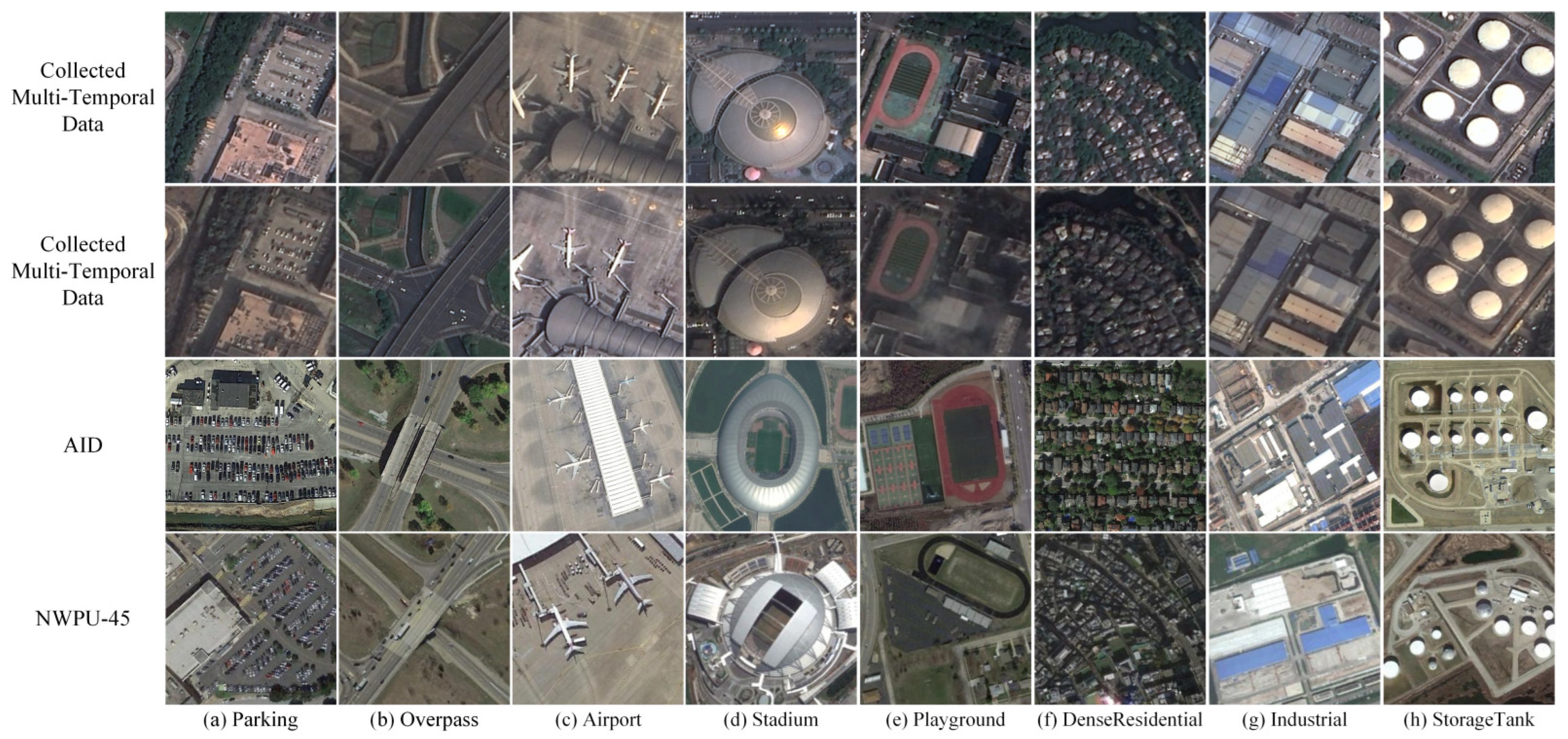
We evaluate our method on three widely used remote sensing scene classification datasets: NWPU-RESISC45 [5], AID [29], and UC Merced [30]. Sample images from these datasets, along with our multi-temporal data, are shown in Figure 7.

(i)

The NWPU-RESISC45 dataset, provided by Northwestern Polytechnical University, is a widely used open benchmark dataset for scene classification tasks. It consists of 45 scene categories, with each category containing 700 images sized 256 × 256 pixels. The spatial resolution of these images ranges from 0.5 to 30 m. The dataset is split into training and testing sets with ratios of 10:90 and 20:80, respectively.

(ii)

The Aerial Image dataset (AID) is a widely used aerial image dataset provided by the Wuhan University, consisting of 30 scene categories. Each category contains approximately 200 to 400 images, each with a size of 600 × 600 pixels. The dataset is split into training and testing sets with ratios of 20:80 and 50:50, respectively

(iii)

The UC Merced (UCM) dataset is sourced from the USGS National Map Urban Area Imagery collection, released by the UC Merced computer vision laboratory. It consists of 21 categories, with each category containing 100 images sized 256 × 256 pixels. The dataset is split into training and testing sets with ratios of 50:50 and 80:20, respectively. Detailed characteristics of these datasets are provided in

Table 2. Information on the datasets.

Datasets	Categories Number	Images Per Class	Image Count	Spatial Resolution	Crops Size	Training Rations (TR)
NWPU-RESISC45	45	700	31,500	0.5–30 m	256 × 256	10%, 20%
AID	30	200–400	10,000	0.8 m	600 × 600	20%, 50%
UC Merced	21	100	2100	0.3 m	256 × 256	50%, 80%

.

The self-supervised training used the stochastic gradient descent (SGD) optimizer with a momentum of 0.9, weight decay of 1 × 10⁻⁴, initial learning rate of 0.01, input size of 224 × 224, and batch size of 64. The learning rate scheduling utilized cosine annealing decay, and training was carried out for 200 epochs. The fine-tuning and linear probing evaluation used the Adam optimizer with a weight decay of 5 × 10⁻⁵, batch size of 64, input size of 224 × 224, and training for 100 epochs. For the classification head, the learning rate was 0.01, and in the fine-tuning test, the learning rate for the encoder was 1 × 10⁻⁵. All the experiments were implemented on two NVIDIA Tesla V100 GPUs.

4.2. Scene Classification

Following the aforementioned pretext task and self-supervised training, the model performance is evaluated on the scene classification task through both fine-tuning and linear probing evaluation. The parameters of the ResNet50 encoder are extracted and integrated with a fully connected layer of 2048 dimensions. This fully connected layer is denoted as the classification head C(·).

During the linear probing evaluation, also referred to as the freeze test, the parameters of the pre-trained encoder remain fixed while gradient back-propagation is exclusively executed within the classification head C(·). The classification head is tasked with mapping the extracted features to the target categories. The dual-attention mechanism is retained during testing, producing a stable fusion of the two attention branches.

During the fine-tuning evaluation phase, the parameters of the pre-trained encoder f(·) can be updated with a reduced learning rate. This allows gradual adaptation to the new task while preserving knowledge from the original pre-trained model. Both evaluation methods employ the cross-entropy loss:

$$L_{CE}=-y\log C{\left(\overline{f}\left(x\right)\right)}_{\left(x,y\right)\in D}$$

(21)

where D denotes the downstream scene classification training samples and $\overline{f}\left(\cdot \right)$ denotes the fixed parameters of f(·) in the linear probing evaluation.

4.3. Comparative Study

To evaluate the scene classification performance of the proposed MTC-Net, we conduct comprehensive comparisons with various state-of-the-art methods. The participating methods can be roughly categorized into three groups: (i) dedicated supervised RSSC methods, including MG-CAP [35], CGINet [36], MSCT [38], MBFNet [37], MSCNet [52], and AF²-MSANet [39]; (ii) MIM-based self-supervised methods, including CAE [50], MAE [50], RingMO [19], CtxMIM [22], and CMID [21]; and (iii) other representative self-supervised methods, including MTL [16], SeCo [25], Lite-SRL [47], ViT-CL [48], MGS-Net [42], MMPC-Net [17], and MPFASS-Net [18]. The experimental results on the three datasets are reported separately as follows.

Table 3. Results of fine-tuning experiment on AID in terms of overall accuracy (%).

Method	Source and Year	AID		Params (M)	FLOPs (G)
		TR = 20%	TR = 50%
ResNet50-ImageNet	CVPR2016	91.34 ± 0.10	94.79 ± 0.12	26.1	4.13
MG-CAP (Sqrt-E)	TIP2020	93.34 ± 0.18	96.12 ± 0.12	-	-
CGINet	TGRS2024	95.35 ± 0.14	97.10 ± 0.24	26.15	4.14
MSCT	RS2025	93.28 ± 0.26	98.21 ± 0.39	22.92	15.78
MBFNet	TGRS2025	95.81 ± 0.13	97.08 ± 0.17	26.09	4.25
MSCNet	TGRS2025	95.86 ± 0.16	97.46 ± 0.12	-	-
AF2-MSANet	JSTARS2026	95.86 ± 0.13	97.52 ± 0.11	34.64	5.47
CAE	SPIE2023	-	97.5	86.6	17.6
MAE	SPIE2023	-	98	86.57	17.56
RingMO-Vit	TGRS2023	96.54	98.38	86.57	17.6
MTL + ResNet101	RS2020	93.67 ± 0.21	96.61 ± 0.19	44.55	7.6
Seco + ResNet50	ICCV2021	93.47	95.99	26.1	4.13
Lite-SRL	RS2022	94.82	95.78	12.82	2.1
MGS-Net	TGRS2023	95.46 ± 0.21	97.18 ± 0.16	-	-
Vit-CL	JSTARS2023	95.6	97.42	86.57	18.2
MMPC-Net + ResNet50	GRSL2024	95.38 ± 0.20	97.52 ± 0.13	26.2	4.3
MTC-Net (ours)		95.92 ± 0.09	97.86 ± 0.12	26.33	4.25

presents the fine-tuning experiments conducted on AID. Under training ratios of 20% and 50%, MTC-Net achieves accuracies of 95.92% and 97.86%, respectively. The results reveal several noteworthy trends. MIM-based methods built upon the ViT architecture (e.g., MAE, RingMO) consistently achieve the highest accuracy, surpassing even many fully supervised RSSC methods. However, this performance gain comes at the cost of significantly increased parameter counts and FLOPs; these methods require 3.1× more parameters and 4.3× more FLOPs than our ResNet50 backbone, which limits their practical applicability. Second, compared with the self-supervised methods in Group iii, MTC-Net achieves superior accuracy, outperforming SeCo and MMPC-Ne with the same ResNet-50 backbone. This improvement stems from our deliberate integration of saliency-guided masking into the contrastive learning framework, which forces the model to rely on global scene layout rather than local shortcuts. These results confirm the effectiveness of our progressive contrastive design.

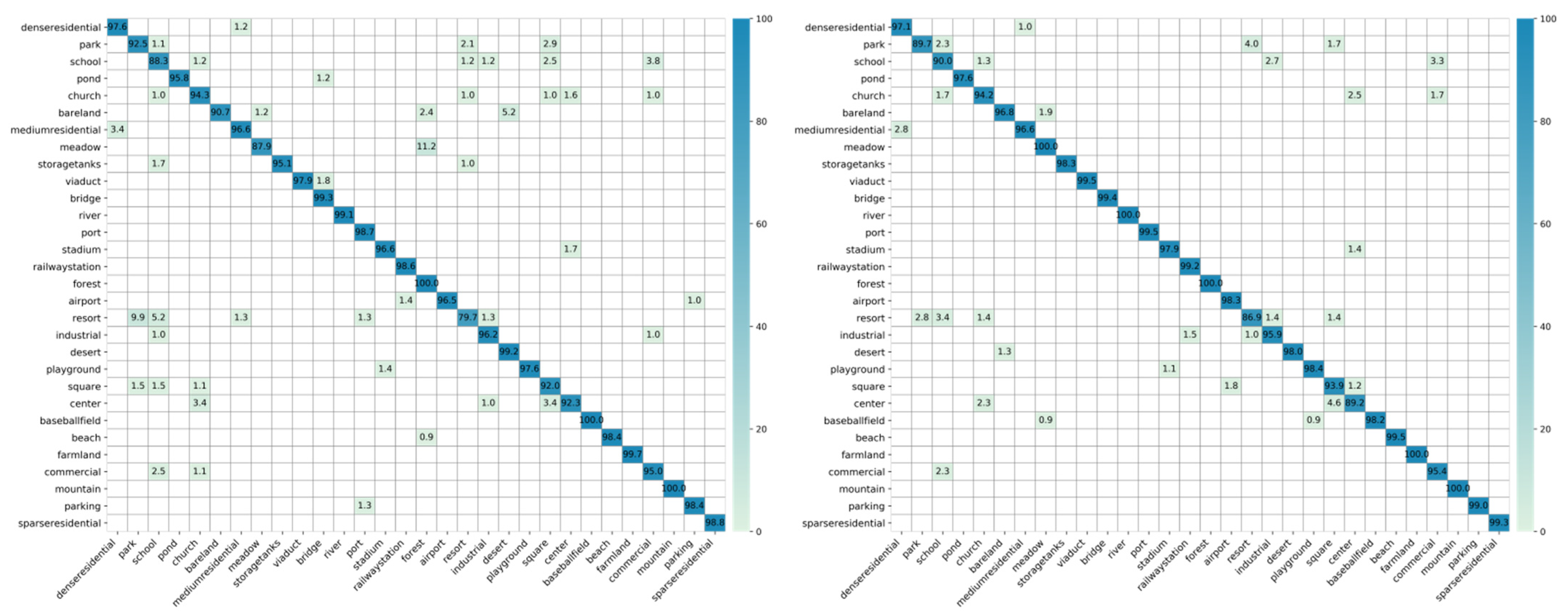
The confusion matrices for AID are presented in Figure 8. Under the 20% training condition, 23 of the 30 categories exceed 95% accuracy, with three reaching 100%. “Park” and “Resort” show relatively low accuracy: “School” is mainly misclassified as “Commercial,” and “Resort” as “Park.” Under the 50% condition, 25 categories exceed 95% accuracy, with six reaching 100%. “School” and “Resort” improve significantly, though “Resort” remains the least accurate due to its high visual similarity with other categories that also contain both buildings and vegetation.

Table 4. Results of fine-tuning experiment on NWPU-45 dataset in terms of overall accuracy (%).

Method	Source and Year	NWPU-45		Params (M)	FLOPs (G)
		TR = 10%	TR = 20%
ResNet50-ImageNet	CVPR2016	89.81 ± 0.08	92.24 ± 0.14	26.1	4.13
MG-CAP (Sqrt-E)	TIP2020	91.73 ± 0.18	93.49 ± 0.10	-	-
CGINet	TGRS2024	92.28 ± 0.17	94.38 ± 0.13	26.15	4.14
MSCT	RS2025	92.76 ± 0.13	93.67 ± 0.29	22.92	15.78
MBFNet	TGRS2025	-	-	26.09	4.25
MSCNet	TGRS2025	92.64 ± 0.09	94.59 ± 0.11	-	-
AF2-MSANet	JSTARS2026	92.8 ± 0.10	94.78 ± 0.13	34.64	5.47
CAE	SPIE2023	-	94.71	86.6	17.6
MAE	SPIE2023	-	94.4	86.57	17.56
RingMO-Vit	TGRS2023	93.46	95.35	86.57	17.6
CtxMIM (SWIN-B)	ACM2025	-	95.2	87.7	15.4
MTL + ResNet101	RS2020	91.61 ± 0.22	93.93 ± 0.16	44.55	7.6
Seco + ResNet50	ICCV2021	89.64	92.91	26.1	4.13
Lite-SRL	RS2022	92.77	93.51	12.82	2.1
Vit-CL	JSTARS2023	92.85	94.69	86.57	18.2
MGS-Net	TGRS2023	92.4 ± 0.16	94.57 ± 0.12	-	-
MMPC-Net	GRSL2024	92.75 ± 0.19	94.88 ± 0.15	26.2	4.3
MPFASS-Net	TGRS2025	93.12	94.93 ± 0.11	32.06	-
MTC-Net (ours)		93.16 ± 0.12	94.97 ± 0.08	26.33	4.25

presents the fine-tuning results on the NWPU-RESISC45 dataset at 10% and 20% training ratios. MTC-Net achieves accuracies of 93.16% and 94.97%, respectively. MIM-based methods again achieve the highest accuracy, even surpassing the fully supervised methods listed. Compared with the contrastive learning methods in Group iii, MTC-Net offers a highly competitive accuracy–efficiency trade-off for remote sensing scene classification, benefiting from the integration of saliency-guided masking into the contrastive learning framework. Despite having more categories and images than AID and UCM, NWPU-RESISC45 still sees encouraging classification performance from MTC-Net, further validating the effectiveness of our design.

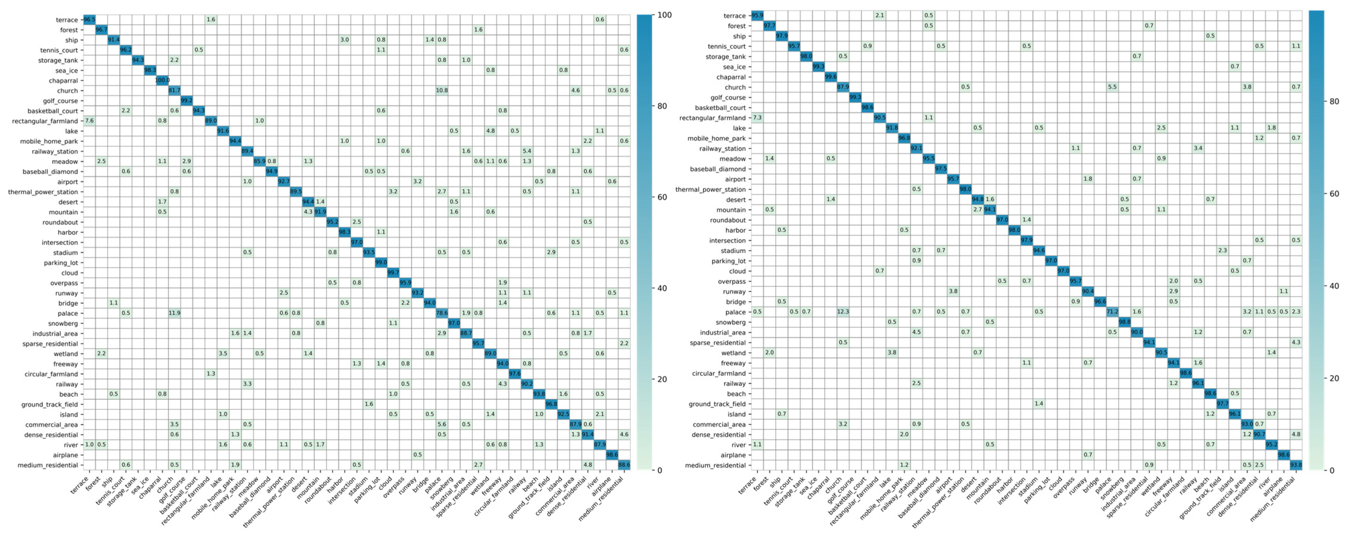
The confusion matrices for the NWPU-45 dataset are presented in Figure 9. At a 10% training ratio, 37 of the 45 categories exceed 90% accuracy. The lowest accuracies occur for “Church” and “Palace,” where “Church” is mainly misclassified as “Palace” and “Commercial Area” due to the similar architectural layouts shared among these artificial facilities. Some dispersed misclassifications are also observed, but this issue diminishes as training samples increase. Under the 20% condition, 43 categories exceed 90% accuracy. The confusion between “Church” and “Palace” persists despite the increased data, suggesting fundamental feature ambiguity rather than sample insufficiency.

Table 5. Results of fine-tuning experiment on UCM dataset in terms of overall accuracy (%).

Method	Source and Year	UCM
		TR = 50%	TR = 80%
ResNet50-ImageNet	CVPR2016	95.45	98.33
CGINet	TGRS2024	-	99.84 ± 0.14
MSCT	RS2025	98.97 ± 0.11	99.84 ± 0.16
MBFNet	TGRS2025	98.86 ± 0.11	99.76 ± 0.08
MSCNet	TGRS2025	99.26 ± 0.07	99.95 ± 0.10
AF2-MSANet	JSTARS2026	-	99.92 ± 0.10
CAE	SPIE2023	-	99.76
MAE	SPIE2023	-	99.76
RingMO-Vit	TGRS2023	-	99.46
CMID	TGRS2023	-	99.22
MTL + ResNet101	RS2020	-	99.02
Seco + ResNet50	ICCV2021	-	97.86
Lite-SRL	RS2022	98.67	99.76
Vit-CL	JSTARS2023	99.14	99.76
MGS-Net	TGRS2023	-	99.76 ± 0.14
MMPC-Net	GRSL2024	98.86 ± 0.17	99.76 ± 0.12
MPFASS-Net	TGRS2025	99.42 ± 0.15	99.84 ± 0.07
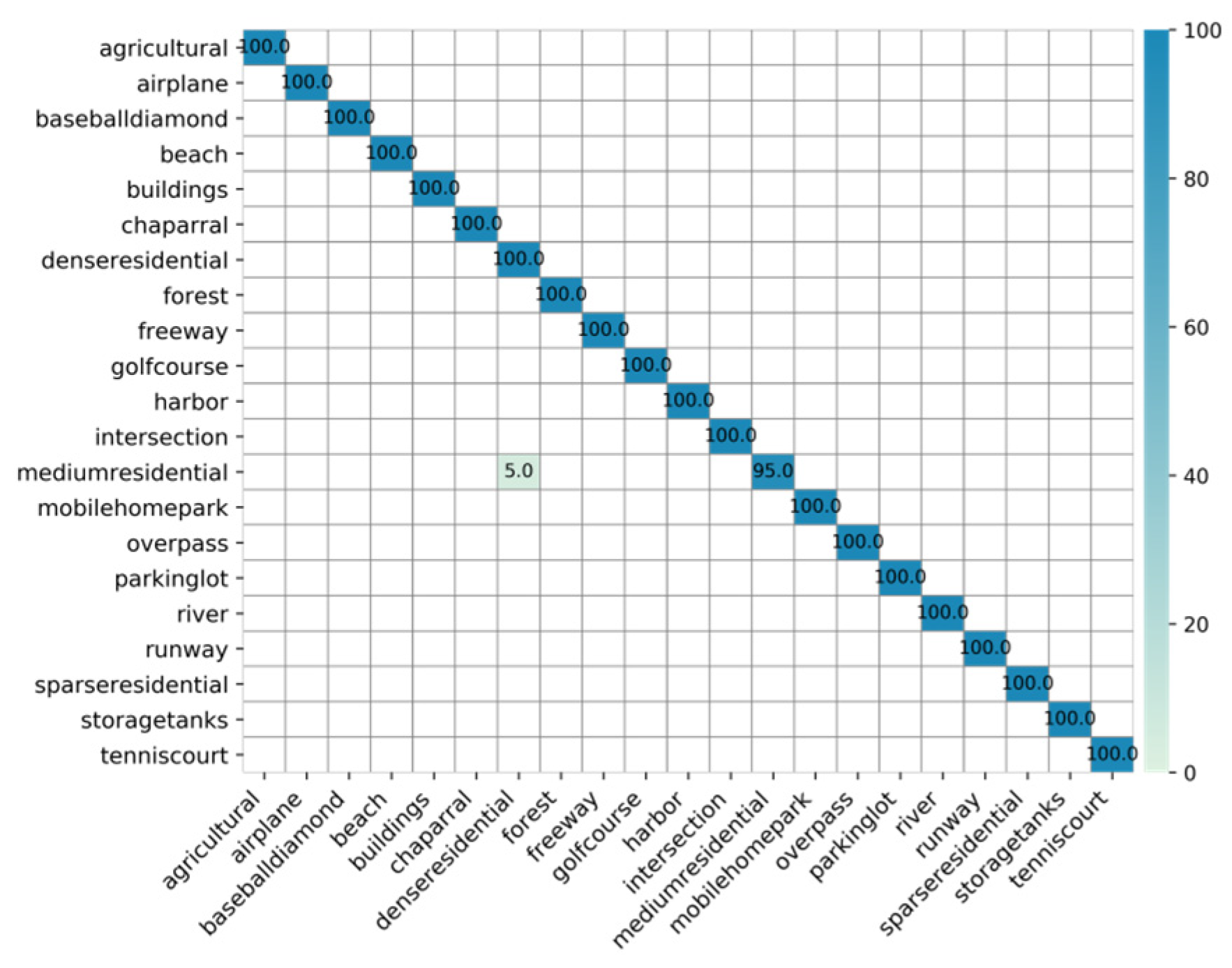
MTC-Net (ours)		99.26 ± 0.12	99.84 ± 0.05

presents the fine-tuning results on the UC Merced dataset at 50% and 80% training ratios. MTC-Net achieves accuracies of 99.26% and 99.84%, respectively. The results demonstrate that MTC-Net achieves effective classification performance on this dataset. The confusion matrices are presented in Figure 10. The dataset contains 21 categories, and the proposed method attains high overall accuracy. Notable confusion is observed between the “Medium Residential” and “Dense Residential” categories, primarily due to their similar spatial layouts and building densities.

Table 6. Results of linear probing experiment in terms of overall accuracy (%).

Method	AID	NWPU-45
	TR = 50%	TR = 20%
ImageNet Supervised	81.56	72.92
MOCO-v2	82.62	69.25
SimCLR	80.21	66.58
BYOL	67.95	57.34
SimSiam	78.92	63.81
SWAV	-	54.38
PCL	-	74.09
MHCL	-	78.80
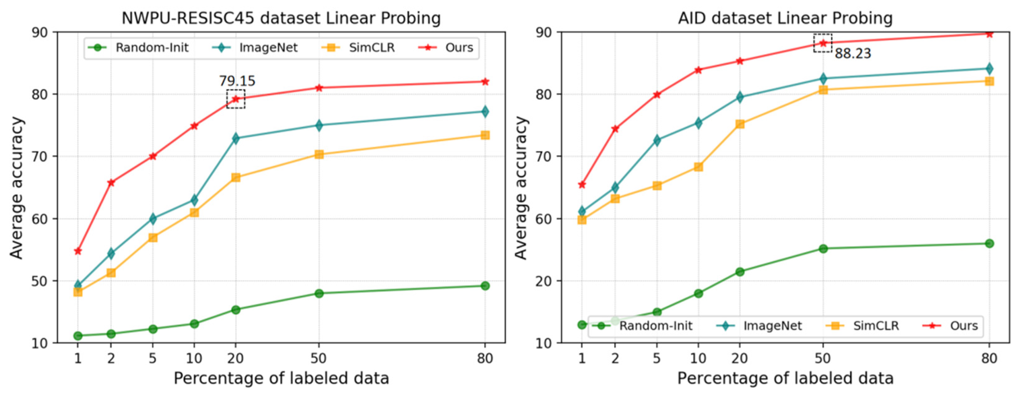
Ours	88.23	79.15

presents the results of the linear probing experiment; we compared MTC-Net with several instance-wise contrastive learning methods, including the classic approaches MoCo-v2 [43], SimCLR [44], BYOL [45], and SimSiam [46], as well as the clustering-based methods SWAV [53] and PCL [54]. The results indicate that despite the encoder being frozen, the model is capable of mapping features to the correct classification space. MTC-Net shows significant improvement over the Image-Net pre-trained model despite the vast disparity in dataset scale and differences in supervised information; this demonstrates that MTC-Net effectively learns latent representations from remote sensing data. Compared to classical contrastive learning methods, MTC-Net’s multi-temporal scene consistency and multi-view synergistic learning strategy significantly enhance the model’s representation extraction capabilities. Figure 11 illustrates the linear probing accuracy curve under increasing percentages of labeled data, with MTC-Net exhibiting a distinct advantage across all stages. Its performance rapidly increases within the 1–20% interval and gradually plateaus within the 20–80% interval. This occurs because linear probing training only updates the parameters of the last fully connected layer, and the final classification performance ultimately reflects the representation extraction capability of the encoder layer.

4.4. Visualization Results

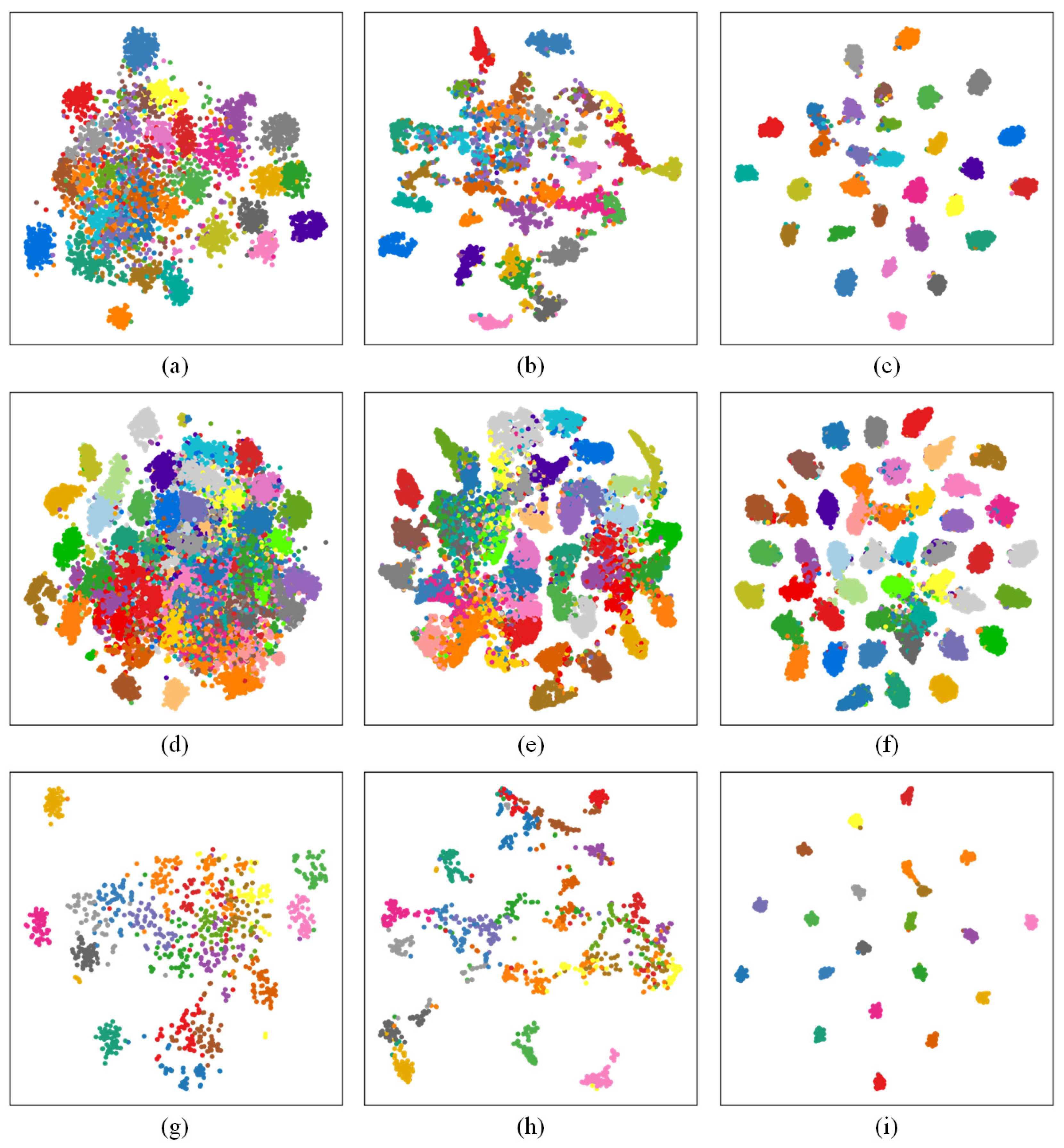
We employ t-SNE (t-Distributed Stochastic Neighbor Embedding) [55] to visualize the efficacy of the proposed method. For our pre-trained model, our fine-tuned model, and the ImageNet pre-trained model, the test set samples are each processed through the encoder to generate a 1 × 2048-dimensional vector. T-SNE projects all these high-dimensional vectors into a 2D space, with identical colors assigned to samples from the same category. As shown in Figure 12, after pre-training with our proposed framework, the encoder achieves better clustering performance. Thus, the proposed method can yield valuable scene consistency information for downstream RSSC tasks.

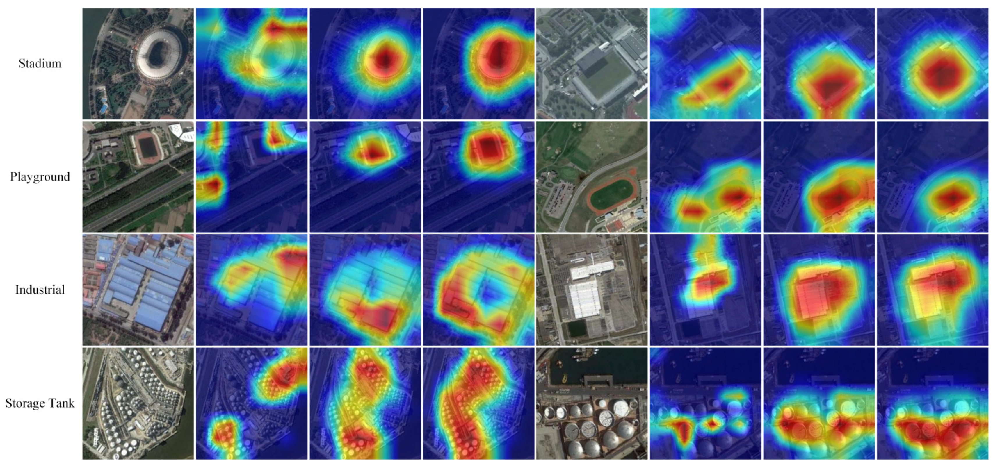
Furthermore, we implement Grad-CAM (Gradient Weighted Class Activation Mapping) [56] to visualize discriminative features of the pre-trained model. Within this framework, channel-wise importance weights are derived by applying global average pooling to the gradients of the target category with respect to the final convolutional layer’s feature map. These weights are then used to perform a weighted summation of the feature maps across channels, followed by ReLU activation to generate a class-specific activation heatmap. As shown in Figure 13, we compare the model pre-trained by MTC-Net, the fine-tuned model, and the ImageNet pre-trained model. Taking the “Stadium” as an example, which exhibits a distinct contour, the ImageNet pre-trained model demonstrates a dual focus on both the stadium area and other regions. The MTC-Net model exhibits a significant shift in attention, with a pronounced emphasis on the stadium area. The “Playground” category shares similar characteristics with “Stadium” but exhibits lower boundary clarity; the initial model exhibits misalignment in its attention region. After self-supervised training, the model demonstrates increased focus on the main ground region and achieves competitive performance relative to the fine-tuned model.

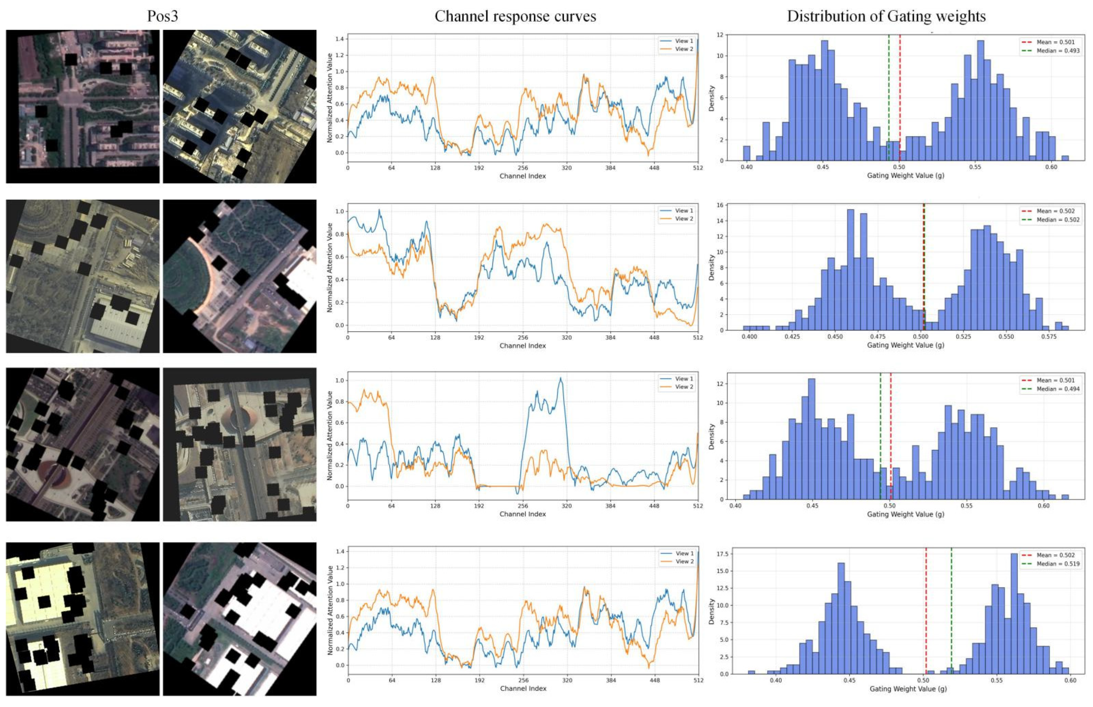
To illustrate channel consistency, we visualize the 512-dimensional channel attention weights of positive pairs as response curves, shown in the middle column of Figure 14. The vertical axis represents the normalized attention weights. Under the challenging Pos₃ condition, where both asymmetric masking and strong augmentations are applied, the overall fluctuation trends remain consistent. Meanwhile, channel activation patterns across different samples show significant divergence, confirming that this consistency is not globally uniform.

To validate the adaptive fusion strategy of the gated fusion unit G, we analyze its output gating vector g ∈ [0, 1]⁵¹², as shown in the right column of Figure 14. The horizontal axis represents the gating weight g and the vertical axis denotes the probability density. The histogram exhibits a clear bimodal distribution. g→0 indicates stronger reliance on channel attention, while g→1 reflects a preference for spatial attention. The weights do not collapse to zero or one, suggesting that the model retains complementary information from both branches. Furthermore, the notable variance across samples confirms that the gating module adapts its fusion strategy according to the scene content, rather than generating fixed weights.

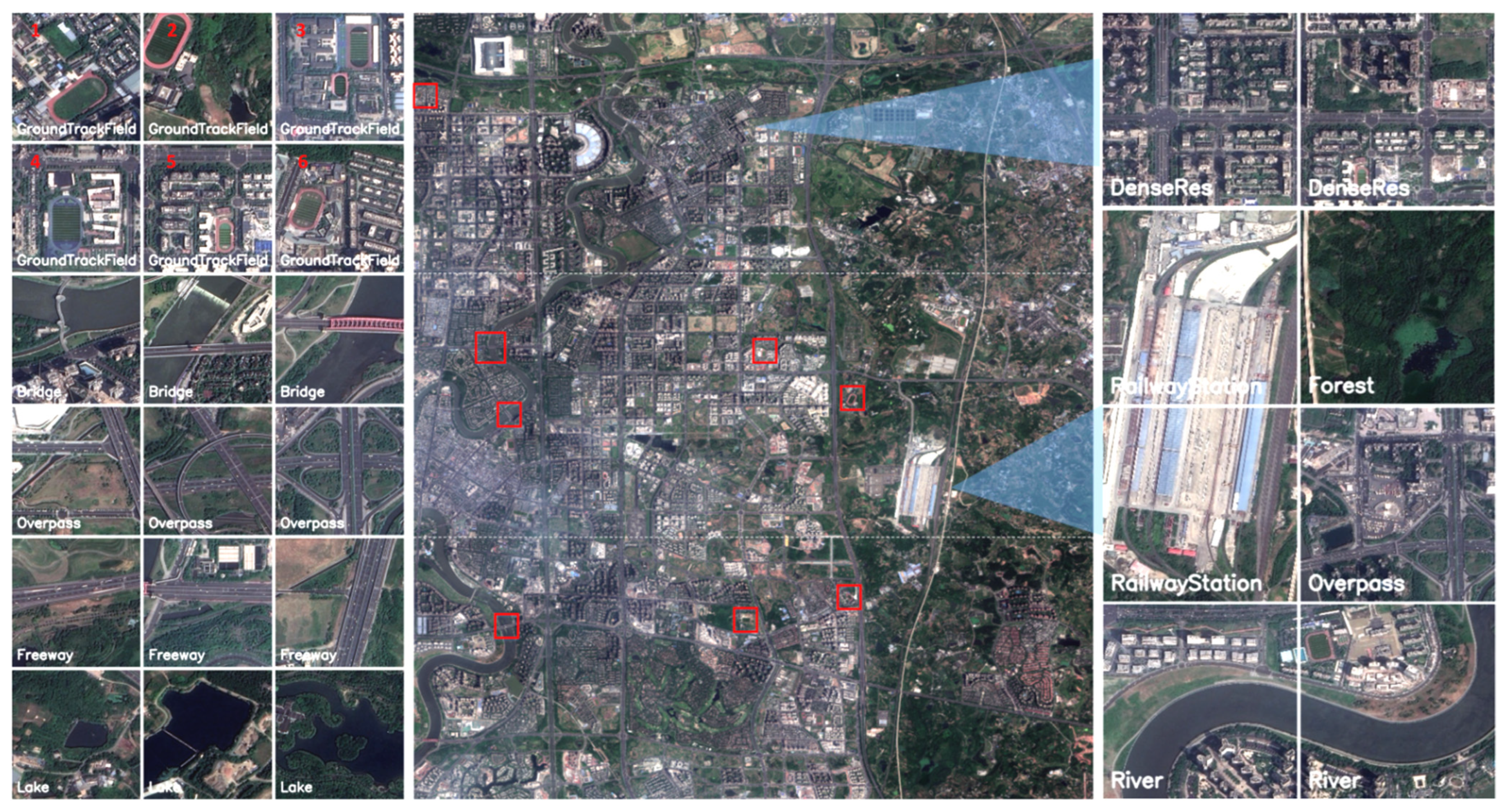
The sliding-window classification results on a large-scale RS image are shown in Figure 15. A fine-tuned MTC-Net model based on the NWPU-45 dataset is employed, and the evaluated large-scale images are selected from the urban scenes used in the self-supervised pretext task. After representation learning via MTC-Net and fine-tuning with a small amount of training data, the model can accurately pinpoint key landscape features, thereby enabling rapid localization of the target scenes to be searched. Based on these results, a customized model for a new scene classification task can be obtained by fine-tuning the pre-trained MTC-Net model with only a few annotated samples.

4.5. Ablation Study

We evaluated the effectiveness of each component in MTC-Net at the 20% training ratio of the NWPU-RESISC45 dataset.

Table 7. Results of different masking strategies in terms of overall accuracy (%).

Component	Overall Accuracy (%)
Synthetic *	94.10
Temporal	93.95
Randomly mask	94.45
Select identical feature points for mask	93.79
+ SIFT-guided asymmetric masking (blur)	94.82
+ SIFT-guided asymmetric masking	94.97

Synthetic * indicates generating positive pairs solely through synthetic augmentation, which represents the classic discriminative contrastive learning approach.

analyzes the impact of different masking strategies in the pretext task. Unlike standard masked image modeling, our approach does not involve pixel reconstruction; we directly employ the masked images as contrastive samples to learn invariant feature representations. This deliberate increase in optimization difficulty enhances model performance. When positive pairs are constructed solely from temporal changes, the model underperforms the classic discriminative contrastive learning method. This occurs because some land features remain unchanged across temporal images, resulting in minimal differences within positive pairs. Incorporating key point masking improves accuracy by 0.72%, indicating that each component contributes positively to the representation learning process. We also compare different masking operations. The zero-out pixel strategy outperforms blur-based masking by 0.17%. In contrast, masking identical feature points across both views leads to negative optimization. We attribute this to the fact that masking identical regions in sequential crops artificially simplifies the contrastive task, as the positive samples already share substantial overlapping visual information.

Table 8. Results of multiple combinations experiment in terms of overall accuracy (%).

Condition	$\mathit{l}\left({\mathit{z}}_{\mathit{t}1}^{\mathit{pos}1},{\mathit{z}}_{\mathit{t}2}^{\mathit{pos}3}\right)$	$\mathit{l}\left({\mathit{z}}_{\mathit{t}1}^{\mathit{pos}2},{\mathit{z}}_{\mathit{t}2}^{\mathit{pos}3}\right)$	$\mathit{l}\left({\mathit{z}}_{\mathit{t}1}^{\mathit{pos}3},{\mathit{z}}_{\mathit{t}2}^{\mathit{pos}3}\right)$	${\mathit{L}}_{\mathit{r}\mathit{e}\mathit{c}\mathit{o}\mathit{n}}^{(\mathit{l})}$	${\mathit{L}}_{\mathit{c}\mathit{o}\mathit{n}\mathit{s}\mathit{i}\mathit{s}\mathit{t}}^{(\mathit{l})}$	Gate	OA (%)
1	✓						94.32
2	✓		✓				94.64
3	✓	✓	✓				94.72
4	✓	✓	✓	✓		-	94.76
5	✓	✓	✓	✓	✓	Gated Fusion	94.97
6 *	-	-	-	-	-	Gated Fusion	94.98
7	✓	✓	✓	✓	✓	Summation	94.60

Condition 6 * indicates all combinations of $\left(z_{t1}^i,z_{t2}^j\right)$, which incurs large computational load.

analyzes the contributions of multiple combinations in multi-view synergy. Condition 3 refers to both T₁ and T₂ employing rotation and angular color transformations to induce substantial differences at the object level, which outperforms Conditions 1–2 by 0.40%. This result suggests that MTC-Net drives the model toward scene-consistent information during training. Removing the channel consistency loss in Condition 4 leads to a 0.21% decrease in accuracy, validating its critical role in maintaining temporally invariant feature selection. Condition 5 demonstrates that the dual-attention mechanism further improves accuracy by 0.27%. The spatial-wise $L_{recon}^{(l)}$ and the channel-wise $L_{consist}^{(l)}$ attention branches are jointly employed, alleviating the hierarchical feature information loss induced by the pseudo-label construction strategy. Conditions 5 and 6 differ by only 0.01% in accuracy, yet Condition 5 substantially reduces computational cost. Therefore, as defined in Equation (12), we demonstrate that the selected subset is sufficient to achieve effective learning outcomes. This dual confirmation underscores our framework’s ability to decouple scene semantics from object appearance variations. We further ablate the gated fusion unit by replacing it with fixed summation in Condition 7. This results in a 0.37% accuracy drop, confirming the benefit of gated fusion.

5. Conclusions

In this paper, we propose MTC-Net, a self-supervised learning framework for remote sensing scene classification that exploits multi-temporal satellite imagery to learn scene-level invariant representations without manual annotations. Our core idea is a saliency-guided asymmetric masking strategy, which uses SIFT inliers from cross-temporal registration as priors to remove discriminative local features, thereby forcing the model to shift from object memorization to global scene reasoning. To learn from these challenging positive pairs, we design a progressive layer-wise contrastive learning architecture that establishes a smooth curriculum from local texture robustness to global semantic invariance. A dual-attention module and a gated fusion unit are further introduced for adaptive feature recalibration.

Extensive experiments on three benchmark datasets, NWPU-RESISC45, AID, and UC Merced, under limited-label settings demonstrate that MTC-Net achieves superior accuracy compared with state-of-the-art methods. Ablation studies confirm the contribution of each component, while visualization analyses validate that the interplay between scene-level invariance and object-level ambiguity underpins the model’s strong generalization.

References

1. Chen, J.; Yi, J.; Chen, A.; Jin, Z. EFCOMFF-Net: A Multiscale Feature Fusion Architecture with Enhanced Feature Correlation for Remote Sensing Image Scene Classification. IEEE Trans. Geosci. Remote Sens. 2023, 61, 1–17. [Google Scholar] [CrossRef] [Scilit]
2. Wang, Y.; Shao, Z.; Xue, Z.; Yang, G.; Zhou, J.; Zuo, X. Lightweight remote sensing super-resolution with multi-scale graph attention network. Pattern Recognit. 2024, 154, 111178. [Google Scholar] [CrossRef] [Scilit]
3. Sun, B.; Yan, W.-D.; Zhang, T.; Ma, X.-L.; Bian, H.; Ni, W.-P. A New Remote Sensing Image Automated Registration Algorithm Based on Multi-Feature and Well-Distribution. Mod. Appl. Phys. 2012, 3, 339–346. [Google Scholar]
4. Yan, Y.; Wang, Y.; Tu, W.; Wang, J.; Cai, B.; Zhuang, Q.; Chen, Y.; Zhang, H.; Shao, Z. S3Mamba: Pan-Sharpening via Spatial–Spectral Synergistic State Space Model. IEEE J. Sel. Top. Appl. Earth Obs. Remote Sens. 2026, 19, 12820–12834. [Google Scholar] [CrossRef] [Scilit]
5. Cheng, G.; Han, J.; Lu, X. Remote Sensing Image Scene Classification: Benchmark and State of the Art. Proc. IEEE. 2018, 105, 1865–1883. [Google Scholar] [CrossRef] [Scilit]
6. Wu, J.; Li, B.; Qin, Y.; Ni, W.; Zhang, H.; Sun, Y. A Multiscale Graph Convolutional Network for Change Detection in Homogeneous and Heterogeneous Remote Sensing Images. Int. J. Appl. Earth Obs. Geoinf. 2021, 105, 102615. [Google Scholar] [CrossRef] [Scilit]
7. He, K.; Chen, X.; Xie, S.; Li, Y.; Dollár, P.; Girshick, R. Masked Autoencoders Are Scalable Vision Learners. In Proceedings of the IEEE/CVF Conference on Computer Vision and Pattern Recognition (CVPR), New Orleans, LA, USA, 18–24 June 2022; IEEE: New Orleans, LA, USA, 2022; pp. 15979–15988. [Google Scholar]
8. Liu, X.; Zhuang, Y.; Chen, H.; Zhang, X.; Li, L. Task-Driven Regional Saliency Analysis Based on a Global–Local Feature Assembly Network in Complex Optical Remote Sensing Scenes. IEEE Geosci. Remote Sens. Lett. 2020, 17, 1655–1659. [Google Scholar] [CrossRef] [Scilit]
9. Dong, C.L.; Zhang, Y.X.; Meng, X.; Guo, L.X. Application Evaluation of Simulated SAR Image for Target Recognition. Mod. Appl. Phys. 2025, 16, 266–272. [Google Scholar] [CrossRef] [Scilit]
10. Kolesnikov, A.; Zhai, X.; Beyer, L. Revisiting Self-Supervised Visual Representation Learning. In Proceedings of the IEEE/CVF Conference on Computer Vision and Pattern Recognition (CVPR), Long Beach, CA, USA, 15–19 June 2019; pp. 1920–1929. [Google Scholar]
11. Stojnić, V.; Risojević, V. Self-Supervised Learning of Remote Sensing Scene Representations Using Contrastive Multiview Coding. In Proceedings of the IEEE/CVF Conference on Computer Vision and Pattern Recognition Workshops (CVPRW), Nashville, TN, USA, 19–25 June 2021; pp. 1182–1191. [Google Scholar]
12. Tao, C.; Qi, J.; Lu, W.; Wang, H.; Li, H. Remote Sensing Image Scene Classification with Self-Supervised Paradigm Under Limited Labeled Samples. IEEE Geosci. Remote Sens. Lett. 2021, 18, 1467–1471. [Google Scholar]
13. He, K.; Fan, H.; Wu, Y.; Xie, S.; Girshick, R. Momentum Contrast for Unsupervised Visual Representation Learning. In Proceedings of the 2020 IEEE/CVF Conference on Computer Vision and Pattern Recognition (CVPR), Seattle, WA, USA, 13–19 June 2020; pp. 9729–9738. [Google Scholar]
14. Doersch, C.; Gupta, A.; Efros, A.A. Unsupervised Visual Representation Learning by Context Prediction. In Proceedings of the IEEE International Conference on Computer Vision, Santiago, Chile, 7–13 December 2015; pp. 1422–1430. [Google Scholar]
15. Pathak, D.; Krähenbühl, P.; Donahue, J.; Darrell, T.; Efros, A.A. Context Encoders: Feature Learning by Inpainting. In Proceedings of the 2016 IEEE Conference on Computer Vision and Pattern Recognition (CVPR), Las Vegas, NV, USA, 27–30 June 2016; IEEE: Las Vegas, NV, USA, 2016; pp. 2536–2544. [Google Scholar]
16. Zhao, Z.; Luo, Z.; Li, J.; Chen, C.; Piao, Y. When Self-Supervised Learning Meets Scene Classification: Remote Sensing Scene Classification Based on a Multitask Learning Framework. Remote Sens. 2020, 12, 3276. [Google Scholar] [CrossRef] [Scilit]
17. Li, S.; Dai, M.; Li, B. MMPC-Net: Multigranularity and Multiscale Progressive Contrastive Learning Neural Network for Remote Sensing Image Scene Classification. IEEE Geosci. Remote Sens. Lett. 2024, 21, 2502505. [Google Scholar] [CrossRef] [Scilit]
18. Li, D.; Liu, R.; Liu, Y. MPFASS-Net: A Mamba Progressive Feature Aggregation Network With Self-Supervised for Remote Sensing Image Scene Classification. IEEE Trans. Geosci. Remote Sens. 2025, 63, 5523614. [Google Scholar] [CrossRef] [Scilit]
19. Sun, X.; Wang, P.; Lu, W.; Zhu, Z.; Lu, X.; He, Q.; Fu, K. RingMo: A Remote Sensing Foundation Model with Masked Image Modeling. IEEE Trans. Geosci. Remote Sens. 2023, 61, 5617622. [Google Scholar] [CrossRef] [Scilit]
20. Cong, Y.; Khanna, S.; Meng, C.; Liu, P.; Rozi, E.; He, Y.; Burke, M.; Lobell, D.B.; Ermon, S. SatMAE: Pre-training Transformers for Temporal and Multi-Spectral Satellite Imagery. Adv. Neural Inf. Process. Syst. 2022, 35, 197–211. [Google Scholar] [CrossRef] [Scilit]
21. Muhtar, D.; Zhang, X.; Xiao, P.; Li, Z.; Gu, F. CMID: A Unified Self-Supervised Learning Framework for Remote Sensing Image Understanding. IEEE Trans. Geosci. Remote Sens. 2023, 61, 5607817. [Google Scholar] [CrossRef] [Scilit]
22. Zhang, M.; Liu, Q.; Wang, Y. CtxMIM: Context-Enhanced Masked Image Modeling for Remote Sensing Image Understanding. ACM Trans. Multimed. Comput. Commun. Appl. 2025, 21, 344. [Google Scholar] [CrossRef] [Scilit]
23. Song, J.; Xia, L. BIMIM: Band-Independent Masked Image Modeling With Transformer for Multispectral Satellite Imagery. IEEE J. Sel. Top. Appl. Earth Obs. Remote Sens. 2026, 19, 6443–6459. [Google Scholar] [CrossRef] [Scilit]
24. Wang, Y.; Shao, Z.; Zuo, X.; Lu, T.; Wang, J.; Wang, Y. NSBRNet: Non-Local Spatio-Temporal Bidirectional Recurrent Network for Satellite Video Super-Resolution. IEEE Trans. Circuits Syst. Video Technol. 2026, 36, 1473–1486. [Google Scholar] [CrossRef] [Scilit]
25. Mañas, O.; Lacoste, A.; Giró-i-Nieto, X.; Vazquez, D.; Rodríguez, P. Seasonal Contrast: Unsupervised Pre-Training from Uncurated Remote Sensing Data. In Proceedings of the 2021 IEEE/CVF International Conference on Computer Vision (ICCV), Montreal, QC, Canada, 10–17 October 2021; IEEE: Montreal, QC, Canada, 2021; pp. 9394–9403. [Google Scholar]
26. Wang, Y.; Braham, N.A.A.; Xiong, Z.; Liu, C.; Albrecht, C.M.; Zhu, X.X. SSL4EO-S12: A Large-Scale Multi-Modal, Multi-Temporal Dataset for Self-Supervised Learning in Earth Observation. IEEE Geosci. Remote Sens. Mag. 2023, 11, 6–24. [Google Scholar] [CrossRef] [Scilit]
27. Wang, Q.; Qiu, Y.; Shen, S.; Shen, T. Cross-Temporal Self-Supervised Learning with Superpixel Mask for Multitemporal Land Cover Classification. IEEE J. Sel. Top. Appl. Earth Obs. Remote Sens. 2025, 18, 2126–2138. [Google Scholar] [CrossRef] [Scilit]
28. Cheng, K.-N.; Ni, W.; Zhang, H.; Wu, J.; Xiao, X.; Yang, Z. CE-RoadNet: A Cascaded Efficient Road Network for Road Extraction from High-Resolution Satellite Images. Remote Sens. 2025, 17, 831. [Google Scholar] [CrossRef] [Scilit]
29. Xia, G.-S.; Hu, J.; Hu, F.; Shi, B.; Bai, X.; Zhong, Y.; Zhang, L.; Lu, X. AID: A Benchmark Data Set for Performance Evaluation of Aerial Scene Classification. IEEE Trans. Geosci. Remote Sens. 2017, 55, 3965–3981. [Google Scholar] [CrossRef] [Scilit]
30. Yang, Y.; Newsam, S. Bag-of-visual-words and spatial extensions for land-use classification. In Proceedings of the 18th SIGSPATIAL International Conference on Advances in Geographic Information Systems, San Jose, CA, USA, 2–5 November 2010; ACM: San Jose, CA, USA, 2010; pp. 270–279. [Google Scholar]
31. Yang, Y.; Newsam, S. Comparing SIFT Descriptors and Gabor Texture Features for Classification of Remote Sensed Imagery. In Proceedings of the 15th IEEE International Conference on Image Processing (ICIP), San Diego, CA, USA, 12–15 October 2008; IEEE: San Diego, CA, USA, 2008; pp. 1852–1855. [Google Scholar]
32. Dalal, N.; Triggs, B. Histograms of Oriented Gradients for Human Detection. In Proceedings of the 2005 IEEE Computer Society Conference on Computer Vision and Pattern Recognition (CVPR), San Diego, CA, USA, 20–26 June 2005; IEEE: San Diego, CA, USA, 2005; pp. 886–893. [Google Scholar]
33. Zhao, B.; Zhong, Y.; Zhang, L. A spectral–structural bag-of-features scene classifier for very high spatial resolution remote sensing imagery. ISPRS J. Photogramm. Remote Sens. 2016, 116, 73–85. [Google Scholar] [CrossRef] [Scilit]
34. Negrel, R.; Picard, D.; Gosselin, P.-H. Evaluation of Second-order Visual Features for Land-Use Classification. In Proceedings of the 12th International Workshop on Content-Based Multimedia Indexing (CBMI), Klagenfurt, Austria, 18–20 June 2014; IEEE: Klagenfurt, Austria, 2014; pp. 1–5. [Google Scholar]
35. Wang, S.; Guan, Y.; Shao, L. Multi-Granularity Canonical Appearance Pooling for Remote Sensing Scene Classification. IEEE Trans. Image Process. 2020, 29, 5396–5407. [Google Scholar] [CrossRef] [Scilit] [PubMed]
36. Zhao, Y.; Chen, Y.; Zhang, Y.; Cai, W.; Lu, C. Co-Enhanced Global-Part Integration for Remote-Sensing Scene Classification. IEEE Trans. Geosci. Remote Sens. 2024, 62, 4702114. [Google Scholar] [CrossRef] [Scilit]
37. Lu, X.; Yang, M.; Chen, Y.; Xiong, S.; Lu, X. MBFNet: Multibranch Fusion-Based Feature Enhancement for Remote-Sensing Scene Classification. IEEE Trans. Geosci. Remote Sens. 2025, 63, 5628612. [Google Scholar] [CrossRef] [Scilit]
38. Zhang, D.; Yang, Y.; Liu, X.; Ma, W.; Jiao, L. Multiple Hierarchical Cross-Scale Transformer for Remote Sensing Scene Classification. Remote Sens. 2025, 17, 42. [Google Scholar] [CrossRef] [Scilit]
39. Shi, C.; Wang, Y.; Wang, L. AF2-MSA Net: Attention-Fusion Focused Multiscale Architecture Network for Remote Sensing Scene Classification. IEEE J. Sel. Top. Appl. Earth Obs. Remote Sens. 2026, 63, 5631218. [Google Scholar]
40. Li, X.; Shi, D.; Diao, X.; Xu, H. SCL-MLNet: Boosting Few-Shot Remote Sensing Scene Classification via Self-Supervised Contrastive Learning. IEEE Trans. Geosci. Remote Sens. 2022, 60, 5801112. [Google Scholar] [CrossRef] [Scilit]
41. Li, Z.; Hou, B.; Guo, X.; Ma, S.; Cui, Y.; Wang, S.; Jiao, L. Contrastive Learning Based on Multiscale Hard Features for Remote-Sensing Image Scene Classification. IEEE Trans. Geosci. Remote Sens. 2023, 61, 5614413. [Google Scholar] [CrossRef] [Scilit]
42. Wang, J.; Li, W.; Zhang, M.; Tao, R.; Chanussot, J. Remote-Sensing Scene Classification via Multistage Self-Guided Separation Network. IEEE Trans. Geosci. Remote Sens. 2023, 61, 5615312. [Google Scholar] [CrossRef] [Scilit]
43. Chen, X.; Fan, H.; Girshick, R.; He, K. Improved Baselines with Momentum Contrastive Learning. arXiv 2020, arXiv:2003.04297. [Google Scholar]
44. Chen, T.; Kornblith, S.; Norouzi, M.; Hinton, G. A Simple Framework for Contrastive Learning of Visual Representations. In Proceedings of the 37th International Conference on Machine Learning (ICML), Online, 13–18 July 2020; pp. 1597–1607. [Google Scholar]
45. Grill, J.-B.; Strub, F.; Altché, F.; Tallec, C.; Richemond, P.H.; Buchatskaya, E.; Doersch, C.; Pires, B.A.; Guo, Z.D.; Azar, M.G.; et al. Bootstrap Your Own Latent: A New Approach to Self-Supervised Learning. In Advances in Neural Information Processing Systems 33 (NeurIPS); Curran Associates: Vancouver, BC, Canada, 2020; pp. 21271–21284. [Google Scholar]
46. Chen, X.; He, K. Exploring Simple Siamese Representation Learning. In Proceedings of the 2021 IEEE/CVF Conference on Computer Vision and Pattern Recognition (CVPR), Nashville, TN, USA, 20–25 June 2021; IEEE: Nashville, TN, USA, 2021; pp. 15750–15759. [Google Scholar]
47. Xiao, X.; Li, C.J.; Yin, J. A Lightweight Self-Supervised Representation Learning Algorithm for Scene Classification in Spaceborne SAR and Optical Images. Remote Sens. 2022, 14, 2956. [Google Scholar] [CrossRef] [Scilit]
48. Bi, M.; Wang, M.; Li, Z.; Hong, D. Vision Transformer With Contrastive Learning for Remote Sensing Image Scene Classification. IEEE J. Sel. Top. Appl. Earth Obs. Remote Sens. 2023, 16, 730–738. [Google Scholar] [CrossRef] [Scilit]
49. Zhang, F.; Zhou, L.; Yu, X.; Gong, Z. CVT-SimCLR: Contrastive Visual Representation Learning with Conditional Random Fields and Cross-Modal Fusion. Inf. Fusion 2026, 127, 103651. [Google Scholar] [CrossRef] [Scilit]
50. Wang, L.; Tien, A. Remote Sensing Scene Classification with Masked Image Modeling. In SPIE Remote Sensing 2023; SPIE: Bellingham, WA, USA, 2023; Volume 12732. [Google Scholar]
51. He, K.; Zhang, X.; Ren, S.; Sun, J. Deep Residual Learning for Image Recognition. In Proceedings of the 2016 IEEE Conference on Computer Vision and Pattern Recognition (CVPR), Las Vegas, NV, USA, 27–30 June 2016; IEEE: Las Vegas, NV, USA, 2016; pp. 770–778. [Google Scholar]
52. Ma, J.; Jiang, W.; Tang, X.; Zhang, X.; Liu, F.; Jiao, L. Multiscale Sparse Cross-Attention Network for Remote Sensing Scene Classification. IEEE Trans. Geosci. Remote Sens. 2025, 63, 5605416. [Google Scholar] [CrossRef] [Scilit]
53. Caron, M.; Misra, I.; Mairal, J.; Goyal, P.; Bojanowski, P.; Joulin, A. Unsupervised Learning of Visual Features by Contrasting Cluster Assignments. In Advances in Neural Information Processing Systems 33 (NeurIPS); Curran Associates: Vancouver, BC, Canada, 2020; pp. 9912–9924. [Google Scholar]
54. Li, J.; Zhou, P.; Xiong, C.; Hoi, S.C.H. Prototypical Contrastive Learning of Unsupervised Representations. In Proceedings of the 9th International Conference on Learning Representations (ICLR), Virtual, 3–7 May 2021. [Google Scholar]
55. Hinton, G. Visualizing Data using t-SNE. J. Mach. Learn. Res. 2008, 9, 2579–2605. [Google Scholar] [CrossRef] [Scilit]
56. Selvaraju, R.R.; Cogswell, M.; Das, A.; Vedantam, R.; Parikh, D.; Batra, D. Grad-CAM: Visual Explanations from Deep Networks via Gradient-Based Localization. In Proceedings of the 2017 IEEE International Conference on Computer Vision (ICCV), Venice, Italy, 22–29 October 2017; IEEE: Venice, Italy, 2017; pp. 618–626. [Google Scholar]
Figure 1. Satellite images of the same region, acquired with long temporal intervals or across different seasons, exhibit natural variations containing details that cannot be reproduced by synthetic augmentation.
Remotesensing 18 02764 g001
Figure 2. The overall framework of the proposed method.
Remotesensing 18 02764 g002
Figure 3. Asymmetric masking across temporal views.
Remotesensing 18 02764 g003
Figure 4. Illustration of pseudo-label construction. From left to right: registered patch, SIFT inlier correspondences, asymmetric masking, and synthetic augmentation.
Remotesensing 18 02764 g004
Figure 5. Illustration of the proposed multi-view synergistic contrastive learning method.
Remotesensing 18 02764 g005
Figure 6. Illustration of dual-attention mechanism.
Remotesensing 18 02764 g006
Figure 7. Samples from each dataset and the collected multi-temporal data. The categories corresponding to each column are parking, overpass, airport, stadium, playground, dense residential, industrial, and storage tank.
Remotesensing 18 02764 g007
Figure 8. Confusion matrix of MTC-Net on AID under 20% (left) and 50% (right) training ratios.
Remotesensing 18 02764 g008
Figure 9. Confusion matrix of MTC-Net on the NWPU-45 dataset under 10% (left) and 20% (right) training ratios.
Remotesensing 18 02764 g009
Figure 10. Confusion matrix of MTC-Net on the UCM dataset under 80% training ratio.
Remotesensing 18 02764 g010
Figure 11. The linear probing accuracy curve.
Remotesensing 18 02764 g011
Figure 12. T-SNE visualization of feature representations on scene classification datasets. (a) ImageNet pre-trained model on AID; (b) MTC-Net pre-trained model on AID; (c) MTC-Net fine-tuned model on AID; (d) ImageNet pre-trained model on NWPU-RESISC45; (e) MTC-Net pre-trained model on NWPU-RESISC45; (f) MTC-Net fine-tuned model on NWPU-RESISC45; (g) ImageNet pre-trained model on UCM; (h) MTC-Net pre-trained model on UCM; and (i) MTC-Net fine-tuned model on UCM.
Remotesensing 18 02764 g012
Figure 13. Grad-CAM visualization results. For each row, the images from left to right correspond to: the ImageNet pre-trained model, MTC-Net pre-trained model, and MTC-Net fine-tuned model.
Remotesensing 18 02764 g013
Figure 14. Visualization of channel attention response and gating weight distribution.
Remotesensing 18 02764 g014
Figure 15. Sliding-window classification results on a large-scale RS image. The right side of the figure shows the 224 × 224 sliding-window results, while the left side presents the areas of nine selected slices.
Remotesensing 18 02764 g015