A Consistency-Guided Collaborative Filtering Framework for Suppressing Structured Coherent Artifacts

Highlights

What are the main findings?

• A consistency-guided collaborative filtering framework is proposed to suppress structured coherent artifacts in redundantly observed sensing data.
• The proposed method achieves improved stripe-artifact suppression and spatial-structure preservation in hyperspectral remote-sensing images, with additional validation on virtual shot-gather data.

What are the implications of the main findings?

• Paired-observation consistency provides an effective and flexible strategy for distinguishing useful structures from physically inconsistent artifacts, thereby improving the reliability of imaging and interpretation in remote-sensing and geophysical sensing applications.

Abstract

Indirect observation systems, such as hyperspectral remote sensing and passive geophysical measurements, retrieve useful information from redundant observations of the same scene. However, the resulting data are often contaminated by structured coherent artifacts caused by sensor nonuniformity, calibration residuals, or incomplete illumination. These artifacts are difficult to suppress because they are spatially organized components with directional continuity and non-negligible correlation. Their signal-like coherence allows them to mimic image textures or physical events, making conventional denoising methods prone to residual artifacts or signal leakage. To address this problem, we propose a consistency-guided collaborative filtering framework for suppressing structured coherent artifacts while preserving useful signals. The proposed framework extends paired-observation similarity analysis into a consistency-guided strategy for redundant observations. Paired observations of the same target are constructed to distinguish useful signals from physically inconsistent artifacts. This consistency contrast is incorporated into collaborative filtering to guide block matching and aggregation, while a coherent noise power spectral density model characterizes the directional and spatial correlation of the artifacts for targeted noise shrinkage. The proposed framework is evaluated primarily on hyperspectral remote-sensing images contaminated by simulated stripe artifacts, with additional validation on synthetic and field geophysical paired-observation data containing nonphysical coherent events. The results demonstrate that the proposed method can suppress structured coherent artifacts while preserving useful signals and maintaining high signal fidelity. This work provides a unified way to exploit observational redundancy for enhancing imaging reliability.

1. Introduction

Indirect observation systems retrieve useful imaging information from incomplete, indirect, or redundant observations of the same scene or medium [1,2,3]. Such redundancy provides important consistency constraints for signal recovery, but the recorded or reconstructed data are often contaminated by structured coherent artifacts [4]. These artifacts may originate from sensor nonuniformity, calibration residuals, band-dependent responses, incomplete illumination, limited acquisition aperture, or imperfect wavefield reconstruction [5,6]. Although their physical origins vary across different sensing systems, they commonly exhibit spatial organization, directional continuity, and non-negligible correlation across neighboring samples or observations. Their signal-like morphology makes them difficult to distinguish from useful structural features, causing conventional denoising methods to suffer from residual artifacts or signal leakage. Therefore, suppressing structured coherent artifacts while preserving useful signals remains a critical problem for reliable imaging and interpretation [7].

In hyperspectral remote sensing, structured coherent artifacts have been widely studied in stripe-artifact removal, denoising, and image restoration. Recent methods include model-driven approaches based on low-rank representation, sparse modeling, tensor decomposition, graph regularization, and spatial–spectral total variation [8,9,10], as well as learning-based methods such as CNN-, recurrent-, and Transformer-based networks that learn nonlocal spatial similarity and spectral dependency from data [11,12]. Self-supervised restoration strategies have also been developed to reduce reliance on paired clean/noisy training samples [13]. However, most of these methods are designed for single-observation image restoration under image-domain priors, training-data assumptions, or specific degradation models. In many indirect sensing systems, the same target can be observed or reconstructed in multiple ways, providing paired or redundant observations. This cross-observation contrast provides a natural consistency cue for suppressing structured coherent artifacts while preserving useful signals.

Passive seismic interferometry (PSI) serves as a representative geophysical example of such redundant observation systems. It reconstructs virtual seismic responses from natural or ambient seismic wavefields, including microearthquakes or other geological activities [14,15,16], and offers a cost-effective and low-impact alternative to active-source surveys [17,18,19]. PSI has therefore been widely applied in resource exploration [20,21], hazard assessment [22,23], and reservoir monitoring [24,25]. However, its practical performance is constrained by strict requirements on receiver geometry [26], limited control over source frequency and magnitude [27], and imperfect separation between sources and reflectors [8]. These limitations often introduce nonphysical coherent events into virtual shot gathers [28]. Because such events exhibit signal-like characteristics similar to true reflections, they cannot be easily eliminated via conventional processing pipelines [29,30]. Acquiring high-quality virtual shot gathers with reduced nonphysical artifacts therefore remains essential for reliable interpretation.

Existing approaches to improving virtual shot gathers can be broadly categorized into three groups. The first category directly adapts active-source processing workflows, such as static correction, amplitude balancing, noise suppression, velocity analysis, muting, stacking, and deconvolution [31]. Although these procedures can improve raw data quality, nonphysical coherent events may violate the assumptions of conventional processing and lead to suboptimal imaging results [32,33,34]. The second category develops targeted optimization for virtual shot gathers, including Radon-domain attenuation of spurious events [35] and sparse-inversion formulations that account for coherent noise characteristics [36]. These methods enhance artifact attenuation performance but often depend on specific parameter choices or transform-domain separability.

The third category exploits the reciprocal consistency between common-shot gathers (CSGs) and common-receiver gathers (CRGs). Guided by the reciprocity principle, useful reflections are expected to show higher consistency between CSGs and CRGs than nonphysical coherent events. Existing methods usually quantify this relationship using local similarity [37] and construct weighting operators for initial noise extraction. Further improvements have been achieved by combining similarity weights with iterative focal processing [38], sparsity-promoting closed-loop SRME [39], and Seislet-domain model shrinkage [40]. These studies verify that CSG–CRG consistency provides an effective basis for suppressing coherent artifacts in virtual shot gathers.

However, existing similarity-based methods still heavily depend on weighting-operator-based initial estimates. Most of these methods are designed for virtual shot gathers and do not provide a general observation-consistency model for structured coherent artifacts in universal redundant observations. As a result, these estimates may produce unnatural transitions near signal–artifact boundaries and often require additional iterative refinements, which increases parameter sensitivity and computational cost. A more robust strategy is therefore needed to exploit redundant observations without only relying on local weighting operators. In this context, collaborative filtering provides feasible solution because it groups similar structures across nonlocal patches or paired observations and suppresses components that are inconsistent with the dominant structural patterns [41,42,43]. Its principle of utilizing collective information across multiple data realizations [43] aligns well with the reciprocity-guided similarities between CSGs and CRGs and can also be extended to other redundantly observed imaging data. However, structured coherent artifacts are directionally and spatially correlated rather than independent random distribution. Therefore, a coherent noise model is further needed to adapt the shrinkage operation to artifact-dominated transform coefficients.

To address this problem, we propose a consistency-guided collaborative filtering framework to suppress structured coherent artifacts in redundant observations. The proposed framework extends the CSG–CRG similarity principle to a more general paired-observation strategy, where useful signals are preserved while physically or observationally inconsistent artifacts are attenuated through collaborative filtering. Furthermore, we introduce the coherent noise power spectral density to describe the directionality and spatial correlation of coherent artifacts and guide the directional shrinkage of artifact-dominated transform coefficients. The main contributions of this study are threefold: First, we reformulate structured coherent artifact suppression as a paired-observation consistency discrimination problem. Second, we integrate a coherent-noise PSD into collaborative filtering to account for directional and spatially correlated artifacts. Third, we evaluate the proposed framework using both hyperspectral remote-sensing images and virtual shot gathers to demonstrate its applicability to different redundantly observed sensing data.

We structure the subsequent sections of this paper as follows. In the Section 2, we first review the construction of paired observations and the CSG–CRG similarity principle in virtual shot gathers, and then introduces the proposed consistency-guided collaborative filtering framework with coherent noise modeling. The Section 3 verifies the effectiveness of our proposed method, demonstrated through tests on both hyperspectral remote-sensing images with simulated stripe artifacts and virtual shot gathers with nonphysical coherent events. In the Section 4, we discuss the role of noise modeling, paired-observation consistency, and the applicability of the proposed framework. Finally, conclusions and future prospects are summarized in the Section 5.

2. Methods

2.1. Paired Observations and CSG–CRG Reciprocal Consistency

The proposed framework relies on paired observations of the same target to distinguish stable useful structures from physically inconsistent artifacts. In virtual shot gathers, such paired observations can be constructed from common-shot gathers (CSGs) and common-receiver gathers (CRGs) according to the reciprocity principle [38]. This section reviews the construction of virtual shot gathers by seismic interferometry and the CSG–CRG reciprocal consistency used for similarity-based artifact suppression.

The essence of using seismic interferometry to extract virtual shot gathers is to effectively cancel overlapping paths through cross-correlating seismic wavefields recorded at two distinct receiver stations [16]. This results in an approximation of seismic records that appear as if they were excited at the location of one receiver and received at the other. In passive source data interferometry, due to the lack of source information, it is necessary to process all wave fields over a period of time, and the result is approximated as an active source record excited at a certain position on the surface. This process is expressed by Equation (1):

$$D\left(x_B,x_A,\omega \right)=\widehat{G}\left(x_B,x_A,\omega \right)\widehat{S}\left(\omega \right)={\displaystyle \frac{1}{\rho c}}⟨{\widehat{p}}^{obs}(x_B,S,\omega ){\widehat{p}}^{obs}(x_A,S,\omega {)}^{\ast }⟩,$$

(1)

where $D$ represents the virtual shot gather after interferometry; $〈\cdot 〉$ represents the overall spatial average; $\rho$ and $c$ denote the density and the velocity, respectively; ${\displaystyle \frac{1}{\rho c}}$ serves as the amplitude correction factor; ${\widehat{p}}^{obs}(x_B,S,\omega )$ and ${\widehat{p}}^{obs}(x_A,S,\omega )$ are the noise wave field received at two points A and B, respectively.

In the similarity denoising method, there are two forms of input data from the same seismic events. This typically involves a set that records common shots and another set that records receiver points with noise elements. These inputs are formalized in Equations (2) and (3):

$${\mathit{D}}_{\mathrm{C}\mathrm{S}\mathrm{G}}={\mathit{Y}}_{\mathrm{C}\mathrm{S}\mathrm{G}}+{\mathit{N}}_{\mathrm{C}\mathrm{S}\mathrm{G}},$$

(2)

$${\mathbf{D}}_{\mathrm{C}\mathrm{R}\mathrm{G}}={\mathbf{Y}}_{\mathrm{C}\mathrm{R}\mathrm{G}}+{\mathbf{N}}_{\mathrm{C}\mathrm{R}\mathrm{G}},$$

(3)

where D represents virtual shot gathers, Y denotes the effective signal, and N is noise. Grounded in the reciprocity theorem, the technique assumes that swapping the source and receiver positions does not alter the observed wave field. Consequently, in comparing two different types of gathers, the effective signals demonstrate notably greater similarity than the noise. It allows the use of local similarity attributes to quantify the similarities of different gather types, facilitating a weight function aiming at noise attenuation. This process can be expressed as follows:

$$W\left(t,x\right)=\left\{\begin{array}{cc}\hfill 1,\hfill & L_{\left(n,s\right)}\left(t,x\right)>th{r}_2;\hfill \\ \hfill {\displaystyle \frac{L_{\left(n,s\right)}\left(t,x\right)-th{r}_1}{th{r}_2-th{r}_1}},\hfill & \hspace{1em}th{r}_1\le L_{\left(n,s\right)}\left(t,x\right)\le th{r}_2;\hfill \\ \hfill 0,\hfill & L_{\left(n,s\right)}\left(t,x\right)<th{r}_1.\hfill \end{array}\right.$$

(4)

where $L_{n,s}(t,x)$ is the value of coordinate $(t,x)$ on the local similarity spectrum, and thr₁ and thr₂ are two thresholds. In this framework, the coordinate’s value on the local similarity spectrum is pivotal. The spectrum is divided into three zones by two thresholds. Regions exhibiting similarity below are classified as noise and are consequently eliminated. Conversely, regions above are recognized as signals, warranting the preservation of the corresponding weighting functions. For values that lie between these thresholds, the areas represent a blend of signal and noise, with their values adjusted through weighting.

Then, the weighting function, derived from similarity measures, orchestrates the filtering operations, which is shown in Equation (5):

$$\mathbf{Y}\left(t,x\right)=\mathbf{W}\left(t,x\right)\cdot \mathbf{D}\left(t,x\right)$$

(5)

This approach effectively isolates signals from noise by capitalizing on the varying similarity across different gather types, thereby increasing the accuracy of the noise attenuation process. Nonetheless, a notable limitation of this similarity-based denoising approach is the unnatural transitions observed in the preliminary denoising result generated by the weighting operator described in Equation (5). These transitions can negatively impact subsequent processing steps.

2.2. Review of the Conventional Collaborative Filtering Framework

While similarity-based denoising principles already provide a solid foundation, the inherent complexity of structured coherent artifacts still requires more robust and stable solutions. Collaborative filtering is a classic paradigm for denoising using signal similarity and is known for its ability to improve data quality through collective signal analysis. The BM3D algorithm is a model of collaborative filtering and has shown great promise in various applications [44]. However, its direct application in a case of coherent noise is not without challenges. This section is dedicated to dissecting traditional collaborative filtering frameworks, specifically through the lens of the BM3D approach, to identify their strengths and limitations when faced with the structured coherent artifacts.

2.2.1. Block Matching

The BM3D algorithm can be briefly divided into several parts: block matching, shrinkage, and aggregation [45]. Firstly, the block matching process divides the original data into a group of blocks:

$$D=[z_{x_1},z_{x_2},\cdots ,z_{x_M}],$$

(6)

where M denotes the number of data blocks and $x_M$ represents the center coordinates of M. A noisy reference block is matched against all blocks in a local search window. The aim is to identify pairs with similar noise-free content. The essence of this step is actually to minimize the dissimilarity (J) between the two matched blocks, which can be expressed as an equation:

$$J={‖\mathrm{E}\left\{z_{x_R}-z_{x_j}\right\}‖}_2^2,$$

(7)

where E represents to take the average. Conventionally, because the noise in each data block is assumed to be independent, this process is simplified as a comparison of noisy blocks [39], as shown in Equation (8):

$$L_{x_R}(x_j)={‖z_{x_R}-z_{x_j}‖}_2^2,$$

(8)

where $L_{x_R}(x_j)$ represents the matching degree of reference block $z_{x_R}$ and data block $z_{x_j}$. Specifically, the process involves calculating the matching degree between all data blocks and reference blocks using Equation (8), followed by selecting groups data blocks with high matching degrees.

The block matching process in BM3D, designed to denoise by identifying and processing similar blocks of data, assumes noise to be random and independent. However, structured coherent artifacts often exhibit significant spatial correlation and signal-like morphology, which challenges traditional block matching because the algorithm may fail to distinguish useful structures from coherent artifacts.

2.2.2. Shrinkage with Noise Power Spectral Density

The shrinkage process is the core of BM3D, which involves 3D transformation and filtering of selected data blocks. 3D transformation can be understood as 2D transformation of the progressiveness of time-domain data, followed by 1D transformation. The BM3D algorithm [44] first applies hard thresholding and then refines the result using a Wiener filter.

During the 3D transformation process, the selected data blocks are rearranged into 3D data volumes. The process can be written as follows:

$$s_i^{x_j}=T_2[z_{x_j}]=〈z_{x_j},b_i^2〉,$$

(9)

$$s_{i,j}^{x_1,\cdots ,x_M}=T_1[s_i^{x_j}]=〈[s_i^{x_1},\cdots ,s_i^{x_M}],b_j^1〉,$$

(10)

where $T_2$ represents 2D domain transformation, $T_1$ represents 1D domain transformation, $b_i^2$ is 2D transformation basis functions, $i=1,\cdots ,N$, $N$ represents the element number within data block $z_{x_j}$, $b_j^1$ represents 1D transformation basis functions, and $j=1,\cdots ,M$, $s_i^{x_j}$ represents the spectrum coefficients of the original data after 2D transformation, and $s_{i,j}^{x_1,\cdots ,x_M}$ is the spectrum coefficients of the final 3D data cube.

Shrinkage is achieved by setting all transform coefficients below a given threshold to zero, which can be expressed as:

$${\widehat{y}}_{i,j}^{x_1,\cdots ,x_M}=a_{i,j}^{HT}[s_{i,j}^{x_1,\cdots ,x_M}],$$

(11)

where $a_{i,j}^{HT}=\left\{\begin{array}{ll}1& s_{i,j}^{x_1,\cdots ,x_M}\ge \epsilon \\ 0& s_{i,j}^{x_1,\cdots ,x_M}<\epsilon \end{array}\right.$, where $\epsilon$ is the threshold range, which is related to variance. In conventional collaborative filtering, the basic assumption is that the noise is independent of each other, so the variance in each block of 3D data can be approximated as the same, which is written as follows:

$${\epsilon }_i=\sqrt{v_{i,j}^{x_1,\cdots ,x_M}}=\sqrt{\mathrm{var}\{{\displaystyle \sum _{t=1}^M(b_j^1(t)}{s}_i^{x_t}\}}\approx \sqrt{v_i{\displaystyle \sum _{t=1}^M(b_j^1(t)}{)}^2}=\sqrt{v_i}.$$

(12)

In Wiener filtering, the filter coefficients of the transfer function are derived from the initial estimate, which can be expressed as:

$$y_{i,j}^{x_1,\cdots ,x_M}=a_{i,j}^{wie}[s_{i,j}^{x_1,\cdots ,x_M}]={\displaystyle \frac{\mathsf{\Psi }(s_{i,j}^{x_1,\cdots ,x_M})}{\mathsf{\Psi }(s_{i,j}^{x_1,\cdots ,x_M})+\mathsf{\Psi }({\widehat{y}}_{i,j}^{x_1,\cdots ,x_M})}}\cdot s_{i,j}^{x_1,\cdots ,x_M},$$

(13)

where $\mathsf{\Psi }$ denotes the PSD of the data.

Note that structured coherent artifacts violate the independence assumption used in conventional collaborative filtering. Their directional and spatial correlation makes traditional shrinkage less effective, especially when the artifacts have signal-like morphology, such as stripe artifacts in hyperspectral images or nonphysical events in virtual shot gathers.

2.2.3. Aggregation

Finally, the estimates result obtained through Equation (13) should be restored to the position of data blocks in the 2D data spectrum to produce the final denoised result. However, multiple groups may map to the same location, so a simple inverse transform is not sufficient. Weighting is the most commonly used method in this process. This weighting restore process is called aggregation, and in conventional BM3D methods, the aggregation process usually contains two steps: inverse 3D transform and calculation of the average value. This process can be denoted as Equations (14) and (15):

$${\tilde{y}}_{\mathrm{x}}=T_3^{-1}[y_{i,j}^{x_1,\cdots ,x_M}],$$

(14)

$$y_{x_j}={\displaystyle \sum _{t=1}^{N_c}{\tilde{y}}_{x_j}^t}/N_c,$$

(15)

where $T_3^{-1}$ is the inverse 3D transform operator and $N_c$ represents the number of 3D data cubes containing the original data $z_{x_j}$.

The objective of the aggregation step is to reassemble processed blocks into a coherent, denoised image. When coherent artifacts are not entirely eliminated in the shrinkage step, just relying on the similarity differences between original and denoised data for aggregation may not suffice to prevent noise residuals. Thus, this step requires a consideration of additional data characteristics to ensure minimal residual artifacts and improved image quality.

2.3. Consistency-Guided Collaborative Filtering Framework

Based on the preceding analysis, the framework suffers from flawed assumptions of noise independence and exhibits poor stability due to its reliance on initial denoising quality. Therefore, we extend conventional collaborative filtering into a consistency-guided framework for structured coherent artifact suppression. The framework retains the main steps of collaborative filtering, including block matching, shrinkage, and aggregation, but modifies them using paired-observation consistency and coherent noise modeling. For virtual shot gathers, CSG–CRG reciprocal consistency provides the paired-observation constraint.

2.3.1. Noise Variance Calculation for Structured Coherent Artifacts

As mentioned above, noise variance is the key parameter for shrinkage step, directly influencing the quality of the initial denoising results [44,46]. The precise estimation of noise variance thus plays a crucial role in enhancing collaborative filtering frameworks. To achieve this goal, a novel method is proposed to estimate the variance of coherent noise and integrate it into the collaborative filtering framework to broaden its applicability.

The core breakthrough of our methodological improvement lies in extracting frequency-domain features from the power spectral density, establishing a discrimination mechanism between random and coherent noise, and thereby enabling precise estimation of coherent noise variance:

$$\mathsf{\Psi }=\mathrm{E}\left\{{\left|F(\eta )\right|}^2\right\}=\mathrm{var}\left\{F(\eta )\right\},$$

(16)

where $F$ denotes the Fourier transform and $\eta$ represents the coherent noise. This noise is modeled by a linear convolution kernel with independent distributions, according to Equation (17):

$$\eta =\varphi \ast g,$$

(17)

where g denotes the noise convolutional kernel and $\varphi$ follows an independent distribution with a mean of zero. With $\mathrm{var}\left\{\varphi \right\}=1$, replacing Equation (17) with Equation (16), the expression can be rewritten as follows:

$$\mathit{\Psi }=E\left\{{\left|F\left(\mathit{\eta }\right)\right|}^2\right\}=\mathit{var}\left\{F\left(\mathit{\eta }\right)\right\}=\left|\mathit{X}\right|{\left|F\left[\mathit{g}\right]\right|}^2,$$

(18)

where X is the finite regular image domain of data D. Equation (18) indicates that noise characterized by Power Spectral Density (PSD) is primarily associated with the noise convolutional kernel. Consequently, replacing the convolution kernel allows the PSD of coherent noise to meet the requirements of virtual shot gathers. For random noise, the convolution kernel can be represented as a Dirac delta function, as detailed in the following equation:

$${\mathit{g}}_r=\delta \left(x\right)$$

(19)

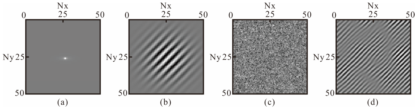
For better understanding, we present the convolution kernel $g_r$ and its corresponding noise field in Figure 1a,b.

Structured coherent artifacts generally exhibit directional continuity and spatial correlation, which cannot be described well by an independent random-noise model. Therefore, we make the assumption that coherent noise can be approximated through a linear noise model. Based on this, we have modified the convolutional kernel equation of the noise model, as shown in Equation (20). The modified convolution kernel and corresponding noise field are shown in Figure 1c,d.

$${\mathbf{g}}_c\left(x^{\left(1\right)},x^{\left(2\right)}\right)=\cos \left(k{x}^{\left(1\right)}+x^{\left(2\right)}\right)G_{10}\left(x^{\left(1\right)},x^{\left(2\right)}\right),$$

(20)

where $x^{\left(1\right)}$ and $x^{\left(2\right)}$ correspond to the horizontal and vertical grid indices, respectively, $G_{10}$ is a Gaussian (σ = 10) centered at the origin, and $k$ is a directional scaling factor applied to the horizontal grid index. By changing the relative contribution of the two spatial coordinates, $k$ controls the inclination angle of the coherent noise kernel and therefore determines the directional characteristics of the generated artifacts.

Equation (20) enables us to construct a linear noise convolution kernel that models noise characteristics of nonphysical events. When comparing the conventional independent noise model (Figure 1b) with our noise model (Figure 1d), the consistency of the estimated noise is clearly visible. Then, substituting Equation (21) into Equation (19), we can obtain the PSD equation of structured coherent artifact:

$${\mathit{\Psi }}_c=\left|\mathit{X}\right|{\left|F\left[{\mathit{g}}_c\right]\right|}^2.$$

(21)

Then, we can utilize the determined PSD of coherent noise to calculate the noise variance. The initial equation for the coherent noise variance, before any approximation, is accessible from Equation (12) and shown in Equation (22), which allows for subsequent derivations:

$$v_{i,j}^{x_1,\cdots ,x_M}=\mathit{var}\left\{{\sum }_{t=1}^M\left(b_j^1\right(t)s_i^{x_t}\right)\}.$$

(22)

Undergoing 2D variation, the spectral coefficient $s_i^{x_t}$ is written as follows:

$$s_i^{x_t}=⟨{\mathit{z}}_{x_t},b_i^2⟩=(\mathit{z}\ast {\stackrel{⃡}{b}}_i^2)(x_t),$$

(23)

where $\leftrightarrow$ is reflection about the origin, and by substituting Equation (23) into Equation (22), it can be obtained:

$$v_{i,j}^{x_1,\cdots ,x_M}=\mathit{var}\{{\sum }_{t=1}^M(b_j^1(t)s_i^{x_t}\}=\mathit{var}\{(\stackrel{⃡}{\mathit{z}}\ast b_i^2\ast {\tilde{b}}_j^1)\left(0\right)\}$$

(24)

Since $v_{i,j}^{x_1,\cdots ,x_M}$ is the noise variance, it has $\overleftrightarrow{z}=\overleftrightarrow{\eta }$. In addition, $\eta =\varphi \ast g$, and it can be shown that $\mathit{var}\{\left(\stackrel{⃡}{\mathit{z}}\ast b_i^2\ast {\tilde{b}}_j^1\right)\left(0\right)\}=\mathit{var}\left\{\left(\varphi \ast \stackrel{⃡}{\mathit{g}}\ast b_i^2\ast {\tilde{b}}_j^1\right)\left(0\right)\right\}$. Therefore, through Equation (24), we can define $v_{i,j}^{x_1,\cdots ,x_M}={‖\stackrel{⃡}{\mathit{g}}\ast b_i^2\ast {\tilde{b}}_j^1‖}_2^2$, where ${\tilde{b}}_j^1$ is an array with the same dimensions as $\mathit{z}$.

Then, by substituting Equation (21), we can obtain the noise variance equation of coherent noise as follows:

$$v_{i,j}^{x_1,\cdots ,x_M}={‖{\stackrel{⃡}{\mathit{g}}}_{\mathit{c}}\ast b_i^2\ast {\tilde{b}}_j^1‖}_2^2={‖{\left|\mathit{X}\right|}^{-2}{\mathit{\Psi }}_c{\left|F\left[b_i^2\right]\right|}^2{\left|F[{\tilde{b}}_j^1]\right|}^2‖}_1.$$

(25)

Note that this variance estimator provides a noise-aware weighting term for the subsequent collaborative filtering process. Unlike the constant variance assumption used for independent random noise, the estimated variance varies with the directional coherent-noise PSD and therefore reflects the spatial and directional distribution of structured artifacts. This allows the method to apply stronger suppression to artifact-dominated coefficients while reducing unnecessary attenuation of useful structures.

2.3.2. Advanced Block Matching Based on Coherent Noise Variance

Following the development of a coherent noise variance estimation method, Section 2.3.2 focuses on refining the block matching process within the collaborative filtering framework. By incorporating the newly established noise variance model, we aim to significantly enhance the accuracy of block matching.

As mentioned in Section 2.2.1, the block matching process [47] is to make the equation $J={‖E\left\{z_{x_R}-z_{x_j}\right\}‖}_2^2$ small. Based on this, we can derive the difference between different data blocks, which can be shown in Equation (26):

$${‖{\mathit{z}}_{x_R}-{\mathit{z}}_{x_j}‖}_2^2=2{\sum }_{i=1}^N{⟨\left[s_i^{x_R},s_i^{x_j}\right],b_2^1⟩}^2=2{\sum }_{i=1}^N{\left(s_{i,2}^{x_R,x_j}\right)}^2,$$

(26)

where $b_2^1=1/\sqrt{2}\left[1,-1\right]$, $s_i^{x_R}$ and $s_i^{x_j}$ represent the spectra coefficients through 2D transform, and ${\left(s_{i,2}^{x_R,x_j}\right)}^2$ arises from the squares of independent normal random variables with non-zero means. This statistical property qualifies it as a non-central chi-square random variable possessing one degree of freedom. The expectation of this specific distribution is given by the following expression:

$$E\left\{{\left(s_{i,2}^{x_R,x_j}\right)}^2\right\}=v_{i,2}^{x_R,x_j}+E^2\left\{s_{i,2}^{x_R,x_j}\right\}$$

(27)

Therefore, we can rewrite $J={‖E\left\{z_{x_R}-z_{x_j}\right\}‖}_2^2$ as follows:

$$J={‖E\left\{{\mathit{z}}_{x_R}-{\mathit{z}}_{x_j}\right\}‖}_2^2=2{\sum }_{i=1}^N{E}^2\left\{s_{i,2}^{x_R,x_j}\right\}$$

(28)

Then, Equation (26) can be rewritten through utilizing Equations (27) and (28):

$$E\left\{{‖{\mathit{z}}_{x_R}-{\mathit{z}}_{x_j}‖}_2^2\right\}={‖E\left\{{\mathit{z}}_{x_R}-{\mathit{z}}_{x_j}\right\}‖}_2^2+2{\sum }_{i=1}^N{v}_{i,2}^{x_R,x_j},$$

(29)

where the estimate of $J$ can be obtained, and the equation is shown as follows:

$$J={‖E\left\{{\mathit{z}}_{x_R}-{\mathit{z}}_{x_j}\right\}‖}_2^2=E\left\{{‖{\mathit{z}}_{x_R}-{\mathit{z}}_{x_j}‖}_2^2\right\}-2{\sum }_{i=1}^N{v}_{i,2}^{x_R,x_j}.$$

(30)

Finally, we can obtain the ordering equation through Equation (30):

$$L_{x_R}(x_j)={‖{\mathit{z}}_{x_R}-{\mathit{z}}_{x_R}‖}_2^2-2{\sum }_{i=1}^N{v}_{i,2}^{x_R,x_j},$$

(31)

2.3.3. Paired-Observation Similarity Strategy

With the block matching process optimized for handling coherent noise, Section 2.3.3 focuses on the subsequent step in our advanced collaborative filtering framework: enhancing the shrinkage and aggregation procedures. Traditionally, the BM3D framework calculates the similarity between original data and initial denoising results primarily during the ‘hard thresholding’ and ‘Wiener filtering’ steps of the shrinkage process. This standard approach falls short in handling the complex noise structures.

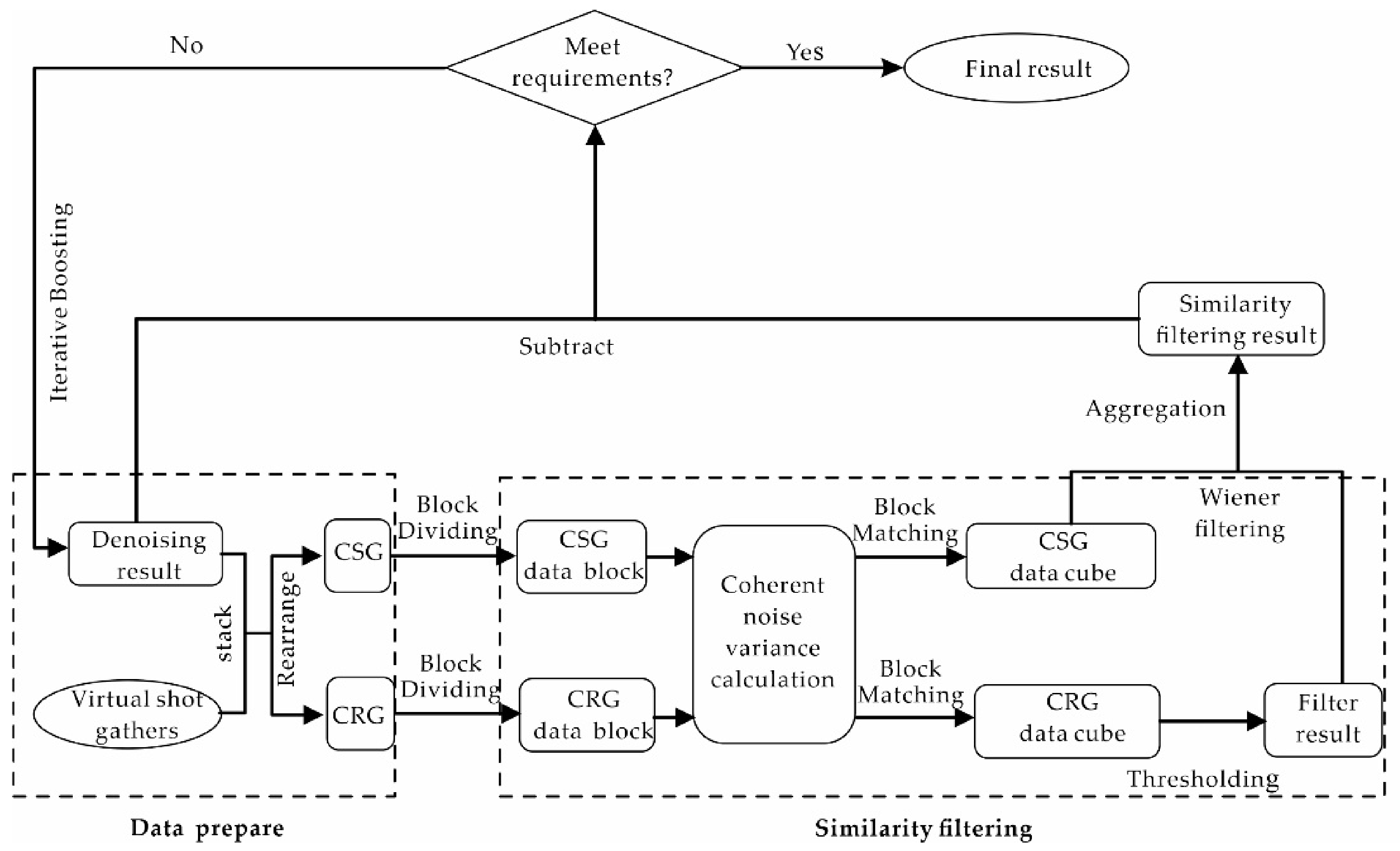
To bridge this gap, we introduce a paired-observation similarity strategy into the collaborative filtering framework (Figure 2). Instead of relying only on similarity calculations within a single noisy image, the proposed method exploits the structural similarity between two related observations of the same target. For virtual shot gathers, this paired-observation relationship is realized by the reciprocal consistency between CSGs and CRGs. This adjustment preserves the denoising principle of collaborative filtering while extending it to redundantly observed data. Furthermore, in order to balance computational efficiency and accuracy, we incorporated the SOS (strengthen−operate−subtract) boosting algorithm [48] into the overall process, which is an iterative process divided into three steps. The calculation equation is shown in Equation (32):

• Add the denoising result from the previous iteration to the input noise-contaminated data to strengthen the signal.
• Perform denoising on the signal strengthened data from the above step.
• The denoised image from the prior iteration is subtracted from the outcome of the signal-enhanced and reconstructed data:

$${\mathit{Y}}^{k+1}=C\left(\mathit{D}+{\mathit{Y}}^k\right)-{\mathit{Y}}^k,$$

(32)

where $C$ is the collaborative filtering framework proposed in this method, and $Y^0=0$.

To provide a clearer description of the implementation procedure, the complete computational workflow of the proposed consistency-guided collaborative filtering framework is summarized in Algorithm 1. The algorithm integrates coherent-noise characterization, consistency-guided block matching, collaborative shrinkage and aggregation, and SOS boosting into a unified iterative procedure. The coherent-noise PSD and variance are first estimated to characterize the directional and spatial correlation of the structured artifacts. These noise statistics, together with the paired-observation consistency, are subsequently incorporated into block matching and collaborative filtering to improve the discrimination between useful structures and inconsistent artifact components.

Algorithm 1. Pseudocode of the Proposed Consistency-Guided Collaborative Filtering Framework

Input: Noisy observation D; paired observation P; patch size b; search window size w;     number of matched blocks N; kernel parameter k; number of SOS iterations T; Initialization: iteration index t = 1; the denoised estimate $Y^0=0$. Construct the coherent-noise convolution kernel $g_k$ according to Equation (20). Estimate the coherent-noise PSD ${\mathsf{\Psi }}_c$ using Equations (16)–(21). Compute the coherent-noise variance map $v_{i,j}$ using Equations (22)–(25). While t ≤ T do:   Strengthen the signal according to the SOS strategy in Equation (32).     for each reference block Br in the strengthened observation do        Extract the corresponding paired block from P.        Compute the consistency-guided block similarity using the paired observation and the coherent-noise variance (Equations (26)–(31)).        Search the local window and select the N most similar blocks.        Stack the matched blocks into a 3D group.        Apply 2D intra-block transform and 1D inter-block transform.        Perform shrinkage guided by paired-observation consistency and coherent-noise PSD.        Apply the inverse 3D transform to obtain block estimates.        Aggregate all block estimates with weights to reconstruct the filtered observation.     end for   Update the denoised estimate according to Equation (32).   Set t = t + 1. end while Output: The final denoised result $Y^T$.

3. Results

3.1. Hyperspectral Remote-Sensing Image Example

A hyperspectral remote-sensing image was first used to evaluate the proposed framework under a controlled structured-artifact setting. Hyperspectral images provide redundant spatial–spectral observations, while stripe-like artifacts caused by detector nonuniformity and calibration residuals generally exhibit strong spatial correlation and directional continuity. One spectral band was selected as the target image, and the average of its neighboring bands was used as the paired observation because adjacent hyperspectral bands generally share similar spatial structures. Stripe-like structured coherent artifacts were then simulated and added to the target band. To provide a broader comparison, conventional BM3D, low-rank spatial-spectral restoration, and self-supervised learning-based restoration were selected as representative baselines. These methods correspond to classical collaborative filtering, modern model-driven reconstruction, and recent learning-based restoration, respectively, allowing the proposed framework to be evaluated against different types of hyperspectral artifact-removal strategies.

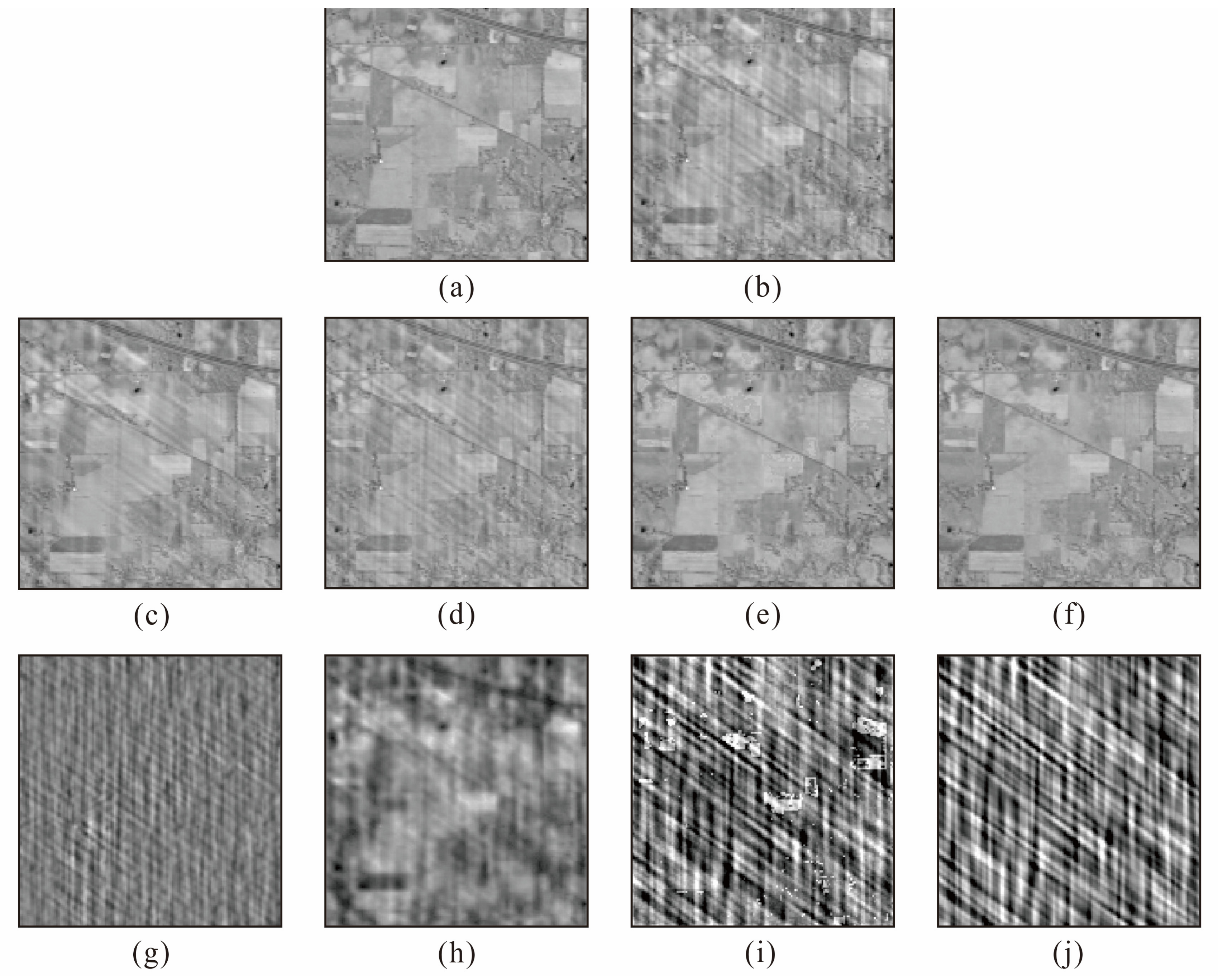
Figure 3 compares the restoration performance of different representative methods for suppressing stripe-like structured coherent artifacts. The contaminated image (Figure 3b) exhibits pronounced directional stripe patterns that obscure spatial textures and local structural details relative to the clean reference (Figure 3a). Conventional BM3D provides a reasonable restoration result and suppresses part of the stripe contamination (Figure 3c); however, inclined stripe residuals are still visible, and its removed component (Figure 3g) also indicates local over-denoising, suggesting that BM3D cannot fully distinguish directional structured artifacts from useful image details. The low-rank spatial–spectral restoration method further attenuates stripe-like artifacts by exploiting low-rank and spatial–spectral redundancy (Figure 3d), but the restored image appears over-smoothed, and some local textures and boundaries become less distinct. This indicates that when structured noise and useful image information are strongly coupled, the low-rank constraint has difficulty selectively suppressing the noise without affecting fine spatial details. The self-supervised learning-based restoration method achieves visually strong denoising performance and produces a cleaner restored image (Figure 3e); however, its removed component (Figure 3i) contains noticeable fine-scale scene-related structures, suggesting that part of the useful image information is also attenuated during denoising. In contrast, the proposed framework produces a result visually closer to the clean reference (Figure 3f), with substantially reduced stripe contamination while retaining clearer boundaries, spatial textures, and local structural details. Its removed component (Figure 3j) is dominated by directional stripe-like patterns and contains comparatively less obvious leakage of underlying spatial structures. These results demonstrate that the proposed framework achieves a more favorable balance between structured-artifact suppression and useful-information preservation, which is consistent with the additional discrimination provided by paired-observation consistency.

To quantitatively evaluate the restoration performance, four metrics, including PSNR, SSIM, RMSE, and MAE, were calculated for the contaminated image and the results obtained by different methods. As shown in

Table 1. Quantitative comparison between different methods for hyperspectral image restoration.

Method	PSNR	SSIM	RMSE	MAE
Contaminated	29.81	0.8224	0.0323	0.0258
BM3D	31.36	0.8731	0.0270	0.0214
LR	30.77	0.8501	0.0289	0.0231
ML	32.068	0.92455	0.0236	0.0189
Proposed	33.99	0.9334	0.0200	0.0157

, the proposed framework achieves the best quantitative performance among all compared methods, with the highest PSNR and SSIM values and the lowest RMSE and MAE values. Compared with conventional BM3D, the PSNR increases from 31.36 dB to 33.99 dB, and the SSIM increases from 0.8731 to 0.9334, indicating improved restoration accuracy and structural preservation. Compared with the LR (low-rank spatial–spectral method) and ML (self-supervised learning-based method), the proposed framework also provides better quantitative results. These improvements are consistent with the visual comparison in Figure 3, demonstrating that paired-observation consistency and coherent-noise-aware shrinkage are effective for suppressing stripe-like structured artifacts while preserving useful spatial information.

3.2. Synthetic Virtual Shot-Gather Example

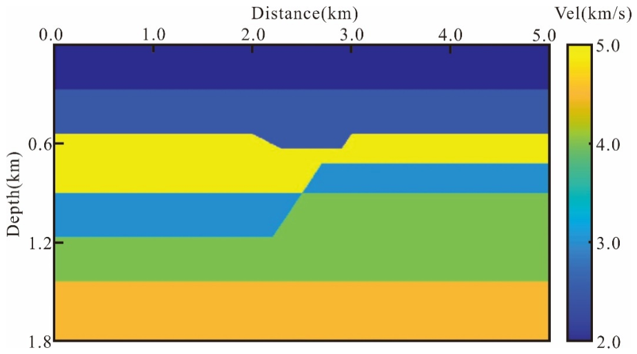
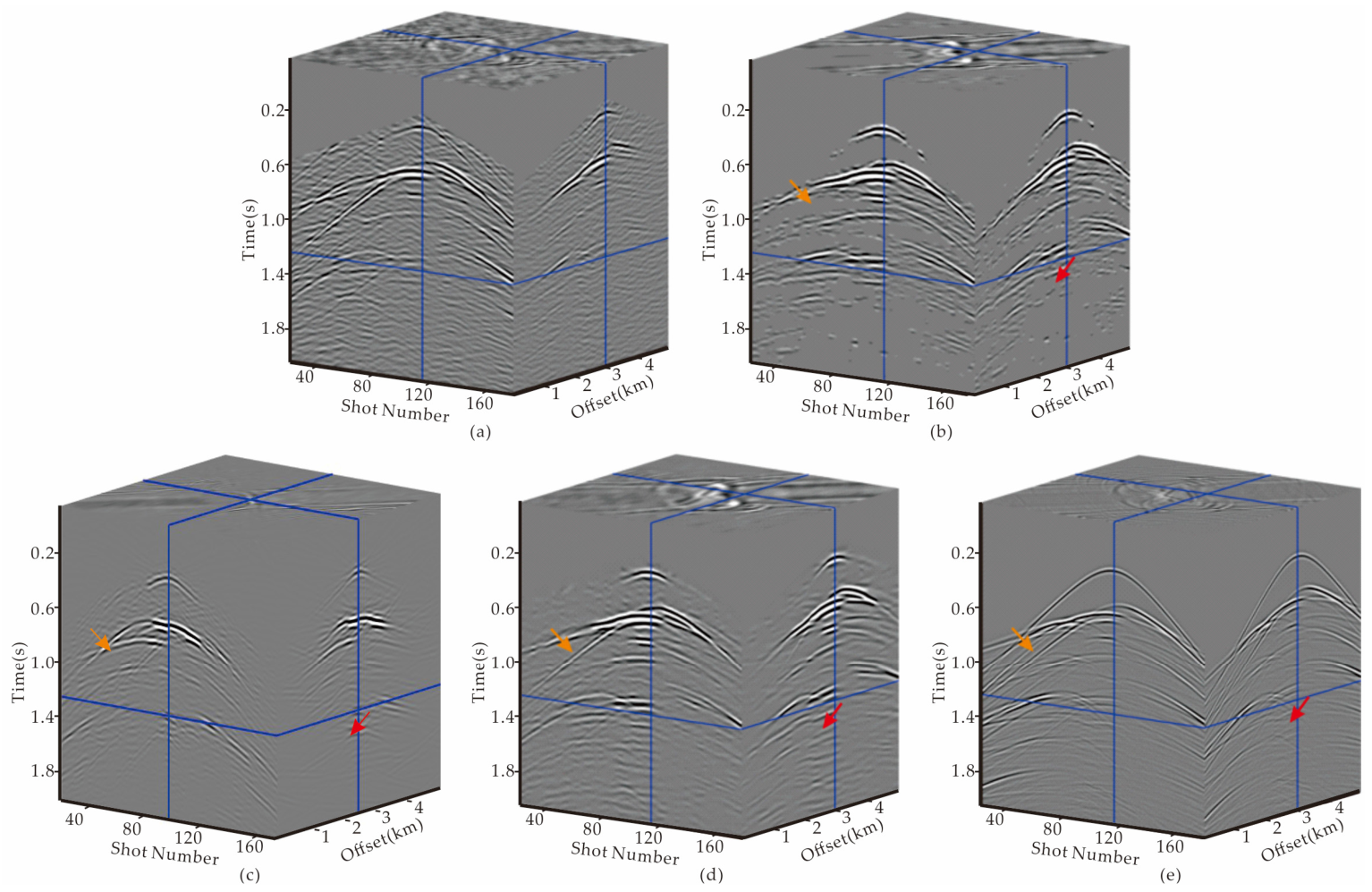
A synthetic virtual shot-gather test was then conducted to evaluate the proposed framework in a passive geophysical sensing scenario. The velocity model used in this study (Figure 4) contained several complex geological structures, including a high-velocity layer, faults, and sunken strata. These structures generated complex wavefields with attenuated events and multiple reflections, which made the suppression of nonphysical coherent events more challenging. Virtual shot gathers were constructed by conventional cross-correlation, including 251 shot positions, 251 receivers, and 1500 samples with a temporal interval of 2 ms. To evaluate the performance of the proposed framework, the synthetic data were analyzed from three perspectives: 3D data volumes, F-K spectra, and migration imaging results. The similarity-based filtering method and curvelet-based filtering method were used as representative comparison methods, and noise-free active-source seismic data were provided as a reference.

Figure 5 compares the 3D wavefield volumes obtained from the original virtual shot gathers (Figure 5a), the similarity-based filtering method (Figure 5b), the curvelet-based filtering method (Figure 5c), the proposed framework (Figure 5d), and the active-source reference (Figure 5e). The three axes represent sampling time, shot number, and offset. The original virtual shot gathers contain numerous nonphysical coherent events that interfere with the continuity and identification of the useful reflections. Both conventional approaches attenuate part of these artifacts, but their limitations remain visible in representative regions marked by the orange and red arrows. The similarity-based result still contains residual coherent events and local discontinuities of the reflection events (Figure 5b). Curvelet-based filtering further suppresses part of the directional coherent energy (Figure 5c), but some residual artifacts remain and local reflection characteristics are altered. In comparison, the proposed framework provides a cleaner wavefield while retaining better continuity of the major reflection events (Figure 5d). In the regions highlighted by the arrows, its event morphology shows closer agreement with the active-source reference (Figure 5e), indicating an improved balance between coherent-artifact attenuation and useful-signal preservation.

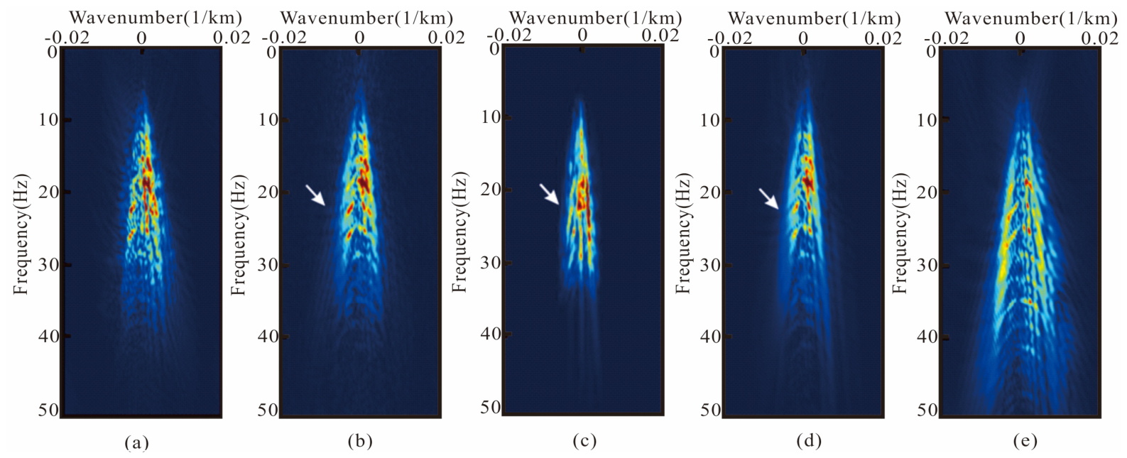
To further evaluate the performance of the different methods from the frequency–wavenumber perspective, the F-K spectra corresponding to the five datasets in Figure 5 are compared in Figure 6. Figure 6e shows the spectrum of the active-source reference. Because the virtual shot gathers lack far-offset observations, the corresponding far-offset traces of the active-source data were removed before calculating its F-K spectrum to ensure a more consistent comparison. Compared with the original virtual shot gathers (Figure 6a), all three processing methods attenuate part of the artifact-related spectral energy and improve the concentration of the dominant spectral components. However, clear differences remain among the processed results. The similarity-based result (Figure 6b) still exhibits spectral discontinuities and weakened energy around the region indicated by the white arrow. Curvelet-based filtering (Figure 6c) effectively suppresses a considerable portion of the coherent spectral components, but the resulting spectrum becomes relatively concentrated and some useful spectral energy is weakened. In comparison, the proposed framework (Figure 6d) suppresses the artifact-related energy while maintaining better continuity and distribution of the dominant spectral components. Its spectral characteristics show closer agreement with those of the active-source reference (Figure 6e), particularly in the frequency range highlighted by the arrows. These results further demonstrate that the proposed framework achieves a better balance between coherent-artifact attenuation and preservation of useful wavefield information.

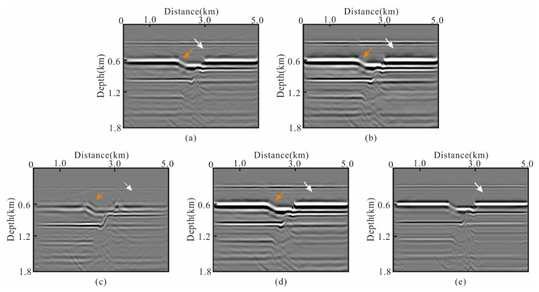
Figure 7 further compares the migration imaging results obtained from the five datasets, providing an imaging-domain assessment of the different artifact-suppression strategies. The migration image obtained from the original virtual shot gathers (Figure 7a) contains noticeable false reflections and locally distorted structures caused by the nonphysical coherent events. After similarity-based filtering (Figure 7b), part of these imaging artifacts is attenuated; however, residual false reflections remain around the region indicated by the white arrow, while the structural continuity near the inclined and depressed strata highlighted by the orange arrow is not fully recovered. Curvelet-based filtering (Figure 7c) suppresses part of the coherent energy, but the resulting image contains stronger residual and redistributed energy at greater depths, together with reduced continuity of several reflection interfaces. In comparison, the proposed framework (Figure 7d) more effectively suppresses the artifact-related reflections while preserving the geometry and continuity of the principal subsurface structures. In particular, the shallow reflection indicated by the white arrow is better recovered, and the inclined structure around the orange arrow shows a clearer morphology that is more consistent with the active-source reference (Figure 7e). These imaging results confirm that the proposed framework provides a more favorable balance between suppression of nonphysical coherent events and preservation of geologically meaningful reflections.

3.3. Field Virtual Shot-Gather Example

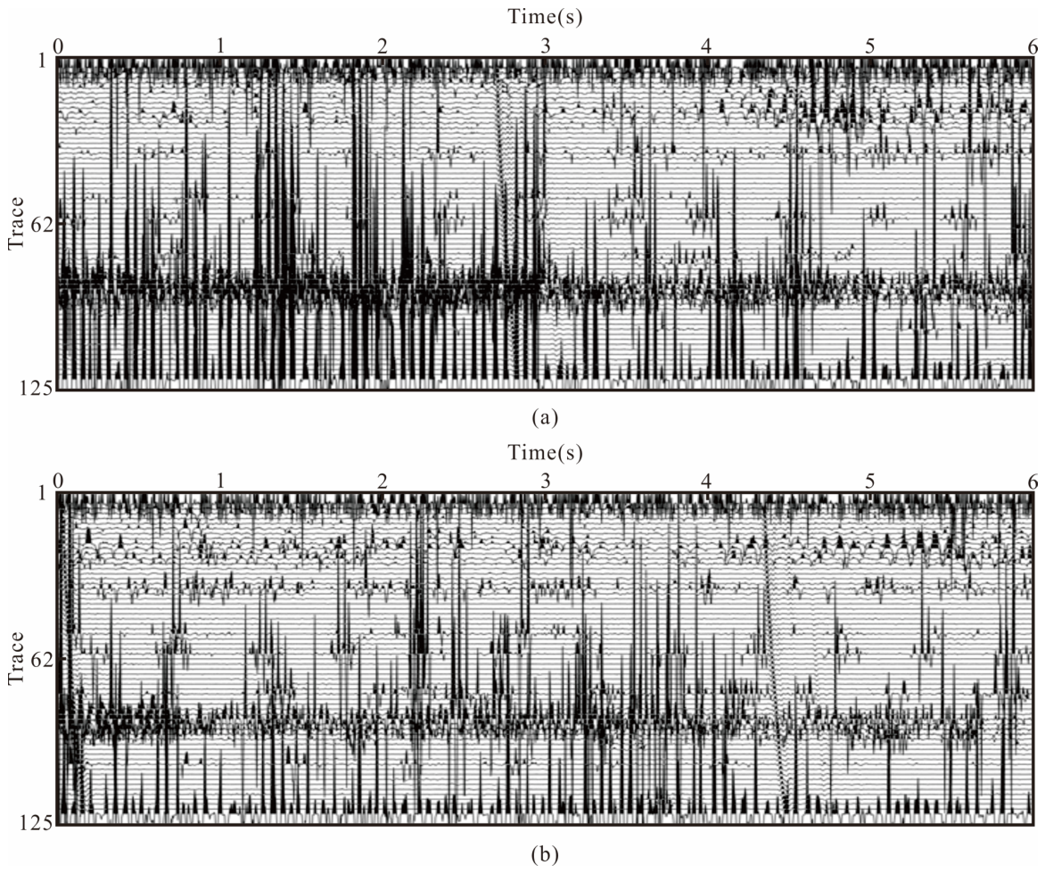
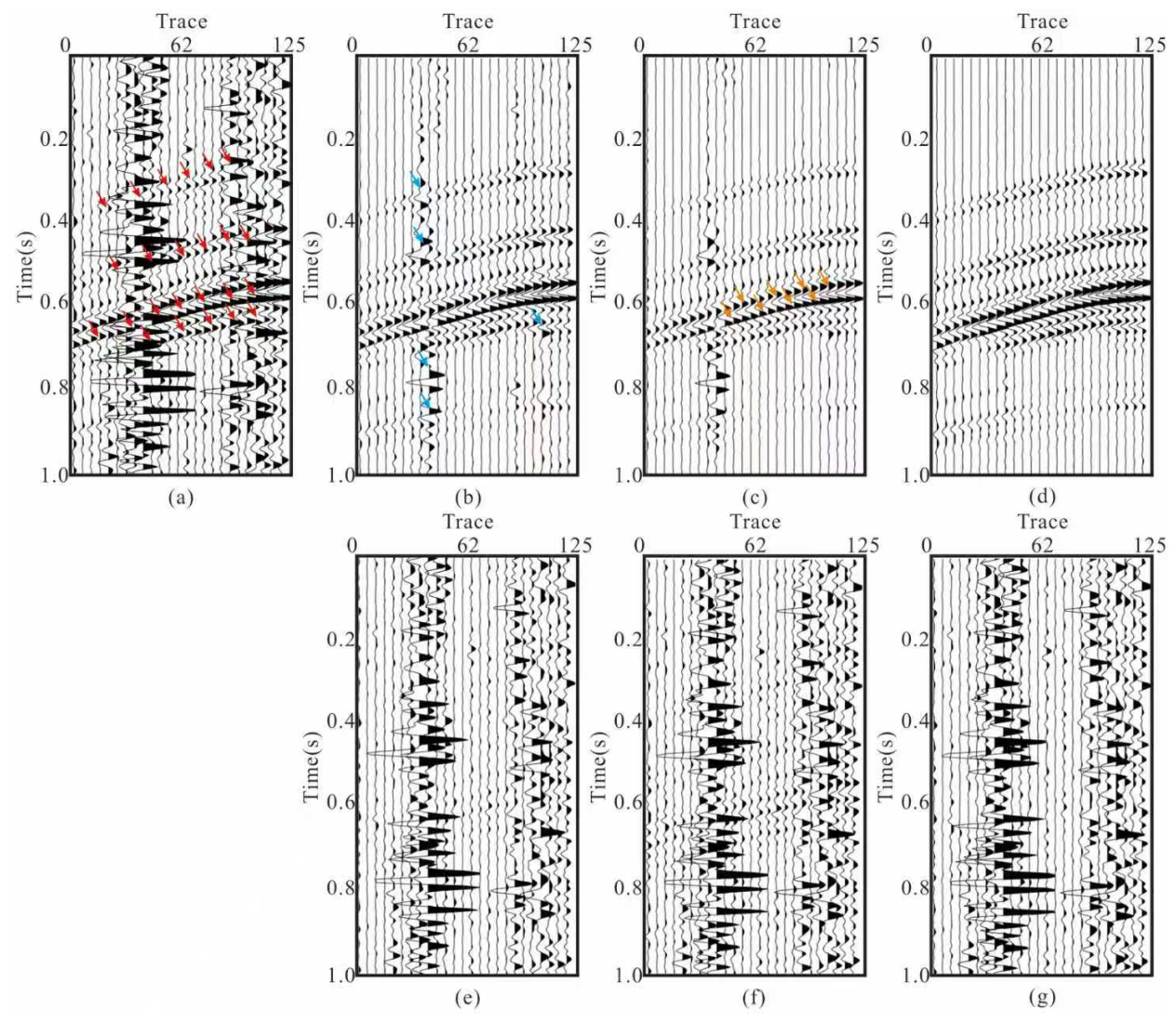
Furthermore, we applied the proposed framework to a field passive seismic data to test its stability in facing complex wavefield. In Figure 8, we show the utilized field data, which is a borehole microseismic dataset with 125 receivers. The total sampling duration was 10 min with a sampling interval (dt) of 0.002 s. For display purposes, we randomly selected two windowed data, each 6 s in duration. From Figure 8, it can be observed that the field seismic data contain not only seismic signals but also a substantial amount of noise with strong energy, which poses a significant challenge for the proposed framework.

We applied the complete data preprocessing workflow for passive source data (including bandpass filtering, Normal Moveout (NMO), outlier removal, median filtering, inverse NMO, and amplitude equalization) to the original data before using seismic interferometry to generate a virtual shot gather. Then, the generated virtual shot gather, as shown in Figure 9a, exhibits substantial high-energy noise that severely obscures useful events. In Figure 9a, we marked some of the useful events with red arrows, showing that these signals are almost masked by coherent noise. Figure 9 shows that all three methods attenuate part of the coherent interference and improve the visibility of the main reflection events relative to the original gather (Figure 9a). However, clear differences remain among the processed results. The similarity-based denoising result (Figure 9b) still contains noticeable residual strong coherent noise, as indicated by the blue arrows, showing that the method does not fully suppress the dominant interference. Curvelet-based filtering (Figure 9c) provides stronger attenuation of the coherent noise, but the events indicated by the orange arrows become weakened or partially distorted, suggesting that useful reflection information is also affected during the filtering process. In comparison, the proposed framework (Figure 9d) produces a cleaner virtual shot gather while maintaining clearer and more continuous event structures. The removed components shown in Figure 9e–g provide additional evidence for the different filtering behaviors. These results indicate that the proposed framework achieves a more favorable balance between suppressing coherent artifacts and preserving useful wavefield information in field data.

4. Discussion

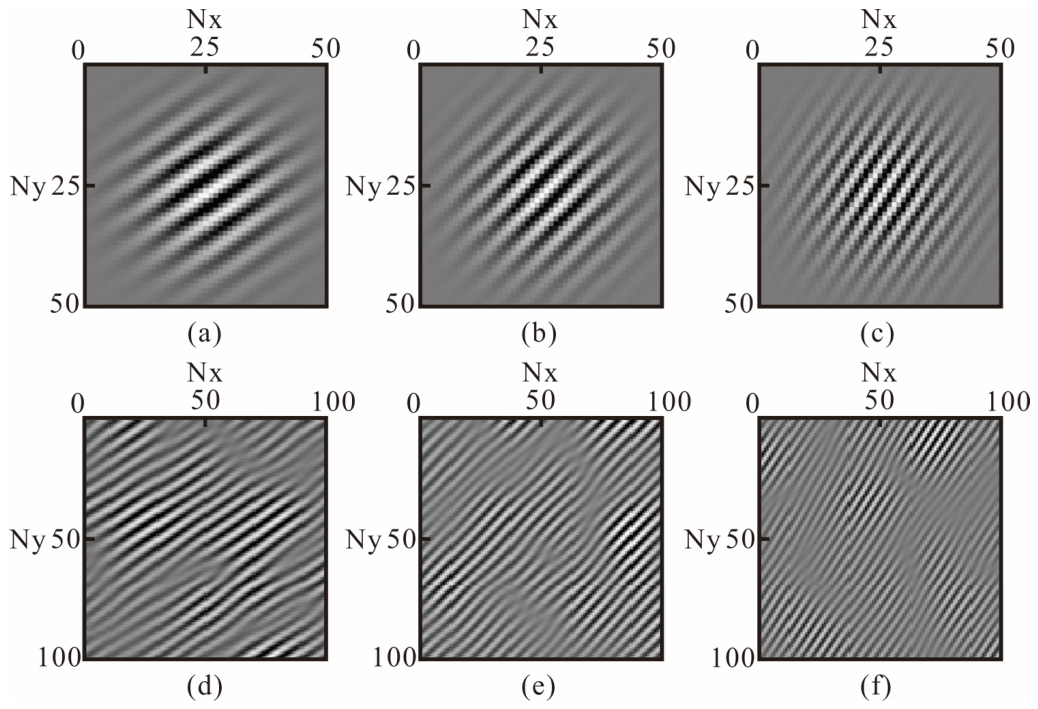
For the proposed framework, an accurate noise model is a crucial factor, as it directly affects the performance of the collaborative filtering process. In the PSD-based formulation, the convolution kernel is used to describe the directional and spatial correlation of structured coherent artifacts. For virtual shot gathers, the main type of noise is nonphysical noise with relatively high apparent velocities, which typically manifests in images as features with steep angles. To address this characteristic, we can adjust the parameter k in Equation (20) to modify the noise model to better fit the actual conditions. In Figure 10, we demonstrate the impact of different k values on the constructed convolution kernels and the corresponding noise models. Figure 10a,d correspond to a k value of 2/3, Figure 10b,e correspond to a k value of 1, and Figure 10c,f correspond to a k value of 3/2. It can be observed that as the k value increases, the inclination angle of both the convolution kernel and noise model also increases. Therefore, we recommended to first analyze the spatial and temporal distribution of noise events in the data which need to be processed to calculate their inclination angles, and then select a suitable k value based on these angles. It should be noted that k is not treated as an arbitrary empirical parameter in the proposed framework. Instead, it is determined according to the dominant apparent inclination of the structured coherent artifacts. In practical applications, the inclination of the dominant noise events can be estimated from the data or their spectral characteristics, and the corresponding k value is then used to construct the coherent-noise convolution kernel to avoid errors caused by inappropriate parameter selection. Other collaborative-filtering parameters, including the block size, search-window size, shrinkage threshold, and SOS boosting iteration number, were fixed across the compared methods and experiments to ensure fair comparison. Therefore, the parameter selection mainly concerns the directional parameter k, which is determined from the dominant artifact inclination rather than by exhaustive trial-and-error optimization.

Computational efficiency is also a key factor. The proposed framework is developed based on the conventional BM3D collaborative filtering framework, where block matching, transform-domain shrinkage, and aggregation are retained as the fundamental procedures. Therefore, the computational complexity of the proposed method mainly consists of the original BM3D operations and the additional computational costs introduced by paired-observation consistency analysis, coherent noise PSD estimation, and SOS boosting-based iterative refinement. For an input dataset with N samples, the block matching procedure in BM3D dominates the computational cost and can be approximately expressed as O(NK), where K denotes the number of candidate patches searched within the predefined neighborhood. The transform-domain shrinkage and aggregation procedures mainly involve forward/inverse transformations and weighted reconstruction, with an approximate complexity of O (N log N). Compared with conventional BM3D, the proposed method introduces additional similarity estimation between paired observations and PSD calculation to characterize the spatial correlation and directional distribution of structured coherent artifacts. Moreover, the SOS boosting strategy repeatedly updates the denoised result by performing multiple refinement iterations, which further increases the computational cost proportional to the number of boosting iterations.

To further evaluate the computational efficiency, the runtime of different methods was compared under the same experimental environment. As shown in

Table 2. Runtime comparison of different methods.

Method	BM3D	LR	ML	Proposed
Runtime (s)	0.99	1.24	34.47	3.75

, the proposed method requires a runtime of approximately 3.75 s, which is higher than conventional BM3D (approximately 0.99 s). This increased computational cost mainly results from three additional procedures: paired-observation consistency estimation, coherent noise PSD modeling, and SOS boosting-based iterative refinement. In particular, the SOS boosting strategy requires multiple executions of the denoising process to progressively improve artifact suppression performance, leading to additional computational overhead. However, compared with the ML (approximately 34.47 s), the proposed framework achieves substantially higher computational efficiency because it does not require feature training or model inference. These results indicate that the proposed method achieves a favorable balance between computational cost and denoising performance, providing improved suppression of structured coherent artifacts while maintaining acceptable processing efficiency.

The key element of the proposed framework is the construction of paired observations. The framework assumes that useful structures are relatively stable between paired observations, while structured coherent artifacts exhibit stronger inconsistencies, directionality, or observational dependencies. In hyperspectral remote-sensing images, adjacent spectral bands can provide paired observations because they typically possess similar spatial textures and land cover structures. This also implies that directional modeling is important for stripe artifacts in hyperspectral remote-sensing images, even though their physical origins differ from the nonphysical events in virtual shot gathers. Therefore, the proposed framework is particularly suitable for redundantly observed sensing data, where useful information is repeatable or structurally consistent across paired observations, whereas artifacts are directionally coherent but less consistent between observations. Beyond the examples tested in this study, the same idea may be extended to multi-temporal remote sensing images, multi-view or multi-angle imaging data, repeated geophysical observations, and other sensing scenarios with meaningful observational redundancy. Future work will focus on adaptive paired-observation construction to further improve its applicability to broader sensing scenarios.

5. Conclusions

This study proposed a consistency-guided collaborative filtering framework for suppressing structured coherent artifacts in redundantly observed data. By combining paired-observation consistency with coherent noise modeling, the proposed framework can attenuate inconsistent artifact components while preserving stable useful structures. Experiments on hyperspectral remote-sensing images show that the method effectively suppresses stripe-like artifacts and better preserves spatial textures and edge information. Synthetic and field virtual shot-gather tests further demonstrate its ability to suppress nonphysical coherent events while maintaining reflection continuity and amplitude fidelity. These results indicate that the proposed framework provides an effective and flexible strategy for improving imaging reliability in remote-sensing and geophysical sensing data affected by structured coherent artifacts.

References

1. Wapenaar, K.; Draganov, D.; Snieder, R.; Campman, X.; Verdel, A. Tutorial on seismic interferometry: Part 1—Basic principles and applications. Geophysics 2010, 75, 75A195–75A209. [Google Scholar] [CrossRef] [Scilit]
2. Zhang, H.; He, W.; Zhang, L.; Shen, H.; Yuan, Q. Hyperspectral image restoration using low-rank matrix recovery. IEEE Trans. Geosci. Remote Sens. 2014, 52, 4729–4743. [Google Scholar] [CrossRef] [Scilit]
3. Zhuang, L.; Bioucas-Dias, J.M. Fast hyperspectral image denoising and inpainting based on low-rank and sparse representations. IEEE J. Sel. Top. Appl. Earth Obs. Remote Sens. 2018, 11, 730–742. [Google Scholar] [CrossRef] [Scilit]
4. Gómez-Chova, L.; Alonso, L.; Guanter, L.; Camps-Valls, G.; Calpe, J.; Moreno, J. Correction of systematic spatial noise in push-broom hyperspectral sensors: Application to CHRIS/PROBA images. Appl. Opt. 2008, 47, F46–F60. [Google Scholar] [CrossRef] [Scilit] [PubMed]
5. Adler-Golden, S.M.; Richtsmeier, S.C.; Conforti, P.F.; Bernstein, L.S. Spectral image destriping using a low-dimensional model. Proc. SPIE 2013, 8743, 87431Q. [Google Scholar] [CrossRef] [Scilit]
6. Beckel, R.A.; Juhlin, C. Impact of source and receiver distributions on imaging of dipping reflectors with passive reflection seismic interferometry. Geophys. J. Int. 2022, 230, 2098–2116. [Google Scholar] [CrossRef] [Scilit]
7. Chen, Y.; Huang, T.-Z.; Zhao, X.-L.; Deng, L.-J.; Huang, J. Stripe noise removal of remote sensing images by total variation regularization and group sparsity constraint. Remote Sens. 2017, 9, 559. [Google Scholar] [CrossRef] [Scilit]
8. Wang, Y.; Peng, J.; Zhao, Q.; Leung, Y.; Zhao, X.-L.; Meng, D. Hyperspectral Image Destriping and Denoising Using Stripe and Spectral Low-Rank Matrix Recovery and Global Spatial-Spectral Total Variation. Remote Sens. 2021, 13, 827. [Google Scholar] [CrossRef] [Scilit]
9. Zhang, Z.; Yang, F. Hyperspectral image denoising and destriping based on sparse representation, graph Laplacian regularization and stripe low-rank property. EURASIP J. Adv. Signal Process. 2022, 2022, 96. [Google Scholar] [CrossRef] [Scilit]
10. Peng, C.; Liu, Y.; Chen, Y.; Wu, X.; Cheng, A.; Kang, Z.; Chen, C.; Cheng, Q. Hyperspectral Image Denoising Using Nonconvex Local Low-Rank and Sparse Separation with Spatial–Spectral Total Variation Regularization. IEEE Trans. Geosci. Remote Sens. 2022, 60, 5538617. [Google Scholar] [CrossRef] [Scilit] [PubMed]
11. Lai, Q.; Fu, Y.; Xiang, W.; He, F.; Zhan, T. TRQ3DNet: A 3D Quasi-Recurrent and Transformer Based Network for Hyperspectral Image Denoising. Remote Sens. 2022, 14, 4598. [Google Scholar] [CrossRef] [Scilit]
12. Li, M.; Fu, Y.; Zhang, Y. Spatial-Spectral Transformer for Hyperspectral Image Denoising. Proc. AAAI Conf. Artif. Intell. 2023, 37, 1368–1376. [Google Scholar] [CrossRef] [Scilit]
13. Miao, Y.; Zhang, L.; Zhang, L.; Tao, D. DDS2M: Self-Supervised Denoising Diffusion Spatio-Spectral Model for Hyperspectral Image Restoration. In Proceedings of the IEEE/CVF International Conference on Computer Vision, Paris, France, 1–6 October 2023; pp. 12086–12096. [Google Scholar]
14. Artman, B. Imaging passive seismic data. Geophysics 2006, 71, SI177–SI187. [Google Scholar] [CrossRef] [Scilit]
15. Daneshvar, M.R.; Clay, C.S.; Savage, M.K. Passive seismic imaging using microearthquakes. Geophysics 1995, 60, 1178–1186. [Google Scholar] [CrossRef] [Scilit]
16. Snieder, R.; Miyazawa, M.; Slob, E.; Vasconcelos, I.; Wapenaar, K. A Comparison of Strategies for Seismic Interferometry. Surv. Geophys. 2009, 30, 503–523. [Google Scholar] [CrossRef] [Scilit]
17. Ramirez, A.C.; Weglein, A.B.; Otnes, E.; Hokstad, K. The role of the direct wave and Green’s theorem in seismic interferometry and spurious multiples. In SEG Technical Program Expanded Abstracts 2007; Society of Exploration Geophysicists: Houston, TX, USA, 2007; pp. 2471–2475. [Google Scholar]
18. Wang, Y.; Luo, Y.; Schuster, G.T. Interferometric interpolation of missing seismic data. Geophysics 2009, 74, SI37–SI45. [Google Scholar] [CrossRef] [Scilit]
19. Melo, G.; Malcolm, A.; Fehler, M. Comparison of microearthquake locations using seismic interferometry principles. In SEG Technical Program Expanded Abstracts 2012; Society of Exploration Geophysicists: Houston, TX, USA, 2012; pp. 1–5. [Google Scholar]
20. Gu, N.; Chamarczuk, M.; Gao, J.; Malinowski, M.; Zhang, H. Passive seismic structure imaging of a coal mine by ambient noise seismic interferometry on a dense array. Acta Geol. Sin.-Engl. Ed. 2021, 95, 37–39. [Google Scholar] [CrossRef] [Scilit]
21. Yu, J.; Kim, B.-Y.; Joo, Y. A processing for ocean-bottom multicomponent data with seismic interferometry: A case study of southern offshore in Korea. Explor. Geophys. 2023, 54, 533–543. [Google Scholar] [CrossRef] [Scilit]
22. Zhang, F.; Zhang, P.; Xu, Z.; Gong, X.; Han, L. Multisource Seismic Full Waveform Inversion of Metal Ore Bodies. Minerals 2022, 12, 4. [Google Scholar] [CrossRef] [Scilit]
23. Liu, Q.; Feng, X.; Liu, C.; Zhang, M.; Tian, Y.; Hou, H. Metallic mineral exploration by using ambient noise tomography in Ashele copper mine, Xinjiang, China. Geophysics 2022, 87, B221–B231. [Google Scholar] [CrossRef] [Scilit]
24. Brenguier, F.; Baue, P.; Ben-Zion, Y.; Vernon, F.; Johnson, C.W.; Mordret, A.; Countant, O.; Share, P.-E.; Beauce, E.; Hollis, D.; et al. Train Traffic as a Powerful Noise Source for Monitoring Active Faults with Seismic Interferometry. Geophys. Res. Lett. 2019, 46, 9529–9536. [Google Scholar] [CrossRef] [Scilit] [PubMed]
25. Mao, S.; Lecointre, A.; van der Hilst, R.D.; Campillo, M. Space-time monitoring of groundwater fluctuations with passive seismic interferometry. Nat. Commun. 2022, 13, 4643. [Google Scholar] [CrossRef] [Scilit] [PubMed]
26. Eisner, L.; Duncan, P.M.; Heigl, W.M. Uncertainties in passive seismic monitoring. Lead. Edge 2009, 28, 648–655. [Google Scholar] [CrossRef] [Scilit]
27. Delaney, E.; Ermert, L.; Sager, K.; Kritski, A.; Bussat, S.; Fichtner, A. Passive seismic monitoring with nonstationary noise sources. Geophysics 2017, 82, KS57–KS70. [Google Scholar] [CrossRef] [Scilit]
28. King, S.; Curtis, A. Suppressing nonphysical reflections in Green’s function estimates using source-receiver interferometry. Geophysics 2012, 77, Q15–Q25. [Google Scholar] [CrossRef] [Scilit]
29. Viens, L.; Van Houtte, C. Denoising ambient seismic field correlation functions with convolutional autoencoders. Geophys. J. Int. 2020, 220, 1521–1535. [Google Scholar] [CrossRef] [Scilit]
30. Othman, A.; Iqbal, N.; Hanafy, S.M.; Waheed, U.B. Automated Event Detection and Denoising Method for Passive Seismic Data Using Residual Deep Convolutional Neural Networks. IEEE Trans. Geosci. Remote Sens. 2022, 60, 2022. [Google Scholar] [CrossRef] [Scilit]
31. Zhang, P.; Han, L.-G.; Zhou, Y.; Xu, Z.; Ge, Q.-X. Passive-source multitaper-spectral method based low-frequency data reconstruction for active seismic sources. Appl. Geophys. 2015, 12, 585–597. [Google Scholar] [CrossRef] [Scilit]
32. Naghadeh, D.H.; Bean, C.J.; Brenguier, F.; Smith, P.J. Retrieving reflection arrivals from passive seismic data using Radon correlation. J. Geophys. Eng. 2021, 18, 177–191. [Google Scholar] [CrossRef] [Scilit]
33. Polychronopoulou, K.; Lois, A.; Draganov, D. Body-wave passive seismic interferometry revisited: Mining exploration using the body waves of local microearthquakes. Geophys. Prospect. 2020, 68, 232–253. [Google Scholar] [CrossRef] [Scilit]
34. Wapenaar, K.; van der Neut, J.; Ruigrok, E. Passive seismic interferometry by multidimensional deconvolution. Geophysics 2008, 73, A51–A56. [Google Scholar] [CrossRef] [Scilit]
35. Zhu, H.; Wang, D.-L.; Tsoflias, G.P. Seismic interferometry in parabolic Radon domain. J. Seism. Explor. 2015, 24, 37–50. [Google Scholar]
36. Cheng, H.; Wang, D.-L.; Feng, F.; Zhu, H. Estimating primaries from passive seismic data. Explor. Geophys. 2015, 46, 184–191. [Google Scholar] [CrossRef] [Scilit]
37. Fomel, S. Local seismic attributes. Geophysics 2007, 72, A29–A33. [Google Scholar] [CrossRef] [Scilit]
38. Hu, B.; Wang, D.; Wang, R. An Iterative Focal Denoising Strategy for Passive Seismic Data. Pure Appl. Geophys. 2020, 177, 4607–4622. [Google Scholar] [CrossRef] [Scilit]
39. Wang, T.; Wang, D.; Sun, J.; Hu, B. Passive seismic data primary estimation and noise removal via focal-denoising closed-loop surface-related multiple elimination based on 3D L1-norm sparse inversion. Geophys. Prospect. 2021, 69, 122–138. [Google Scholar] [CrossRef] [Scilit]
40. Hu, B.; Jia, Z.; Zhang, L. Coherent noise attenuation for passive seismic data based on iterative two-dimensional model shrinkage. Acta Geophys. 2021, 69, 773–782. [Google Scholar] [CrossRef] [Scilit]
41. Su, X.; Khoshgoftaar, T.M. A survey of collaborative filtering techniques. Adv. Artif. Intell. 2009, 2009, 421425. [Google Scholar] [CrossRef] [Scilit]
42. Ghazanfar, M.; Prugel-Bennett, A. An improved switching hybrid recommender system using naive bayes classifier and collaborative filtering. In Proceedings of the 2010 IAENG International Conference on Data Mining and Applications, Hong Kong, China, 17–19 March 2010. [Google Scholar]
43. Chierchia, G.; El Gheche, M.; Scarpa, G.; Verdoliva, L. Multitemporal SAR Image Despeckling Based on Block-Matching and Collaborative Filtering. IEEE Trans. Geosci. Remote Sens. 2017, 55, 5467–5480. [Google Scholar] [CrossRef] [Scilit]
44. Dabov, K.; Foi, A.; Katkovnik, V.; Egiazarian, K. Image denoising by sparse 3-D transform-domain collaborative filtering. IEEE Trans. Image Process. 2007, 16, 2080–2095. [Google Scholar] [CrossRef] [Scilit] [PubMed]
45. Dabov, K.; Foi, A.; Katkovnik, V.; Egiazarian, K. Image restoration by sparse 3D transform-domain collaborative filtering. Proc. SPIE 2008, 6812, 681207. [Google Scholar] [CrossRef] [Scilit]
46. Rubel, A.; Lukin, V.; Egiazarian, K. Block matching and 3D collaborative filtering adapted to additive spatially correlated noise. In Proceedings of the Ninth International Workshop on Video Processing and Quality Metrics for Consumer Electronics—VPQM 2015, Chandler, AZ, USA, 5–6 February 2015; p. 6. [Google Scholar]
47. Rubel, A.S.; Lukin, V.V.; Egiazarian, K.O. Metric performance in similar blocks search and their use in collaborative 3D filtering of grayscale images. Proc. SPIE 2014, 9019, 65–76. [Google Scholar] [CrossRef] [Scilit]
48. Zhang, C.; van der Baan, M. Multicomponent microseismic data denoising by 3D shearlet transform. Geophysics 2018, 83, A45–A51. [Google Scholar] [CrossRef] [Scilit]
Figure 1. Comparison of convolution kernels before and after modification and their corresponding generated noise fields: (a,b) original and modified kernels; (c,d) generated random and structured coherent noise fields.
Remotesensing 18 02780 g001
Figure 2. Workflow of the consistency-guided collaborative filtering framework.
Remotesensing 18 02780 g002
Figure 3. Comparison of different methods for suppressing stripe-like structured coherent artifacts in a hyperspectral remote-sensing image: (a) clean band image; (b) contaminated image; (c) BM3D result; (d) SSLR-SSTV-inspired result; (e) self-supervised machine-learning result; (f) proposed result; (gj) their corresponding removed components.
Remotesensing 18 02780 g003
Figure 4. The velocity model for the synthetic example.
Remotesensing 18 02780 g004
Figure 5. Comparison of synthetic virtual shot-gather results obtained using different coherent-artifact suppression methods: (a) original virtual shot gathers; (b) similarity-based filtering result; (c) curvelet-based filtering result; (d) proposed framework; (e) active-source reference.
Remotesensing 18 02780 g005
Figure 6. F−K spectra of the synthetic virtual shot-gather results: (a) original virtual shot gathers; (b) similarity-based filtering result; (c) curvelet-based filtering result; (d) proposed framework; (e) active-source reference.
Remotesensing 18 02780 g006
Figure 7. Migration results: (a) original data; (b) similarity-based filtering result; (c) curvelet-based filtering result; (d) proposed result; (e) active-source reference.
Remotesensing 18 02780 g007
Figure 8. Original field passive seismic data: (a) raw data; (b) preprocessing result.
Remotesensing 18 02780 g008
Figure 9. Field virtual shot-gather comparison using different artifact-suppression methods: (a) original data; (b) similarity-based denoising result; (c) curvelet-based filtering result; (d) proposed result; (eg) their corresponding removed components.
Remotesensing 18 02780 g009
Figure 10. Display of convolutional kernel and noise model corresponding to different k value: convolution kernel with k = 2/3 (a), k = 1 (b), and k = 3/2 (c); noise model with k = 2/3 (d), k = 1 (e), and k = 3/2 (f).
Remotesensing 18 02780 g010