Article

Asynchronous Responses of Ecosystem Carbon Gain and Groundwater Storage Under Ecological Restoration in the Loess Plateau


1
School of Geomatics and Urban Spatial Informatics, Beijing University of Civil Engineering and Architecture, Beijing 102616, China
2
Center for Carbon Neutrality, Chinese Academy of Environmental Planning, Beijing 100043, China
3
State Key Laboratory of Remote Sensing and Digital Earth, Faculty of Geographical Science, Beijing Normal University, Beijing 100875, China
*
Author to whom correspondence should be addressed.
Remote Sens. 2026, 18(16), 2822; https://doi.org/10.3390/rs18162822
Submission received: 24 June 2026 / Revised: 14 August 2026 / Accepted: 16 August 2026 / Published: 20 August 2026

Highlights

What are the main findings?
  • During 2002–2023, GPP increased substantially faster than ET, with relative growth rates of 1.66% and 0.47%, respectively, resulting in a significant increase in WUE. XGBoost–SHAP analysis showed that LAI had the strongest model-based association with GPP and WUE, whereas ET was jointly associated with LAI, air temperature, and precipitation.
  • Middle- and deep-layer soil moisture showed an increasing tendency during 2016–2023, whereas regional groundwater storage declined markedly during 2002–2020 and showed only a short-term, nonsignificant increase during 2020–2023.
What are the implications of the main findings?
  • Ecological restoration was accompanied by increased ecosystem carbon gain and WUE without a proportional increase in annual ET, while improvements in surface carbon–water conditions did not translate into synchronous groundwater recovery.
  • Integrating multi-source remote sensing, land-surface assimilation, GRACE/GRACE-FO, and human water-use datasets provides useful evidence for optimizing ecological restoration and groundwater management.

Abstract

Since the implementation of the Grain-for-Green Program (GGP), vegetation across the Loess Plateau (LP) has substantially recovered. However, whether the associated increase in ecosystem carbon gain was accompanied by a proportional increase in water consumption and whether groundwater storage changed synchronously remain unclear. This study integrated multi-source remote sensing products, GLDAS-Noah land-surface assimilation data, GRACE/GRACE-FO satellite gravimetry, irrigation water-use data, provincial water-use statistics, and coal-resource information to examine long-term changes in gross primary productivity (GPP), evapotranspiration (ET), water-use efficiency (WUE), soil moisture (SM), and groundwater storage anomaly (GWSA) during 2002–2023. GPP increased significantly by 10.67 g C m−2 yr−1 ( p < 0.01 ), whereas ET increased more modestly by 1.97 mm yr−1 ( p < 0.05 ). The relative growth rate of GPP (1.66%) was approximately 3.5 times that of ET (0.47%), and WUE increased by 0.018 g C m−2 mm−1 yr−1 ( p < 0.01 ). In the XGBoost–SHAP models for 2004–2019, LAI showed the strongest model-based association with GPP and WUE, whereas ET was associated more broadly with LAI, air temperature, and precipitation. SM declined during 2002–2015 but showed an increasing tendency during 2016–2023, particularly in the middle and deep layers. The long-term GWSA slopes derived from CSR and JPL were −8.707 and −9.505 mm yr−1, respectively, and the averaged CSR–JPL GWSA series showed a Sen’s slope of −9.131 mm yr−1. GWSA declined during 2002–2020 and showed only a short-term, nonsignificant increase during 2020–2023 (4.110 mm yr−1, p > 0.05 ). These contrasting trajectories indicate that increases in surface carbon uptake and improvements in soil-water conditions were not accompanied by synchronous regional groundwater recovery. Overall, the ecological-restoration period was accompanied by increased carbon gain and WUE without a proportional increase in regional ET, while groundwater storage followed a distinct trajectory. These findings provide regional-scale evidence and a quantitative basis for coordinating sustainable water-resource management with ecological-restoration optimization on the LP.

1. Introduction

The Loess Plateau (LP), located in the middle reaches of the Yellow River in northern China, is one of the regions most severely affected by soil erosion and ecological degradation in China [1]. Its semi-arid to sub-humid climate, deeply dissected terrain, thick loess deposits, well-developed vertical joints, and highly uneven precipitation have long constrained vegetation growth and regional water availability [2,3,4]. Since the implementation of the Grain-for-Green Program (GGP) in 1999, extensive areas of sloping cropland and degraded land have been converted into forests, shrublands, and grasslands. This large-scale ecological restoration has been accompanied by substantial increases in vegetation cover and gross primary productivity (GPP), improved water-use efficiency (WUE), reduced soil erosion, and broader ecosystem-service gains [5,6,7]. These ecological benefits have made the LP a representative region for evaluating the effectiveness of large-scale ecological restoration. However, the long-term effects of widespread greening on regional water cycling and deep water resources remain debated [8,9].
In this water-limited region, the central ecohydrological question is not simply whether vegetation cover and productivity have increased but whether increased ecosystem carbon gain has been accompanied by a proportional increase in water consumption. Increases in leaf area index (LAI), canopy interception, root water uptake, and vegetation transpiration may alter evapotranspiration (ET) and soil moisture (SM), with potential consequences for water availability in deeper soil layers [9,10,11,12,13]. However, the hydrological responses to ecological restoration are spatially and temporally heterogeneous because they are jointly associated with precipitation variability, atmospheric water demand, vegetation type, restoration stage, soil properties, and land-management practices [14,15]. Therefore, changes in vegetation cover or ET alone cannot fully characterize the regional water-resource implications of ecological restoration. Joint analysis of GPP, ET, and WUE provides a more integrated perspective on ecosystem carbon–water coupling. In particular, a faster increase in GPP than in ET indicates greater carbon gain per unit of water consumed, whereas similar relative increases in the two variables may imply that ecosystem recovery is accompanied by greater regional water demand.
Groundwater storage provides an additional perspective for examining whether surface ecosystem recovery has been accompanied by corresponding changes in deep water resources. However, groundwater represents a response system that differs from vegetation carbon uptake and ecosystem ET. Observations from the Gravity Recovery and Climate Experiment (GRACE) and its Follow-On mission (GRACE-FO) have revealed persistent groundwater storage anomalies (GWSAs) in parts of the LP [14,16,17,18]. At the regional scale, GWSA integrates the effects of precipitation recharge, infiltration, lateral groundwater flow, surface-water exchange, irrigation return flow, groundwater abstraction, industrial water use, and mine drainage [19]. The central and eastern LP regions also contain intensive agricultural areas and major coal-resource bases; in this study, irrigation and coal-resource information are used only to describe regional human-activity context rather than to quantify groundwater withdrawal or mine drainage [15,20,21]. Therefore, an asynchronous response between surface carbon–water processes and groundwater storage would indicate that vegetation recovery alone cannot represent the complete trajectory of regional groundwater change. Nevertheless, such asynchrony should not be interpreted as evidence that ecological restoration has no indirect influence on infiltration, groundwater recharge, or subsurface flow.
Previous studies have separately examined vegetation–ET interactions, long-term changes in GPP and WUE, soil-moisture conditions, and GRACE-derived groundwater storage variations across the LP [22,23,24,25,26]. Despite this progress, two important gaps remain. First, relatively few studies have integrated GPP, ET, WUE, soil moisture, and groundwater storage into a unified analytical sequence to determine whether increases in productivity have been accompanied by proportional increases in ecosystem water consumption and whether deep water storage has responded synchronously. Second, the relevant datasets differ substantially in their spatial and temporal supports. GPP, ET, WUE, and irrigation water use (IWU) are generally represented at sub-kilometer to kilometer scales, whereas GRACE/GRACE-FO captures broad regional water-storage signals. Province-level water-use statistics follow administrative boundaries, while coal-resource distribution maps indicate the locations of coal-resource-rich areas rather than actual mine-drainage volumes. These scale differences constrain direct attribution to specific human activities and require a clear distinction among quantified surface carbon–water relationships, regional-scale spatial comparison, and plausible ecohydrological mechanisms [14,27,28,29].
Accordingly, this study investigates the long-term changes in ecosystem carbon gain and groundwater storage in the context of ecological restoration on the LP. The analytical framework follows the conceptual pathway shown in Figure 1. We integrated multiple ET products, PML-V2 GPP and WUE data, GLDAS soil-moisture data, GRACE/GRACE-FO terrestrial-water storage anomaly (TWSA) and GWSA, a 500 m IWU dataset, province-level water-use statistics, and coal-resource distribution information. The specific objectives were to: (1) characterize the spatiotemporal variations in GPP, ET, and WUE during 2002–2023 and assess whether the increase in WUE was primarily associated with faster GPP growth or with changes in ET; (2) quantify the model-based associations of GPP, ET, and WUE with vegetation, climatic, hydrological, and irrigation-related variables using XGBoost–SHAP over the common period of 2004–2019; and (3) evaluate whether changes in ecosystem water consumption and soil-moisture conditions were synchronous with regional groundwater storage while using irrigation and coal-resource information to provide regional context for interpreting groundwater patterns. The principal contribution of this study is therefore an integrated assessment of the asynchronous responses of ecosystem carbon gain, surface-water processes, and deep groundwater storage under ecological restoration, rather than an activity-specific attribution of groundwater depletion.

2. Materials and Methods

2.1. Study Area

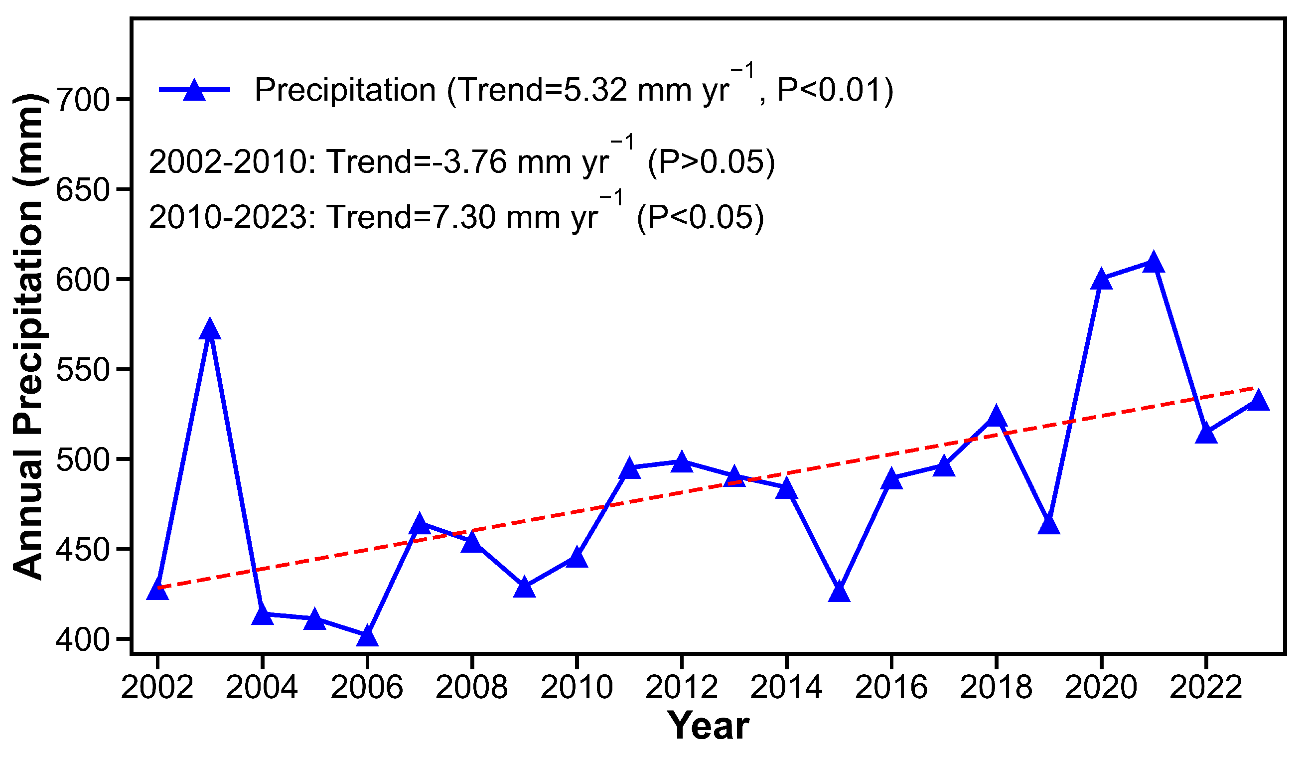
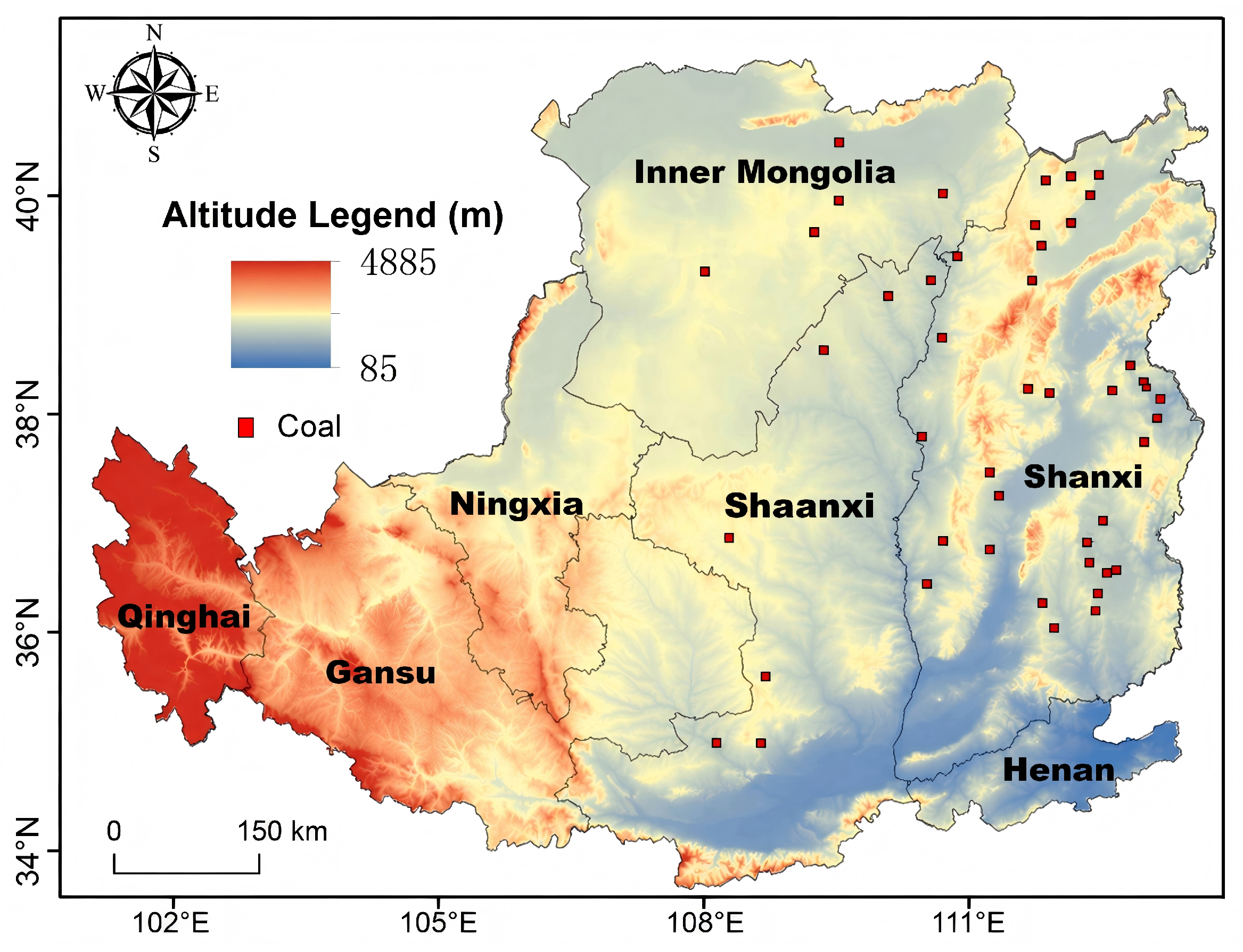
The LP is located in the middle reaches of the Yellow River Basin in northern China ( 33 ° 43 41 ° 16 N, 100 ° 54 114 ° 33 E), spanning Shaanxi, Shanxi, Gansu, Ningxia, Henan, Inner Mongolia, and Qinghai Provinces or Autonomous Regions, with a total area of approximately 6.4 × 10 5 km2 [30]. The region lies in a climatic transition zone from arid and semi-arid to sub-humid conditions, with a mean annual precipitation of approximately 483 mm (Figure 2). Precipitation is mainly concentrated in summer and exhibits strong seasonality [31,32]. Topographically, the study area generally has higher elevations in the northwest and lower elevations in the southeast, with highly complex landforms (Figure 3). Thick and continuous loess deposits, together with well-developed vertical joints, create complex linkages among surface ecological water consumption, SM infiltration, and deep hydrological processes.
Since the implementation of the GGP in 1999, the LP has undergone substantial vegetation restoration. Meanwhile, the region is also an important energy base and agricultural production area in China. Coal resources are abundant in northern Shaanxi, Shanxi, and southern Inner Mongolia, while irrigated agriculture is concentrated in the Fenwei Plain and along major river valleys. Therefore, the LP provides an important setting for examining long-term carbon–water coupling and its regional associations with groundwater storage and human water-use patterns.

2.2. Datasets

This study integrated satellite remote sensing products, land-surface assimilation data, satellite gravimetry, and socio-economic information to examine surface carbon–water dynamics and regional groundwater storage during 2002–2023 (Table 1). Monthly GPP and ET were aggregated to calendar-year values from January to December. Seven ET products—PML-V2, GLEAM, GLDAS, MOD16, SSEBop, ERA5-Land, and TerraClimate—were used for regional intercomparison and consistency assessment. Each product was converted from its native monthly units to annual ET, clipped to the LP boundary, and spatially averaged to obtain a regional annual time series. The multi-product average was calculated as the arithmetic mean of the available regional annual ET values across products for each year. The comparison was conducted among regional time series; no pixel-level ensemble averaging, fusion, or validation against independent flux observations was performed.
PML-V2 was used for the subsequent GPP–ET–WUE analysis because it provides GPP and ET within the same model framework, spatial grid, and temporal coverage. This internal consistency avoids combining incompatible GPP and ET products when calculating WUE, but it also means that the estimated WUE trend inherits the model structure, forcing assumptions, and uncertainties of PML-V2. Annual GPP, ET, and WUE in the main analysis therefore represent product-based calendar-year estimates.
The predictor variables used in the XGBoost–SHAP analysis were LAI, precipitation, air temperature, vapor pressure deficit (VPD), shortwave radiation (Rs), shallow SM, deep SM, and IWU. LAI was derived from MODIS [33]; precipitation, temperature, VPD, and Rs were obtained from TerraClimate [34]; and SM was obtained from GLDAS [35]. IWU was obtained from the 500 m national irrigation water-use dataset developed by the Aerospace Information Research Institute, Chinese Academy of Sciences [36]. Because IWU is available only for 2004–2019, all XGBoost–SHAP models that include IWU were restricted to this period. The years 2002–2003 and 2020–2023 were excluded only from IWU-related modeling; the long-term trend analyses of GPP, ET, WUE, SM, TWSA, and GWSA covered 2002–2023.
Table 1. Datasets used in this study.
AbbreviationsDatasetsSpatial ResolutionTemporal ResolutionData RangeData SourceReference
PML-V2PML-V2 ET500 mMonthly2002–2023https://developers.google.com/earth-engine/datasets/catalog/projects_pml_evapotranspiration_PML_OUTPUT_PML_V22a (accessed on 7 January 2026)Zhang et al. (2019) [37]
PML-V2PML-V2 GPP500 mMonthly2002–2023https://developers.google.com/earth-engine/datasets/catalog/projects_pml_evapotranspiration_PML_OUTPUT_PML_V22a (accessed on 7 January 2026)Zhang et al. (2019) [37]
GLEAMGLEAM ET 0.25 ° Monthly2002–2023https://www.gleam.eu/ (accessed on 20 December 2025)Martens et al. (2017) [38,39]
MODISMODIS ET and LAI500 mMonthly2002–2023https://lpdaac.usgs.gov/products/mod16a2v061/ (accessed on 11 December 2025)Mu et al. (2011) [33]
SSEBopSSEBop ET1 kmMonthly2002–2023https://earlywarning.usgs.gov/fews/ (accessed on 15 December 2025).Senay et al. (2013) [40]
ERA5-LandERA5-Land ET 0.1 ° Monthly2002–2023https://cds.climate.copernicus.eu/datasets/reanalysis-era5-land-monthly-means (accessed on 18 December 2025)Muñoz-Sabater et al. (2021) [41]
TerraClimateTerraClimate ET, VPD, Precipitation, Temperature, and Rs4 kmMonthly2002–2023https://www.climatologylab.org/terraclimate.html (accessed on 18 December 2025)Abatzoglou et al. (2018) [34]
GLDASGLDAS ET, SMSA, SWEA, CWSA, and SWSA 0.25 ° Monthly2002–2023https://ldas.gsfc.nasa.gov/gldas/gldas-get-data (accessed on 18 December 2025)Rodell et al. (2004) [35]
GRACETWSA 0.25 ° Monthly2002–2023https://grace.jpl.nasa.gov/data/get-data/jpl_global_mascons/ (accessed on 25 December 2025); https://www2.csr.utexas.edu/grace/RL06_mascons.html (accessed on 25 December 2025)Tapley et al. (2004) [42]
IWUIrrigation Water500 mYearly2004–2019https://zenodo.org/records/18906513 (accessed on 31 May 2026)Bo et al. (2026) [36]
Provincial Data on Human Water UseProvincialYearly2002–2023https://slt.shanxi.gov.cn/zwgk/fdzdgknr/gbxx/szygb/ (accessed on 24 May 2026); https://slt.shaanxi.gov.cn/zfxxgk/fdzdgknr/zdgz/szygb/ (accessed on 24 May 2026); https://slt.gansu.gov.cn/slt/c106726/c106732/c106773/c106775/tld.shtml (accessed on 24 May 2026); https://slt.nmg.gov.cn/xxgk/zfxxgkzl/fdzdgknr/gbxx/szygb/202508/t20250828_2781070.html (accessed on 24 May 2026)
Monthly GWSA was estimated from GRACE/GRACE-FO Level-3 Mascon products and GLDAS-Noah water-storage components. Two independent TWSA solutions from the University of Texas Center for Space Research (CSR; https://www2.csr.utexas.edu/grace/RL06_mascons.html (accessed on 25 December 2025)) and the NASA Jet Propulsion Laboratory (JPL; https://grace.jpl.nasa.gov/data/get-data/jpl_global_mascons/ (accessed on 25 December 2025)) were processed separately. Their agreement was used as a product-sensitivity check rather than as independent field validation. GLDAS-Noah L4 monthly data at 0.25 ° × 0.25 ° supplied SM, canopy-water, snow-water-equivalent, and surface-water-storage components [14]. All components were converted into anomalies relative to the 2004–2009 climatology, consistent with the GRACE reference period.
This study did not incorporate flux-tower or lysimeter ET observations, in situ soil-moisture records, or monitoring-well groundwater observations for direct field validation. Accordingly, the multi-product ET comparison and the CSR–JPL comparison were treated as cross-product consistency and product-sensitivity checks, respectively, while GLDAS SM and GRACE/GLDAS GWSA were interpreted as product-based regional estimates rather than site-validated measurements. This validation scope was considered explicitly when interpreting the regional trends and their uncertainties.
Provincial human water-use statistics were obtained from the water-resource bulletins of Gansu, Inner Mongolia, Shanxi, and Shaanxi and included agricultural, industrial, domestic, and ecological sectors. These four units cover a large proportion of the LP and include major irrigation and energy-development areas. Nevertheless, their administrative boundaries do not coincide exactly with the natural LP boundary, which also includes parts of Ningxia, Henan, and Qinghai. Province-wide totals were therefore used only to describe broad regional water-use context and were not treated as an LP water budget.

2.3. Methods

2.3.1. Estimation of GWSA Based on GRACE and GLDAS

TWSA derived from GRACE/GRACE-FO represents the combined variation in surface water, SM, snow-water equivalent, canopy-interception water, and groundwater within the satellite footprint. GWSA was estimated monthly by subtracting the non-groundwater components provided by GLDAS-Noah from TWSA, as shown in Equation (1):
GWSA = TWSA SMSA SWEA CWSA SWSA ,
where GWSA denotes groundwater storage anomaly, TWSA denotes terrestrial-water storage anomaly, SMSA denotes soil-moisture storage anomaly, SWEA denotes snow-water-equivalent anomaly, CWSA denotes canopy-interception-water storage anomaly, and SWSA denotes surface-water-storage anomaly. All variables are expressed in millimeters of water equivalent. SWEA was retained in the residual calculation even though snow storage is generally smaller than SM storage over much of the semi-arid LP, so that seasonal snow variability was not assigned to groundwater.
Because GWSA is a residual, uncertainties in both GRACE/GRACE-FO TWSA and GLDAS water-storage components accumulate in the groundwater estimate. CSR-derived GWSA and JPL-derived GWSA were therefore calculated separately, and the spread between their trend estimates was used as an indicator of product sensitivity. Provider-specific Mascon processing and scaling conventions were retained; no post hoc adjustment was used to force agreement between CSR and JPL data. Signal leakage across the LP boundary, the coarse effective GRACE footprint, differences in Mascon solutions, and uncertainties in GLDAS components were considered when interpreting trend magnitude. Missing months during the GRACE/GRACE-FO transition were linearly interpolated before annual aggregation. This treatment preserves a continuous annual series but may smooth short-term variability.

2.3.2. Statistical Analysis

The long-term trend of each variable was estimated using Sen’s slope [43], and significance was assessed with the nonparametric Mann–Kendall test [44]. GPP, ET, WUE, and human water-use variables were analyzed using calendar-year values; monthly SM, TWSA, and GWSA were first aggregated to annual means. Sen’s slope was calculated from annual observations. The standard Mann–Kendall test was applied without pre-whitening; annual aggregation reduces high-frequency dependence but does not guarantee temporal independence. Accordingly, p-values were interpreted together with slope magnitude and temporal pattern, rather than as the sole evidence for hydrological transition.
We used the following periods only for descriptive subperiod comparisons based on the observed annual trajectories: 2002–2010 and 2010–2023 for GPP, ET, and WUE; 2002–2015 and 2016–2023 for SM; and 2002–2020 and 2020–2023 for GWSA. These periods were not identified by a formal change-point test and are not presented as statistically detected breakpoints. In particular, the 2020–2023 GWSA increase is described as a short-term, nonsignificant fluctuation rather than stable long-term recovery.

2.3.3. Relative Growth Rate

To compare GPP and ET despite their different units and magnitudes, the relative growth rate (RGR) was calculated as Sen’s slope ( β ) divided by the multi-year mean ( X ¯ ):
RGR = β X ¯ × 100 % .
The RGR was used only as a normalized descriptive comparison to clarify whether the WUE increase reflected faster GPP growth or a decline in ET. It does not provide an independent ecological mechanism beyond the underlying GPP and ET trends.

2.3.4. Cross-Scale Comparison and Interpretation

The datasets used in the groundwater-related comparison differ substantially in spatial support, temporal coverage, and process representation. GPP, ET, WUE, and IWU resolve sub-kilometer-to-kilometer-scale surface variation; GRACE/GRACE-FO integrates water-storage changes over much broader footprints; provincial statistics follow administrative boundaries; and coal-resource maps indicate broad resource zones rather than mine-level drainage. Therefore, comparisons involving GWSA, irrigation, provincial water use, and coal resources were interpreted as regional temporal or spatial correspondence. To provide a concise quantitative description of the surface–groundwater mismatch without disaggregating GRACE to 500 m, mean GPP and ET were summarized over 233 common groundwater-scale grid cells. The Spearman rank correlation coefficient ( ρ ) was used to measure the strength and direction of the monotonic association between GWSA-decline intensity and mean GPP or ET; ρ ranged from 1 to 1, with values closer to zero indicating weaker monotonic association. The corresponding p-value denoted the two-sided probability of obtaining a correlation at least as extreme as the observed value under the null hypothesis of no monotonic association, and p < 0.05 was considered statistically significant.
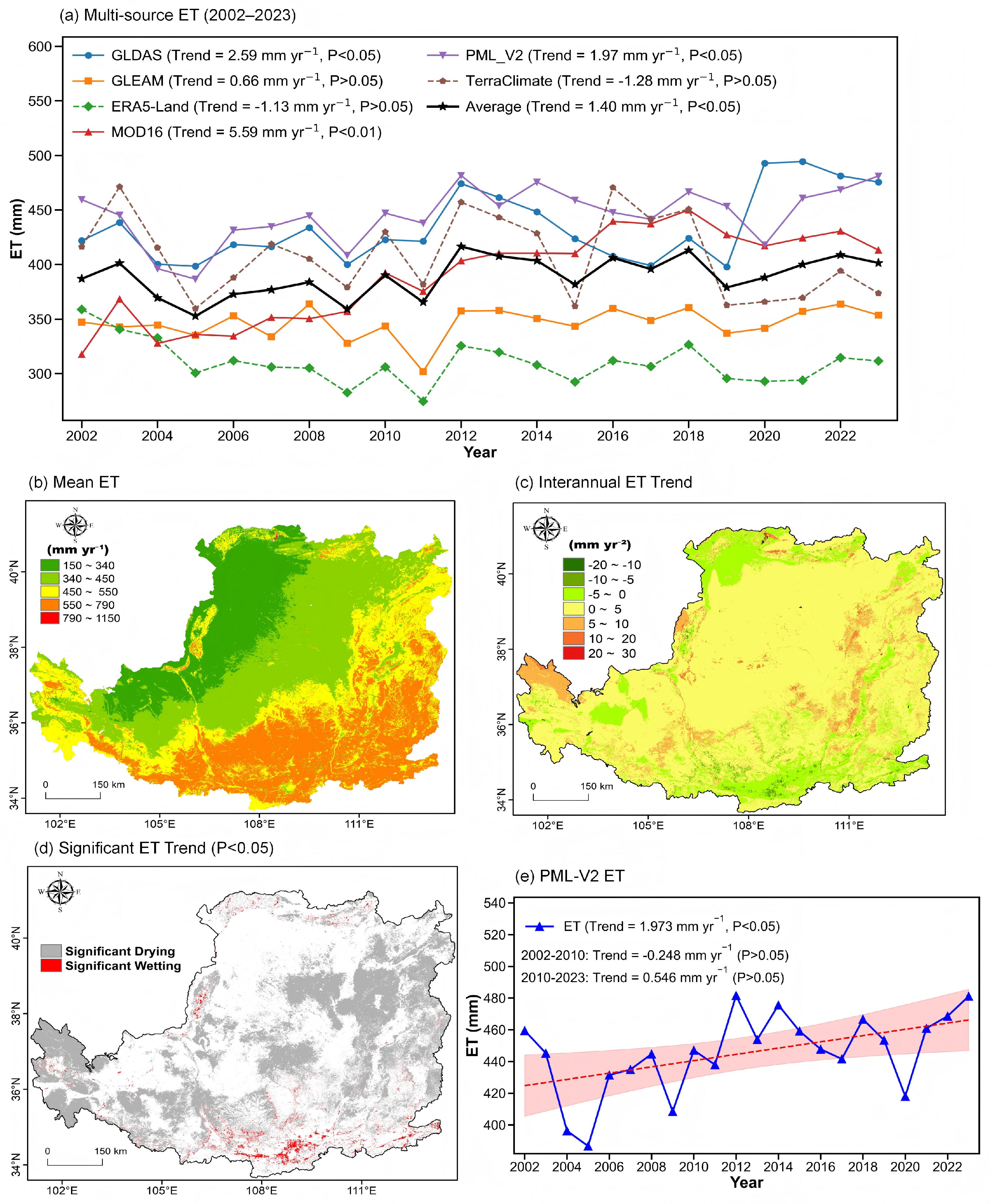
To complement the threshold-free domain-wide rank correlations, a zonal overlap-area analysis was performed on the same 233 common groundwater-scale grid cells. The thresholds were tied to the existing spatial-map classifications rather than optimized against the GWSA pattern. The GPP and ET high-value zones were defined using the lower boundaries of the two uppermost classes in their respective mean-value maps (Figure 4a and Figure 5b), corresponding to a mean GPP 1200 g C m−2 yr−1 and a mean ET 550 mm yr−1. These cutoffs therefore identify map-defined upper-value zones and are not interpreted as ecological or hydrological tipping points. For GWSA, a trend of 9 mm yr−1 was used as the reference definition of strong decline. This cutoff is close to the observed regional long-term GWSA trend magnitude ( 9.131 mm yr−1) and corresponds to a class boundary in the mapped GWSA trend, thereby identifying cells declining at approximately the regional long-term rate or faster. For the strong-GWSA-decline zone S and a map-defined GPP or ET high-value zone H, the overlap rate and Jaccard index were calculated as
O = A ( S H ) A ( S ) × 100 % , J = A ( S H ) A ( S H ) ,
where A ( · ) denotes the total area of the corresponding common-grid zone. The overlap rate measures the proportion of the strong groundwater-decline zone coinciding with a high-value surface zone, whereas the Jaccard index measures the overall similarity between the two spatial sets. Because overlap metrics are inherently threshold-dependent, they were interpreted together with the continuous Spearman correlations rather than as stand-alone evidence. The thresholds were used only to provide a transparent and reproducible descriptive classification and were not used for causal attribution.

2.3.5. XGBoost–SHAP Analysis of Model-Based Associations

All XGBoost–SHAP analyses were implemented in Python (version 3.9.23) using XGBoost (version 2.1.4), SHAP (version 0.49.1), and scikit-learn (version 1.6.1). XGBoost regression models were constructed separately for GPP, ET, and WUE to characterize their model-based associations with vegetation, climatic, soil-moisture, and irrigation-related variables [45]. The predictors included LAI, precipitation, air temperature, VPD, Rs, shallow SM, deep SM, and IWU. These models were developed to explain variations in surface-ecosystem carbon–water variables and were not used to attribute changes in GWSA.
All predictor and response variables were aggregated to calendar-year values over the common period of 2004–2019. For each response variable, its raster grid was used as the reference grid, and the predictor rasters were reprojected, clipped, and co-registered to that grid before pixel extraction. This alignment produced co-located annual raster stacks but did not alter the native effective spatial support of the coarser predictors; aligned fine-grid cells derived from a coarse product were therefore not treated as independent fine-resolution observations. For IWU, non-irrigated areas and pixels with missing or negative values were assigned a value of zero after spatial alignment.
Pixels containing missing or infinite values, non-positive response values, non-positive LAI, negative precipitation, or negative IWU were excluded. For the WUE model, values outside the predefined range of 0 < WUE < 10 were additionally removed to reduce the influence of extreme values. Up to 10,000 valid pixels were randomly sampled from each year using a fixed random seed of 42, yielding a maximum possible sample size of 160,000 observations for each model before quality-control losses.
Three validation strategies were implemented. First, the pooled samples were randomly divided into training and test subsets in an 80:20 ratio using a random seed of 42. This random split was retained only as a baseline because spatially adjacent pixels and repeated observations from different years may not be statistically independent. Second, five-fold spatial block cross-validation was conducted as the primary assessment of model performance. Pixel-center coordinates were transformed into the equal-area coordinate system EPSG:6933 and assigned to fixed 100 × 100 km spatial blocks. All observations within the same spatial block, including observations from different years, were assigned exclusively to either the training or test subset in each fold, thereby reducing information leakage between spatially adjacent samples. Third, leave-one-year-out validation was conducted to evaluate temporal stability. Each year from 2004 to 2019 was successively used as an independent test set, while observations from the remaining 15 years were used for model training.
All three models used the same fixed XGBRegressor settings: n_estimators = 400, max_depth = 6, learning_rate = 0.05, subsample = 0.8, colsample_bytree = 0.8, objective = reg:squarederror, n_jobs = −1, and random_state = 42. No separate hyperparameter optimization or early-stopping procedure was applied. The same parameter settings were retained for GPP, ET, and WUE to ensure methodological comparability.
Model performance was evaluated using the standard regression coefficient of determination ( R 2 ) and root mean square error (RMSE):
R 2 = 1 i = 1 N ( y i y ^ i ) 2 i = 1 N ( y i y ¯ ) 2 ,
RMSE = 1 N i = 1 N ( y i y ^ i ) 2 ,
where y i and y ^ i are the observed and predicted values, respectively; y ¯ is the mean of the observed values; and N is the number of test samples. Higher R 2 and lower RMSE indicate better predictive performance. For spatial block cross-validation, the mean and standard deviation of each metric were calculated across the five folds. For leave-one-year-out validation, the corresponding statistics were calculated across the 16 independently held-out years. Spatial block cross-validation was used as the primary measure of model performance, whereas the random split and leave-one-year-out validation were used as baseline and temporal-stability assessments, respectively.
SHAP values were calculated using a tree-based explainer to characterize the contribution of each predictor within the fitted models. To reduce the influence of spatial information leakage on model interpretation, SHAP values were calculated separately for the spatially held-out test samples in each cross-validation fold. Test samples from the five folds were pooled to generate the SHAP summary plots and global feature-importance percentages. Mean absolute SHAP values were used to rank predictor importance, while the distributions of signed SHAP values were used to describe the direction and variability of the model-based associations. The reported SHAP results therefore represent out-of-fold associations evaluated on spatially independent test samples rather than explanations derived solely from a random train–test split. SHAP values quantify predictor contributions within the fitted models and do not demonstrate that an individual predictor was independently responsible for changes in GPP, ET, or WUE.

3. Results

3.1. Marked Increase in Vegetation Productivity Under Ecological Restoration

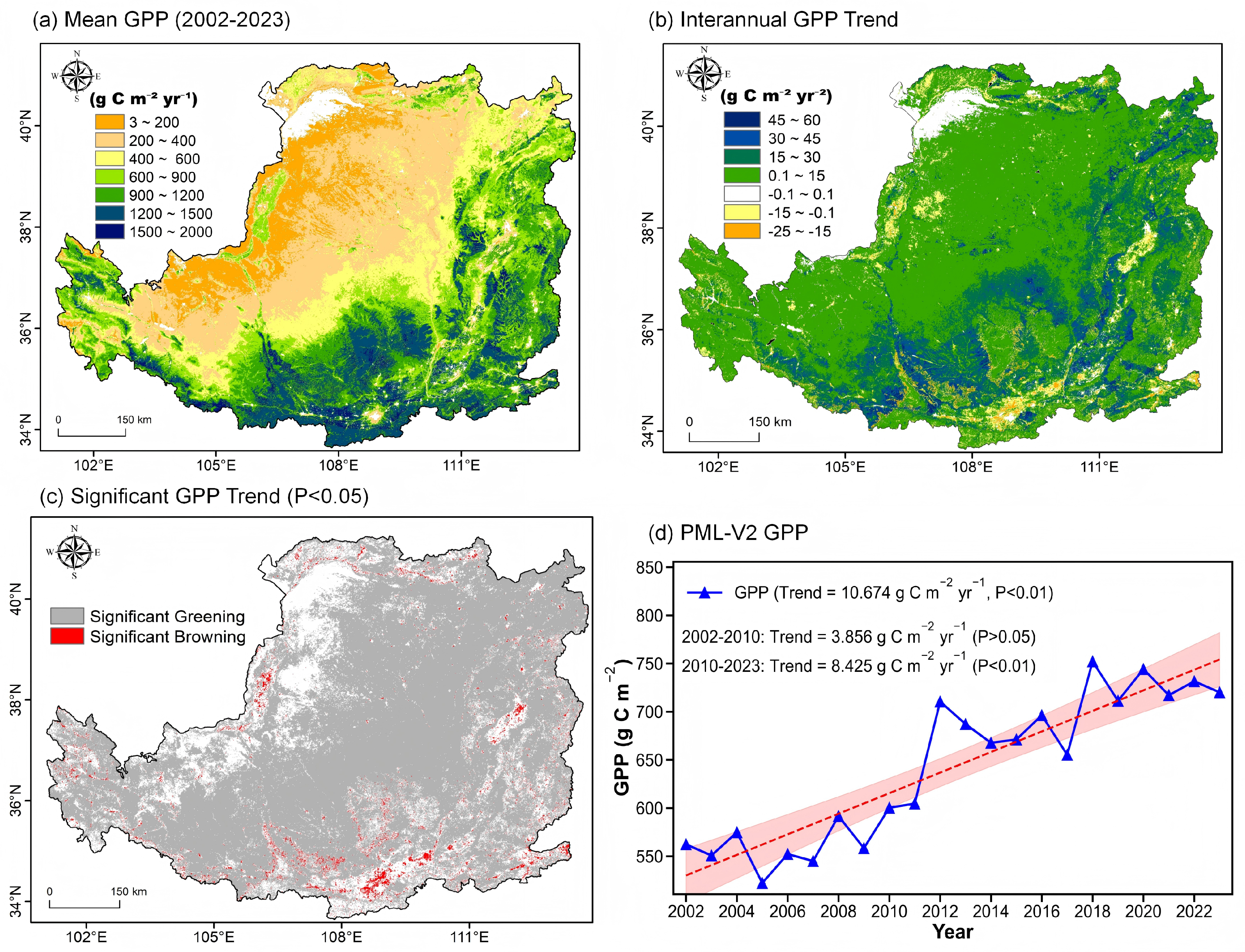
From 2002 to 2023, GPP across the LP exhibited a significant increasing trend (Figure 4d). The regional mean annual GPP was 642.13 g C m−2, with a maximum of 752.16 g C m−2 in 2018 and a minimum of 522.14 g C m−2 in 2005. Sen’s slope was 10.67 g C m−2 yr−1 ( p < 0.01 ). Descriptive subperiod analysis showed increases of 3.86 g C m−2 yr−1 during 2002–2010 ( p > 0.05 ) and 8.42 g C m−2 yr−1 during 2010–2023 ( p < 0.01 ), indicating that the regional productivity increase was more persistent in the later period.
The long-term mean GPP showed a clear southeast–northwest decreasing gradient (Figure 4a). High GPP values occurred mainly in southeastern Shaanxi, southern Shanxi, western Henan, and the mountainous forest–shrub regions of southeastern Gansu, whereas low values were concentrated in southern Inner Mongolia, northern Ningxia, and northwestern Gansu. Increasing GPP occurred across 91.17% of the study area, with 77.26% showing significant increases; decreasing GPP occurred across 6.44% of the study area, with 2.35% showing significant decreases (Figure 4b,c). These spatial and temporal patterns document a widespread productivity increase during the ecological-restoration period.

3.2. ET Increased More Modestly than GPP

3.2.1. Intercomparison of Multi-Source ET Products

Multiple ET datasets were compared to assess the consistency of long-term regional trends and reduce dependence on any single land-surface model or remote sensing algorithm. Although the products differed in absolute magnitude and interannual variability, they consistently indicated only a small long-term increase from 2002 to 2023 (Figure 5a). The multi-product average regional ET series showed a Sen’s slope of 1.40 mm yr−1, indicating a small positive tendency, although its magnitude remained uncertain.

3.2.2. Temporal and Spatial Patterns of ET

Based on PML-V2, the mean annual ET was 420.57 mm, with a maximum of 481.11 mm in 2012 and a minimum of 386.66 mm in 2005. ET increased by 1.97 mm yr−1 during 2002–2023 ( p < 0.05 ). The descriptive subperiod slopes were −0.25 mm yr−1 during 2002–2010 ( p > 0.05 ) and 0.55 mm yr−1 during 2010–2023 ( p > 0.05 ), and neither subperiod showed a significant monotonic trend. Thus, the regional restoration period was not accompanied by a strong or temporally uniform increase in ET.
The long-term mean ET generally decreased from southeast to northwest (Figure 5b). High ET values occurred mainly in southern and southeastern Shaanxi, southeastern Shanxi, western Henan, southeastern Gansu, and localized mountainous areas in eastern Qinghai, whereas low values occurred mainly in southern Inner Mongolia, northern Ningxia, and northern Gansu. Increasing ET occurred across 84.43% of the LP, with 35.17% showing significant increases. Decreasing ET occurred across 15.56% of the study area, with 2.32% showing significant decreases (Figure 5c,d). The limited area of significant ET increase contrasts with the more spatially extensive GPP increase.

3.3. WUE Increase Was Primarily Associated with Faster GPP Growth

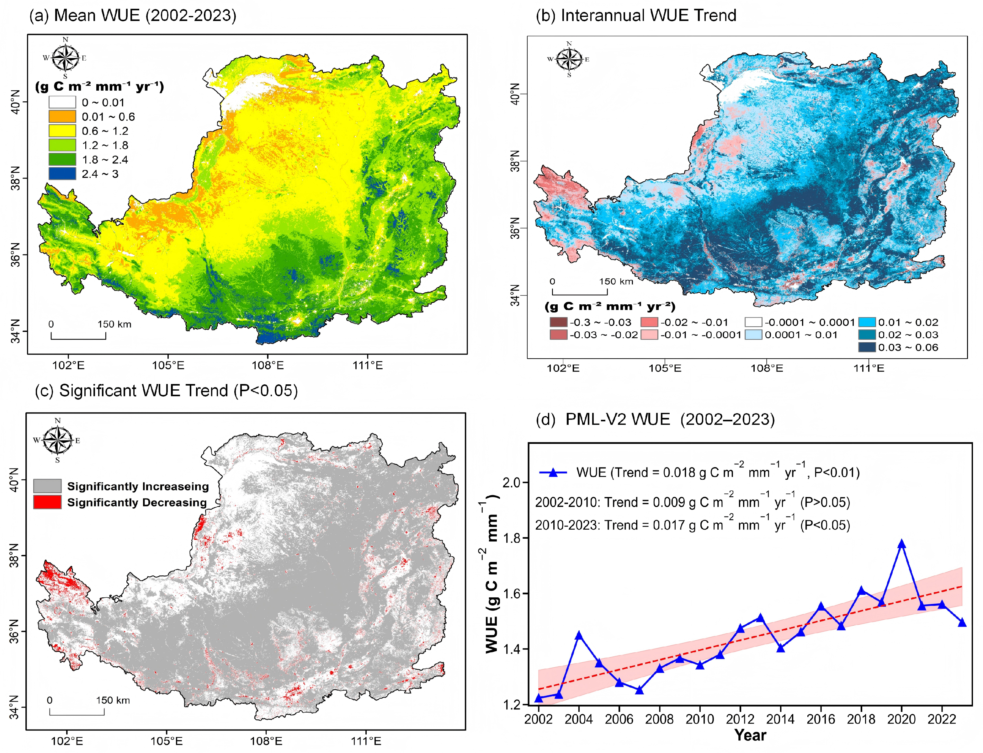
WUE exhibited a significant increasing trend from 2002 to 2023 (Figure 6d). The regional mean annual WUE was 1.44 g C m−2 mm−1, with the minimum in 2002 and the maximum in 2020. Sen’s slope was 0.018 g C m−2 mm−1 yr−1 ( p < 0.01 ). The descriptive subperiod increases were 0.009 g C m−2 mm−1 yr−1 during 2002–2010 ( p > 0.05 ) and 0.017 g C m−2 mm−1 yr−1 during 2010–2023 ( p < 0.05 ), indicating a clearer increase in the later period.
The long-term mean WUE showed a southeast-to-northwest decreasing gradient (Figure 6a), with high values concentrated in southeastern Shaanxi, Shanxi, western Henan, and southern mountainous and hilly areas. Increasing WUE occurred across 87.25% of the study area, with 67.35% showing significant increases. Decreasing WUE occurred across 10.35% of the study area, with 3.06% showing significant decreases (Figure 6b,c).
The relative growth rate of GPP was 1.66%, compared with 0.47% for ET. Because WUE is defined as GPP/ET, this faster relative increase in GPP provides the numerical basis for the observed WUE increase and shows that carbon gain rose more rapidly than ecosystem water consumption.

3.4. Model-Based Associations of Carbon–Water Variables

Model performance was assessed primarily using five-fold spatial block cross-validation. The mean R 2 values (mean ± standard deviation across folds) were 0.9089 ± 0.0172 for GPP, 0.8816 ± 0.0130 for ET, and 0.9144 ± 0.0156 for WUE. The mean RMSE values were 16.0249 g C m−2 yr−1 for GPP, 14.12 mm yr−1 for ET, and 0.1756 g C m−2 mm−1 for WUE. The random 80:20 split was retained only as a baseline, whereas leave-one-year-out validation was used as an auxiliary assessment of temporal stability. Spatial block cross-validation was used for the primary performance estimates because it reduced information leakage between neighboring raster samples. These metrics describe predictive performance under the specified validation schemes and should not be interpreted as evidence of causal relationships.
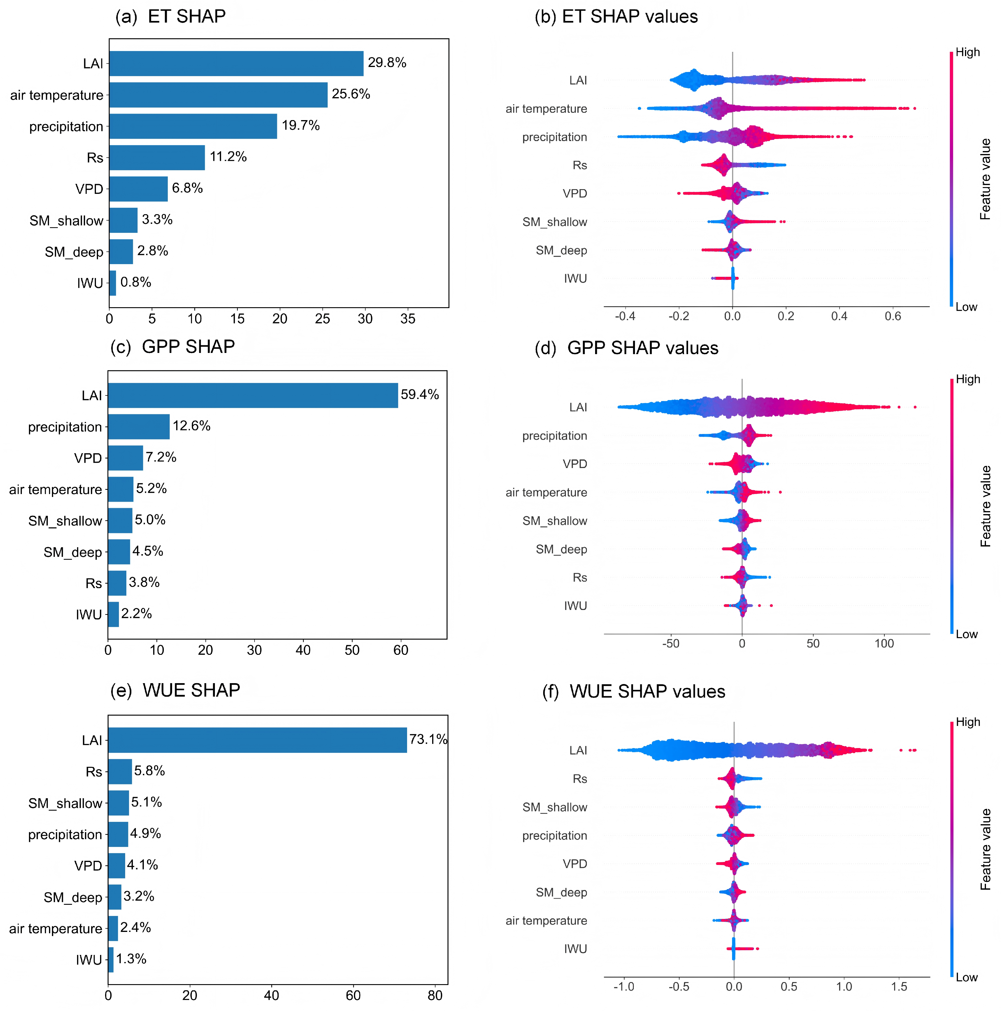
For GPP (Figure 7c,d), LAI made the largest global SHAP contribution (59.4%), followed by precipitation (12.6%), VPD (7.2%), air temperature (5.2%), shallow SM (5.0%), deep SM (4.5%), Rs (3.8%), and IWU (2.2%). High-LAI samples were mainly associated with positive SHAP values, whereas the other variables showed narrower SHAP distributions. These results identify LAI as the predictor most strongly associated with spatial and temporal variation in GPP within the fitted model.
For ET (Figure 7a,b), the largest SHAP contributions were associated with LAI (29.8%), air temperature (25.6%), and precipitation (19.7%). Rs, VPD, shallow SM, deep SM, and IWU contributed 11.2%, 6.8%, 3.3%, 2.8%, and 0.8%, respectively. The broader SHAP distributions of LAI, air temperature, and precipitation indicate that ET variation in the fitted model was associated with both vegetation conditions and hydroclimatic variability rather than with a single predictor.
For WUE (Figure 7e,f), LAI made the largest contribution (73.1%), followed by Rs (5.8%), shallow SM (5.1%), precipitation (4.9%), VPD (4.1%), deep SM (3.2%), air temperature (2.4%), and IWU (1.3%). High-LAI samples were mainly associated with positive SHAP values. The relative SHAP magnitudes describe model-based associations and do not establish that changes in any individual predictor independently produced the observed WUE trend.

3.5. Asynchronous Responses of SM and Regional GWSA

3.5.1. Temporal Variations in Soil Moisture Profiles and GWSA

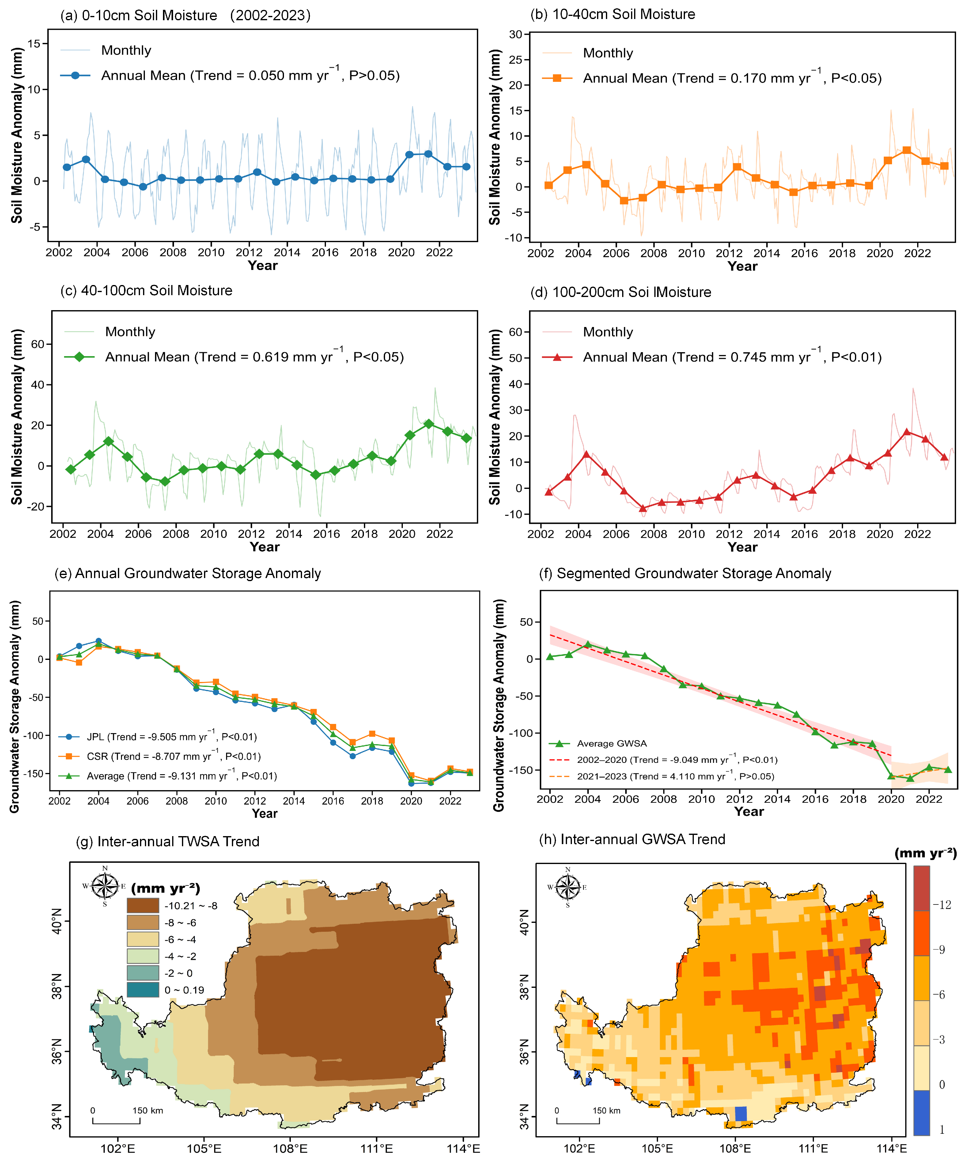
Soil-moisture anomalies showed pronounced interannual fluctuations and contrasting descriptive subperiod patterns at all four depths (Figure 8a–d; Table 2). During 2002–2015, the slopes at 0–10, 10–40, 40–100, and 100–200 cm were −0.068, −0.070, −0.206, and −0.346 mm yr−1, respectively. Although these slopes were not statistically significant, all were negative, and their magnitudes were larger in the deeper layers.
During 2016–2023, the slopes became positive at all depths. The 0–10 cm layer increased by 0.319 mm yr−1 ( p > 0.05 ), while the 10–40, 40–100, and 100–200 cm layers increased by 0.891, 2.999, and 2.190 mm yr−1, respectively ( p < 0.05 ). The later period was therefore characterized by recovery in middle and deep soil moisture. In contrast, the CSR- and JPL-derived GWSA series both showed significant long-term declines (Figure 8e). The CSR slope was −8.707 mm yr−1, and the JPL slope was −9.505 mm yr−1. The averaged CSR–JPL GWSA series showed a Sen’s slope of −9.131 mm yr−1 ( p < 0.01 ). GWSA showed a slope of −9.049 mm yr−1 during 2002–2020 ( p < 0.01 ) and a short-term, nonsignificant increase of 4.110 mm yr−1 during 2020–2023 ( p > 0.05 ) (Figure 8f). Thus, the increasing tendency in middle and deep soil moisture during 2016–2023 was not accompanied by a corresponding long-term increase in regional groundwater storage. The SM anomaly trends describe changes in soil-water storage state rather than direct groundwater-recharge fluxes. Because the available datasets do not provide LP-wide time series of irrigation-related groundwater abstraction or mine-drainage discharge, the contrast between SM and GWSA cannot be used as a quantitative water-balance demonstration that soil-water recharge was smaller than anthropogenic groundwater withdrawal.

3.5.2. Spatial Patterns of TWSA and GWSA

TWSA and GWSA both showed predominantly decreasing spatial trends across the LP (Figure 8g,h). The decline was generally weaker in the western and southwestern LP, including eastern Qinghai and western Gansu, and stronger in central-northern Shaanxi, eastern and southern Inner Mongolia, and Shanxi. This pattern differed from the southeast–northwest gradients of mean GPP, ET, and WUE. The common-grid quantitative analysis further showed weak and nonsignificant correlations between GWSA-decline intensity and mean GPP (Spearman’s ρ = 0.092 , p = 0.162 ) or mean ET ( ρ = 0.091 , p = 0.166 ). Using the map-defined reference thresholds described in Section 2.3.4, the zonal overlap-area analysis showed that 16.9% of the strong-GWSA-decline zone overlapped with the GPP high-value zone and that 31.0% overlapped with the ET high-value zone; the corresponding Jaccard indices were 0.095 and 0.129, respectively (Table 3). The conclusion of limited spatial agreement is therefore supported by two complementary forms of evidence: a threshold-free continuous rank correlation analysis and a threshold-based zonal overlap analysis. The overlap values are interpreted as descriptive agreement under the stated classification rules rather than as universal hotspot boundaries or evidence of causality.

3.6. Regional Human Water-Use Context for GWSA Interpretation

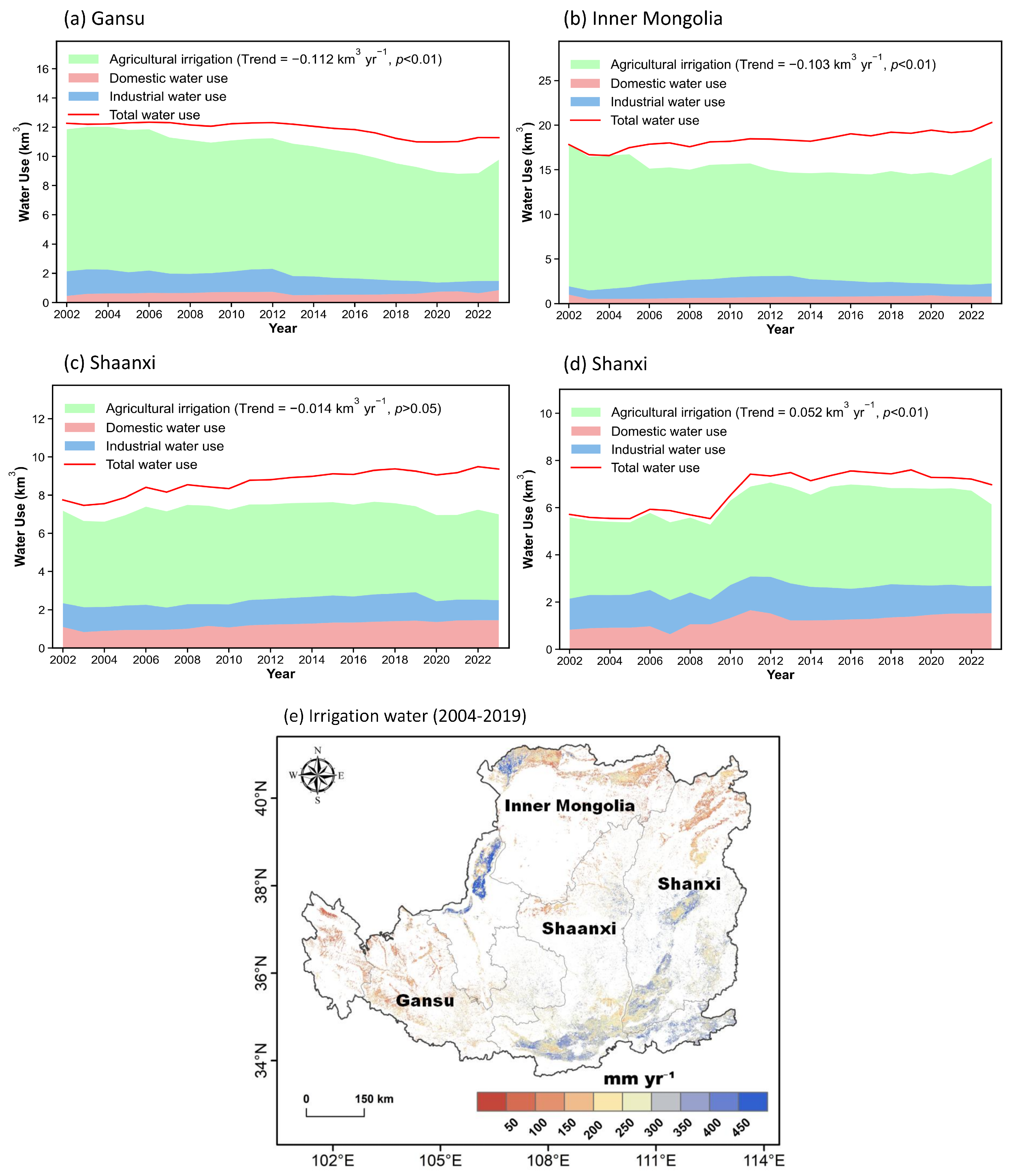
Provincial water-resource bulletins showed that agricultural irrigation remained the largest water-use sector in Gansu, Inner Mongolia, Shanxi, and Shaanxi during 2002–2023 (Figure 9a–d). Mean irrigation use was 12.97 km3 in Inner Mongolia, and it was 8.77 km3 in Gansu, with significant decreasing trends of −0.103 and −0.112 km3 yr−1, respectively ( p < 0.01 ). Mean irrigation use was 3.72 km3 in Shanxi, with a significant increase of 0.052 km3 yr−1 ( p < 0.01 ), and it was 4.81 km3 in Shaanxi, with no significant trend (−0.014 km3 yr−1, p > 0.05 ). Because these values represent entire provinces rather than only the portions within the LP, they describe broad water-use context rather than an LP water budget.
The 500 m IWU dataset for 2004–2019 showed strong spatial heterogeneity (Figure 9e). High values occurred mainly in eastern and southeastern plains, river valleys, and agricultural areas near the Shanxi–Shaanxi–Henan junction, whereas most upland and northwestern areas had low values. The strongest GWSA declines were concentrated farther north in Shanxi, central-northern Shaanxi, and southern Inner Mongolia. The spatial correspondence was therefore limited, and the qualitative spatial comparison indicated only broad contextual similarity rather than complete spatial agreement.
Northern Shanxi, northern Shaanxi, and southern Inner Mongolia are also major coal-resource regions (Figure 3). Some spatial correspondence can be observed between these broad resource zones and areas of marked GWSA decline (Figure 8h). This qualitative spatial comparison provides only broad contextual similarity for considering mine drainage and energy-related water use [46]; the coal-resource map does not contain mine-specific drainage volumes or aquifer responses and cannot support a quantified mining contribution.
Neither the provincial water-use statistics nor the coal-resource map provides a spatially explicit time series of groundwater abstraction or mine-drainage discharge within the LP. These datasets were therefore not used to calculate anthropogenic groundwater withdrawal, to quantitatively compare withdrawal with soil-water recharge, or to infer that anthropogenic extraction exceeded recharge.

4. Discussion

4.1. Ecological Restoration Was Accompanied by Enhanced Carbon Gain and WUE

The dominant surface-ecosystem signal during 2002–2023 was a widespread increase in vegetation productivity. Regional GPP increased at a rate of 10.67 g C m−2 yr−1, and significant increases occurred across 77.26% of the LP. This spatially extensive increase is consistent with the long-term greening and improvement in ecosystem functioning reported following the implementation of the GGP [5,6,7]. WUE also increased significantly across most of the study area, indicating that greater carbon gain per unit of water consumed occurred in the context of ecological restoration.
The increase in WUE should not, however, be interpreted as a reduction in total ecosystem water loss, because both GPP and ET exhibited positive trends. Instead, the relative growth rate of GPP was 1.66%, substantially greater than the 0.47% relative growth rate of ET. This contrast indicates that the improvement in WUE was primarily associated with a faster increase in carbon gain rather than with declining ET. The RGR was used only to place the trends in GPP and ET on a common relative scale and to facilitate comparison between variables with different units and magnitudes.
The XGBoost–SHAP results provided complementary model-based evidence for these patterns. LAI made the largest mean absolute SHAP contribution to both GPP and WUE, consistent with the close association of canopy development and vegetation structure with ecosystem productivity and carbon–water coupling [47,48]. Nevertheless, LAI also covaries with restoration history, vegetation type, climate, and site conditions. Its high SHAP importance should therefore be interpreted as a strong association within the fitted models rather than as evidence of an isolated causal pathway.

4.2. Carbon Gain Increased Faster than Ecosystem Water Consumption

The multi-product ET intercomparison showed a generally weak positive regional trend, although the products differed considerably in their absolute ET estimates. PML-V2 ET increased at a rate of 1.97 mm yr−1, and significant increases occurred across only 35.17% of the LP. More importantly, the relative increase in ET was substantially smaller than that in GPP. These results show that the pronounced increase in ecosystem carbon gain was not accompanied by a proportional increase in annual ET at the regional scale. This difference provides the direct basis for the observed increase in WUE.
This regional annual pattern does not imply that ecological restoration had no effect on water cycling. Localized or seasonal increases in transpiration, canopy interception, and root water uptake may still have occurred, and vegetation change may also have indirectly influenced infiltration, groundwater recharge, and subsurface flow. Therefore, the slower regional increase in ET should be interpreted as evidence against a simple one-to-one relationship between vegetation recovery and annual ecosystem water consumption, rather than as evidence of an absence of ecohydrological effects [49,50].
Within the ET model, LAI, air temperature, and precipitation made the largest mean absolute SHAP contributions, indicating that annual ET variability was jointly associated with vegetation conditions and hydroclimatic variability. Although VPD contributed less than LAI, this result does not indicate that atmospheric water demand was ecophysiologically unimportant. At the annual scale, VPD may contain information that overlaps with air temperature and precipitation, and its association with ET may vary nonlinearly with vegetation status and soil-water availability. In addition, tree-based models may redistribute importance among correlated predictors. The SHAP ranking therefore represents the relative contribution of each predictor within the fitted model, rather than a universal hierarchy of the ecohydrological factors controlling ET [49,50].

4.3. Surface Carbon–Water Recovery Did Not Translate into Synchronous Groundwater Recovery

The most important cross-system finding was the asynchronous response between surface-ecosystem carbon–water processes and deep groundwater storage. During 2002–2023, GPP and WUE increased markedly, whereas ET increased at a substantially slower relative rate. Middle- and deep-layer SM also showed an increasing tendency during the descriptive 2016–2023 period. In contrast, both CSR- and JPL-derived GWSA exhibited pronounced declines through 2020, followed only by a short-term, nonsignificant increase during 2020–2023. The broad groundwater decline is consistent with previous GRACE-based assessments of groundwater stress across the LP [14,16,17,18]. This temporal contrast was accompanied by weak, nonsignificant spatial correlations ( ρ 0.09 ) and low Jaccard indices (0.095–0.129) between GWSA decline and high GPP or ET. Together, the temporal and spatial evidence indicates that increases in vegetation productivity and WUE, together with improvements in soil-water conditions, were not accompanied by synchronous regional groundwater recovery.
This asynchronous pattern is not interpreted as a comparison between groundwater recharge and anthropogenic withdrawal. SM anomalies represent changes in soil-water storage rather than recharge fluxes, and this study lacks spatially compatible time series of groundwater pumping and mine drainage. Therefore, the analysis cannot determine whether recharge was quantitatively smaller than human groundwater extraction, and no such mass-balance conclusion is drawn.
This asynchrony provides a more direct answer to the central question of this study than an activity-specific attribution of groundwater decline. The faster increase in GPP than in ET shows that the ecological-restoration period was accompanied by greater carbon gain per unit of water consumed without a proportional increase in annual ecosystem water consumption. However, the continued decline in GWSA indicates that improved surface carbon–water performance did not translate directly into groundwater recovery at the regional scale. This finding does not imply that ecological restoration is hydrologically independent of groundwater. Vegetation change may still influence infiltration, recharge, rooting depth, preferential flow, and seasonal water partitioning, but these effects need not produce a one-to-one correspondence between annual surface-ecosystem responses and regional groundwater storage. The conclusion is therefore limited to asynchronous regional trajectories rather than the absence of ecological influences on groundwater processes.
Scale differences are important when interpreting the asynchronous changes in surface-ecosystem processes and groundwater storage. The 500 m surface datasets capture fine-scale spatial heterogeneity in vegetation restoration, ET, soil moisture, and irrigation, whereas GRACE/GRACE-FO represents water-storage signals integrated over much broader spatial footprints, potentially smoothing localized groundwater variations. Meanwhile, the complex hydrogeological conditions of the LP may produce contrasting groundwater responses among subregions. Therefore, the present results primarily indicate different regional trajectories of surface-ecosystem recovery and groundwater storage and should not be used to infer groundwater responses at specific sites or to specific human activities.

4.4. Human Water Use and Resource Development as Regional Context

Agricultural irrigation remained the largest water-use sector in the four selected provincial units, while the 500 m IWU dataset showed relatively high irrigation demand in plains, river valleys, and major agricultural areas. Some spatial correspondence was observed between areas of pronounced GWSA decline and intensive irrigation zones or coal-resource-rich regions. This qualitative spatial comparison indicates only broad contextual similarity and does not quantify the influence of agricultural water demand, industrial water use, or resource development on groundwater dynamics [46,51]. The correspondence was not uniform: some areas with high IWU did not exhibit the strongest groundwater decline, irrigation water may be supplied by either surface water or groundwater, and coal-resource distribution does not directly represent mining intensity or mine-drainage volumes. In addition, the province-level statistics follow administrative boundaries that do not coincide precisely with the LP boundary. These data should therefore be interpreted as regional background information rather than as quantitative estimates of groundwater withdrawal within the entire LP.
The XGBoost–SHAP models cannot directly resolve the contribution of these human activities to groundwater change because their response variables were GPP, ET, and WUE rather than GWSA. Although IWU accounted for less than 3% of the SHAP importance in the three surface carbon–water models, this result only indicates a limited association with the modeled surface-ecosystem variables. It neither confirms nor excludes an influence of irrigation-related groundwater abstraction. Likewise, spatial correspondence among GWSA decline, irrigation zones, and coal-resource-rich regions cannot establish the individual effects of irrigation or mining. The available evidence is therefore insufficient to rank hydroclimatic variability, agricultural and industrial water use, resource development, and water-management practices as independent factors controlling regional groundwater dynamics.
Accordingly, irrigation and coal-resource information are retained only as regional contextual datasets in this study. They are not used to estimate groundwater withdrawal, mine-drainage volumes, or the relative magnitude of anthropogenic withdrawal versus groundwater recharge.

4.5. Uncertainties, Scale Limitations, and Future Work

A central limitation is the absence of direct in situ validation. This study does not incorporate flux-tower or lysimeter ET observations, site-scale soil-moisture monitoring, or monitoring-well groundwater records. Consequently, the ET multi-product comparison and CSR–JPL GWSA comparison evaluate cross-product consistency and product sensitivity rather than field accuracy. The reported ET, SM, and GWSA changes should therefore be interpreted as regional, product-based estimates, and their applicability to individual sites or aquifers remains limited.
First, the ET products differ in algorithms, forcing data, units, and spatial resolution. Their regional agreement supports the direction of the small ET increase, but these products are used for intercomparison, not validation against flux towers or lysimeters. PML-V2 provides internally consistent GPP and ET, yet WUE inherits uncertainties from both variables. Annual uncertainty bands for GPP and WUE were not estimated from independent products, and the results should be regarded as product-dependent regional estimates.
Second, five-fold spatial block cross-validation and leave-one-year-out validation were implemented to reduce the dependence associated with random pixel splitting and to assess temporal stability. Nevertheless, these procedures do not eliminate all model uncertainty. The reported performance may still depend on the selected 100 × 100 km block size, fold allocation, annual sampling, and fixed hyperparameter settings. Co-registration of predictors with different native resolutions also does not create new independent fine-scale information, so the effective spatial support of the coarser climate and soil-moisture products should be considered when interpreting model performance and SHAP importance. In addition, the models were not repeatedly refitted under alternative block sizes or sampling seeds, and confidence intervals for SHAP feature importance were not calculated. The spatial block results should therefore be interpreted as the primary performance estimates under the adopted validation design, while the leave-one-year-out results provide an auxiliary temporal-stability check. Future work should examine repeated spatial cross-validation, alternative block definitions, and bootstrap-based SHAP uncertainty intervals.
Third, GWSA is a residual of GRACE/GRACE-FO TWSA and GLDAS-derived SMSA, SWEA, CWSA, and SWSA. Leakage across the LP boundary, provider-specific scaling, interpolation of missing months, and GLDAS uncertainty can all influence trend magnitude. CSR–JPL consistency provides a product-sensitivity check but not full uncertainty propagation or independent validation. Monitoring-well observations, aquifer-specific storage coefficients, alternative GLDAS products, and confidence intervals for GWSA trends are needed for stronger groundwater evaluation.
Fourth, the reported subperiods are descriptive windows rather than statistically detected breakpoints. The common-grid Spearman correlations, zonal overlap rates, and Jaccard indices provide a quantitative but still descriptive measure of the GPP/ET–GWSA mismatch. The GPP and ET cutoffs were based on the upper classes of the existing spatial maps, while the 9 mm yr−1 GWSA cutoff was selected as a transparent reference close to the regional long-term decline and to the mapped class boundary. This classification-based choice reduces post hoc tuning to the groundwater pattern, but the absolute overlap and Jaccard values remain conditional on the selected cutoffs. For this reason, the threshold-based metrics were interpreted jointly with the threshold-free Spearman correlations, and none of the thresholds was treated as a universal ecological or hydrological boundary. Provincial statistics extend outside the LP, IWU covers only 2004–2019, irrigation sources are mixed, and mine-level production and drainage data were unavailable. No quantitative activity-specific overlap analysis or GWSA attribution model was implemented for irrigation or mining. The absence of LP-wide groundwater-abstraction and mine-drainage time series also precludes a quantitative comparison between groundwater recharge and anthropogenic withdrawal. Future work should combine formal change-point analysis, hydrogeological subregionalization, spatially compatible groundwater observations, groundwater-abstraction records, mine-drainage data, and process-based modeling.

5. Conclusions

This study investigated whether increased ecosystem carbon gain in the context of ecological restoration was accompanied by a proportional increase in regional ecosystem water consumption and by synchronous changes in groundwater storage across the LP. The main conclusions are as follows:
(1)
During 2002–2023, GPP increased significantly, whereas ET showed a much weaker increase. The relative growth rate of GPP was 1.66%, approximately 3.5 times that of ET (0.47%), and WUE increased significantly across most of the LP. Thus, the dominant surface signal was an increase in carbon gain relative to ecosystem water consumption, rather than a proportional increase in annual ET.
(2)
For the common period of 2004–2019, the XGBoost–SHAP models identified LAI as the variable most strongly associated with GPP and WUE, whereas ET was jointly associated with LAI, air temperature, and precipitation. These results describe model-based associations within the surface carbon–water system and should not be interpreted as causal effects or extended directly to groundwater attribution.
(3)
Middle- and deep-layer SM showed an increasing tendency during 2016–2023, whereas regional GWSA continued to decline markedly through 2020 and exhibited only a short-term, nonsignificant increase during 2020–2023. Ecosystem carbon gain, soil-water conditions, and groundwater storage therefore followed asynchronous regional trajectories. This finding does not exclude indirect ecological effects on infiltration, recharge, or subsurface flow, but it does not support a simple one-to-one relationship between restoration-related ET changes and regional groundwater storage.
(4)
Irrigation water-use and coal-resource information provided only regional context for interpreting groundwater patterns. Because the available datasets do not provide spatially compatible time series of groundwater abstraction or mine drainage, no quantitative comparison between groundwater recharge and anthropogenic withdrawal was made, and no individual activity was identified as independently responsible for groundwater decline.
Overall, ecological restoration on the LP was accompanied by substantial increases in ecosystem carbon gain and WUE without a proportional increase in annual ET, while regional groundwater storage did not recover synchronously. These findings provide regional-scale evidence that improvements in surface-ecosystem carbon–water performance do not necessarily translate into corresponding recovery of deep groundwater storage. They also provide a quantitative basis for coordinating ecological restoration with sustainable water-resource management. Future work should prioritize coordinated flux-tower or lysimeter observations, soil-moisture monitoring, groundwater-well records, groundwater-abstraction statistics, and mine-drainage data to strengthen field validation and support process-based attribution. Future management should integrate continued vegetation restoration with agricultural water conservation, groundwater protection, and strengthened monitoring in irrigation-intensive and energy-development regions.

Author Contributions

Conceptualization, Data curation, Formal analysis, Methodology, Software, Visualization, and Writing—original draft, Y.M.; Conceptualization, Methodology, Visualization, Writing—review and editing, and Funding acquisition, Q.W.; Writing—review and editing, Supervision, and Funding acquisition, S.C.; Supervision and Resources, J.S.; Supervision and Funding acquisition, J.J. All authors have read and agreed to the published version of the manuscript.

Funding

This work was supported by the National Natural Science Foundation of China (Grant No. 42201381) and the program of Beijing Scholar.

Data Availability Statement

The PML-V2 ET and GPP datasets used in this study are available from the Google Earth Engine data catalog at https://developers.google.com/earth-engine/datasets/catalog/projects_pml_evapotranspiration_PML_OUTPUT_PML_V22a (accessed on 7 January 2026). The GLEAM ET dataset is available at https://www.gleam.eu/ (accessed on 20 December 2025). The MODIS ET and LAI products are available from NASA LP DAAC at https://lpdaac.usgs.gov/products/mod16a2v061/ (accessed on 11 December 2025). The SSEBop ET dataset is available from the USGS FEWS NET data portal at https://earlywarning.usgs.gov/fews/ (accessed on 15 December 2025). ERA5-Land data are available from the Copernicus Climate Data Store at https://cds.climate.copernicus.eu/datasets/reanalysis-era5-land-monthly-means (accessed on 18 December 2025). TerraClimate data are available at https://www.climatologylab.org/terraclimate.html (accessed on 18 December 2025). GLDAS data are available from the NASA Goddard Earth Sciences Data and Information Services Center at https://ldas.gsfc.nasa.gov/gldas/gldas-get-data (accessed on 18 December 2025) and https://disc.gsfc.nasa.gov/datasets/GLDAS_NOAH025_M_2.1/summary (accessed on 18 December 2025). GRACE/GRACE-FO data were obtained from the CSR Mascon solution and the JPL Mascon solution, which are available at https://www2.csr.utexas.edu/grace/RL06_mascons.html (accessed on 25 December 2025) and https://grace.jpl.nasa.gov/data/get-data/jpl_global_mascons/ (accessed on 25 December 2025), respectively. The 500 m irrigation water-use dataset is available from Zenodo at https://zenodo.org/records/18906513 (accessed on 31 May 2026). Provincial human water-use statistics were obtained from the water-resource bulletins of Gansu Province, Inner Mongolia Autonomous Region, Shanxi Province, and Shaanxi Province, which are available through the official websites of the corresponding provincial water-resource departments, including https://slt.gansu.gov.cn/ (accessed on 24 May 2026), https://slt.nmg.gov.cn/ (accessed on 24 May 2026), https://slt.shanxi.gov.cn/zwgk/fdzdgknr/gbxx/szygb/ (accessed on 24 May 2026), and https://slt.shaanxi.gov.cn/ (accessed on 24 May 2026). The processed intermediate data and derived results generated during this study are available from the corresponding author upon reasonable request.

Acknowledgments

We gratefully acknowledge the providers of the datasets used in this study. We thank the PML-V2 team and Google Earth Engine for providing the PML-V2 ET and GPP products; the Integrated Climate Data Center (ICDC), Center for Earth System Research and Sustainability (CEN), University of Hamburg, for providing the GLEAM evapotranspiration dataset; NASA LP DAAC for providing the MODIS LAI and MOD16 evapotranspiration products; USGS FEWS NET for providing the SSEBop evapotranspiration dataset; the Copernicus Climate Data Store and ECMWF for providing ERA5-Land data; the Climatology Lab for providing the TerraClimate dataset; NASA GLDAS and NASA GES DISC for providing the GLDAS-Noah land-surface assimilation data; and the Center for Space Research (CSR), University of Texas at Austin, and the NASA Jet Propulsion Laboratory (JPL) for providing the GRACE/GRACE-FO Mascon products. We also thank the Aerospace Information Research Institute, Chinese Academy of Sciences, and the Zenodo platform for providing the high-resolution 500 m national irrigation water-use dataset. The provincial water-use statistics used in this study were obtained from the water-resource bulletins of Gansu, Inner Mongolia, Shanxi, and Shaanxi. We appreciate the open access to these datasets, which made this study possible.

Conflicts of Interest

The authors declare no conflicts of interest.

Abbreviations

The following abbreviations are used in this manuscript:
GGPGrain-for-Green Program
LPLoess Plateau
GPPGross primary productivity
ETEvapotranspiration
WUEWater-use efficiency
LAILeaf area index
SMSoil moisture
TWSATerrestrial-water storage anomaly
GWSAGroundwater storage anomaly
SMSASoil-moisture storage anomaly
SWEASnow-water-equivalent anomaly
CWSACanopy-water storage anomaly
SWSASurface-water storage anomaly
IWUIrrigation water use
VPDVapor pressure deficit
RsShortwave radiation
RGRRelative growth rate
GRACEGravity Recovery and Climate Experiment
GRACE-FOGRACE Follow-On
CSRCenter for Space Research
JPLJet Propulsion Laboratory
GLDASGlobal Land Data Assimilation System
RMSERoot mean square error

References

  1. Wang, K.; Deng, L.; Shangguan, Z.; Chen, Y.; Lin, X. Sustainability of eco-environment in semi-arid regions: Lessons from the Chinese Loess Plateau. Environ. Sci. Policy 2021, 125, 126–134. [Google Scholar] [CrossRef] [Scilit]
  2. Zhu, Y.; Jia, X.; Qiao, J.; Shao, M. What is the mass of loess in the Loess Plateau of China? Sci. Bull. 2019, 64, 534–539. [Google Scholar] [CrossRef] [Scilit] [PubMed]
  3. Wen, X.; Deng, X. Current soil erosion assessment in the Loess Plateau of China: A mini-review. J. Clean. Prod. 2020, 276, 123091. [Google Scholar] [CrossRef] [Scilit]
  4. Wang, S.; Fu, B.; Chen, H.; Liu, Y. Regional development boundary of China’s Loess Plateau: Water limit and land shortage. Land Use Policy 2018, 74, 130–136. [Google Scholar] [CrossRef] [Scilit]
  5. Zhao, A.; Zhang, A.; Liu, J.; Feng, L.; Zhao, Y. Assessing the effects of drought and “Grain for Green” Program on vegetation dynamics in China’s Loess Plateau from 2000 to 2014. CATENA 2019, 175, 446–455. [Google Scholar] [CrossRef] [Scilit]
  6. Yi, H.; Zhang, X.; He, L.; He, J.; Tian, Q.; Zou, Y.; An, Z. Detecting the impact of the “Grain for Green” program on land use/land cover and hydrological regimes in a watershed of the Chinese Loess Plateau over the next 30 years. Ecol. Indic. 2023, 150, 110181. [Google Scholar] [CrossRef] [Scilit]
  7. Gang, C.; Zhao, W.; Zhao, T.; Zhang, Y.; Gao, X.; Wen, Z. The impacts of land conversion and management measures on the grassland net primary productivity over the Loess Plateau, Northern China. Sci. Total Environ. 2018, 645, 827–836. [Google Scholar] [CrossRef] [Scilit] [PubMed]
  8. Han, Z.; Huang, S.; Huang, Q.; Bai, Q.; Leng, G.; Wang, H.; Zhao, J.; Wei, X.; Zheng, X. Effects of vegetation restoration on groundwater drought in the Loess Plateau, China. J. Hydrol. 2020, 591, 125566. [Google Scholar] [CrossRef] [Scilit]
  9. Li, S.; Liang, W.; Fu, B.; Lü, Y.; Fu, S.; Wang, S.; Su, H. Vegetation changes in recent large-scale ecological restoration projects and subsequent impact on water resources in China’s Loess Plateau. Sci. Total Environ. 2016, 569, 1032–1039. [Google Scholar] [CrossRef] [Scilit] [PubMed]
  10. Wang, Y.; Wu, Y.; Zhao, S.; Wang, G. Long-Term Response of Soil Moisture to Vegetation Changes in the Drylands of Northern China. Sustainability 2025, 17, 2483. [Google Scholar] [CrossRef] [Scilit]
  11. Evaristo, J. Left High and Dry: Deep Soil Water Depletion and Ecohydrological Resilience on China’s Loess Plateau. Wiley Interdiscip. Rev. Water 2026, 13, e70053. [Google Scholar] [CrossRef] [Scilit]
  12. Zhao, H.; He, H.; Wang, J.; Bai, C.; Zhang, C. Vegetation restoration and its environmental effects on the Loess Plateau. Sustainability 2018, 10, 4676. [Google Scholar] [CrossRef] [Scilit]
  13. Shao, R.; Zhang, B.; Su, T.; Long, B.; Cheng, L.; Xue, Y.; Yang, W. Estimating the increase in regional evaporative water consumption as a result of vegetation restoration over the Loess Plateau, China. J. Geophys. Res. Atmos. 2019, 124, 11783–11802. [Google Scholar] [CrossRef] [Scilit]
  14. Li, J.; Ma, J. Evaluating the dynamics of groundwater storage and its sustainability in the loess plateau: The integrated impacts of climate change and human activities. Remote Sens. 2024, 16, 4375. [Google Scholar] [CrossRef] [Scilit]
  15. Zheng, W.; Askari, K.; Xu, S.; Shi, S.; Wang, F. Intensive mining and vegetation greening jointly drive the decline of terrestrial water storage on the loess plateau. GISci. Remote Sens. 2026, 63, 2635779. [Google Scholar] [CrossRef] [Scilit]
  16. Xie, X.; Xu, C.; Wen, Y.; Li, W. Monitoring groundwater storage changes in the Loess Plateau using GRACE satellite gravity data, hydrological models and coal mining data. Remote Sens. 2018, 10, 605. [Google Scholar] [CrossRef] [Scilit]
  17. Sun, M.; Dong, Q.; Jiao, M.; Zhao, X.; Gao, X.; Wu, P.; Wang, A. Estimation of actual evapotranspiration in a semiarid region based on GRACE Gravity satellite data—A case study in Loess Plateau. Remote Sens. 2018, 10, 2032. [Google Scholar] [CrossRef] [Scilit]
  18. Huo, A.; Peng, J.; Chen, X.; Deng, L.; Wang, G.; Cheng, Y. Groundwater storage and depletion trends in the Loess areas of China. Environ. Earth Sci. 2016, 75, 1167. [Google Scholar] [CrossRef] [Scilit]
  19. Safeeq, M.; Fares, A. Groundwater and surface water interactions in relation to natural and anthropogenic environmental changes. In Emerging Issues in Groundwater Resources; Springer: Cham, Switzerland, 2016; pp. 289–326. [Google Scholar]
  20. Qu, L.; Li, Y.; Yang, F.; Ma, L.; Chen, Z. Assessing sustainable transformation and development strategies for gully agricultural production: A case study in the Loess Plateau of China. Environ. Impact Assess. Rev. 2024, 104, 107325. [Google Scholar] [CrossRef] [Scilit]
  21. An, P.; Inoue, T.; Zheng, M.; Eneji, A.E.; Inanaga, S. Agriculture on the loess plateau. In Restoration and Development of the Degraded Loess Plateau, China; Springer: Tokyo, Japan, 2013; pp. 61–74. [Google Scholar]
  22. Zhang, Q.; Lu, J.; Xu, X.; Ren, X.; Wang, J.; Chai, X.; Wang, W. Spatial and temporal patterns of carbon and water use efficiency on the loess plateau and their influencing factors. Land 2022, 12, 77. [Google Scholar] [CrossRef] [Scilit]
  23. Wu, Q.; Zhang, X.; Chen, S.; Keenan, T.F.; He, W.; Wang, L.; Jiang, J. Reevaluating the contribution of grain for green program to GPP in the Loess Plateau: Insights from a process-based model. Agric. For. Meteorol. 2026, 380, 111048. [Google Scholar] [CrossRef] [Scilit]
  24. Ge, J.; Pitman, A.J.; Guo, W.; Zan, B.; Fu, C. Impact of revegetation of the Loess Plateau of China on the regional growing season water balance. Hydrol. Earth Syst. Sci. 2020, 24, 515–533. [Google Scholar] [CrossRef] [Scilit]
  25. Zheng, H.; Lin, H.; Zhou, W.; Bao, H.; Zhu, X.; Jin, Z.; Song, Y.; Wang, Y.; Liu, W.; Tang, Y. Revegetation has increased ecosystem water-use efficiency during 2000–2014 in the Chinese Loess Plateau: Evidence from satellite data. Ecol. Indic. 2019, 102, 507–518. [Google Scholar] [CrossRef] [Scilit]
  26. Qiu, L.; Wu, Y.; Shi, Z.; Yu, M.; Zhao, F.; Guan, Y. Quantifying spatiotemporal variations in soil moisture driven by vegetation restoration on the Loess Plateau of China. J. Hydrol. 2021, 600, 126580. [Google Scholar] [CrossRef] [Scilit]
  27. Zeng, R.; Zhang, Z.; Zhao, S.; Su, R.; Wei, Z.; Wang, X.; Long, Z.; Ma, J.; Chen, G.; Meng, X. Effects of human and tectonic activities on groundwater in the upper Yellow River terraces of the loess Plateau. J. Hydrol. 2024, 645, 132279. [Google Scholar] [CrossRef] [Scilit]
  28. Xin, Z.; Xu, J.; Zheng, W. Spatiotemporal variations of vegetation cover on the Chinese Loess Plateau (1981–2006): Impacts of climate changes and human activities. Sci. China Ser. D Earth Sci. 2008, 51, 67–78. [Google Scholar] [CrossRef] [Scilit]
  29. Yu, Y.; Jin, Z.; Chu, G.; Zhang, J.; Wang, Y.; Zhao, Y. Effects of valley reshaping and damming on surface and groundwater nitrate on the Chinese Loess Plateau. J. Hydrol. 2020, 584, 124702. [Google Scholar] [CrossRef] [Scilit]
  30. Xie, B.; Jia, X.; Qin, Z.; Shen, J.; Chang, Q. Vegetation dynamics and climate change on the Loess Plateau, China: 1982–2011. Reg. Environ. Change 2016, 16, 1583–1594. [Google Scholar] [CrossRef] [Scilit]
  31. Tang, X.; Miao, C.; Xi, Y.; Duan, Q.; Lei, X.; Li, H. Analysis of precipitation characteristics on the loess plateau between 1965 and 2014, based on high-density gauge observations. Atmos. Res. 2018, 213, 264–274. [Google Scholar] [CrossRef] [Scilit]
  32. Li, G.; Sun, S.; Han, J.; Yan, J.; Liu, W.; Wei, Y.; Lu, N.; Sun, Y. Impacts of Chinese Grain for Green program and climate change on vegetation in the Loess Plateau during 1982–2015. Sci. Total Environ. 2019, 660, 177–187. [Google Scholar] [CrossRef] [Scilit] [PubMed]
  33. Mu, Q.; Zhao, M.; Running, S.W. Improvements to a MODIS global terrestrial evapotranspiration algorithm. Remote Sens. Environ. 2011, 115, 1781–1800. [Google Scholar] [CrossRef] [Scilit]
  34. Abatzoglou, J.T.; Dobrowski, S.Z.; Parks, S.A.; Hegewisch, K.C. TerraClimate, a high-resolution global dataset of monthly climate and climatic water balance from 1958–2015. Sci. Data 2018, 5, 170191. [Google Scholar] [CrossRef] [Scilit] [PubMed]
  35. Rodell, M.; Houser, P.; Jambor, U.; Gottschalck, J.; Mitchell, K.; Meng, C.J.; Arsenault, K.; Cosgrove, B.; Radakovich, J.; Bosilovich, M.; et al. The global land data assimilation system. Bull. Am. Meteorol. Soc. 2004, 85, 381–394. [Google Scholar] [CrossRef] [Scilit]
  36. Bo, Y.; Li, X.; Liu, K.; Wang, S.; Li, L.; Li, G.; Li, H. Spatially explicit estimation of high-resolution irrigation water use across China using earth observation data and deep learning. ISPRS J. Photogramm. Remote Sens. 2026, 237, 514–544. [Google Scholar] [CrossRef] [Scilit]
  37. Zhang, Y.; Kong, D.; Gan, R.; Chiew, F.H.; McVicar, T.R.; Zhang, Q.; Yang, Y. Coupled estimation of 500 m and 8-day resolution global evapotranspiration and gross primary production in 2002–2017. Remote Sens. Environ. 2019, 222, 165–182. [Google Scholar] [CrossRef] [Scilit]
  38. Martens, B.; Miralles, D.G.; Lievens, H.; Van Der Schalie, R.; De Jeu, R.A.; Fernández-Prieto, D.; Beck, H.E.; Dorigo, W.A.; Verhoest, N.E. GLEAM v3: Satellite-based land evaporation and root-zone soil moisture. Geosci. Model Dev. 2017, 10, 1903–1925. [Google Scholar] [CrossRef] [Scilit]
  39. Miralles, D.G.; Holmes, T.; De Jeu, R.; Gash, J.; Meesters, A.; Dolman, A. Global land-surface evaporation estimated from satellite-based observations. Hydrol. Earth Syst. Sci. 2011, 15, 453–469. [Google Scholar] [CrossRef] [Scilit]
  40. Senay, G.B.; Bohms, S.; Singh, R.K.; Gowda, P.H.; Velpuri, N.M.; Alemu, H.; Verdin, J.P. Operational evapotranspiration mapping using remote sensing and weather datasets: A new parameterization for the SSEB approach. JAWRA J. Am. Water Resour. Assoc. 2013, 49, 577–591. [Google Scholar] [CrossRef] [Scilit]
  41. Muñoz-Sabater, J.; Dutra, E.; Agustí-Panareda, A.; Albergel, C.; Arduini, G.; Balsamo, G.; Boussetta, S.; Choulga, M.; Harrigan, S.; Hersbach, H.; et al. ERA5-Land: A state-of-the-art global reanalysis dataset for land applications. Earth Syst. Sci. Data 2021, 13, 4349–4383. [Google Scholar] [CrossRef] [Scilit]
  42. Tapley, B.D.; Bettadpur, S.; Ries, J.C.; Thompson, P.F.; Watkins, M.M. GRACE measurements of mass variability in the Earth system. Science 2004, 305, 503–505. [Google Scholar] [CrossRef] [Scilit] [PubMed]
  43. Sen, P.K. Estimates of the regression coefficient based on Kendall’s tau. J. Am. Stat. Assoc. 1968, 63, 1379–1389. [Google Scholar] [CrossRef] [Scilit]
  44. Mann, H. Nonparametric tests against trend. Econom. J. Econom. Soc. 1945, 13, 245–259. [Google Scholar] [CrossRef] [Scilit]
  45. Dong, J.; Chen, Y.; Yao, B.; Zhang, X.; Zeng, N. A neural network boosting regression model based on XGBoost. Appl. Soft Comput. 2022, 125, 109067. [Google Scholar] [CrossRef] [Scilit]
  46. Qu, S.; Wang, G.; Shi, Z.; Zhu, Z.; Wang, X.; Jin, X. Impact of mining activities on groundwater level, hydrochemistry, and aquifer parameters in a Coalfield’s overburden aquifer. Mine Water Environ. 2022, 41, 640–653. [Google Scholar] [CrossRef] [Scilit]
  47. Hu, Z.; Dai, Q.; Li, H.; Yan, Y.; Zhang, Y.; Yang, X.; Zhang, X.; Zhou, H.; Yao, Y. Response of ecosystem water-use efficiency to global vegetation greening. Catena 2024, 239, 107952. [Google Scholar] [CrossRef] [Scilit]
  48. He, J.; Zhou, Y.; Liu, X.; Duan, W.; Pan, N. Spatiotemporal Changes in Water-Use Efficiency of China’s Terrestrial Ecosystems During 2001–2020 and the Driving Factors. Remote Sens. 2025, 17, 136. [Google Scholar] [CrossRef] [Scilit]
  49. Zhang, K.; Kimball, J.; Nemani, R.; Running, S. Vegetation greening and climate change promote multidecadal rises of global land evapotranspiration. Sci. Rep. 2015, 5, 15956. [Google Scholar] [CrossRef] [Scilit] [PubMed]
  50. Wen, R.; Jiang, P.; Qin, M.; Jia, Q.; Cong, N.; Wang, X.; Meng, Y.; Yang, F.; Liu, B.; Zhu, M.; et al. Regulation of NDVI and ET negative responses to increased atmospheric vapor pressure deficit by water availability in global drylands. Front. For. Glob. Change 2023, 6, 1164347. [Google Scholar] [CrossRef] [Scilit]
  51. Monjardin, C.E.F.; Mendez, J.C.F.; Hilahan, R.D.G.; Hermosa, M.G.L.; Almazan, E.J.Z.; Robles, K.P.V. Balancing Groundwater Use and Protection in Coastal Aquifers: A Review of Climate Impacts, Management Strategies, and Governance Approaches. Water 2026, 18, 1089. [Google Scholar] [CrossRef] [Scilit]
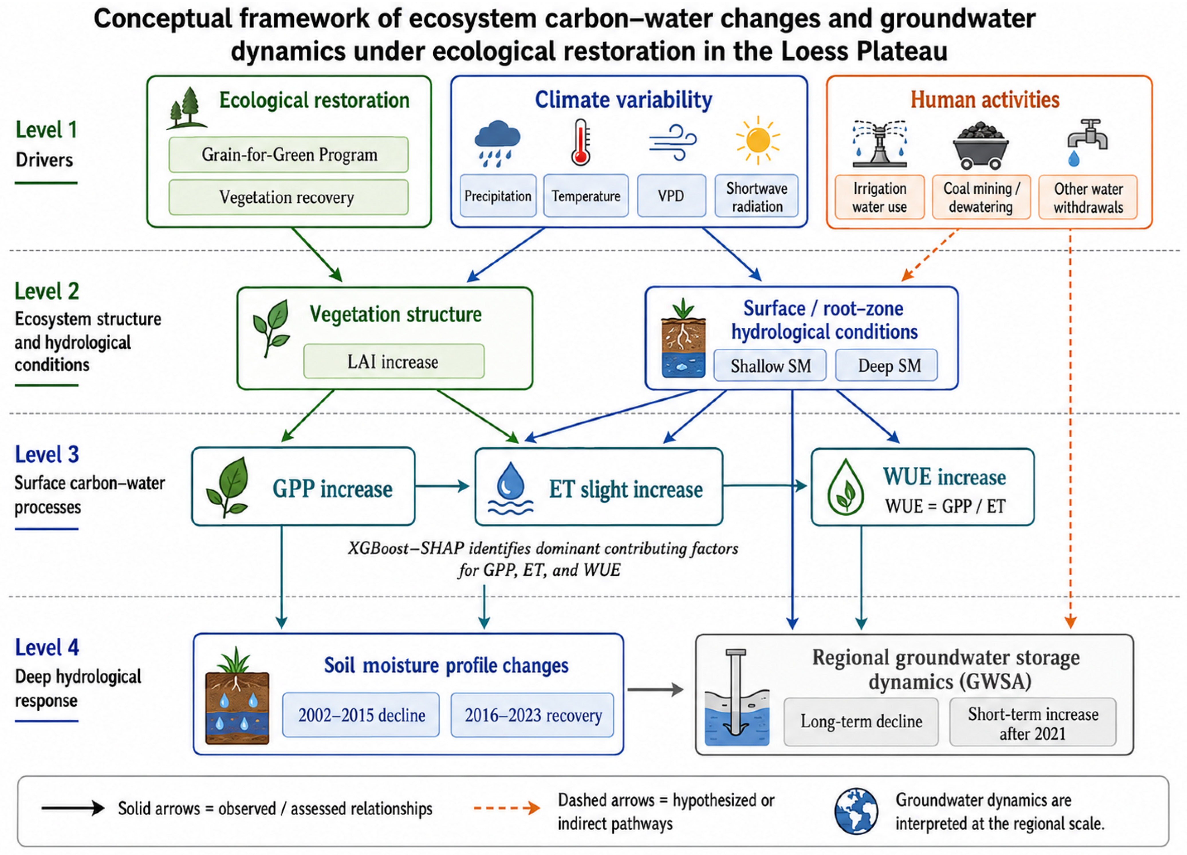
Figure 1. Conceptual framework and analytical pathway of this study. Solid arrows denote observed or modeled surface carbon–water relationships, whereas dashed arrows denote hypothesized recharge pathways or contextual human-activity pathways that were not quantitatively attributed to GWSA. The framework tests whether restoration-associated carbon gain was accompanied by proportional ET and synchronous groundwater recovery.
Remotesensing 18 02822 g001
Figure 2. Interannual variation in precipitation over the Loess Plateau. The red dashed line denotes the fitted long-term trend.
Remotesensing 18 02822 g002
Figure 3. Topography and coal-resource distribution of the Loess Plateau.
Remotesensing 18 02822 g003
Figure 4. Annual GPP and its trend over the Loess Plateau during 2002–2023. (a) Mean annual GPP; (b) spatial trend in GPP; (c) regions showing significant greening or browning; (d) interannual variation in regional mean GPP, where the red dashed line denotes the fitted long-term trend and the red shaded area denotes the corresponding confidence band.
Remotesensing 18 02822 g004
Figure 5. Annual ET and its trend over the Loess Plateau during 2002–2023. (a) Intercomparison of multiple ET products (the black line denotes the multi-product average regional ET series, with a Sen’s slope of 1.40 mm yr−1); (b) mean annual ET; (c) spatial trend in ET; (d) regions showing significant increases or decreases in ET; (e) interannual variation in regional mean ET, where the red dashed line denotes the fitted long-term trend and the red shaded area denotes the corresponding confidence band.
Remotesensing 18 02822 g005
Figure 6. Annual WUE and its trend over the Loess Plateau during 2002–2023. (a) Mean annual WUE; (b) spatial trend in WUE; (c) regions showing significant increases or decreases; (d) interannual variation in regional mean WUE, where the red dashed line denotes the fitted long-term trend and the red shaded area denotes the corresponding confidence band.
Remotesensing 18 02822 g006
Figure 7. Model-based associations of ET, GPP, and WUE based on XGBoost–SHAP. (a) Relative SHAP contribution by ET predictors; (b) SHAP value distribution for ET; (c) relative SHAP contribution by GPP predictors; (d) SHAP value distribution for GPP; (e) relative SHAP contribution by WUE predictors; (f) SHAP value distribution for WUE.
Remotesensing 18 02822 g007
Figure 8. Changes in SM profiles, TWSA, and GWSA. (ad) SM anomalies at 0–10, 10–40, 40–100, and 100–200 cm; (e) annual GWSA derived from CSR and JPL; (f) descriptive GWSA trends during 2002–2020 and 2020–2023, where the red and orange dashed lines denote the fitted trends for the two descriptive subperiods and the corresponding shaded areas denote the confidence bands; (g) spatial trend in TWSA; (h) spatial trend in GWSA.
Remotesensing 18 02822 g008
Figure 9. Human water-use structure (2002–2023) and the spatial pattern of IWU (2004–2019). (a) Water-use structure and trend in Gansu; (b) water-use structure and trend in Inner Mongolia; (c) water-use structure and trend in Shaanxi; (d) water-use structure and trend in Shanxi; (e) spatial distribution of agricultural irrigation in the Loess Plateau. Provincial statistics are presented as regional context and do not exactly represent water use within the LP boundary.
Remotesensing 18 02822 g009
Table 2. Trends in soil-moisture anomalies at different depths during 2002–2015 and 2016–2023.
PeriodDepth (cm)Slope (mm yr−1)p-ValueSignificance
2002–20150–10 cm−0.0680.187 p > 0.05
2002–201510–40−0.0700.634 p > 0.05
2002–201540–100−0.2060.586 p > 0.05
2002–2015100–200−0.3460.385 p > 0.05
2016–20230–100.3190.080 p > 0.05
2016–202310–400.8910.023 p < 0.05
2016–202340–1002.9990.006 p < 0.01
2016–2023100–2002.1900.026 p < 0.05
Table 3. Common-grid quantitative comparison between GWSA-decline and map-defined GPP or ET high-value zones. Strong GWSA decline was defined as a trend 9 mm yr−1; high GPP and high ET were defined as 1200 g C m−2 yr−1 and 550 mm yr−1, respectively. These thresholds follow the spatial-map classification described in Section 2.3.4 and are used only for descriptive overlap analysis.
Spatial ComparisonSpearman’s ρ p ValueOverlap Rate (%)Jaccard Index
GWSA decline vs. GPP−0.0920.16216.90.095
GWSA decline vs. ET−0.0910.16631.00.129
Disclaimer/Publisher’s Note: The statements, opinions and data contained in all publications are solely those of the individual author(s) and contributor(s) and not of MDPI and/or the editor(s). MDPI and/or the editor(s) disclaim responsibility for any injury to people or property resulting from any ideas, methods, instructions or products referred to in the content.