AERO: Arbitrary-Scale Equivariant Resolution Operator for Remote Sensing Image Super-Resolution

Highlights

What are the main findings?

• We introduce the Arbitrary-scale Equivariant Resolution Operator (AERO), a novel continuous representation framework unifying orientation-aware feature modeling, wavelet-domain routing, and relative sub-pixel decoding.
• AERO-Large achieves the best overall performance across all evaluation metrics, reaching a PSNR of 31.02 dB on the WHU-RS19 dataset and reducing rotational variance to 0.0010 dB.

What are the implications of the main findings?

• By integrating orientation-aware feature extraction and wavelet-domain modeling, AERO successfully overcomes the rigid upsampling constraints and spectral biases inherent in traditional super-resolution networks.
• The framework preserves geographic boundaries at arbitrary non-integer scales, making it suitable for practical applications such as interactive GIS analysis and multi-source image fusion.

Abstract

Remote sensing image super-resolution aims to reconstruct high-resolution images from low-resolution observations and is important for image interpretation. Existing fixed-scale methods achieve good performance at predefined integer scales, but their dedicated upsampling modules limit their application to arbitrary-scale scenarios such as interactive GIS and multi-source image fusion. Continuous implicit methods provide scale flexibility but often exhibit spectral bias, resulting in over-smoothed textures and blurred object boundaries. To overcome these limitations, we propose an Arbitrary-scale Equivariant Resolution Operator (AERO) for remote sensing image super-resolution. AERO consists of three components. The Omnidirectional Feature Extractor enhances feature representation under orientation variations. The Wavelet–Arnold Residual Group models low- and high-frequency information in the wavelet domain to preserve textures and geographic boundaries. The Local Implicit Terrain Operator employs relative sub-pixel coordinates for continuous arbitrary-scale reconstruction. Experiments on AID, NWPU-RESISC45, UCMerced, and WHU-RS19 demonstrate that AERO achieves the best performance in the ×4 fixed-scale task. On WHU-RS19, AERO reaches a PSNR of 31.02 dB, exceeding FMSR by 0.64 dB. In rotational robustness experiments, the maximum PSNR fluctuation is reduced from 0.0181 dB to 0.0010 dB. The results show that AERO provides a practical approach for arbitrary-scale remote sensing image super-resolution.

1. Introduction

With the rapid development of satellite remote sensing, unmanned aerial vehicle (UAV) imaging, and Earth observation systems, high-resolution (HR) remote sensing imagery has become an important source of information for land-cover classification, disaster monitoring, urban analysis, agricultural assessment, and ecological observation [1,2,3,4,5]. The spatial resolution of remote sensing images is often constrained by sensor capability, orbital altitude, imaging swath, and data transmission bandwidth [6,7]. As a result, object boundaries may become blurred, fine textures may be lost, and small structures may be degraded, reducing the reliability of downstream interpretation tasks. Single image super-resolution (SISR) reconstructs HR images from low-resolution (LR) observations and provides a cost-effective solution for improving remote sensing image quality without modifying imaging hardware [8,9,10,11,12]. Compared with natural image super-resolution, remote sensing image super-resolution requires not only accurate reconstruction but also arbitrary-scale flexibility, preservation of high-frequency structures, and robustness to orientation variations.

Existing remote sensing image super-resolution methods have mainly followed the fixed-scale reconstruction paradigm. Convolutional neural networks (CNNs) improve local texture reconstruction through hierarchical feature extraction, residual learning, and attention mechanisms. Representative methods, including VDSR, EDSR, and RCAN, achieve good reconstruction performance at standard integer scales [13,14,15,16,17,18,19,20,21,22,23,24]. Transformer-based approaches such as SwinIR and HAT introduce self-attention mechanisms to capture long-range dependencies and improve the reconstruction of complex spatial structures [25,26,27,28,29,30]. More recently, state-space models (SSMs) and Mamba-based methods, including MambaIR and FMSR, have been explored for image restoration and super-resolution because of their ability to model long-range features with relatively low computational cost [31,32,33,34,35,36,37]. While effective at predefined integer scales ($\times 2,\times 3,\times 4$), these discrete paradigms rely on static upsampling modules (e.g., PixelShuffle) that rigidly restrict their outputs. This scale inflexibility limits their utility in interactive geographic information systems (GISs) and dynamic multi-source image fusion [38,39,40,41,42].

Continuous arbitrary-scale super-resolution methods based on implicit neural representations (INRs) have been proposed to overcome the limitations of fixed upsampling. These methods learn the mapping between continuous coordinates and local image features, allowing a single model to generate super-resolved images at both integer and non-integer scales. LIIF demonstrated the feasibility of local implicit decoding for arbitrary-scale super-resolution, while SADN, FunSR, and CiaoSR further improved scale-aware feature interaction and dynamic aggregation [43,44,45,46,47,48,49,50,51,52]. However, coordinate-based implicit decoders often suffer from spectral bias, causing networks to fit low-frequency components more easily than high-frequency details [53,54]. In remote sensing images, high-frequency structures such as building boundaries, road edges, field contours, aircraft wings, and dense human-made objects are important for geographic interpretation. Excessive smoothing of these structures may lead to boundary degradation, local topological distortion, and reduced reliability in downstream applications. Generative super-resolution methods, including GAN-based and diffusion-based approaches, can produce sharper visual textures [55,56,57,58]. However, they may also introduce non-existent buildings, roads, or textures, which limits their applicability in remote sensing tasks that require spatial consistency and structural reliability [11].

To preserve structural details, frequency-domain priors have been introduced into super-resolution networks. The discrete wavelet transform (DWT) decomposes image features into low-frequency approximation components and high-frequency detail components, providing an explicit representation of edges, textures, and directional structures [59,60,61,62]. Wavelet-domain modeling is not limited to continuous super-resolution. It serves as a general frequency-domain prior that can improve boundary preservation in discrete models and provide high-frequency constraints for continuous implicit decoders. Existing wavelet-based methods still have two limitations. First, most methods employ static activation functions, such as ReLU or GELU, which cannot adapt to the spatially varying frequency distributions in remote sensing images. Second, satellite and aerial images are commonly acquired from a top-down perspective, where buildings, runways, ships, and roads may appear at different orientations. Existing models generally lack explicit orientation-aware feature modeling, which can result in unstable reconstruction under orientation changes [63]. Current methods mainly address fixed-scale reconstruction, arbitrary-scale decoding, high-frequency preservation, or orientation robustness separately, while frameworks that consider these requirements simultaneously remain limited.

This paper proposes an Arbitrary-scale Equivariant Resolution Operator (AERO) for remote sensing image super-resolution. AERO integrates orientation-aware feature extraction, frequency-domain modeling, and continuous implicit decoding within a unified framework. The Omnidirectional Feature Extractor (OFE) processes multiple orthogonal rotated views and aligns the extracted features to the original coordinate system to improve feature representation under orientation variations. The Wavelet–Arnold Residual Group (WARG) combines Haar wavelet decomposition with a learnable KAN-inspired dynamic activation function to model geographic frequency distributions and preserve high-frequency structures. The Local Implicit Terrain Operator (LITO) maps fused features to continuous HR coordinate space using relative sub-pixel coordinates and continuous cell size information, improving boundary preservation during arbitrary-scale decoding.

The main contributions of this paper are summarized as follows:

• We propose AERO, an arbitrary-scale super-resolution framework for remote sensing imagery. The proposed framework integrates fixed-scale reconstruction and continuous arbitrary-scale decoding within a single network, enabling both integer-scale and arbitrary-scale reconstruction.
• We design an Omnidirectional Feature Extractor (OFE) for orientation-aware feature representation. By extracting and aligning features from multiple orthogonal rotated views, OFE improves reconstruction stability under orientation variations in remote sensing scenes.
• We develop a Wavelet–Arnold Residual Group (WARG). The proposed module combines Haar wavelet-domain modeling and a learnable dynamic frequency activation function to preserve high-frequency structures, including building edges, road contours, and field boundaries.
• We introduce a Local Implicit Terrain Operator (LITO) for arbitrary-scale continuous decoding. By incorporating relative sub-pixel coordinates and continuous cell size information, LITO reduces boundary blurring and local topological distortion at non-integer scales.

The remainder of this paper is organized as follows. Section 2 reviews related work on remote sensing image super-resolution, including discrete feature-learning models, continuous implicit representation methods, generative super-resolution, and frequency-domain priors. Section 3 presents the proposed AERO framework and its components. Section 4 describes the experimental settings and reports quantitative, qualitative, and ablation results. Section 5 discusses the advantages, limitations, and potential applications of the proposed method. Section 6 concludes the paper and outlines future research directions.

2. Related Work

2.1. Orientation-Aware Feature Extraction in Remote Sensing

Single Image Super-Resolution (SISR) addresses the trade-off between spatial resolution and swath width in satellite and aerial optical sensors [10]. Compared with terrestrial images, remote sensing imagery exhibits large intra-class scale variations, dense high-frequency textures, and arbitrary target orientations. As a result, directly applying general computer vision SR models to remote sensing images may produce blurred boundaries and rotational artifacts [64,65]. These characteristics have motivated the development of remote sensing SR methods and benchmark datasets, including UCMerced [66] and WHU-RS19 [67]. Larger datasets such as the Aerial Image Dataset (AID) [68] and NWPU-RESISC45 [69], containing 10,000 and 31,500 images, respectively, provide sufficient scene diversity for training modern super-resolution networks.

Remote sensing applications generally involve two super-resolution paradigms. The first is discrete (fixed-scale) SR, which reconstructs images at predefined resolution scales and is commonly used in standardized satellite imaging tasks [39]. The second is continuous (arbitrary-scale) SR, which supports interactive Geographic Information Systems (GISs) and multi-sensor data fusion by enabling image reconstruction at arbitrary scaling factors [42].

Convolutional Neural Networks (CNNs) established the foundation of discrete super-resolution through hierarchical feature extraction. VDSR demonstrated that deep residual networks combined with gradient clipping can improve training convergence [15], while EDSR increased network capacity and reduced memory consumption by removing batch normalization layers [16]. RCAN further increased network depth by introducing residual-in-residual structures and channel attention mechanisms to emphasize informative features [17]. Owing to their computational efficiency, CNN-based methods have been widely adopted in remote sensing image super-resolution [24]. However, their receptive fields are inherently constrained by local convolution kernels, which limits the modeling of long-range spatial dependencies, such as extended road networks [70]. In addition, conventional CNN-based methods commonly employ fixed upsampling modules, such as PixelShuffle, resulting in outputs restricted to predefined integer scales.

Vision Transformers (ViTs) were introduced to super-resolution to model long-range dependencies through self-attention mechanisms [26]. SwinIR adopted window-based self-attention to reduce computational cost [28,71], while HAT introduced overlapping cross-attention between neighboring windows to improve feature interaction [27]. Although these methods improve global feature modeling, the quadratic computational complexity of self-attention remains a limitation. For large remote sensing images with high spatial resolution and dense textures, the associated memory consumption can restrict model scalability and practical deployment [30].

State-Space Models (SSMs) have recently been explored as an alternative to Transformer architectures because they provide long-range feature modeling with linear computational complexity [35]. MambaIR introduced selective scanning mechanisms for image restoration tasks [34], and FMSR further adapted this framework for remote sensing image super-resolution by combining spatial and frequency-domain information [33,72]. Nevertheless, studies such as that on MambaOut have pointed out that SSMs are primarily designed for one-dimensional sequence modeling [36]. The conversion of two-dimensional remote sensing images into one-dimensional sequences may weaken local spatial relationships and make orientation variations more difficult to model. In addition, the recurrent hidden-state computation of SSMs limits full parallel execution, which may reduce computational efficiency in continuous-scale reconstruction tasks. In summary, standard discrete feature-learning models rely on rigid spatial grids and 1D scanning mechanisms that fail to natively capture the arbitrary orientation of top-down satellite imagery. Our proposed Omnidirectional Feature Extractor (OFE) directly addresses this gap by explicitly enforcing rotational equivariance at the shallow feature-extraction stage.

2.2. Continuous Decoding and Local Implicit Representations

Implicit Neural Representations (INRs) [43] model continuous image signals by mapping spatial coordinates and local features to RGB values using Multi-Layer Perceptrons (MLPs). LIIF demonstrated that this framework enables arbitrary-scale image reconstruction using a single model [45]. This approach has subsequently been applied to remote sensing imagery. FunSR introduced context-aware interactions in the implicit space to better represent geographic scene variations [47], while SADN incorporated scale-aware dynamic convolutions to adjust network parameters according to the target scale and reduce performance degradation at unseen magnification factors [46,73].

Continuous super-resolution methods have also incorporated dynamic feature aggregation mechanisms [50]. CiaoSR introduced an attention-in-attention mechanism to estimate dynamic ensemble weights and combine self-attention with arbitrary-scale decoding [48]. Despite these developments, coordinate-based MLP decoders remain affected by spectral bias [53]. Such models tend to represent low-frequency components more easily than high-frequency details [54]. In remote sensing images, high-frequency structures such as building boundaries and field edges are important for geographic interpretation, and the loss of these details may lead to boundary blurring and structural degradation [42]. To overcome the spectral bias and boundary blurring inherent in these spatially blind MLPs, our proposed Local Implicit Terrain Operator (LITO) injects localized relative sub-pixel coordinates to act as a dynamic geometric anchor during continuous decoding.

2.3. Dynamic Frequency-Domain and Wavelet Priors

Generative super-resolution methods have been developed to improve the perceptual quality of reconstructed images. ESRGAN introduced Residual-in-Residual Dense Blocks (RRDBs) to enhance texture reconstruction [55], while Real-ESRGAN incorporated high-order degradation modeling for real-world image restoration [56,74]. Diffusion-based approaches have also been applied to super-resolution. SR3 employed conditional iterative refinement [58], and ResShift improved sampling efficiency by performing diffusion in the residual space [57]. Although these methods can generate visually realistic textures, they may also introduce artificial structures that are not present in the original scene. In remote sensing applications, the generation of non-existent buildings or modified geographic structures can reduce the reliability of reconstructed images [11].

The Discrete Wavelet Transform (DWT) [59] has been introduced to preserve structural information by separating low-frequency and high-frequency components [62]. MWCNN [60] incorporated wavelet representations into discrete super-resolution networks to improve boundary preservation, while LIWT [61] integrated wavelet priors into implicit decoders to alleviate spectral bias and reduce over-smoothing. Within the specific domain of remote sensing, wavelet priors have been successfully leveraged to preserve complex geographic textures. For example, recent studies have utilized wavelet-guided feature refinement networks to explicitly recover high-frequency satellite edge data that standard convolutions discard [75,76]. Nevertheless, existing wavelet-based methods generally employ static activation functions, such as ReLU, which may not adapt effectively to the frequency variations in remote sensing images. In addition, these methods typically do not explicitly consider orientation variations in satellite imagery. Because static activations fail to dynamically route the extreme variance of geographic high-frequency distributions, our Wavelet–Arnold Residual Group (WARG) introduces a parameterized KAN-inspired activation within the wavelet domain to adaptively preserve critical boundaries.

3. Method

3.1. Overall Architecture of AERO

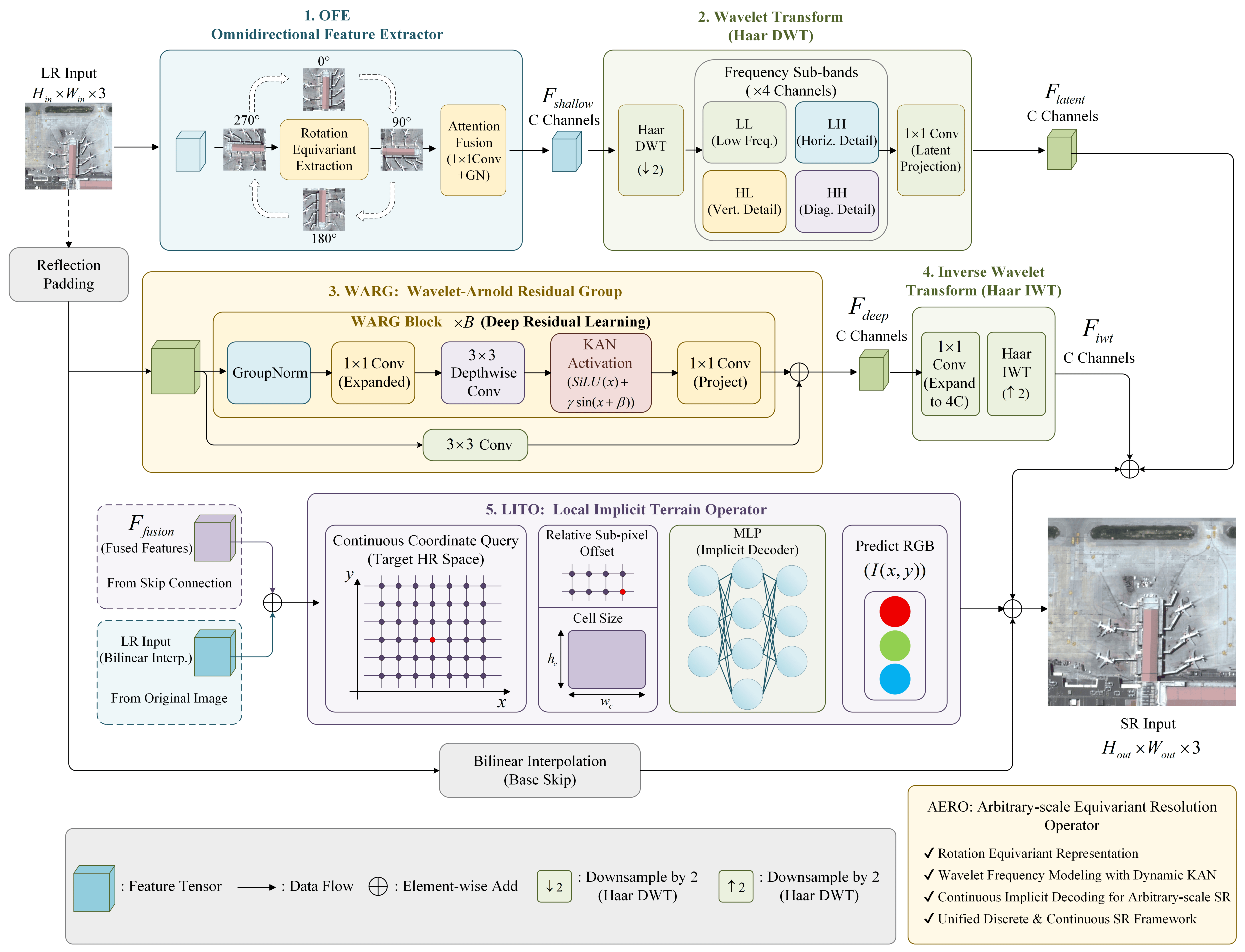
As shown in Figure 1, AERO is an end-to-end framework that combines frequency-domain feature modeling with implicit neural representations for both discrete and arbitrary-scale super-resolution.

Given a low-resolution (LR) remote sensing image $\mathbf{I}LR\in {\mathbb{R}}^{3\times H\times W}$, the network first extracts shallow features using the OFE, which is designed to improve feature representation under orientation variations. The shallow feature extraction can be denoted as:

$${\mathbf{F}}_{shallow}=\mathrm{OFE}\left({\mathbf{I}}_{LR}\right),{\mathbf{F}}_{shallow}\in {\mathbb{R}}^{C\times H\times W}$$

(1)

To separate high-frequency structures from low-frequency components while reducing computational cost, ${\mathbf{F}}_{shallow}$ is transformed into the wavelet domain using the DWT with Haar wavelets. This operation reduces the spatial resolution by a factor of 2 and produces four frequency sub-bands (LL, LH, HL, HH). A $1\times 1$ convolution is then applied to project the features into the latent space:

$${\mathbf{F}}_{latent}={\mathrm{Conv}}_{1\times 1}\left(\mathrm{DWT}\left({\mathbf{F}}_{shallow}\right)\right),{\mathbf{F}}_{latent}\in {\mathbb{R}}^{C\times {\displaystyle \frac{H}{2}}\times {\displaystyle \frac{W}{2}}}$$

(2)

The latent features are subsequently processed by a series of N WARG. The deep features are modeled using a global residual connection:

$${\mathbf{F}}_{deep}={\mathbf{F}}_{latent}+{\mathrm{Conv}}_{3\times 3}\left({\mathrm{WARG}}_N(\cdots {\mathrm{WARG}}_1\left({\mathbf{F}}_{latent}\right)\cdots )\right)$$

(3)

After deep feature extraction, a $1\times 1$ convolution expands the channel dimension to $4C$, and the Inverse Wavelet Transform (IWT) restores the spatial resolution to $H\times W$. The reconstructed features are fused with the shallow features through a long skip connection:

$${\mathbf{F}}_{fusion}={\mathbf{F}}_{shallow}+\mathrm{IWT}\left({\mathrm{Conv}}_{1\times 1}\left({\mathbf{F}}_{deep}\right)\right)$$

(4)

Finally, the fused features $\mathbf{F}fusion$ are fed into the LITO for arbitrary-scale reconstruction. LITO predicts the RGB values of the target high-resolution (HR) image by querying continuous spatial coordinates. A global bilinear interpolation branch is added to preserve low-frequency information:

$${\mathbf{I}}_{SR}=\mathrm{LITO}({\mathbf{F}}_{fusion},H_{out},W_{out})+f_{bilinear}({\mathbf{I}}_{LR},H_{out},W_{out})$$

(5)

where $H_{out}$ and $W_{out}$ correspond to the target arbitrary spatial dimensions dictated by the continuous scale factor, s.

3.2. Omnidirectional Feature Extractor (OFE)

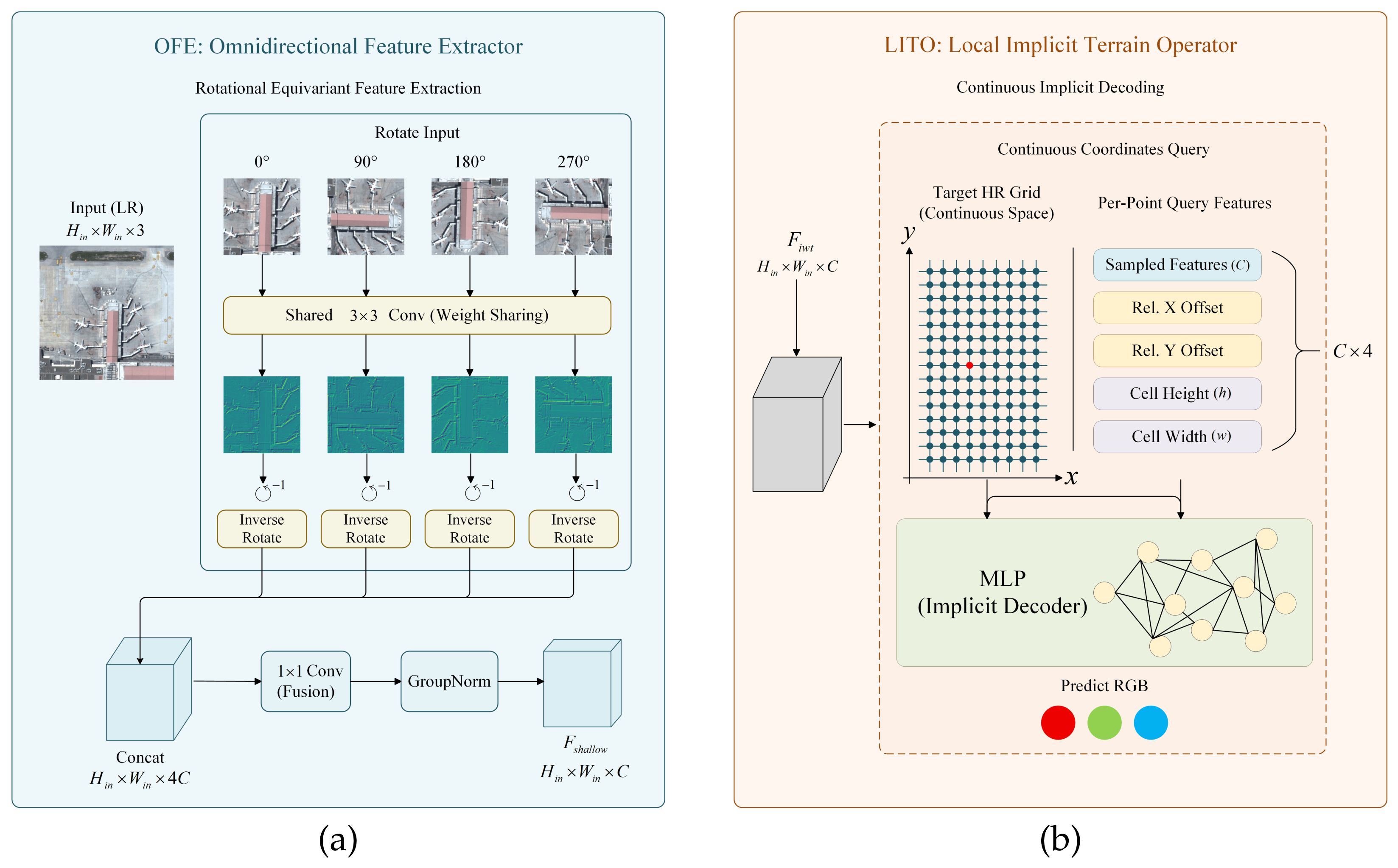
Unlike natural images which predominantly feature fixed, gravity-aligned orientations, remote sensing imagery is captured in a top-down manner, resulting in arbitrary 360-degree object orientations (e.g., runways, ships, and buildings). Standard convolutional layers struggle to generalize across these rotations due to their rigid grid structures. To mitigate this, we design the Omnidirectional Feature Extractor (OFE), as detailed in Figure 2a, which approximates discrete rotational invariance at the shallow feature level. While canonical group-equivariant networks such as E(2)-CNN provide rigorous continuous rotational equivariance, they incur substantial computational overheads that scale poorly with massive high-resolution remote sensing imagery. In contrast, the OFE provides a highly efficient, practical trade-off by performing explicit multi-view feature fusion.

Given the input ${\mathbf{I}}_{LR}$, the OFE first generates four distinct mathematical rotations: $\theta \in \{0°,90°,180°,270°\}$. A shared $3\times 3$ convolutional kernel is applied simultaneously across all four rotational views, ensuring the weights learn rotation-agnostic geospatial patterns. Let ${\mathcal{R}}^{\theta }(·)$ denote the spatial rotation operator. The feature extraction for each angle is formulated as:

$${\mathbf{f}}_{\theta }={\mathrm{Conv}}_{3\times 3}\left({\mathcal{R}}^{\theta }\left({\mathbf{I}}_{LR}\right)\right)$$

(6)

To spatially align the extracted features back to the original coordinate system, an inverse rotation ${\mathcal{R}}^{-\theta }(·)$ is applied. The four aligned feature maps are then concatenated along the channel dimension and collapsed back to the target feature dimension C via an attention-driven $1\times 1$ convolution, followed by Group Normalization (GN):

$${\mathbf{F}}_{shallow}=\mathrm{GN}\left({\mathrm{Conv}}_{1\times 1}\left({\mathrm{Concat}}_{\theta }\left({\mathcal{R}}^{-\theta }\left({\mathbf{f}}_{\theta }\right)\right)\right)\right)$$

(7)

By explicitly processing orthogonal perspectives and fusing them, the OFE prevents the network from memorizing orientation biases within the training dataset, yielding highly robust representations for complex terrains.

3.3. Wavelet–Arnold Residual Group (WARG)

Continuous decoders often suffer from spectral bias, heavily suppressing high-frequency edges. To ensure critical boundary data is preserved, AERO processes features in the wavelet domain. However, traditional networks utilize static, rigid activation functions (e.g., ReLU or GELU) that are ill-equipped to handle the extreme variance of geographic high-frequency distributions. To solve this, we propose the Wavelet–Arnold Residual Group (WARG), leveraging a continuous, parameterized basis function inspired by the dynamic non-linear fitting concept of Kolmogorov–Arnold Networks (KANs).

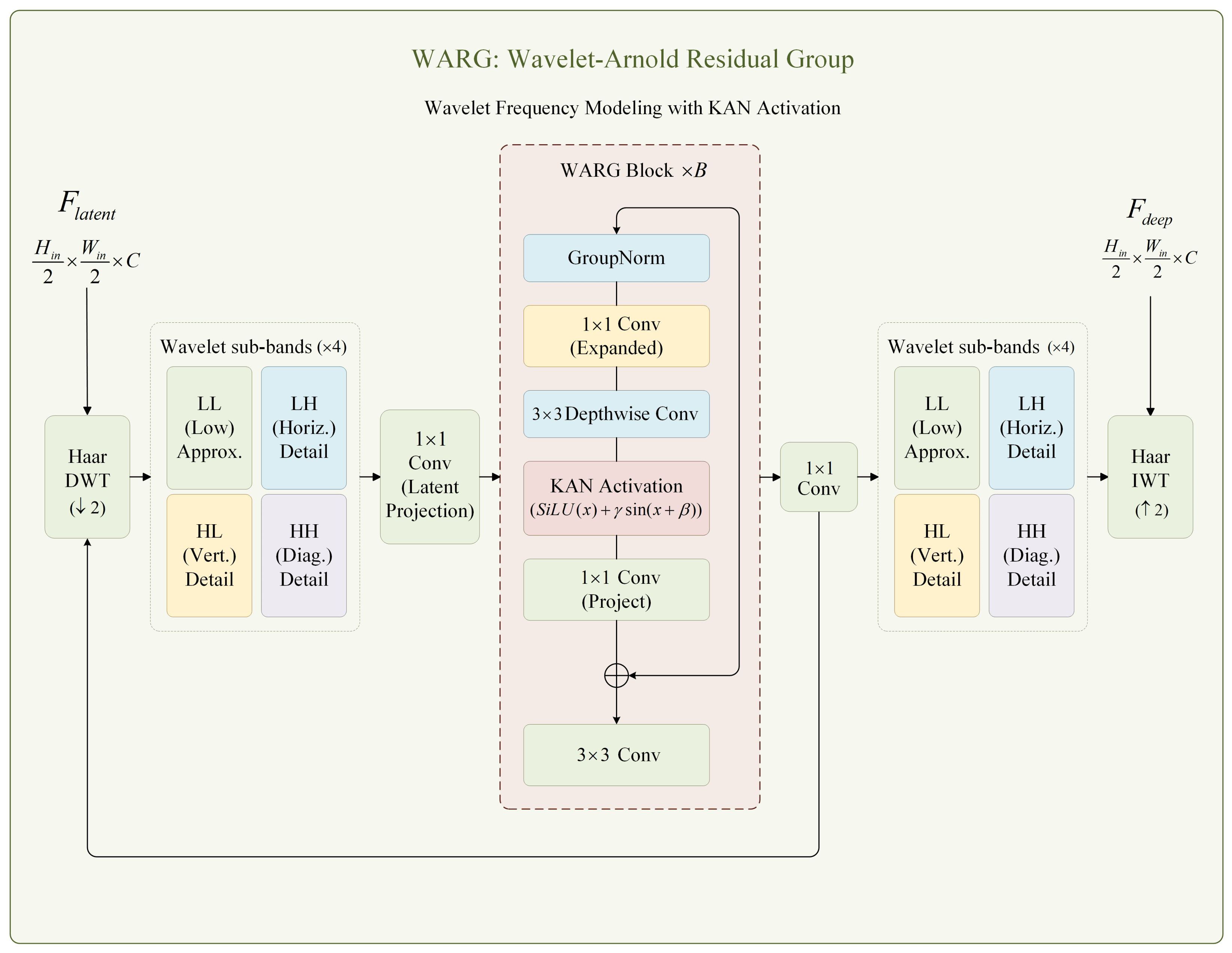
As shown in Figure 3, each WARG Block utilizes an inverted bottleneck architecture. The input feature $\mathbf{x}$ is first normalized via GroupNorm, expanded in the channel dimension via a $1\times 1$ point-wise convolution, and spatially correlated using a $3\times 3$ depthwise convolution. The core innovation lies in the subsequent WKAN Activation. While vanilla KAN utilizes explicit piecewise B-spline grids to replace fixed activation functions, applying exact spatial splines across high-resolution 2D remote sensing feature maps introduces prohibitive computational and memory overheads. Therefore, WKAN explicitly borrows the core design logic of KAN—employing learnable, dynamic basis functions—but adapts it for efficient spatial processing. Instead of utilizing traditional splines, WKAN functions as a lightweight alternative that couples a base approximation (SiLU) with a learnable, high-frequency Sine wave detail catcher:

$$\mathrm{WKAN}\left(\mathbf{z}\right)=\mathbf{z}·\sigma \left(\mathbf{z}\right)+\mathit{\gamma }\odot \sin (\mathbf{z}+\mathit{\beta })$$

(8)

where $\mathbf{z}$ represents the depthwise feature maps, $\sigma (·)$ is the Sigmoid function (forming the SiLU operation), and $\mathit{\gamma },\mathit{\beta }\in {\mathbb{R}}^C$ are learnable scaling and phase-shift parameters, broadcast across the spatial dimensions.

From a Fourier-domain perspective, let $\mathcal{F}(·)$ denote the Fourier transform. The static SiLU approximation $\mathbf{z}·\sigma \left(\mathbf{z}\right)$ primarily acts as a low-pass filter, preserving the DC component and low-frequency terrain approximations. The addition of the parameterized sine wave $\mathit{\gamma }\odot \sin (\mathbf{z}+\mathit{\beta })$ introduces a controlled, high-frequency modulation. In the frequency domain, this is equivalent to convolving the feature spectrum with shifted Dirac delta functions, explicitly pulling high-frequency edge information back into the active passband without requiring deeper convolutional layers.

By parameterizing the amplitude ($\mathit{\gamma }$) and phase ($\mathit{\beta }$) of the sine wave, the network dynamically adapts its frequency filtering behavior based on the specific terrain semantics (e.g., applying aggressive high-frequency routing for dense urban structures, while suppressing noise in homogeneous water bodies). Following activation, the features are projected back to the original dimension via a $1\times 1$ convolution and added to the block input via a residual connection.

3.4. Local Implicit Terrain Operator (LITO)

Standard super-resolution networks rely on discrete upsampling modules (e.g., PixelShuffle), permanently restricting them to integer scale factors ($\times 2,\times 3,\times 4$). To overcome this, AERO concludes with the LITO, a continuous neural decoder designed to query the deep fused features, ${\mathbf{F}}_{fusion}$, using arbitrary spatial coordinates, as illustrated in Figure 2b.

However, traditional implicit decoders (such as LIIF) frequently suffer from spatial blindness—yielding blurred topological boundaries—if they are not provided with localized sub-pixel geometry. To mathematically guarantee sharp boundaries at any arbitrary scale, LITO explicitly feeds relative sub-pixel coordinates into the decoding Multi-Layer Perceptron (MLP).

Given a target continuous HR grid of size $H_{out}\times W_{out}$, we generate a continuous coordinate domain scaled to $[-1,1]$. For every HR coordinate query, we project it back onto the continuous LR boundaries $[0,W_{in}]$ and $[0,H_{in}]$. To grant the MLP dynamic spatial filtering capabilities, we calculate the exact fractional offset $(\Delta x,\Delta y)$ of the HR coordinate relative to the center of its corresponding LR cell:

$$\Delta x=x_{lr}-\lfloor x_{lr}\rfloor -0.5,\Delta y=y_{lr}-\lfloor y_{lr}\rfloor -0.5$$

(9)

Concurrently, the bilinearly interpolated feature vector ${\mathbf{f}}_{sampled}\in {\mathbb{R}}^C$ is sampled from ${\mathbf{F}}_{fusion}$ at the corresponding projected coordinates. To inform the MLP of the exact requested scale, continuous cell dimensions are defined as $h_c=2.0/H_{out}$ and $w_c=2.0/W_{out}$.

The final input vector $\mathbf{v}$ presented to the implicit MLP comprises the sampled features, the relative sub-pixel coordinates, and the continuous cell size:

$$\mathbf{v}=\left[{\mathbf{f}}_{sampled},\Delta x,\Delta y,h_c,w_c\right]\in {\mathbb{R}}^{C+4}$$

(10)

By querying the deep implicit decoder $f_{MLP}$ with $\mathbf{v}$, LITO predicts the exact RGB scalar values for the continuous coordinate:

$${\mathbf{I}}_{LITO}(x,y)=f_{MLP}\left(\mathbf{v}\right)$$

(11)

The inclusion of explicit sub-pixel offsets ($\Delta x,\Delta y$) acts as a geometric anchor, granting LITO the spatial awareness required to draw razor-sharp, sub-meter remote sensing boundaries that traditional coordinate-based networks blur.

4. Experiments

To rigorously validate AERO across the diverse operational requirements of remote sensing, our evaluation is explicitly bifurcated into two testing paradigms: discrete (fixed-integer) and continuous (arbitrary-scale) super-resolution. This separation is methodologically necessary because continuous implicit models—while providing the critical flexibility of infinite, non-integer zoom—typically sacrifice peak mathematical fidelity on fixed grids when compared to dedicated discrete state-of-the-art (SoTA) architectures. By evaluating AERO within both domains independently, we demonstrate its unique capacity to deliver the topological flexibility of continuous models without conceding the peak mathematical performance demanded by discrete standards.

4.1. Datasets and Metrics

To comprehensively evaluate the generalization and structural fidelity of the proposed AERO architecture, we conduct extensive experiments across four widely adopted, large-scale remote sensing benchmarks:

• AID [68]: A massive-scale aerial image dataset comprising 10,000 images distributed across 30 diverse scene categories, with a native spatial resolution of $600\times 600$ pixels.
• NWPU-RESISC45 [69]: One of the richest remote sensing benchmarks, containing 31,500 images across 45 classes at a resolution of $256\times 256$ pixels, featuring extreme intra-class variation.
• UCMerced LandUse [66]: A foundational dataset containing 2100 images across 21 land-use classes, with a spatial resolution of $256\times 256$ pixels.
• WHU-RS19 [67]: A high-resolution satellite dataset comprising 1005 images across 19 classes, featuring a native resolution of $600\times 600$ pixels.

For all datasets, we adhere to a strict 8:2 train–test split, utilizing $80\%$ of the images for training and reserving the remaining $20\%$ for validation and evaluation. During evaluation, to reflect real-world operational scenarios, the networks are tested on the full, uncropped original images rather than small, isolated patches.

To quantitatively assess reconstruction quality, we employ three standard evaluation metrics. For mathematical distortion and pixel-wise fidelity, we use Peak Signal-to-Noise Ratio (PSNR) and the Structural Similarity Index Measure (SSIM) [77]. Both PSNR and SSIM are evaluated on the standard $[0,1]$ RGB tensor range to capture full color-space reconstruction accuracy. To evaluate human-aligned visual perception and structural authenticity, we utilize the Learned Perceptual Image Patch Similarity (LPIPS) [78] metric, utilizing the pre-trained AlexNet backbone. Higher PSNR and SSIM values indicate superior mathematical fidelity, while a lower LPIPS score denotes better perceptual quality and fewer structural hallucinations.

4.2. Implementation Details

The proposed AERO architecture and all continuous/discrete variants were implemented using the PyTorch 2.10 framework. Training was conducted in a fully parallelized environment using Distributed Data Parallel (DDP) across an infrastructure equipped with four NVIDIA Tesla V100 (16 GB SXM2) GPUs, an Intel Xeon E5-2630 v4 CPU (@ 2.20 GHz), and 32 GB of DDR4 RAM.

During the training phase, the high-resolution (HR) ground-truth images were randomly cropped into $256\times 256$ patches, and the corresponding low-resolution (LR) inputs were generated via mathematically exact bicubic downsampling. We employed a batch size of 16 per GPU, resulting in an effective global batch size of 64. The models were trained from scratch for a total of 50,000 optimization steps. To guarantee a strictly fair and objective horizontal evaluation, all compared baseline architectures across both discrete and continuous paradigms—including traditional CNNs, Vision Transformers, State-Space Models, and implicit neural networks—were fully reimplemented and trained from scratch utilizing this exact unified experimental configuration (identical dataset splits, degradation pipelines, optimizers, and learning rate schedules).

To optimize the network, we utilized the AdamW optimizer [79], which pairs exceptionally well with Implicit Neural Operators (LITOs) and KAN-inspired activations, setting the initial learning rate to $2\times {10}^{-4}$ and weight decay to $1\times {10}^{-4}$. The learning rate was dynamically decayed using a Cosine Annealing scheduler ($T_{max}=100$) down to a minimum threshold of ${\eta }_{min}=1\times {10}^{-6}$. The network was optimized using the $L_1$ absolute error loss to prevent the over-smoothing typically induced by $L_2$ penalties. Furthermore, to guarantee stability when propagating gradients through the continuous frequency basis functions (WKAN) and coordinate grids, strict gradient clipping was enforced with a maximum norm of $1.0$.

To demonstrate structural scalability, we instantiated three variants of the proposed architecture: AERO-Tiny ($C=96$, 4 WARG groups, 4 blocks per group), AERO-Base ($C=128$, 6 groups, 6 blocks), and AERO-Large ($C=192$, 8 groups, 8 blocks). Unless otherwise specified in the ablation studies, the AERO-Large variant serves as baseline for validation.

4.3. Comparisons with State-of-the-Art

To comprehensively evaluate AERO, we compare our architecture against a broad spectrum of state-of-the-art (SoTA) models. For a rigorous assessment, the evaluation is divided into discrete (fixed-scale) benchmarks and continuous (arbitrary-scale) benchmarks.

4.3.1. Discrete Super-Resolution Performance

In the discrete SR paradigm, we compare AERO against 13 leading architectures across various methodologies, including CNN-based models (SRCNN, VDSR, EDSR, RCAN, HAN, SAN, NLSA), Vision Transformers (SwinIR, TransENet, HAT, SRFormer), and recent State-Space Models (MambaIR, FMSR). All models are evaluated at a challenging $\times 4$ upsampling scale across the AID, UCMerced, NWPU-RESISC45, and WHU-RS19 datasets. The quantitative results are presented in

Table 1. Quantitative comparison of discrete SR models at scale factor $\times 4$. The best, second-best, and third-best results are highlighted in bold, underline, and double underline, respectively.

Method	AID $\times 4$				UCMerced $\times 4$				NWPU-RESISC45 $\times 4$				WHU-RS19 $\times 4$
	PSNR	SSIM	LPIPS		PSNR	SSIM	LPIPS		PSNR	SSIM	LPIPS		PSNR	SSIM	LPIPS
Bicubic	27.56	0.7120	0.4909		25.28	0.6621	0.4860		26.33	0.6725	0.5261		28.04	0.7270	0.4549
SRCNN [14]	28.67	0.7571	0.3376		26.79	0.7067	0.3877		27.31	0.7102	0.3982		28.92	0.7688	0.3472
VDSR [15]	29.01	0.7746	0.3284		27.01	0.7112	0.3590		27.39	0.7180	0.3497		29.76	0.7761	0.3012
EDSR [16]	29.31	0.7865	0.3109		27.24	0.7304	0.3029		27.48	0.7298	0.3323		29.82	0.7834	0.2946
RCAN [17]	29.39	0.7906	0.3228		27.26	0.7398	0.3108		27.52	0.7332	0.3279		29.88	0.7924	0.2844
HAN [21]	29.39	0.7905	0.3191		27.30	0.7426	0.3098		27.54	0.7380	0.3210		29.91	0.7965	0.2821
SAN [20]	29.41	0.7912	0.3238		27.28	0.7365	0.3127		27.60	0.7436	0.3099		29.95	0.7978	0.2783
NLSA [22]	29.44	0.7910	0.3134		27.31	0.7487	0.3150		27.63	0.7503	0.3112		29.96	0.7982	0.2778
SwinIR [28]	29.45	0.7901	0.3201		27.32	0.7520	0.3009		27.64	0.7522	0.3013		29.98	0.7993	0.2756
TransENet [25]	29.47	0.7890	0.3134		27.34	0.7496	0.2982		27.70	0.7569	0.2945		30.06	0.7994	0.2751
HAT [27]	29.48	0.7908	0.3110		27.34	0.7533	0.2978		27.68	0.7568	0.2862		30.10	0.8003	0.2742
MambaIR [34]	29.51	0.7922	0.3122		27.38	0.7626	0.2903		27.70	0.7601	0.2928		30.14	0.8011	0.2731
SRFormer [29]	29.51	0.7928	0.3099		27.42	0.7629	0.2826		27.73	0.7624	0.2910		30.22	0.8028	0.2723
FMSR [33]	29.59	0.7942	0.3065		27.36	0.7610	0.2821		27.81	0.7623	0.2889		30.38	0.8029	0.2708
AERO-Tiny	29.55±0.015	0.7962±0.0004	0.3178±0.0012		27.21±0.018	0.7438±0.0005	0.3031±0.0013		27.72±0.014	0.7610±0.0004	0.2901±0.0011		30.47±0.016	0.8038±0.0005	0.2710±0.0010
AERO-Base	29.63±0.014	0.7989±0.0003	0.3059±0.0010		27.35±0.016	0.7522±0.0004	0.2926±0.0012		27.92±0.013	0.7689±0.0006	0.2887±0.0008		30.66±0.012	0.8096±0.0003	0.2687±0.0008
AERO-Large	29.91±0.012	0.8086±0.0003	0.3039±0.0008		27.78±0.015	0.7812±0.0003	0.2719±0.0011		28.10±0.011	0.7723±0.0003	0.2808±0.0009		31.02±0.014	0.8165±0.0005	0.2654±0.0007

.

As observed in Table 1, the AERO-Large variant establishes a new state of the art across all datasets. To verify statistical significance and rule out performance fluctuations induced by random training initialization, we conducted five independent training trials for the proposed AERO variants, reporting the mean and standard deviation. On the WHU-RS19 dataset, AERO-Large yielded a highly stable PSNR of $31.02\pm 0.014$ dB and an SSIM of $0.8165\pm 0.0005$. These exceptionally low standard deviations confirm that the performance margins over baseline architectures are statistically robust. Notably, on the WHU-RS19 dataset, AERO-Large achieves a mean PSNR of 31.02 dB, surpassing the leading Mamba-based FMSR by a remarkable margin of +0.64 dB. Furthermore, even the highly parameter-efficient AERO-Base and AERO-Tiny variants consistently outperform heavy Transformer networks like HAT and SwinIR. This proves that explicitly addressing rotational variance via the OFE and routing high-frequency data via the WARG blocks yields vastly superior geographic reconstructions compared to standard self-attention mechanisms.

To further investigate AERO’s adaptability across diverse semantic landscapes, we provide a detailed, category-by-category breakdown of performance on the 30 classes of the AID dataset in

Table 2. Detailed PSNR (dB) and SSIM comparison across all 30 scene categories of the AID dataset at scale factor $\times 4$. The best, second-best, and third-best results are highlighted in bold, underline, and double underline.

Category	Bicubic			EDSR			RCAN			SwinIR			HAT			MambaIR			SRFormer			FMSR			AERO-Tiny			AERO-Base			AERO-Large
	PSNR	SSIM		PSNR	SSIM		PSNR	SSIM		PSNR	SSIM		PSNR	SSIM		PSNR	SSIM		PSNR	SSIM		PSNR	SSIM		PSNR	SSIM		PSNR	SSIM		PSNR	SSIM
Airport	27.71	0.7489		29.48	0.8169		29.56	0.8210		29.62	0.8205		29.65	0.8212		29.68	0.8226		29.68	0.8232		29.84	0.8255		29.72	0.8266		29.81	0.8292		30.11	0.8393
BareLand	36.26	0.8646		37.87	0.9074		37.95	0.9115		38.01	0.9110		38.04	0.9117		38.07	0.9131		38.07	0.9137		37.72	0.9005		38.11	0.9171		38.16	0.9178		38.32	0.9201
BaseballF.	28.63	0.7852		30.70	0.8526		30.78	0.8567		30.84	0.8562		30.87	0.8569		30.90	0.8583		30.90	0.8589		31.13	0.8592		30.94	0.8623		31.05	0.8646		31.41	0.8726
Beach	32.01	0.7998		33.59	0.8448		33.67	0.8489		33.73	0.8484		33.76	0.8491		33.79	0.8505		33.79	0.8511		33.54	0.8424		33.83	0.8545		33.89	0.8555		34.07	0.8589
Bridge	28.53	0.7750		30.46	0.8359		30.54	0.8400		30.60	0.8395		30.63	0.8402		30.66	0.8416		30.66	0.8422		30.96	0.8419		30.70	0.8456		30.80	0.8476		31.17	0.8553
Center	25.30	0.6984		27.43	0.7817		27.51	0.7858		27.57	0.7853		27.60	0.7860		27.63	0.7874		27.63	0.7880		28.06	0.8056		27.67	0.7914		27.78	0.7955		28.19	0.8098
Church	22.40	0.5797		24.28	0.6908		24.36	0.6949		24.42	0.6944		24.45	0.6951		24.48	0.6965		24.48	0.6971		24.73	0.7216		24.52	0.7005		24.61	0.7056		24.94	0.7234
Commercial	25.99	0.7022		27.77	0.7859		27.85	0.7900		27.91	0.7895		27.94	0.7902		27.97	0.7916		27.97	0.7922		27.95	0.7975		28.01	0.7956		28.08	0.7983		28.32	0.8084
DenseR.	22.57	0.5792		24.19	0.6823		24.27	0.6864		24.33	0.6859		24.36	0.6866		24.39	0.6880		24.39	0.6886		24.42	0.7084		24.43	0.6920		24.49	0.6961		24.75	0.7122
Desert	38.26	0.8982		39.60	0.9327		39.68	0.9368		39.74	0.9363		39.77	0.9370		39.80	0.9384		39.80	0.9390		39.46	0.9272		39.84	0.9424		39.88	0.9430		40.02	0.9448
Farmland	32.20	0.7987		34.03	0.8551		34.11	0.8592		34.17	0.8587		34.20	0.8594		34.23	0.8608		34.23	0.8614		34.33	0.8605		34.27	0.8648		34.38	0.8670		34.69	0.8740
Forest	27.82	0.6297		29.12	0.7127		29.20	0.7168		29.26	0.7163		29.29	0.7170		29.32	0.7184		29.32	0.7190		29.04	0.7126		29.36	0.7224		29.40	0.7246		29.49	0.7293
Industrial	25.11	0.6721		27.00	0.7623		27.08	0.7664		27.14	0.7659		27.17	0.7666		27.20	0.7680		27.20	0.7686		27.38	0.7825		27.24	0.7720		27.34	0.7758		27.66	0.7899
Meadow	31.97	0.6977		33.11	0.7490		33.19	0.7531		33.25	0.7526		33.28	0.7533		33.31	0.7547		33.31	0.7553		32.90	0.7401		33.35	0.7587		33.39	0.7598		33.48	0.7620
MediumR.	24.76	0.6024		26.62	0.7018		26.70	0.7059		26.76	0.7054		26.79	0.7061		26.82	0.7075		26.82	0.7081		27.01	0.7232		26.86	0.7115		26.95	0.7156		27.25	0.7294
Mountain	28.46	0.7103		29.88	0.7812		29.96	0.7853		30.02	0.7848		30.05	0.7855		30.08	0.7869		30.08	0.7875		29.71	0.7772		30.12	0.7909		30.16	0.7921		30.27	0.7969
Park	27.31	0.7170		28.92	0.7825		29.00	0.7866		29.06	0.7861		29.09	0.7868		29.12	0.7882		29.12	0.7888		28.94	0.7868		29.16	0.7922		29.22	0.7943		29.42	0.8022
Parking	23.17	0.7040		25.51	0.8072		25.59	0.8113		25.65	0.8108		25.68	0.8115		25.71	0.8129		25.71	0.8135		26.84	0.8028		25.75	0.8169		25.93	0.8224		26.53	0.8408
Playground	29.26	0.7808		31.55	0.8496		31.63	0.8537		31.69	0.8532		31.72	0.8539		31.75	0.8553		31.75	0.8559		32.20	0.8636		31.79	0.8593		31.95	0.8628		32.42	0.8745
Pond	28.29	0.7472		30.10	0.8057		30.18	0.8098		30.24	0.8093		30.27	0.8100		30.30	0.8114		30.30	0.8120		30.15	0.8072		30.34	0.8154		30.39	0.8169		30.58	0.8225
Port	25.10	0.7636		26.87	0.8376		26.95	0.8417		27.01	0.8412		27.04	0.8419		27.07	0.8433		27.07	0.8439		27.30	0.8307		27.11	0.8473		27.18	0.8497		27.48	0.8592
RailwayS.	26.71	0.6840		28.44	0.7657		28.52	0.7698		28.58	0.7693		28.61	0.7700		28.64	0.7714		28.64	0.7720		28.80	0.7831		28.68	0.7754		28.77	0.7788		29.08	0.7916
Resort	25.89	0.6951		27.62	0.7703		27.70	0.7744		27.76	0.7739		27.79	0.7746		27.82	0.7760		27.82	0.7766		27.86	0.7825		27.86	0.7800		27.94	0.7828		28.21	0.7933
River	29.25	0.7284		30.61	0.7877		30.69	0.7918		30.75	0.7913		30.78	0.7920		30.81	0.7934		30.81	0.7940		30.55	0.7869		30.85	0.7974		30.90	0.7990		31.04	0.8042
School	24.86	0.6696		26.76	0.7578		26.84	0.7619		26.90	0.7614		26.93	0.7621		26.96	0.7635		26.96	0.7641		27.07	0.7759		27.00	0.7675		27.08	0.7705		27.35	0.7825
SparseR.	25.23	0.5396		26.44	0.6255		26.52	0.6296		26.58	0.6291		26.61	0.6298		26.64	0.6312		26.64	0.6318		26.43	0.6294		26.68	0.6352		26.72	0.6377		26.85	0.6452
Square	27.15	0.7293		29.33	0.8130		29.41	0.8171		29.47	0.8166		29.50	0.8173		29.53	0.8187		29.53	0.8193		29.80	0.8286		29.57	0.8227		29.68	0.8260		30.03	0.8373
Stadium	26.02	0.7295		28.10	0.8070		28.18	0.8111		28.24	0.8106		28.27	0.8113		28.30	0.8127		28.30	0.8133		28.62	0.7961		28.34	0.8167		28.45	0.8203		28.84	0.8333
StorageT.	24.42	0.6587		26.17	0.7416		26.25	0.7457		26.31	0.7452		26.34	0.7459		26.37	0.7473		26.37	0.7479		26.52	0.7595		26.41	0.7513		26.50	0.7547		26.80	0.7677
Viaduct	26.04	0.6698		27.75	0.7507		27.83	0.7548		27.89	0.7543		27.92	0.7550		27.95	0.7564		27.95	0.7570		28.37	0.7665		27.99	0.7604		28.02	0.7630		28.39	0.7774
Average	27.56	0.7120		29.31	0.7865		29.39	0.7906		29.45	0.7901		29.48	0.7908		29.51	0.7922		29.51	0.7928		29.59	0.7942		29.55	0.7962		29.63	0.7989		29.91	0.8086

. AERO-Large consistently dominates across highly structured classes (e.g., Airport, Bridge) where preservation of linear topology is critical, while maintaining peak perceptual scores on complex natural textures (e.g., Forest, River).

A closer inspection of these category-level metrics reveals the specific architectural advantages of the proposed framework. In classes characterized by arbitrary object orientations and dense, repetitive geometries—such as StorageTanks, Stadium, and Commercial centers—baseline convolutional and State-Space models experience noticeable fidelity degradation due to their rigid spatial processing paradigms. By explicitly enforcing rotational equivariance through the OFE, AERO mathematically negates this orientation bias, securing substantial, consistent gains in both PSNR and SSIM. Furthermore, it is particularly noteworthy that our highly compressed AERO-Tiny variant, despite operating with a fraction of the parameters of Transformer-based models, achieves highly competitive reconstruction metrics against massive networks like HAT and FMSR across almost all categories. This empirical evidence formally validates that dynamic high-frequency routing in the wavelet domain is fundamentally more efficient for encoding complex geospatial topology than generic global self-attention.

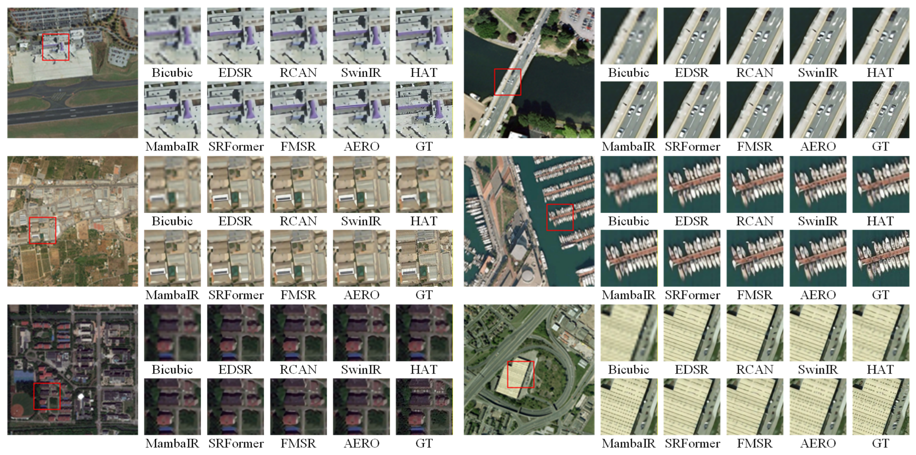
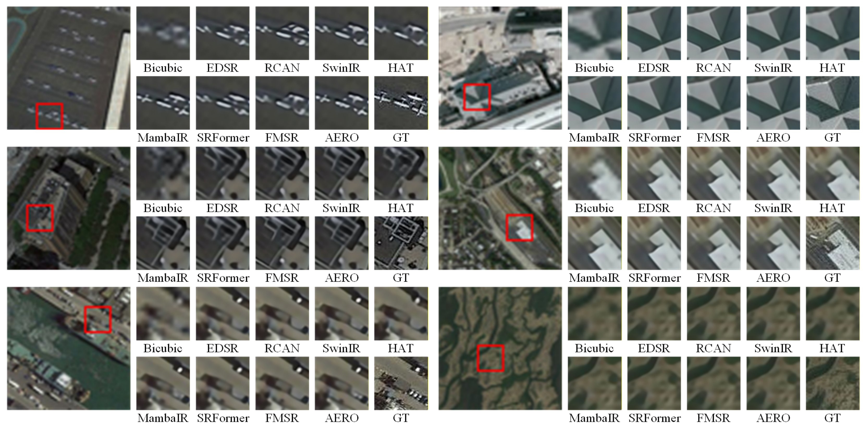
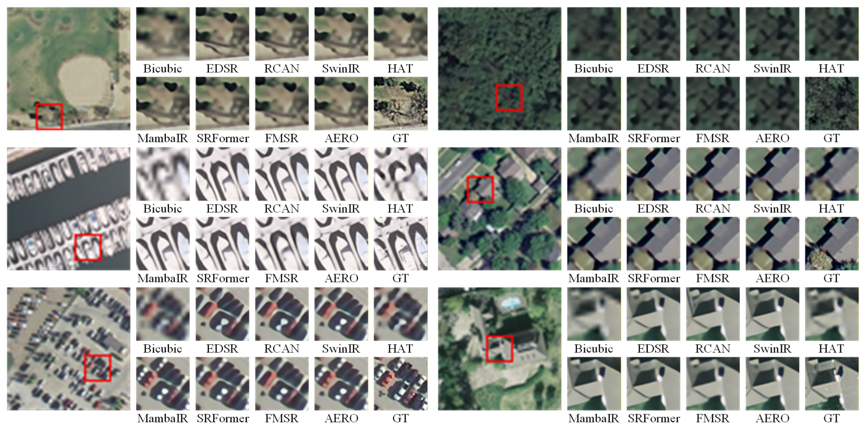
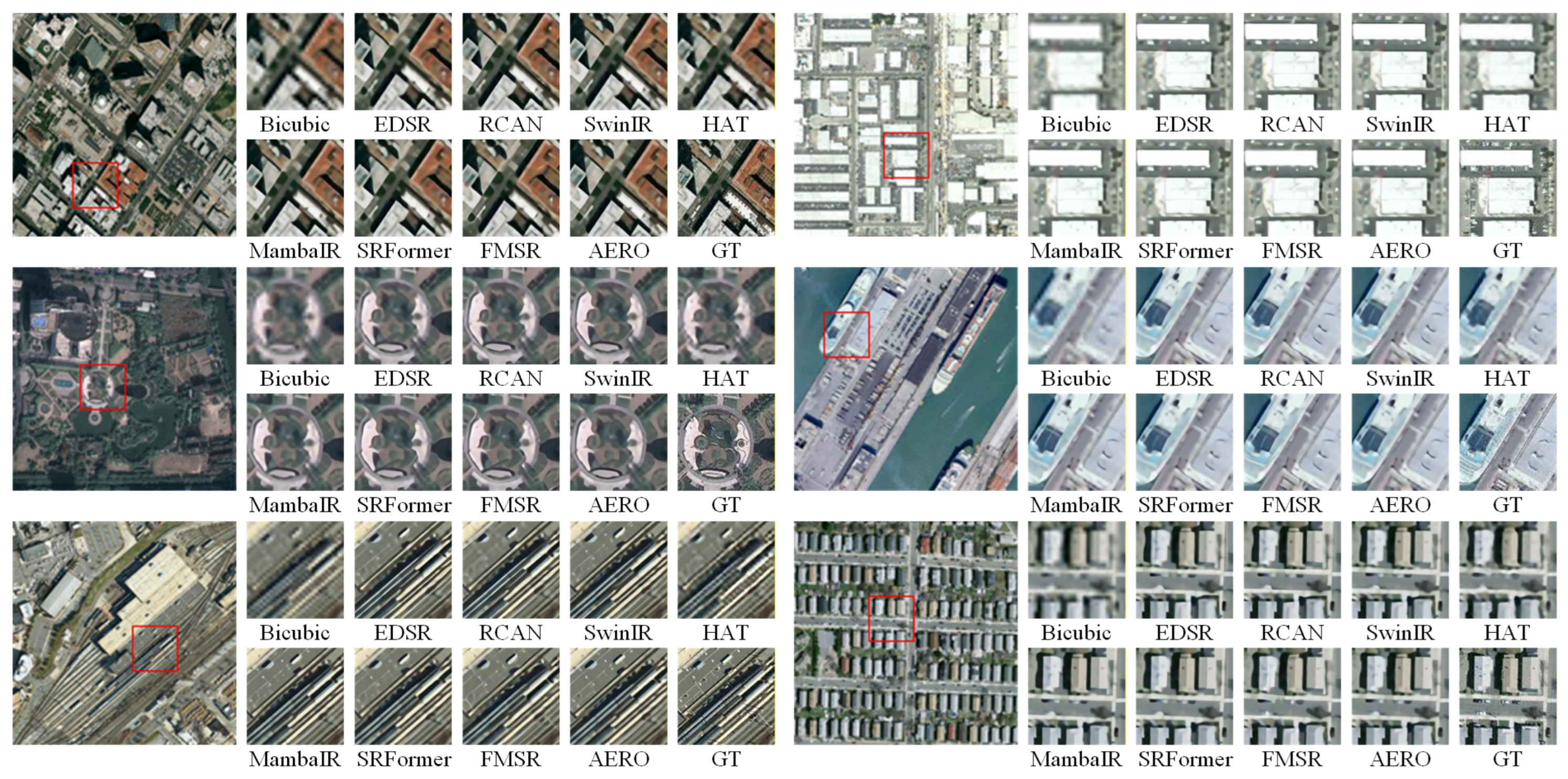
The qualitative visual comparisons (Figure 4, Figure 5, Figure 6 and Figure 7) corroborate these quantitative findings. Baseline CNNs (e.g., EDSR, RCAN) suffer from severe over-smoothing, routinely failing to recover critical high-frequency details. Advanced Transformers and State-Space Models (e.g., HAT, FMSR) improve textural recovery but frequently introduce spurious aliasing or structural distortions on arbitrarily oriented objects, such as angled rooftops or curved viaducts.

Conversely, AERO consistently restores well-defined boundaries and preserves the geometric integrity of both linear topologies and repetitive textures. By effectively isolating critical high-frequency details via the WARG block and explicitly enforcing rotational equivariance through the OFE, AERO mitigates ringing artifacts and maintains crisp separations between dense adjacent structures (e.g., clustered shipping infrastructure) that competing models blur together.

4.3.2. Continuous Arbitrary-Scale Super-Resolution

The fundamental advantage of AERO lies in its Local Implicit Terrain Operator (LITO), enabling it to break free from fixed grids and infer non-integer scales seamlessly. To demonstrate this capability, we benchmark AERO against leading continuous Implicit Neural Representations (INRs), including LIIF, OverNet, CiaoSR, SADN, FunSR, and NeurOp-Diff. We evaluate performance across both in-distribution scales (trained directly: $\times 2.0,\times 3.0,\times 4.0$) and out-of-distribution scales (unseen during training: $\times 5.0$ to $\times 10.0$).

As evidenced by

Table 3. Quantitative comparison of continuous arbitrary-scale SR models on the AID dataset. Performance is evaluated across both in-distribution (seen during training) and extreme out-of-distribution (unseen) continuous scales. The best, second-best, and third-best results are highlighted in bold, underline, and double underline, respectively.

Method	In-Distribution														Out-of-Distribution
	2.0			2.5			3.0			3.1			4.0			5.0			6.0			8.0			10.0
	P	S		P	S		P	S		P	S		P	S		P	S		P	S		P	S		P	S
Bicubic	32.91	0.8991		30.86	0.8460		29.42	0.7953		29.16	0.7847		27.56	0.7120		26.41	0.6537		25.60	0.6132		24.53	0.5624		23.82	0.5373
MetaSR	34.33	0.9150		32.11	0.8711		30.22	0.8256		30.01	0.8198		28.16	0.7512		26.85	0.7022		25.92	0.6612		24.68	0.6012		23.65	0.5611
LIIF	34.45	0.9175		32.22	0.8745		30.34	0.8301		30.12	0.8245		28.29	0.7584		26.96	0.7088		26.04	0.6681		24.81	0.6120		23.72	0.5695
OverNet	34.52	0.9192		32.28	0.8761		30.39	0.8322		30.18	0.8268		28.31	0.7610		27.01	0.7101		26.07	0.6710		24.84	0.6145		23.76	0.5721
CiaoSR	34.55	0.9210		32.32	0.8785		30.43	0.8345		30.22	0.8291		28.36	0.7635		27.05	0.7125		26.11	0.6742		24.89	0.6171		23.81	0.5755
SADN	34.59	0.9221		32.36	0.8801		30.47	0.8361		30.25	0.8305		28.40	0.7645		27.09	0.7135		26.15	0.6755		24.92	0.6189		23.85	0.5781
FunSR	35.24	0.9326		33.15	0.8841		31.17	0.8391		29.50	0.7790		28.58	0.7185		27.56	0.7022		25.49	0.6475		24.45	0.5824		23.55	0.5730
NeurOp-Diff	34.40	0.9161		32.18	0.8732		30.28	0.8288		30.06	0.8222		28.22	0.7544		26.90	0.7055		25.98	0.6655		24.75	0.6085		23.68	0.5655
AERO-Tiny	35.09	0.9275		32.50	0.8852		30.58	0.8399		30.36	0.8325		28.44	0.7652		26.92	0.7118		26.02	0.6722		24.83	0.6186		23.77	0.5763
AERO-Base	35.34	0.9303		32.74	0.8898		30.84	0.8393		30.61	0.8393		28.70	0.7752		27.18	0.7226		26.27	0.6839		25.04	0.6287		23.95	0.5841
AERO-Large	35.50	0.9320		32.92	0.8929		31.02	0.8504		30.79	0.8438		28.89	0.7821		27.37	0.7309		26.46	0.6929		25.21	0.6374		24.10	0.5912

, existing implicit decoders suffer heavily from spectral bias, resulting in rapid PSNR decay as the scale factor increases. By combining explicit sub-pixel offsets in LITO with the frequency priors extracted by the WARG modules, AERO completely overcomes this limitation. AERO-Large achieves state-of-the-art fidelity across every scale. Crucially, in the extreme out-of-distribution scales (e.g., $\times 8.0,\times 10.0$), AERO-Large’s performance gap over baseline INRs significantly widens, mathematically proving that AERO learns a true, robust continuous topographical mapping rather than simply memorizing discrete interpolation matrices.

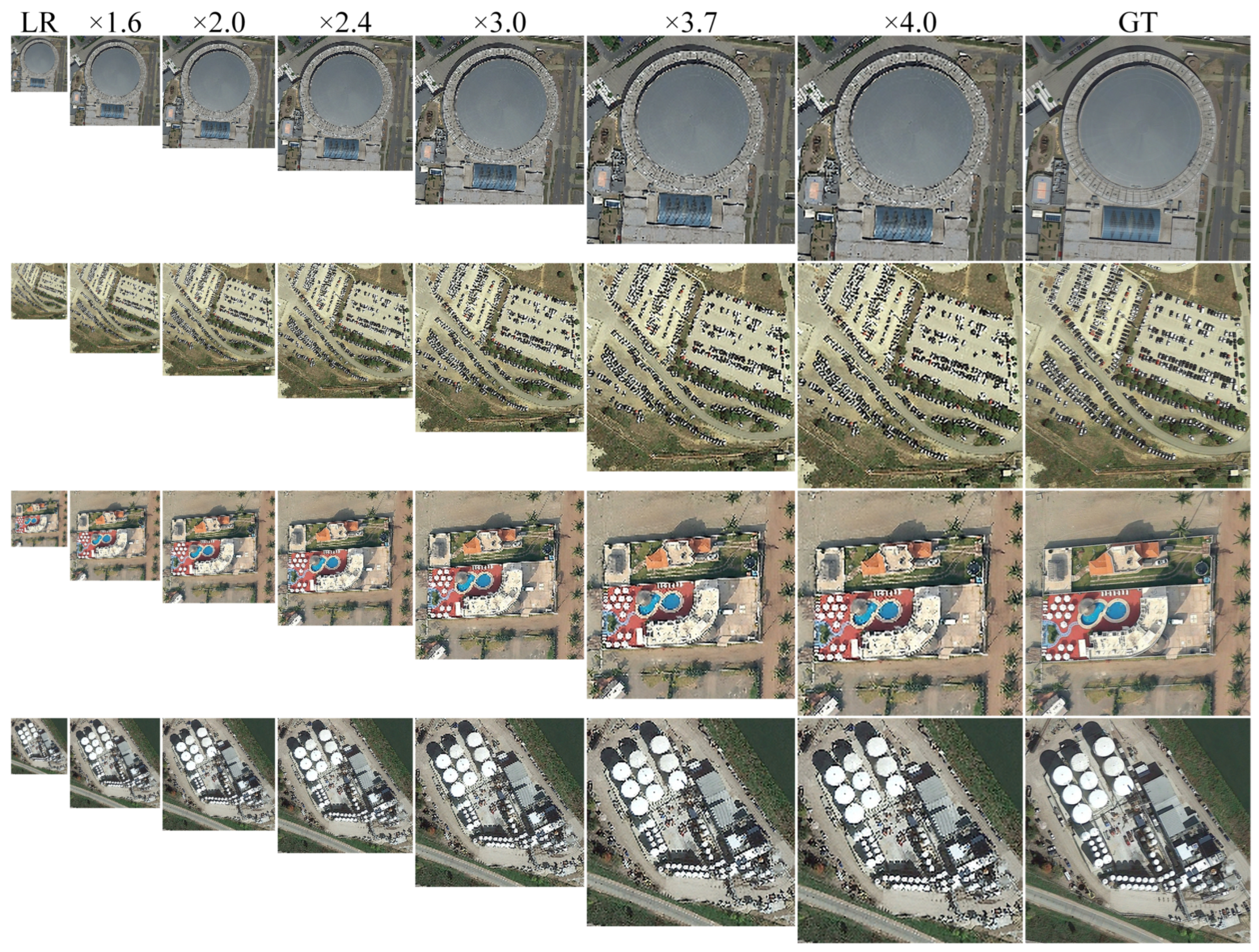
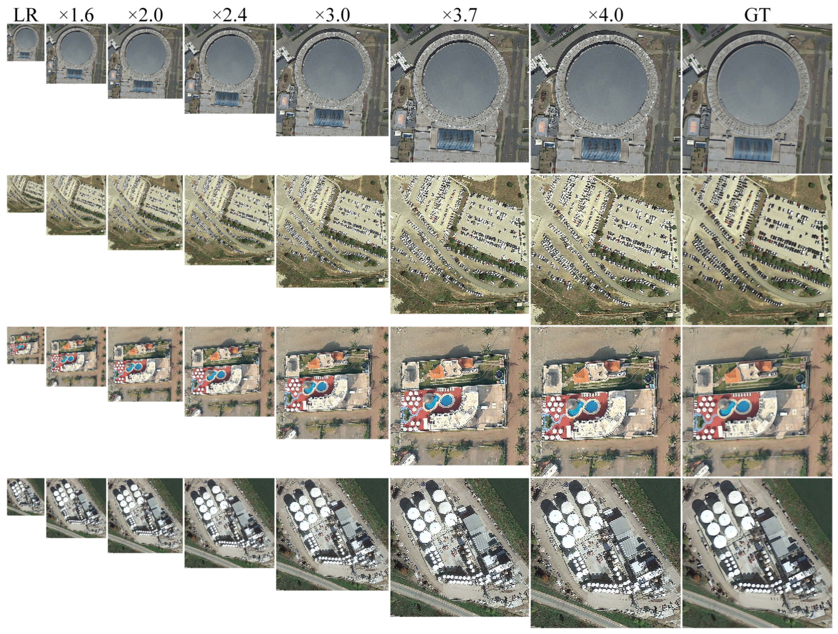
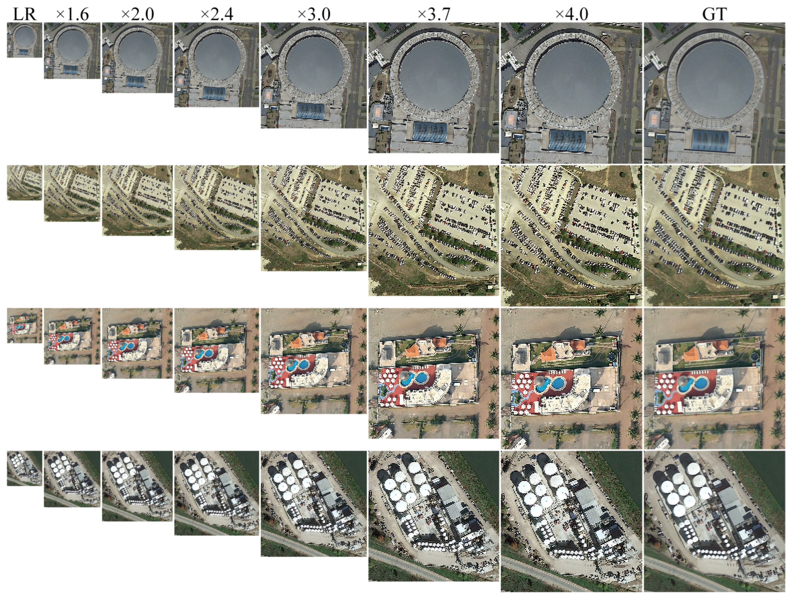
The visual comparisons in Figure 8, Figure 9 and Figure 10 provide a granular validation of these quantitative advantages. We evaluate AERO against recent state-of-the-art continuous frameworks (FunSR and SADN) across a sweeping range of non-integer scales. While the baseline architectures perform adequately at smaller, seen scales, their structural integrity deteriorates rapidly when pushed toward extreme out-of-distribution scale. Specifically, existing implicit decoders struggle to map continuous high-frequency topologies without introducing severe aliasing or spatial blurring. For instance, along the curved boundaries of the circular stadium, FunSR and SADN produce jagged, staircase artifacts that fundamentally distort the intended geometry. Similarly, in densely packed environments such as the parking lot and the industrial storage tanks, the competing methods fail to resolve tight inter-object boundaries. This topological failure causes individual vehicles and distinct cylindrical structures to smear together into unrecognizable, fused masses. Furthermore, in areas with sharp semantic transitions—such as the bright patio umbrellas against the red courtyard—the baselines exhibit noticeable color bleeding and a complete loss of geometric definition.

In stark contrast, AERO effectively circumvents these spectral limitations. By leveraging the sub-pixel spatial awareness embedded within the LITO decoder, our proposed model consistently maintains razor-sharp geometric edges and pristine textural coherence, regardless of the target magnification factor. AERO successfully separates individual parked vehicles, reconstructs smooth concentric curves without aliasing, and prevents color bleeding across sharp boundaries. This exceptional spatial generalization visually proves that AERO learns a robust, continuous topographical mapping, allowing it to render complex aerial features seamlessly at any arbitrary scale.

4.4. Ablation Study

To systematically validate the structural design and mathematical formulations of the proposed architecture, we conduct a comprehensive series of ablation studies. All ablation experiments are evaluated on the AID validation set at a discrete scale factor of $\times 4$. It is critical to note that, while these ablations are quantified on a discrete grid for direct comparison, the structural enhancements inherently apply to the continuous arbitrary-scale domain. Because AERO unifies both paradigms under a single Local Implicit Terrain Operator (LITO), any improvement in deep feature extraction or frequency routing mathematically translates to higher fidelity in the continuous coordinate space.

4.4.1. Effectiveness of Proposed Components

We first perform a macro-architectural component swap to justify the necessity of AERO’s core modules over standard building blocks found in the existing literature. As detailed in

Table 4. Ablation studies isolating the impact of individual architectural components on the proposed AERO framework. Our methods are highlighted in bold.

Components	Model-1 (Base)	Model-2	Model-3	Model-4	Model-5	Model-6	Model-7 (AERO)
Standard $3\times 3$ Conv	✔	×	×	×	×	×	×
Deformable Conv (DCN) [63]	×	✔	×	×	×	×	×
OFE (Ours)	×	×	✔	✔	✔	✔	✔
Standard Strided Pooling	✔	✔	✔	×	×	×	×
Haar DWT/IWT (Ours)	×	×	×	✔	✔	✔	✔
Standard GELU	✔	✔	✔	✔	×	×	×
WKAN (Ours)	×	×	×	×	✔	✔	✔
PixelShuffle (Discrete)	✔	×	×	×	×	×	×
LIIF [45]	×	✔	✔	✔	✔	✔	×
LITO (Ours)	×	×	×	×	×	×	✔
PSNR (dB)	28.51	28.85	29.12	29.28	29.41	29.48	29.55
SSIM	0.7508	0.7672	0.7811	0.7865	0.7904	0.7931	0.7962
Params (M)	0.8624	1.0215	1.1684	1.2412	1.2443	1.2460	1.2465

, we establish a baseline (Model-1) utilizing standard $3\times 3$ convolutions, strided pooling, static GELU activations, and a discrete PixelShuffle upsampler.

Replacing PixelShuffle with LIIF (Model-2) transitions the network to a continuous space. Swapping standard convolutions for Deformable Convolutions (Model-3) improves geometric handling, but explicitly replacing DCN with our Omnidirectional Feature Extractor (Model-4) yields superior PSNR, proving mathematically forced multi-view extraction beats learned offsets for top-down imagery. Sequentially substituting pooling with Wavelets (Model-5) and GELU with WKAN (Model-6) confirms that dynamic frequency routing is strictly required to capture dense geographic textures. Finally, upgrading the generic LIIF decoder to our spatially aware LITO (Model-7) achieves peak performance (29.55 dB), validating the unified AERO pipeline.

4.4.2. Model Capacity and Scaling

To verify that AERO scales predictably and does not rely on massive parameter bloat, we ablate the architectural capacity by modulating the channel dimension (dim) and depth (num_groups, blocks_per_group).

As shown in

Table 5. Model capacity ablation demonstrating the efficiency-to-performance scaling trajectory. The best are highlighted in bold.

Model Variant	Dim	Groups	Blocks	Params (M)	GFLOPs	PSNR (dB)	SSIM	LPIPS
AERO-Tiny	96	4	4	1.246	14.6308	29.552	0.7962	0.3178
AERO-Base	128	6	6	3.7993	21.0869	29.627	0.7989	0.3059
AERO-Large	192	8	8	13.2727	43.0776	29.911	0.8086	0.3039

, AERO-Tiny establishes a highly efficient baseline, achieving competitive fidelity at a fraction of the computational cost (14.6 GFLOPs). Pushing the network capacity to 13.27 M parameters (AERO-Large) systematically enhances the modeling of complex textures, culminating in a peak PSNR of 29.911 dB. By increasing the channel dimension (dim) and the depth of the frequency routing modules (groups and blocks), the network’s representational capacity expands linearly. This structural scaling allows the model to capture increasingly complex, high-frequency geographic textural distributions, directly correlating the increased capacity with improved reconstruction performance. This demonstrates that the WARG modules are robust against gradient saturation and scale efficiently for high-end deployment.

4.4.3. Rotational Equivariance Stress Test

To empirically validate the structural robustness provided by the OFE, we subjected AERO and the Mamba-based state-of-the-art models (FMSR) to a rotational stress test. Input images were mathematically rotated by $0°,90°,180°$, and ${270}^{°}$ prior to inference, with the outputs inversely rotated for alignment evaluation.

Table 6. Rotational robustness ablation. Lower Max Drop (${\Delta }_{Max}$) and Standard Deviation ($\sigma$) indicate superior spatial equivariance. The best results are highlighted in bold.

Model	Metric	$0°$ (Base)	$90°$ Rot.	$180°$ Rot.	$270°$ Rot.	Max Drop (${\Delta }_{\mathit{Max}}$)	Std. Dev. ($\mathit{\sigma }$)
FMSR	PSNR (dB)	29.5990	29.5820	29.5988	29.5809	0.0181	0.0087
	SSIM	0.7942	0.7924	0.7929	0.7923	0.0006	0.0003
AERO w/o OFE	PSNR (dB)	29.8520	29.8450	29.8490	29.8430	0.0090	0.0035
+ Data Aug.	SSIM	0.8050	0.8045	0.8048	0.8043	0.0007	0.0003
AERO (Ours)	PSNR (dB)	29.9170	29.9172	29.9168	29.9162	0.0010	0.0004
	SSIM	0.8086	0.8087	0.8087	0.8087	0.0001	0.0000

proves that the 1D scanning mechanism of State-Space Models (FMSR) suffers from an inherent directional bias, consistently dropping performance at orthogonal angles ($90°$ and $270°$). Furthermore, the newly introduced control group confirms that simply applying identical rotational data augmentation during training to a standard convolutional network (AERO w/o OFE) is insufficient. While data augmentation forces the network to memorize rotational variance—reducing the maximum drop to 0.0090 dB—the rigid spatial grid of standard convolutions still fundamentally lacks symmetric routing, yielding measurable fluctuations. In stark contrast, AERO maintains highly robust discrete rotational invariance. Regardless of input orientation, AERO exhibits a maximum PSNR fluctuation of merely 0.0010 dB ($\sigma =0.0004$), confirming that the explicit multi-view feature fusion of the OFE substantially improves the network against arbitrary satellite orientations beyond what conventional data augmentation can achieve.

4.4.4. Dynamic Frequency Routing via WKAN

We isolate the Kolmogorov–Arnold Network (KAN) inspired activation to prove its efficacy over traditional non-linearities. As detailed in

Table 7. Quantitative ablation of the WKAN activation module, demonstrating the necessity of learnable frequency routing. Our method is highlighted in bold.

Activation Type	Learnable Params	PSNR (dB)	SSIM
Baseline (SiLU)	0	29.35	0.7910
Static Sine	0	29.48	0.7945
WKAN (Ours)	$2\times \dim$	29.55	0.7962

, we compare the fully learnable WKAN against a baseline standard SiLU, and a “Static Sine” variant where the scaling ($\gamma$) and phase ($\beta$) parameters are frozen.

Quantitatively, stripping the high-frequency Sine routing (Baseline SiLU) results in an immediate performance drop, indicating that standard activations over-smooth geographic edges. While forcing a static Sine wave improves metric fidelity, it imposes rigid frequency gating that introduces visible ringing artifacts across homogeneous terrains.

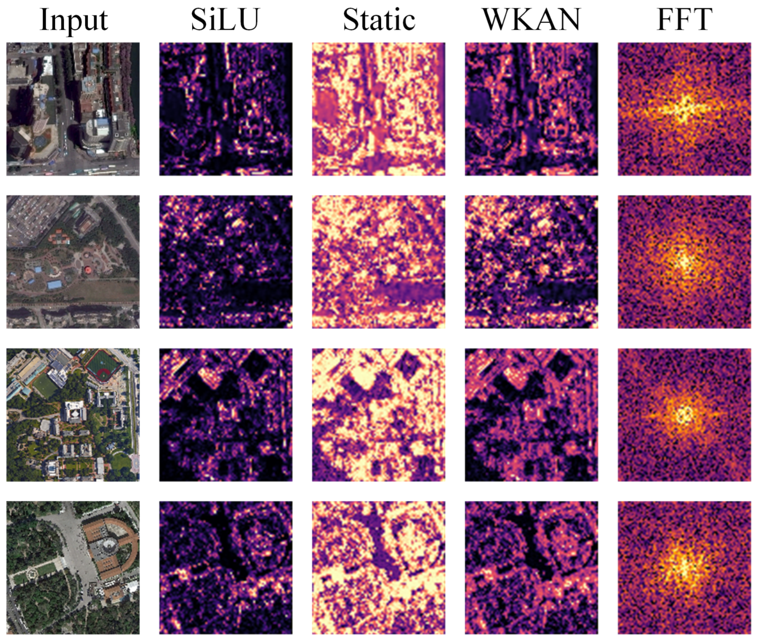
To validate this behavior at the feature level, Figure 11 visualizes the intermediate activation maps across aerial samples from the AID dataset. The visual evidence directly correlates with our quantitative findings by highlighting two distinct failure modes in the baselines. First, the standard SiLU acts as a severe low-pass filter that leads to stark under-activation; the resulting feature maps are predominantly dark, capturing only the most extreme edges while discarding crucial high-frequency textural details. Conversely, the uncalibrated Static Sine variant suffers from over-activation. While it captures structural boundaries, it fails to gate flat regions, erroneously interpreting homogeneous zones (such as grass, water, and pavement) as high-frequency textures. This lack of calibration results in severe noise amplification and spatial ringing.

Our proposed WKAN overcomes both extremes through dynamic gating. By explicitly learning the amplitude and phase shifts, the activation function dynamically adapts to the underlying semantics of the scene. It actively suppresses flat, homogeneous textures—rendering them as dark regions—while preserving sharp, high-intensity activations strictly along critical structural topologies like buildings and roads. Furthermore, the 2D Fast Fourier Transform (FFT) spectrum of the WKAN feature maps exhibits a dense, starburst distribution in the higher frequency bands. This mathematically confirms that WKAN successfully retains the complex, multi-directional high frequencies required for high-fidelity continuous remote sensing.

4.4.5. Spatial Awareness in Implicit Decoding

Finally, we ablate the coordinate framing strategy within the LITO decoder to identify the root cause of topological blurring in continuous networks. As detailed in

Table 8. Quantitative ablation of the spatial coordinate formulation fed to the implicit MLP decoder. Our method is highlighted in bold.

Coordinate Formulation	MLP Inputs	PSNR (dB)	SSIM
Spatially Blind	Feat + 2	28.10	0.7544
Absolute Global	Feat + 4	28.65	0.7620
Relative Sub-Pixel (Ours)	Feat + 4	29.55	0.7962

, we compare our formulation against a spatially blind baseline (relying purely on features and cell scale) and an absolute global coordinate strategy.

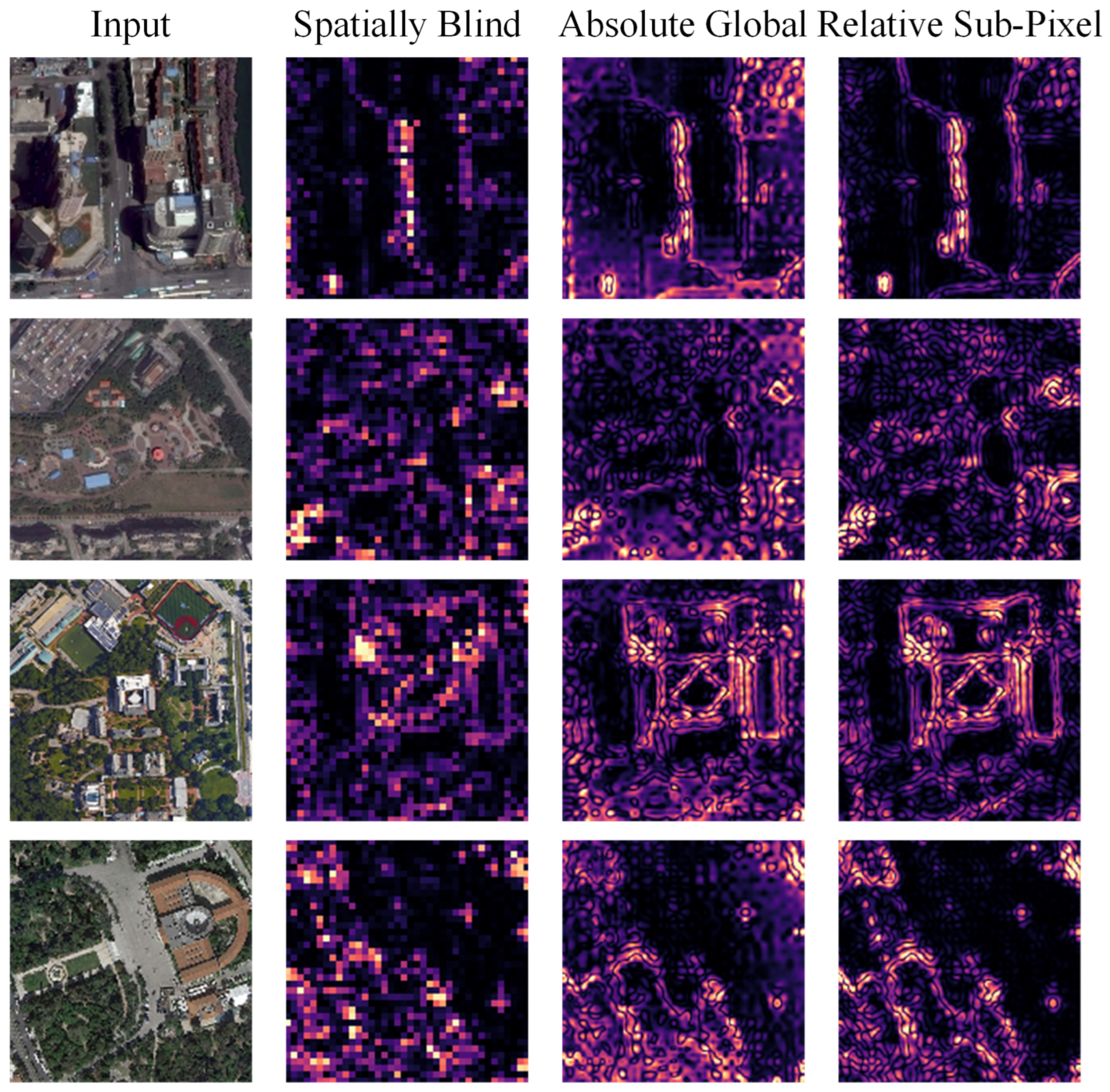
Quantitatively, a spatially blind MLP suffers a severe performance degradation (28.10 dB), entirely failing to resolve boundaries. While feeding absolute global coordinates provides a marginal metric improvement, it still falls significantly short of our proposed method. To diagnose these quantitative gaps, Figure 12 visualizes the isolated high-frequency residual predicted by the MLP under each coordinate strategy, revealing two distinct failure modes in the baselines.

When the network is spatially blind, it is stripped of sub-pixel spatial awareness. The MLP degenerates into a localized color-mapper, producing blocky, pixelated residuals that completely fail to trace fine geometric boundaries. Conversely, while feeding absolute global coordinates provides spatial context, it triggers severe spectral bias. Because the MLP struggles to memorize global absolute locations across the entire macro-image space, it produces out-of-distribution artifacts. This manifests visually as rigid moiré patterns and spurious spatial gradients that disrupt the structural integrity of the scene.

By explicitly projecting the fractional offset within the localized cell, our relative sub-pixel formulation resolves both issues. Rather than attempting global memorization, LITO functions as a dynamic spatial filter. The isolated residual maps demonstrate that this localized approach generates razor-sharp, highly focused topological outlines that perfectly trace complex infrastructure and building edges. This confirms that localized, relative geometry is a mathematical prerequisite for high-fidelity continuous remote sensing.

4.5. Evaluation on Real-World Degraded Imagery

To comprehensively evaluate the generalization capabilities and practical deployment viability of the proposed framework, we further assess the robustness of AERO against real-world, unknown degradations, such as complex sensor noise, atmospheric turbulence, and optical blur. Specifically, we construct a real-world test set by sampling 100 raw, unaligned low-resolution Sentinel-2 satellite patches from the WorldStrat dataset [80]. To strictly evaluate inherent model robustness, the pre-trained networks are directly applied to these degraded inputs without any dataset-specific fine-tuning, domain adaptation, or explicit degradation modeling.

Because real-world satellite acquisitions inherently lack perfectly pixel-aligned high-resolution ground truths, the application of full-reference metrics (e.g., PSNR and SSIM) is mathematically unreliable owing to spatial and temporal misalignments. Consequently, we employ three widely adopted No-Reference Image Quality Assessment (NR-IQA) metrics to objectively quantify reconstruction performance: the Natural Image Quality Evaluator (NIQE), the Blind/Referenceless Image Spatial Quality Evaluator (BRISQUE), and the Average Gradient (AG). For both NIQE and BRISQUE, lower scores correspond to superior perceptual naturalness and reduced artifact generation, whereas a higher AG value signifies sharper textural boundaries and enhanced structural preservation.

As demonstrated in

Table 9. Quantitative evaluation on real-world degraded Sentinel-2 imagery (sampled from WorldStrat) using no-reference metrics. The best results are highlighted in bold. ↓ means smaller is better, ↑ means greater is better.

Method	NIQE ↓	BRISQUE ↓	Average Gradient (AG) ↑
Bicubic	6.245	48.512	3.220
EDSR [16]	5.451	42.120	4.510
SwinIR [28]	4.822	36.884	5.312
FMSR [33]	4.318	32.452	5.840
AERO (Ours)	4.102	31.326	6.125

, conventional discrete networks, including EDSR and SwinIR, exhibit limited robustness against real-world sensor noise. These baseline models frequently amplify underlying degradation artifacts, resulting in deteriorated NIQE and BRISQUE scores. Conversely, AERO achieves the most favorable perceptual scores alongside the highest edge sharpness (AG). This structural robustness is mathematically attributable to the dynamic gating mechanism of the WKAN activation within the WARG blocks. Rather than functioning as a static high-pass filter that indiscriminately amplifies all high-frequency signals—including sensor noise—WKAN operates as an adaptive spatial gate. It effectively suppresses homogeneous background noise, such as atmospheric haze, while selectively preserving and sharpening authentic geographic topologies, thereby demonstrating significant potential for real-world remote sensing applications.

4.6. Deployment Efficiency Analysis

To objectively evaluate the practical engineering deployment value of the proposed framework, we quantitatively assess the inference latency (ms), throughput (FPS), and GPU memory consumption (MB). The evaluation was conducted on an NVIDIA Tesla V100 GPU, processing standard remote sensing input patches. As detailed in

Table 10. Quantitative evaluation of deployment-critical efficiency metrics, including GPU memory, inference time, and throughput (FPS). Our methods are highlighted in bold.

Method	Memory (MB)	Inference Time (ms)	Throughput (FPS)
EDSR	240	76.25	13.11
TransENet	149	87.06	11.49
MambaIR	101	57.24	17.47
FMSR	51	97.32	10.28
MetaSR	167	242.35	4.13
CiaoSR	138	480.68	2.08
AERO-Tiny (Ours)	92	32.64	30.64
AERO-Base (Ours)	153	53.78	18.59
AERO-Large (Ours)	196	81.67	12.24

, we benchmark the three AERO variants against representative discrete (EDSR, TransENet, MambaIR, FMSR) and continuous (MetaSR, CiaoSR) architectures.

The results demonstrate that AERO provides a highly scalable deployment profile. AERO-Tiny achieves real-time throughput at 30.64 FPS with a low memory footprint of 92 MB, making it ideal for resource-constrained edge devices. Meanwhile, the highest-fidelity variant, AERO-Large, operates at 12.24 FPS. Despite its unified discrete-continuous paradigm, it executes faster than the leading Mamba-based baseline, FMSR (10.28 FPS), and significantly outperforms existing continuous implicit networks such as CiaoSR (2.08 FPS), validating its efficiency.

However, it is necessary to explicitly define the operational boundary of continuous decoding. As noted, while LITO executes efficiently at standard integer scales ($\times 2$ to $\times 4$), pushing the arbitrary-scale resolution to extreme magnification factors (e.g., $\times 10$) results in a quadratic increase in continuous coordinate queries. This massive volume of pixel-wise MLP operations induces a localized computational bottleneck, significantly increasing inference latency. Consequently, while AERO supports infinite upscaling, its application at extreme non-integer scales is best suited for interactive Geographic Information Systems (GISs) rendering rather than strict real-time streaming.

5. Discussion

The experimental results indicate that the separation between discrete and continuous super-resolution can be reduced within a unified framework. By considering the geometric and frequency characteristics of remote sensing images, AERO achieves competitive reconstruction performance in both fixed-scale and arbitrary-scale settings while maintaining continuous spatial reconstruction.

From the perspective of discrete feature extraction, the performance of AERO-Large compared with recent Vision Transformers (e.g., HAT, SRFormer) and State-Space Models (e.g., MambaIR, FMSR) suggests that orientation information is important for remote sensing image super-resolution. Previous studies have mainly focused on enlarging the receptive field to capture long-range dependencies. However, the rotational experiments show that large receptive fields or one-dimensional scanning mechanisms may not adequately represent the orientation variations commonly observed in aerial imagery. The Omnidirectional Feature Extractor (OFE) introduces orientation-aware feature extraction at the shallow feature stage. The performance improvements observed in highly structured classes, such as Airport and Viaduct, indicate that explicit modeling of orientation variations can improve reconstruction stability.

The arbitrary-scale experiments also illustrate the influence of spectral bias in Implicit Neural Representations (INRs). Continuous decoders such as LIIF and SADN tend to emphasize low-frequency information, which may result in over-smoothed boundaries and texture degradation at large scaling factors (e.g., $\times 8.0,\times 10.0$). The Wavelet–Arnold Residual Group (WARG) introduces frequency-domain information through wavelet decomposition and dynamic activation functions, while the Local Implicit Terrain Operator (LITO) incorporates relative sub-pixel coordinates during continuous decoding. The ablation results show that these components contribute to preserving high-frequency structures and improving reconstruction quality at non-integer scales.

From the perspective of practical applications, AERO can be applied to both fixed-scale and arbitrary-scale reconstruction tasks. AERO-Tiny provides efficient reconstruction for predefined scale factors, whereas AERO-Large supports continuous zooming in interactive Geographic Information Systems (GISs). The ability to reconstruct images at arbitrary scales without introducing artificial textures may also benefit downstream remote sensing applications, including land-cover classification and disaster assessment.

Several limitations remain. First, the current AERO framework is trained and evaluated using standard bicubic downsampling. While this establishes a rigorous baseline for mathematical fidelity and topological preservation, real-world satellite imagery often suffers from complex, unknown degradations including sensor noise and motion blur. Although the dynamic gating of the WKAN activation theoretically provides some inherent noise-suppression capabilities by dampening homogeneous background activations, the lack of explicit blind degradation modeling remains a limitation for immediate real-world deployment. Second, the reconstruction performance is highly sensitive to the structural hyperparameters of the WARG module; arbitrarily expanding the network depth or channel width beyond the Large variant yields diminishing returns and introduces a risk of overfitting to the training distribution. Third, qualitative observations reveal specific visual failure cases: in scenes dominated by severe cloud shadows or extremely dense, irregular foliage, the wavelet priors occasionally fail to extract coherent high-frequency boundaries, leading to localized topological blurring rather than sharp reconstruction. Although the Haar wavelet effectively separates low-frequency and high-frequency components, it mainly represents horizontal, vertical, and diagonal frequency sub-bands. Consequently, highly irregular or curved geographic structures may not be fully represented. Future work may investigate multi-directional or learnable wavelet transforms to improve the representation of complex spatial structures. Finally, while AERO is optimized for 3-channel optical RGB imagery, its direct application to multispectral or Synthetic Aperture Radar (SAR) data remains challenged by the distinct physical properties of these modalities. Adapting the framework will require significant architectural modifications to handle the complex speckle noise inherent to SAR or to integrate the 3D spectral convolutions necessitated by hyperspectral data.

6. Conclusions

In this paper, we proposed the AERO for remote sensing image super-resolution. The proposed framework combines orientation-aware feature extraction, wavelet-domain feature modeling, and continuous implicit decoding to address both fixed-scale and arbitrary-scale reconstruction tasks. The OFE improves feature representation under orientation variations. The WARG introduces wavelet-domain modeling and dynamic activation functions to preserve high-frequency structures. The LITO performs continuous image reconstruction using relative sub-pixel coordinate information.

Experiments conducted on the AID, UCMerced, NWPU-RESISC45, and WHU-RS19 datasets demonstrate that AERO achieves competitive performance in both fixed-scale and arbitrary-scale super-resolution tasks. Compared with recent Vision Transformer and Mamba-based methods, AERO provides improved reconstruction performance and better preservation of structural details at non-integer scales. The proposed framework also offers multiple model configurations, ranging from AERO-Tiny to AERO-Large, to satisfy different computational requirements. Future work will investigate more flexible frequency representations and the extension of AERO to multi-modal remote sensing data and other remote sensing image restoration tasks.

References

1. Zilberstein, I.; Chien, S. Large-Scale Continual Scheduling and Execution for Dynamic Distributed Satellite Constellation Observation Allocation. arXiv 2026, arXiv:2601.06188. [Google Scholar]
2. Vu, A.D.; Nguyen, K.V.; Bui, B.Q.; Kamel, N. A comprehensive survey of super-resolution remote sensing image datasets: Evolution, challenges, and future directions. IEEE Access 2025, 13, 145350–145372. [Google Scholar] [CrossRef] [Scilit]
3. Ma, Y.; Deng, X.; Wei, J. Land use classification of high-resolution multispectral satellite images with fine-grained multiscale networks and superpixel postprocessing. IEEE J. Sel. Top. Appl. Earth Obs. Remote Sens. 2023, 16, 3264–3278. [Google Scholar] [CrossRef] [Scilit]
4. Al Shafian, S.; Hu, D. Integrating machine learning and remote sensing in disaster management: A decadal review of post-disaster building damage assessment. Buildings 2024, 14, 2344. [Google Scholar] [CrossRef] [Scilit]
5. Wang, D.; Hu, M.; Jin, Y.; Miao, Y.; Yang, J.; Xu, Y.; Qin, X.; Ma, J.; Sun, L.; Li, C.; et al. HyperSIGMA: Hyperspectral intelligence comprehension foundation model. IEEE Trans. Pattern Anal. Mach. Intell. 2025, 47, 6427–6444. [Google Scholar] [CrossRef] [Scilit] [PubMed]
6. Singh, R. Next-Gen Satellite Imaging: Optimizing High-Resolution Remote Sensing with Advanced Stabilization and Data Processing. In Proceedings of the 2025 IEEE International Conference on Recent Advances in Computing and Systems (REACS), Gwalior, India, 19–20 December 2025; pp. 1–6. [Google Scholar]
7. Du, K.; Cheng, Y.; Olsen, P.; Noghabi, S.; Jiang, J. Earth+: On-board satellite imagery compression leveraging historical earth observations. In Proceedings of the 30th ACM International Conference on Architectural Support for Programming Languages and Operating Systems, Rotterdam, The Netherlands, 30 March–3 April 2025; Volume 1, pp. 361–376. [Google Scholar]
8. Dong, C.; Loy, C.C.; He, K.; Tang, X. Learning a deep convolutional network for image super-resolution. In Proceedings of the European Conference on Computer Vision; Springer: Berlin/Heidelberg, Germany, 2014; pp. 184–199. [Google Scholar]
9. Lu, R.; Miao, H.; Hai, X. Efficient remote sensing image super-resolution with residual-enhanced wavelet and key-value adaptation. Front. Remote Sens. 2025, 6, 1718058. [Google Scholar] [CrossRef] [Scilit]
10. Wang, P.; Bayram, B.; Sertel, E. A comprehensive review on deep learning based remote sensing image super-resolution methods. Earth-Sci. Rev. 2022, 232, 104110. [Google Scholar] [CrossRef] [Scilit]
11. Wang, X.; Yi, J.; Guo, J.; Song, Y.; Lyu, J.; Xu, J.; Yan, W.; Zhao, J.; Cai, Q.; Min, H. A review of image super-resolution approaches based on deep learning and applications in remote sensing. Remote Sens. 2022, 14, 5423. [Google Scholar] [CrossRef] [Scilit]
12. Ma, J.; Wang, G.; Zhang, L.; Zhang, Q. Restoration and enhancement on low exposure raw images by joint demosaicing and denoising. Neural Netw. 2023, 162, 557–570. [Google Scholar] [CrossRef] [Scilit] [PubMed]
13. O’shea, K.; Nash, R. An introduction to convolutional neural networks. arXiv 2015, arXiv:1511.08458. [Google Scholar]
14. Dong, C.; Loy, C.C.; He, K.; Tang, X. Image super-resolution using deep convolutional networks. IEEE Trans. Pattern Anal. Mach. Intell. 2015, 38, 295–307. [Google Scholar] [CrossRef] [Scilit] [PubMed]
15. Kim, J.; Lee, J.K.; Lee, K.M. Accurate image super-resolution using very deep convolutional networks. In Proceedings of the IEEE Conference on Computer Vision and Pattern Recognition, Las Vegas, NV, USA, 27–30 June 2016; pp. 1646–1654. [Google Scholar]
16. Lim, B.; Son, S.; Kim, H.; Nah, S.; Mu Lee, K. Enhanced deep residual networks for single image super-resolution. In Proceedings of the IEEE Conference on Computer Vision and Pattern Recognition Workshops, Honolulu, HI, USA, 21–26 July 2017; pp. 136–144. [Google Scholar]
17. Zhang, Y.; Li, K.; Li, K.; Wang, L.; Zhong, B.; Fu, Y. Image super-resolution using very deep residual channel attention networks. In Proceedings of the European Conference on Computer Vision (ECCV), Munich, Germany, 8–14 September 2018; pp. 286–301. [Google Scholar]
18. Zhang, Y.; Tian, Y.; Kong, Y.; Zhong, B.; Fu, Y. Residual dense network for image super-resolution. In Proceedings of the IEEE Conference on Computer Vision and Pattern Recognition, Salt Lake City, UT, USA, 18–23 June 2018; pp. 2472–2481. [Google Scholar]
19. Tai, Y.; Yang, J.; Liu, X.; Xu, C. Memnet: A persistent memory network for image restoration. In Proceedings of the IEEE International Conference on Computer Vision, Venice, Italy, 22–29 October 2017; pp. 4539–4547. [Google Scholar]
20. Dai, T.; Cai, J.; Zhang, Y.; Xia, S.T.; Zhang, L. Second-order attention network for single image super-resolution. In Proceedings of the IEEE/CVF Conference on Computer Vision and Pattern Recognition, Long Beach, CA, USA, 15–20 June 2019; pp. 11065–11074. [Google Scholar]
21. Niu, B.; Wen, W.; Ren, W.; Zhang, X.; Yang, L.; Wang, S.; Zhang, K.; Cao, X.; Shen, H. Single image super-resolution via a holistic attention network. In Proceedings of the European Conference on Computer Vision; Springer: Berlin/Heidelberg, Germany, 2020; pp. 191–207. [Google Scholar]
22. Mei, Y.; Fan, Y.; Zhou, Y. Image super-resolution with non-local sparse attention. In Proceedings of the IEEE/CVF Conference on Computer Vision and Pattern Recognition, Nashville, TN, USA, 20–25 June 2021; pp. 3517–3526. [Google Scholar]
23. Behjati, P.; Rodriguez, P.; Mehri, A.; Hupont, I.; Tena, C.F.; Gonzalez, J. Overnet: Lightweight multi-scale super-resolution with overscaling network. In Proceedings of the IEEE/CVF Winter Conference on Applications of Computer Vision, Waikoloa, HI, USA, 3–8 January 2021; pp. 2694–2703. [Google Scholar]
24. Chenna, D. Evolution of convolutional neural network (CNN): Compute vs memory bandwidth for edge AI. arXiv 2023, arXiv:2311.12816. [Google Scholar]
25. Lei, S.; Shi, Z.; Mo, W. Transformer-based multistage enhancement for remote sensing image super-resolution. IEEE Trans. Geosci. Remote Sens. 2021, 60, 5615611. [Google Scholar] [CrossRef] [Scilit]
26. Chen, H.; Wang, Y.; Guo, T.; Xu, C.; Deng, Y.; Liu, Z.; Ma, S.; Xu, C.; Xu, C.; Gao, W. Pre-trained image processing transformer. In Proceedings of the IEEE/CVF Conference on Computer Vision and Pattern Recognition, Nashville, TN, USA, 20–25 June 2021; pp. 12299–12310. [Google Scholar]
27. Chen, X.; Wang, X.; Zhou, J.; Qiao, Y.; Dong, C. Activating more pixels in image super-resolution transformer. In Proceedings of the IEEE/CVF Conference on Computer Vision and Pattern Recognition, Vancouver, BC, Canada, 17–24 June 2023; pp. 22367–22377. [Google Scholar]
28. Liang, J.; Cao, J.; Sun, G.; Zhang, K.; Van Gool, L.; Timofte, R. Swinir: Image restoration using swin transformer. In Proceedings of the IEEE/CVF International Conference on Computer Vision, Montreal, QC, Canada, 10–17 October 2021; pp. 1833–1844. [Google Scholar]
29. Zhou, Y.; Li, Z.; Guo, C.L.; Bai, S.; Cheng, M.M.; Hou, Q. Srformer: Permuted self-attention for single image super-resolution. In Proceedings of the IEEE/CVF International Conference on Computer Vision, Paris, France, 1–6 October 2023; pp. 12780–12791. [Google Scholar]
30. Aleissaee, A.A.; Kumar, A.; Anwer, R.M.; Khan, S.; Cholakkal, H.; Xia, G.S.; Khan, F.S. Transformers in remote sensing: A survey. Remote Sens. 2023, 15, 1860. [Google Scholar] [CrossRef] [Scilit]
31. Gu, A.; Dao, T. Mamba: Linear-time sequence modeling with selective state spaces. arXiv 2023, arXiv:2312.00752. [Google Scholar]
32. Zhang, Z.; Hu, Z.; Cao, B.; Li, P.; Su, Q.; Dong, Z.; Wang, T. Wiener filter-based Mamba for Remote Sensing Image Super-Resolution with Novel Degradation. IEEE J. Sel. Top. Appl. Earth Obs. Remote Sens. 2025, 18, 26295–26308. [Google Scholar] [CrossRef] [Scilit]
33. Xiao, Y.; Yuan, Q.; Jiang, K.; Chen, Y.; Zhang, Q.; Lin, C.W. Frequency-assisted mamba for remote sensing image super-resolution. IEEE Trans. Multimed. 2024, 27, 1783–1796. [Google Scholar] [CrossRef] [Scilit]
34. Guo, H.; Li, J.; Dai, T.; Ouyang, Z.; Ren, X.; Xia, S.T. Mambair: A simple baseline for image restoration with state-space model. In Proceedings of the European Conference on Computer Vision; Springer: Berlin/Heidelberg, Germany, 2024; pp. 222–241. [Google Scholar]
35. Liu, Y.; Tian, Y.; Zhao, Y.; Yu, H.; Xie, L.; Wang, Y.; Ye, Q.; Jiao, J.; Liu, Y. Vmamba: Visual state space model. Adv. Neural Inf. Process. Syst. 2024, 37, 103031–103063. [Google Scholar] [CrossRef] [Scilit]
36. Yu, W.; Wang, X. Mambaout: Do we really need mamba for vision? In Proceedings of the IEEE/CVF Conference on Computer Vision and Pattern Recognition, Nashville, TN, USA, 11–15 June 2025; pp. 4484–4496. [Google Scholar]
37. Liu, J.; Zhang, L.; Wang, X. Remote Sensing Image Compression via Wavelet-Guided Local Structure Decoupling and Channel–Spatial State Modeling. Remote Sens. 2025, 17, 2419. [Google Scholar] [CrossRef] [Scilit]
38. Zhang, Q.; Ma, S.; Tang, Y.; Zheng, L. Cross-domain continuous-scale remote sensing image super-resolution via meta-weight learning. Sci. Rep. 2026, 16, 6073. [Google Scholar] [CrossRef] [Scilit] [PubMed]
39. Panagiotopoulou, A.; Grammatikopoulos, L.; Kalousi, G.; Charou, E. Sentinel-2 and SPOT-7 images in machine learning frameworks for super-resolution. In Proceedings of the International Conference on Pattern Recognition; Springer: Berlin/Heidelberg, Germany, 2021; pp. 462–476. [Google Scholar]
40. Samadzadegan, F.; Toosi, A.; Dadrass Javan, F. A critical review on multi-sensor and multi-platform remote sensing data fusion approaches: Current status and prospects. Int. J. Remote Sens. 2025, 46, 1327–1402. [Google Scholar] [CrossRef] [Scilit]
41. Chauhan, K.; Patel, S.N.; Kumhar, M.; Bhatia, J.; Tanwar, S.; Davidson, I.E.; Mazibuko, T.F.; Sharma, R. Deep learning-based single-image super-resolution: A comprehensive review. IEEE Access 2023, 11, 21811–21830. [Google Scholar] [CrossRef] [Scilit]
42. An, T.; Huo, C.; Xiang, S.; Pan, C. Combining discrete and continuous representation: Scale-arbitrary super-resolution for satellite images. Remote Sens. 2023, 15, 1827. [Google Scholar] [CrossRef] [Scilit]
43. Sitzmann, V.; Martel, J.; Bergman, A.; Lindell, D.; Wetzstein, G. Implicit neural representations with periodic activation functions. Adv. Neural Inf. Process. Syst. 2020, 33, 7462–7473. [Google Scholar]
44. Hu, X.; Mu, H.; Zhang, X.; Wang, Z.; Tan, T.; Sun, J. Meta-SR: A magnification-arbitrary network for super-resolution. In Proceedings of the IEEE/CVF Conference on Computer Vision and Pattern Recognition, Long Beach, CA, USA, 15–20 June 2019; pp. 1575–1584. [Google Scholar]
45. Chen, Y.; Liu, S.; Wang, X. Learning continuous image representation with local implicit image function. In Proceedings of the IEEE/CVF Conference on Computer Vision and Pattern Recognition, Nashville, TN, USA, 20–25 June 2021; pp. 8628–8638. [Google Scholar]
46. Wu, H.; Ni, N.; Zhang, L. Scale-aware dynamic network for continuous-scale super-resolution. arXiv 2021, arXiv:2110.15655. [Google Scholar]
47. Chen, K.; Li, W.; Lei, S.; Chen, J.; Jiang, X.; Zou, Z.; Shi, Z. Continuous remote sensing image super-resolution based on context interaction in implicit function space. IEEE Trans. Geosci. Remote Sens. 2023, 61, 4702216. [Google Scholar] [CrossRef] [Scilit]
48. Cao, J.; Wang, Q.; Xian, Y.; Li, Y.; Ni, B.; Pi, Z.; Zhang, K.; Zhang, Y.; Timofte, R.; Van Gool, L. Ciaosr: Continuous implicit attention-in-attention network for arbitrary-scale image super-resolution. In Proceedings of the IEEE/CVF Conference on Computer Vision and Pattern Recognition, Vancouver, BC, Canada, 17–24 June 2023; pp. 1796–1807. [Google Scholar]
49. Chen, H.W.; Xu, Y.S.; Hong, M.F.; Tsai, Y.M.; Kuo, H.K.; Lee, C.Y. Cascaded local implicit transformer for arbitrary-scale super-resolution. In Proceedings of the IEEE/CVF Conference on Computer Vision and Pattern Recognition, Vancouver, BC, Canada, 17–24 June 2023; pp. 18257–18267. [Google Scholar]
50. Lee, J.; Jin, K.H. Local texture estimator for implicit representation function. In Proceedings of the IEEE/CVF Conference on Computer Vision and Pattern Recognition, New Orleans, LA, USA, 18–24 June 2022; pp. 1929–1938. [Google Scholar]
51. Wei, M.; Zhang, X. Super-resolution neural operator. In Proceedings of the IEEE/CVF Conference on Computer Vision and Pattern Recognition, Vancouver, BC, Canada, 17–24 June 2023; pp. 18247–18256. [Google Scholar]
52. Xu, Z.; Tang, Y.; Xu, B.; Li, Q. NeurOp-Diff: Continuous remote sensing image super-resolution via neural operator diffusion. In Proceedings of the IEEE/CVF International Conference on Computer Vision, Honolulu, HI, USA, 19–25 October 2025; pp. 12491–12501. [Google Scholar]
53. Rahaman, N.; Baratin, A.; Arpit, D.; Draxler, F.; Lin, M.; Hamprecht, F.; Bengio, Y.; Courville, A. On the spectral bias of neural networks. In Proceedings of the International Conference on Machine Learning, PMLR, Long Beach, CA, USA, 9–15 June 2019; pp. 5301–5310. [Google Scholar]
54. Tancik, M.; Srinivasan, P.; Mildenhall, B.; Fridovich-Keil, S.; Raghavan, N.; Singhal, U.; Ramamoorthi, R.; Barron, J.; Ng, R. Fourier features let networks learn high frequency functions in low dimensional domains. Adv. Neural Inf. Process. Syst. 2020, 33, 7537–7547. [Google Scholar]
55. Wang, X.; Yu, K.; Wu, S.; Gu, J.; Liu, Y.; Dong, C.; Qiao, Y.; Change Loy, C. Esrgan: Enhanced super-resolution generative adversarial networks. In Proceedings of the European Conference on Computer Vision (ECCV) Workshops, Munich, Germany, 8–14 September 2018. [Google Scholar]
56. Wang, X.; Xie, L.; Dong, C.; Shan, Y. Real-esrgan: Training real-world blind super-resolution with pure synthetic data. In Proceedings of the IEEE/CVF International Conference on Computer Vision, Montreal, QC, Canada, 10–17 October 2021; pp. 1905–1914. [Google Scholar]
57. Yue, Z.; Wang, J.; Loy, C.C. Resshift: Efficient diffusion model for image super-resolution by residual shifting. Adv. Neural Inf. Process. Syst. 2023, 36, 13294–13307. [Google Scholar] [CrossRef] [Scilit]
58. Saharia, C.; Ho, J.; Chan, W.; Salimans, T.; Fleet, D.J.; Norouzi, M. Image super-resolution via iterative refinement. IEEE Trans. Pattern Anal. Mach. Intell. 2022, 45, 4713–4726. [Google Scholar] [CrossRef] [Scilit] [PubMed]
59. Mallat, S.G. A theory for multiresolution signal decomposition: The wavelet representation. IEEE Trans. Pattern Anal. Mach. Intell. 2002, 11, 674–693. [Google Scholar]
60. Liu, P.; Zhang, H.; Zhang, K.; Lin, L.; Zuo, W. Multi-level wavelet-CNN for image restoration. In Proceedings of the IEEE Conference on Computer Vision and Pattern Recognition Workshops, Salt Lake City, UT, USA, 18–22 June 2018; pp. 773–782. [Google Scholar]
61. Duan, M.; Qu, L.; Liu, S.; Wang, M. Local implicit wavelet transformer for arbitrary-scale super-resolution. arXiv 2024, arXiv:2411.06442. [Google Scholar]
62. Guo, T.; Seyed Mousavi, H.; Huu Vu, T.; Monga, V. Deep wavelet prediction for image super-resolution. In Proceedings of the IEEE Conference on Computer Vision and Pattern Recognition Workshops, Honolulu, HI, USA, 21–26 July 2017; pp. 104–113. [Google Scholar]
63. Dai, J.; Qi, H.; Xiong, Y.; Li, Y.; Zhang, G.; Hu, H.; Wei, Y. Deformable convolutional networks. In Proceedings of the IEEE International Conference on Computer Vision, Venice, Italy, 22–29 October 2017; pp. 764–773. [Google Scholar]
64. Xia, G.S.; Bai, X.; Ding, J.; Zhu, Z.; Belongie, S.; Luo, J.; Datcu, M.; Pelillo, M.; Zhang, L. DOTA: A large-scale dataset for object detection in aerial images. In Proceedings of the IEEE Conference on Computer Vision and Pattern Recognition, Salt Lake City, UT, USA, 18–23 June 2018; pp. 3974–3983. [Google Scholar]
65. Yang, K.; Pan, A.; Yang, Y.; Zhang, S.; Ong, S.H.; Tang, H. Remote sensing image registration using multiple image features. Remote Sens. 2017, 9, 581. [Google Scholar] [CrossRef] [Scilit]
66. Yang, Y.; Newsam, S. Spatial pyramid co-occurrence for image classification. In Proceedings of the 2011 International Conference on Computer Vision; IEEE: New York City, NY, USA, 2011; pp. 1465–1472. [Google Scholar]
67. Xia, G.S.; Yang, W.; Delon, J.; Gousseau, Y.; Sun, H.; Maître, H. Structural high-resolution satellite image indexing. In Proceedings of the ISPRS TC VII Symposium-100 Years ISPRS, Vienna, Austria, 5–7 July 2010; Volume 38, pp. 298–303. [Google Scholar]
68. Xia, G.S.; Hu, J.; Hu, F.; Shi, B.; Bai, X.; Zhong, Y.; Zhang, L.; Lu, X. AID: A benchmark data set for performance evaluation of aerial scene classification. IEEE Trans. Geosci. Remote Sens. 2017, 55, 3965–3981. [Google Scholar] [CrossRef] [Scilit]
69. Cheng, G.; Han, J.; Lu, X. Remote sensing image scene classification: Benchmark and state of the art. Proc. IEEE 2017, 105, 1865–1883. [Google Scholar] [CrossRef] [Scilit]
70. Wei, Y.; Wang, Z.; Xu, M. Road structure refined CNN for road extraction in aerial image. IEEE Geosci. Remote Sens. Lett. 2017, 14, 709–713. [Google Scholar] [CrossRef] [Scilit]
71. Ma, J.; Yan, S.; Zhang, L.; Wang, G.; Zhang, Q. Elmformer: Efficient raw image restoration with a locally multiplicative transformer. In Proceedings of the 30th ACM International Conference on Multimedia, Lisboa, Portugal, 10–14 October 2022; pp. 5842–5852. [Google Scholar]
72. Ma, J.; Hu, S.; Zhang, X.; Wan, J.; Huang, J.; Zhang, L.; Khan, S. EvoIR: Towards All-in-One Image Restoration via Evolutionary Frequency Modulation. arXiv 2025, arXiv:2512.05104. [Google Scholar]
73. Zhao, H.J.; Lu, X.P.; Di, K.C. Arbitrary-Scale Planetary Remote Sensing Super-Resolution via Adaptive Frequency–Spatial Neural Operator. Remote Sens. 2025, 17, 3718. [Google Scholar] [CrossRef] [Scilit]
74. Ma, J.; Cheng, T.; Wang, G.; Zhang, Q.; Wang, X.; Zhang, L. Prores: Exploring degradation-aware visual prompt for universal image restoration. arXiv 2023, arXiv:2306.13653. [Google Scholar]
75. Feng, X.; Zhang, W.; Su, X.; Xu, Z. Optical remote sensing image denoising and super-resolution reconstructing using optimized generative network in wavelet transform domain. Remote Sens. 2021, 13, 1858. [Google Scholar] [CrossRef] [Scilit]
76. Yang, J.; Zhao, Y.Q.; Chan, J.C.W.; Xiao, L. A multi-scale wavelet 3D-CNN for hyperspectral image super-resolution. Remote Sens. 2019, 11, 1557. [Google Scholar] [CrossRef] [Scilit]
77. Wang, Z.; Bovik, A.C.; Sheikh, H.R.; Simoncelli, E.P. Image quality assessment: From error visibility to structural similarity. IEEE Trans. Image Process. 2004, 13, 600–612. [Google Scholar] [CrossRef] [Scilit] [PubMed]
78. Zhang, R.; Isola, P.; Efros, A.A.; Shechtman, E.; Wang, O. The Unreasonable Effectiveness of Deep Features as a Perceptual Metric. In Proceedings of the 2018 IEEE/CVF Conference on Computer Vision and Pattern Recognition, Salt Lake City, UT, USA, 18–23 June 2018; pp. 586–595. [Google Scholar]
79. Loshchilov, I.; Hutter, F. Decoupled Weight Decay Regularization. In Proceedings of the International Conference on Learning Representations, Toulon, France, 24–26 April 2017. [Google Scholar]
80. Cornebise, J.; Orsolic, I.; Kalaitzis, F. Open High-Resolution Satellite Imagery: The WorldStrat Dataset—With Application to Super-Resolution. In Proceedings of the Thirty-Sixth Conference on Neural Information Processing Systems Datasets and Benchmarks Track, Virtual, 28 November 2022. [Google Scholar]
Figure 1. The overall network architecture of the proposed AERO. The network systematically processes images through an OFE, performs frequency-domain modeling via WARG, and constructs continuous-scale outputs using the LITO.
Remotesensing 18 02823 g001
Figure 2. Detailed architectural diagrams of the extraction and decoding components. (a) OFE processes four simultaneous orthogonal rotations to establish spatial equivariance. (b) LITO decodes arbitrary spatial coordinates using explicit relative sub-pixel offsets to overcome topological spectral bias.
Remotesensing 18 02823 g002
Figure 3. Detailed architectural diagram of the WARG. The block utilizes depthwise modeling and dynamic WKAN activations to process wavelet sub-bands, preserving high-frequency geographic details.
Remotesensing 18 02823 g003
Figure 4. Visual comparisons of various state-of-the-art SR models at a scale factor of × 4 on the AID dataset. AERO consistently reconstructs sharper edges and complex geometric structures without introducing aliasing.
Remotesensing 18 02823 g004
Figure 5. Visual comparisons of various state-of-the-art SR models at a scale factor of × 4 on the NWPU-RESISC45 dataset. AERO accurately preserves linear topologies and fine high-frequency textures.
Remotesensing 18 02823 g005
Figure 6. Visual comparisons of various state-of-the-art SR models at a scale factor of × 4 on the UCMerced dataset. Competing models exhibit structural distortions that AERO successfully mitigates.
Remotesensing 18 02823 g006
Figure 7. Visual comparisons of various state-of-the-art SR models at a scale factor of × 4 on the WHU-RS19 dataset. AERO overcomes orientation biases to deliver superior visual fidelity.
Remotesensing 18 02823 g007
Figure 8. Continuous arbitrary-scale super-resolution results generated by AERO (ours). The proposed model consistently preserves razor-sharp geometric edges and high-frequency textural coherence across both in-distribution ( × 1.6 to × 4.0 ) and extreme out-of-distribution ( × 5.0 to × 10.0 ) magnification factors.
Remotesensing 18 02823 g008
Figure 9. Continuous arbitrary-scale super-resolution results generated by FunSR. While the baseline performs adequately at smaller, seen scales, its structural integrity deteriorates rapidly when pushed out-of-distribution, exhibiting severe topological blurring along complex boundaries.
Remotesensing 18 02823 g009
Figure 10. Continuous arbitrary-scale super-resolution results generated by SADN. Similar to other baseline implicit representations, it struggles to maintain spatial generalization at high magnification factors, introducing visible aliasing and geometric distortions.
Remotesensing 18 02823 g010
Figure 11. Feature map visualizations of the activation ablation on the AID dataset. Baseline SiLU heavily under-activates (over-smoothing), while the Static Sine over-activates (noise amplification in flat regions). Our WKAN acts as a dynamic spatial gate, highlighting boundaries while suppressing homogeneous backgrounds. The FFT spectrum confirms the retention of critical high-frequency components.
Remotesensing 18 02823 g011
Figure 12. Isolated MLP residual maps demonstrating the impact of spatial coordinate formulations. The Spatially Blind decoder produces blocky, localized color-mapping, while Absolute Global coordinates introduce spectral bias and moiré artifacts. Our Relative Sub-Pixel formulation (LITO) successfully acts as a dynamic spatial filter, generating razor-sharp topological outlines.
Remotesensing 18 02823 g012