Author Contributions
Conceptualization, Y.Y. (Yifan Yu), S.D. and F.M.; methodology, Y.Y. (Yifan Yu) and S.D.; software, S.D.; validation, Y.Y. (Yifan Yu) and S.D.; formal analysis, Y.Y. (Yifan Yu) and S.D.; investigation, Y.Y. (Yifan Yu), S.D. and Y.Y. (Yang Yang); resources, Y.Y. (Yifan Yu), Y.Y. (Yang Yang) and F.M.; data curation, S.D.; writing—original draft preparation, Y.Y. (Yifan Yu) and S.D.; writing—review and editing, Y.Y. (Yifan Yu), S.D., Y.Y. (Yang Yang) and F.M.; visualization, S.D.; supervision, Y.Y. (Yifan Yu), Y.Y. (Yang Yang) and F.M.; project administration, Y.Y. (Yifan Yu), Y.Y. (Yang Yang) and F.M. All authors have read and agreed to the published version of the manuscript.
Figure 1.
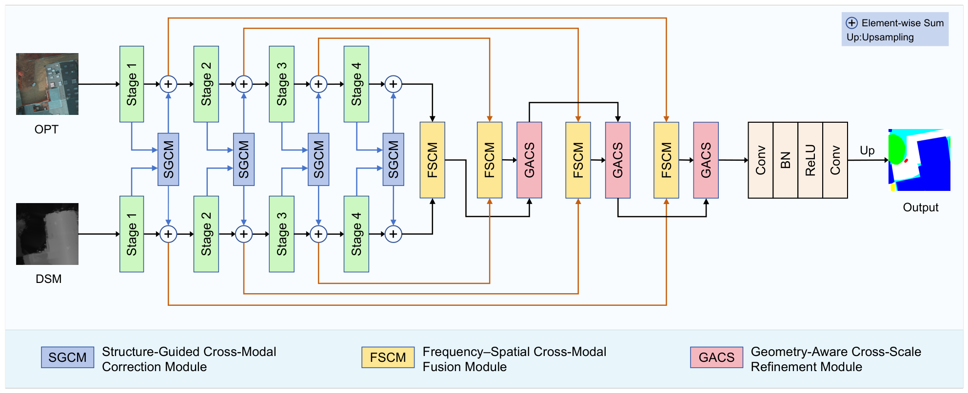
Overall architecture of GCF-Net. SGCM corrects modality-specific features before fusion, FSCM constructs frequency–spatial fused representations, and GACS performs elevation-conditioned refinement during decoding.
Figure 1.
Overall architecture of GCF-Net. SGCM corrects modality-specific features before fusion, FSCM constructs frequency–spatial fused representations, and GACS performs elevation-conditioned refinement during decoding.
Figure 2.
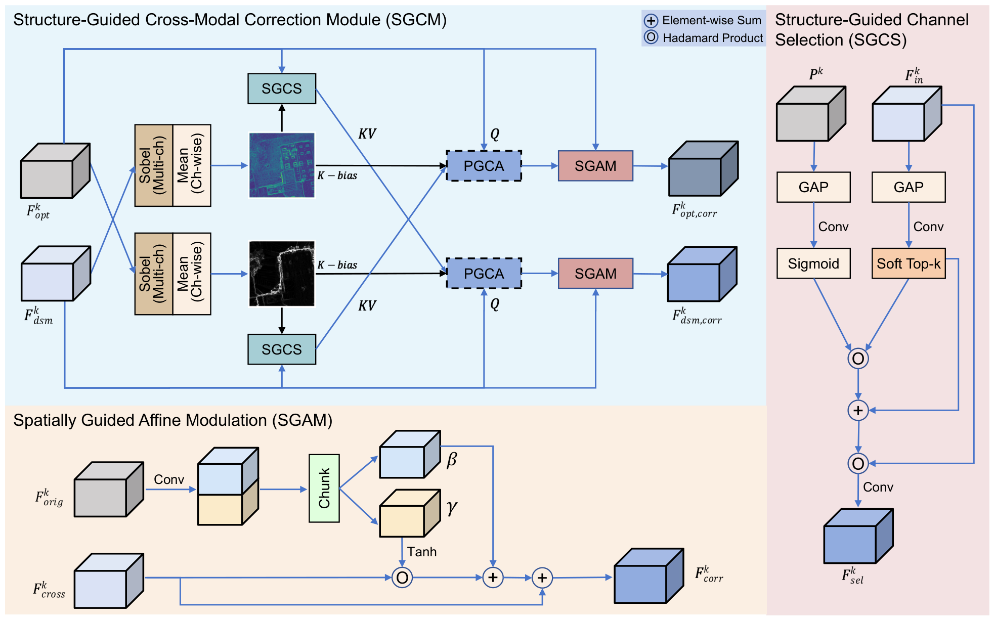
Overview of SGCM. Modality-specific structural priors condition channel selection and cross-attention, while affine modulation regulates the transferred responses.
Figure 2.
Overview of SGCM. Modality-specific structural priors condition channel selection and cross-attention, while affine modulation regulates the transferred responses.
Figure 3.
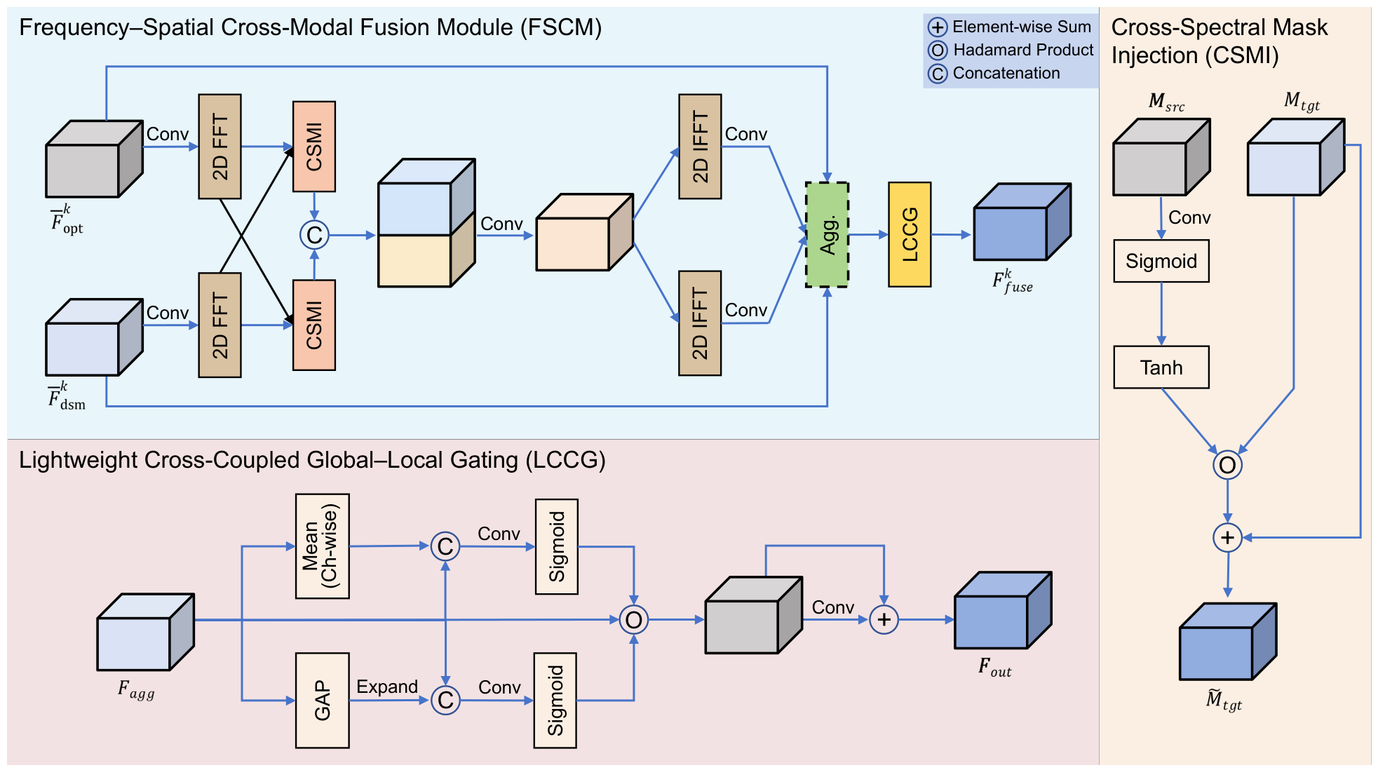
Overview of FSCM. Corrected optical and elevation features undergo bounded cross-modal magnitude modulation, frequency-to-spatial reconstruction, and global–local recalibration to produce the fused representation.
Figure 3.
Overview of FSCM. Corrected optical and elevation features undergo bounded cross-modal magnitude modulation, frequency-to-spatial reconstruction, and global–local recalibration to produce the fused representation.
Figure 4.
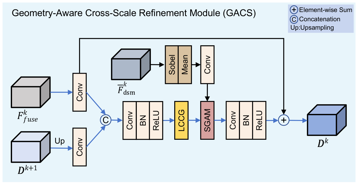
Overview of GACS. Coarse decoded and fused encoder features are integrated, recalibrated by LCCG, and refined using elevation-derived structural guidance.
Figure 4.
Overview of GACS. Coarse decoded and fused encoder features are integrated, recalibrated by LCCG, and refined using elevation-derived structural guidance.
Figure 5.
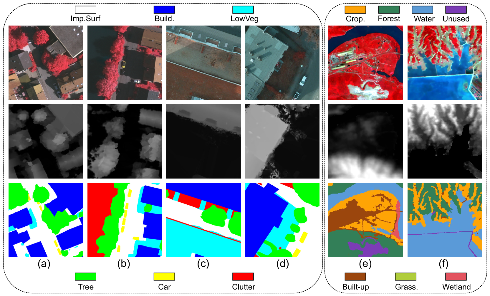
Representative optical images, elevation data, and annotations from the three datasets. Each subfigure shows, from top to bottom, the optical image, elevation data, and corresponding annotation: (a) ISPRS Vaihingen sample 1; (b) ISPRS Vaihingen sample 2; (c) ISPRS Potsdam sample 1; (d) ISPRS Potsdam sample 2; (e) MMHunan sample 1; and (f) MMHunan sample 2.
Figure 5.
Representative optical images, elevation data, and annotations from the three datasets. Each subfigure shows, from top to bottom, the optical image, elevation data, and corresponding annotation: (a) ISPRS Vaihingen sample 1; (b) ISPRS Vaihingen sample 2; (c) ISPRS Potsdam sample 1; (d) ISPRS Potsdam sample 2; (e) MMHunan sample 1; and (f) MMHunan sample 2.
Figure 6.
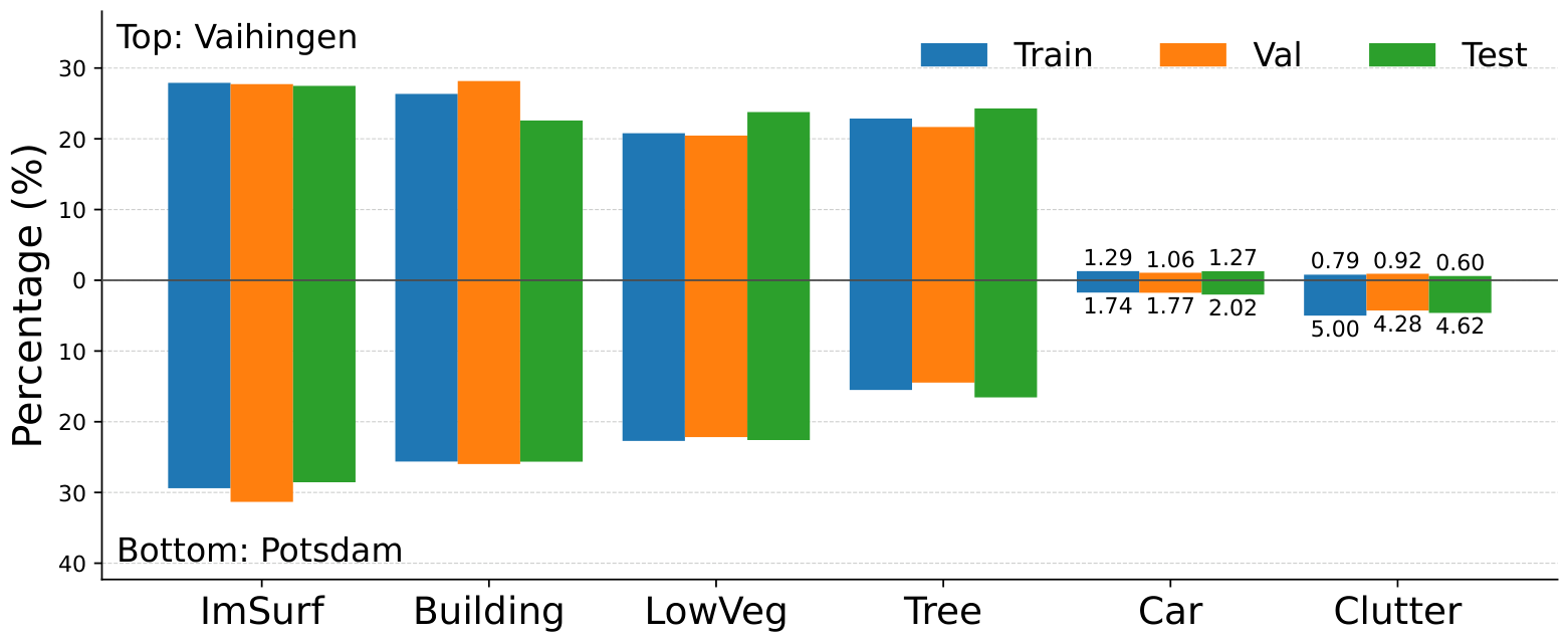
Class distributions across the training, validation, and test splits of ISPRS Vaihingen and Potsdam. The upper and lower panels correspond to Vaihingen and Potsdam, respectively.
Figure 6.
Class distributions across the training, validation, and test splits of ISPRS Vaihingen and Potsdam. The upper and lower panels correspond to Vaihingen and Potsdam, respectively.
Figure 7.
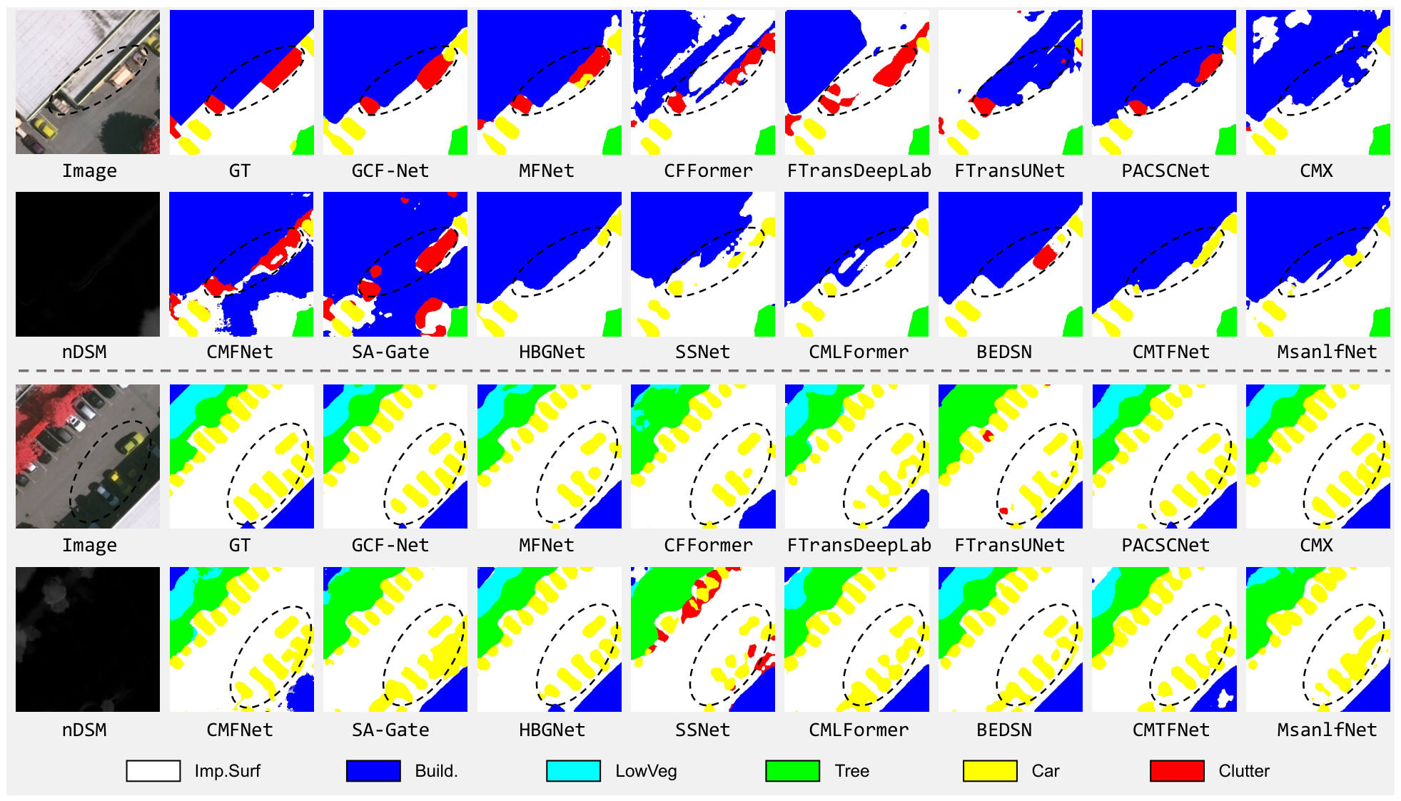
Qualitative comparison on two ISPRS Vaihingen samples. Dashed ellipses highlight representative regions.
Figure 7.
Qualitative comparison on two ISPRS Vaihingen samples. Dashed ellipses highlight representative regions.
Figure 8.
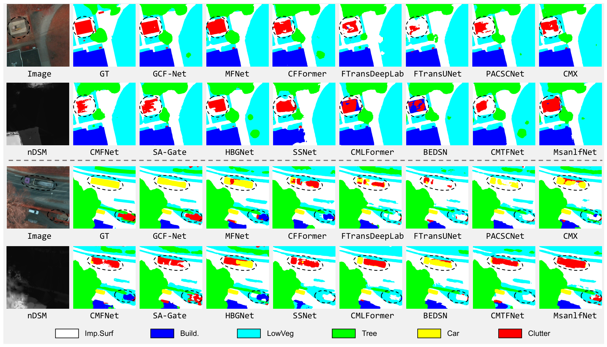
Qualitative comparison on two ISPRS Potsdam samples. Dashed ellipses highlight representative regions.
Figure 8.
Qualitative comparison on two ISPRS Potsdam samples. Dashed ellipses highlight representative regions.
Figure 9.
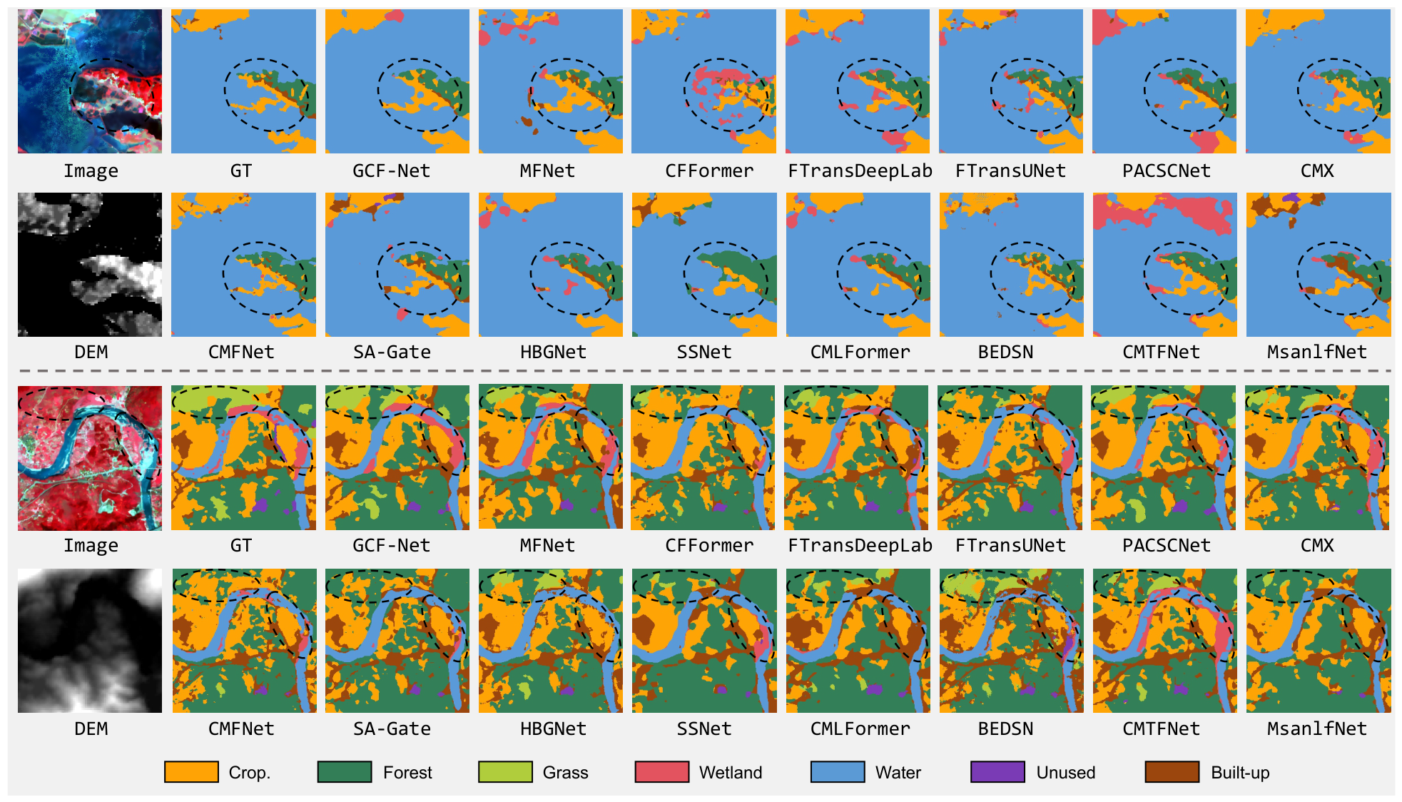
Qualitative comparison on two MMHunan samples. Dashed ellipses highlight representative regions.
Figure 9.
Qualitative comparison on two MMHunan samples. Dashed ellipses highlight representative regions.
Figure 10.
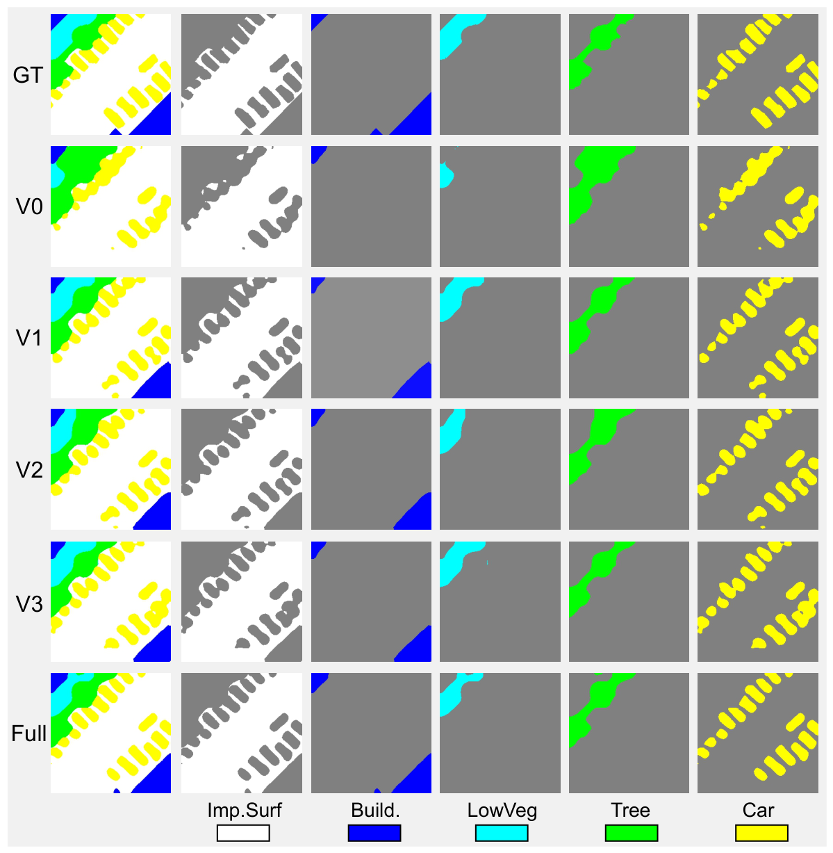
Qualitative comparison of the overall ablation variants on ISPRS Vaihingen. Gray denotes background pixels.
Figure 10.
Qualitative comparison of the overall ablation variants on ISPRS Vaihingen. Gray denotes background pixels.
Figure 11.
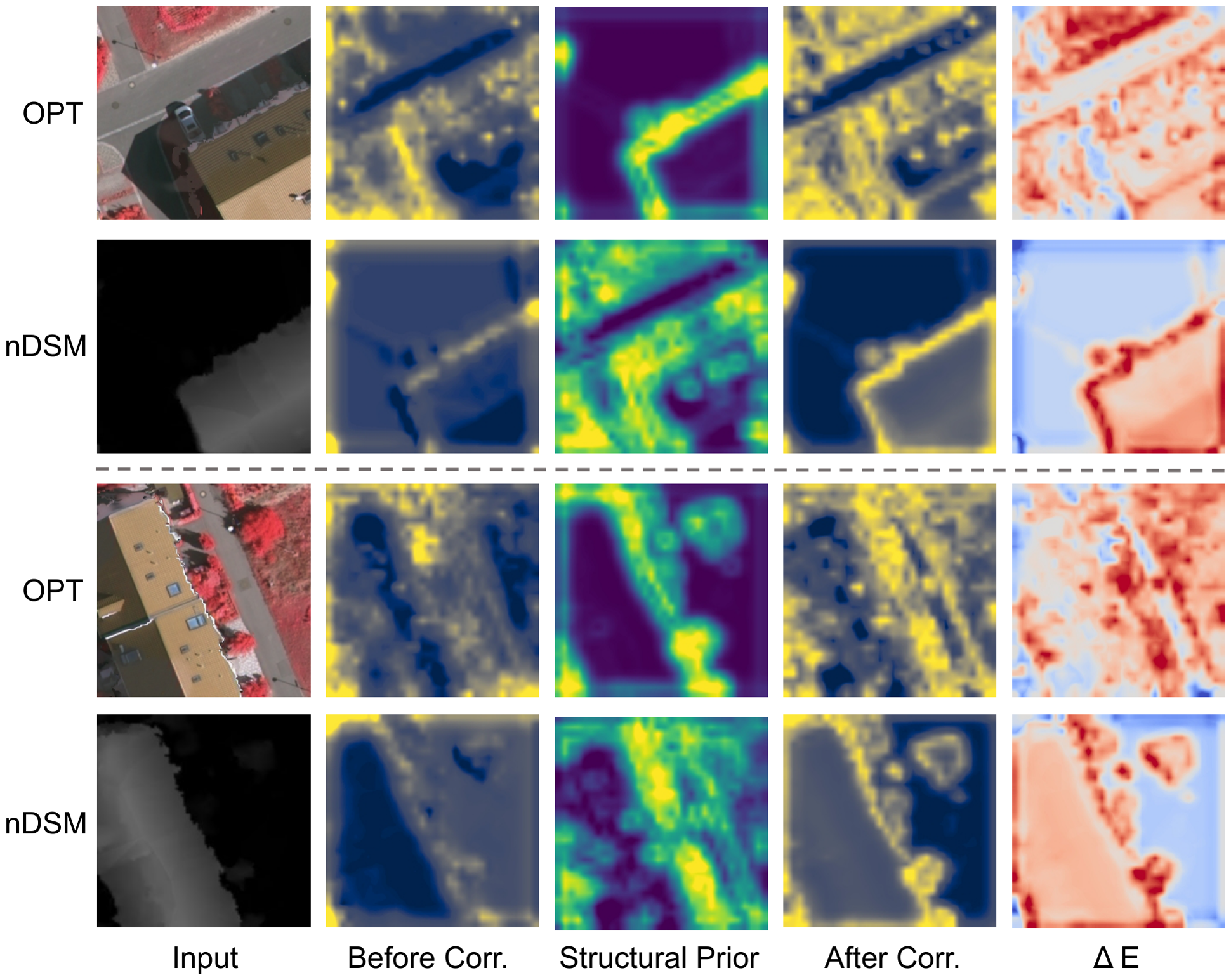
Stage-2 visualization of the SGCM correction process. The before- and after-correction maps show the channel-wise RMS feature energy, while denotes the signed energy change. In the maps, red and blue indicate increased and decreased energy, respectively.
Figure 11.
Stage-2 visualization of the SGCM correction process. The before- and after-correction maps show the channel-wise RMS feature energy, while denotes the signed energy change. In the maps, red and blue indicate increased and decreased energy, respectively.
Figure 12.
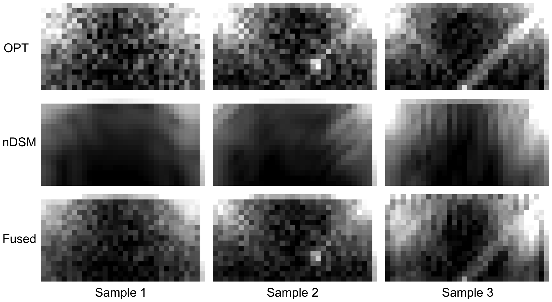
Stage-2 magnitude spectra of the optical, nDSM, and fused FSCM representations for three Vaihingen samples. A shared grayscale normalization is used within each sample.
Figure 12.
Stage-2 magnitude spectra of the optical, nDSM, and fused FSCM representations for three Vaihingen samples. A shared grayscale normalization is used within each sample.
Table 1.
Stage-specific roles of the main components in GCF-Net.
Table 1.
Stage-specific roles of the main components in GCF-Net.
| Module | Stage | Target Issue | Distinct Function |
|---|
| SGCM | Pre-fusion | Cross-modal structural inconsistency | Structure-conditioned correction of modality-specific features. |
| FSCM | Fusion | Frequency–spatial response imbalance | Bounded cross-modal magnitude conditioning and spatial recalibration. |
| GACS | Decoder | Decoder-stage structural attenuation | Elevation-conditioned refinement of fused decoder features. |
Table 2.
Patch extraction settings and final sample counts.
Table 2.
Patch extraction settings and final sample counts.
| Dataset | Patch Size | Overlap | Train | Val | Test |
|---|
| Vaihingen | 256 × 256 | 25% | 5756 | 789 | 780 |
| Potsdam | 512 × 512 | 25% | 11,700 | 1350 | 1350 |
| MMHunan | 256 × 256 | 0% | 400 | 50 | 50 |
Table 3.
Quantitative comparison on ISPRS Vaihingen (%). Best and second-best results are bold and underlined; mIoU5 excludes clutter, whereas mIoU6 includes it.
Table 3.
Quantitative comparison on ISPRS Vaihingen (%). Best and second-best results are bold and underlined; mIoU5 excludes clutter, whereas mIoU6 includes it.
| Method | IoU | mIoU5 | mIoU6 | mF1 | OA | Kappa |
|---|
| Imp. Surf. | Build. | LowVeg | Tree | Car | Clutter |
|---|
| Multimodal methods |
| GCF-Net (ours) | 82.73 | 89.08 | 70.26 | 77.20 | 66.51 | 48.43 | 77.16 | 72.37 | 83.26 | 88.40 | 84.69 |
| MFNet [17] | 82.00 | 88.15 | 69.36 | 76.03 | 61.45 | 42.75 | 75.40 | 69.96 | 81.35 | 88.37 | 84.64 |
| CFFormer [13] | 79.22 | 83.71 | 68.62 | 76.96 | 50.54 | 29.58 | 71.81 | 64.77 | 76.78 | 86.57 | 82.24 |
| FTransDeepLab [21] | 80.02 | 85.64 | 68.15 | 76.36 | 50.11 | 28.12 | 72.06 | 64.73 | 76.58 | 86.78 | 82.53 |
| FTransUNet [7] | 78.98 | 84.01 | 69.28 | 77.22 | 54.50 | 35.17 | 72.80 | 66.53 | 78.53 | 86.79 | 82.53 |
| PACSCNet [11] | 80.51 | 87.17 | 69.81 | 77.01 | 64.02 | 46.58 | 75.70 | 70.85 | 82.20 | 87.67 | 83.72 |
| CMX [28] | 79.84 | 85.14 | 68.92 | 76.58 | 62.15 | 25.32 | 74.53 | 66.32 | 77.69 | 86.93 | 82.73 |
| CMFNet [12] | 80.94 | 87.59 | 68.96 | 76.68 | 60.59 | 29.27 | 74.95 | 67.34 | 78.67 | 87.41 | 83.38 |
| SA-Gate [27] | 79.14 | 85.58 | 67.69 | 76.82 | 52.89 | 30.74 | 72.42 | 65.48 | 77.40 | 86.60 | 82.32 |
| Unimodal methods |
| HBGNet [40] | 81.92 | 87.83 | 69.18 | 77.04 | 59.58 | 37.47 | 75.11 | 68.84 | 80.26 | 87.86 | 83.96 |
| SSNet [35] | 77.21 | 79.15 | 63.10 | 73.45 | 47.23 | 40.06 | 68.03 | 63.37 | 76.49 | 84.12 | 79.01 |
| CMLFormer [36] | 78.91 | 84.08 | 64.88 | 74.40 | 52.15 | 35.87 | 70.88 | 65.05 | 77.49 | 85.61 | 80.97 |
| BEDSN [42] | 80.91 | 86.53 | 67.31 | 75.49 | 58.99 | 30.93 | 73.85 | 66.69 | 78.36 | 86.90 | 82.69 |
| CMTFNet [37] | 80.73 | 86.77 | 68.52 | 75.18 | 58.56 | 40.27 | 73.95 | 68.34 | 80.11 | 86.99 | 82.82 |
| MsanlfNet [23] | 78.30 | 83.12 | 64.47 | 74.60 | 47.50 | 40.55 | 69.60 | 64.75 | 77.43 | 85.30 | 80.56 |
Table 4.
Quantitative comparison on ISPRS Potsdam (%). Best and second-best results are bold and underlined; mIoU5 excludes clutter, whereas mIoU6 includes it.
Table 4.
Quantitative comparison on ISPRS Potsdam (%). Best and second-best results are bold and underlined; mIoU5 excludes clutter, whereas mIoU6 includes it.
| Method | IoU | mIoU5 | mIoU6 | mF1 | OA | Kappa |
|---|
| Imp. Surf. | Build. | LowVeg | Tree | Car | Clutter |
|---|
| Multimodal methods |
| GCF-Net (ours) | 83.09 | 92.01 | 73.41 | 76.15 | 83.39 | 44.22 | 81.61 | 75.38 | 85.00 | 88.58 | 85.21 |
| MFNet [17] | 80.56 | 91.47 | 71.47 | 75.06 | 82.65 | 34.66 | 80.24 | 72.65 | 82.65 | 87.46 | 83.68 |
| CFFormer [13] | 80.45 | 91.38 | 71.64 | 73.96 | 81.72 | 35.44 | 79.83 | 72.43 | 82.57 | 87.37 | 83.56 |
| FTransDeepLab [21] | 79.02 | 90.74 | 68.72 | 70.08 | 75.69 | 31.55 | 76.85 | 69.30 | 80.24 | 85.98 | 81.74 |
| FTransUNet [7] | 79.27 | 92.19 | 71.81 | 73.51 | 78.76 | 31.99 | 79.11 | 71.26 | 81.55 | 84.12 | 83.16 |
| PACSCNet [11] | 81.34 | 91.26 | 72.40 | 75.63 | 81.08 | 35.34 | 80.34 | 72.84 | 82.84 | 87.92 | 84.23 |
| CMX [28] | 80.75 | 91.18 | 71.03 | 73.36 | 82.84 | 34.67 | 79.83 | 72.31 | 82.42 | 87.23 | 83.38 |
| CMFNet [12] | 80.76 | 90.02 | 70.68 | 73.33 | 82.01 | 33.04 | 79.36 | 71.64 | 81.88 | 86.86 | 82.91 |
| SA-Gate [27] | 79.98 | 90.50 | 69.47 | 72.54 | 79.19 | 34.02 | 78.34 | 70.95 | 81.51 | 86.59 | 82.53 |
| Unimodal methods |
| HBGNet [40] | 82.62 | 90.17 | 72.38 | 75.31 | 83.11 | 36.76 | 80.72 | 73.39 | 83.29 | 87.87 | 84.22 |
| SSNet [35] | 75.18 | 83.56 | 66.34 | 65.66 | 75.99 | 35.91 | 73.35 | 67.11 | 79.18 | 83.25 | 78.21 |
| CMLFormer [36] | 79.78 | 88.70 | 69.89 | 71.08 | 79.87 | 36.51 | 77.86 | 70.97 | 81.74 | 86.33 | 82.19 |
| BEDSN [42] | 80.79 | 90.49 | 71.91 | 74.23 | 83.21 | 38.06 | 80.13 | 73.12 | 83.20 | 87.58 | 83.81 |
| CMTFNet [37] | 78.24 | 86.68 | 70.90 | 74.01 | 78.78 | 37.68 | 77.72 | 71.05 | 81.93 | 86.10 | 81.94 |
| MsanlfNet [23] | 80.09 | 89.12 | 69.82 | 70.74 | 80.43 | 35.32 | 78.04 | 70.92 | 81.61 | 86.35 | 82.21 |
Table 5.
Quantitative comparison on MMHunan (%). Best and second-best results are bold and underlined, respectively.
Table 5.
Quantitative comparison on MMHunan (%). Best and second-best results are bold and underlined, respectively.
| Method | IoU | mIoU | mF1 | OA | Kappa |
|---|
| Crop | Forest | Grass | Wet. | Water | Unused | Built. |
|---|
| Multimodal methods |
| GCF-Net (ours) | 68.92 | 80.27 | 21.85 | 23.32 | 77.24 | 29.49 | 64.52 | 52.23 | 65.07 | 82.42 | 76.07 |
| MFNet [17] | 63.21 | 73.13 | 22.96 | 17.68 | 76.93 | 28.25 | 62.81 | 49.28 | 62.50 | 76.89 | 68.96 |
| CFFormer [13] | 60.20 | 76.13 | 19.85 | 12.52 | 74.71 | 25.91 | 58.59 | 46.84 | 59.65 | 77.43 | 69.86 |
| FTransDeepLab [21] | 61.43 | 78.99 | 12.63 | 6.15 | 71.73 | 20.43 | 58.35 | 44.24 | 55.65 | 78.80 | 71.02 |
| FTransUNet [7] | 66.34 | 80.76 | 15.57 | 12.46 | 74.58 | 23.43 | 63.80 | 48.14 | 59.93 | 81.14 | 73.34 |
| PACSCNet [11] | 66.69 | 76.59 | 27.30 | 18.38 | 75.17 | 22.06 | 63.48 | 49.96 | 62.91 | 80.10 | 73.36 |
| CMX [28] | 63.83 | 78.93 | 22.59 | 5.96 | 71.92 | 21.13 | 63.07 | 46.78 | 58.59 | 79.65 | 72.46 |
| CMFNet [12] | 63.62 | 76.63 | 22.44 | 16.23 | 75.89 | 21.41 | 63.47 | 48.53 | 61.12 | 73.40 | 72.38 |
| SA-Gate [27] | 60.97 | 79.49 | 17.10 | 6.24 | 74.47 | 17.98 | 60.99 | 45.32 | 56.70 | 80.03 | 72.82 |
| Unimodal methods |
| HBGNet [40] | 65.45 | 78.06 | 27.03 | 11.70 | 75.63 | 21.72 | 60.93 | 48.65 | 61.12 | 80.62 | 73.77 |
| SSNet [35] | 60.10 | 74.28 | 7.89 | 15.26 | 76.59 | 14.41 | 54.70 | 43.32 | 54.87 | 77.83 | 69.59 |
| CMLFormer [36] | 59.43 | 77.07 | 8.61 | 11.42 | 77.29 | 22.71 | 57.94 | 44.92 | 56.50 | 78.99 | 71.14 |
| BEDSN [42] | 63.37 | 77.29 | 15.02 | 9.03 | 70.48 | 20.32 | 63.16 | 45.52 | 57.33 | 78.39 | 70.88 |
| CMTFNet [37] | 65.16 | 77.51 | 16.11 | 15.51 | 65.54 | 29.59 | 57.94 | 46.77 | 59.87 | 77.91 | 70.14 |
| MsanlfNet [23] | 55.13 | 76.14 | 9.78 | 1.65 | 75.17 | 12.09 | 51.72 | 40.24 | 50.60 | 77.08 | 68.45 |
Table 6.
Overall component ablation on ISPRS Vaihingen. is relative to V0; best and second-best results are bold and underlined, respectively. A check mark indicates that the corresponding module is enabled.
Table 6.
Overall component ablation on ISPRS Vaihingen. is relative to V0; best and second-best results are bold and underlined, respectively. A check mark indicates that the corresponding module is enabled.
| Variant | Modules | Performance (%) |
|---|
| SGCM | FSCM | GACS | mIoU6 | ΔmIoU6 | mF1 | OA | Kappa |
|---|
| V0 | | | | 66.51 | – | 78.65 | 86.51 | 82.18 |
| V1 | ✓ | | | 70.08 | +3.57 | 81.41 | 87.61 | 83.65 |
| V2 | | ✓ | | 68.08 | +1.57 | 79.41 | 87.82 | 83.89 |
| V3 | | | ✓ | 67.18 | +0.67 | 78.70 | 87.07 | 82.92 |
| Full | ✓ | ✓ | ✓ | 72.37 | +5.86 | 83.26 | 88.40 | 84.69 |
Table 7.
Stage-wise structural-prior ablation on ISPRS Vaihingen. Results are mean ± standard deviation over three seeds, and is relative to w/o Priors. Best and second-best results are bold and underlined, respectively. A check mark indicates that the corresponding structural prior is enabled.
Table 7.
Stage-wise structural-prior ablation on ISPRS Vaihingen. Results are mean ± standard deviation over three seeds, and is relative to w/o Priors. Best and second-best results are bold and underlined, respectively. A check mark indicates that the corresponding structural prior is enabled.
| Variant | Priors | Performance (%) |
|---|
| Enc. | Dec. | mIoU6 | ΔmIoU6 | mF1 | OA | Kappa |
|---|
| w/o Priors | | | | – | | | |
| Enc.-only | ✓ | | | +1.71 | | | |
| Dec.-only | | ✓ | | +0.72 | | | |
| Enc.+Dec. | ✓ | ✓ | | +2.31 | | | |
Table 8.
Comparison of fusion operators on ISPRS Vaihingen. is relative to direct concatenation; best and second-best results are bold and underlined, respectively.
Table 8.
Comparison of fusion operators on ISPRS Vaihingen. is relative to direct concatenation; best and second-best results are bold and underlined, respectively.
| Fusion Operator | mIoU6 | ΔmIoU6 | mF1 | OA | Kappa |
|---|
| Direct concatenation | 66.51 | – | 78.65 | 86.51 | 82.18 |
| Cross-attention | 67.82 | +1.31 | 79.40 | 87.61 | 83.63 |
| FSCM | 68.08 | +1.57 | 79.41 | 87.82 | 83.89 |
Table 9.
Backbone sensitivity on ISPRS Vaihingen. mIoU6 is calculated over all six classes. Best and second-best results are bold and underlined, respectively.
Table 9.
Backbone sensitivity on ISPRS Vaihingen. mIoU6 is calculated over all six classes. Best and second-best results are bold and underlined, respectively.
| Backbone | Backbone Params (M) | Performance (%) |
|---|
| mIoU6 | mF1 | OA | Kappa |
|---|
| PVTv2-B2 | 24.85 | 72.37 | 83.26 | 88.40 | 84.69 |
| Swin-Tiny | 28.29 | 72.31 | 83.41 | 87.99 | 84.14 |
| ConvNeXt-Tiny | 27.82 | 70.97 | 82.17 | 88.12 | 84.31 |
| ResNet-50 | 23.51 | 69.90 | 81.15 | 88.24 | 84.46 |
Table 10.
Sensitivity to optical spectral configuration on ISPRS Potsdam. mIoU6 is calculated over all six classes. Best and second-best results are bold and underlined, respectively.
Table 10.
Sensitivity to optical spectral configuration on ISPRS Potsdam. mIoU6 is calculated over all six classes. Best and second-best results are bold and underlined, respectively.
| Optical Input | Performance (%) |
|---|
| mIoU6 | mF1 | OA | Kappa |
|---|
| IRRG | 75.38 | 85.00 | 88.58 | 85.21 |
| RGB | 74.11 | 84.19 | 87.80 | 84.18 |
| RGBIR | 74.35 | 84.22 | 88.28 | 84.76 |
Table 11.
Robustness to elevation perturbations on ISPRS Vaihingen. Parentheses indicate the mIoU6 change from the clean-input result; best and second-best scores are bold and underlined.
Table 11.
Robustness to elevation perturbations on ISPRS Vaihingen. Parentheses indicate the mIoU6 change from the clean-input result; best and second-best scores are bold and underlined.
| Perturbation | Level | mIoU6 (%) |
|---|
| GCF-Net | PACSCNet | MFNet | CMFNet | FTransUNet |
|---|
| Clean | – | 72.37 | 70.85 | 69.96 | 67.34 | 66.53 |
| Gaussian noise | | 72.01 () | 70.37 () | 69.97 () | 67.29 () | 65.43 () |
| 71.55 () | 69.11 () | 70.00 () | 67.03 () | 63.55 () |
| 71.39 () | 65.48 () | 70.06 () | 60.85 () | 60.80 () |
| Misalignment | 1 pixel | 72.38 () | 70.80 () | 69.97 () | 67.29 () | 66.57 () |
| 3 pixels | 72.34 () | 70.79 () | 69.94 () | 67.15 () | 66.65 () |
| 5 pixels | 72.25 () | 70.73 () | 69.94 () | 66.98 () | 66.34 () |
Table 12.
Computational complexity and inference efficiency. Best and second-best values within each method type are bold and underlined, respectively; lower FLOPs and total parameter counts and higher FPS are preferred.
Table 12.
Computational complexity and inference efficiency. Best and second-best values within each method type are bold and underlined, respectively; lower FLOPs and total parameter counts and higher FPS are preferred.
| Type | Method | Input Size | FLOPs (G) | Total Params (M) | FPS |
|---|
| Multimodal | GCF-Net (ours) | | 18.53 | 81.27 | 30.50 |
| MFNet [17] | | 71.81 | 106.03 | 29.00 |
| CFFormer [13] | | 22.42 | 77.24 | 19.91 |
| Multimodal | FTransDeepLab [21] | | 14.98 | 64.56 | 43.52 |
| FTransUNet [7] | | 59.73 | 203.40 | 34.74 |
| PACSCNet [11] | | 37.86 | 94.05 | 48.80 |
| CMX [28] | | 41.48 | 182.63 | 16.43 |
| CMFNet [12] | | 79.76 | 104.07 | 28.90 |
| SA-Gate [27] | | 41.33 | 110.85 | 59.74 |
| Unimodal | HBGNet [40] | | 59.01 | 30.45 | 68.89 |
| SSNet [35] | | 10.35 | 47.23 | 90.91 |
| CMLFormer [36] | | 6.54 | 21.53 | 89.22 |
| BEDSN [42] | | 85.86 | 22.28 | 90.15 |
| CMTFNet [37] | | 8.56 | 30.07 | 116.53 |
| MsanlfNet [23] | | 6.95 | 34.96 | 57.29 |