A New Method for Extracting Short-Term Deformation Signals from InSAR Time Series and Its Application to the Haihe River ‘23·7’ Basin-Wide Extreme Flood Event

Highlights

What are the main findings?

• We developed a novel InSAR signal extraction approach: a three-stage composite fitting model incorporating linear trend, step, and logarithmic decay terms, which successfully separates short-period transient and decaying deformation signals from noise-contaminated InSAR time series.
• The core inundation zones of the “23·7” Haihe River flood exhibited significant surface uplift (up to 30 mm), with spatial patterns highly consistent with the flood inundation extent.
• Multi-physics forward modeling reveals that elastic loading from surface water only induces a minor subsidence of 2 mm. The observed 30 mm uplift is primarily driven by the pore water rebound effect (up to 36 mm) triggered by rapid groundwater recharge, which outweighs the surface loading effect.

What are the implications of the main findings?

• The proposed signal extraction framework overcomes the limitations of traditional spatiotemporal filtering for capturing high-frequency signals, expanding the application potential of InSAR technology for monitoring extreme short-period hydrological events.
• This study challenges the conventional assumption that flood loading only induces surface subsidence, providing a novel coupled hydrological–geomechanical perspective for understanding the secondary geological effects of extreme floods in alluvial plains.
• The multi-month persistence of post-flood deformation and the near-real-time applicability of the method (with a 12-day latency per Sentinel-1 revisit cycle) jointly provide an operational basis for monitoring secondary geohazard risks following extreme flood events.

Abstract

To address the critical challenge of extracting short-period surface deformation signals induced by extreme floods from InSAR time series, this study focuses on the catastrophic flood that struck the Haihe River Basin in July 2023 (hereinafter referred to as the “23·7” flood, with a total duration of approximately 65 days) and proposes a novel method for transient deformation signal extraction. Using Sentinel-1A satellite data and the PS-InSAR technique, we constructed a multivariate composite fitting function comprising a linear trend term, annual and semi-annual seasonal terms, a step term, and a logarithmic decay term. Through nonlinear least-squares fitting, this approach achieves effective separation of long-term tectonic deformation, seasonal fluctuations, high-frequency noise, and transient flood-related signals. The results show that the W-shaped floodplain east of Xiong’an New Area does not exhibit the expected subsidence induced by water loading but instead features pronounced surface uplift of up to 30 mm. Multi-physics forward modeling reveals the underlying mechanism: the elastic subsidence caused by surface water loading, calculated via the LoadDef spherical loading theory, amounts to only ~2 mm. In contrast, forward modeling based on the GMS three-dimensional groundwater seepage model and the principle of effective stress indicates that the pore water rebound effect can produce surface uplift of up to ~36 mm. The superposition of these two effects is highly consistent with InSAR observations in terms of magnitude, direction, and spatial distribution, confirming that the flood-induced surface deformation is dominated by the pore water rebound effect driven by rapid groundwater recharge, rather than subsidence from water loading. The proposed framework extends the application potential of geodetic techniques for monitoring short-period extreme hydrological events.

1. Introduction

The Haihe River Basin comprises five major tributary systems and covers a total area of approximately 320,600 km², spanning 112–120°E and 35–43°N [1]. It is situated in the temperate East Asian monsoon climate zone of northern North China. Under the influence of summer maritime air masses, the region experiences high humidity and temperature, abundant precipitation, and frequent severe rainstorms. The unstable timing, intensity, and spatial extent of the Pacific subtropical high in summer cause pronounced spatiotemporal variability in precipitation, leading to alternating droughts and floods. The narrow mountain–plain transition zone in the basin favors rapid runoff confluence, which readily generates flash floods characterized by rapid stage fluctuations and high destructive potential. 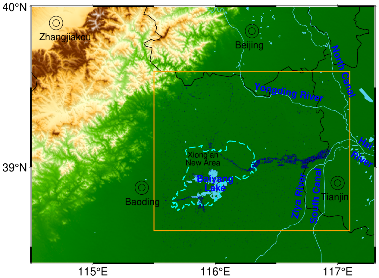As a core political and economic hub in China, the Haihe River Basin is home to the municipalities of Beijing and Tianjin, as well as major cities such as Shijiazhuang, supporting a dense population [2]. Xiong’an New Area was established within the basin on 1 April 2017 (Figure 1). As a key component of China’s national development strategy and a pivotal pilot for modernization transformation, it is designated as a demonstration zone for innovative development embodying the new development philosophy [3]. As a strategic priority for China’s future development, the region has faced recurring flood hazards in recent years. Against this backdrop, conducting refined quantitative research and spatiotemporal analysis of flood-induced surface deformation holds significant scientific and practical value for improving the basin’s capacity to manage flood risks and associated secondary disasters. Specifically, high-precision quantitative observations and physical mechanism analysis of flood-triggered surface deformation can not only capture mechanical processes inaccessible to traditional flood mapping methods but also provide critical data for regional dike safety assessment, secondary geohazard risk evaluation, and post-flood emergency response, making it highly relevant to both scientific research and engineering applications.

Surface deformation induced by the “23·7” flood can be reliably detected using modern geodetic techniques, most notably Interferometric Synthetic Aperture Radar (InSAR). SAR interferometry is recognized as one of the most powerful tools for remote sensing of surface deformation [4]. Unlike optical remote sensing, which depends on sunlight and cloud-free conditions, spaceborne SAR interferometry is widely acknowledged as an active, all-weather observation technique [5]. Time-series InSAR methods derive the spatiotemporal evolution of surface deformation by leveraging information from a stack of SAR interferograms [6]. Initially developed for topographic mapping, InSAR has been widely applied since its emergence [7,8,9,10]. In 1989, Gabriel et al. applied Differential InSAR (D-InSAR) to crustal deformation measurements, demonstrating its sub-centimeter measurement precision [11]. This milestone paved the way for extensive research on D-InSAR-based deformation analysis, establishing InSAR as a mainstream technique for deformation monitoring. However, D-InSAR is highly prone to decorrelation noise and atmospheric delay errors, which substantially compromise measurement accuracy and reliability. To address these limitations, researchers developed multi-temporal SAR time-series approaches grounded in the generation mechanisms and spatiotemporal characteristics of different error sources. The introduction of Permanent Scatterer InSAR (PS-InSAR) in 2000 marked the advent of the Multi-temporal InSAR (MT-InSAR) era [12]. In 2004, Hooper et al. developed a phase-stability-based method for PS point identification, which effectively improved PS density in non-urban natural terrain [13]. Perissin et al. [14] proposed a framework for detecting and characterizing persistent scatterers based on the physical properties of SAR pulse sources. Subsequent studies further expanded MT-InSAR applications. Wang et al. [15] observed and modeled coseismic and postseismic deformation associated with the 2015 Mw 7.8 Nepal earthquake using InSAR and GPS data. Li et al. [16] constructed, analyzed, and validated a high-resolution non-differential atmospheric water vapor model using time-series InSAR observations. Hong et al. [17] investigated postseismic deformation and afterslip evolution of the 2015 Gorkha earthquake by combining InSAR and GPS geodetic observations. Yang et al. [18] monitored land deformation in the Taiyuan region using 36 TerraSAR-X images and the PS-InSAR method. Huang et al. [8] proposed a multi-master pairing strategy analogous to the conventional Small Baseline Subset (SBAS) technique, reducing the standard deviation of time-series results. After decades of development, PS-InSAR has matured into a robust data processing framework, providing a reliable observational basis for investigating surface deformation associated with the “23·7” flood.

In recent years, InSAR has been increasingly applied to flood disaster monitoring [19,20,21,22,23]. One major research direction focuses on flood inundation mapping using SAR intensity data: calm water surfaces cause specular reflection of incident radar beams, appearing as extremely dark regions in SAR imagery [24], which enables the delineation of flood-inundated areas [25,26,27,28,29]. For example, studies have successfully mapped flood inundation extents using Sentinel-1 SAR data for the “23·7” flood in Hebei Province [30], river basin floods in Uttar Pradesh, India [31], and floods triggered by Cyclones Amphan and Yaas [29]. For the catastrophic 2021 “7·20” rainstorm in Henan Province, similar work performed rapid disaster assessments using Sentinel-1 intensity data [27]. However, most of these studies are limited to binary mapping of flood inundation. Few have quantitatively examined the centimeter-scale surface deformation signals induced by floods—a process of greater fundamental and geophysical significance. Our preliminary processing indicates that direct inspection of PS-InSAR deformation time series rarely reveals clear flood-related deformation signals. This is because flood-induced surface deformation is often superimposed on and masked by multiple background signals, including tectonic deformation, groundwater extraction-induced deformation, seasonal periodic deformation, and high-frequency noise. Accurate extraction of flood-associated surface deformation signals carries both geophysical importance and direct relevance to disaster prevention and mitigation practices. The surface deformation field reflects the dynamic response of subsurface aquifers to flood infiltration recharge and can help identify zones prone to foundation instability induced by pore water pressure redistribution. Meanwhile, the spatiotemporal evolution of surface uplift and subsidence in floodplains provides a direct basis for assessing dike and infrastructure safety during and after floods and for developing mitigation strategies for secondary geohazards. This demand is particularly pressing for Xiong’an New Area, a region undergoing large-scale construction and development. Accordingly, the effective separation of short-period transient deformation signals linked to flood processes from complex InSAR time series remains a key unresolved challenge in the field.

Recent advances in time-series InSAR processing have enabled the extraction of increasingly subtle transient deformation signals associated with hydrological processes. Over the past five years, multiple studies have applied advanced signal decomposition methods—including singular spectrum analysis, empirical mode decomposition, and parametric function fitting—to isolate seasonal and short-term hydrological deformation from long-term tectonic and anthropogenic background signals [32,33,34]. For flood events specifically, most recent work has focused on inundation extent mapping using SAR intensity data, with applications across the 2021 Henan rainstorm, cyclone-driven coastal floods, and monsoon-induced basin-wide inundation [27,29,30]. However, quantitative investigations of centimeter-scale flood-induced surface deformation remain limited, particularly for extreme basin-wide events in alluvial plain settings. Furthermore, existing signal extraction methods are generally optimized for seasonal or multi-annual signals, and their ability to reliably recover short-period (1–2 month) flood-related transient deformation remains largely unvalidated.

Flood-associated surface deformation represents a classic loading problem, well suited for analysis using loading theory. Research on loading-induced crustal deformation has a long history. As early as 1911, Love investigated crustal deformation due to surface loads using a self-gravitating Earth model and introduced two dimensionless parameters, h and k, to describe vertical surface displacement and gravitational potential variations [35]. Shida later added a third dimensionless parameter, l, to characterize horizontal displacement [36]. Most subsequent studies have used these three parameters to describe the deformation of a spherically symmetric Earth under surface loading. In 1972, Farrell systematically reviewed the development of loading computation, calculated higher-order Love numbers via numerical integration, and improved the convergence of Green’s functions—particularly in the near field—using multiple approaches including asymptotic solutions, disc factors, and Kummer transformations. For the first time, he derived complete Green’s functions and applied them to compute physical quantities such as displacement, gravity, tilt, and strain [37]. In 2004, Guo et al. derived asymptotic expressions for multiple loading Love numbers by solving the governing ordinary differential equations, achieving one order of magnitude higher accuracy than Farrell’s results [38]. In 2019, Martens et al. summarized conventional surface loading deformation algorithms and released LoadDef (v2019), a comprehensive, well-established open-source software package for computing elastic deformation induced by surface mass loads on a spherically symmetric Earth model [39]. This tool has been widely applied to diverse loading problems, including flood-related surface deformation. In 2021, Fu et al. calculated gravity changes and Coulomb stress changes induced by water impoundment at the Baihetan Reservoir [40]. A 2024 study combining GRACE, GNSS, and glacier elevation data showed that crustal uplift driven by glacier mass loss in the region can reach ~0.5 mm/yr. This signal overlaps with tectonic activity and long-term Glacial Isostatic Adjustment (GIA) signals and must be isolated via refined loading modeling [41].

Quantitative simulation of groundwater level dynamics is critical for understanding the coupling mechanisms between hydrological processes and surface deformation. Early studies relied primarily on analytical methods and physical experiments, which could not fully capture spatiotemporal heterogeneity under complex geological conditions. With advances in numerical simulation, researchers have developed diverse approaches for groundwater system modeling. In 2015, Qiu et al. constructed a numerical model using data from 190 observation wells to characterize the aquifer in the Jilin metropolitan area along the Songhua River, China, and performed transient calibration to validate the results [42]. In 2018, Roozbahani et al. developed a groundwater level prediction model based on Bayesian networks [43] and further ranked water resource management scenarios using multi-criteria decision analysis. In 2019, Shi et al. investigated groundwater dynamics in the Bosten Lake area of the Yanqi Basin, Xinjiang [44]. Among available numerical tools, MODFLOW is widely used for regional groundwater dynamic simulation due to its modular structure and high scalability [45]. Built upon MODFLOW, the Groundwater Modeling System (GMS) is a well-established commercial software package that integrates core modules such as MODFLOW and MT3D, offering a complete workflow from conceptual modeling to 3D visualization. It has been widely applied in studies of groundwater overexploitation and artificial recharge across regions such as the North China Plain and the Yangtze River Delta [46]. In 2019, Aghlmand and Abbasi used GMS MODFLOW to model the aquifer system in the Birjand plain, Iran [47].

Surface deformation induced by groundwater level changes is primarily interpreted via the principle of effective stress, first proposed by Terzaghi in 1923 [48] and widely adopted in research on soil compression and land subsidence. In 1969 and 1975, Riley and Helm, respectively, incorporated aquifer compressibility, storage coefficient, and water level dynamics into numerical models, enabling dynamic simulation of surface deformation driven by groundwater level fluctuations [49,50]. In 1984, Poland [51] systematically established the quantitative relationship between groundwater level changes and the elastic/inelastic deformation of aquifer systems in his review of land subsidence in California’s Central Valley, USA, and proposed an empirical method for estimating surface uplift or subsidence from water level fluctuations. Since the early 2000s, with the maturation of high-precision geodetic techniques such as InSAR and GPS, researchers have started combining observed deformation data with groundwater level models to invert aquifer mechanical parameters and verify the reliability of the pore rebound mechanism [52,53]. In alluvial plains such as the North China Plain, previous studies have confirmed that the pore rebound effect induced by groundwater recharge can significantly offset or mask subsidence signals generated by surface loading [54]. Nevertheless, for extreme floods—high-intensity hydrological events characterized by rapid recharge and recession over a short period—forward modeling of pore rebound based on the effective stress principle has rarely been systematically validated against InSAR observations. Accordingly, there is a pressing need for a spatiotemporally consistent framework for the integrated analysis of groundwater level dynamics and surface deformation.

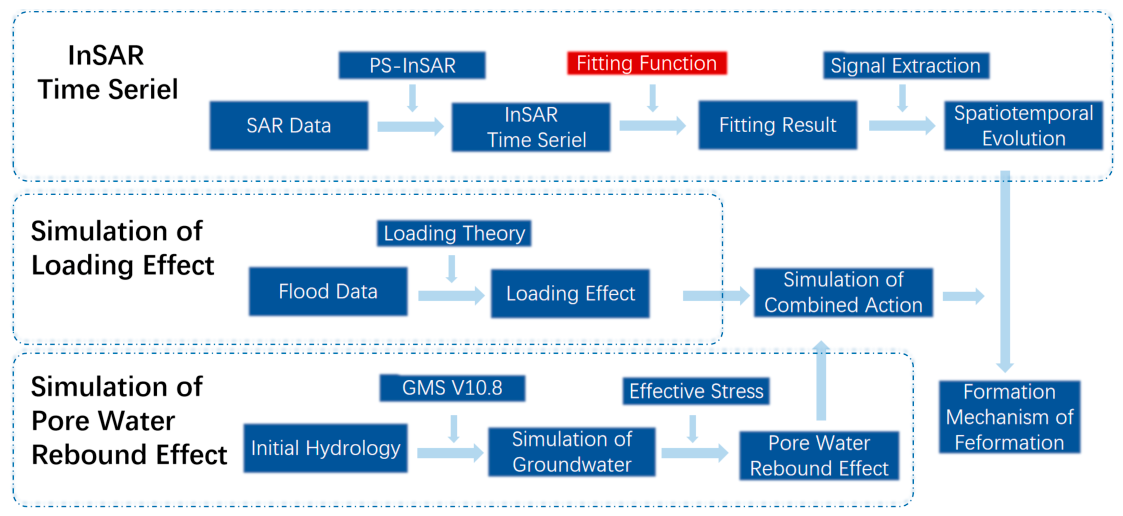
To address these research gaps, this study takes the “23·7” flood as a case study, combining geodetic observations with multi-physics forward modeling to elucidate the complex spatiotemporal evolution of extreme flood-induced surface deformation and its dominant physical mechanism (Figure 2). First, to overcome the challenges posed by the short duration of flood events and the masking of deformation signals by high-frequency noise, we develop a multivariate composite fitting function consisting of a linear trend term, a step term, and a logarithmic decay term, which effectively isolates a high-precision transient deformation field closely linked to flood evolution from PS-InSAR time series. Second, to identify the underlying physical mechanism of the observed deformation, we apply spherical loading theory to compute the elastic deformation field generated by surface water loading. Furthermore, we construct a three-dimensional groundwater seepage model using GMS to quantify dynamic groundwater recharge during the flood period and perform forward modeling of the pore water rebound effect induced by groundwater level rise based on the effective stress principle. Through multi-dimensional cross-validation and comparative analysis between the extracted InSAR observational signals and the results of the two theoretical forward models, this study demonstrates that surface deformation triggered by the “23·7” flood is not simply loading-induced subsidence but a hydro-mechanical coupling response dominated by pore water rebound. This work not only expands the application potential of InSAR for monitoring short-period extreme hydrological events but also provides a novel physical perspective and quantitative assessment framework for understanding the secondary geological effects of flood disasters in alluvial plain regions.

2. Surface Deformation Signals Associated with the “23·7” Flood

2.1. SAR Data and PS-InSAR Processing

The study area is located in the middle and lower reaches of the Haihe River Basin, in the northeastern part of the North China Plain (Figure 1). Bounded by the Taihang Mountains to the west and the Bohai Sea to the east, the basin has a typical temperate monsoon climate with unevenly distributed annual precipitation. Under the influence of the East Asian summer monsoon, rainfall is highly concentrated and severe rainstorms occur frequently, making the region prone to basin-wide flood events. The core impact zone of the “23·7” flood covers the extensive alluvial plain in the lower reaches of the Daqing and Yongding river systems. This plain features gentle topographic relief, with elevations generally below 50 m, a dense river network, and relatively limited drainage capacity. These geomorphic features favor rapid convergence of heavy rainfall over short durations, triggering widespread and long-lasting flood disasters. Xiong’an New Area, established in 2017, lies in the hinterland of the study area (cyan zone in Figure 1). Its planning and development impose stringent requirements on regional flood safety and geohazard risk assessment. This study focuses on the flood-inundated area and its surroundings (orange zone in Figure 1), with the aim of characterizing in detail the spatiotemporal evolution of surface deformation associated with this extreme flood event.

Few continuous Global Navigation Satellite System (GNSS) stations are available within the study area; only Fangshan Station (Fangshan District, Beijing) and Cangxian Station (Cangxian County, Hebei Province) are present, both located relatively far from the actual floodplain. Accordingly, this study uses exclusively C-band Single Look Complex (SLC) data acquired by the Sentinel-1A satellite in Interferometric Wide (IW) swath mode. This dataset provides high spatial resolution and can detect millimeter-scale surface deformation. SLC products are delivered in slant-range geometry, containing focused SAR data along with corresponding satellite orbit and attitude parameters. They feature sufficient signal bandwidth to enable single-look processing in both range and azimuth directions, with phase information stored in complex format. In this work, we apply the PS-InSAR method to process the data and derive the surface deformation time series for the “23·7” floodplain. Sentinel-1A provides enough acquisitions for robust PS-InSAR processing, and data from ascending Track A142 fully cover the entire study area, so no additional Sentinel-1B data are required. The satellite operates at C-band with a radar wavelength of ~5.6 cm. The dataset comprises 90 ascending acquisitions spanning 4 June 2021, to 31 May 2024—approximately two years before the “23·7” flood and one year after, covering a total period of about three years. The orange box in Figure 1 outlines the study area. Due to its geographic extent, two adjacent SAR frames are mosaicked to ensure complete coverage.

The dataset comprises 90 ascending acquisitions spanning 4 June 2021, to 31 May 2024—approximately two years before the “23·7” flood and one year after, covering a total period of about three years. All acquisitions have perpendicular baselines ranging from −121 m to 134 m relative to the common master image. This range is far below the critical baseline for C-band SAR over low-relief alluvial terrain, ensuring robust phase coherence and supporting reliable PS-InSAR processing. The orange box in Figure 1 outlines the study area. Due to its geographic extent, two adjacent SAR frames are mosaicked to ensure complete coverage.

To mitigate decorrelation and retrieve deformation signals from high-coherence point targets, we use Persistent Scatterer InSAR (PS-InSAR) [12,13]. The detailed processing workflow is as follows: (1) Data stacking and co-registration: Using CUDA-enabled stacking scripts from the InSAR Scientific Computing Environment (ISCE) v2.2 [55], we stack and co-register SLC data from the IW1, IW2, and IW3 sub-swaths to a common master image. (2) PS point selection: The co-registered SLC data, baseline information, and geocoded master image are imported into StaMPS v4.1 [56]. Processing follows the single-master PS approach, with the reference SLC image selected by maximizing the sum of coherence coefficients across all interferograms. (3) Phase unwrapping: The Fangshan GNSS station in Beijing is set as the unwrapping reference for ascending Track 142. A 3D unwrapping algorithm is applied to improve unwrapping robustness [57]. (4) Error correction: We estimate and remove spatially uncorrelated errors, including incidence angle error, elevation error, and orbital error. For spatially correlated atmospheric delay noise in slave images (assumed to be temporally uncorrelated), we apply an improved filtering method implemented in StaMPS with a 15-day temporal window. This method dynamically adjusts the temporal window to avoid unintended removal of nonlinear deformation signals, while also supporting detection and correction of phase unwrapping errors. (5) Result output: The displacement time series and mean deformation rates from ascending Track A142 are geocoded and visualized [17]. To balance computational efficiency and cluster memory usage, each image is divided into 60 tiles for parallel processing during PS-InSAR computation, with an output resolution of 50 m.

The StaMPS PS-InSAR algorithm identifies pixels with low phase variance across different land cover types by analyzing the spatial correlation of interferometric phases, without requiring prior assumptions about deformation rates. It can thus capture non-flood deformation signals, including seasonal variations and long-term crustal deformation trends. The temporal filtering window is a critical parameter in StaMPS: it removes high-frequency components from the time series, such as seasonal signals and random noise. In coseismic and postseismic deformation studies, a wider temporal window effectively suppresses noise and seasonal periodic signals, preserving only the coseismic offset and the linear long-term deformation trend. However, flood data from Jiao et al. 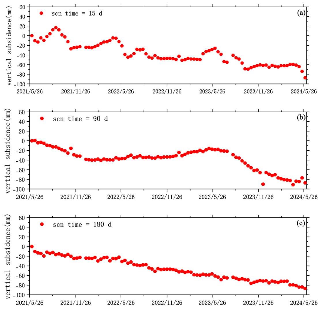[58] indicate that the “23·7” flood lasted only 65 days from onset to substantial recession. This means flood-related deformation signals have similar high-frequency characteristics to seasonal signals and noise, making them difficult to distinguish. Simply widening the temporal filter to suppress high-frequency noise would risk removing the target flood-associated signals. Conversely, the window cannot be too narrow: a filter shorter than the 12-day satellite revisit period would introduce excessive noise, degrade the signal-to-noise ratio (SNR), and undermine subsequent signal extraction. We therefore systematically evaluated signal quality across different temporal window sizes (partial results shown in Figure 3) to preserve flood-related signals while maximizing SNR and ultimately selected a 15-day temporal filtering window.

Precipitation accumulates at the surface to form ponded water, which exerts a vertical load on the land surface. The Sentinel-1A satellite follows a near-polar sun-synchronous orbit and views the surface at a side-looking incidence angle rather than at nadir. For this reason, InSAR measurements are acquired along the line-of-sight (LOS) direction, rather than as the three-component vector data provided by GNSS. This study focuses on vertical surface deformation induced by flooding; since flood loading acts almost entirely in the vertical direction, it is necessary to convert LOS time series into vertical deformation [59].

$$D_k=\psi ·{\displaystyle \frac{-\lambda }{4\pi \cos \theta }}$$

(1)

where $\lambda$ is the radar wavelength of Sentinel-1A (5.6 cm); $\theta$ is local incidence angle of each pixel, defined as the angle between the satellite LOS vector and the local surface normal; $D_k$ is derived vertical surface deformation (mm); and $\psi$ is LOS displacement obtained from StaMPS phase unwrapping (rad).

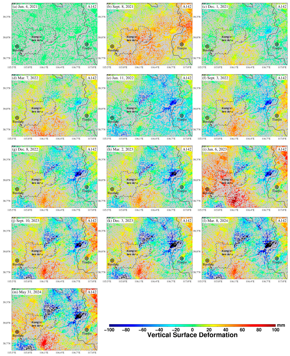
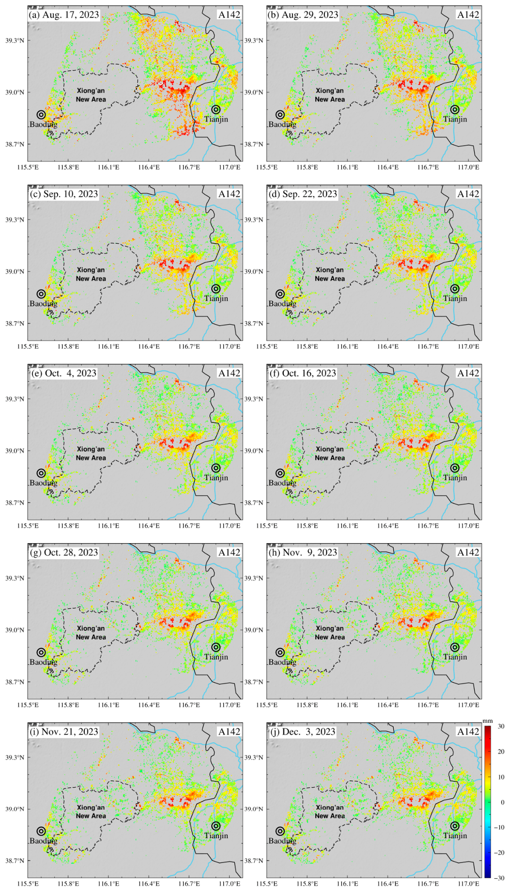
We use the PS-InSAR technique to derive surface deformation time series for the study area. Figure 4 shows cumulative deformation maps for selected representative epochs. Visual inspection reveals two distinct long-term subsidence zones over the observation period: one in Xiong County (northeastern Xiong’an New Area) and another in Bazhou (Langfang, Hebei Province), west of Tianjin. We compared our derived long-term subsidence pattern with results from previous regional InSAR studies [18,54,60] and found high consistency in both the spatial distribution of subsidence zones and the magnitude of subsidence rates, confirming that our PS-InSAR processing is reliable and free of systematic biases introduced during data processing.

As is evident from Figure 4, the raw PS-InSAR deformation field has a highly complex spatial pattern, and flood-related deformation signals cannot be clearly distinguished. This is largely because PS-InSAR observations are superimposed with a mixture of periodic and stochastic deformation components, including tectonic activity, groundwater extraction, anthropogenic activities, and atmospheric delays. Flood-induced deformation signals, by contrast, are relatively weak and can be masked by these background signals. Accordingly, the effective separation and extraction of flood-related surface deformation from complex time series represents a key scientific challenge addressed in this study.

2.2. Fitting Function for Flood-Induced Crustal Deformation

To prevent short-period flood signals from being masked by noise, we set the temporal filtering window to 15 days. However, this narrower window retains more high-frequency interfering signals in the time series, creating challenges for subsequent analysis. The “23·7” flood lasted approximately 65 days from the onset of heavy rainfall to full recession [58]; over such a short duration, random high-frequency noise cannot be sufficiently suppressed simply by widening the temporal filter. We therefore applied a least-squares fitting method to the PS-InSAR time series, followed by detrending and other post-processing steps, to isolate flood-induced surface deformation.

Empirical functions are widely used to fit and model time series when extracting seismic deformation signals from GNSS data. Although both earthquakes and floods induce surface deformation, their underlying mechanisms and spatiotemporal evolution differ substantially. Earthquakes occur when accumulated crustal strain exceeds a threshold, causing crustal failure and instantaneous fault dislocation. After an earthquake, the dislocation is permanent, and the crust continues to deform via postseismic processes such as fault afterslip and mantle viscoelastic relaxation [48].

Floods drive deformation through a fundamentally different mechanism. Intense rainfall produces large volumes of surface water that form floodwater, and the land surface deforms in response to the load imposed by this water body. Over time, ponded floodwater gradually dissipates through infiltration into the subsurface, river runoff, and evaporation. As the water body recedes, its loading effect on the surface progressively weakens. Given these fundamental differences, we developed a three-stage mathematical model to fit surface displacement time series for flood events: Pre-flood stage—Surface deformation is dominated by long-term crustal movement and stratigraphic properties, following a linear trend; Flood onset stage—Water accumulates rapidly at and below the surface, producing a step-like instantaneous deformation response; Post-flood stage—As accumulated water recedes via surface runoff and groundwater flow, deformation gradually recovers and approaches the pre-flood state.

Although simplifying the flood buildup process to a step function is a mathematical idealization, it is physically justified at the temporal resolution of this study. The intense rainfall phase of the “23·7” flood lasted only ~7 days, while the 12-day revisit period of Sentinel-1A ascending Track A142 means the buildup process cannot be captured by multiple time-series samples. Furthermore, the 5 August SLC image, which falls close to the peak flood buildup period, was excluded from the analysis due to severe phase unwrapping errors caused by intense convective weather associated with the remnant vortex of Typhoon Doksuri. As a result, 24 July is the last valid pre-flood observation in the time series; by the next valid acquisition on 17 August, the flood had passed its peak accumulation stage and already begun to recede. InSAR observations therefore cannot resolve the gradual details of flood buildup: the process appears as a discrete jump in the data, from no flooding in one image to fully established inundation in the next. Under these observational constraints, modeling the buildup as a step function is both a practical choice matched to the data’s temporal resolution and a reasonable, necessary approximation of the actual flood process. Artificially imposing a more gradual accumulation function would produce unreliable parameter estimates due to the lack of SAR observations during this period, increasing overfitting risk and reducing the reliability of flood signal extraction.

Flood recession does not follow a simple linear pattern. In the early recession stage, a steep hydraulic gradient drives rapid drainage and high flow velocities, producing a pronounced surface deformation response. As water levels decline, the hydraulic gradient flattens, drainage rates decrease, and the deformation rate gradually stabilizes. From a regional hydrogeological perspective, the lower Haihe River Basin lies within the North China Plain, which is dominated by thick Quaternary sequences of interbedded sand and clay. The aquifer system is characterized by “easy recharge but slow discharge”, expressed as high specific storage, moderate specific yield, and vertical permeability limited by interbedded aquitards [61]. During extreme rainfall recharge events, surface water rapidly infiltrates through the vadose zone to replenish the shallow aquifer. After infiltration, however, the lateral migration and discharge of pore water are strongly constrained by the layered, heterogeneous permeability structure, resulting in typically nonlinear, slow recovery behavior [62].

This regional hydrogeological setting further supports the physical validity of using a logarithmic function-rather than a linear or single exponential function-to describe surface deformation recovery during the recession period. Similar logarithmic decay patterns of post-recharge surface deformation have been documented in alluvial aquifer systems worldwide, driven by the nonlinear drainage dynamics of layered aquitard-aquifer sequences [51,63,64]. Compared with exponential decay models, which assume constant drainage rate coefficients, a logarithmic function better captures the progressively slowing discharge rate as hydraulic gradients flatten, consistent with the “easy recharge, slow discharge” characteristic of the North China Plain aquifer system [61,65]. This nonlinear dynamic behavior means a logarithmic function can more accurately capture the temporal decay pattern of deformation than a linear function and thus better represents the crustal response to water loading.

The “23·7” flood is an extreme event with a 100-year return period. To isolate the target flood-related deformation signals from pre- and post-event observations, we follow the modeling rationale outlined above and assume that surface displacement follows a linear trend before the flood and an approximately logarithmic recovery trend after the event. The rapid flood buildup itself is represented by a step function. Analysis of the InSAR time series also reveals prominent periodic signals, driven by seasonal cycles in domestic and industrial water use, as well as surface water and groundwater dynamics that fluctuate with seasonal climatic variations. These periodic signals are modeled as a linear combination of sine and cosine functions. The full displacement time series is thus constructed by superimposing a linear trend term, annual and semi-annual sinusoidal terms, a step term, and a logarithmic decay term, representing background deformation, seasonal variations, the instantaneous flood response, and post-flood recovery, respectively. The final fitting function is expressed as

$$\begin{array}{c}{d}_u=d_1+d_2\times t+{\displaystyle \sum _{k=1}^2}\left[a_k\mathit{sin}\left(2k\pi t\right)+b_k\mathit{cos}\left(2k\pi t\right)\right]+\\ d_3\times H\left(t-t_0\right)-H\left(t-t_0\right)\times c\times \mathit{ln}\left(1+{\displaystyle \frac{\left(t-t_0\right)}{\tau }}\right)\end{array}$$

(2)

where $d_u$ denotes the fitted vertical surface displacement time series; $d_1, d_2 \mathrm{a}\mathrm{n}\mathrm{d} d_3$ denote the coefficients of the constant term, linear background term and step term, respectively; $a_k,b_k$ denote the amplitudes of the annual and semi-annual cycle terms, respectively; $t_0$ denotes the time of the flood event; $H(t-t_0)$ denotes the step function; $c$ denotes the amplitude of the logarithmic function term; and $\tau$ denotes the characteristic timescale determined via grid search.

We excluded the 5 August SLC data and defined the period from 24 July to 17 August as a single event window, capturing the transition from pre-flood conditions to full inundation following intense rainfall. This window contains multiple signal components: strong seasonal sinusoidal signals driven by domestic water use and other factors, linear trend signals from long-term geological evolution, step signals from floodwater surface loading, and logarithmic signals corresponding to gradual flood recession. We assume the observed InSAR time series consists of four components: (1) a trend term from long-term steady tectonic motion; (2) a seasonal term from periodic variations driven by seasonal climate, domestic water use, and industrial activity; (3) a step term representing flood-loading-induced surface deformation; and (4) a logarithmic term reflecting the gradual decay of flood effects as water dissipates via infiltration, surface runoff, and other processes. Since the seasonal signals have periods comparable to the flood duration, we first removed the periodic seasonal components prior to fitting to improve model performance. In the deseasonalized time series, flood signals are relatively weak and highly vulnerable to noise contamination. To better identify flood signals in the time series, we averaged all PS pixels within the flood-inundated area to partially reduce noise interference.

We then used a nonlinear least-squares solver to fit the displacement time series for each pixel and obtain the optimal coefficients, following the objective function in Equation (3) [8]:

$${\displaystyle \frac{\mathrm{m}\mathrm{i}\mathrm{n}}{a_n}}{\Vert d_n\left(a_n,t_k\right)-D_k\Vert }_2^2={\displaystyle \frac{\mathrm{m}\mathrm{i}\mathrm{n}}{a_n}}\sum _k{\left(d_n\left(a_n,t_k\right)-D_k\right)}^2$$

(3)

where $a_n$ denotes the undetermined coefficient (referring to the undetermined coefficients such as $a_k, b_k, d_1, d_2 \mathrm{a}\mathrm{n}\mathrm{d} d_3$ in Equation (2)); $D_k$ denotes the observed displacement time series from InSAR and other observations; Based on Equation (2), we fit the time series for each high-coherence point using Equation (2) and compute the residual norm. The best-fitting model is selected based on residual norm magnitude, and the resulting coefficients are used to separate seasonal signals from flood-induced deformation.

2.3. Flood-Associated Signal Extraction Workflow

After fitting the InSAR data with Equation (2), we applied further processing to extract surface deformation signals related to the “23·7” flood. We assume four signal components collectively contribute to the full time series: a linear trend term from steady processes such as crustal movement, a periodic term from seasonal groundwater variations, a step term from instantaneous flood buildup, and a logarithmic term that decays at a variable rate with changing hydraulic gradient.

The flood-associated signal is computed as

$$d_a=d_0-d_c-\left(d_1+d_2\times t\right)$$

(4)

where $d_a$ is the flood-associated surface deformation signal to be extracted; $d_0$ is the original vertical time series obtained by the PS-InSAR method; ${(d}_2\times t)$ represents the trend term signal; and $d_1$ denotes the constant term signal.

The extraction procedure follows three steps: First, subtract the fitted periodic terms from the original time series, then refit the deseasonalized series using the fitting function without periodic components. Next, extract the fitted coefficient $d_2$ from the deseasonalized series, remove the linear trend, and refit the deseasonalized and detrended series with the function excluding both periodic and trend terms. Finally, subtract the constant term $d_1$ from the processed time series. The constant $d_1$ represents the initial baseline of the deformation time series, which varies with pixel elevation and other geographic factors; these baseline differences must be removed to isolate flood-induced deformation. This stepwise subtraction and iterative fitting procedure ensures that the model accurately captures all four signal components. By comparing fitted coefficients from each step, high-frequency noise interference with the target signals is effectively suppressed, ensuring the reliability of the extracted results.

This stepwise subtraction and iterative fitting procedure avoids parameter coupling issues common in one-step multi-parameter fitting, a strategy widely validated in time-series geodetic signal decomposition studies [8,17,32,33]. To quantitatively verify its performance, we computed the coefficient of determination (R²) and root mean square error (RMSE) between the fitted and observed time series for all valid PS points. Across the core inundation zone, the mean fitting R² reaches 0.92 with a residual RMSE of 2.1 mm, while the deseasonalized and detrended series yield a residual RMSE of 2.8 mm for the flood-related transient component. These statistics confirm that the stepwise framework can accurately capture all four signal components while suppressing high-frequency noise interference.

2.4. Signal Extraction Results Associated with the “23·7” Flood Event and Spatiotemporal Evolution of the Deformation Field

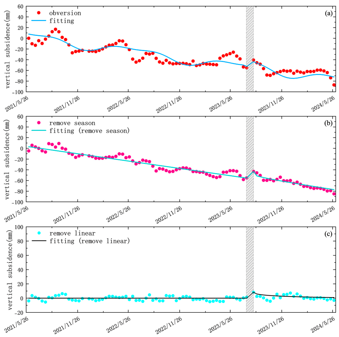
Prior to presenting the final spatial extraction results, we first analyzed the average deformation signal over the entire flood-inundated area to validate the fitting approach. We computed the mean deformation of all PS points within the inundated area, performed the fitting, and applied the signal extraction workflow described above. The signal separation results for the mean vertical InSAR time series are shown in Figure 5. In Figure 5a, red dots represent the observed vertical deformation time series, and the blue line shows the corresponding fitting curve. In Figure 5b, purple dots denote the deseasonalized time series, with the light blue line as its fit. In Figure 5c, cyan dots show the deseasonalized and detrended time series, and the black line represents the fitting result. The shaded band marks the period of intense rainfall associated with the “23·7” flood. The mean uplift over the flood-inundated area reaches approximately 10 mm.

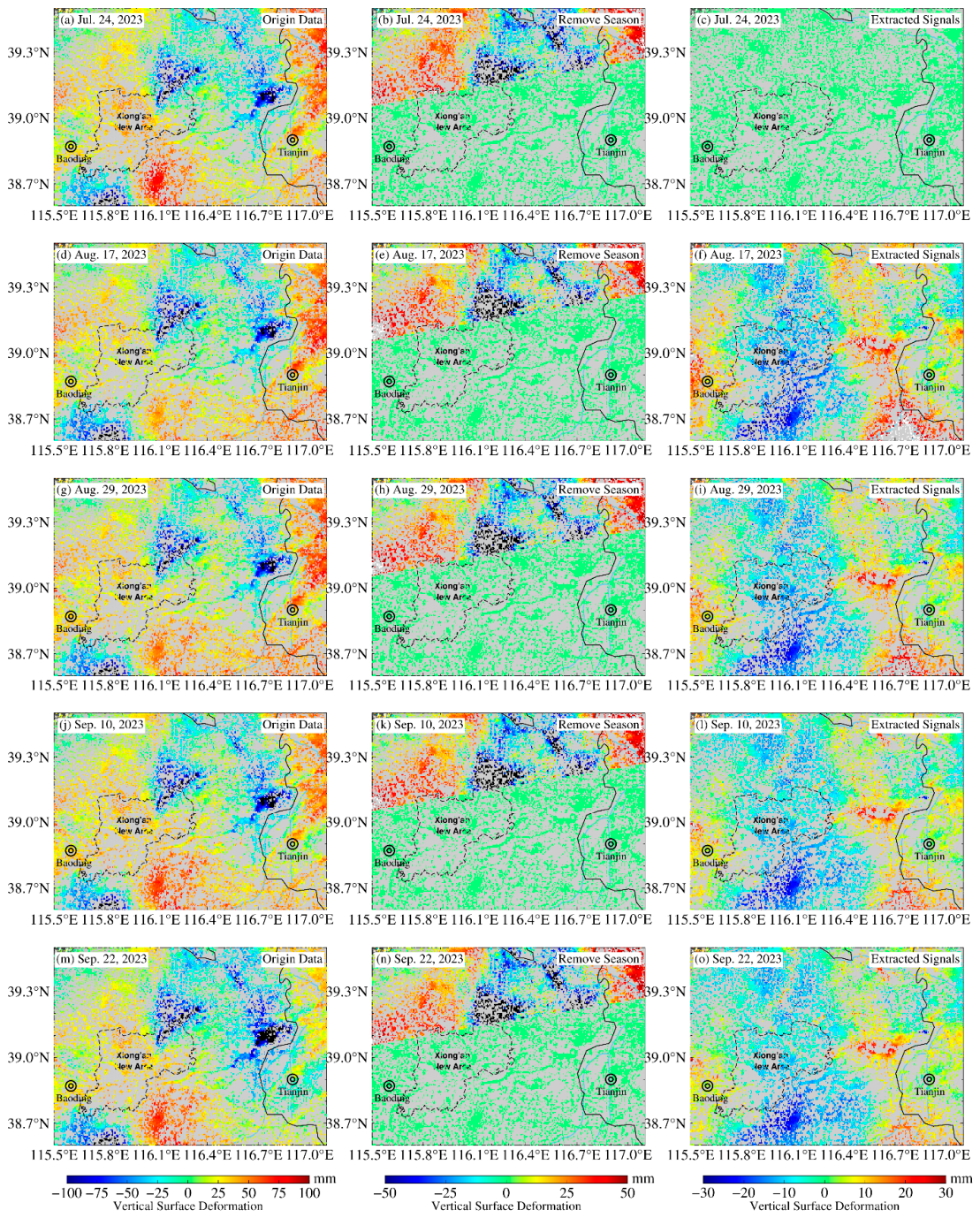
By applying the fitting procedure to every pixel, removing the linear trend, and normalizing the pre-flood baseline of each pixel to zero, we derived the spatial distribution of flood-associated surface deformation. The stepwise extraction results are shown in Figure 6. Figure 6 displays three sets of spatial maps: the original observed time series, the time series with periodic terms removed, and the final series after deseasonalization, detrending, and orbital error correction. As extraction proceeds, periodic signals, trend components, and orbital errors are progressively removed, and an uplift signal with a spatial pattern matching the flood extent becomes apparent east of Xiong’an New Area. However, due to specular reflection of the SAR signal off water surfaces, the flood-covered area southwestern Xiong’an New Area near Baiyangdian Lake exhibits large data gaps due to the absence of valid PS points. Notably, the spatially averaged InSAR signal in Figure 5 was used solely to verify that the observed flood-related deformation is consistent with the spatial results in Figure 6. The agreement in direction and magnitude between the averaged signal and pixel-level results confirms the validity of the extraction method at this stage.

Prominent diagonal striping is visible in Figure 6f–j. This arises because the SLC data for each date are mosaicked from two adjacent frames to ensure full coverage of the study area. In standard StaMPS processing, such orbital errors are removed by differencing all acquisitions relative to the initial reference image. Our fitting procedure shares similarities with the StaMPS workflow for generating mean annual deformation rates. The key difference is that StaMPS uses linear fitting to output annual deformation rates, whereas we use a more complex fitting function to model flood-related transient changes. As a result, orbital errors remain in the fitted time series, requiring an additional correction step. Furthermore, since this study focuses on flood-related deformation signals, all post-flood acquisitions are differenced relative to the last pre-flood acquisition. After removing periodic and trend components, we obtained the final flood-associated deformation signals, shown in Figure 6k–o.

The date of 24 July 2023, is the last pre-flood acquisition, and its cumulative deformation is set to zero as the reference baseline. In the four subsequent acquisitions, we observed deformation signals with a spatial pattern matching the flood extent in Bazhou, east of Xiong’an New Area. In areas far from the inundation zone, however, the extracted time series show notable overfitting artifacts. This issue stems from an inherent limitation of parametric fitting approaches [16,34]: in non-inundated regions, there is no genuine flood-induced transient deformation process that follows the step + logarithmic decay pattern. When the parametric fitting function is applied uniformly across the entire study domain, it inevitably maps high-frequency noise and random disturbances in these areas onto the prescribed step and logarithmic decay terms, misinterpreting noise as flood-related transient signals. Such sensitivity to high-frequency noise is a common drawback shared by most parametric time-series decomposition methods.

To quantitatively evaluate the severity of overfitting and its influence on our findings, we performed statistical analysis on all valid PS points outside the flood inundation boundary. The results indicate that the mean absolute value of the extracted “flood signal” in non-inundated areas is 2.7 mm, with a 95th percentile of 4.8 mm—one order of magnitude smaller than the 30 mm maximum uplift in the core inundation zone. Spatially, these artifacts present a random and discrete distribution, with no coherent spatial pattern matching the flood inundation extent. Since all core analyses of this study are concentrated on the well-defined W-shaped and 7-shaped core inundation zones with strong and reliable flood signals, the weak spurious signals in non-inundated areas do not compromise the validity of our core conclusions on deformation characteristics and the underlying physical mechanism.

To alleviate overfitting in future applications, we propose two feasible optimization directions. First, spatial constraints can be incorporated, such as mask-based fitting constrained by flood inundation extent, or neighborhood spatial regularization that penalizes transient signals inconsistent with adjacent pixels. Second, an L1-norm penalty term can be added to the fitting objective function to suppress noise-induced spurious step and logarithmic decay terms in noise-dominated pixels. It should be clarified that these optimizations will be further investigated in subsequent work, and they do not affect the core conclusions of the present study.

Importantly, the extraction results are not driven by the filtering step. Temporal filtering and flood signal extraction are two separate, independent procedures: the extraction step does not depend on the choice of filtering parameters. As shown in Figure 6, flood signals were extracted directly from the PS-InSAR time series using the three-stage composite fitting model (linear trend + step + logarithmic decay) from Equation (2), solved via nonlinear least squares. This model explicitly represents and separates each signal component, and its performance depends on how well the mathematical formulation captures the underlying physical processes, rather than on specific filtering parameter values.

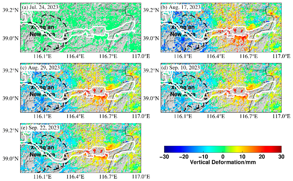
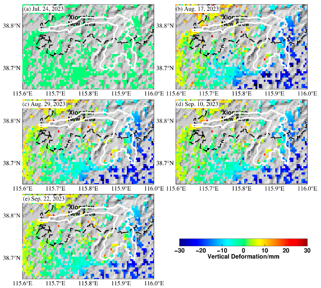
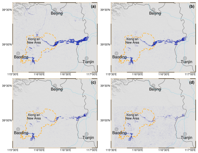
Flood data from Jiao et al. [58] indicate that two distinct inundation zones emerged after 17 August: a W-shaped zone east of Xiong’an New Area and a 7-shaped zone to the southwest. We extracted these two key sub-areas for detailed analysis, with results shown in Figure 7 and Figure 8. The extracted signals show the expected pattern of minimal pre-event variation and pronounced post-event change, confirming that flood-related deformation signals have been successfully separated. As shown in Figure 8, the 7-shaped inundation zone in southern Xiong’an New Area exhibits incoherent deformation patterns that are difficult to interpret directly. This is due to widespread but shallow water cover and specular reflection of SAR signals off the water surface. Data gaps in the center of the inundated area arise because specular reflection prevents the backscattered signal from being received; these pixels cannot be processed interferometrically in PS-InSAR, resulting in blank regions. As shown in Figure 1, the W-shaped inundation zone east of Xiong’an New Area features extensive inundation and greater water depth, which would be expected to produce a strong surface deformation response. Pronounced uplift is clearly visible in the areas surrounding this W-shaped zone, with a spatial pattern closely matching the shape of the inundation area. The deformation in this zone correlates well with the flood distribution, demonstrating that Equation (2) reliably represents the surface deformation associated with the “23·7” flood.

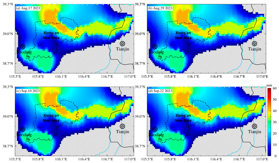
Since flood-inundated areas are primarily distributed along the river system, we clipped the InSAR time series to the flood-affected extent based on the loading simulation results. As shown in Figure 6, flood-related deformation in the core inundation area shows net uplift between 24 July and 17 August. To better visualize the uplift signal, we excluded pixels showing subsidence within the study area. The final spatial distribution results are presented in Figure 9.

Figure 9 demonstrates that zones of pronounced deformation gradually contracted and decayed in magnitude over time within the “23·7” flood inundation area. However, notable deformation persisted in the inundated zones for several months after the flood receded. Combined with the groundwater simulation results presented later, we attribute this to infiltrated floodwater that did not drain rapidly but instead remained in the shallow subsurface near the inundation zones for an extended period. The maps in Figure 9 start from 17 August 2023, to focus on the spatiotemporal evolution of flood-related deformation following the event.

To quantitatively evaluate the spatial consistency between the extracted deformation and flood inundation, we calculated the Intersection over Union (IoU) and Cohen’s kappa coefficient using the flood extent as reference. Defining significant uplift as deformation > 5 mm, the IoU between the uplift zone and inundation boundary reaches 0.78, with a kappa coefficient of 0.72 for the W-shaped eastern inundation zone. These metrics confirm strong spatial agreement between the extracted signal and the actual flood distribution.

3. Numerical Simulation of Land Subsidence Based on Loading Theory During the “23.7” Flood

3.1. Numerical Simulation of the Loading Effect

The “23·7” flood represents a classic surface loading problem, well suited for analysis using loading theory. We performed our loading calculations using LoadDef (v2019), an open-source toolkit developed by the University of Montana. This Python (v3.10)-based package computes elastic deformation induced by surface mass loading on a spherically symmetric Earth model [39]. LoadDef (v2019) adopts the Preliminary Reference Earth Model (PREM) [66] as its internal Earth structure, which provides all parameters required for loading deformation calculations—including Lamé parameters, density, P- and S-wave velocities, and gravitational acceleration for each layer—under the assumption of a layered, isotropic, rotating elastic Earth.

The LoadDef (v2019) workflow comprises three main steps: Love number computation, Green’s function derivation, and disk loading response calculation. Love numbers are dimensionless parameters that describe elastic deformation and gravitational perturbations of the Earth in response to external mass loading, including tidal forces and surface loads. They are grouped into three categories (gravitational potential, loading, and shear), each containing three coefficients corresponding to vertical displacement, horizontal displacement, and gravitational potential change.

Green’s functions provide a rigorous framework for solving linear partial differential equations governing deformation in geophysics and are particularly well suited for linear systems. The core principle is that the deformation produced by any complex load source can be derived by decomposing the source into infinitesimal point loads and integrating the corresponding Green’s functions. For tilt and strain Green’s functions, a disk factor is required to ensure near-field convergence [38]. This factor approximates a point load as a uniform load distributed over a small finite disk, which is valid when the disk radius is much smaller than the distance to the observation point.

LoadDef (v2019) supports Green’s function computation in three reference frames: CE—origin at the center of mass of the solid Earth; CM—origin at the center of mass of the entire Earth system; CF—origin at the center of figure of the solid Earth surface [42]. Since this study focuses on vertical surface displacement induced by flood loading, all subsequent loading calculations are performed in the CF reference frame.

The disk loading model represents a distributed surface load as a uniform-pressure disk of equal total mass. Although this is an idealization, it is mathematically tractable and provides a reasonable approximation for many real-world applications [39]. The “23·7” flood inundation covers two main zones with complex geometries, highly variable water depths, and strongly heterogeneous distribution [58]. To improve calculation realism, we discretized the flood load into a large number of small disks while preserving the total water mass. The discretization procedure was as follows: (1) We gridded the original flood data at its native 10 m × 10 m resolution. (2) For each grid cell, we defined an equivalent disk centered on the cell, with a diameter equal to the cell side length, converting each square prismatic water column into a cylindrical disk of equal volume. (3) We aligned observation points with the geographic coordinates of the PS-InSAR pixels to enable direct comparison. (4) We summed the Green’s function responses from all disks to obtain the total loading-induced deformation across the entire flood-inundated area.

After precomputing the Love numbers and Green’s functions, we imported the flood dataset to run the disk loading calculations. The calculation treats the flood as a collection of equal-radius cylindrical loads and sums their individual contributions at each observation point to produce the final subsidence field for the study area.

3.2. Flood Data Sources and Preprocessing

The flood inundation data used in this study were derived from the SAR-based analysis by Jiao et al. [58], generated from Sentinel-1A C-band Ground Range Detected (GRD) imagery. GRD is a Level 1 product of the Sentinel-1 mission, produced by multi-looking the corresponding Single Look Complex (SLC) data and projecting from slant range to ground range using the WGS84 ellipsoid.

GRD pixels contain amplitude information of the imaged scene, while phase information is discarded during processing. The product has approximately equal resolution in the azimuth and range directions, which reduces speckle noise but decreases geometric resolution relative to SLC data. Thermal noise is also removed in GRD products to improve image quality.

The flood data in this section are at 10 m resolution and correspond to ascending track A142. Since the “23·7” flood inundation covers only a small fraction of the Sentinel-1A swath, we manually cropped the dataset to the study area to balance computational accuracy and efficiency.

The dataset from Jiao et al. [58] includes five temporal snapshots: 5 August, 17 August, 29 August, 10 September, and 22 September 2023. The 5 August snapshot captures the early flood stage, with inundation concentrated primarily in Bazhou north of Xiong’an New Area [58]. However, the extreme rainfall event—compounded by the effects of Typhoon Doksuri, heavy cloud-induced diffuse scattering, and elevated atmospheric water vapor from flood evaporation—caused severe phase unwrapping errors and degraded accuracy in the 5 August SLC data. We therefore excluded the 5 August flood data from our analysis.

The remaining four water depth datasets are provided in GeoTIFF format at 10 m × 10 m resolution. To optimize memory usage, we first converted the GeoTIFF files to HDF5 format. HDF5 is designed for large-scale dataset storage and management, supports parallel I/O and multiple compression algorithms, and substantially reduces storage footprint, improves read/write speed, and lowers hardware requirements for data processing. We then converted the HDF5 files into chunked DAT files for more efficient batch reading and computation.The flood distribution (without water depth) obtained after the above processing is shown in Figure 10.

3.3. Flood Loading Effect Field Associated with the “23·7” Flood Event

To enable direct comparison between loading calculations and InSAR observations, we aligned the observation point locations with the PS-InSAR pixel coordinates. Since InSAR cannot resolve deformation signals below ~0.4 mm, we excluded pixels with predicted loading values below this threshold to reduce computational load and speed up calculations.

The theoretical loading-induced deformation results for the “23·7” flood are presented in Figure 11. Two prominent subsidence patterns are visible: a W-shaped zone east of Xiong’an New Area and a 7-shaped zone to the south. Loading-induced subsidence ranges from 0 to 2 mm across the main inundation area, and its spatial distribution closely matches the flood inundation extent and water depth distribution. As the flood receded, the magnitude of subsidence decreased progressively. By 22 September 2023, only the 7-shaped inundation zone in southern Xiong’an New Area retained measurable loading deformation.

To validate the proposed signal extraction method, we compared the extracted InSAR deformation field with both the flood inundation data and the theoretical loading results. The comparison is illustrated in Figure 12.

Spatially, the theoretical subsidence field is highly consistent with the flood inundation pattern, with maximum values in the core inundation zones and gradual attenuation with distance from the flooded area. Temporally, the areal extent of flooding decreased from 17 August onward, and the corresponding loading subsidence diminished accordingly. By 22 September, most floodwaters had receded, leaving only the 7-shaped southern inundation zone still submerged.

4. Numerical Simulation of Pore Water Rebound Effect Based on the Principle of Effective Stress

4.1. Numerical Simulation Method for Pore Water Rebound Effect Based on the Principle of Effective Stress

In this section, we combine numerically simulated groundwater level changes with forward modeling based on the effective stress principle and the quantitative relationship between water level fluctuations and surface deformation established by Poland [51] to compute the magnitude of flood-related surface uplift for the “23·7” event. The pore water rebound effect in the alluvial sediments of the North China Plain following flood recharge is quantified using the spatial distribution of groundwater level changes output by GMS.

The effective stress principle states that the total overburden stress from overlying sedimentary layers and surface loads is supported jointly by the effective stress of the aquifer skeleton and pore water pressure. At equilibrium, the relationship is as follows [63]:

$$p=p_{s0}+p_{w0}$$

(5)

where $p$ is the geostatic pressure, $p_{s0}$ is the initial effective stress of the soil skeleton, and $p_{w0}$ is the initial pore fluid pressure. Poland [51] noted that for unconfined aquifers, the ratio of effective stress to pore pressure change is approximately 3:2, and for confined aquifers approximately 3:1.

Total overburden stress remains constant over short timescales. A rise in groundwater level increases pore water pressure, which reduces effective stress on the aquifer skeleton and causes the formation to expand and rebound until a new equilibrium is reached. The unit weight of water is 10 kPa/m, meaning each meter of water level change corresponds to a 10 kPa change in pore pressure [51]. For a groundwater level change $\mathsf{\Delta }h$, the updated pore water pressure $p_w$ and the resulting change in effective stress ${\mathsf{\Delta }p}_s$ are

$$p_w=10·∆h+p_{w0}$$

(6)

$$∆p_s=p-p_w$$

(7)

Substituting Equation (5) gives the relationship between effective stress change and water level change:

$$∆p_s=p-p_{w0}-10·∆h-p_{s0}$$

(8)

The resulting change in formation thickness $\mathsf{\Delta }b$ is a function of the volume compressibility $M_v$, initial formation thickness $b_0$, and a scaling factor $s$:

$$∆b=s·∆p_s·M_v·b_0$$

(9)

where the coefficient of volume compressibility $M_v$ is calculated from the initial porosity $n_0$, initial void ratio $e_0$, new void ratio $e$, compression index $C_c$, initial effective stress $p_{s0}$, new effective stress $p_s$, and coefficient of compressibility $a_v$. The calculations for these parameters are as follows, and the selection of some parameters needs to be based on the characteristics of regional rock strata [63]:

$$e_0={\displaystyle \frac{n_0}{1-n_0}}$$

(10)

$$e=e_0-c_c·\mathit{log}\left({\displaystyle \frac{p_s}{p_{s0}}}\right)$$

(11)

$$M_v={\displaystyle \frac{a_v}{1+e_0}}$$

(12)

$$a_v={\displaystyle \frac{e_0-e}{∆p_s}}$$

(13)

Based on the above, the quantitative relationship between the surface deformation $\mathsf{\Delta }b$ and the groundwater level change $\mathsf{\Delta }h$ is mediated by the change in effective stress ${\mathsf{\Delta }p}_s$; thus, we can derive the required forward calculation equation:

$$∆b=M_v{b}_o\left(p-p_{s0}-p_{w0}-10·s·∆h\right)$$

(14)

where $s$ is the scale factor used to account for and predict inelastic deformation. The value of this parameter is obtained as follows: first, calculate the measured water level change rate based on well data, and set $s=1$ (assuming perfectly elastic deformation) to calculate the theoretical surface uplift rate using the following formula:

$$v_m=s·M_v·b_0·{\rho }_w·g·{\displaystyle \frac{∆h}{∆t}}$$

(15)

where ${\rho }_w$ is the density of water, $g$ is the gravitational acceleration, and $v_m$ is the theoretical surface uplift rate.

Subsequently, we extracted the InSAR deformation rate results within a 1 km radius around each well. Considering local noise and outliers, the 95th percentile was adopted as the observed surface uplift rate. For each borehole, we calculated the $s$ value that minimizes the root mean square error (RMSE) between the theoretical velocity and the observed velocity. Finally, we averaged the $s$ values obtained from all wells as the scale factor for the study area. The calculation formula for s is as follows:

$$s=\underset{s}{\mathit{min}}\sqrt{{\displaystyle \frac{1}{n}}\sum {\left(v_m-v_{InSAR}\right)}^2}$$

(16)

where $v_{InSAR}$ is the observed surface uplift rate.

The forward calculation of surface uplift deformation based on the groundwater level change data obtained from numerical simulation mainly includes the following steps.

• Determination of initial state: Extract grid-wise groundwater level changes $\mathsf{\Delta }h$ from GMS outputs. Set initial aquifer thickness ($b_0$ = 200 m) based on borehole data [62], and assign initial porosity $n_0$ and compression index $C_c$ according to the lithology of the North China Plain alluvial sediments.
• Geomechanical parameter calculation: Calculate the initial void ratio $e_0$ of the stratum based on the initial porosity $n_0$, then derive the coefficient of volume compressibility $M_v$ using the compression index $C_c$ determined in the previous step, and convert it into the change in effective stress.
• Scale factor calculation: Use the extracted InSAR deformation as validation data. Compute RMSE between modeled and observed uplift within 1 km of each borehole, and iteratively optimize s to minimize RMSE.
• Forward calculation: Apply the calibrated scale factor across the entire study area, substitute all parameters into Equation (15), and generate the final surface deformation field driven by pore water rebound.

4.2. Numerical Simulation of Groundwater Level Change

Flood-related surface deformation is not driven solely by surface water loading. The North China Plain is a typical alluvial plain with high sediment porosity, and pore water rebound effects can be substantial. Our InSAR signal extraction results are consistent with the hypothesis that pore water rebound dominates over loading effects. In this section, we use GMS (Groundwater Modeling System) v10.8 to quantitatively simulate the spatiotemporal pattern of groundwater level changes during the “23·7” flood, constrained by borehole data, watershed boundaries, flood inundation maps, hydrological records, and precipitation data.

The groundwater flow model is built on several simplifying assumptions to ensure computational feasibility and representativeness: the aquifer system is homogeneous and isotropic within each layer, with hydraulic properties assigned based on field measurements and literature values; lateral boundary conditions are fixed across the model domain; and recharge rates, hydraulic conductivity, and storage parameters are held constant within each stress period.

We simulate three-dimensional transient groundwater flow via the finite difference method, governed by the seepage equation derived from Darcy’s law and mass conservation:

$${\displaystyle \frac{\partial }{\partial x}}\left(K_{x}h{\displaystyle \frac{\partial h}{\partial x}}\right)+{\displaystyle \frac{\partial }{\partial y}}\left(K_{y}h{\displaystyle \frac{\partial h}{\partial y}}\right)+{\displaystyle \frac{\partial }{\partial z}}\left(K_{z}h{\displaystyle \frac{\partial h}{\partial z}}\right)-w=Sy{\displaystyle \frac{\partial h}{\partial t}}$$

(17)

This equation describes the transient process of three-dimensional groundwater flow and is based on Darcy’s Law and the continuity equation [34], where $K_x,K_y \mathrm{a}\mathrm{n}\mathrm{d} K_z$ are the hydraulic conductivities in each direction ($\mathrm{m}/\mathrm{d}\mathrm{a}\mathrm{y}$), h is the groundwater head ($\mathrm{m}$), w is the volumetric flux per unit volume $({\mathrm{m}}^3/\mathrm{d}\mathrm{a}\mathrm{y})$, $t$ is time $\left(\mathrm{d}\mathrm{a}\mathrm{y}\right)$, and $S_y$ is the specific yield of the porous medium, which is dimensionless. This method enables the model to effectively simulate the spatiotemporal dynamics of groundwater. The groundwater simulation in the GMS v10.8 mainly includes the following steps.

• Conceptual model construction and grid discretization: The model domain covers the main flood-inundated areas and surroundings. We import a Digital Elevation Model (DEM) to represent surface topography and construct a 3D geological model using watershed boundaries and borehole data. Strata are generalized into hydrogeological units (e.g., shallow sand layers, clay aquitards, deep gravel layers) and discretized into a fine 3D finite-difference grid with ~1 km × 1 km horizontal resolution. Borehole data are sourced from the Baiyangdian watershed hydrogeological report by Zhang et al. [61].
• Boundary conditions and source/sink terms: Watershed boundaries and flood inundation zones define the main model constraints. We designate the 17 August 2023 flood inundation extent from Jiao et al. [58] as the primary groundwater recharge zone. Recharge rates are estimated from precipitation and surface water infiltration properties and applied as time-varying dynamic boundary conditions. Precipitation data are from the China Meteorological Administration (CMA), and infiltration parameters are taken from the Baiyangdian hydrogeological report [61].
• Parameter assignment and steady-state calibration: The basic parameters assigned to the model include hydraulic conductivity ($K$), specific storage ($S_s$), and specific yield ($S_y$), among others. We first run a steady-state simulation to reproduce the pre-flood equilibrium flow field. The model is then automatically calibrated against measured well water levels using the PEST parameter estimation tool by adjusting hydraulic conductivity and recharge rates to minimize head residuals. Observed well data are from Long et al. [62].
• Transient simulation: Using the calibrated steady-state flow field as the initial condition, we run a transient simulation covering the flood event and post-flood period. Outputs include grid-wise groundwater level changes ($\mathsf{\Delta }h$) at selected time steps, which provide input for subsequent pore water rebound calculations.

The intense rainfall phase of the “23·7” flood occurred from 27 July to 2 August 2023. For computational simplicity, we aggregate total event rainfall into early August. To enable direct comparison with InSAR results, we align the transient simulation output dates with Sentinel-1A acquisition times: 17, 29, 41, and 53 days after the early August recharge event. We do not extend the simulation further because the total flood duration is ~65 days [58], and the designated recharge zones are no longer representative after flood recession.

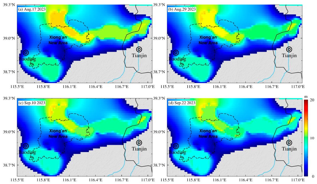
The overall simulation period spans 1 July to 31 August 2023, with focus on dates matching Sentinel-1A overpasses. The spatial distribution of maximum groundwater level rise is shown in Figure 13.

Simulation results show that the spatial pattern of groundwater level changes closely matches the actual flood extent. Two distinct zones of water level rise are evident: the W-shaped inundation area in the Daqing River basin east of Xiong’an New Area, and the 7-shaped area southwest of Xiong’an near Baiyangdian Lake.

Consistent with the alluvial plain hydrogeology of the North China Plain, infiltration of precipitation and floodwater into the shallow aquifer is substantial, and aquifer permeability is relatively high. Local maximum groundwater level rise reaches 16 m, and water level changes in non-core areas decrease gradually outward from the two inundation zones. Furthermore, as surface ponding recedes, groundwater does not drain rapidly laterally but remains stored near the inundation zones, with drainage timescales longer than the surface flood recession period.

An important modeling assumption must be noted: we use the 17 August flood extent as the primary recharge constraint for the groundwater model. This choice is driven by the InSAR observation constraint: the W-shaped uplift signal east of Xiong’an corresponds to the main inundation pattern after 17 August. According to 5 August flood data [58], substantial floodwater was still located in Zhuozhou, north of Xiong’an New Area, on that date. However, the 5 August SLC images are severely degraded by atmospheric water vapor and cloud cover, causing major phase unwrapping errors and reducing PS-InSAR data quality. We therefore exclude the 5 August SLC data from our analysis.

As a consequence, neither the flood dataset nor the groundwater simulation can account for the 5 August inundation pattern, and groundwater distribution cannot be constrained by that date’s flood extent. This leads to an overestimation of floodwater and groundwater retention in northern Xiong’an New Area and Xiong County, as floodwater that was actually in Zhuozhou is effectively assigned to the southern area. Importantly, this limitation has minimal impact on the W-shaped eastern inundation zone, where the flood spatial pattern is fully consistent with observations, and results there remain reliable.

The three-dimensional transient groundwater flow model is built based on the 1:50,000 hydrogeological survey data of the Baiyangdian Basin, with a standardized three-layer hydrogeological conceptual model generalized from field borehole records. From top to bottom, the subsurface stratigraphy consists of (1) surficial silty clay aquitard (0–10 m); (2) shallow sandy unconfined aquifer (10–120 m), the primary stratum receiving rapid flood infiltration recharge; and (3) deep continuous clay aquitard below 120 m, which is set as the bottom no-flow boundary of the model.

It should be clearly stated that transient electromagnetic (TEM) geophysical detection data are not adopted to constrain subsurface stratigraphic geometry in this work; all stratigraphic thickness and lithology information entirely comes from standardized borehole logging profiles of the Baiyangdian regional hydrogeological report. To quantitatively verify the robustness of modeling results, we conduct a parameter sensitivity analysis targeting hydraulic conductivity and infiltration recharge coefficients. Within reasonable parameter perturbation ranges (±30% for hydraulic conductivity, ±20% for recharge coefficient), the simulated maximum 16 m groundwater rise and peak 36 mm pore water rebound uplift only fluctuate within ±10%, which confirms the stability of our forward simulation outputs. We acknowledge that stratigraphic simplification based on limited borehole data may introduce minor modeling uncertainties, and we will collect more full-domain geological exploration data to refine layered structures and narrow the deviation between simulated and real groundwater dynamics in follow-up research.

4.3. Surface Deformation Field of Pore Water Rebound Effect Associated with the “23·7” Flood Event

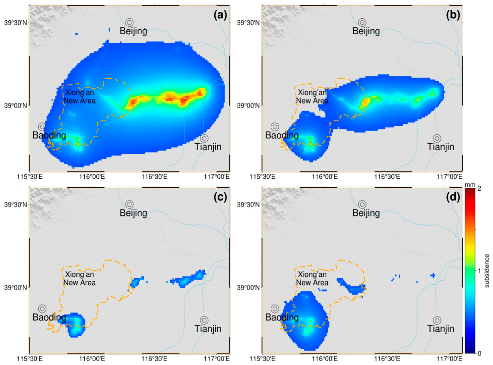
Using the simulated groundwater level changes described above, we computed surface uplift from pore water rebound via the effective stress–surface deformation relationship established by Poland [51]. Results are presented in Figure 14. Widespread surface uplift occurred across the study area during the “23·7” flood. The spatial pattern of uplift magnitude is strongly correlated with the amplitude of groundwater level rise and also agrees well with the loading-theory subsidence field, flood inundation extent, and InSAR-extracted deformation. The largest uplift values are concentrated in the W-shaped Daqing River inundation zone east of Xiong’an New Area and the 7-shaped zone southwest of Xiong’an near Baiyangdian Lake. The maximum uplift in the W-shaped zone reaches 36 mm, which is consistent in order of magnitude with the InSAR observation of 30 mm.

We note that the forward-modeled pore water rebound produces anomalously strong signals in Xiong County (northeastern Xiong’an New Area), an artifact of model simplifications. As a result, modeled uplift in Zhuozhou (northern Xiong’an) and Xiong County deviates from the InSAR-extracted signals. By contrast, the W-shaped eastern inundation zone shows highly consistent spatial patterns and deformation magnitudes between model and observations.

Within the W-shaped zone, pore water rebound from groundwater level rise produces a maximum uplift of 36 mm, while surface water loading produces a maximum subsidence of 2 mm. The net effect of these two processes agrees well with the 30 mm maximum uplift extracted from InSAR, in both magnitude and sign. This confirms that flood-related surface deformation is not a simple loading problem but arises from the combined action of pore water rebound and spherical elastic loading. Among these two mechanisms, pore water rebound driven by rapid groundwater recharge is clearly dominant.

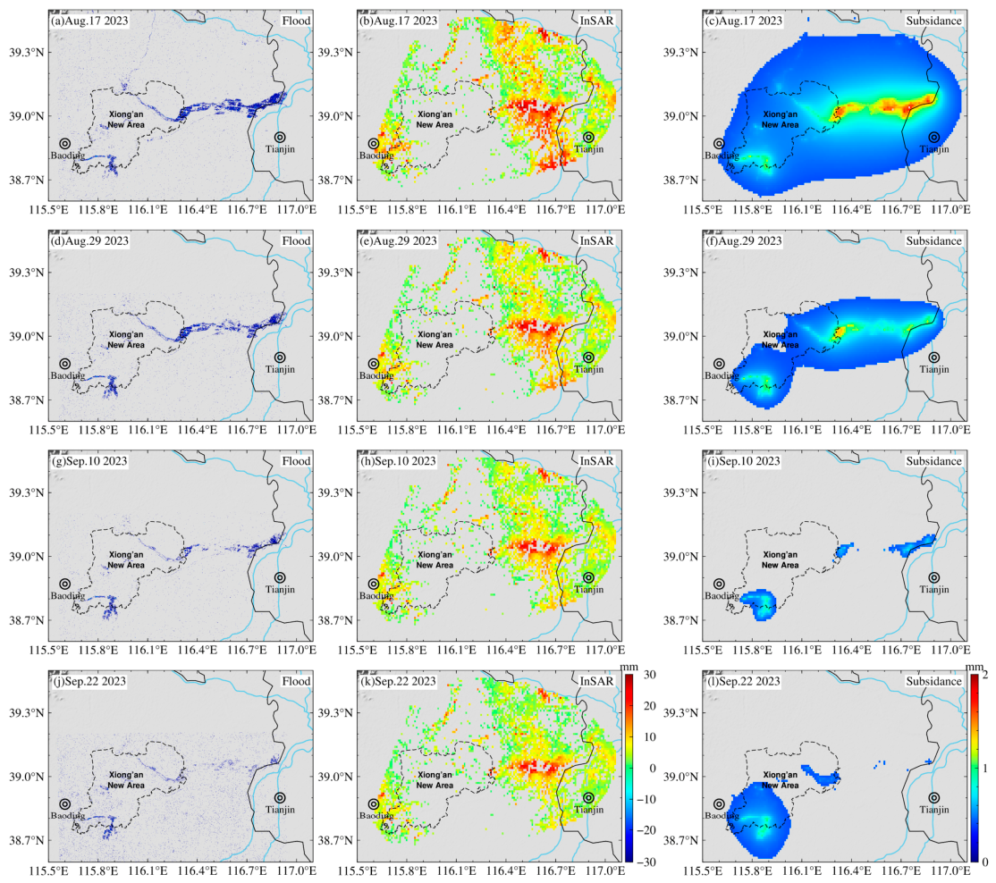
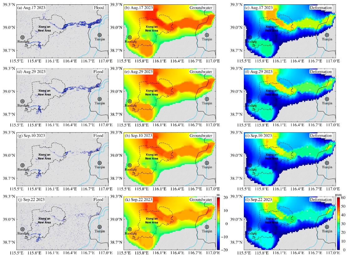
To further examine the physical mechanism, we compared flood inundation patterns, groundwater level changes, and pore water rebound forward results side by side (Figure 15). All three datasets show high spatial consistency: zones of strong groundwater level rise correspond closely to core inundation areas (particularly the eastern W-shaped and southwestern 7-shaped zones), and the resulting pore water rebound uplift is concentrated in the same locations. When the 36 mm maximum rebound uplift is combined with the 2 mm maximum loading subsidence, the net deformation matches the InSAR-observed maximum uplift of 30 mm in both magnitude and vertical direction. This comparison strongly supports the conclusion that InSAR-observed deformation results from the combined action of pore water rebound and surface water loading, with the rebound mechanism being overwhelmingly dominant. The good agreement between observation and model also validates that the proposed signal extraction method reliably separates flood-related surface deformation from background signals.

To quantify the agreement between InSAR observations and forward modeling results, we sampled 1200 valid PS points within the W-shaped inundation zone and computed statistical metrics. The Pearson correlation coefficient between observed uplift and modeled combined deformation is 0.81, with a mean absolute error (MAE) of 3.2 mm and RMSE of 4.1 mm. Given that InSAR observations contain residual atmospheric noise and the model involves hydrogeological parameter simplification, this level of agreement provides robust quantitative support for the pore water rebound dominance mechanism.

4.4. Formation Mechanism of Surface Deformation Associated with the “23·7” Flood Event

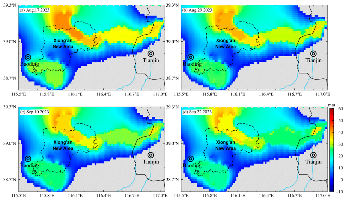
Finally, we combined the loading-theory and pore water rebound forward results into a total deformation field (Figure 16) and compared it with the InSAR-extracted signals.

In the W-shaped inundation zone east of Xiong’an New Area, both the forward-modeled and observed deformation signals are well defined and consistent in sign and magnitude. However, specular reflection of SAR signals off open water surfaces redirects energy away from the sensor, causing widespread data gaps over the core inundation zones and reducing point coverage in the most flood-affected areas.

The forward model also produces anomalously strong deformation responses in Xiong County (northeastern Xiong’an) and Zhuozhou (immediately north of Xiong’an), with magnitudes larger than those in the core inundation zones. This discrepancy arises primarily because the modeled flood recharge extent does not match the actual early-stage flood distribution. Inspection of the flood data from Jiao et al. [58] shows that on 5 August 2023, the main inundation was concentrated along the Baigou River, differing from the 17 August pattern used as model input. Because the 5 August InSAR data are of insufficient quality, we did not include this time step in the analysis, which causes the northern Xiong’an simulation and forward results to deviate from observations.

Additionally, noticeable boundary effects appear in western Tianjin, caused by the limited lateral extent of the groundwater model domain. We acknowledge that multiple simplifications were applied in the numerical simulations.

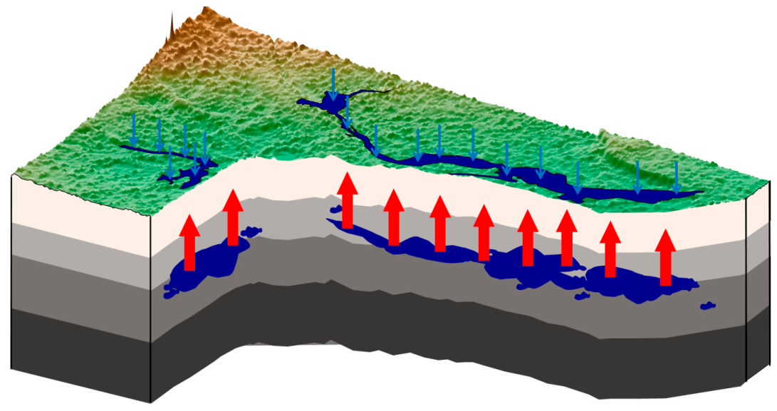
Despite these limitations, the high agreement between simulated and observed deformation in the core inundation zones—in spatial pattern, sign, and magnitude—confirms the validity and reliability of the proposed method. The “23·7” flood-related surface deformation is dominated by uplift and arises from the combined action of pore water rebound and flood loading, with the rebound mechanism being dominant. The conceptual mechanism is illustrated in Figure 17: blue arrows indicate subsidence caused by floodwater loading, and red arrows indicate surface uplift driven by pore water rebound associated with rising groundwater levels.

5. Discussion

In Chapter 2, we presented an InSAR time-series analysis method based on a three-stage composite fitting model and successfully isolated surface deformation signals associated with the “23·7” extreme Haihe River flood from Sentinel-1A data. In Section 3 and Section 4, we compared forward simulations of spherical elastic loading and pore water rebound and showed that the observed flood-related uplift is dominated by pore water rebound driven by rapid groundwater recharge, whereas the conventionally expected surface water loading contributes only ~2 mm of subsidence.

These findings extend the application potential of InSAR for monitoring short-period hydrological events and provide quantitative evidence for the hydro-geomechanical coupling mechanism of floods in alluvial plains. Nevertheless, several limitations and uncertainties remain regarding signal extraction, model assumptions, and numerical simulations, which are discussed below alongside comparisons with previous studies.

5.1. Reliability and Limitations of InSAR Signal Extraction

Spatially, the extracted deformation signals agree well with the flood inundation extent [58], with a maximum uplift of ~30 mm observed in the W-shaped inundation zone east of Xiong’an New Area. This finding runs counter to the conventional expectation of flood-loading subsidence but matches the 36 mm uplift from our pore water rebound forward modeling in both magnitude and temporal trend. Nevertheless, the signal extraction approach has several sources of error and limitation.

First, the results are constrained by the 12-day revisit period of Sentinel-1A, which prevents full characterization of the detailed temporal evolution of flood-related deformation. Furthermore, the 5 August 2023, data were excluded due to poor phase unwrapping quality, resulting in additional loss of temporal detail. This gap means that the peak deformation and sub-monthly dynamics cannot be fully resolved using only Sentinel-1A observations.

Second, specular reflection of SAR signals from open water causes extensive data gaps over the core inundation zones. This is a well-known limitation of InSAR flood monitoring. In this study, deformation in the core inundated areas is inferred from surrounding non-inundated pixels, rather than measured directly. This indirect estimation may lead to underestimation of the maximum uplift or introduce spatial interpolation biases.

The overfitting artifacts in non-inundated areas represent a known limitation of parametric function fitting when applied to pixels without a true transient signal. As quantified in Section 2.4, the magnitude of these artifacts is small and spatially random, and they do not compromise the interpretation of deformation within the flood inundation zone.

We acknowledge the lack of direct independent ground truth as a critical limitation of this case study. We fully recognize that cross-validation using concurrent L-band or X-band SAR data and in situ GNSS measurements within inundated zones would greatly enhance the credibility of detected transient deformation signals. Unfortunately, no synchronous multi-band SAR datasets cover this flood event, and merely two GNSS stations are available in the whole study area, both far from core flood inundation zones without effective in situ displacement observations inside flooded regions. In addition, regional groundwater wells only supply monthly water level time series, whose low temporal resolution cannot match the 65-day short flood evolution process and thus cannot be treated as precise groundwater ground truth. Under such severe data constraints, the groundwater numerical simulation constrained by multi-source hydrological, borehole and flood inundation data is adopted as a compromised auxiliary verification scheme. To further validate the robustness and generalization of our method, we plan to apply the proposed extraction workflow to other alluvial plain flood cases for cross-case validation in our future research and integrate multi-source satellite and ground sensor data to comprehensively analyze flood-related surface deformation.

5.2. Rationality and Simplification of the Fitting Model Assumptions

The three-stage model (linear trend + step + logarithmic decay) provides a good fit to the observed time series and successfully isolates flood-related transient deformation. Nonetheless, it represents an idealized simplification of the actual physical processes, with three key caveats:

First, the extreme rainfall event lasted ~7 days (27 July to 2 August 2023). During this period, loading, infiltration, surface runoff, and evaporation operate simultaneously, rather than occurring as a sequential buildup-then-decay process. Second, flood recession is controlled by a combination of local topography, soil permeability, and drainage infrastructure, meaning real-world deformation does not follow a perfect logarithmic decay pattern.

Third, the model assumes pre-flood deformation follows a strictly linear trend and periodic signals follow a pure sine-cosine combination. In reality, domestic and industrial water use exhibits periodicity but also non-stationary variability, and high-frequency noise from irregular construction activities is also present in the time series. These factors can reduce the accuracy of the fitted background trend and seasonal terms.

Despite these simplifications, the model reliably extracts deformation signals whose spatial pattern closely matches the flood extent, even without prior hydrological constraints. This demonstrates that the method robustly captures the dominant target signal and that the results are not an artifact of mathematical manipulation or overfitting.

5.3. Comparison with Existing Research Results and Implications

Our results show that flood-related deformation arises from the combined action of pore water rebound and surface loading, with rebound being the dominant mechanism. This conclusion is consistent with analogous studies worldwide. The underlying geomechanical principle is that alluvial plain sediments have relatively high permeability, such that groundwater level rise from precipitation recharge often produces a pore rebound effect that outweighs the transient surface loading signal.

Chaussard et al. [53] reported ~20 mm of seasonal uplift in Mexico City driven by rainy-season groundwater recharge. Galloway et al. [52] documented uplift of similar magnitude in California’s Central Valley following rapid groundwater level recovery. Together, these studies establish that pore water rebound from groundwater recharge is a key control on seasonal surface deformation in alluvial plains. Our work aligns with this consensus and extends the mechanism from seasonal timescales to the short duration of an extreme flood event.

Chen et al. [54] used GRACE and InSAR to invert groundwater storage changes in the North China Plain, showing that widespread groundwater extraction causes significant land subsidence, but seasonal recharge can produce localized uplift. Yang et al. [18] similarly observed a correlation between seasonal deformation and groundwater levels in a PS-InSAR study of the Taiyuan region. For the “23·7” Haihe flood event, we go further by quantitatively disentangling the separate contributions of loading-induced subsidence and rebound-driven uplift via forward modeling, confirming the dominant role of pore water rebound for this event.

The finding that flood-related deformation is dominated by pore water rebound rather than loading-induced subsidence aligns with well-documented hydrogeological characteristics of alluvial plain aquifers worldwide. Previous studies have demonstrated that rapid groundwater recharge from intensive precipitation can generate measurable surface uplift that outweighs transient surface loading signals in high-porosity alluvial settings [52,53,60]. For the North China Plain specifically, prior work has shown that seasonal groundwater recovery can partially or fully offset long-term subsidence induced by groundwater extraction [18,54,65]. This study extends this established mechanism from seasonal timescales to the context of an extreme short-duration flood event, providing the first quantitative validation of pore water rebound dominance during a basin-wide extreme flood using InSAR observations and coupled forward modeling.

Parametric time-series decomposition models combining linear drift, annual/semi-annual sinusoidal seasonal terms, step offsets and logarithmic post-event decay have been widely utilized for seasonal aquifer deformation and postseismic signal extraction in previous geodetic research. Nevertheless, conventional one-step global parametric fitting tends to generate severe overfitting noise in pixels far from floodplains when processing short-duration flood signals with limited SAR observation samples. This study develops a stepwise iterative decoupling fitting pipeline, which eliminates seasonal oscillations and long-term linear background deformation sequentially before solving transient flood-related signals, greatly reducing spurious false deformation artifacts in non-inundated regions.

5.4. Contributions of This Study to Flood Disaster Risk Management and Its Prospective Application Potential

Although this work is based on retrospective observational data, the physical mechanisms identified have direct implications for flood risk management. The finding that alluvial plain flood deformation is dominated by pore water rebound uplift challenges the conventional “flood loading → foundation subsidence” assumption that underpins many existing foundation risk assessment frameworks, which may therefore contain systematic biases.

Furthermore, deformation signals persist for several months after flood recession, implying that geological hazards do not dissipate immediately as floodwaters recede. Sustained elevated pore water pressure can trigger secondary effects such as differential foundation settlement, and our results provide observational evidence for defining an appropriate monitoring window for post-flood secondary geohazards.

From a methodological perspective, the three-stage fitting framework requires only ~2 years of background InSAR time series as a baseline and can deliver near-real-time deformation estimates within ~12 days of a flood event. This makes it readily transferable to other river basins. When combined with real-time groundwater level monitoring, the forward modeling framework developed here can be further extended into a predictive tool, enabling a shift from post-event analysis to dynamic disaster risk assessment and providing geodetic observation support for regional disaster prevention and early warning.

The 12-day revisit cycle of Sentinel-1 enables near-real-time deformation monitoring within two weeks of a flood event, which is consistent with the operational timeline demonstrated in recent flood emergency remote sensing studies [27,30]. When integrated with real-time hydrological observations, the proposed fitting framework can support dynamic post-flood geohazard assessment, complementing conventional flood inundation mapping that focuses solely on surface water extent.

6. Conclusions

This study, focused on short-period extreme hydrological events such as floods, presents a model-fitting approach for InSAR time-series analysis and deformation signal extraction, and applies it to the basin-wide extreme “23·7” flood event in the Haihe River Basin. By combining spherical loading theory computations with forward simulations of groundwater pore water rebound, this study elucidates the spatiotemporal evolution and underlying physical mechanisms of flood-induced surface deformation. The main conclusions are summarized as follows:

(1)

To account for the rapid onset and short duration of flood events, we developed a surface deformation fitting function comprising a linear trend term, a step term, and a logarithmic decay term. This method effectively mitigates high-frequency noise that cannot be fully removed by conventional spatiotemporal filtering and successfully isolates transient and nonlinearly decaying deformation signals closely linked to flood evolution from complex InSAR time series.

(2)

The time-series surface deformation field of the “23·7” flood, extracted using the proposed method, reveals that inundated areas do not exhibit the expected subsidence during the event; instead, they show pronounced widespread surface uplift, with a maximum value of ~30 mm. The extracted deformation field closely matches the flood inundation extent spatially and follows a logarithmic-like decay pattern over time as the flood recedes. This consistency provides observational validation of the effectiveness and robustness of the proposed signal extraction method.

(3)

Multi-physics forward modeling shows that the surface water loading effect produces only ~2 mm of subsidence, whereas the pore water rebound effect—driven by substantial groundwater level rise from flood infiltration—generates up to 36 mm of surface uplift. The net combined deformation from the two mechanisms agrees closely with InSAR observations in spatial pattern, sign, and magnitude. This confirms that the prominent surface uplift across the inundated area is dominated by the pore water rebound effect, and represents a hydro-geomechanical coupling response rather than the purely loading-induced subsidence assumed in conventional understanding.

This study offers a novel technical framework for monitoring extreme hydrological events using geodetic techniques and delivers critical high-precision observational constraints and theoretical insights for advancing understanding of surface water–groundwater interactions and their associated complex surface deformation in alluvial plains. It also provides a robust observational basis for regional disaster prevention and emergency early warning efforts.