Article

Spatiotemporal Evolution and Multi-Factor Driving Mechanism of Land Subsidence in Shanghai Hongqiao Transport Hub Core Area Based on SBAS-InSAR (2015–2024)


1
School of Remote Sensing & Geomatics Engineering, Nanjing University of Information Science & Technology, Nanjing 210044, China
2
Technology Innovation Center for Integration Applications in Remote Sensing and Navigation, Ministry of Natural Resources, Nanjing 210044, China
*
Author to whom correspondence should be addressed.
Remote Sens. 2026, 18(17), 2848; https://doi.org/10.3390/rs18172848
Submission received: 8 July 2026 / Revised: 19 August 2026 / Accepted: 20 August 2026 / Published: 22 August 2026

Highlights

What are the main findings?
  • Urban functional zones and construction stages have surpassed geological factors as the dominant subsidence drivers in the Hongqiao Transport Hub, with their interaction exerting a bi-factor enhancement effect.
  • Two out-of-phase seasonal deformation signals are distinguished: near-instantaneous precipitation-driven surface loading on shallow soft soil and temperature-driven thermoelastic expansion of built structures, with distinct spatial distributions reflecting different urban surface conditions.
What are the implications of the main findings?
  • The GMM-derived deformation zoning map may provide a mechanism-informed tool for differentiated subsidence risk management in high-intensity urban development areas.
  • The integrated “GeoDetector–GMM–SSA” framework offers a transferable workflow for disentangling multi-factor coupling and seasonal deformation mechanisms in other soft-soil urban areas.

Abstract

Land subsidence in soft-soil urban transport hubs arises from the complex coupling of natural geology and intensive anthropogenic activities, yet its spatial differentiation mechanisms and seasonal drivers remain poorly understood in high-development core areas. This study develops a progressive analytical framework integrating Small Baseline Subset Interferometric Synthetic Aperture Radar (SBAS-InSAR), GeoDetector, Gaussian Mixture Model (GMM), and Singular Spectrum Analysis (SSA) to investigate spatiotemporal deformation patterns and driving mechanisms in the Shanghai Hongqiao Transport Hub Core Area from 2015 to 2024 using 209 Sentinel-1A images. Validation against official subsidence contours yields a Pearson correlation coefficient of 0.697 (p < 0.001) and an RMSE of 4.23 mm, confirming good spatial pattern agreement. Urban functional zones and construction stages are identified as the dominant influencing factors, with their interaction exhibiting notable bi-factor enhancement. Six distinct deformation response types are delineated via GMM, and two opposing seasonal signals are distinguished: near-instantaneous precipitation-driven surface loading on shallow soft soil and temperature-driven thermoelastic expansion of built structures. These findings may inform differentiated subsidence management and offer a transferable workflow for analogous soft-soil urban areas.

1. Introduction

Shanghai is located at the leading edge of the Yangtze River Delta, where Quaternary unconsolidated deposits exceed 200 m in thickness. The highly compressible, low-bearing-capacity soft clay makes it one of the most typical land-subsidence cities in China [1,2]. Cumulative subsidence in the central urban area has approached two meters [3]. Since 2006, Shanghai has implemented groundwater extraction restrictions, artificial recharge, and engineering-induced subsidence control, effectively containing large-scale regional subsidence [4,5]. However, urban development, underground space construction, and high-rise building loading still induce complex local deformation [6]. Situated in western Shanghai, the Hongqiao Transport Hub Core Area features compound land use and diversified engineering disturbances, superimposing signals of soft soil consolidation, building loads, groundwater regulation and building thermal deformation. It thus provides an ideal testbed for subsidence monitoring and multi-factor deformation attribution analysis.
InSAR has emerged as a core technique for large-scale surface deformation monitoring [7,8]. Free Sentinel-1 imagery and the SBAS-InSAR method, which mitigates decorrelation and atmospheric delays, have been widely applied to urban subsidence research [9,10,11,12]. Chong and Zeng [13] revealed a “stable northwest, subsiding southeast” spatial pattern in Shanghai using multi-platform TS-InSAR, PCA, and K-means clustering. Li et al. [14] further classified six deformation modes via a multilayer perceptron and verified links between subsidence control effects, land use, and construction stages. However, most supervised and semi-supervised classification methods rely on high-quality prior labels and fail to capture gradual deformation transitions under complex urban conditions. As an unsupervised probabilistic clustering algorithm, the Gaussian mixture model (GMM) identifies inherent deformation patterns and outputs per-cluster posterior probabilities, which is advantageous for exploratory research with limited prior information.
Several key bottlenecks hinder the analysis of urban subsidence within complex urban environments. Conventional single-factor linear methods fail to quantify nonlinear interactions between natural and human factors, whereas GeoDetector is well suited for such coupling quantification [15,16,17,18]. In addition, rigid algorithms like K-means cannot reflect gradual deformation transitions, and probabilistic soft clustering remains underused in urban deformation research [13,19]. Moreover, seasonal signals embedded in long-term InSAR time series are insufficiently mined. SSA can decompose time-series data into trend, periodic, and noise terms [20]. It has been applied to deformation analysis of expansive soils and to the interpolation [21] and decomposition of InSAR time series [22]. Recent work further validates the capacity of InSAR to detect climate-related seasonal deformation [23], yet few studies systematically apply this approach to urban subsidence.
While extensive research exists on Shanghai’s regional land subsidence, targeted studies of the Hongqiao Transport Hub are lacking. Differing from uniform urban districts, the hub features complex transit construction, underground excavation, phased engineering and localized groundwater recharge. Prior work seldom quantifies factor interactions, soft soil deformation gradients and seasonal climatic responses, and regional surveys overlook its fine-scale heterogeneous deformation traits.
In response to these bottlenecks, this paper integrates long time-series InSAR data together with geological, land-use and construction-timing datasets to analyze statistical correlations between surface deformation and potential impact factors across the Hongqiao Transport Hub Core Area. The measurable analytical tasks are defined as follows:
  • Quantify and spatially validate surface deformation rates and spatiotemporal evolution covering the period 2015–2024 within the Hongqiao core zone;
  • Evaluate the explanatory capacity of geological conditions, soft-soil thickness, urban functional zoning and construction phases, as well as their nonlinear interactive relationships via GeoDetector;
  • Classify spatially continuous deformation-response zones based on probabilistic GMM clustering to depict gradual deformation transitions;
  • Examine statistical correlations between seasonal deformation oscillations and meteorological variables (precipitation and temperature) using SSA decomposition.

2. Study Area and Datasets

2.1. Study Area

The Hongqiao Transport Hub Core Area (HTHCA) is located in western Shanghai (Figure 1). Centered on Hongqiao Airport, it integrates air, high-speed rail, intercity, metro, and ground transportation into a single complex [24]. Designed for a daily throughput of 1.1–1.4 million passengers, it is among the world’s largest integrated transport hubs. Since operations began in 2010, intensive urban development around the hub has continued, forming a hub-centered urban pattern with a high concentration of commercial and business functions.
The Quaternary unconsolidated deposits in HTHCA exceed 200 m in thickness. Typical marine soft clay layers, including Layer 3 silty clay and Layer 4 muddy clay (standard stratigraphic units in Shanghai) layers, are widely distributed in the shallow subsurface. These soils exhibit high water content, high compressibility, high sensitivity, and low permeability, making them prone to significant compressive deformation under external loading or groundwater fluctuations [6,25]. The core area has experienced large-scale deep excavation, underground space development, and high-rise building loading, all of which impose strong disturbances on the regional geological environment. The coupling of thick soft-soil foundations with high-intensity urban development makes this area well-suited for studying deformation mechanisms of transport hubs in soft-soil regions [6].

2.2. Datasets

2.2.1. InSAR Data and Auxiliary Data

This study employed 209 Sentinel-1A ascending SAR images acquired over the study area from January 2015 to December 2024, with IW mode and VV+VH polarization. Ascending images are less affected by shadows from high-rise buildings than descending ones, facilitating the acquisition of high-coherence deformation information [26]. Topographic phase removal used the 30 m SRTM DEM, and atmospheric delay correction was performed using ERA5 reanalysis data [27]. The reference date for time-series inversion was set to 25 November 2018, chosen to maximize interferometric network connectivity and minimize cumulative baseline error, and the minimum-norm method was adopted for network inversion. Detailed parameters and sources of the above datasets are summarized in Table 1.

2.2.2. Driving Factor and Meteorological Data

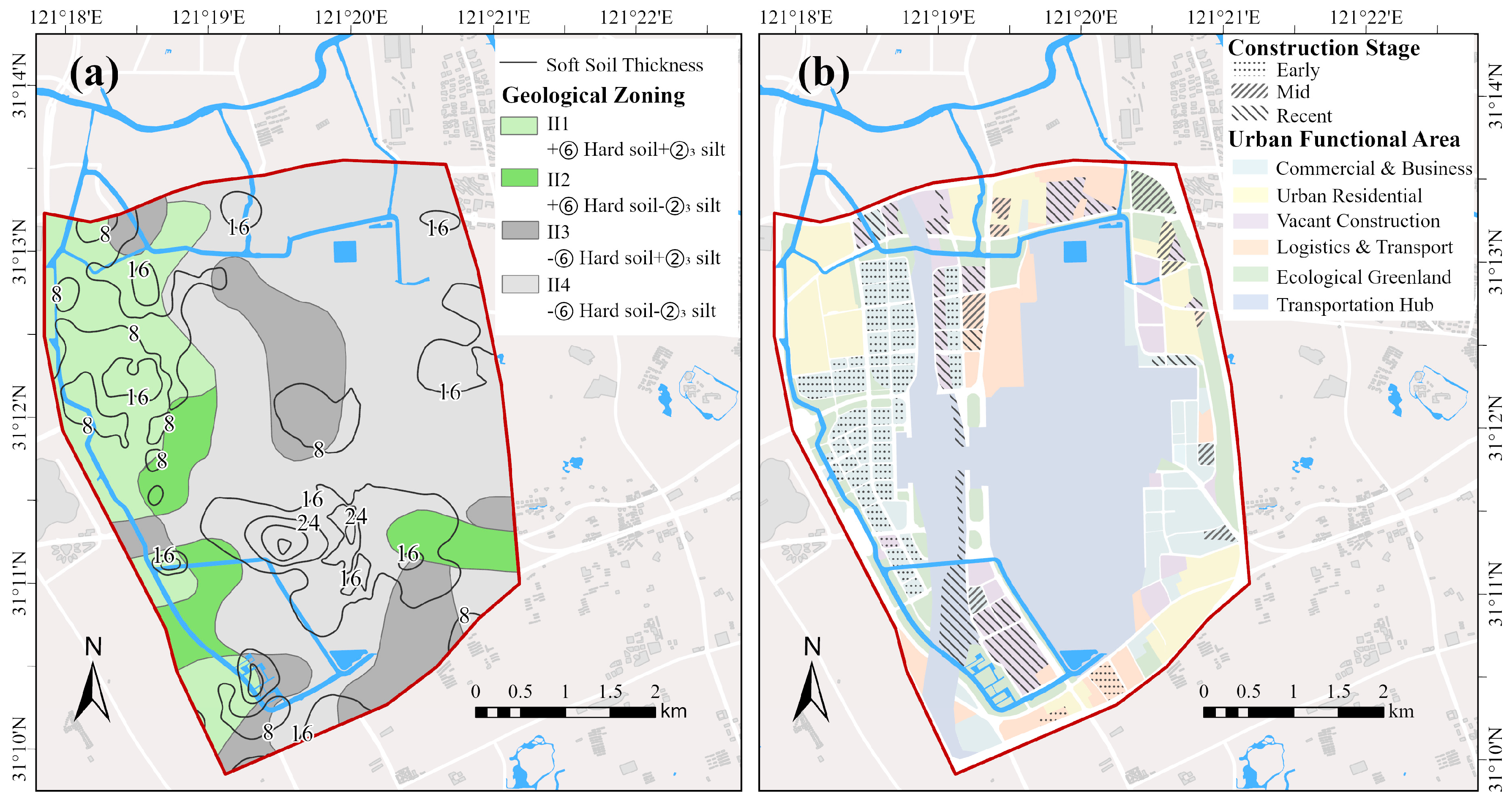
Four types of driving factors were selected to analyze the spatial differentiation of subsidence. Geological types were classified into four units based on the Geological Hazard Assessment Report of Hongqiao CBD [24]. Soft soil thickness was generated by applying Kriging interpolation [28] to 429 engineering geological boreholes obtained from the Shanghai Geological Data Information Service Platform [29]. Leave-one-out cross-validation was adopted to evaluate the accuracy of Ordinary Kriging interpolation. The results yielded an RMSE of 3.62 m and a standardized root-mean-square error of 1.02. This agreement between actual interpolation errors and modeled uncertainty validates the credibility of the soft soil thickness spatial map. Urban functional zones were extracted from the planning maps in the Hongqiao CBD Special Planning, which covers the land-use configuration for the period 2010–2019 [25]. After vectorization and spatial registration, they were classified into six categories: commercial business (CB), urban residential (UR), vacant construction (VC), logistics transport (LT), ecological greenland (EG), and transportation hub (TH). Construction stages were determined through visual interpretation of Google Earth historical imagery and divided into three stages: early (completed before 2017), mid (2017–2022), and recent (completed after 2022 or still under construction at the end of the study period) [30]. Additionally, the None stage denotes areas with no construction activity during 2015–2024, including pre-2010 structures now in post-construction consolidation, serving as the baseline for comparison. Details of each factor are summarized in Table 2. The spatial distribution of the four driving factors is illustrated in Figure 2.
Meteorological data used for seasonal deformation analysis included monthly precipitation and monthly mean temperature. Monthly precipitation was derived from the GHCN-Daily dataset provided by NOAA/NCEI [31]. Monthly mean temperature was calculated from daily maximum and minimum temperature observations at Shanghai Minhang Station (No. 58361), available from the China Meteorological Data Service Centre [32].

3. Methods

3.1. Overall Framework

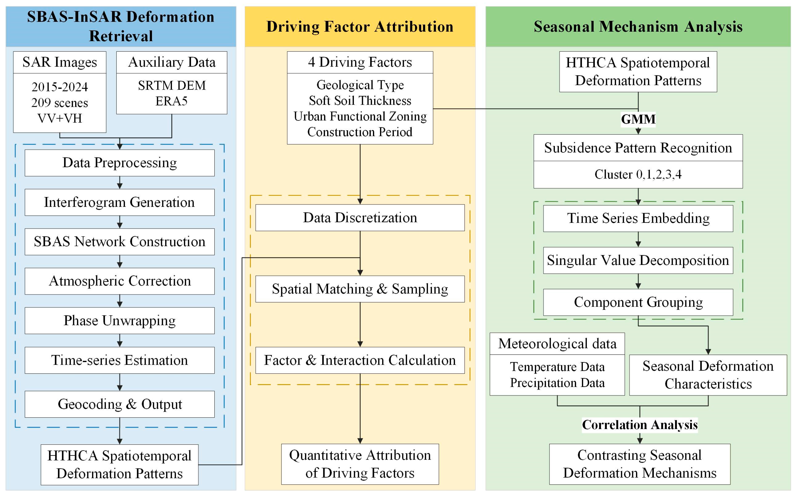
The technical framework of this study consists of three progressive modules (Figure 3), forming a complete analytical chain from deformation monitoring to mechanistic interpretation. In the first stage, SBAS-InSAR is applied to 2015–2024 Sentinel-1A images to retrieve the spatiotemporal surface deformation patterns of the HTHCA. In the second stage, GeoDetector is employed to quantify the explanatory power and pairwise interaction effects of four driving factors, based on which a five-dimensional feature vector is constructed for GMM probabilistic clustering to identify distinct deformation response patterns. In the third stage, representative time series of each cluster are decomposed via SSA to extract periodic components, followed by lag-correlation analysis with meteorological variables to decouple differential seasonal deformation mechanisms. This workflow integrates deformation retrieval, factor attribution, pattern recognition and seasonal mechanism interpretation into a unified analytical framework.

3.2. SBAS-InSAR Processing

Differential interferometry retrieves surface deformation from the phase difference between two SAR images. The relationship between the deformation phase and the line-of-sight (LOS) deformation is given by [7,8]:
Δ d = λ 4 π Δ ϕ
Following the standard InSAR sign convention, positive LOS displacement (motion toward the satellite) corresponds to a negative phase change, while negative LOS displacement (motion away from the satellite) corresponds to a positive phase change.
However, single differential interferometry is susceptible to temporal and spatial decorrelation as well as atmospheric delays, making it difficult to obtain long-time-series, high-precision deformation fields. To overcome these limitations, Berardino et al. [12] proposed the small baseline subset (SBAS) method. This method sets temporal and spatial baseline thresholds and selects only interferometric pairs with short baselines to generate M differential interferograms, thereby minimizing decorrelation. For N + 1 SAR images, the unwrapped phase at pixel x in the j-th interferogram generated from images acquired at times te and ts can be expressed as [12]:
δ ϕ j ( x ) 4 π λ d ( t E , x ) d ( t S , x ) + Δ ϕ j a t m ( x ) + Δ ϕ j t o p o ( x )
where d is the cumulative LOS deformation, and the last two terms are the atmospheric delay phase and the residual topographic phase, respectively. The unwrapped phase of each interferogram consists of the deformation increment between two consecutive acquisitions and error terms. Combining all interferograms yields a linear system of equations [12]:
A d = δ ϕ
where A is an M × (N + 1) design matrix, and d is the vector of cumulative deformations at N + 1 epochs. If all interferometric pairs are connected through short baselines, we can solve the system directly using least squares. When multiple independent subsets exist, we apply singular value decomposition to obtain the minimum-norm least-squares solution:
d = V S + U T δ ϕ
where U and V are matrices of left and right singular vectors, and S+ is the inverse of the non-zero singular values in S. This strategy links originally disconnected subsets into a complete time series covering the entire observation period.
Based on the above SBAS principle, the specific processing parameters in this study are set as follows. The temporal and spatial baseline thresholds were set to 100 days and 300 m, respectively, generating 1047 interferometric pairs in total. To suppress speckle noise, multi-looking with 4 range looks and 1 azimuth look was performed, resulting in a ground resolution of 40 m. After screening with a temporal coherence threshold of 0.6, 29,476 high-coherence pixels were preserved, occupying 95.02% of the study area. Phase unwrapping was implemented using the minimum cost flow algorithm, and unwrapping errors were corrected via phase closure and bridging methods [27,33]. All interferometric processing was performed on the Alaska Satellite Facility HyP3 cloud platform [34], and time-series inversion was carried out using the MintPy software package (version 1.6.3) [35]. The InSAR time series were referenced to a stable building located in the northwest corner of the study area, underlain by stiff soil and free from engineering disturbance.
After time-series inversion, residual phase errors need to be corrected. Jolivet et al. [27] developed a systematic tropospheric delay correction method based on global meteorological reanalysis data, using ERA5 profiles to estimate and remove the zenith wet delay. After residual DEM error correction [33,36], since only ascending Sentinel-1 data are used in this study, east–west and vertical displacements cannot be separated independently. The vertical deformation retrieval therefore relies on the assumption that horizontal displacements are relatively small. Given the flat terrain of the study area, where horizontal displacement components are generally far smaller than the vertical component for consolidation subsidence, the LOS deformation is approximated as vertical deformation [8].
d vert = d LOS cos θ
where θ is the radar incidence angle. To avoid over-interpretation, we define the result as “approximate vertical deformation” and restrict the interpretation of slight uplift and minor subsidence to within the InSAR uncertainty range.
Calculated from the averaged incidence angle across the study area, the tangent value of the incidence angle equals 0.739. On a conservative basis, horizontal movement at 2 mm per year generates a spurious vertical deformation rate of 1.48 mm per year.

3.3. GeoDetector

GeoDetector is a statistical method for quantifying the driving mechanisms of spatial heterogeneity. Its core principle is that if a factor explains the spatial distribution of a dependent variable, then stratifying by that factor yields small within-layer variance and large between-layer variance [15]. The q-statistic is defined as:
q = 1 h = 1 L N h σ h 2 N σ 2
The interaction detector identifies the interaction type (e.g., nonlinear enhancement, bi-factor enhancement, or independent effect) by comparing the q-statistic of the factor intersection q(X1X2) with the individual q-statistics of X1 and X2 [15,16]. In this study, GeoDetector is used to quantify the individual contributions and pairwise interaction effects of the four driving factors.
To satisfy the input requirements of GeoDetector, the continuous soft soil thickness is discretized into four classes: <8, 8–16, 16–24, and >24 m. Robustness validation with 3, 4, and 5 quantile-based classifications yielded identical factor rankings and interaction outcomes, proving conclusions are insensitive to discretization.
Risk detectors paired with t-tests were used to distinguish regions with significantly different subsidence rates for governance reference. To alleviate type I error inflation from InSAR spatial autocorrelation, pixels were aggregated to a 200 m × 200 m grid. Unchanged factor and interaction results after aggregation confirm no bias from spatial pseudo-replication.

3.4. Gaussian Mixture Model

The Gaussian mixture model (GMM) treats the data as a mixture of K multivariate Gaussian distributions, with the probability density function given by [37]:
p ( x ) = k = 1 K π k N x μ k , Σ k
where πk is the mixing weight, and μk and Σk are the mean vector and covariance matrix of the k-th component, respectively.
Unlike hard clustering algorithms such as K-means, GMM estimates parameters through the expectation-maximization algorithm and outputs the posterior probability of each sample belonging to each cluster. This soft assignment mechanism can effectively characterize the gradual spatial transitions of urban subsidence in the feature space, which is more consistent with the continuous nature of geological processes. The optimal number of clusters K is determined jointly by the Bayesian information criterion (BIC) [38], Akaike information criterion (AIC), silhouette coefficient [39], and Adjusted Rand Index (ARI) [40] stability across 20 random initializations. A minimum cluster size constraint (n ≥ 1200) is additionally applied to ensure geological representativeness.
For the main clustering, a diagonal covariance matrix was adopted to balance model flexibility and numerical stability, with a full covariance matrix tested as a sensitivity check. The two configurations produce consistent cluster assignments, and the diagonal model is used in the subsequent analysis. Three clustering schemes are compared: using only driving factors, using only deformation rates, and using the combination of both. The results show that deformation rates alone cannot produce a geologically meaningful cluster structure, while the five-dimensional feature vector integrating driving factors and deformation rates can capture more differentiated deformation response patterns. Accordingly, a feature vector is constructed by combining one-hot encoded categorical factors (geological type, construction stage, urban functional zone) with standardized continuous variables (soft-soil thickness and mean annual deformation rate).

3.5. Singular Spectrum Analysis

Singular spectrum analysis (SSA) is a non-parametric time-series decomposition method that extracts trend and periodic components without requiring a predefined basis function. Its core procedure is as follows. First, choose a window length M and embed the one-dimensional time series into an M × K trajectory matrix [20]:
X = X 1 , X 2 , , X K = x 1 x 2 x K x 2 x 3 x K + 1 x M x M + 1 x N
where K = NM + 1. The window length M determines the maximum resolvable period. Its selection requires balancing period separation capability and statistical reliability; typically, M should not exceed half the series length and should be greater than twice the period to be extracted.
Next, perform eigendecomposition of the covariance matrix:
S = X X T = U Λ U T
The magnitude of each eigenvalue λi reflects the energy contribution of the corresponding component to the original signal. Through grouping and reconstruction, the series can be decomposed into a sum of independent components:
x t = T t + S t + R t
where T(t) is the long-term trend component, S(t) is the periodic oscillation component, and R(t) is the noise residual component.
This study adopts a two-stage SSA workflow: cluster-averaged time series decomposition for high-SNR representative signals, followed by pixel-wise decomposition to map seasonal spatial patterns.
Pixels with annual amplitudes exceeding 3 mm, which is above the InSAR residual RMS of 2.94 mm, are identified through harmonic fitting and partitioned into summer-uplift and summer-subsidence groups according to the phase of the annual peak. Epoch-averaged sequences of each group are decomposed with a window length of 36 months, corresponding to three annual cycles. Sensitivity tests with window lengths of 24 and 48 months yield amplitude variations of less than 0.2 mm, confirming the robustness of the decomposition. Monte Carlo red-noise tests based on 1000 AR(1) surrogate series are then performed to assess the statistical significance of the seasonal signals. Irregular InSAR time series are resampled to monthly intervals, and signal power is integrated within ±2 frequency bins around the annual cycle to determine the 95% confidence threshold [41].
Pixel-wise SSA is subsequently implemented for all 481 qualified pixels. Cross-correlation between the isolated annual components and monthly meteorological variables is computed over lag ranges from −3 to +3 months. The Bartlett formula is applied to correct the significance for temporal autocorrelation [42]. Positive lags indicate that the meteorological variable precedes the deformation response.

4. Results

4.1. Deformation Field and Validation

4.1.1. Spatiotemporal Deformation Pattern

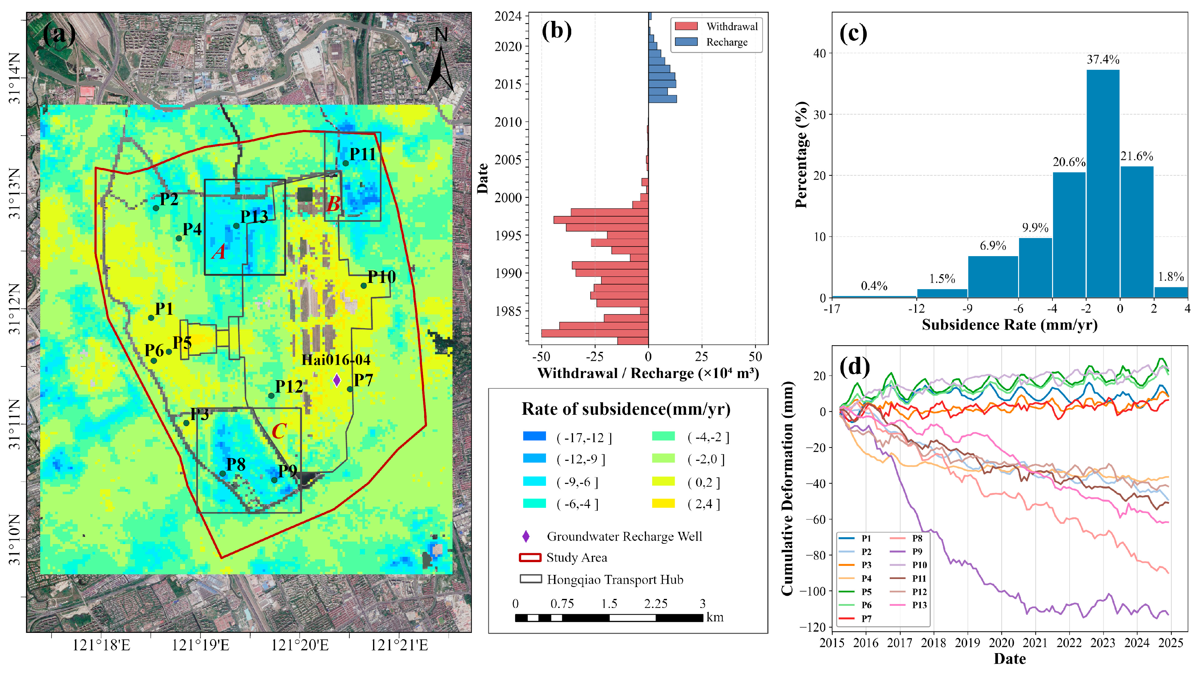
Figure 4a presents the annual average vertical deformation rate field of the HTHCA from 2015 to 2024 derived from SBAS-InSAR time-series inversion. The deformation rate histogram shows a negatively skewed distribution: over 79% of pixels fall within the slight subsidence range of −4 to 0 mm/yr, with the distribution peaking at −4 to −2 mm/yr (Figure 4c), indicating that regional subsidence has been largely controlled [14]. The mean and median subsidence rates are −1.95 mm/yr and −1.44 mm/yr, respectively; the more negative mean value indicates that a small number of rapid subsidence areas shift the overall distribution toward greater settlement magnitudes.
Three continuous subsidence funnels (A, B, C) are identified in the northern, northeastern, and southern parts of the study area, with maximum annual rates reaching −16.92 mm/yr. Funnel A corresponds to the concentrated logistics and storage zone, Funnel B overlaps with middle-stage construction sites in the east, and Funnel C is located in the southern vacant land under recent development. In contrast, the western and central parts are generally stable, with slight uplift observed around the main hub building and the western airport runway.
The H016-04 groundwater recharge well is located within this uplift zone. Its groundwater withdrawal and recharge history is plotted in Figure 4b. This well has been used for continuous artificial recharge since 2013 [6]. The spatial distribution of uplift signals is concentrated around borehole H016-04, which implies that groundwater recharge is a plausible contributor to localized land uplift via aquifer elastic recovery. The spatially restricted distribution of the subsidence funnels indicates that they are dominated by local engineering activities or soft soil consolidation, rather than regional groundwater over-exploitation [6,17].
Time-series analysis of representative points (locations marked in Figure 4a) reveals three distinct deformation patterns, with cumulative deformation curves shown in Figure 4d. The first type, represented by P8 in Funnel A, shows nearly linear continuous subsidence with approximately 80 mm cumulative settlement, reflecting persistent consolidation of thick, soft soil [43]. The second type, exemplified by P9 in Funnel C, exhibits rapid subsidence of over 100 mm from 2016 to 2021 followed by obvious deceleration, consistent with the staged attenuation of engineering disturbance [15,44]. The third type, represented by P3 and P7 in the stable western zone, fluctuates around zero deformation, indicating stable conditions with favorable geological conditions and no intense engineering disturbance. In addition, clear annual periodic fluctuations are superimposed on the long-term trend at most points, with opposite deformation directions in summer and winter [21,45], indicating a significant annual driving mechanism beyond the trend-related forces [17].

4.1.2. Validation of InSAR Results

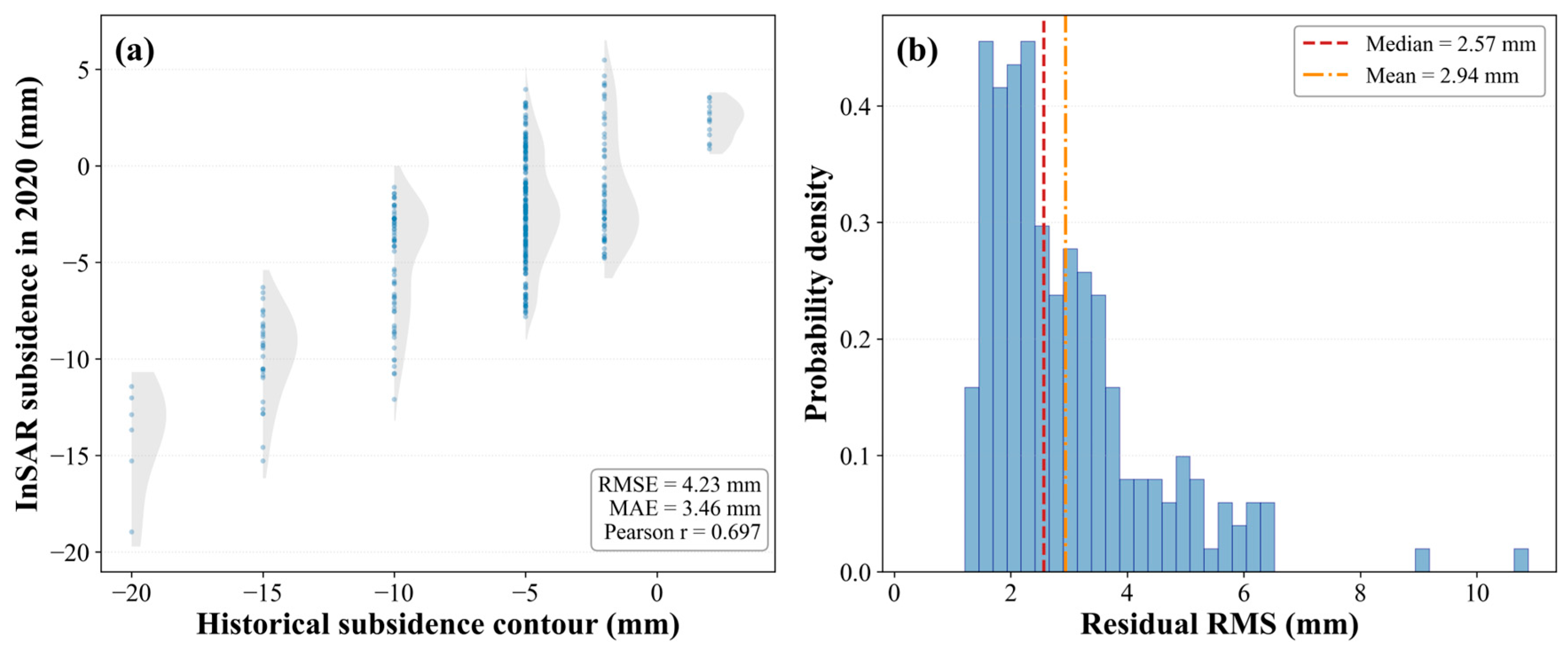
InSAR cumulative subsidence for 2020 was validated against the annual subsidence contour map documented in the Hongqiao CBD Geological Hazard Assessment Report [24]. After spatial registration, the contour values were compared with the 2020 annual deformation increment derived from InSAR (Figure 5a). The Pearson correlation coefficient r reaches 0.697 (p < 0.001, n = 555 comparison points), with an RMSE of 4.23 mm, confirming that the InSAR results capture the main subsidence features at the annual scale, though pattern agreement is stronger than absolute accuracy.
The probability density distribution of time-series residual RMS is shown in Figure 5b, with a mean value of 2.94 mm and a median of 2.57 mm. Over 80% of pixels have a residual RMS below 4 mm, reflecting satisfactory internal consistency of the SBAS-InSAR inversion [12,46]. The derived deformation rates are also consistent with published TS-InSAR results for Shanghai [13]. The reliable deformation retrieval results provide a solid data basis for subsequent driving factor attribution and pattern recognition.

4.2. Driving Factor Attribution

4.2.1. Geological Controls

The Quaternary unconsolidated deposits in the study area exceed 200 m in thickness, with widely distributed soft clay layers providing the material basis for subsidence [26]. Based on the occurrence of Layer 6 stiff clay and Layer 2–3 silty sand, the area is divided into four engineering geological subzones, transitioning from west to east with a gradual disappearance of the stiff clay layer [47]. Soft soil thickness increases from west to east and north to south, ranging from less than 8 m to over 32 m [28].
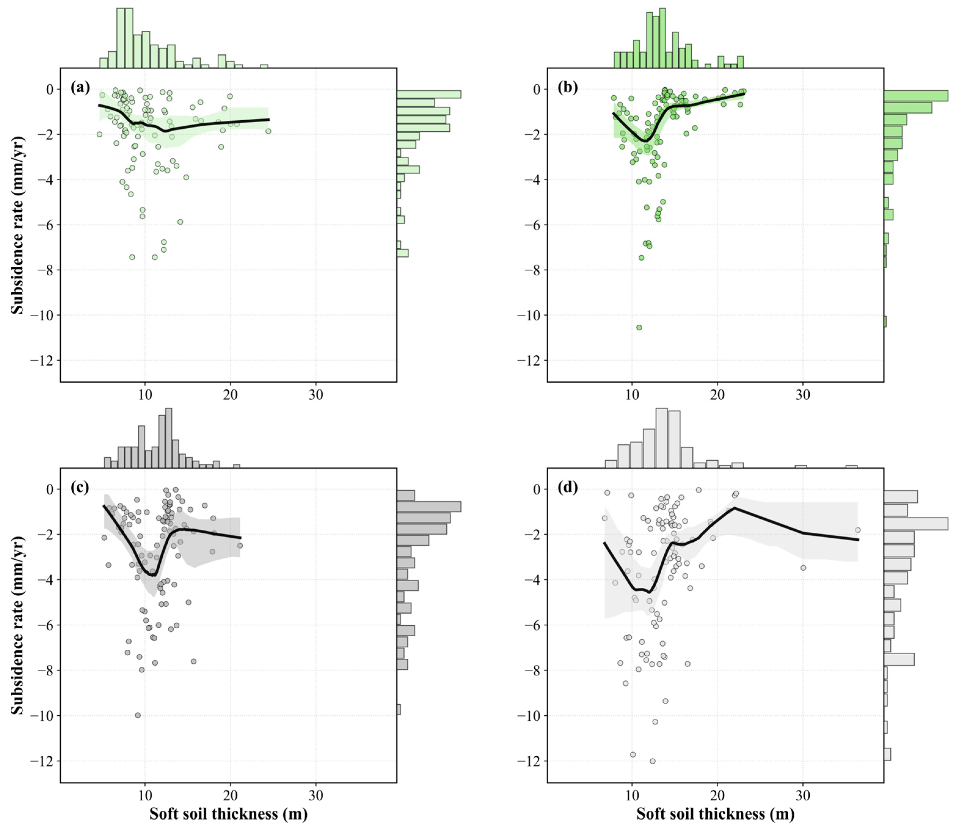
Overlay analysis (Figure 6) reveals a non-monotonic relationship between subsidence rate and soft soil thickness [48]. The highest mean subsidence rate occurs in the 8–16 m interval (−3.4 mm/yr), which also contains nearly all extreme subsidence values in the study area. When thickness exceeds 16 m, the rate decreases and stabilizes. This pattern reflects a trade-off between drainage path length and compression potential: thin layers drain quickly but have limited compressibility, while thick layers drain slowly; intermediate thicknesses exhibit the highest sensitivity under external loading [49].
A stratified analysis by construction stage confirms that this non-monotonic pattern persists within the no-construction stage (Table 3), where the 8–16 m class yields the highest mean subsidence of −1.71 mm/yr, significantly exceeding the rates of other thickness classes. This indicates that the thickness effect is not solely an artifact of co-location with active construction. Under recent construction, the 8–16 m class subsides at −5.36 mm/yr, more than twice the rate of the 16–24 m class, demonstrating that engineering disturbance substantially amplifies the thickness-dependent sensitivity.
Layer 4 soft clay in Shanghai possesses significant soil structure that is progressively lost after construction disturbance, leading to a marked increase in compressibility [50]. These characteristics indicate that the natural geological background only defines the basic susceptibility of subsidence, while the intensity of anthropogenic activities has become the key factor controlling the current spatial differentiation of subsidence.

4.2.2. Anthropogenic Controls

Urban functional zones and construction stages reflect the spatial and temporal dimensions of human disturbance on surface deformation [51]. Within the study area, TH occupies the central core, while LT are widely distributed across subsidence funnel A. VC is scattered in the northern and west-central areas, spatially overlapping with subsidence funnel C. Construction stages exhibit a west-to-east progression: early-stage projects in the west, middle-stage projects in the east and south (funnel B), and recent-stage projects in the central and southern parts (funnel C).
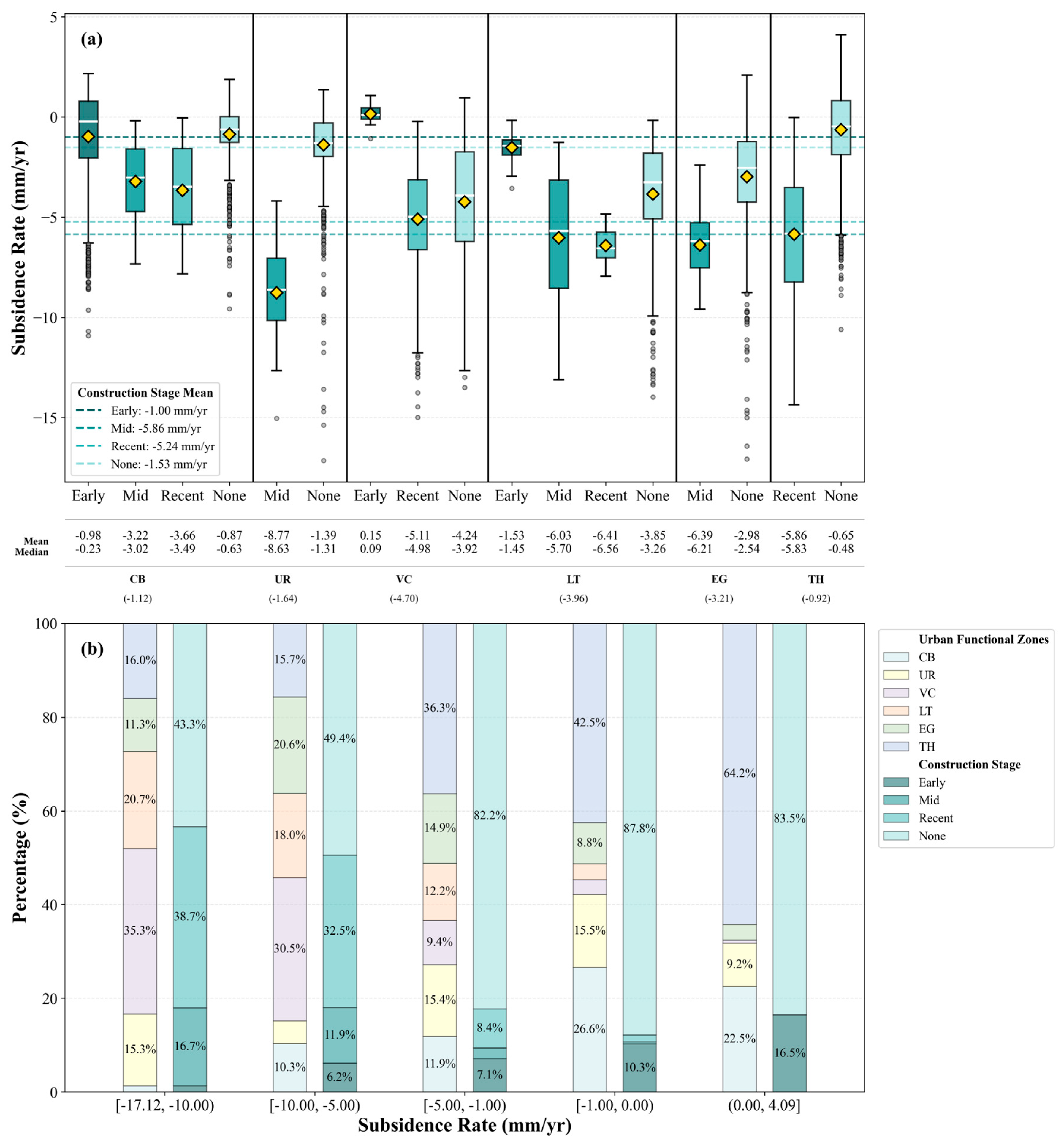
A cross-analysis of urban functional zones and construction stages (Figure 7a) disentangles the contribution of engineering activities [52]. Without engineering, subsidence rates across all functional zones remain low (−0.65 to −4.24 mm/yr), with geological background as the primary control. Engineering activities markedly intensify subsidence: the mean rate for UR in the Middle stage reaches −8.77 mm/yr (over six times the corresponding rate of UR in the None stage), while TH in the Recent stage reaches −5.86 mm/yr, far exceeding its None-stage value of −0.65 mm/yr. Different functional zones exhibit varying sensitivities: VC (−4.70 mm/yr overall mean) is affected by site grading and foundation pre-treatment, while LT (−3.96 mm/yr) are influenced by sustained dynamic loads from heavy vehicles and cargo stacking [53]. TH, in contrast, shows only −0.65 mm/yr in the None stage, indicating long-term stability after construction completion.
The stacked percentage chart (Figure 7b) reveals a progressive relationship between subsidence magnitude and engineering disturbance. In the strong subsidence interval, VC and the Recent stage account for 35.3% and 38.7%, respectively. As subsidence weakens, the proportion of the None stage increases from 82.2% (weak interval) to 87.8% (nearly stable interval). The uplift interval is dominated by TH (64.2%), all in the Early or None stage. This pattern reflects the natural decay of consolidation settlement after construction disturbance ceases [54,55], further indicating that engineering activity intensity has become the primary factor controlling deformation pattern differentiation.

4.2.3. Factor Interactions

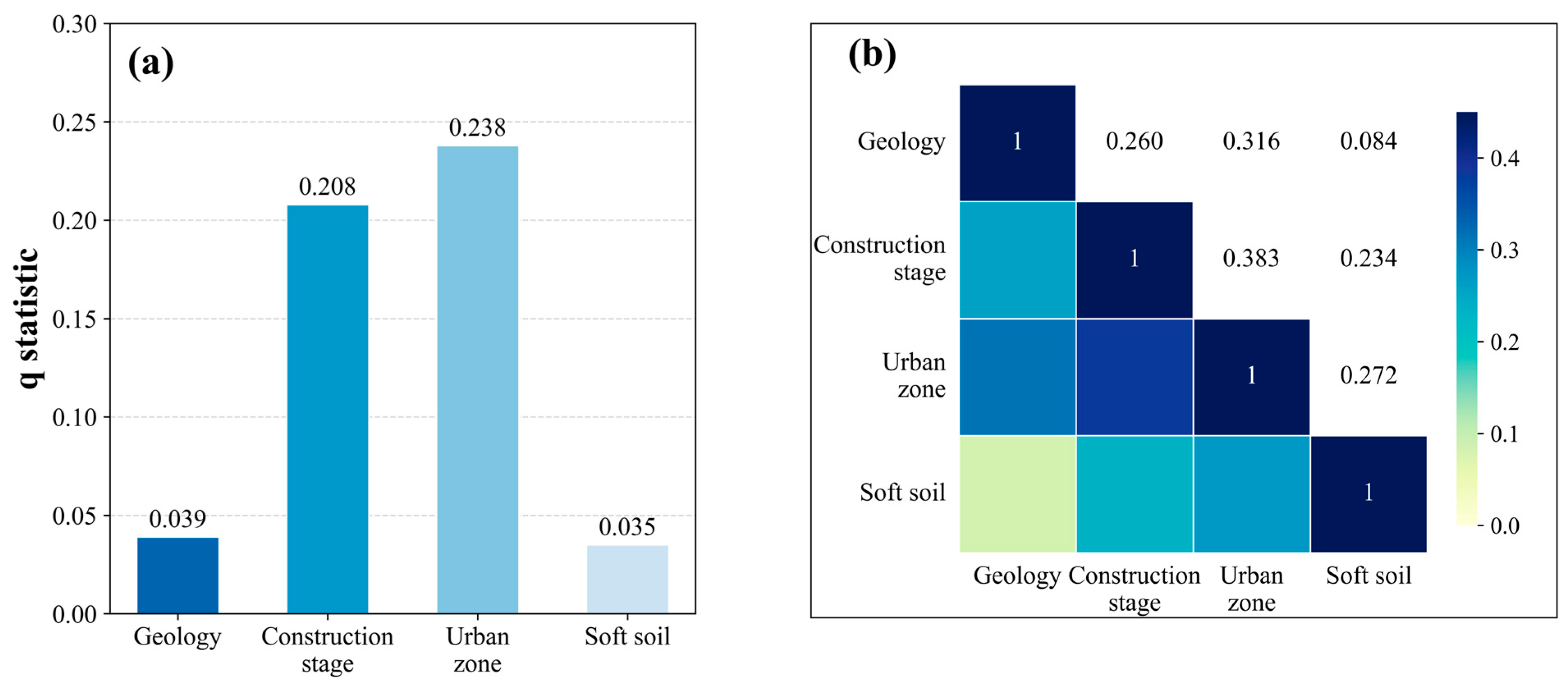
Factor detector results are shown in Figure 8a: urban functional zone (q = 0.238) and construction stage (q = 0.208) have substantially higher explanatory power than geological type (q = 0.039) and soft soil thickness (q = 0.035). The explanatory power of the dominant anthropogenic factor is approximately 5–6 times that of natural geological factors, indicating that anthropogenic factors have surpassed natural factors as the dominant influencing factors of subsidence differentiation [51,56]. This result is consistent with the findings of Minderhoud et al. [51] in the Mekong Delta and Tan et al. [56] in Shanghai. Robustness tests confirm that these attribution results are insensitive to soft-soil discretization scheme and spatial aggregation, with factor rankings and interaction types remaining unchanged.
The interaction detector further reveals widespread enhancement effects among driving factors, encompassing both nonlinear and bi-factor types (Figure 8b). The interaction q-statistic between urban functional zone and construction stage reaches 0.383, which is approximately 61% higher than the maximum single-factor q-statistic among all four drivers. When VC or LT spatially coincides with recent-stage or middle-stage construction activities, the subsidence response is substantially amplified. The interaction q-statistic between geological type and soft soil thickness is 0.084, which also exceeds the q-statistic of each factor alone. The widespread presence of interaction effects indicates that the formation of strong subsidence zones in the study area is not a simple superposition of individual factor effects.
These findings indicate that strong subsidence zones result from spatially coupled amplification between the natural foundation and anthropogenic disturbance, rather than any single factor [57,58]. The marked differences in individual factor contributions, together with the pervasive interaction effects, indicate that no single factor can independently explain the spatial differentiation of subsidence. A probabilistic classification approach integrating multi-source features is therefore required to systematically identify deformation response patterns under varying driving conditions.

4.3. GMM-Based Deformation Pattern Recognition

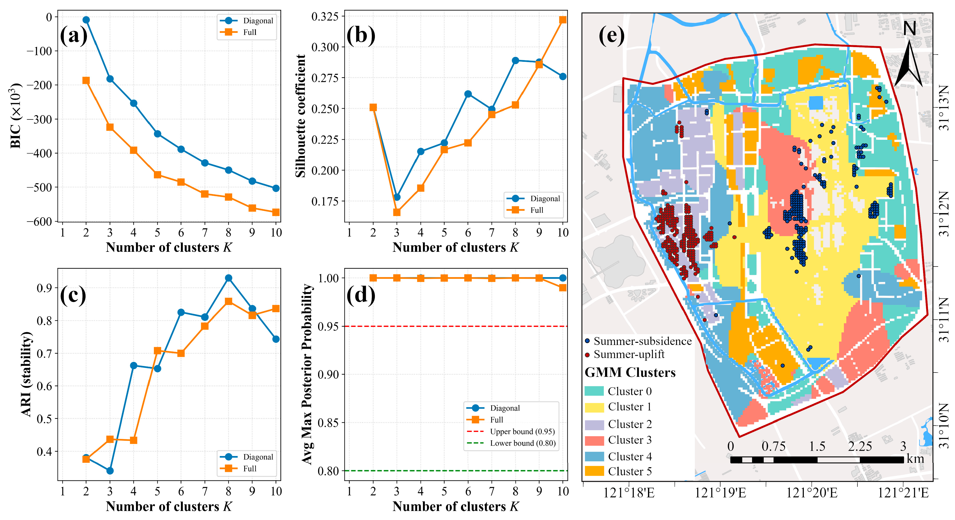
The optimal number of clusters was comprehensively determined via joint assessment of four metrics, including the BIC, AIC, silhouette coefficient, and ARI stability, with cluster numbers ranging from 2 to 10 (Figure 9a–d). The most prominent performance gain occurred when K increased from 5 to 6. The silhouette coefficient rose from 0.222 to 0.262, while the ARI stability metric climbed from 0.653 to 0.825. Despite marginal improvements in silhouette and ARI scores at K = 7 and K = 8, the solution for K = 8 suffers two critical drawbacks. First, the smallest cluster merely comprises 651 pixels with insufficient statistical representativeness. Second, the two newly generated high-subsidence clusters exhibit nearly identical driving factor compositions, with a trivial difference of only 0.36 mm/yr in their mean subsidence rates [59]. Although higher-K solutions (K = 9 and K = 10) achieve slightly higher silhouette and ARI values, they fragment the deformation field into an excessive number of small clusters with marginal physical distinction and reduced robustness of interpretation, and therefore were not adopted. Balancing statistical goodness-of-fit and physical interpretability, K = 6 was ultimately chosen as the optimal clustering number.
The six clusters obtained under the optimal K = 6 configuration show distinct differences in average subsidence magnitude and the composition of natural and anthropogenic driving factors (Table 4). Cluster 1 has the largest average subsidence rate of −5.65 mm/yr, and this cluster is dominated by areas with medium-thick soft soil covered by mid and recent construction activities, which suggests intensive engineering disturbance is a major contributor to severe settlement in this region. Cluster 0 records medium values for all input variables, reflecting transitional deformation features affected by overlapping multiple driving factors. Clusters 3 and 4 are mainly covered by transportation land use types but exhibit relatively weak subsidence signals, which implies transportation land use alone rarely triggers large-magnitude ground deformation. Cluster 2 is distributed over rigid geological layers with limited construction disturbance, accompanied by the lowest average subsidence rate of −1.00 mm/yr across the study area. Cluster 5 primarily occurs within Zone II3 soft soil units with few construction activities, where commercial land occupies the dominant functional proportion. Its average subsidence rate of −3.42 mm/yr sits between the low-deformation groups (Clusters 2, 3, 4) and high-deformation groups (Clusters 0, 1), presenting a moderate transitional deformation level.
Unlike hard clustering algorithms such as K-means that output exclusive discrete labels for each pixel, the GMM method adopts a probabilistic clustering framework and generates posterior probability values for all grid points. The mean maximum posterior probability across six clusters ranges from 0.75 to 0.83, which reflects generally reliable pixel classification results. Cluster boundaries do not display abrupt dividing lines but smooth probability gradients, consistent with the spatially continuous characteristics of urban land subsidence. The spatial distribution of six deformation clusters shown in Figure 9e matches regional geological divisions and urban functional layouts well [59,60], which lays a sound basis for the subsequent analysis of seasonal deformation mechanisms.

4.4. Seasonal Deformation Analysis

4.4.1. SSA Decomposition of Representative Time Series

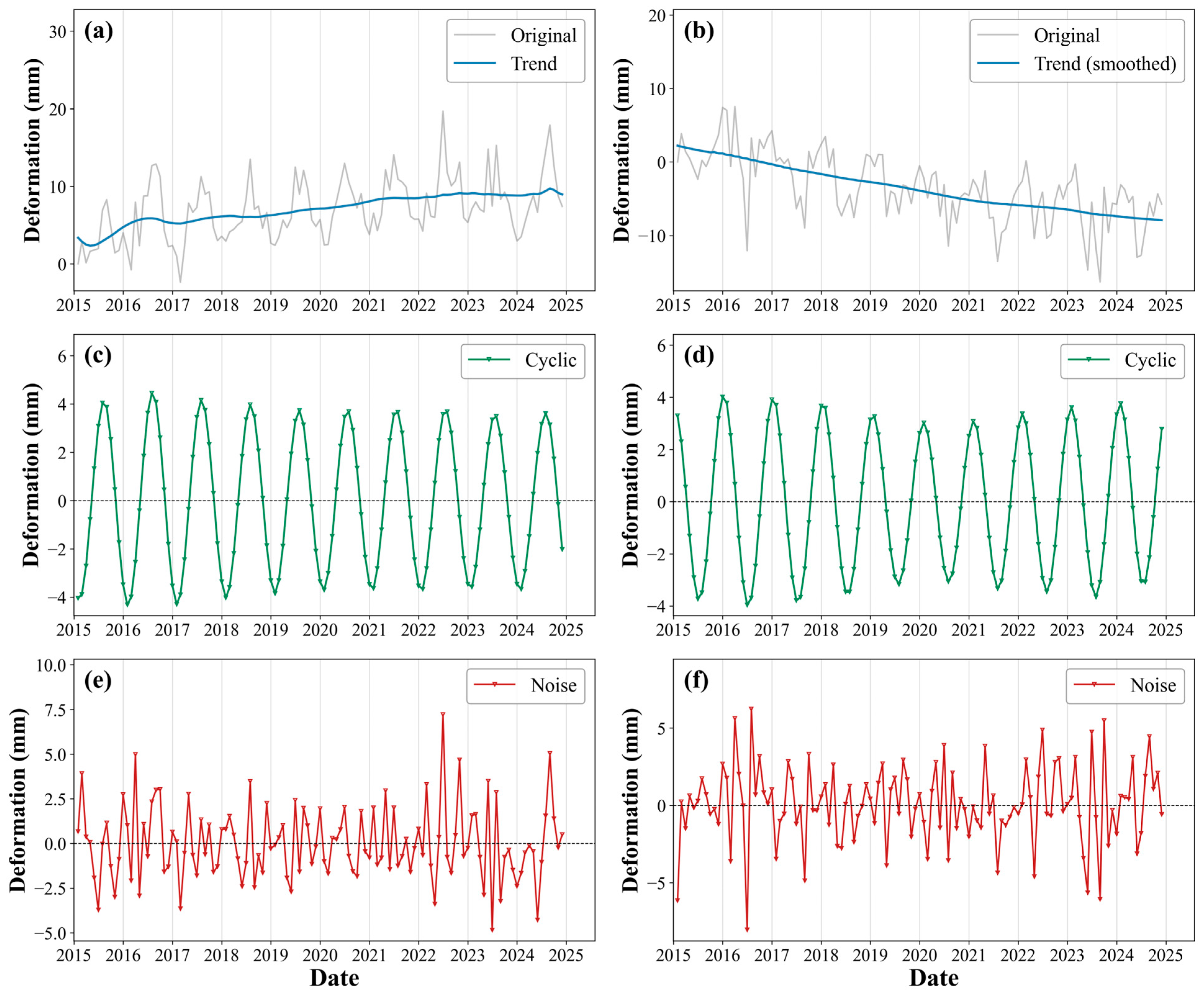
Harmonic fitting of the full InSAR time-series stack was performed pixel-wise to extract annual amplitude and phase. Pixels with annual amplitude exceeding 3 mm, the residual RMS of the SBAS-InSAR inversion, were retained, yielding 481 valid pixels. Based on the phase of the annual cycle, these pixels were partitioned into a summer-uplift group with peak-up day between days 150 and 240, and a summer-subsidence group with peak-up day between days 330 and 60. The two groups contain 233 and 223 pixels, respectively. Epoch-wise arithmetic averaging was applied within each group to suppress random noise, producing two high-signal-to-noise representative time series. SSA decomposition with a window length of 36 months was then performed on each averaged series, and the extracted trend, annual periodic, and noise components are shown in Figure 10. The annual amplitude reaches 3.90 mm for the summer-uplift group and 3.53 mm for the summer-subsidence group.
Sensitivity tests with window lengths of 24 and 48 months confirm that the extracted amplitudes are stable, with variation less than 0.2 mm. Monte Carlo red-noise testing using AR(1) surrogates confirms that both annual cycles are statistically significant at the p < 0.001 level, with amplitudes exceeding the 95% confidence thresholds [41]. Together, these results demonstrate that the two groups capture genuine, stable, and clearly distinguishable seasonal deformation signals, characterized by opposite annual phases and distinct response amplitudes, thereby providing a reliable basis for subsequent driving-force attribution [61].

4.4.2. Correlation with Climatic Drivers

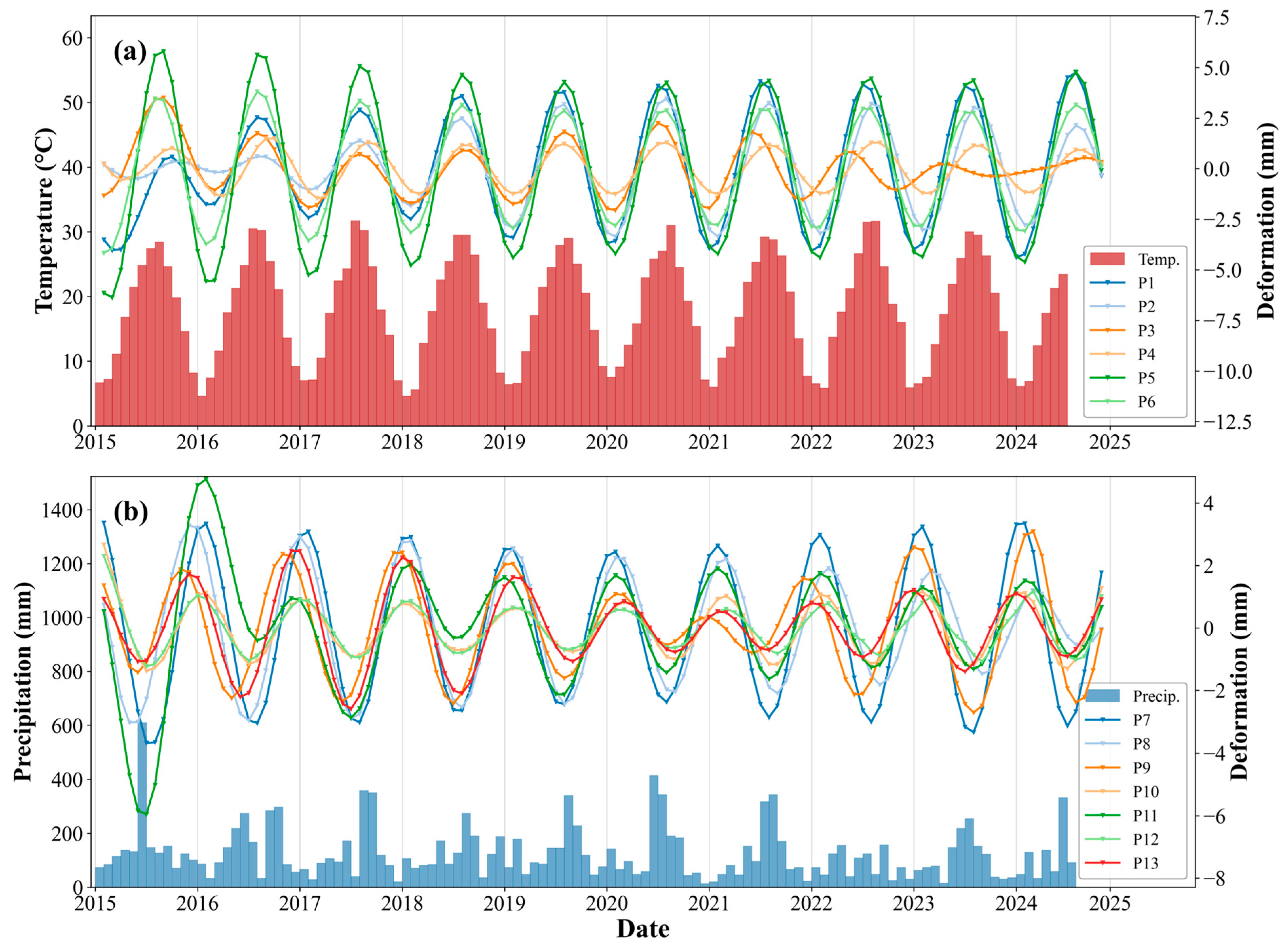
The spatial distribution of the summer-uplift and summer-subsidence pixels is presented in Figure 9e, overlaid with the spatial distribution of GMM clusters. Pixel-wise SSA was performed for all pixels to extract individual annual periodic components. For the summer-uplift group, the annual periodic component is positively correlated with temperature. The mean correlation coefficient reaches 0.57, and 54.1% of pixels are statistically significant (p < 0.05). The optimal lag concentrates at −1 month, accounting for 62.2% of pixels, with a secondary peak at 0 months accounting for 28.8%. For the summer-subsidence group, the annual periodic component is negatively correlated with precipitation. The mean correlation coefficient reaches −0.49, and 84.8% of pixels are statistically significant (p < 0.05). The optimal lag is dominated by 0 months, accounting for 69.1% of pixels. The distribution of optimal lags for both groups is summarized in Table 5.
These results reveal systematic differences between the two groups in three aspects: the meteorological variable to which they respond, the sign of the correlation, and the dominant lag. Such systematic divergence indicates that the two groups are driven by distinct seasonal forcing processes.

5. Discussion

5.1. Driving Force Transition and Multi-Factor Coupling

A coupled GeoDetector–GMM analysis reveals that urban functional zone and construction stage have surpassed geological factors as the dominant controls on subsidence differentiation [51], which is consistent with the single-factor q-statistics shown in Figure 8a. This transition, occurring under effectively controlled regional groundwater extraction, implies that engineering activity now primarily determines subsidence patterns. It also reflects a broader trajectory of urbanizing deltas: when groundwater extraction is regulated, the primary subsidence driver shifts from deep-seated aquifer compaction to shallow engineering-induced consolidation, thereby altering the depth range, spatial scale, and temporal response of land subsidence [62].
Based on their mean factor profiles (detailed parameters listed in Table 4), the six clusters are named: Transitional Zone of Special Land Use (TZSL), Strongly Human-Disturbed High Subsidence Zone (SHDZ), Hard-Soil-Protected Stable Zone (HSPS), Stable Hub Core Zone (SHCZ), Slightly Disturbed Natural Consolidation Zone (SDNZ), and Ecological–Commercial Transition Zone (ECTZ). The SHDZ combines mid- to late-stage construction with moderately thick soft soil [52]; in the HSPS, a shallow stiff clay layer (Layer 6) effectively limits load propagation and disturbance [47]; the local uplift in the SHCZ coincides spatially with recharge well H016-04, suggesting an elastic rebound from artificial recharge.
Compared with K-means-based InSAR classifications [13,14], GMM assigns each deformation pattern a clear physical label by integrating multi-source factors, and its posterior probabilities capture gradual spatial transitions that match the continuous nature of urban subsidence (Figure 9e).

5.2. Decoupling of Seasonal Deformation Mechanisms

Lag correlation analyses distinguish two distinct seasonal deformation modes extracted by pixel-wise SSA decomposition. The summer-uplift mode exhibits a positive correlation with air temperature, with the deformation peak slightly preceding or synchronous with the air temperature peak. In contrast, the summer-subsidence mode shows a negative correlation with precipitation, with the deformation response nearly synchronous with precipitation. The two seasonal deformation signals are driven by completely independent physical mechanisms and respond to different environmental forcing factors [63]. Representative intra-annual periodic deformation time series of the two deformation groups and the corresponding meteorological records are displayed in Figure 11.

5.2.1. Instantaneous Surface Surcharge Effect of Shallow Soft Strata

According to the Terzaghi one-dimensional consolidation theory and corresponding consolidation time formula, the 50% consolidation duration of local soft soil reaches approximately one year, calculated using typical geotechnical parameters, where the consolidation coefficient is on the order of 10−8 m2/s and the drainage thickness ranges from 3 to 5 m. A one-year deformation lag cannot match the near-zero seasonal lag observed for most pixels, which rules out deep consolidation as the dominant driver of annual periodic subsidence signals.
Seasonal vertical deformation is governed by instantaneous rainfall-induced overburden stress quantified via the hydrostatic load formula. Monthly summer precipitation of 150–200 mm generates an extra surface load of 1.5–2.0 kN/m2. Assuming a shallow soft-soil compression modulus (Es) of 4 MPa and a compressible layer thickness (H) of 5 m, this load produces elastic vertical compression ranging from 1.9 to 3.8 mm, consistent with the mode-averaged annual amplitude of 3.53 mm [64]. Wetting collapse of unsaturated fill further accelerates short-term deformation: infiltration reduces soil matrix suction and triggers immediate volumetric contraction without delayed drainage consolidation.

5.2.2. Thermoelastic Expansion of Built and Paved Surfaces

Pixels recording summer uplift signals are concentrated on transportation facilities and dense artificial hard surfaces. Vertical displacement is estimated with the linear thermal expansion formula for concrete and masonry materials, with a thermal expansion coefficient of 1.0–1.2 × 10⁻⁵ °C−1 [65]. For built structures and paved surfaces, the relevant thermal forcing is land surface temperature (LST) rather than ambient air temperature. According to previous MODIS LST studies over Shanghai, the mean highest summer LST is approximately 45.7 °C, while the winter value is approximately 13.9 °C, yielding a seasonal contrast of 31.8 °C [66]. With an effective structural thickness of 5–10 m, this yields a theoretical thermoelastic range of 1.6–3.8 mm, approaching the observed group-mean amplitude of 3.90 mm. The small residual difference may reflect a conservative estimate of effective structural thickness, spatial variability in LST, or minor contributions from additional local processes.
A total of 62.2% of qualified pixels exhibit an optimal lag of −1 month, consistent with surface thermal hysteresis: solar-driven LST peaks earlier than air temperature, producing a near-synchronous structural response. These results suggest that thermoelastic expansion is a plausible primary contributor to the summer-uplift signal, with residual amplitude variations across pixels likely reflecting differences in structural characteristics or local environmental conditions.

5.3. Implications for Urban Subsidence Management

The six deformation-response types may provide a preliminary macro-level framework for differentiated subsidence risk management, with the GMM map (Figure 9e) serving as a spatial zoning tool that can be aligned with Shanghai’s existing subsidence control policies [4]. Compared with empirical zoning based solely on subsidence rate thresholds, the GMM-derived zones incorporate both deformation magnitude and driving factor combinations, thus offering a potential mechanism-informed complement to conventional hazard mapping. These management implications should be regarded as preliminary, as they are derived from statistical associations and inferred mechanisms rather than from validated geotechnical models.
For the SHDZ, optimizing development timing and intensity could help avoid simultaneous large-scale construction in moderately thick soft-soil areas, thereby mitigating superimposed settlement. In the TZSL and the SDNZ, future high-density loads might need to be restricted given the thick soft-soil layers and their consolidation potential. The HSPS, with its favorable geology, appears potentially suitable for priority development, although thermal fatigue of large infrastructure could still require attention. The ECTZ, currently exhibiting moderate subsidence without active construction, warrants cautious consideration in future loading to avoid triggering accelerated settlement.
The local uplift in the SHCZ could lend support to considering expanded artificial recharge as a potential compensation measure, provided hydrogeological conditions are adequately characterized; this strategy might prove transferable to other subsidence centers. Moreover, the identified hydro-mechanical loading mechanism could point to possible synergies between urban stormwater management and subsidence control through sponge-city measures that enhance infiltration and reduce instantaneous rainfall loading on shallow soft soils [62]. It should be noted that sponge-city measures primarily regulate the surface hydrological response and are likely to have limited effect on subsidence driven by deep-seated groundwater changes; their effectiveness is thus expected to be most pronounced in the soft-ground areas where hydro-mechanical loading dominates.

5.4. Limitations and Future Perspectives

The “GeoDetector–GMM–SSA” framework has been validated in the HTHCA, yet its generalizability requires testing in other soft-soil urban settings, such as the wider Shanghai region or the Yangtze River Delta. Furthermore, all deformation results are derived from single-track ascending Sentinel-1 observations, where line-of-sight displacements are approximated as vertical deformation. Minor horizontal displacement components are neglected, which introduces a small degree of uncertainty in the estimated seasonal signal amplitudes.
A limitation of the current factor system is the absence of underground space development intensity and continuous shallow groundwater level data, which are not publicly accessible for the study area. The Construction Stage and Urban Functional Zone factors partly capture surface and shallow subsurface engineering disturbance, and the localized uplift in the SHCZ is interpreted using available recharge records from well H016-04. Methodologically, unsupervised classifiers like self-organizing maps could be introduced for cross-validation with the GMM results, thereby evaluating the robustness of different probabilistic models in identifying deformation response types [60]. In addition, integrating field-measured datasets such as long-term groundwater level records or soil moisture monitoring could further strengthen the physical validation of the identified seasonal mechanisms.
Notably, GeoDetector q-statistics only quantify the strength of statistical associations and cannot confirm causal relationships independently. Convergent evidence from GMM clustering, SSA phase divergence, and the spatial contrast between recharge-induced uplift and construction-induced subsidence collectively supports the conclusion that engineering activities dominate current subsidence patterns. Nevertheless, definitive causal attribution would require controlled intervention studies or physics-based numerical modeling.

6. Conclusions

Based on 209 Sentinel-1A images acquired from 2015 to 2024, this study analyzed the spatiotemporal differentiation patterns, driving mechanisms, and seasonal characteristics of surface deformation in the HTHCA via a progressive framework: SBAS-InSAR deformation monitoring, GeoDetector-based factor attribution, GMM-based pattern recognition, and SSA-based time-series decomposition. The main conclusions are as follows.
  • The average annual deformation rate in the study area is −1.95 mm/yr. Overall, subsidence is under control across most of HTHCA, yet three spatially continuous subsidence funnels, with maximum rates of approximately −17 mm/yr, persist and coincide spatially with recent engineering activity zones. In contrast, the main hub structure and the western area underlain by a stiff clay layer are generally stable, with local slight uplift observed. Cross-validation with official subsidence contour maps yields a Pearson correlation coefficient of 0.697 and an RMSE of 4.23 mm, confirming the spatial consistency of the InSAR results.
  • The dominant driving force of subsidence has shifted from natural geological factors to anthropogenic activities. Urban functional zone and construction stage are the two dominant influencing factors, with individual q-statistics of 0.238 and 0.208, respectively, substantially exceeding the contribution of geological background, with a bi-factor enhancement interaction between them (as evaluated among the four factors considered in this study). This indicates that the formation of strong subsidence zones is the result of spatially coupled amplification between the natural foundation and engineering disturbance.
  • GMM probabilistic clustering identified six deformation response types with marked differences in both driving-factor combinations and deformation magnitudes. Compared with conventional hard-classification methods, the posterior probabilities provided by GMM capture the gradual spatial transitions between deformation patterns, thereby providing a refined classification basis for differentiated subsidence management.
  • Two seasonal deformation signals with opposite phases and fundamentally distinct mechanisms coexist within HTHCA. The summer-subsidence signal is significantly negatively correlated with precipitation at a near-zero lag, consistent with surface-water loading on shallow soft soil; the summer-uplift signal is positively correlated with temperature, indicative of thermoelastic expansion of built structures and paved surfaces. These two mechanisms exhibit distinct spatial distributions that reflect different urban surface conditions.
The integrated analytical framework established in this study disentangles the deformation driving mechanisms in high-intensity urban development areas. The GMM clustering map can provide spatially explicit decision support for zone-based subsidence risk management, and the workflow offers a methodological reference for surface deformation research in other soft-soil cities facing similar challenges.

Author Contributions

Conceptualization, Z.Z. (Zhuoyu Zhang) and G.D.; methodology, Z.Z. (Zhuoyu Zhang) and G.D.; software, Z.Z. (Zhuoyu Zhang) and Y.F.; writing—original draft preparation, Z.Z. (Zhuoyu Zhang); writing—review and editing, Y.P. and G.D.; visualization, Z.Z. (Zhuoyu Zhang) and Z.Z. (Zixin Zhang); supervision, Y.P. All authors have read and agreed to the published version of the manuscript.

Funding

This research was funded by the National Natural Science Foundation of China (NSFC) (Grant Nos. 42574043, 42274033, 42304031 and 42474124), the National Key Research and Development Program of China (No. 2024YFB3909705), and the Open Fund of the State Key Laboratory of Spatial Datum (No. SKLSD2025-KF-17).

Data Availability Statement

The Sentinel-1A SAR data presented in this study are openly available from the Alaska Satellite Facility (ASF) at https://search.asf.alaska.edu/ (accessed on 15 March 2026). The SRTM DEM data are available from the United States Geological Survey (USGS) at https://earthexplorer.usgs.gov/ (accessed on 18 March 2026). The ERA5 reanalysis data are available from the Copernicus Climate Change Service (C3S) at https://cds.climate.copernicus.eu/ (accessed on 18 March 2026). The geological and meteorological data used in this study are available from the corresponding author upon reasonable request.

Acknowledgments

Sentinel-1A data used in this study were provided by the European Space Agency (ESA) through the Alaska Satellite Facility (ASF) data hub. The SRTM DEM and ERA5 reanalysis data were provided by the United States Geological Survey (USGS) and the Copernicus Climate Change Service, respectively. Geological and meteorological datasets were supported by the Shanghai Institute of Geological Survey, the China Meteorological Administration, and the U.S. National Oceanic and Atmospheric Administration. We are very grateful for the above support. In addition, the authors express their deep gratitude to the MintPy development team for providing the open-source InSAR time-series processing toolbox.

Conflicts of Interest

The authors declare no conflicts of interest.

References

  1. Xu, Y.-S.; Shen, S.-L.; Cai, Z.-Y.; Zhou, G.-Y. The state of land subsidence and prediction approaches due to groundwater withdrawal in China. Nat. Hazards 2007, 45, 123–135. [Google Scholar] [CrossRef] [Scilit]
  2. Xue, Y.-Q.; Zhang, Y.; Ye, S.-J.; Wu, J.-C.; Li, Q.-F. Land subsidence in China. Environ. Geol. 2005, 48, 713–720. [Google Scholar] [CrossRef] [Scilit]
  3. Xu, Y.-S.; Shen, S.-L.; Ren, D.-J.; Wu, H.-N. Analysis of factors in land subsidence in Shanghai: A view based on a strategic environmental assessment. Sustainability 2016, 8, 573. [Google Scholar] [CrossRef] [Scilit]
  4. He, X.-C.; Yang, T.-L.; Shen, S.-L.; Xu, Y.-S.; Arulrajah, A. Land subsidence control zone and policy for the environmental protection of Shanghai. Int. J. Environ. Res. Public Health 2019, 16, 2729. [Google Scholar] [CrossRef] [Scilit] [PubMed]
  5. Teatini, P.; Ferronato, M.; Gambolati, G.; Gonella, M. Groundwater pumping and land subsidence in the Emilia-Romagna coastland, Italy: Modeling the past occurrence and the future trend. Water Resour. Res. 2006, 42, W09402. [Google Scholar] [CrossRef] [Scilit]
  6. Xu, Y.-S.; Shen, S.-L.; Du, Y.-J. Geological and hydrogeological environment in Shanghai with geohazards to construction and maintenance of infrastructures. Eng. Geol. 2009, 109, 241–254. [Google Scholar] [CrossRef] [Scilit]
  7. Bürgmann, R.; Rosen, P.A.; Fielding, E.J. Synthetic aperture radar interferometry to measure Earth’s surface topography and its deformation. Annu. Rev. Earth Planet. Sci. 2000, 28, 169–209. [Google Scholar] [CrossRef] [Scilit]
  8. Ferretti, A.; Prati, C.; Rocca, F. Permanent scatterers in SAR interferometry. IEEE Trans. Geosci. Remote Sens. 2001, 39, 8–20. [Google Scholar] [CrossRef] [Scilit]
  9. Li, S.; Xu, W.; Li, Z. Review of the SBAS InSAR time-series algorithms, applications, and challenges. Geod. Geodyn. 2022, 13, 114–126. [Google Scholar] [CrossRef] [Scilit]
  10. Hooper, A.; Bekaert, D.; Spaans, K.; Arıkan, M. Recent advances in SAR interferometry time series analysis for measuring crustal deformation. Tectonophysics 2012, 514–517, 1–13. [Google Scholar] [CrossRef] [Scilit]
  11. Osmanoğlu, B.; Sunar, F.; Wdowinski, S.; Cabral-Cano, E. Time series analysis of InSAR data: Methods and trends. ISPRS J. Photogramm. Remote Sens. 2016, 115, 90–102. [Google Scholar] [CrossRef] [Scilit]
  12. Berardino, P.; Fornaro, G.; Lanari, R.; Sansosti, E. A new algorithm for surface deformation monitoring based on small baseline differential SAR interferograms. IEEE Trans. Geosci. Remote Sens. 2002, 40, 2375–2383. [Google Scholar] [CrossRef] [Scilit]
  13. Chong, Y.; Zeng, Q. Long-term ground deformation monitoring and quantitative interpretation in Shanghai using multi-platform TS-InSAR, PCA, and K-means clustering. Remote Sens. 2024, 16, 4188. [Google Scholar] [CrossRef] [Scilit]
  14. Li, W.; Wu, S.; Zhu, C.; Hou, H.; Zhang, X.; Wang, C.; Lian, M.; Wang, J. Evidence of subsidence control in Shanghai revealed by 10 years of InSAR observations. Remote Sens. 2025, 17, 3954. [Google Scholar] [CrossRef] [Scilit]
  15. Wang, J.-F.; Xu, C.-D. Geodetector: Principle and prospective. Acta Geogr. Sin. 2017, 72, 116–134. [Google Scholar] [CrossRef]
  16. Wang, J.-F.; Zhang, T.-L.; Fu, B.-J. A measure of spatial stratified heterogeneity. Ecol. Indic. 2016, 67, 250–256. [Google Scholar] [CrossRef] [Scilit]
  17. Zhu, L.; Gong, H.; Li, X.; Wang, R.; Chen, B.; Dai, Z.; Teatini, P. Land subsidence due to groundwater withdrawal in the northern Beijing Plain, China. Eng. Geol. 2015, 193, 243–255. [Google Scholar] [CrossRef] [Scilit]
  18. Wu, J.; Xie, H.; Wu, Q.; Zhang, T.; Xian, Y.; Xie, L.; Fan, W.; Shu, Y.; Liu, Z. SBAS-InSAR-based spatiotemporal characteristics, driving factors, and land use conflict detection of land subsidence: A case study of Huainan City. Remote Sens. 2026, 18, 837. [Google Scholar] [CrossRef] [Scilit]
  19. Tsai, P.-W.; Kuo, C.-Y.; Chen, Y.-C.; Chen, R.-F. Application of statistical cluster analysis and multitemporal surface displacement data for the analysis of slope subzone activity. Chin. J. Soil Water Conserv. 2023, 54, 119–129. (In Chinese) [Google Scholar]
  20. Ghil, M.; Allen, M.R.; Dettinger, M.D.; Ide, K.; Kondrashov, D.; Mann, M.E.; Robertson, A.W.; Saunders, A.; Tian, Y.; Varadi, F. Advanced spectral methods for climatic time series. Rev. Geophys. 2002, 40, 2000RG000092. [Google Scholar] [CrossRef] [Scilit]
  21. Zhang, S.; Si, J.; Niu, Y.; Zhu, W.; Fan, Q.; Hu, X.; Zhang, C.; An, P.; Ren, Z.; Li, Z. Surface deformation of expansive soil at Ankang Airport, China, revealed by InSAR observations. Remote Sens. 2022, 14, 2217. [Google Scholar] [CrossRef] [Scilit]
  22. Walwer, D.; Gonzalez-Santana, J.; Wauthier, C.; Calais, E.; Ghil, M. Multichannel singular spectrum analysis (M-SSA) of InSAR data sets: Data-adaptive interpolation and decomposition of Sentinel-1 time-series at Pacaya Volcano, Guatemala. Geophys. J. Int. 2025, 242, ggaf257. [Google Scholar] [CrossRef] [Scilit]
  23. Rana, D.; Dadkhah, H.; Ghaderpour, E.; Bozzano, F.; Mazzanti, P. Monitoring Slow-Moving Landslides through PS-InSAR and Antecedent Precipitation Index: A Case Study of Petacciato, Italy. Int. J. Remote Sens. 2026, 47, 2605–2634. [Google Scholar] [CrossRef] [Scilit]
  24. Shanghai Institute of Geological Survey. Geological Hazard Risk Assessment Report for the Main Functional Unit (HQ1) of Hongqiao Business District (2021 Annual Updated Results); Shanghai Institute of Geological Survey: Shanghai, China, 2021. [Google Scholar]
  25. Yang, L.; Wu, H.; Gan, L. A Review on the Ten-Year’s Development of Hongqiao Terminal and Hongqiao Central Business District. Urban Transp. China 2021, 19, 42–50. (In Chinese) [Google Scholar]
  26. Gong, S.-L.; Li, C.; Yang, S.-L. The microscopic characteristics of Shanghai soft clay and its effect on soil body deformation and land subsidence. Environ. Geol. 2008, 56, 1051–1056. [Google Scholar] [CrossRef] [Scilit]
  27. Jolivet, R.; Grandin, R.; Lasserre, C.; Doin, M.-P.; Peltzer, G. Systematic InSAR tropospheric phase delay corrections from global meteorological reanalysis data. Geophys. Res. Lett. 2011, 38, L12305. [Google Scholar] [CrossRef] [Scilit]
  28. Li, X.-J.; Wang, C.-H.; Zhu, H.-H. Kriging interpolation and its application to generating stratum model. Rock Soil Mech. 2009, 30, 157–162. (In Chinese) [Google Scholar]
  29. Shanghai Geological Data Information Service Platform. Available online: https://dzzl.ghzyj.sh.gov.cn/sigs-service-platform/ (accessed on 12 April 2026).
  30. Google LLC. Google Earth Pro (Version 7.3.7.1094) [Software], Google LLC: Mountain View, CA, USA, 2026. Available online: https://www.google.com/earth/ (accessed on 12 April 2026).
  31. National Centers for Environmental Information; National Oceanic and Atmospheric Administration. Global Historical Climatology Network-Daily (GHCN-Daily), Version 3; NOAA: Washington, DC, USA, 2024. Available online: https://www.ncei.noaa.gov (accessed on 15 May 2026).
  32. National Meteorological Information Center. Daily Surface Climate Data for China (V3.0); China Meteorological Data Service Centre: Beijing, China, 2012; Available online: http://data.cma.cn (accessed on 15 May 2026).
  33. Jolivet, R.; Agram, P.S.; Lin, N.-Y.; Simons, M.; Doin, M.; Peltzer, G.; Li, Z. Improving InSAR geodesy using global atmospheric models. J. Geophys. Res. Solid Earth 2014, 119, 2324–2341. [Google Scholar] [CrossRef] [Scilit]
  34. Hogenson, K.; Kristenson, H.; Kennedy, J.; Johnston, A.; Rine, J.; Logan, T.; Zhu, J.; Williams, F.; Herrmann, J.; Smale, J.; et al. Hybrid Pluggable Processing Pipeline (HyP3): A Cloud-Native Infrastructure for Generic Processing of SAR Data (Version v10.13.0) [Computer Software], Zenodo: Geneva, Switzerland, 2020. [CrossRef] [Scilit]
  35. Zhang, Y.; Fattahi, H.; Amelung, F. Small baseline InSAR time series analysis: Unwrapping error correction and noise reduction. Comput. Geosci. 2019, 133, 104331. [Google Scholar] [CrossRef] [Scilit]
  36. Fattahi, H.; Amelung, F. DEM error correction in InSAR time series. IEEE Trans. Geosci. Remote Sens. 2013, 51, 4249–4259. [Google Scholar] [CrossRef] [Scilit]
  37. McLachlan, G.J.; Peel, D. Finite Mixture Models; Wiley Series in Probability and Statistics; John Wiley & Sons: New York, NY, USA, 2000. [Google Scholar] [CrossRef] [Scilit]
  38. Schwarz, G. Estimating the dimension of a model. Ann. Stat. 1978, 6, 461–464. [Google Scholar] [CrossRef] [Scilit]
  39. Rousseeuw, P.J. Silhouettes: A graphical aid to the interpretation and validation of cluster analysis. J. Comput. Appl. Math. 1987, 20, 53–65. [Google Scholar] [CrossRef] [Scilit]
  40. Hubert, L.; Arabie, P. Comparing partitions. J. Classif. 1985, 2, 193–218. [Google Scholar] [CrossRef] [Scilit]
  41. Groth, A.; Ghil, M. Monte Carlo Singular Spectrum Analysis (SSA) Revisited: Detecting Oscillator Clusters in Multivariate Datasets. J. Clim. 2015, 28, 7873–7893. [Google Scholar] [CrossRef] [Scilit]
  42. Francq, C.; Zakoïan, J.-M. Bartlett‘s Formula for a General Class of Nonlinear Processes. J. Time Ser. Anal. 2009, 30, 449–465. [Google Scholar] [CrossRef] [Scilit]
  43. An, B.; Jiang, Y.; Wang, C.; Shen, P.; Song, T.; Hu, C.; Liu, K. Ground infrastructure monitoring in coastal areas using time-series InSAR technology: The case study of Pudong International Airport, Shanghai. Int. J. Digit. Earth 2023, 16, 355–374. [Google Scholar] [CrossRef] [Scilit]
  44. Wang, X.; Yang, Y.; Xia, Y.; Chen, S.; She, Y. Integrating SAR and geographic information data revealing land subsidence and geological risks of Shanghai City. Appl. Sci. 2023, 13, 12091. [Google Scholar] [CrossRef] [Scilit]
  45. Li, J.; Zhou, L.; Zhu, Z.; Qin, J.; Xian, L.; Zhang, D.; Huang, L. Surface deformation mechanism analysis in Shanghai areas based on TS-InSAR technology. Remote Sens. 2022, 14, 4368. [Google Scholar] [CrossRef] [Scilit]
  46. Navarro-Hernandez, M.I.; Valdes-Abellan, J.; Tomas, R.; Lopez-Sanchez, J.M.; Ezquerro, P.; Bru, G.; Boni, R.; Meisina, C.; Herrera, G. ValInSAR: A systematic approach for the validation of differential SAR interferometry in land subsidence areas. IEEE J. Sel. Top. Appl. Earth Obs. Remote Sens. 2022, 15, 3650–3671. [Google Scholar] [CrossRef] [Scilit]
  47. Sun, W.-L. Sedimentary environment and geological genesis of upper Pleistocene “dark-green stiff clay layer” in Shanghai area. Resour. Environ. Eng. 2022, 36, 225–231. (In Chinese) [Google Scholar] [CrossRef]
  48. Wu, H.; Xu, Y.-S.; Shen, S.-L.; Chai, J.-C. Long-term settlement behavior of ground around shield tunnel due to leakage of water in soft deposit of Shanghai. Front. Archit. Civ. Eng. China 2011, 5, 194–198. [Google Scholar] [CrossRef] [Scilit]
  49. Shen, S.-L.; Wu, H.-N.; Cui, Y.-J.; Yin, Z.-Y. Long-term settlement behaviour of metro tunnels in the soft deposits of Shanghai. Tunn. Undergr. Space Technol. 2014, 40, 309–323. [Google Scholar] [CrossRef] [Scilit]
  50. Yang, K.; Jia, J. Experimental and theoretical research on deformation mechanism of disturbed soil outside excavation pit in Shanghai clay. Chin. J. Undergr. Space Eng. 2013, 9, 1266–1270. (In Chinese) [Google Scholar]
  51. Minderhoud, P.S.J.; Coumou, L.; Erban, L.E.; Middelkoop, H.; Stouthamer, E.; Addink, E.A. The relation between land use and subsidence in the Vietnamese Mekong Delta. Sci. Total Environ. 2018, 634, 715–726. [Google Scholar] [CrossRef] [Scilit] [PubMed]
  52. Du, Z.; Hay-Man Ng, A.; Ge, L. Editorial: Towards a better understanding of the correlation between the subsidence pattern and land use type. Front. Earth Sci. 2024, 12, 1434425. [Google Scholar] [CrossRef] [Scilit]
  53. Monismith, C.L.; Ogawa, N.; Freeme, C.R. Permanent deformation characteristics of subgrade soils due to repeated loading. Transp. Res. Rec. 1975, 537, 1–17. [Google Scholar]
  54. Liu, G.-B.; Ng, C.W.W.; Wang, Z.-W. Observed performance of a deep multistrutted excavation in Shanghai soft clays. J. Geotech. Geoenviron. Eng. 2005, 131, 1004–1013. [Google Scholar] [CrossRef] [Scilit]
  55. Tan, Y.; Wei, B. Observed behaviors of a long and deep excavation constructed by cut-and-cover technique in Shanghai soft clay. J. Geotech. Geoenviron. Eng. 2012, 138, 69–88. [Google Scholar] [CrossRef] [Scilit]
  56. Tan, L.; Xie, Y.; Chen, C.; Bagan, H.; Yoshida, T. Urbanization and land subsidence: Multi-decadal investigation combined SBAS-InSAR and multi-factors in Shanghai, China. Geocarto Int. 2024, 39, 2391056. [Google Scholar] [CrossRef] [Scilit]
  57. Yi, X.; Wang, L.; Ci, H.; Wang, R.; Yang, H.; Yan, Z. Monitoring of land subsidence and analysis of impact factors in the Tianshan North Slope urban agglomeration. Land 2025, 14, 202. [Google Scholar] [CrossRef] [Scilit]
  58. Zhao, B.; Yang, X.; Wu, Q.; Xiao, W.; Yang, W.; Deng, M. Uncovering the structural effect mechanisms of natural and social factors on land subsidence: A case study in Beijing. Sustainability 2022, 14, 10139. [Google Scholar] [CrossRef] [Scilit]
  59. Khalili, M.A.; Voosoghi, B.; Guerriero, L.; Haji-Aghajany, S.; Calcaterra, D.; Di Martire, D. Mapping of mean deformation rates based on APS-corrected InSAR data using unsupervised clustering algorithms. Remote Sens. 2023, 15, 529. [Google Scholar] [CrossRef] [Scilit]
  60. Rygus, M.; Novellino, A.; Hussain, E.; Syafiudin, F.; Andreas, H.; Meisina, C. A clustering approach for the analysis of InSAR time series: Application to the Bandung Basin (Indonesia). Remote Sens. 2023, 15, 3776. [Google Scholar] [CrossRef] [Scilit]
  61. Tang, W.; Zhao, X.; Motagh, M.; Bi, G.; Li, J.; Chen, M.; Chen, H.; Liao, M. Land subsidence and rebound in the Taiyuan Basin, northern China, in the context of inter-basin water transfer and groundwater management. Remote Sens. Environ. 2022, 269, 112792. [Google Scholar] [CrossRef] [Scilit]
  62. Bagheri-Gavkosh, M.; Hosseini, S.M.; Ataie-Ashtiani, B.; Sohani, Y.; Ebrahimian, H.; Morovat, F.; Ashrafi, S. Land subsidence: A global challenge. Sci. Total Environ. 2021, 778, 146193. [Google Scholar] [CrossRef] [Scilit] [PubMed]
  63. Cao, Z.; Wang, T. Water-Temperature Controlled Deformation Patterns in Heifangtai Loess Terraces Revealed by Wavelet Analysis of InSAR Time Series and Hydrological Parameters. Front. Environ. Sci. 2022, 10, 957339. [Google Scholar] [CrossRef] [Scilit]
  64. Dong, S.; Samsonov, S.; Yin, H.; Ye, S.; Cao, Y. Time-Series Analysis of Subsidence Associated with Rapid Urbanization in Shanghai, China Measured with SBAS InSAR Method. Environ. Earth Sci. 2014, 72, 677–691. [Google Scholar] [CrossRef] [Scilit]
  65. Monserrat, O.; Crosetto, M.; Cuevas, M.; Crippa, B. The Thermal Expansion Component of Persistent Scatterer Interferometry Observations. IEEE Geosci. Remote Sens. Lett. 2011, 8, 864–868. [Google Scholar] [CrossRef] [Scilit]
  66. Huang, W.; Li, J.; Guo, Q.; Mansaray, L.R.; Li, X.; Huang, J. A Satellite-Derived Climatological Analysis of Urban Heat Island over Shanghai during 2000–2013. Remote Sens. 2017, 9, 641. [Google Scholar] [CrossRef] [Scilit]
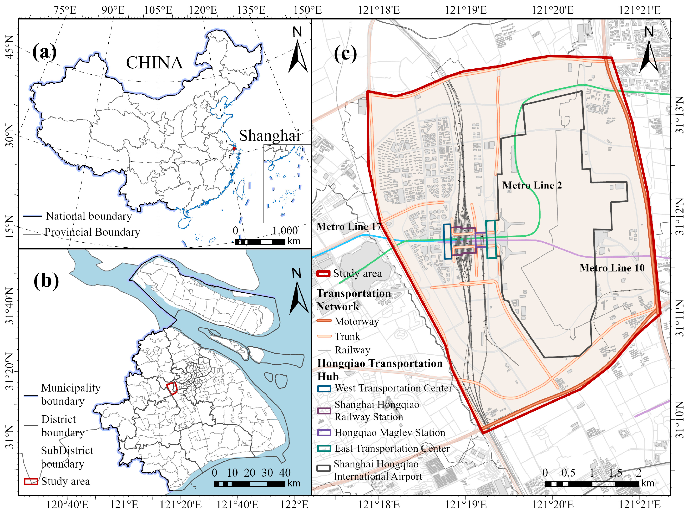
Figure 1. Location of the study area. (a) Geographical location of Shanghai in China. (b) Location of the Hongqiao Transport Hub Core Area (HTHCA) in Shanghai. (c) Scope and traffic functional layout of the study area.
Remotesensing 18 02848 g001
Figure 2. Spatial distribution of driving factors. (a) Geological type zoning and soft soil thickness contours; contour values denote soft soil thickness in meters. (b) Distribution of urban functional zones and construction stages.
Remotesensing 18 02848 g002
Figure 3. Technical flowchart of the overall research framework. The study consists of three progressive modules: SBAS-InSAR deformation inversion, quantitative attribution of driving factors, and analysis of seasonal deformation mechanisms.
Remotesensing 18 02848 g003
Figure 4. Spatiotemporal characteristics of surface deformation. (a) Annual average vertical deformation rate of the study area; A, B, and C denote the three identified main subsidence funnels. (b) Groundwater withdrawal and recharge history of Well H016-04. (c) Statistical histogram of deformation rates. (d) Cumulative deformation time series of typical monitoring points.
Remotesensing 18 02848 g004
Figure 5. Validation of SBAS-InSAR monitoring results. (a) Comparison between InSAR-derived subsidence and official contour data in 2020. (b) Probability density distribution of time-series residuals.
Remotesensing 18 02848 g005
Figure 6. Relationship between soft soil thickness and subsidence rate in different geological units. The curves are LOWESS nonlinear fitting results. (a) Zone II1. (b) Zone II2. (c) Zone II3. (d) Zone II4.
Remotesensing 18 02848 g006
Figure 7. Influence of urban functional zones and construction activities on land subsidence. (a) Box plot of deformation rates, with dashed lines indicating the mean value of each construction stage. (b) Stacked percentage bar chart for different subsidence intervals.
Remotesensing 18 02848 g007
Figure 8. GeoDetector analysis results. (a) Bar chart of single-factor q-statistic. (b) Heat map of interaction effects between driving factors.
Remotesensing 18 02848 g008
Figure 9. Determination of optimal cluster number and deformation zoning based on GMM. (a) BIC trends under diagonal and full covariance matrices against cluster number K. (b) Silhouette coefficient variations for two covariance configurations with increasing K. (c) ARI curves reflecting clustering stability under two covariance modes. (d) Mean maximum posterior probability for evaluating clustering reliability; the red dashed line represents the 0.95 upper reference bound and the green dashed line represents the 0.80 lower reference bound. (e) Spatial distribution of six deformation clusters.
Remotesensing 18 02848 g009
Figure 10. SSA decomposition results of averaged seasonal deformation time series. (a) Trend component of the summer-uplift group. (b) Trend component of the summer-subsidence group. (c) Periodic component of the summer-uplift group. (d) Periodic component of the summer-subsidence group. (e) Noise component of the summer-uplift group. (f) Noise component of the summer-subsidence group.
Remotesensing 18 02848 g010
Figure 11. Comparison between representative SSA periodic components of the two seasonal deformation groups and meteorological factors. (a) Summer-uplift group (P1–P6) and monthly mean temperature. (b) Summer-subsidence group (P7–P13) and monthly precipitation.
Remotesensing 18 02848 g011
Table 1. Parameters of InSAR and auxiliary data.
Data TypeParameterDescriptionSource
Sentinel-1ABandC-bandhttps://search.asf.alaska.edu/ (accessed on 18 March 2026)
Track DirectionAscending orbit
Number of Images209
Polarization ModeVV+VH
Imaging ModeIW
Data TypeSLC
Path171
Frame96
Timespan26 February 2015 to 23 December 2024
Average Incidence Angle36.47°
SRTM DEMResolution30 mhttps://earthexplorer.usgs.gov/ (accessed on 18 March 2026)
ERA5TimespanJanuary 2015 to December 2024https://cds.climate.copernicus.eu/ (accessed on 18 March 2026)
The incidence angle is an approximate average value. All online data were accessed between March 2026 and April 2026.
Table 2. Overview of driving factor datasets.
FactorData SourceResolution/ScaleFactor Role
Geological TypeGeological Hazard Assessment Report of Hongqiao CBD [24]1:50,000Stratigraphic constraint
Soft Soil Thickness429 boreholes, Shanghai Geological Data Platform [29]40 mCompressible layer thickness
Urban Functional ZonePlanning map, Hongqiao CBD Special Planning [25]1:50,000Surface loading pattern
Construction StageGoogle Earth historical imagery [30]1:50,000Disturbance intensity
Table 3. Stratified analysis of the relationship between soft soil thickness and subsidence rate by construction stage.
Construction StageSoft Soil Thickness ClassMean Subsidence Rate ± SD (mm/yr)Sample SizeANOVA p-Value
None<8 m−0.435 ± 0.886196<0.001
8–16 m−1.711 ± 2.4798328
16–24 m−0.670 ± 1.6181152
≥24 m−0.444 ± 1.496297
Recent8–16 m−5.364 ± 2.6591006<0.001
16–24 m−2.453 ± 1.48945
Middle8–16 m−5.853 ± 2.892341
Early8–16 m−0.999 ± 2.3201239
ANOVA p-values are reported only for stages containing at least two soft-soil thickness classes. Stages with a single thickness class are marked as ‘—’ because no between-class comparison can be performed.
Table 4. Mean values of driving factors and subsidence rates for each GMM cluster.
ClusterDominant Geological Type (%)Dominant Construction Stage (%)Dominant Urban Functional Zone (%)Soft Soil Thickness
(m)
Subsidence Rate
(mm/yr)
Max ProbDesignation
0Zone II3 (42.1%)Mid
(38.5%)
VC (35.2%)24.9 ± 6.2−2.87 ± 1.340.76Transitional Zone of Special Land Use (TZSL)
1Zone II2 (56.3%)Mid/Recent (72.8%)UR (41.6%)16.0 ± 4.8−5.65 ± 2.170.81Strongly Human-Disturbed High Subsidence Zone (SHDZ)
2Zone II1 (67.4%)None
(78.2%)
EG (52.7%)18.0 ± 5.1−1.00 ± 0.890.83Hard-Soil-Protected Stable Zone (HSPS)
3Zone II3 (59.1%)None
(81.4%)
TH (62.3%)25.8 ± 5.7−0.96 ± 0.750.79Stable Hub Core Zone (SHCZ)
4Zone II2 (51.8%)None
(65.9%)
LT (47.2%)16.0 ± 4.5−1.75 ± 1.020.77Slightly Disturbed Natural Consolidation Zone (SDNZ)
5Zone II3 (48.6%)None
(54.3%)
CB (43.5%)22.4 ± 5.9−3.42 ± 1.560.75Ecological–Commercial Transition Zone (ECTZ)
Subsidence rate and soft-soil thickness are reported as mean ± 1 standard deviation. “Dominant” refers to the category with the highest proportion within the cluster. Max prob is the mean maximum posterior probability of pixels assigned to the cluster.
Table 5. Pixel count and percentage distribution of optimal lag for two seasonal deformation groups.
Lag ValuePhysical MeaningSummer-Uplift GroupSummer-Subsidence Group
Pixel NumberRatioPixel NumberRatio
−3Deformation leads meteorology by 3 months41.7%31.3%
−2Deformation leads meteorology by 2 months166.9%00.0%
−1Deformation leads meteorology by 1 month14562.2%6328.3%
0Synchronous response6728.8%15469.1%
+1Meteorology leads deformation by 1 month10.4%20.9%
+2Meteorology leads deformation by 2 months00.0%00.0%
+3Meteorology leads deformation by 3 months41.7%31.3%
Disclaimer/Publisher’s Note: The statements, opinions and data contained in all publications are solely those of the individual author(s) and contributor(s) and not of MDPI and/or the editor(s). MDPI and/or the editor(s) disclaim responsibility for any injury to people or property resulting from any ideas, methods, instructions or products referred to in the content.