Reliability-Aware Adaptive Band Gating with Domain Expansion for Cross-Scene Hyperspectral Band Selection

Highlights

What are the main findings?

• ABG learns reliability-aware band scores from source-domain labels by coupling adaptive gating with source-domain expansion.
• Under source-domain band selection and downstream SVM evaluation, ABG is competitive on Pavia Center and strongest on HyRANK across the evaluated settings.

What are the implications of the main findings?

• Cross-scene: band selection should consider transfer utility in addition to source-domain discriminability.
• The learned gate provides original-band rankings and supports spectral-channel reduction without target-domain data during selector learning.

Abstract

Cross-scene hyperspectral band selection must reduce spectral redundancy while retaining channels that remain useful beyond the source scene. We propose Adaptive Band Gating (ABG), a source-only selector that combines frequency-domain decoupling enhancement, global and sample-specific gating, source-side spectral, spatial, morphology-inspired, and sensor-noise perturbations, and a dual-head evaluator. The selector is trained with source data and frozen before downstream evaluation. Selected bands are assessed with a radial-basis-function support vector machine on Pavia Center and HyRANK under fixed band budgets and target-label fractions from 0% to 10%. At 5% target labels, 15 selected bands achieve 96.05% overall accuracy on Pavia Center, compared with 95.41% using all 102 bands; 20 selected bands achieve 81.49% on HyRANK, compared with 79.20% using all 176 bands. Across evaluated band budgets, ABG is comparable to XGBS on Pavia Center and provides stronger results on HyRANK. Ablation experiments show that adaptive gating, frequency-domain enhancement, and source-side expansion each contribute to performance. Together, these results demonstrate that ABG learns compact and traceable original-band subsets with strong downstream transfer utility across the evaluated cross-scene settings.

1. Introduction

Hyperspectral imaging (HSI) records hundreds of narrow and contiguous spectral bands, enabling detailed discrimination of land-cover materials that are difficult to separate in broadband imagery [1]. This spectral richness benefits urban mapping, vegetation monitoring, mineral exploration, water-quality assessment, environmental surveillance, precision agriculture, and resource-constrained onboard processing, but it also introduces redundancy and computational burden. Adjacent bands can be highly correlated, some channels are degraded by noise or atmospheric effects, and high dimensionality increases overfitting risk when labels are limited. Band selection retains a subset of original wavelengths, which supports traceable channel attribution, sensor design, and efficient downstream processing without projecting the data into latent features [2].

Existing hyperspectral band-selection studies range from fixed statistical criteria to trainable selectors. Classical methods remain attractive because they are computationally efficient, easy to deploy, and directly interpretable. However, their scoring rules are usually built on shallow assumptions such as variance, correlation, separability, clustering density, or reconstruction error, and these rules often treat band importance as a fixed property of the observed scene. Such criteria are effective for reducing redundancy, but they have limited capacity to model nonlinear spectral-spatial interactions, sample-dependent band usefulness, and the coupling between discrimination and robustness under cross-scene changes. Deep learning-based selectors have therefore been introduced to learn band weights or reconstruction-oriented representations from data, providing stronger modeling capacity for complex spectral-spatial dependencies. Nevertheless, when these learned criteria are estimated from one scene or from source-domain observations, the resulting rankings can still emphasize channels whose discriminative responses are not stable after changes in scene content, acquisition date, atmospheric condition, or sensor response.

Cross-scene hyperspectral analysis requires models to handle domain shift. Inspired by the source-only domain expansion strategy of SDEnet [3], we adapt expanded source views to band selection. Cross-domain feature-selection methods such as CDIRF [4] explicitly consider transferability but often depend on shallow distance or importance measures. These observations motivate a task-level discriminability-reliability mismatch: a band may be discriminative in the source scene yet provide limited downstream utility after scene, acquisition, atmosphere, or sensor conditions change.

Three factors distinguish cross-scene from conventional single-scene band selection. First, source-discriminative channels can encode scene-specific radiometric or sensor responses. Second, one global ranking cannot fully describe sample-level spectral variation caused by mixed pixels, shadows, and local context. Third, target-free selector learning requires reliability to be evaluated through external cross-scene transfer rather than target feedback during optimization. Accordingly, we assess reliability after training through cross-scene downstream utility, multiple band budgets, component ablations, and a controlled target-label-fraction experiment.

ABG learns the band gate from source labels only. FDDEM forms a frequency-enhanced representation, the adaptive gate fuses global and sample-specific evidence, and domain expansion applies label-preserving source-side perturbations after gating. The dual-head evaluator supplies classification and contrastive signals. After source scores are averaged and the top-K bands are selected, the selector is frozen; only then are target labels used to fit the downstream SVM. Together, the source-derived views expose the selector to structured spectral-spatial variation before cross-scene evaluation.

The main contributions of this article are summarized as follows:

• We identify a mismatch between source-domain discriminability and cross-scene reliability: bands that separate source classes well may lose downstream utility under spectral-spatial shifts. Here, reliability denotes the transfer utility retained by a source-learned band ranking under unseen cross-scene conditions and is assessed through target-scene performance, band-budget behavior, component ablations, and label-fraction controls.
• We propose a reliability-aware adaptive band gating framework that learns band scores from source data by combining a global spectral prior with sample-specific responses; target samples and labels are excluded from selector learning and top-K ranking.
• We integrate source-domain expansion into band selection through spectral, spatial, morphology-inspired, and sensor-noise perturbations that broaden the source distribution while preserving source labels.
• We optimize the selector jointly with classification, contrastive, and sparsity objectives and evaluate it on the Pavia Center and HyRANK transfer tasks using band-budget, class-level, ablation, and target-label-fraction analyses.

2. Related Work

2.1. Hyperspectral Band Selection

Hyperspectral band selection has been studied as an interpretable dimensionality-reduction strategy that preserves original spectral channels while reducing redundancy and computational cost [2]. Early and classical studies commonly assign each band an importance score or search for a representative subset according to statistical separability, correlation, information content, sparse representation, or reconstruction constraints. Recent remote sensing studies have continued this line by ranking bands through extended coefficient-of-variation statistics, optimal combination strategies, multiple prioritization criteria, ensemble clustering, and cluster-wise selection [5,6,7,8,9]. These methods establish the practical value of retaining physically meaningful wavelengths, but their criteria are generally computed from fixed scene statistics and are not explicitly optimized for cross-scene robustness.

Clustering, sparse representation, and graph-based methods further address redundancy among adjacent or highly similar bands. Density-based and correlation-guided approaches identify representative centers in spectral-band space, while low-rank and spatial-spectral regularization methods model band groups through latent structures and local relationships. For example, band-density prominence clustering and related partitioning strategies improve representative-band discovery by exploiting the distribution of band similarities [6,8,10]. Despite these advances, most conventional methods estimate a single ranking from the available image and do not simulate the distribution changes encountered in source-to-target deployment.

2.2. Learning-Based and Task-Oriented Band Selection

Learning-based approaches replace hand-crafted scoring rules with trainable modules that can model nonlinear spectral interactions. EBARec-BS introduces effective band attention reconstruction for hyperspectral imagery band selection [11], BS-Nets use an end-to-end band attention and reconstruction framework [12], DARecNet-BS uses dual-attention reconstruction to learn informative channels [13], hybrid graph convolutional networks exploit graph relationships among bands [14], and BSFormer applies transformer-based reconstruction to capture long-range spectral dependencies [15]. Deep reinforcement learning has also been used to formulate band selection as a sequential decision problem for hyperspectral image classification [16]. Classification-driven feature-importance methods provide another route; for example, XGBS uses XGBoost interpretability to select task-relevant hyperspectral bands [17]. These methods strengthen adaptive representation learning, but the optimization objective is still usually formed inside a single data distribution; therefore, a band that is useful for reconstruction or classification in the source scene may remain vulnerable to target-domain spectral drift.

Task-oriented band selection has also been examined for detection, classification, and operational constraints. Such studies show that the optimal subset depends on the downstream task and that redundancy, noise, and class separability must be considered jointly. For cross-scene classification, however, task relevance alone is insufficient when the target-domain statistics are absent during training. This motivates selectors whose learned band scores are regularized not only by source labels or reconstruction quality, but also by synthetic perturbations that approximate plausible domain changes.

2.3. Cross-Scene Hyperspectral Analysis and Domain Generalization

Cross-scene hyperspectral classification is challenging because the same land-cover category can exhibit different spectral responses under changes in illumination, atmosphere, seasonal condition, sensor characteristics, or spatial context. Cross-domain feature selection addresses this issue by searching for transferable features across source and target distributions [4]. Domain-adaptation and cross-scene methods reduce distribution discrepancies through manifold alignment, deep feature alignment, two-stage domain adaptation, prototype-aligned graph learning, cooperative alignment, adversarial adaptation, joint adversarial learning, and confident learning [18,19,20,21,22,23,24,25]. These studies confirm that source-domain discrimination alone is insufficient when spectral responses shift across scenes.

2.4. Domain Expansion and Contrastive Learning

Domain expansion and contrastive learning provide mechanisms for broadening source support under limited labels. SDEnet synthesizes source-derived domains without target labels [3], while contrastive learning structures representations across semantically related views [26,27]. Generative adversarial learning has also been applied to hyperspectral classification through standard, multitask, and evolutionary formulations [28,29,30]. ABG adapts source-derived expansion and contrastive-learning principles to source-only band ranking: structured source-derived views broaden within-class variation, and contrastive objectives organize semantic relationships across those views. This combination supplies transfer-oriented supervisory signals without introducing target data into selector learning.

2.5. Positioning of ABG

The reviewed studies expose three gaps relevant to cross-scene band selection. Classical ranking, clustering, and graph methods estimate importance from fixed scene statistics; deep reconstruction or attention selectors learn nonlinear dependencies but do not directly test downstream transfer; and domain-generalization methods typically optimize classification rather than an explicit band-ranking interface.

ABG is positioned as a coupled source-only system whose contribution lies in the coordinated integration of FDDEM, global and sample-specific gating, source-derived domain expansion, and a frozen-selector downstream evaluation protocol. These components are jointly optimized to learn transferable original-band rankings from source data alone. The one-to-one correspondence between gate scores and input bands provides a traceable spectral-attribution interface, supporting wavelength-level inspection, sensor-oriented subset design, and direct comparison with other original-band selectors [2,31].

3. Materials and Methods

3.1. Overview of ABG

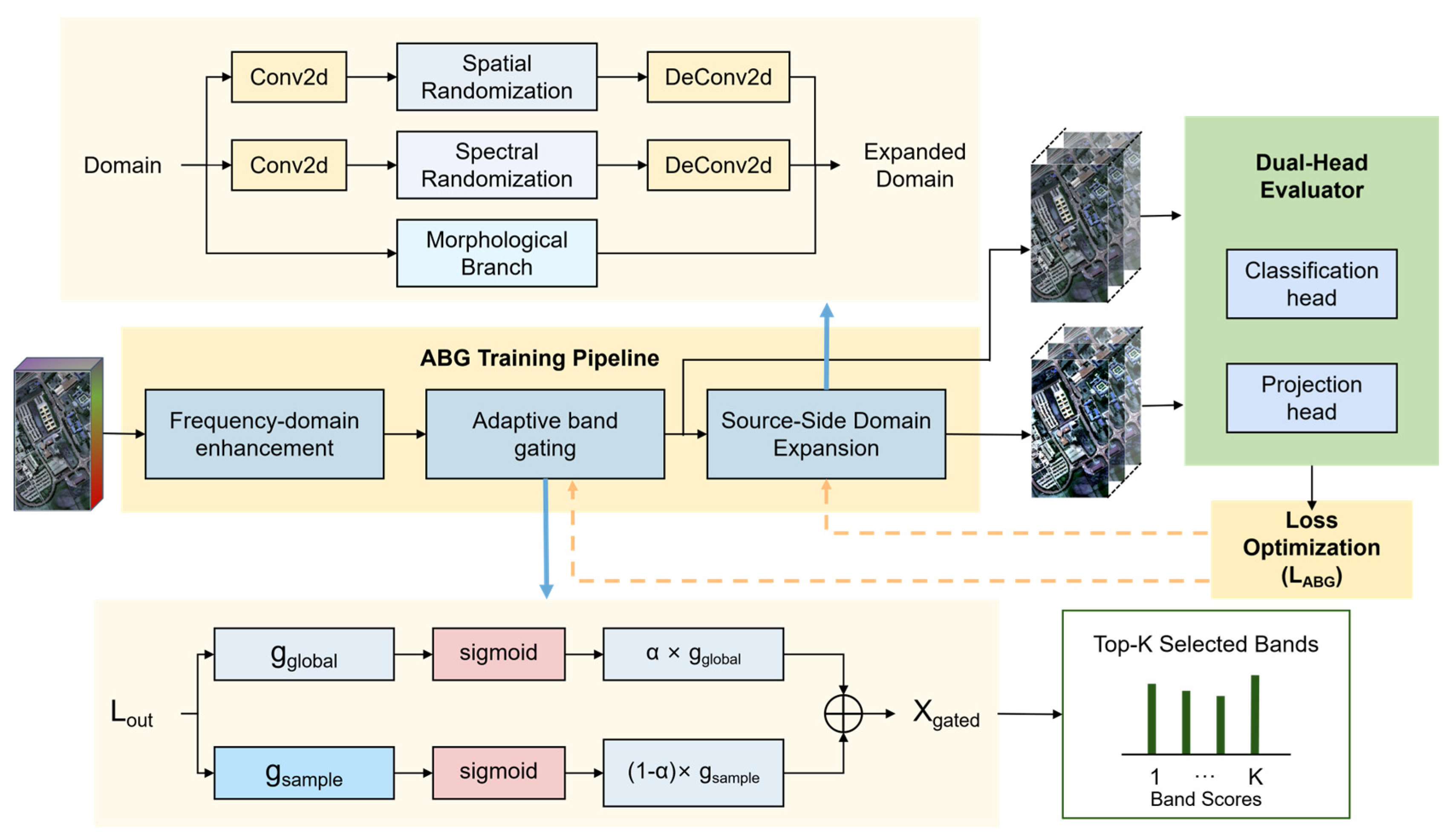
ABG is designed for source-supervised cross-scene hyperspectral band selection. Each gate output corresponds directly to an original spectral band and is applied channel-wise to the FDDEM representation. The source domain contains labeled samples; no target samples or labels are used for selector learning, hyperparameter selection, checkpoint selection, score aggregation, or top-K ranking.

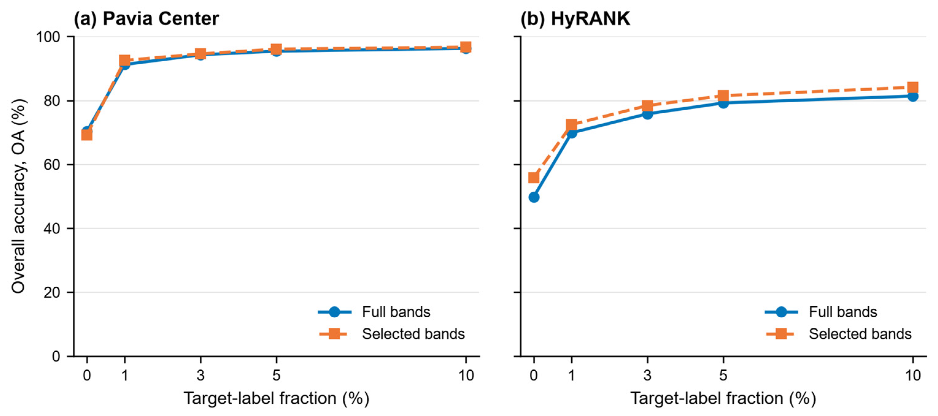
Reliability is evaluated at task level through two source-target pairs, repeated band budgets, component ablations, class-level results, and frozen-selector label-fraction controls. These complementary analyses quantify how effectively the learned ranking transfers across scenes, band budgets, model components, land-cover classes, and downstream supervision levels.

Figure 1 summarizes the source-only workflow. FDDEM produces enhanced features; the adaptive gate fuses global and sample-specific scores; source-side expansion constructs label-preserving gated views; and the dual-head evaluator provides classification and contrastive representations. The resulting source scores are averaged to obtain the final ranking. Target labels appear only after the selector is frozen, inside the downstream SVM evaluation area.

The design connects training-time representation expansion with evaluation-time transfer evidence. Frequency and spatial operations broaden the source representation, while the cross-scene results and controls reported in Section 5.1, Section 5.2, Section 5.3 and Section 5.4 provide external task-level validation of the learned ranking.

3.2. Frequency-Domain Decoupling Enhancement

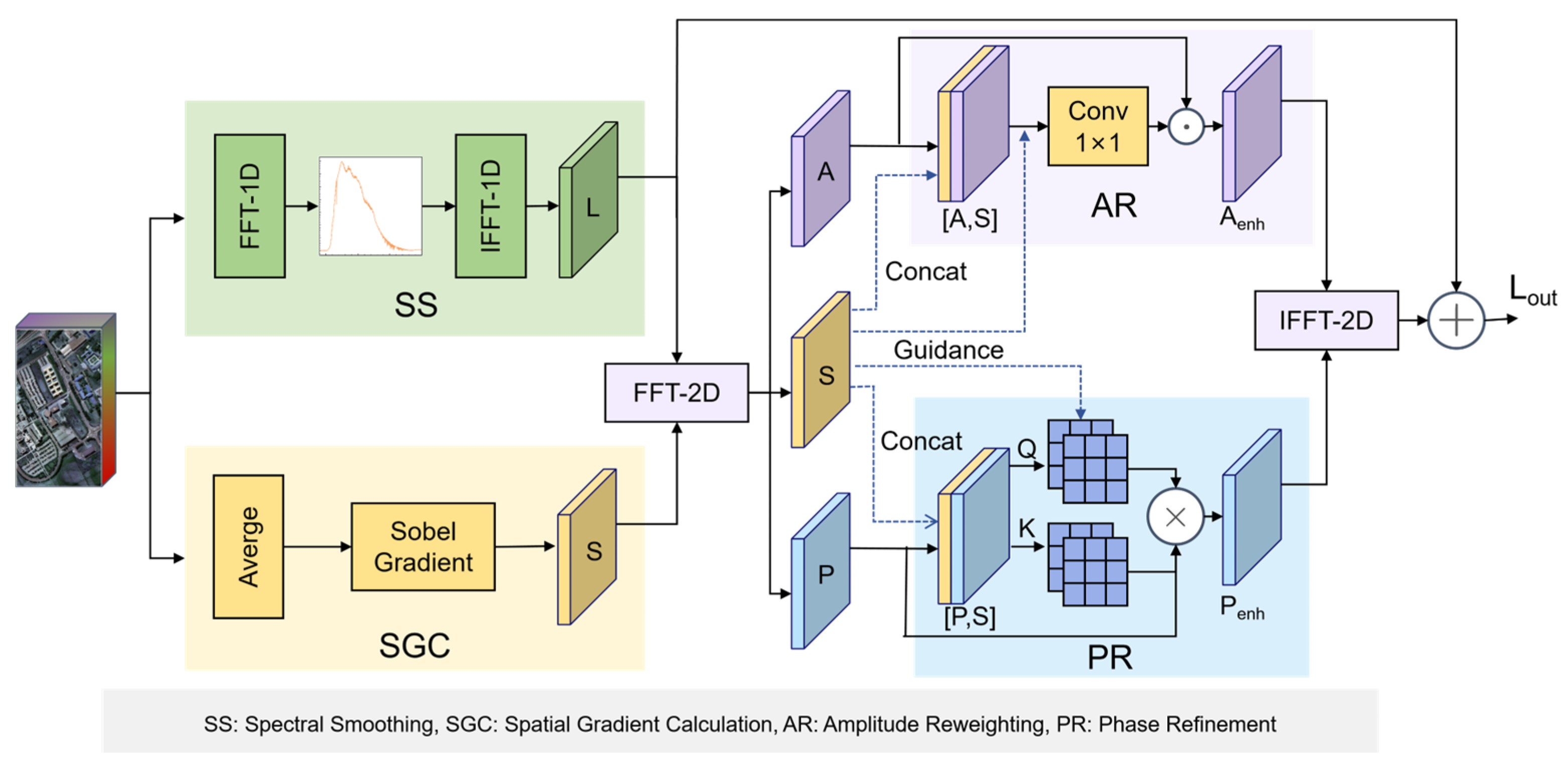
FDDEM uses complementary spectral and spatial-frequency operations to form a band-aligned representation before gating. A one-dimensional transform captures smooth inter-band trends, while two-dimensional amplitude and phase decomposition exposes frequency energy and spatial organization. Guided by a Sobel structural prior, their joint refinement yields a band-aligned representation that coordinates radiometric and structural cues before adaptive gating.

An input batch of hyperspectral cubes is denoted as $X\in {\mathbb{R}}^{N\times B\times H\times W}$, where $N$ is the batch size, $B$ is the number of spectral bands, and $H\times W$ is the spatial dimension.

For a spectral vector $x_p\in {\mathbb{R}}^B$ at spatial position $p=(h,w)$, a one-dimensional Fourier transform is first applied along the spectral dimension:

$$F_p=F_{1D}\left(x_p\right).$$

(1)

A low-pass mask $M_{K_{\mathcal{l}}}$ keeps the first $K_{\mathcal{l}}$ low-frequency coefficients and attenuates rapidly oscillating components that are often associated with noise or unstable spectral fluctuations. The smoothed spectral component is reconstructed by

$${\mathcal{l}}_p=F_{1D}^{-1}(M_{K_{\mathcal{l}}}\odot F_p)\in {\mathbb{R}}^B,L={\mathrm{S}\mathrm{t}\mathrm{a}\mathrm{c}\mathrm{k}}_p\left({\mathcal{l}}_p\right)\in {\mathbb{R}}^{N\times B\times H\times W}.$$

(2)

The cutoff $K_{\mathrm{l}}$ controls the number of retained low-frequency coefficients, and $\odot$ denotes element-wise multiplication. The low-pass component provides a smooth inter-band reference rather than assuming that every high-frequency component is noise; residual fusion with the original feature keeps localized discriminative responses available to the downstream gate and task losses.

To guide the subsequent enhancement with spatially stable structure, FDDEM computes an all-band mean image and extracts a Sobel edge prior:

$$\overline{X}={\displaystyle \frac{1}{B}}{\displaystyle \sum _{b=1}^B}{X}_b,S=\sqrt{{\left(G_x∗\overline{X}\right)}^2+{\left(G_y∗\overline{X}\right)}^2}\in {\mathbb{R}}^{N\times 1\times H\times W}.$$

(3)

where $\overline{X}$ is the all-band mean image, $G_{\mathrm{x}}$ and $G_{\mathrm{y}}$ are horizontal and vertical Sobel operators, respectively, and $\ast$ denotes convolution. The low-frequency cube $L$ is mapped by a $1\times 1$ convolution $\psi \left(·\right)$ from $B$ input bands to $D$ feature channels; $D=B$ is used so that the mapped feature channels remain one-to-one with the original spectral bands before gating. The operator $F_{2\mathrm{D}}\left(·\right)$ then applies a two-dimensional Fourier transform along the spatial dimensions.

$$C=F_{2D}\left(\psi \right(L\left)\right),A=\left|C\right|,P=\angle C.$$

(4)

The amplitude spectrum $A$ tends to be more sensitive to energy distribution, radiometric scale, and illumination-dependent variations, whereas the phase spectrum $P$ tends to preserve spatial layout and edge-related structural information. FDDEM therefore combines amplitude reweighting with structure-aware phase refinement, allowing the gate to assess each original band from a representation that jointly encodes radiometric energy and spatial organization.

After Equation (4), $A,P\in {\mathbb{R}}^{N\times D\times H\times W}$, whereas the Sobel prior is single-channel, $S\in {\mathbb{R}}^{N\times 1\times H\times W}$. The channel counts therefore differ even when the spatial supports already match. If the spatial support of $S$ differs from that of $A$ and $P$ because the Sobel and Fourier paths use different preprocessing, padding, or resampling, $I_{H,W}\left(·\right)$ first resizes $S$ to the common spatial support of $A$ and $P$; when the supports already match, the interpolation is the identity. Channel alignment is then performed as specified in Equation (5).

$$\tilde{S}=R_D\left(I_{H,W}\left(S\right)\right)\in {\mathbb{R}}^{N\times D\times H\times W}$$

(5)

In Equation (5), $I_{H,W}\left(·\right)$ denotes spatial interpolation to the size of $A$ and $P$, and $R_{\mathrm{D}}\left(·\right)$ denotes channel-wise replication. With $D=B$, the aligned prior satisfies $\tilde{S}\in {\mathbb{R}}^{N\times D\times H\times W}$; consequently, $\left[A;\tilde{S}\right]$ and $\left[P,\tilde{S}\right]$ each have shape ${\mathbb{R}}^{N\times 2\mathrm{B}\times H\times W}$. The first concatenation is mapped from $2D$ input channels to $D$ output channels by the 1 × 1 amplitude-weighting convolution in Equation (6), whereas the second supplies the structural context used to construct the query and key in Equations (7) and (8). This alignment is non-parametric and introduces no additional learnable parameters.

The amplitude path uses the structure prior to reweight frequency responses:

$$W_{amp}=\sigma \left({\mathrm{C}\mathrm{o}\mathrm{n}\mathrm{v}}_{1\times 1}^{2D\to D}\left(\left[A;\tilde{S}\right]\right)\right),A_{enh}=A\odot W_{amp}.$$

(6)

In Equation (6), $\left[A;\tilde{S}\right]$ denotes channel-wise concatenation, Conv is the learnable 1 × 1 projection from $2D$ concatenated channels to $D$ output channels, and $\sigma (\cdot )$ is the sigmoid function. The resulting map $W_{amp}$ has the same shape as $A$, and $\odot$ denotes element-wise multiplication; thus, $W_{amp}$ reweights $A$ to obtain $A_{enh}$. This operation coordinates frequency energy with the aligned spatial-boundary prior before adaptive gating.

The phase path performs structure-aware refinement with attention. The operators $W_q$, $W_k$, and $W_v$ are learnable projections. Equation (7) constructs the query $Q$ and key $K_{\mathrm{a}\mathrm{t}\mathrm{t}}$ from the concatenated phase and aligned structural prior, while the value $V$ is projected from the phase tensor:

$$Q=W_q\left(\left[P,\tilde{S}\right]\right),K_{\mathrm{a}\mathrm{t}\mathrm{t}}=W_k\left(\left[P,\tilde{S}\right]\right),V=W_v\left(P\right),$$

(7)

$$P_{enh}=\mathrm{s}\mathrm{o}\mathrm{f}\mathrm{t}\mathrm{m}\mathrm{a}\mathrm{x}\left({\displaystyle \frac{Q{K}_{\mathrm{a}\mathrm{t}\mathrm{t}}^{\top }}{\sqrt{d_k}}}\right)V.$$

(8)

In Equation (8), $d_k$ is the key dimension used to scale the dot product, and softmax normalizes the attention weights over key positions. The resulting tensor $P_{enh}$ retains the channel and spatial dimensions of $P$. Structure-aware attention therefore emphasizes phase responses supported by coherent spatial boundaries, while residual recombination keeps the enhanced representation connected to the original feature stream.

Finally, the enhanced amplitude and phase are recombined into a complex feature and transformed back to the spatial domain:

$$L_{out}=\mathfrak{R}\left(F_{2D}^{-1}\left(A_{enh}\mathrm{e}\mathrm{x}\mathrm{p}\left(i{P}_{enh}\right)\right)\right)+f_{\theta }\left(L\right).$$

(9)

In Equation (9), $\mathrm{e}\mathrm{x}\mathrm{p}\left(i{P}_{enh}\right)$ forms the complex unit-phase term, $F_{2D}^{-1}$ denotes the inverse two-dimensional Fourier transform, $\mathfrak{R}$ retains its real component, and $f_{\mathsf{\theta }}\left(L\right)$ is a learnable residual mapping of the low-frequency feature. The reconstructed branch and residual branch are added to produce the enhanced output shown in Figure 2.

3.3. Adaptive Band Gating

In cross-scene hyperspectral band selection, a subset that is discriminative in the source scene may lose utility in an unseen target scene because sensor spectral-response functions, atmospheric transmission, and illumination conditions change the observed spectra. Within a scene, local shadowing, mixed pixels, occlusion, and band-dependent noise can also change which channels are informative for an individual patch. A static global ranking cannot represent both scene-level spectral priorities and sample-level spectral-spatial variation. The adaptive band gate therefore combines a source-level global prior with patch-dependent channel reweighting, allowing less-supported bands to be softly suppressed while task-relevant channels remain active.

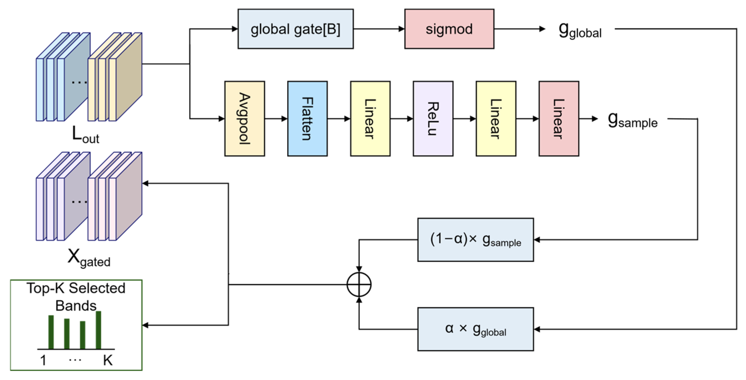
Global branch. This branch learns a scene-level spectral prior shared by all samples:

$$g_{global}=\sigma \left({\theta }_g\right),{\theta }_g\in {\mathbb{R}}^B, g_{global}\in {\left(0,1\right)}^B,$$

(10)

where ${\theta }_g$ is the global gate-logit vector defined as an internal trainable parameter of the band-gating module. It is initialized as a zero vector before training, so all bands have the same initial global activation of 0.5 after the sigmoid mapping. Since ${\theta }_g$ is shared by all input patches and updated by back-propagation with the overall objective, it represents a source-level global spectral prior rather than a feature computed from a particular sample. The sigmoid function $\sigma (\cdot )$ maps these logits into $\left(0,1\right)$, so each element of $g_{global}$ represents a soft global activation score for one spectral band.

Sample branch. This branch predicts patch-dependent band importance by applying global average pooling followed by a lightweight multilayer perceptron:

$$g_{sample}=\sigma \left(f_{\varphi }\right(\mathrm{G}\mathrm{A}\mathrm{P}\left(L_{out}\right)\left)\right), g_{sample}\in {\left(0,1\right)}^B.$$

(11)

Here, $f_{\varphi }(\cdot )$ outputs sample-specific band logits, and the sigmoid function maps them into $\left(0,1\right)$ to obtain a soft importance vector for each input patch.

The global branch encodes a shared source prior, while the sample branch responds to patch context. Their fusion combines scene-level spectral priorities with patch-specific modulation, allowing the ranking to retain a coherent global structure while adapting to local spectral-spatial variation.

The two gates are fused by a learnable scalar ${\alpha }_g=\sigma \left(a\right)$:

$$g_{fused}={\alpha }_g\cdot g_{global}+(1-{\alpha }_g)\cdot g_{sample}.$$

(12)

The fusion scalar is initialized at zero before sigmoid parameterization, producing equal initial branch weights. The fused coefficient has the same channel count as the FDDEM output and is applied element-wise.

$$X_{gated}=L_{out}\odot {\mathrm{E}\mathrm{x}\mathrm{p}\mathrm{a}\mathrm{n}\mathrm{d}}_{H,W}\left(g_{fused}\right).$$

(13)

The final band score is the source-sample average of $g_{fused}\in {\mathbb{R}}^B$. Figure 3 shows $g_{global}$, $g_{sample}$, $g_{fused}$, $X_{gated}$, and the top-K ranking interface.

3.4. Domain Expansion Module

The domain-expansion module begins from $X_{gated}$ and constructs label-preserving source-derived views. Its spectral, spatial, morphology-inspired, and sensor-noise operations expose the gated representation to complementary variations in spectral statistics, local texture and structure, and measurement noise. This structured expansion broadens source support for classification and contrastive learning and encourages transfer-oriented band rankings.

$$X_e=T\left(X_{gated}\right),T\sim \mathcal{T}.$$

(14)

The ordering is intentional: the task losses are evaluated on representations derived from the gated features, so gradients propagate through the post-gate transformations to the adaptive gate. Classification, band-level contrastive, full-to-gated consistency, and sparsity supervision therefore optimize the gate within the end-to-end computation graph, while the domain-diversity term prevents the source-derived views from collapsing to a single representation. Sensor-noise perturbation acts as an auxiliary stochastic source view with band-wise signal-to-noise variation.

$${\tilde{X}}_{b,h,w}=X_{b,h,w}+{ϵ}_{b,h,w},{ϵ}_{b,h,w}\sim \mathcal{N}\left(0,{\sigma }_b^2\right).$$

(15)

This view strengthens the retention of classification and contrastive structure under band-wise measurement-noise variation and contributes directly to the joint source objective.

Spectral randomization branch. The spectral branch models the fact that the same land-cover class may exhibit shifted spectra under different sensors or atmospheric conditions. A spectral convolution first maps the gated input to a spectral feature tensor,

$$X_{spe}=F_{spe}\left(X_{gated}\right), X_{spe}\in {\mathbb{R}}^{N\times B\times H\times W}.$$

(16)

The global mean and standard deviation of the spectral embedding are computed as

$${\mu }_{spe}={\displaystyle \frac{1}{HW}}{\displaystyle \sum _{h=1}^H}{\displaystyle \sum _{w=1}^W}{X}_{spe}^{h,w}, {\sigma }_{spe}=\sqrt{{\displaystyle \frac{1}{HW}}{\displaystyle \sum _{h=1}^H}{\displaystyle \sum _{w=1}^W}{\left(X_{spe}^{h,w}-{\mu }_{spe}\right)}^2}.$$

(17)

To generate a controllable spectral style shift, the statistics of sample $i$ are mixed with those of another sample $j$ through a learnable coefficient ${\alpha }_{\mathrm{m}\mathrm{i}\mathrm{x}}\in [0,1]$:

$${\mu }_{spe}^{mix}={\alpha }_{\mathrm{m}\mathrm{i}\mathrm{x}}\cdot {\mu }_{spe}^i+(1-{\alpha }_{\mathrm{m}\mathrm{i}\mathrm{x}})\cdot {\mu }_{spe}^j, {\sigma }_{spe}^{mix}={\alpha }_{\mathrm{m}\mathrm{i}\mathrm{x}}\cdot {\sigma }_{spe}^i+(1-{\alpha }_{\mathrm{m}\mathrm{i}\mathrm{x}})\cdot {\sigma }_{spe}^j.$$

(18)

The perturbed spectral feature is then obtained by normalization and statistic injection:

$${\tilde{X}}_{spe}=\left({\displaystyle \frac{X_{spe}-{\mu }_{spe}}{{\sigma }_{spe}+\epsilon }}\right)\cdot {\sigma }_{spe}^{mix}+{\mu }_{spe}^{mix}.$$

(19)

The statistics-exchange operation is class-conditioned to preserve source labels while varying class-consistent spectral style. It therefore enriches radiometric and sensor-response diversity at the feature-statistics level while maintaining semantic supervision.

Spatial randomization branch. The spatial branch simulates texture degradation and contrast distortion. Given the spatial feature

$$X_{spa}=F_{spa}\left(X_{gated}\right), X_{spa}\in {\mathbb{R}}^{N\times B\times H\times W},$$

(20)

the branch computes sample-wise spatial statistics ${\mu }_{spa}$ and ${\sigma }_{spa}$, mixes them with another sample to obtain ${\mu }_{spa}^{mix}$ and ${\sigma }_{spa}^{mix}$, and injects the mixed statistics into the normalized feature to obtain a perturbed spatial feature:

$${\tilde{X}}_{spa}=\left({\displaystyle \frac{X_{spa}-{\mu }_{spa}}{{\sigma }_{spa}+\epsilon }}\right)\cdot {\sigma }_{spa}^{mix}+{\mu }_{spa}^{mix}.$$

(21)

Spatial statistic exchange varies local contrast and texture strength, complementing spectral perturbation with diversity in spatial context.

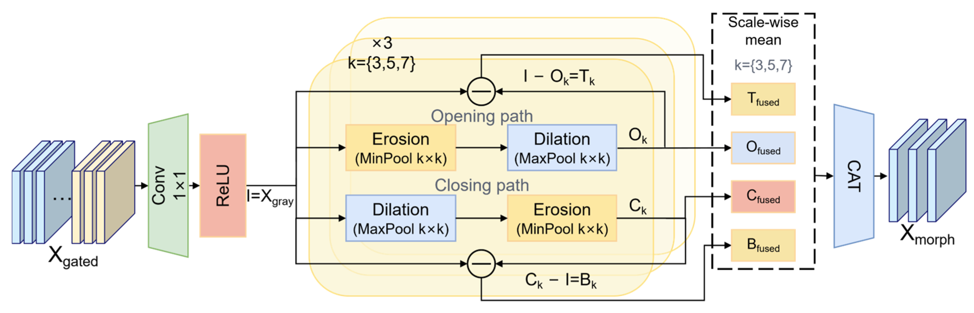
Multi-scale morphological branch. The morphology branch applies differentiable local structural transforms to $X_{gated}$. A $1\times 1$ convolution followed by a ReLU activation first compresses the $B$-channel hyperspectral feature into a single-channel structural response $X_{gray}$, providing a common intensity-like input for morphological processing. Multi-scale opening, closing, top-hat, and black-hat transformations then expose gate-derived features to systematic variations in connectivity, boundaries, and bright/dark details that characterize local land-cover structure across scenes.

$$X_{gray}=\mathrm{R}\mathrm{e}\mathrm{L}\mathrm{U}(W_{1\times 1}\ast X_{gated}+b),$$

(22)

where $\ast$ denotes convolution, $W_{1\times 1}$ and $b$ are learnable parameters, and $I=X_{gray}$. For each structuring-element size $k\in \left\{3,5,7\right\}$, opening, closing, top-hat, and black-hat responses are computed; dilation and erosion are implemented with differentiable pooling operations:

$$\begin{gathered} O_k={\mathrm{D}\mathrm{i}\mathrm{l}\mathrm{a}\mathrm{t}\mathrm{i}\mathrm{o}\mathrm{n}}_k\left({\mathrm{E}\mathrm{r}\mathrm{o}\mathrm{s}\mathrm{i}\mathrm{o}\mathrm{n}}_k\right(I\left)\right)\left(\mathrm{Opening}\right),C_k={\mathrm{E}\mathrm{r}\mathrm{o}\mathrm{s}\mathrm{i}\mathrm{o}\mathrm{n}}_k\left({\mathrm{D}\mathrm{i}\mathrm{l}\mathrm{a}\mathrm{t}\mathrm{i}\mathrm{o}\mathrm{n}}_k\right(I\left)\right)\left(\mathrm{Closing}\right), \\ {T}_k=I-O_k\left(\text{Top-Hat}\right),B_k=C_k-I\left(\text{Black-Hat}\right), \end{gathered}$$

(23)

where $O_k$, $C_k$, $T_k$, and $B_k$ denote opening, closing, top-hat, and black-hat responses at scale $k$, respectively. Opening suppresses bright details and smooths boundaries, closing fills dark gaps and strengthens connectivity, top-hat highlights bright small structures, and black-hat enhances dark details. To aggregate the multi-scale morphology, the responses are averaged across $S$ scales. In implementation, dilation and erosion are implemented by max-pooling and min-pooling operations, respectively, which are compatible with back-propagation in modern deep-learning frameworks.

$$O_{fused}={\displaystyle \frac{1}{S}}{\displaystyle \sum _{s=1}^S}{O}_{k_s},C_{fused}={\displaystyle \frac{1}{S}}{\displaystyle \sum _{s=1}^S}{C}_{k_s},T_{fused}={\displaystyle \frac{1}{S}}{\displaystyle \sum _{s=1}^S}{T}_{k_s},B_{fused}={\displaystyle \frac{1}{S}}{\displaystyle \sum _{s=1}^S}{B}_{k_s}.$$

(24)

The multi-scale morphological representation is formed by channel-wise concatenation,

$$X_{morph}=[O_{fused},C_{fused},T_{fused},B_{fused}].$$

(25)

The multi-scale responses are concatenated and diversified through adaptive normalization [32,33], enriching the source representation with scale-aware structural variations. This process is summarized in Figure 4.

Finally, the spectral, spatial, and morphological features are concatenated and decoded to produce an expanded-domain sample:

$$X_i^e=F_{dec}\left(\left[{\tilde{X}}_{spa},{\tilde{X}}_{spe},X_{morph}\right]\right).$$

(26)

An interpolated-domain sample is also constructed:

$$X_i^m=r_i{X}_i+(1-r_i)X_i^e, r_i\sim \mathcal{U}(0,1).$$

(27)

All original, gated, expanded, interpolated, and stochastic views preserve the source label and remain inside source-only selector training. Target samples and labels are absent from view construction.

3.5. Dual-Head Evaluator and Losses

The dual-head evaluator maps each source-derived view to class probabilities and a normalized contrastive embedding. For source sample i, ${\mathcal{V}}_i$ contains the original, gated, expanded, interpolated, and stochastic views. The optimization uses classification, supervised contrastive, adversarial domain-diversity contrastive, band contrastive, full-to-gated consistency, and sparse-gate terms.

$${\mathcal{V}}_i=\left\{X_i,X_i^g,X_i^e,X_i^m,X_i^{\mathrm{s}\mathrm{t}}\right\}, {\mathcal{V}}_i^{\mathrm{a}\mathrm{d}\mathrm{v}}=\left\{X_i^e,X_i^m,X_i^{\mathrm{s}\mathrm{t}}\right\}.$$

(28)

A shared spectral-spatial encoder feeds a classification head and a projection head. Classification is applied to every view $V\in {\mathcal{V}}_i$, while the normalized projection embeddings support the contrastive objectives [26,27].

The classification objective averages cross-entropy over the mini-batch and all evaluator views:

$$L_{\mathrm{c}\mathrm{l}\mathrm{s}}=-{\displaystyle \frac{1}{N}}{\displaystyle \sum _{i=1}^N}{\displaystyle \frac{1}{\left|{\mathcal{V}}_i\right|}}\sum _{V\in {\mathcal{V}}_i}{\displaystyle \sum _{c=1}^C}{y}_{i,c}\mathrm{l}\mathrm{o}\mathrm{g}{p}_{i,c}^v.$$

(29)

where $N$ is the mini-batch size, $\left|{\mathcal{V}}_i\right|$ is the number of evaluator views for sample $i$, $C$ is the number of classes, $y_{ic}$ is the one-hot label, and $p_{ic}^V$ is the predicted probability for class $c$ under view $V$.

For a minibatch collection $\mathcal{A}$ of normalized embedding–label pairs, $\mathcal{P}\left(a\right)$ contains all non-anchor indices whose supervision label matches that of anchor $a$. The following set-level supervised contrastive operator is shared by the semantic, domain-diversity, and full-to-gated consistency objectives:

$$L_{SC}(\mathcal{A})=-{\displaystyle \frac{1}{\left|\mathcal{A}\right|}}\sum _{a\in \mathcal{A}}{\displaystyle \frac{1}{\left|\mathcal{P}\left(a\right)\right|}}\sum _{p\in \mathcal{P}\left(a\right)}\mathrm{l}\mathrm{o}\mathrm{g}{\displaystyle \frac{\mathrm{e}\mathrm{x}\mathrm{p}(z_a^{\top }{z}_p∕\tau )}{\sum _{r\in \mathcal{A},r\ne a}\mathrm{e}\mathrm{x}\mathrm{p}(z_a^{\top }{z}_r∕\tau )}}.$$

(30)

In Equation (30), every embedding acts as an anchor, same-label embeddings form its positive set, and all remaining embeddings in $\mathcal{A}$ form the denominator. The label attached to each pair is the source class for semantic objectives and the class-conditioned pseudo-domain label for the domain-diversity objective. The temperature $\tau$ is fixed at 0.07 for all contrastive objectives on both benchmarks and is not tuned with target data.

$$L_{supcon}=L_{SC}\left(\left\{(z_i^V,y_i)\mid V\in {\mathcal{V}}_i,i=1,\dots ,N\right\}\right).$$

(31)

Equation (31) applies Equation (30) to the evaluator views $V\in {\mathcal{V}}_i$ using their source class labels. For the class-conditioned domain-diversity term, ${\mathcal{C}}_B$ is the set of source classes present in the mini-batch. Within each class, the gated embedding receives pseudo-domain label 0, while one virtual embedding $z_i^v$ sampled from the expanded, interpolated, or stochastic view receives label 1:

$$L_{\mathrm{c}\mathrm{o}\mathrm{n},\mathrm{a}\mathrm{d}\mathrm{v}}={\displaystyle \frac{1}{\left|{\mathcal{C}}_B\right|}}\sum _{c\in {\mathcal{C}}_B}{L}_{SC}\left(\left\{(z_i^g,0),(z_i^v,1)\mid y_i=c\right\}\right).$$

(32)

Because Equation (32) is evaluated separately within each source class, it preserves source-derived view diversity without replacing semantic supervision. Classification, supervised contrastive learning, band-level contrast, and full-to-gated consistency jointly maintain class-discriminative structure.

The band contrastive term uses the full-spectrum source representation as an anchor, the gated representation as a positive, and a random-band representation as a negative:

$$L_{\mathrm{c}\mathrm{o}\mathrm{n},\mathrm{b}\mathrm{a}\mathrm{n}\mathrm{d}}={\displaystyle \frac{1}{N}}{\displaystyle \sum _{i=1}^N}-\mathrm{l}\mathrm{o}\mathrm{g}\left[{\displaystyle \frac{\mathrm{e}\mathrm{x}\mathrm{p}\left(\mathrm{s}\mathrm{i}\mathrm{m}\left(z_{\mathrm{i}}^{\mathrm{f}\mathrm{u}\mathrm{l}\mathrm{l}},z_{\mathrm{i}}^{\mathrm{g}}\right)/\tau \right)}{\left(\mathrm{e}\mathrm{x}\mathrm{p}\left(\mathrm{s}\mathrm{i}\mathrm{m}\left(z_{\mathrm{i}}^{\mathrm{f}\mathrm{u}\mathrm{l}\mathrm{l}},z_{\mathrm{i}}^{\mathrm{g}}\right)/\tau \right)+\mathrm{e}\mathrm{x}\mathrm{p}\left(\mathrm{s}\mathrm{i}\mathrm{m}\left(z_{\mathrm{i}}^{\mathrm{f}\mathrm{u}\mathrm{l}\mathrm{l}},z_{\mathrm{i}}^{\mathrm{r}\mathrm{a}\mathrm{n}\mathrm{d}}\right)/\tau \right)\right)}}\right].$$

(33)

The full-to-gated consistency term applies the same operator to paired full-spectrum and gated embeddings carrying the same source label, thereby preserving class-relevant relationships after spectral gating:

$$L_{cons}=L_{SC}\left(\left\{(z_i^{full},y_i),(z_i^g,y_i)\mid i=1,\dots ,N\right\}\right).$$

(34)

Sparse activation is imposed on the sample-specific fused gates and on the shared global gate. Because the global gate is independent of sample index i, its contribution is written outside the mini-batch summation:

$$L_{\mathrm{s}\mathrm{p}\mathrm{a}\mathrm{r}\mathrm{s}\mathrm{e}}={\displaystyle \frac{1}{NB}}{\displaystyle \sum _{i=1}^N}{‖g_{\mathrm{i}}^{\mathrm{f}\mathrm{u}\mathrm{s}\mathrm{e}\mathrm{d}}‖}_1+{\displaystyle \frac{{‖g_{\mathrm{g}\mathrm{l}\mathrm{o}\mathrm{b}\mathrm{a}\mathrm{l}}‖}_1}{B}}.$$

(35)

The overall ABG criterion combines the classification, contrastive, consistency, and sparse-gate terms as

$$L_{\mathrm{A}\mathrm{B}\mathrm{G}}=L_{\mathrm{c}\mathrm{l}\mathrm{s}}+{\lambda }_1{L}_{\mathrm{s}\mathrm{u}\mathrm{p}\mathrm{c}\mathrm{o}\mathrm{n}}+{\lambda }_2{L}_{\mathrm{c}\mathrm{o}\mathrm{n},\mathrm{a}\mathrm{d}\mathrm{v}}+L_{\mathrm{c}\mathrm{o}\mathrm{n},\mathrm{b}\mathrm{a}\mathrm{n}\mathrm{d}}+{\lambda }_s{L}_{\mathrm{s}\mathrm{p}\mathrm{a}\mathrm{r}\mathrm{s}\mathrm{e}}+{\lambda }_c{L}_{cons}.$$

(36)

During training, the evaluator and the FDDEM–gate–expansion pathway are updated with the terms relevant to their respective optimization steps. The adaptive gate remains inside the differentiable post-gate computation graph, and the sparse term acts directly on the fused and global gate activations.

The complete source-only training and band-selection procedure is summarized in Algorithm 1.

Algorithm 1. Source-Only ABG Training and Band Selection
Line	Operation
1	Input source patches Xs, source labels ys, band count B, band budget K, τ = 0.07, and fixed loss coefficients.
2	Set the FDDEM feature width to the original spectral-band count.
3	For each source mini-batch, compute $L_{\mathrm{o}\mathrm{u}\mathrm{t}}=\mathrm{F}\mathrm{D}\mathrm{D}\mathrm{E}\mathrm{M}\left(X_{\mathrm{s}}\right)\in {\mathbb{R}}^{N\times B\times H\times W}.$
4	Compute $g_{\mathrm{g}\mathrm{l}\mathrm{o}\mathrm{b}\mathrm{a}\mathrm{l}}$ and $g_{\mathrm{s}\mathrm{a}\mathrm{m}\mathrm{p}\mathrm{l}\mathrm{e}}$ in ${\mathbb{R}}^B$ and fuse them as $g_{\mathrm{f}\mathrm{u}\mathrm{s}\mathrm{e}\mathrm{d}}$
5	Form $X_{\mathrm{g}\mathrm{a}\mathrm{t}\mathrm{e}\mathrm{d}}=L_{\mathrm{o}\mathrm{u}\mathrm{t}}$ multiplied channel-wise by $g_{\mathrm{f}\mathrm{u}\mathrm{s}\mathrm{e}\mathrm{d}}$
6	Construct spectral, spatial, morphology-inspired, and sensor-noise source views from $X_{\mathrm{g}\mathrm{a}\mathrm{t}\mathrm{e}\mathrm{d}}$
7	Evaluate original, gated, expanded, interpolated, and stochastic views with both heads.
8	Compute Lcls and Lsupcon over the evaluator views.
9	Compute Lcon,adv, Lcon,band, and Lcons using τ.
10	Compute the sparse-gate term Lsparse.
11	Update the evaluator and the FDDEM–gate–expansion pathway with the corresponding terms of LABG; post-gate task gradients propagate to the gate parameters.
12	Repeat for 400 epochs using source data only.
13	Aggregate the fused gate over source samples to obtain one score per original band.
14	Rank the B scores and retain the top-K original bands.
15	Freeze the selector before any target sample or label is used.
16	Restrict the downstream data to the selected channels and fit/evaluate the specified SVM protocol.

4. Experimental Setup

4.1. Datasets

Two cross-scene benchmarks are used. The Pavia setting transfers from Pavia University to Pavia Center, and the HyRANK setting transfers from Dioni to Loukia.

The Pavia benchmark was acquired by the Reflective Optics System Imaging Spectrometer (ROSIS) over Pavia, Italy. The Pavia University source image has a spatial size of $610\times 340$ pixels, while the Pavia Center target image has a spatial size of $1096\times 715$ pixels. Both scenes have a spatial resolution of 1.3 m per pixel. The spectral responses cover approximately 0.43–0.86 μm. Both scenes contain 102 spectral bands and seven shared urban land-cover classes for cross-scene evaluation.

The HyRANK benchmark was acquired by the Hyperion sensor onboard the EO-1 satellite under the ISPRS scientific initiative. Dioni is used as the source scene and Loukia as the target scene. Their spatial sizes are $250\times 1376$ and $249\times 945$ pixels, respectively. The imagery has a spatial resolution of 30 m per pixel. Hyperion covers the visible to shortwave-infrared range, approximately 0.4–2.5 μm. Each scene contains 176 spectral bands, and the benchmark defines 12 land-cover classes including urban, agricultural, vegetation, rock/sand, and water categories. The sample distributions are listed in

Table 1. Class sample counts for the Pavia University to Pavia Center transfer task.

No.	Class	Pavia University	Pavia Center
1	Trees	7598	3064
2	Asphalt	9248	6631
3	Brick	2685	3682
4	Bitumen	7287	1330
5	Shadow	2863	947
6	Meadow	3090	18,649
7	Bare soil	6584	5029
Total		39,355	39,332

and

Table 2. Class sample counts for the Dioni to Loukia transfer task in HyRANK.

No.	Class	Dioni	Loukia
1	Dense urban fabric	1262	206
2	Mineral extraction sites	204	54
3	Non-irrigated arable land	614	426
4	Fruit trees	150	79
5	Olive groves	1768	1107
6	Coniferous forest	361	422
7	Dense sclerophyllous vegetation	5035	2996
8	Sparse sclerophyllous vegetation	6374	2361
9	Sparse vegetated areas	1754	399
10	Rocks and sand	492	453
11	Water	1612	1393
12	Coastal water	398	421
Total		20,024	10,317

, and the visual overviews are shown in Figure 5 and Figure 6.

4.2. Baselines and Protocol

The comparison includes classical and learning-based band-selection methods: SPA-BS [34], EFDPC [35], ISSC [36], BS-Conv [12], DARecNet [13], COWOASA [37], CDIRF [4], and XGBS [17]. SPA-BS, EFDPC, and ISSC represent sparse ranking, clustering, and subspace methods, respectively. BS-Conv and DARecNet are deep reconstruction-oriented methods. COWOASA and CDIRF are cross-domain feature-selection baselines related to transferability and Relief-style feature weighting [38]. XGBS is a classification-driven baseline that uses XGBoost interpretability to rank bands from supervised source-domain information. All methods are evaluated under the same selected-band range and classifier protocol to ensure a consistent comparison.

For every band-selection method, top-K scores are learned from source data and frozen before target-label use. The primary tables use the predefined 5% target split. A complementary control evaluates 0%, 1%, 3%, 5%, and 10% target-label fractions with identical selected/full-band splits and RBF-SVM settings. At 0%, the scaler and SVM are fitted on an 80% subset of the source-domain data; at nonzero fractions they are fitted with the corresponding target training subset. Pavia uses $K=15$ of 102 bands and HyRANK uses $K=20$ of 176 bands. No target labels enter selector training, score aggregation, or ranking.

Evaluation metrics. The quantitative evaluation is derived from the confusion matrix on the held-out target-domain test subset. Overall accuracy (OA) is computed as the ratio of correctly classified pixels to all evaluated target pixels and measures global classification performance. Class-level accuracy is the recognition rate of each land-cover class, while average accuracy (AA) is obtained by averaging the class-level accuracies to assess class-balanced performance [39,40]. The Kappa coefficient measures the agreement between the predicted labels and the ground truth after excluding chance agreement, providing a complementary indicator under class-imbalanced conditions [41,42]. OA curves under different selected-band numbers are used to evaluate the sensitivity of each method to the band budget [2].

Implementation details. Patches are $13\times 13$ and the batch size is 256. ABG is trained for 400 epochs using Adam with an initial learning rate of $1\times$. The projection dimension is 128. The FDDEM output and gate width are set to the original band count ($D=B$). The contrastive temperature is fixed at 0.07 across both datasets and all four contrastive objectives, without target-domain tuning. The loss coefficients λ1, λ2, λs, and λc are fixed at 0.1, 1.0, 0.1, and 1.0, respectively. The classification and band-level contrastive terms use unit coefficients. The smaller coefficients for supervised contrastive learning and sparse regularization balance their aggregate contributions against the classification reference objective, whereas domain-diversity and full-to-gated consistency retain unit weights. These settings are held constant across both transfer tasks. The spectral low-pass cutoff is 10, and morphology uses $k=\left\{3,5,7\right\}$. The downstream classifier is an RBF-SVM. The regularization parameter $C$ and RBF kernel coefficient $\gamma$ are jointly selected by grid search from $\left\{1,10,100,1000\right\}$, using only the permitted training subset for each label fraction; standardization is fitted on the same subset. All experiments are conducted on a workstation equipped with an Intel(R) Xeon(R) Gold 5220R CPU @ 2.20 GHz, an NVIDIA GeForce RTX 3080 GPU, and 64 GB RAM under Windows 11. The implementation uses Python 3.8 and PyTorch 2.3.1. For each dataset, the fixed training configuration and predefined splits are used consistently across all reported comparisons. Under the fixed 400-epoch source-only schedule, target-domain OA, AA, and Kappa are evaluated only after selector freezing and are not used for training monitoring or checkpoint selection; repeated-run statistics summarize final performance under the same configuration.

5. Results

Results are analyzed through four complementary views: average metrics and band-budget curves, class-level metrics and maps, the frozen-selector target-label-fraction control, and component ablations.

5.1. Average Classification Performance

Table 3. Average classification accuracy over the selected-band range. Unit: %.

Method	Pavia OA	Pavia AA	Pavia Kappa	HyRANK OA	HyRANK AA	HyRANK Kappa
SPA-BS	92.73	91.45	91.23	76.33	74.21	72.18
EFDPC	95.13	94.24	94.05	78.81	77.55	75.67
ISSC	95.09	94.21	94.08	76.11	74.86	72.54
BS-Conv	94.67	93.71	93.57	78.20	76.93	75.29
DARecNet	94.74	93.87	93.65	77.75	76.53	74.61
COWOASA	94.68	93.64	93.59	78.49	77.20	75.31
CDIRF	94.18	93.28	92.98	78.17	76.82	74.93
XGBS	95.51	94.77	94.59	78.84	67.09	74.62
ABG	95.52	94.74	94.60	80.56	79.32	77.84

compares the average OA, AA, and Kappa over the reported band-number range. On Pavia Center, ABG obtains the highest average OA and Kappa, with 95.52% OA and 94.60% Kappa, while XGBS obtains the highest AA with 94.77%. The two methods are nearly tied on this relatively stable urban transfer setting, with all Pavia average-metric differences within 0.03 percentage points. On HyRANK, where stronger source-target discrepancy and class imbalance make reliability-aware band ranking more valuable, ABG reaches 80.56% OA and improves over XGBS by 1.72 percentage points.

The performance gap between the two benchmarks further reflects the effect of dataset complexity. Pavia Center is an urban scene with relatively stable spectral-spatial structures, so several methods already obtain high average accuracy and the performance margin is narrow. HyRANK contains more heterogeneous land-cover categories and stronger source-target distribution mismatch; therefore, methods based mainly on fixed ranking, reconstruction objectives, or single-source feature importance lose more accuracy. The simultaneous improvement of OA, AA, and Kappa on HyRANK indicates that ABG improves not only dominant classes but also the balance of classification performance across categories.

Together, the Pavia and HyRANK results show that the coupled source objective preserves competitiveness when baseline accuracy is already high and delivers a larger advantage as cross-scene discrepancy and class imbalance increase.

Figure 7 reports OA curves for $K=5,10,\dots ,50$ selected bands on both benchmarks. For each selected-band subset and the full-spectrum baseline, the target hyperspectral cube is converted into a pixel-by-band matrix after the source-domain band-selection step. The SVM is trained and tuned on the 5% target-domain training subset and then evaluated on the held-out target-domain test subset. Thus, the full-spectrum result differs from the selected-band results only in the number of spectral channels used for classification. On Pavia Center, XGBS and ABG are very close across the selected-band range: XGBS reaches 95.78% OA at 15 selected bands and peaks at 96.02% OA at 30 selected bands, while ABG reaches its highest OA of 96.05% at 15 selected bands. On HyRANK, ABG reaches 81.49% OA at 20 selected bands and maintains consistently high OA values under different band budgets, indicating that the learned gate is less sensitive to the selected subset size under stronger cross-scene shift.

Increasing the band count does not monotonically improve OA. The band-budget curves therefore provide one component of task-level reliability evidence, while the label-fraction control in Section 5.3 tests whether the ranking remains useful as downstream supervision changes.

ABG and XGBS are nearly tied on Pavia across the evaluated band budgets, whereas ABG ranks first at all ten HyRANK budgets. This pattern shows that ABG maintains high accuracy in the saturated Pavia setting and provides stronger transfer utility on the more heterogeneous HyRANK benchmark.

5.2. Class-Level Results

Table 4. Class-level classification results on Pavia Center. Mean ± standard deviation, unit: %.

Class/metric	SPA-BS	EFDPC	ISSC	BS-Conv	DARecNet	COWOASA	CDIRF	XGBS	ABG
1	94.64 ± 0.38	95.86 ± 0.46	95.96 ± 0.36	95.58 ± 0.84	96.06 ± 0.55	96.56 ± 0.62	94.36 ± 1.51	96.32 ± 1.22	96.69 ± 0.20
2	97.53 ± 0.72	98.70 ± 0.46	97.76 ± 0.43	98.05 ± 0.97	97.47 ± 0.85	98.58 ± 0.26	97.68 ± 0.93	98.47 ± 0.36	98.62 ± 0.28
3	79.26 ± 1.80	85.48 ± 0.18	85.39 ± 1.17	82.07 ± 2.82	85.65 ± 1.40	85.86 ± 3.58	82.70 ± 3.45	88.53 ± 2.57	88.86 ± 0.97
4	92.11 ± 0.30	92.81 ± 1.73	92.44 ± 0.25	92.17 ± 0.73	91.42 ± 0.53	93.00 ± 0.66	92.18 ± 1.45	93.34 ± 0.62	93.47 ± 0.72
5	100.00 ± 0.00	99.96 ± 0.00	99.95 ± 0.06	99.94 ± 0.02	99.95 ± 0.02	99.98 ± 0.02	99.99 ± 0.02	99.96 ± 0.04	99.98 ± 0.02
6	86.69 ± 0.29	91.29 ± 0.72	93.76 ± 1.13	89.37 ± 2.86	89.51 ± 2.83	90.84 ± 0.89	89.12 ± 0.85	92.45 ± 0.65	93.07 ± 0.54
7	95.96 ± 0.42	95.03 ± 0.67	95.43 ± 0.62	94.90 ± 1.22	96.46 ± 0.59	95.20 ± 1.40	96.36 ± 0.13	96.78 ± 0.72	97.19 ± 0.41
OA	93.79 ± 0.07	95.05 ± 0.28	95.04 ± 0.24	94.32 ± 0.40	94.66 ± 0.21	95.22 ± 0.45	94.27 ± 0.54	95.78 ± 0.46	96.05 ± 0.12
AA	92.31 ± 0.14	93.88 ± 0.77	94.38 ± 0.20	93.15 ± 0.73	93.79 ± 0.35	94.29 ± 0.62	93.20 ± 0.35	95.12 ± 0.59	95.41 ± 0.12
Kappa	92.50 ± 0.08	93.85 ± 0.65	94.02 ± 0.29	93.15 ± 0.48	93.56 ± 0.25	94.23 ± 0.55	93.09 ± 0.65	94.91 ± 0.56	95.23 ± 0.14

and

Table 5. Class-level classification results on HyRANK. Mean ± standard deviation, unit: %.

Class/Metric	SPA-BS	EFDPC	ISSC	BS-Conv	DARecNet	COWOASA	CDIRF	XGBS	ABG
1	56.02 ± 4.90	61.31 ± 3.10	54.56 ± 2.84	65.33 ± 8.77	48.18 ± 0.52	64.05 ± 14.71	63.32 ± 4.39	54.74 ± 7.01	67.84 ± 7.94
2	53.91 ± 16.57	35.16 ± 1.11	71.88 ± 15.47	66.41 ± 14.36	51.56 ± 6.63	82.81 ± 2.21	78.91 ± 18.78	59.38 ± 23.33	79.45 ± 9.46
3	60.00 ± 7.69	81.16 ± 3.30	71.84 ± 0.00	76.80 ± 0.14	73.01 ± 1.10	79.81 ± 5.22	73.30 ± 4.26	78.68 ± 4.31	81.01 ± 3.09
4	5.26 ± 1.86	9.21 ± 3.72	11.84 ± 16.75	7.89 ± 3.72	59.85 ± 2.33	43.42 ± 9.30	19.74 ± 20.47	8.42 ± 7.12	37.66 ± 3.92
5	49.17 ± 3.88	85.54 ± 1.54	71.56 ± 0.90	74.53 ± 1.70	81.33 ± 0.69	81.03 ± 3.56	81.41 ± 0.05	87.90 ± 2.20	87.25 ± 2.40
6	40.57 ± 8.67	54.72 ± 13.34	49.76 ± 6.34	58.02 ± 3.34	46.23 ± 1.33	53.54 ± 21.68	55.66 ± 7.34	40.47 ± 5.71	67.74 ± 5.18
7	41.89 ± 13.40	50.00 ± 0.74	52.32 ± 5.51	47.37 ± 4.76	53.58 ± 2.53	50.10 ± 8.93	55.16 ± 5.06	50.53 ± 8.26	67.24 ± 4.45
8	54.66 ± 1.67	61.24 ± 9.71	59.13 ± 4.51	56.04 ± 7.49	55.64 ± 2.50	62.22 ± 3.05	63.84 ± 13.95	56.74 ± 4.10	59.98 ± 2.18
9	81.44 ± 0.82	81.81 ± 2.22	80.73 ± 2.84	80.16 ± 3.49	83.39 ± 0.49	80.88 ± 2.82	78.51 ± 2.02	83.21 ± 1.14	80.30 ± 3.49
10	79.93 ± 1.09	82.80 ± 3.08	78.33 ± 1.91	80.08 ± 0.08	76.17 ± 2.15	77.22 ± 3.59	78.82 ± 3.24	82.43 ± 2.26	82.62 ± 1.34
11	45.44 ± 6.45	57.42 ± 1.29	36.20 ± 15.47	49.48 ± 7.00	50.39 ± 3.87	58.07 ± 4.42	42.97 ± 2.21	49.48 ± 13.06	71.39 ± 8.31
12	86.61 ± 0.61	89.42 ± 1.53	82.29 ± 7.03	76.13 ± 5.65	88.34 ± 1.83	80.78 ± 10.69	83.05 ± 7.48	86.48 ± 2.48	90.42 ± 1.21
OA	73.17 ± 0.35	80.05 ± 0.72	75.99 ± 0.59	76.76 ± 0.32	77.40 ± 0.50	78.38 ± 0.34	77.62 ± 0.15	79.57 ± 0.42	81.49 ± 1.38
AA	61.06 ± 0.76	67.84 ± 0.58	65.75 ± 3.37	67.02 ± 3.00	64.84 ± 0.02	72.42 ± 1.87	69.62 ± 1.39	67.03 ± 2.66	76.64 ± 2.11
Kappa	67.51 ± 0.60	76.15 ± 0.85	71.16 ± 0.91	72.15 ± 0.55	72.86 ± 0.57	74.21 ± 0.33	73.29 ± 0.30	75.46 ± 0.50	77.97 ± 1.61

report class-level accuracies together with OA, AA, and Kappa for Pavia Center using 15 selected bands and HyRANK using 20 selected bands, respectively; all values are reported as mean and standard deviation over repeated runs. At $K=15$ on Pavia Center, ABG obtains 96.05 ± 0.12% OA, 95.41 ± 0.12% AA, and 95.23 ± 0.14% Kappa. ABG records the strongest aggregate result at this band budget. Its class-level gains are concentrated in Trees and Bare soil, while performance remains competitive for Brick and Bitumen, a pattern consistent with the fusion of scene-level and patch-specific spectral evidence.

At $K=20$ on HyRANK, ABG reaches 81.49 ± 1.38% OA, 76.64 ± 2.11% AA, and 77.97 ± 1.61% Kappa. Compared with XGBS, these results correspond to gains of 1.92, 9.61, and 2.51 percentage points in OA, AA, and Kappa, respectively. Improvements across classes 2, 4, 6, 7, and 11 show that the balanced-metric gain is distributed across multiple difficult or minority categories.

The class-level pattern complements the aggregate metrics. Pavia shows broadly saturated performance with targeted gains in Trees and Bare soil, whereas HyRANK shows pronounced improvements in classes 2, 4, 6, 7, and 11. Together with these class-level gains, the improvement of 9.61 percentage points in AA over XGBS indicates that the advantage of ABG on HyRANK extends across several difficult categories rather than being driven by a single dominant class.

Figure 8 and Figure 9 provide qualitative classification maps for the two cross-scene benchmarks. They complement the numerical metrics by visualizing region continuity, preservation of small target areas, and boundary consistency across methods.

The maps provide spatial context for the numerical results by showing region continuity, preservation of small target areas, and boundary fragmentation across methods. The HyRANK prediction produced by ABG is consistent with the higher OA, AA, and Kappa values and with the gains observed across multiple difficult classes.

5.3. Target-Label Fraction Control

Table 6. Overall accuracy under controlled target-label fractions. Unit: %.

Dataset	Target Labels	Full Bands	Selected Bands	Difference
Pavia Center	0%	70.32	69.21	−1.11
Pavia Center	1%	91.25	92.53	+1.27
Pavia Center	3%	94.29	94.57	+0.27
Pavia Center	5%	95.41	96.05	+0.64
Pavia Center	10%	96.27	96.68	+0.42
HyRANK	0%	49.82	55.79	+5.97
HyRANK	1%	69.87	72.43	+2.56
HyRANK	3%	75.81	78.39	+2.58
HyRANK	5%	79.20	81.49	+2.29
HyRANK	10%	81.37	84.12	+2.75

reports the target-label-fraction control used to separate selector utility from the amount of downstream supervision: the selector is frozen once and evaluated at target-label fractions of 0%, 1%, 3%, 5%, and 10%. Selected-band and full-band SVMs use identical splits and hyperparameter procedures at each fraction. At 0%, standardization and SVM fitting use an 80% stratified subset of the labeled source-domain data; at nonzero fractions they use the corresponding target training subset. Pavia Center uses $K=15$ of 102 bands and HyRANK uses $K=20$ of 176 bands.

At 0% target labels, selected bands are 1.11 points below all bands on Pavia Center and 5.97 points above on HyRANK. From 1% to 10%, selected bands exceed all bands on both datasets; at the standard 5% setting, the gains are 0.64 and 2.29 percentage points, respectively. This pattern indicates that the frozen ranking is especially effective when a small amount of target supervision calibrates the downstream decision boundary and remains immediately beneficial on the more heterogeneous HyRANK transfer. The corresponding OA trends are visualized in Figure 10, where the selected-band subsets remain competitive across changing target-label fractions and provide a consistent advantage on HyRANK.

5.4. Ablation Experiments

Table 7. Ablation study on band-selection strategies and model modules. Unit: %.

Dataset	Band-Selection Strategy			Module		OA ↑	AA ↑	Kappa ↑
	Variance	Global Gate	Adaptive Gate	FDDEM	Domain Expansion
Pavia Center	√	×	×	√	√	83.32	78.27	76.08
	×	√	×	√	√	93.32	91.98	91.94
	×	×	√	√	×	92.25	91.03	90.65
	×	×	√	×	√	91.54	90.42	89.80
	×	×	√	√	√	96.05	95.41	95.23
HyRANK	√	×	×	√	√	72.24	58.97	66.48
	×	√	×	√	√	80.05	67.84	76.15
	×	×	√	√	×	78.42	68.73	74.24
	×	×	√	×	√	78.30	70.30	74.06
	×	×	√	√	√	81.49	76.64	77.97

“↑” indicates that a higher value is better; “√” and “×” indicate inclusion and exclusion, respectively.

reports the effects of the band-selection strategy, the frequency-domain decoupling enhancement module (FDDEM), and the multi-branch domain perturbation module. The comparison isolates the relative contributions of the spectral gating strategy and the two main auxiliary modules under the same ablation protocol.

Replacing fixed variance ranking with learned gating produces substantial OA gains on both benchmarks. More specifically, the adaptive gate improves over the global gate by 2.73 percentage points on Pavia Center (96.05% versus 93.32%) and by 1.44 percentage points on HyRANK (81.49% versus 80.05%). The result demonstrates the value of combining a scene-level prior with sample-specific spectral evidence.

FDDEM and source-side domain expansion provide complementary gains. With the adaptive gate retained, removing FDDEM reduces OA by 4.51 percentage points on Pavia Center and 3.19 points on HyRANK, while removing domain expansion reduces OA by 3.80 and 3.07 points, respectively. Their joint use produces the highest OA, AA, and Kappa on both benchmarks, confirming that frequency-aware enhancement and structured source variation reinforce the learned band ranking from different perspectives.

6. Discussion

The converging evidence supports the central design of ABG: adaptive spectral weighting and structured source-side expansion jointly improve source-only band ranking. Cross-scene metrics, band-budget curves, class-level results, component ablations, and label-fraction controls establish reliability at the task level by showing that compact selected subsets retain downstream utility across complementary evaluation conditions.

Pavia Center and HyRANK reveal complementary aspects of the method. In the relatively saturated Pavia setting, ABG preserves the high performance of the strongest task-driven baseline while using a compact subset. Under the larger class imbalance and source-target discrepancy of HyRANK, ABG provides broader class-level gains and ranks first across all evaluated band budgets. The contrast indicates that adaptive source-side ranking becomes particularly valuable as transfer difficulty increases.

Each gate score maps directly to an original spectral channel, providing traceable spectral-band attribution and enabling integration with sensor wavelength metadata. This original-band interface connects learned ranking with sensor-oriented subset design and supports direct cross-scene comparison. The common RBF-SVM protocol serves as a controlled downstream decision model, isolating the contribution of the selected representation across methods and label fractions.

FDDEM and the perturbation branches operate at complementary levels. Frequency-domain refinement coordinates spectral trend, frequency energy, and spatial structure; class-conditioned statistic exchange broadens spectral style; morphology introduces multi-scale structural variation; and the stochastic branch adds band-wise measurement-noise diversity. The ablation gains obtained when FDDEM and domain expansion are combined verify that these representations reinforce the adaptive gate through distinct yet complementary supervisory signals.

The comparison with CSSRnet further clarifies the contribution of ABG. CSSRnet uses source and target scenes, contextual attention, self-representation, and distribution alignment for cross-scene band selection [31], whereas ABG establishes a stricter source-only ranking setting and freezes the selected subset before target samples or labels are introduced. This design makes ABG applicable when target imagery is unavailable during selector learning and reduces target-dependent selection.

The present study establishes ABG on two representative cross-scene benchmarks using a controlled RBF-SVM evaluation protocol. Building on this foundation, future work will broaden the evidence base to additional sensors, acquisition seasons, and classifier families; incorporate physically parameterized sensor-response and atmospheric transformations; reduce training and memory costs; and connect band scores with wavelength metadata and material-specific analysis. Recording complete multi-seed optimization traces will also support finer-grained studies of training dynamics and hyperparameter behavior.

7. Conclusions

This study develops ABG, a source-only framework that couples frequency-domain decoupling enhancement, global and sample-specific gating, structured domain expansion, and weighted classification–contrastive–consistency–sparsity objectives for cross-scene hyperspectral band selection. The one-to-one mapping between gate scores and input channels yields traceable original-band rankings, and the selector is frozen before downstream target-label use. At the standard 5% setting, 15 bands reach 96.05% OA on Pavia Center and 20 bands reach 81.49% on HyRANK, outperforming the corresponding full-spectrum SVM baselines while using only 14.7% and 11.4% of the original channels, respectively. Across band budgets, ABG remains competitive with XGBS on Pavia Center and ranks first at all evaluated HyRANK budgets. Class-level and ablation results further show that adaptive gating improves over global gating and that FDDEM and source-side expansion provide complementary gains. The contrast between the two benchmarks is informative: ABG preserves near-saturated accuracy on Pavia Center and yields larger benefits on the more heterogeneous HyRANK transfer. These results establish adaptive source-only gating as an effective route to compact and transferable hyperspectral representations. Future work will extend the framework to additional sensors and classifier families, physically parameterized domain expansion, lightweight optimization, and wavelength-aware analysis.