A Novel Calibration Method for Networked X-Band Radar Based on Opposing RHI Scans

Highlights

What are the main findings?

• The calibration method based on opposing RHI scans can effectively calibrate systematic biases between radars under uniform and continuous precipitation conditions. The midline method achieves both a higher median correlation coefficient and a lower bias standard deviation than the regional method, with correlation coefficient fluctuations below 0.05 and mean bias fluctuations within ±0.3 dB over a 30-min window, indicating good temporal stability.
• The two matching methods exhibit divergent robustness: the regional method maintains stability through large-sample averaging but at the cost of reduced matching precision; the midline method focuses on high-SNR midline points and yields higher precision, yet its calibration performance is determined not by spatial symmetry but by echo continuity near the midline, with correlation dropping sharply when echoes are discontinuous.

What are the implications of the main findings?

• In practical applications, the midline method should be prioritized with supplementary parameter scanning; the regional method can serve as cross-validation under uniform, high-SNR echoes, while under weak cloud conditions, absolute calibration is still recommended for verification even when the matching correlation is relatively high.
• Future work should establish an echo-characteristic-parameter mapping for adaptive matching, extend the method to multi-radar closed-loop bias correction, and conduct long-term monitoring to improve the consistency and quantitative accuracy of data from radar networks.

Abstract

Weather radar calibration is essential for ensuring data consistency and quantitative precipitation estimation in X-band radar networks. Existing absolute calibration methods (e.g., metal sphere, horn antenna) suffer from high cost, poor timeliness, and difficulty in automation due to meteorological conditions and airspace restrictions, while spatiotemporal matching methods based on volume scan data suffer from interpolation and matching inaccuracies. To address these issues, this study proposes a collaborative calibration method for X-band radar networks based on opposing Range–Height Indicator (RHI) scans. The method uses a rigorously calibrated reference radar as a benchmark and performs opposing RHI scans with the radar under calibration to obtain synchronized observations within the spatial overlap region. Precise spatial matching is achieved using the nearest-neighbor algorithm based on beam-broadening cross-coverage thresholds, and bias is extracted using both the midline 9-point averaging method (midline method) and spatially constrained regional Statistics method (regional method). Based on a total of 58 sets of opposing RHI scanning cases conducted under stratiform precipitation, scattered precipitation, and weak cloud conditions, the results show that under conditions where echo continuity is maintained near the midline of stratiform and scattered precipitation, both the midline method and the regional method can obtain stable matching data. The midline method achieves a median correlation coefficient (0.821–0.942) higher than that of the regional method (0.860–0.872), and its bias standard deviation remains relatively stable (midline method: 1.39–2.20 dB; regional method: 2.61–3.16 dB). Continuous RHI calibration tests confirm that within a 30-min window, the fluctuation of the data matching correlation coefficient is less than 0.05, and the fluctuation of the bias mean is controlled within ±0.3 dB. Under weak cloud conditions, although the midline method can still achieve a high correlation coefficient, the correctness of its results still requires auxiliary validation through other calibration means. This study provides a relatively efficient and effective technical approach for the automated collaborative calibration of dense X-band radar networks.

1. Introduction

In recent years, global extreme weather events have become increasingly frequent, with severe convective weather such as heavy rainfall, thunderstorms, and hailstorms posing significant threats to urban operations and public safety. Weather radar, as a critical technology for monitoring and warning of hazardous weather, has become increasingly important [1]. To enhance the monitoring capability of mesoscale and microscale severe convective systems and to compensate for the inherent low-altitude detection blind zones of conventional S/C-band large radars [2,3], several provinces and cities in China—including Beijing, Shanghai, and Guangdong—have successively deployed X-band dual-polarization radar networks, providing critical support for high-resolution meteorological monitoring and nowcasting [4].

However, networked X-band radars face a core technical challenge in practical applications: data consistency. When multiple radars conduct coordinated observations of the same region, significant observational biases may arise due to differences in hardware characteristics, environmental variations (e.g., temperature drift), radome water film attenuation, and signal attenuation. These systematic biases not only cause inconsistencies in detection data among radars but also directly affect the accuracy of subsequent data fusion, potentially leading to misjudgment of high-impact weather processes and ultimately compromising the timeliness and reliability of warning decisions. Therefore, radar calibration accuracy directly determines the quality of application data and serves as a prerequisite for ensuring networked radar data quality [5,6,7,8].

To address inconsistencies in radar data, extensive research has been conducted worldwide on calibration techniques. In the United States, a systematic calibration framework has been established based on the WSR-88D radar network. Since Seliga and Bringi first introduced differential reflectivity into radar meteorology, calibration of this parameter has become a research focus [9,10,11,12]. Subsequently, researchers developed various techniques, including vertical pointing calibration, engineering calibration, cross-polarization power measurement, and external target methods (e.g., metal spheres, Bragg scattering) [13,14,15]. In Europe, the German Weather Service has incorporated vertical 90° scanning into its operational radar scanning strategy since 2012 for calibration purposes [16]. The Swiss Meteorological Service employs a stable continuous wave test signal as an absolute reference, enabling calibration of dBZ values at known dBm levels outside the calibration reference point [17]. The UK weather radar network has established an end-to-end calibration system incorporating remote signal sources and active/passive target methods, systematically evaluating the feasibility and accuracy of each approach [18]. Japan calculates biases using lowest-elevation PPI scans and employs 10 disdrometers for external calibration [19].

In China, with the maturation of dual-polarization radar technology, requirements for data quality and polarimetric parameter accuracy have become increasingly stringent. Li Zhaoming et al. conducted calibration experiments on X-band solid-state weather radars using the metal sphere method [20]. Zhan Tang performed calibration analysis using the solar method and vertical pointing method on the Zhuhai–Macau dual-polarization radar, identifying light rain and dry snow as suitable calibration references [21]. Li Zhe et al. conducted dual-channel bias analysis on operational dual-polarization radars using a combination of methods. Furthermore, Liu Yuxin et al. performed a quantitative consistency analysis between X-band dual-polarization radar network observations and S-band dual-polarization radar observations during a severe convective weather event in Beijing [22].

Although the aforementioned methods have achieved satisfactory results under specific conditions, they generally suffer from static and localized limitations, failing to account for the dynamic impacts of real-time operational environments on multi-band radar data fusion. Specifically: First, most existing studies focus on spatiotemporal matching using raw radar data or CAPPI data, which struggles to obtain large volumes of highly accurate spatiotemporal matching data [23]. Second, there is currently a lack of effective methods for establishing spatial reference targets for networked radar to perform reliable bias calibration. Third, consistency assessment among networked radars is also affected by various factors such as radar elevation differences, terrain blocking, noise, beam filling degree, spatiotemporal overlap rate, and attenuation, and the robustness of existing algorithms under these complex conditions remains to be improved. Notably, data consistency assessment itself has become an effective supplementary calibration approach. In recent radar observation experiments conducted by the China Meteorological Administration, data consistency assessment has been used to identify biased radars, followed by absolute calibration to feedback and ensure data consistency across the entire network [24].

To address the limitations of traditional calibration methods for networked radars, this paper proposes a synchronized opposing RHI scan calibration method tailored for dense X-band radar networks. The method orchestrates the reference radar and the radar under calibration to perform opposing RHI scans along the line connecting the two radar sites, enabling both radars to observe approximately the same vertical profile and their common coverage area at nearly the same time. This approach reduces the reliance on spatial interpolation of volume scan data and mitigates the impact of asynchronous observations. On this basis, the study employs two complementary bias estimation schemes—the midline method and the regional method—and systematically compares their performance under stratiform precipitation, scattered precipitation, and weak cloud conditions using 58 RHI experiments, with the correlation coefficient, mean bias, and standard deviation serving as consistency evaluation metrics [25]. The applicability of the proposed method for relative bias calibration in networked radar systems is thereby evaluated.

The remainder of this paper is organized as follows: Section 2 provides an overview of the networked X-band radars in the experimental area and elaborates on the RHI calibration method and bias calculation approach; Section 3 presents experimental evaluation results under different weather system cases; Section 4 discusses the applicability and limitations of the method and outlines future research directions; and finally, Section 5 summarizes the work of this study.

2. Materials and Method

2.1. Beijing X-Band Radar Network System

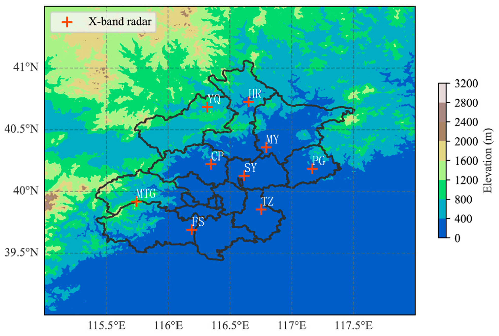
A relatively dense X-band dual-polarization weather radar network has been established in the Beijing metropolitan area. As of 2023, a total of nine X-band dual-polarization Doppler weather radars have been deployed in the region (Figure 1), effectively compensating for the detection blind zones of S-band radars in the cone of silence and at low altitudes (0.1–3 km) over long distances [26,27]. The network was constructed in two phases. In Phase I, five radars were deployed in densely populated urban districts, including Fangshan (FS), Tongzhou (TZ), Shunyi (SY), Changping (CP), and Miyun (MY), prioritizing the monitoring of severe convective weather in urban cores. In Phase II, additional radars were installed in Mentougou (MTG), Pinggu (PG), Huairou (HR), and Yanqing (YQ), filling the detection gaps in the western and northern mountainous areas. The average inter-radar spacing is approximately 48 km, leveraging the advantages of compact size, high spatial resolution, and flexible deployment.

2.2. Opposing RHI Calibration Method

The proposed networked X-band radar collaborative calibration approach establishes a dual-node cooperative observation between a reference radar and a radar under calibration. By exploiting the spatial overlap region formed by the opposing scanning patterns of the two radars, effective spatial matching data are screened and obtained.

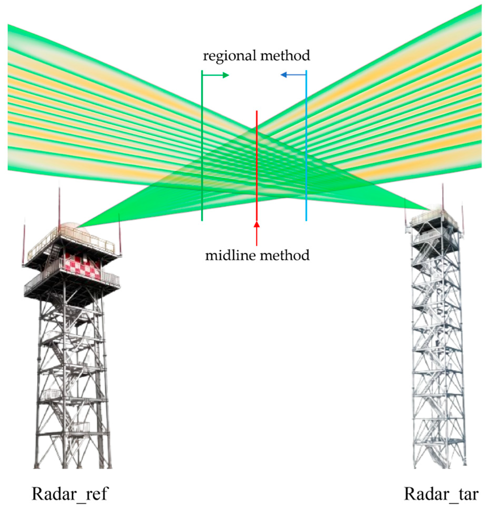
As illustrated in Figure 2, when the reference radar (Radar_ref) performs an RHI vertical profile scan along the azimuth toward the radar under calibration (Radar_tar), the latter is synchronously triggered to execute a corresponding RHI scan along the opposite azimuth. The scanning beams of the two radars thus form an overlapping region in space.

Since the two radars execute opposing RHI scans based on unified scheduling instructions (with a measured start-up observation error of less than 5 s), the temporal synchronization error is negligible. Therefore, the calibration accuracy depends primarily on the accuracy of spatial matching. The calibration process consists of three key steps:

• Establishing the reference benchmark. Within the radar network system, a radar that has undergone rigorous external calibration (e.g., metal sphere) and exhibits stable performance is selected as the reference radar. It should be noted that, due to airspace constraints, the radars in this study were calibrated using only the instrument-level method and the solar method, and the metal sphere method could not be performed for absolute calibration. Therefore, in the method validation of this study, it is assumed that the selected reference radar has undergone strict calibration. The adaptability and limitations of the proposed method are validated by analyzing the correlation coefficient, bias, and standard deviation of the paired data.
• Executing opposing RHI scans. The radar under calibration and the reference radar simultaneously perform opposing RHI scans. The elevation angle range of both radars is no less than 40°, and their scanning azimuth angles are oriented toward each other. Since both radars start scanning simultaneously, temporal synchronization is inherently achieved without requiring additional time registration processing. The spatial geometry of the scanning overlap region depends only on the inter-radar distance, the scanning azimuth angles, and the beamwidth.
• Bias calculation and calibration correction. Effective matching data are screened within the midline or regional spatial overlap, and the systematic bias of the radar under calibration is calculated using nearest-neighbor matching and statistical methods.

2.3. Bias Calibration Algorithm

After completing the RHI scans and data acquisition, data cleaning and quality control are performed (i.e., removing data with low correlation coefficients and low SNR), It should be noted that this study primarily validates the calibration performance under weak-to-moderate precipitation conditions, and therefore no attenuation correction algorithm was applied to the RHI scan data. Subsequently, a statistical distribution comparison is conducted for quantitative bias estimation. This study employs both the midline method and the regional method for calculation and comparison.

2.3.1. The Midline Method

The distance R between the reference radar and the radar under calibration is calculated. Within the spatial neighborhood on both sides of the vertical line at R/2, a 3 × 3 spatial window (comprising nine spatially adjacent points) is constructed by extending one step along both the elevation angle direction and the range bin direction, centered on the matching point [28]. The reflectivity factors of these nine points are arithmetically averaged, and this average value is used as the reflectivity factor of the matching point for subsequent bias calculation.

Specifically, after spatial matching at R/2 between the reference radar and the radar under calibration, the spatial indices corresponding to the k-th matching point pair are ($i_k^{\left(1\right)},j_k^{\left(1\right)}$) and ($i_k^{\left(2\right)},j_k^{\left(2\right)}$), where i represents the elevation layer index and j represents the range bin index. The 9-point averaged reflectivity factor ${\overline{z}}_k^{\left(m\right)}$ for this matching point in radar m (m = 1 for reference radar, m = 2 for radar under calibration) is defined as:

$${\overline{z}}_k^{\left(m\right)}={\displaystyle \frac{1}{N_{valid}}}{\displaystyle \sum _{u=-1}^1}{\displaystyle \sum _{v=-1}^1}{Z}^{\left(m\right)}(i_k^{\left(m\right)}+u,j_k^{\left(m\right)}+v)·L_{valid}(i_k^{\left(m\right)}+u,j_k^{\left(m\right)}+v)$$

(1)

where $L_{valid}(p,q)$ is the valid data indicator function, taking a value of 1 when the index $(p,q)$ is within the valid range and the corresponding reflectivity factor value is non-NaN, and 0 otherwise. $N_{valid}$ is the total number of valid points. When $N_{valid}<5$, indicating insufficient valid data within the window, the original single-point value at the center point is used.

2.3.2. The Regional Method

When the data samples in the midline region are limited or exhibit insufficient correlation, it is necessary to simultaneously employ a regional statistical method using a larger dataset as a comparative reference. This method is not confined to matching points near the radar center; instead, it incorporates the entire spatially constrained overlap region into the statistical scope, forming a substantial data sample.

Spatial Overlap Region Selection

Let the horizontal distance between the reference radar and the radar under calibration be R, with the reference radar located at the starting position and the radar under calibration at distance R, and the beamwidth be θ. Selecting a target height H, the slant-range beam broadening at horizontal position x is:

$$W_{\left(x\right)}=\sqrt{x^2+H^2}·\theta$$

(2)

Taking the beam broadening cross-section at the center distance R/2 as the reference:

$$W_{mid}=\sqrt{{\left({\displaystyle \frac{R}{2}}\right)}^2+H^2}·\theta$$

(3)

The beam cross-coverage ratio η(x) is defined as the ratio of the smaller beam broadening cross-section at the current position to the reference cross-section:

$${\mathsf{\eta }}_{\left(x\right)}={\displaystyle \frac{min\left[\sqrt{x^2+H^2}·\theta ,\sqrt{{\left(R-x\right)}^2+H^2}·\theta \right]}{\sqrt{{\left(\frac{R}{2}\right)}^2+H^2}·\theta }}$$

(4)

Setting a cross-coverage ratio threshold t (0 < t < 1), requiring η(x) ≥ t, the horizontal interval satisfying this condition can be solved as:

$$\left[R_1,R_2\right]=\left[\sqrt{t^2\left({{\displaystyle \frac{R}{4}}}^2+H^2\right)-H^2},R-\sqrt{t^2\left({{\displaystyle \frac{R}{4}}}^2+H^2\right)-H^2}\right]$$

(5)

An excessively low cross-coverage ratio would result in insufficient matching samples, while an excessively high ratio would overly restrict the effective interval. Within this interval, the beam broadening of both radars at any position is no less than t times the reference broadening at the midpoint, thereby ensuring sufficient beam cross-coverage and data comparison reliability.

Spatial Data Optimal Matching

After determining the target scanning overlap region Ω = [R₁, R₂], the nearest-neighbor search algorithm is employed to establish a one-to-one correspondence between data points from the reference radar and the radar under calibration. To balance matching accuracy while maximizing the utilization of valid data points, this study introduces the matching efficiency metric, defined as the ratio of actual matched point pairs to the theoretical maximum:

$$E={\displaystyle \frac{N_{matched}}{\mathrm{m}\mathrm{i}\mathrm{n}(N_{ref},N_{cal})}}·100\%$$

(6)

where $N_{matched}$ is the number of actual matched point pairs satisfying the tolerance conditions, $N_{ref}$ and $N_{cal}$ are the numbers of valid data points in the overlap region for the reference radar and the radar under calibration, respectively, and the theoretical maximum number of matched pairs is the smaller of the two.

To determine the tolerance parameters that maximize matching efficiency, a traversal search is performed for different horizontal tolerances δh (e.g., 25 m, 30 m, 37.5 m) and vertical tolerance scaling factors α (e.g., 1/3, 1/2, 2/3). Vertically, since the elevation step of the RHI scan is 0.1° and the vertical spacing between adjacent elevation angles increases with distance, a distance-adaptive tolerance strategy is adopted [29]. Specifically, at horizontal distance L, the simplified vertical resolution for a 0.1° elevation step is approximately:

$$∆h\left(L\right)=\alpha ·L·\sin \left(0.1°\right)$$

(7)

where α is the vertical tolerance scaling factor. By comparing the matching efficiency and correlation coefficient under different parameter combinations, the parameter set yielding the highest matching efficiency is selected as the final matching scheme. This configuration effectively avoids the problem of a single data point matching multiple neighboring points due to excessive tolerance, while retaining sufficient matched point pairs for subsequent bias statistical analysis.

2.3.3. Quantitative Bias Calculation

First, the linear correlation between valid data point pairs $\left(Z_{1,i},Z_{2,i}\right)$ after spatial matching is calculated using:

$$r={\displaystyle \frac{{\sum }_{i=1}^n\left(Z_{1,i}-Z_1\right)\left(Z_{2,i}-Z_2\right)}{\sqrt{{\sum }_{i=1}^n{\left(Z_{1,i}-\overline{Z_1}\right)}^2}·\sqrt{{\sum }_{i=1}^n{\left(Z_{2,i}-\overline{Z_2}\right)}^2}}}$$

(8)

where n is the total number of valid matched point pairs, and $\overline{Z_1}$ and $\overline{Z_2}$ are the means of the matched data from the reference radar and the radar under calibration, respectively. A value of r closer to 1 indicates stronger consistency between the observations of the two radars. The correlation coefficient is adopted for performance comparison based on the following considerations: according to Cohen’s (1988) effect size criteria, r ≥ 0.8 represents a large effect size [30]. In related studies based on 98,226 matched samples, the correlation coefficient between space-based and ground-based radars reached 0.87, validating the reasonableness of this threshold [31].

Next, the bias for each matched pair is calculated:

$$∆Z_i=Z_{2,i}-Z_{1,i}$$

(9)

Then, the mean and standard deviation of the bias are computed:

$$\overline{∆Z}={\displaystyle \frac{1}{N}}{\displaystyle \sum _{i=1}^N}∆Z_i$$

(10)

$${\sigma }_{∆Z}=\sqrt{{\displaystyle \frac{1}{N-1}}{\displaystyle \sum _{i=1}^N}{\left(∆Z_i-\overline{∆Z}\right)}^2}$$

(11)

Studies have shown that inter-radar bias assessment is influenced by spatiotemporal overlap. By setting reasonable thresholds and screening optimal comparable datasets, matching quality and bias estimation reliability can be improved. In the lower Yangtze River region, after applying a screening comparison method to seven S-band radars, the average reflectivity factor difference was reduced from 1.8 dB to 0.5 dB, with differences between any two radars being less than 1.0 dB [32]. However, X-band radars exhibit varying calibration performance under different precipitation conditions due to issues such as beam broadening, severe attenuation, and low sensitivity [33,34,35]. Therefore, it is necessary to validate calibration stability under uniform precipitation conditions, the impact of spatial echo inhomogeneity on bias estimation, and the number of valid matching points and statistical reliability under weak echo conditions. The applicability of the proposed method will be evaluated through case studies in Section 3.

3. Results

3.1. Overview of Experimental Design

To validate the effectiveness of the collaborative calibration method using opposing RHI scans, this study selected data from opposing RHI scan cases conducted under various precipitation conditions from July 2023 to September 2025. Based on the echo characteristics and the spatial continuity of the vertical profiles, the experimental data were categorized into three types: stratiform precipitation (homogeneous/inhomogeneous echoes), scattered precipitation (homogeneous/inhomogeneous echoes), and weak cloud (reflectivity factor < 15 dBZ). A total of 59 RHI calibration cases were conducted. Excluding 1 case with incomplete scan data, 58 cases were used for analysis. For each experiment, both the midline method and the regional method were employed for data matching and bias calculation, with a comparative analysis of the calibration effectiveness of the two methods. A summary of the experimental design is provided in

Table 1. Summary of Opposing RHI Calibration Cases by Precipitation Type.

Precipitation Type	Echo Characteristics	Example Radar Pairs	Number of Cases
Stratiform	Homogeneous	MY-HR, TZ-FS, SY-FS, SY-CP, CP-SY, CP-TZ, CP-FS	34
	Inhomogeneous	FS-TZ	3
Scattered	Homogeneous	CP-FS, FS-TZ	6
	Inhomogeneous	SY-FS, TZ-FS, MY-TZ, SY-CP	6
Weak Cloud	Homogeneous	TZ-FS, CP-TZ, TZ-SY, SY-TZ	10

.

3.2. Calibration Cases Under Different Precipitation Types

Due to space constraints, this paper presents only 25 representative cases for illustration, but all data were used in the summary of experimental results to assess the stability and adaptability of the methods under different echo types.

3.2.1. Under Stratiform Precipitation Conditions

Homogeneous Echo Conditions

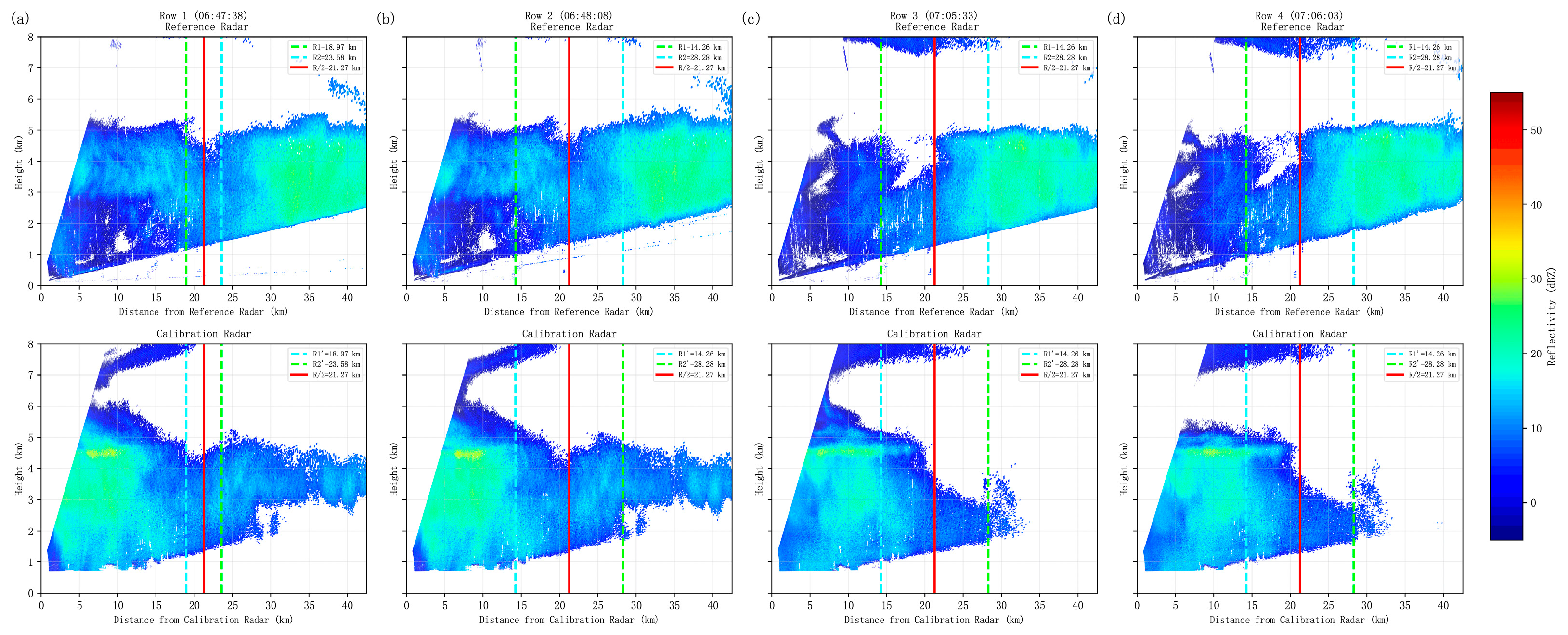
To better validate the impact of echo intensity and large bias on the calibration method under homogeneous echo conditions, a total of ten valid cases from three processes were selected for verification, covering multiple radar pairs, including MY–HR, TZ–FS, SY–FS, CP–FS, and CP–TZ. Taking the example of four consecutive RHI scans from the MY–HR radar pair on 5 September 2025, the echoes during this period were homogeneous but weak, with a maximum reflectivity factor not exceeding 35 dBZ (Figure 3).

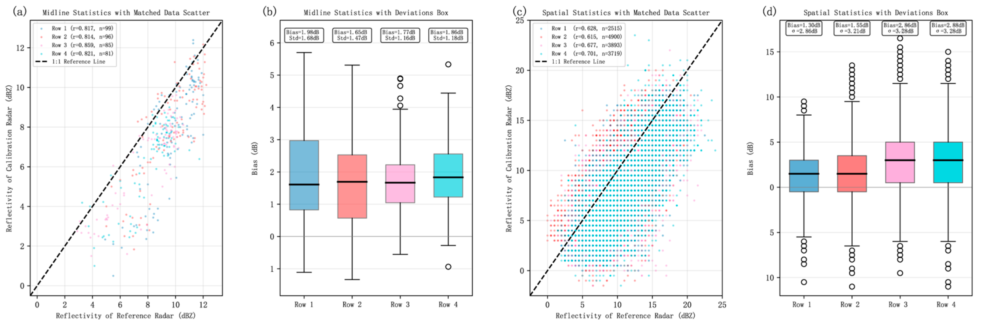
Figure 4 shows the comparison of matching results for the four RHI scans of MY and HR. Due to the observation geometry of the dual radars, echoes were weaker near the reference radar and weaker near the far end of the radar being calibrated. Weak echoes at the far end of the radar being calibrated often fell below the sensitivity threshold, preventing valid observation data from being obtained. Using the midline method, the correlation coefficients stabilized between 0.814–0.859 (n = 81–99), with a maximum fluctuation of no more than 0.05 within the half-hour time window. The mean bias fluctuated between 1.65–1.98 dB, and the standard deviation decreased from 1.68 dB in the first scan to approximately 1.18 dB, indicating an improvement in matching quality with consecutive scans. In contrast, after matching using the regional method, the correlation coefficients were only 0.615–0.701 (n = 2515–4900). Both the bias (1.30–2.88 dB) and standard deviation (2.86–3.28 dB) increased with successive calibration scans, indicating that under homogeneous but weak echo conditions, the regional method was limited by low signal-to-noise ratio (SNR) and insufficient sensitivity [36].

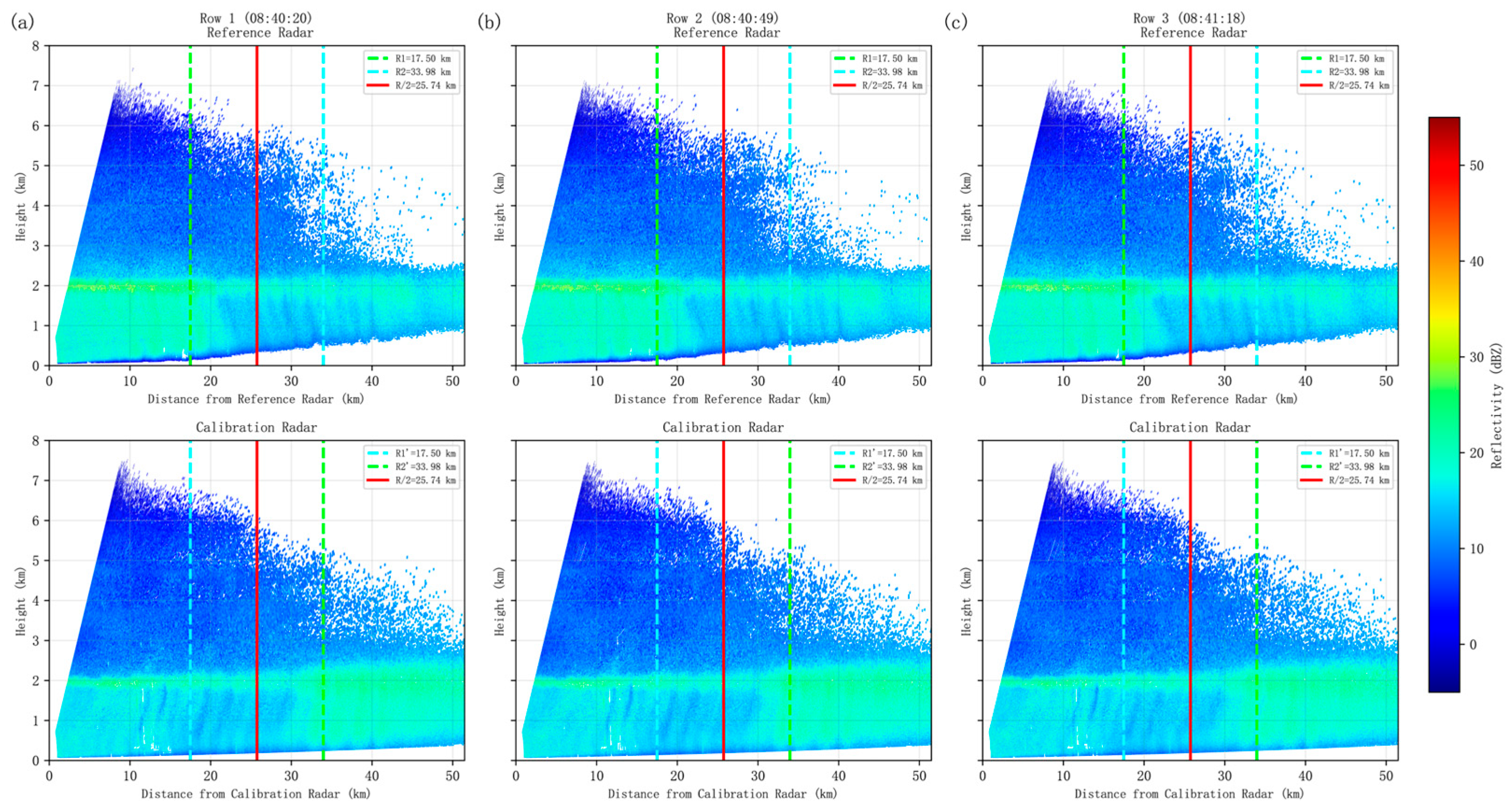
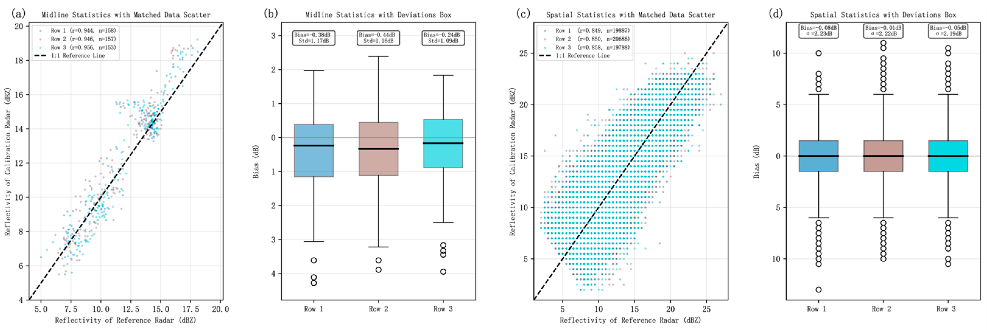
From 08:40 to 08:41 on 9 May 2025, radars TZ and FS performed three consecutive RHI calibration scans. The corresponding reflectivity factor was higher than that in the previous case, as shown in Figure 5, exhibiting characteristics typical of stratiform cloud precipitation. Figure 6 shows the comparison of the two matching methods. Using the midline method, the matched sample sizes for each scan were approximately 153–158. The correlation coefficients were significantly higher, at 0.944–0.956. The mean biases ranged from −0.24 to −0.44 dB, and the standard deviation decreased from 1.16 dB (06:47) to 1.09 dB (07:05), showing slight improvement as the system stabilized over the time window. Using the spatially constrained regional method, the matched sample sizes were approximately 1.98 × 10⁴–2.07 × 10⁴, with correlation coefficients of 0.849, 0.850, and 0.858. The bias box plots indicated very small mean biases (−0.08, −0.01, −0.05 dB), and standard deviations were stable between 2.19–2.23 dB.

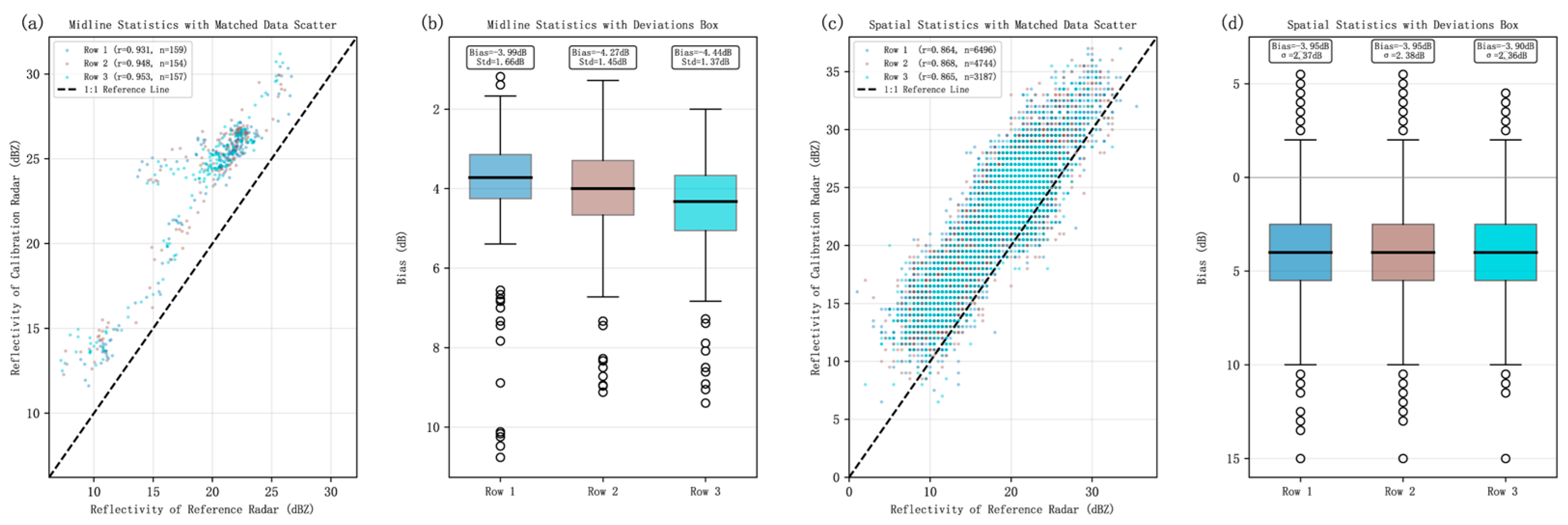
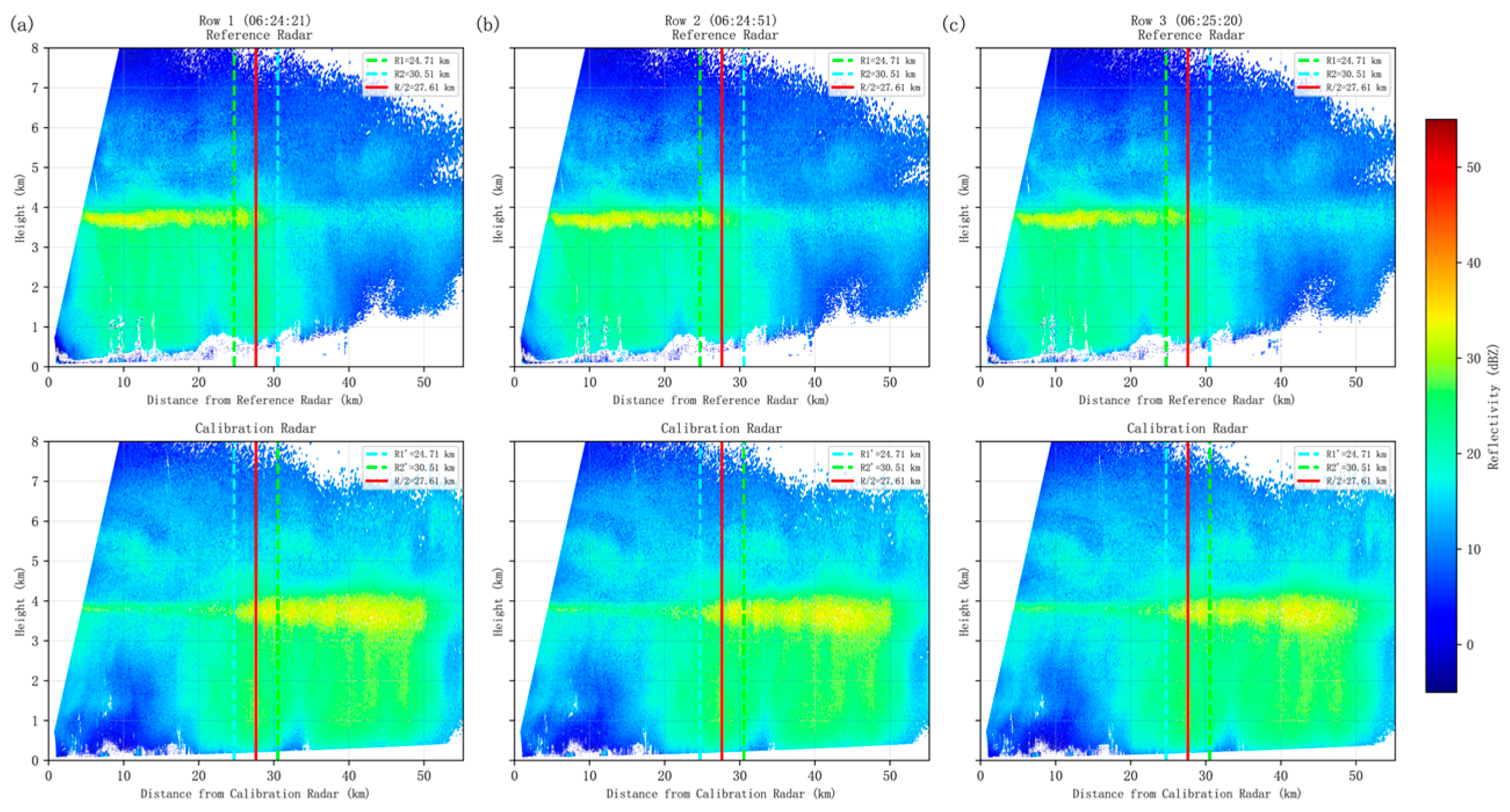
On 24 May 2024, radars CP and FS performed three consecutive calibration scans (Figure 7). Figure 8 shows the matching results for the two methods. Using the midline method, the matched sample sizes for each scan were approximately 154–159, with correlation coefficients of 0.948, 0.953, and 0.931. The mean biases were −4.27, −4.44, and −3.99 dB, showing close agreement with a systematic bias of approximately −3.95 dB. The standard deviations were 1.45, 1.37, and 1.66 dB, indicating tight dispersion and stable matching quality across the three scans. In contrast, using the regional method, the matched sample sizes were substantially larger (4744, 3187, and 6496), with correlation coefficients of 0.868, 0.865, and 0.864, respectively. The mean bias was approximately −3.95 dB, and the standard deviations were 2.38, 2.36, and 2.37 dB, showing high consistency across scans but slightly higher dispersion than the midline method. In this example, both methods yielded highly consistent bias estimates for the two radars (approximately −4.0 dB), necessitating a comprehensive calibration of the radars before bias correction. Multiple cases indicate that under conditions with a horizontally layered echo structure, both methods can effectively calibrate the biases between radar systems.

In multiple uniform stratiform cloud cases, both echo intensity and the bias of the radar being calibrated had minimal impact on the calibration methods. The two matching methods demonstrated good calibration consistency and were capable of meeting operational calibration needs. The midline method, which focused on the vicinity of the midline, achieved a correlation coefficient above 0.90, albeit with a smaller sample size. In contrast, the regional method, leveraging a large sample size, provided a statistically robust estimate of the overall bias; however, due to low signal-to-noise ratio and limited sensitivity in the overlapping area, its correlation coefficient was slightly lower and its dispersion was larger. In practical applications, the choice between the two methods can be optimized based on the specific objective of prioritizing “overall statistics” or “midline analysis”.

Inhomogeneous Echo Conditions

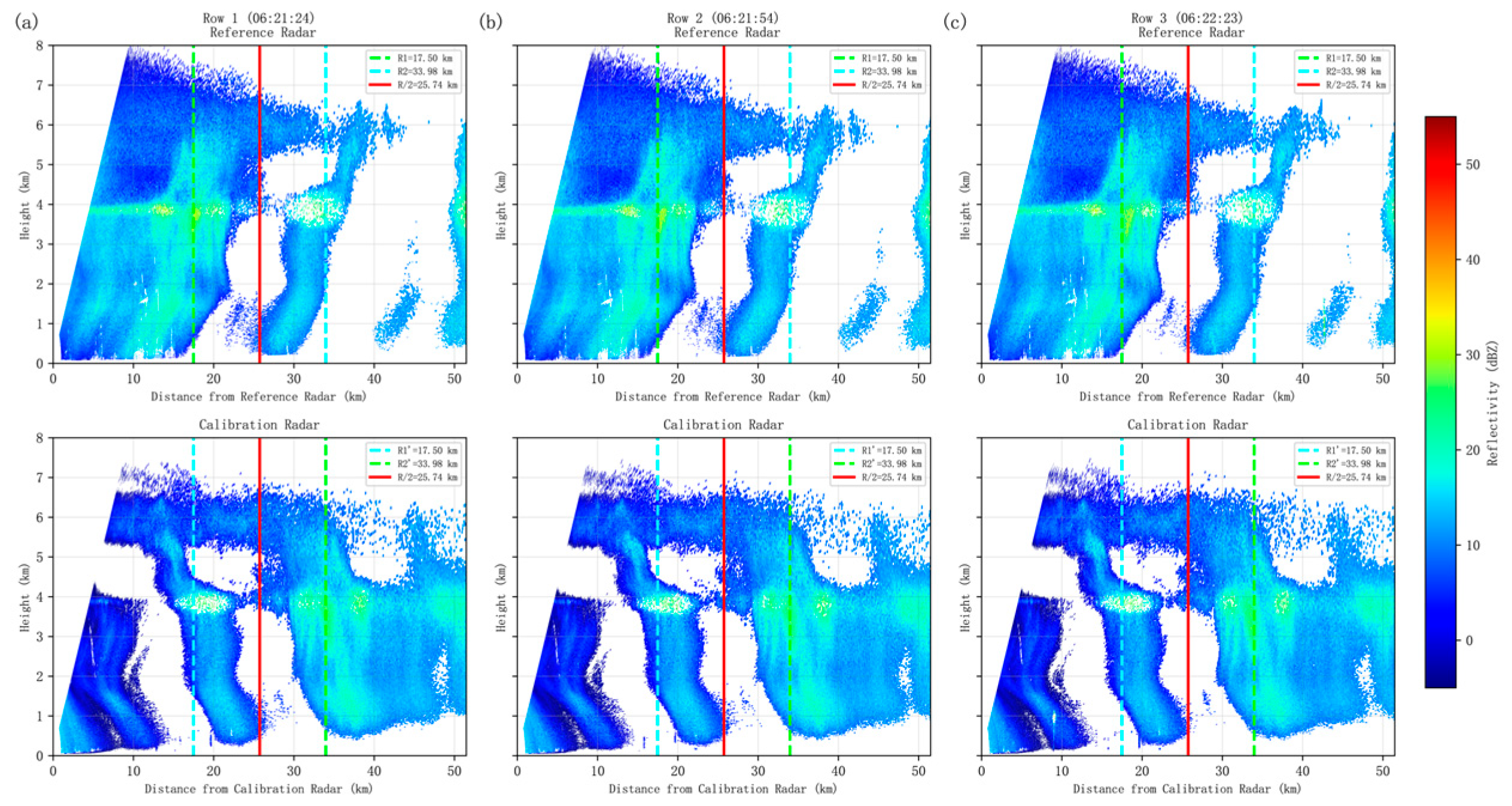
Under conditions of inhomogeneous echoes in stratiform precipitation, a total of 6 valid cases were completed. Taking the example of synchronized RHI calibration scans between FS and TZ on 24 May 2024, the RHI vertical profile showed discontinuities near the midline. The reference radar echo exhibited an inhomogeneous spatial distribution biased to the left within the matching area (Figure 9).

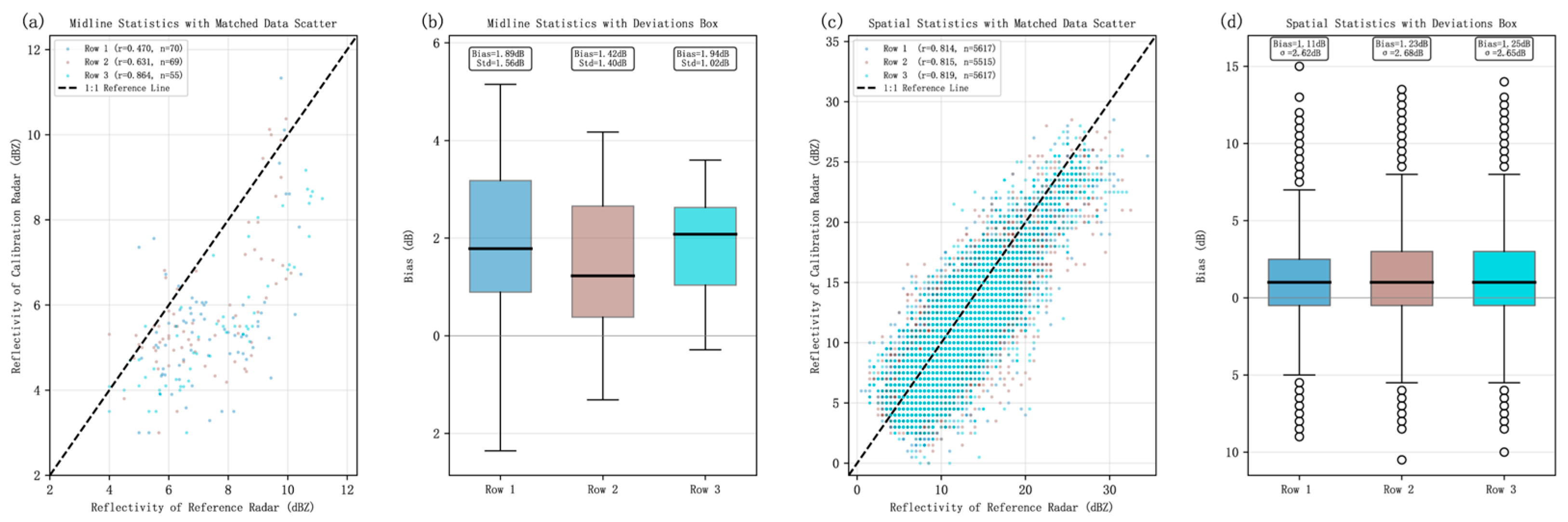
Due to the inhomogeneous structure, the overlapping matching areas of the three RHI calibration cases showed an inhomogeneous distribution, limiting the number of continuous samples available for comparison within the matching zone. This had a certain impact on the subsequent comparative evaluation of the methods. Figure 10 shows the comparison of the two matching methods. Extracting matching points along the midline vicinity of the overlapping area yielded sample sizes of only 55–70 per scan, significantly fewer than the 154–159 observed in homogeneous cases. Under the midline method, the correlation coefficients fluctuated considerably: 0.470, 0.632, and 0.864, with the first two scans showing significantly low correlations. The mean biases were 1.89, 1.42, and 1.94 dB (indicating a systematic overestimation by the radar being calibrated), and the standard deviations were 1.56, 1.40, and 1.02 dB. In contrast, using the regional method, the matched sample sizes were 5617, 5515, and 5617, with correlation coefficients of 0.814, 0.815, and 0.819. The mean biases ranged from 1.11 to 1.25 dB, and the standard deviations were 2.62, 2.68, and 2.65 dB, showing a slight increase in dispersion compared to cases with homogeneous echoes.

This case illustrates the differential impact of inhomogeneous echoes on the two matching methods. The midline method was more significantly affected: the intermittent distribution of echoes near the midline reduced the effective sample size to 55–70. Its correlation coefficient was only 0.470 in the first scan, indicating a significant decline in reliability when samples were extremely sparse. Its correlation coefficient only increased to 0.864 in the third scan when echo continuity improved and sample validity increased. However, the regional method, by virtue of its wider spatial window, retained sufficient samples (n ≈ 5.6 × 10³) and maintained a stable correlation coefficient around 0.81. Overall, under inhomogeneous echo conditions, the robustness of the regional method was superior to that of the midline method. However, both methods struggled to achieve the calibration accuracy observed in homogeneous echo cases. In practical applications, it is necessary to assess the validity of matched samples based on echo continuity.

3.2.2. Under Scattered Precipitation Conditions

Scattered precipitation includes two sub-types, homogeneous (continuous) and inhomogeneous (discontinuous) spatial echo distribution in the vertical profile. Slightly different from stratiform precipitation, the echo intensity and gradient variations are somewhat larger for scattered precipitation.

Homogeneous Echo Conditions

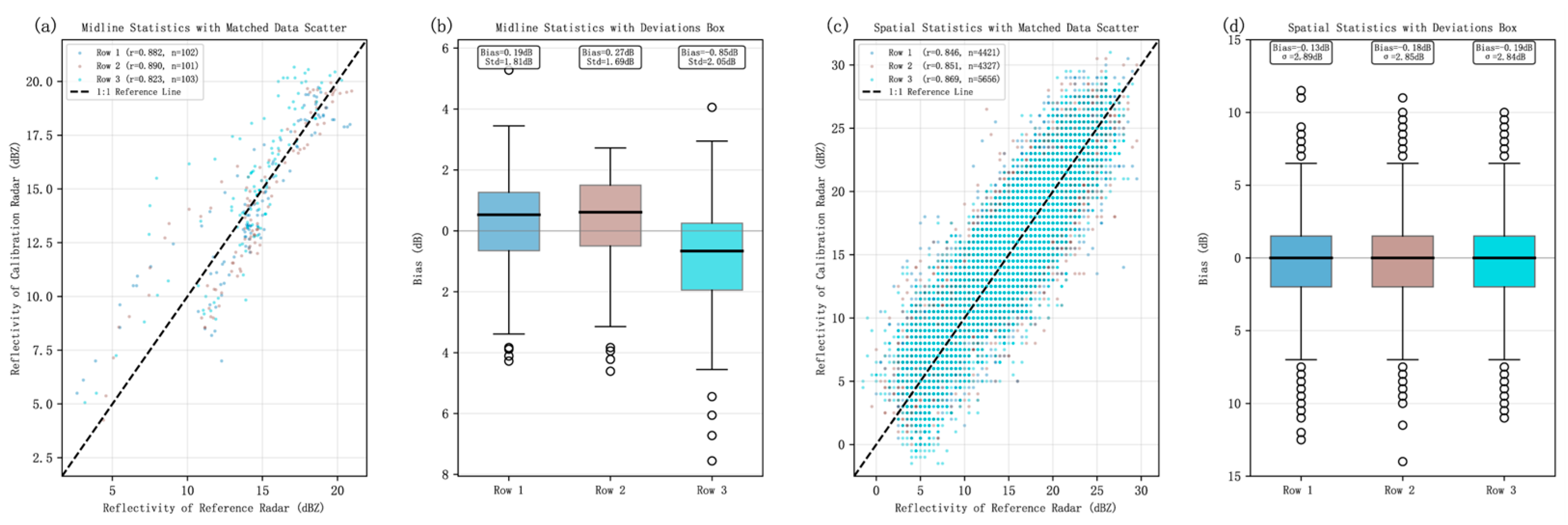
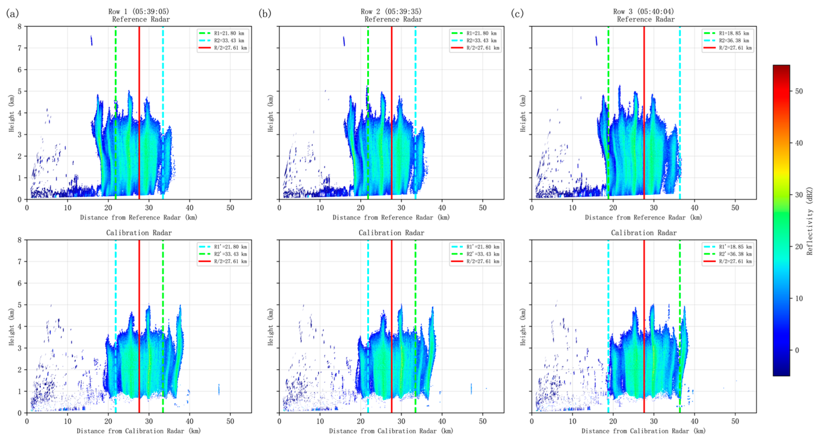
On 25 July 2024, scattered precipitation occurred in the Beijing area. Calibration cases were conducted using relatively homogeneous echoes near the midline of radars FS and CP. A total of three sets of RHI reflectivity factor data were collected (Figure 11). Figure 12 shows the comparison of the two matching methods.

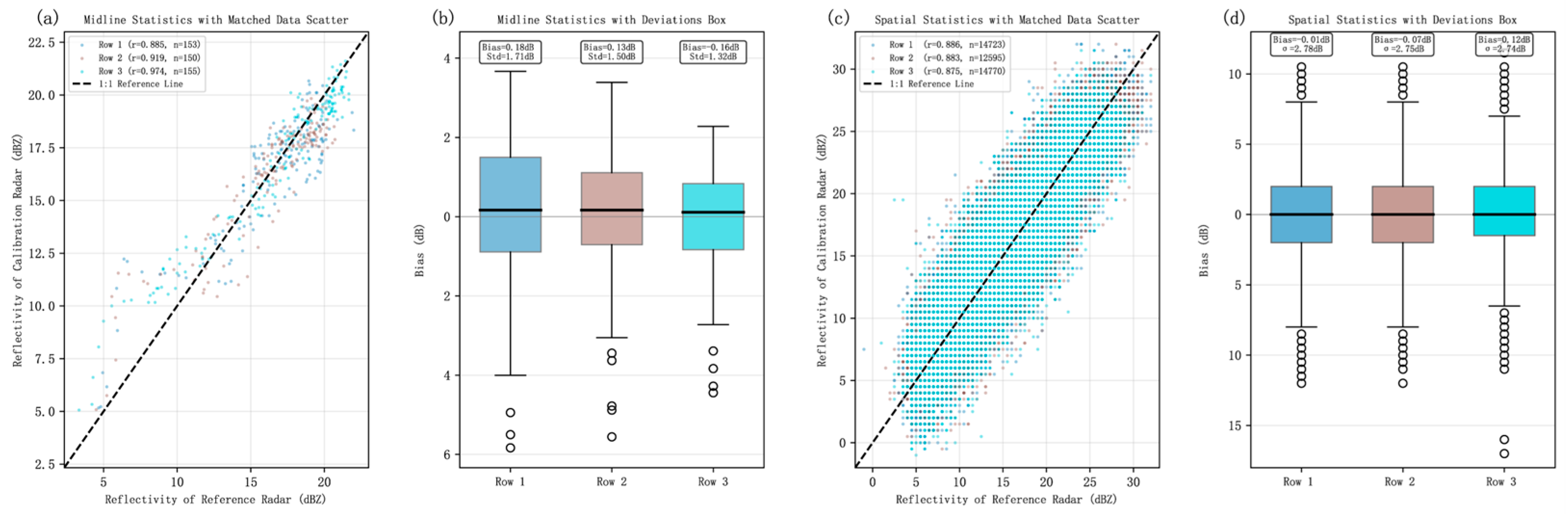
In this case, using the midline method, the sample sizes for each scan were approximately 101–103, with correlation coefficients of 0.882, 0.890, and 0.823. The mean biases were 0.19, 0.27, and −0.85 dB, and the standard deviations were 1.81, 1.69, and 2.05 dB. In contrast, using the regional method, the sample sizes were 4421, 4327, and 5656, with correlation coefficients of 0.846, 0.851, and 0.869. The mean biases were near zero (−0.13, −0.18, −0.19 dB), and the standard deviations were 2.89, 2.85, and 2.84 dB. The correlation coefficients of both methods generally remained around 0.85, indicating overall stability.

With continuous echo filling, both methods achieved good calibration consistency. The midline method, applied under homogeneous scattered precipitation, yielded sample sizes of approximately 100, correlation coefficients ranging from 0.83 to 0.87, and a dispersion of 1.7–2.2 dB. In contrast, the regional method, leveraging its large sample size, provided a statistically robust overall estimate, with correlation coefficients of approximately 0.85 and biases near zero (−0.13 to −0.19 dB). Overall, the bias estimates from both methods were in close agreement, indicating reliable calibration quality under conditions of continuous echo filling. However, it should be noted that the midline method’s smaller sample size may limit its robustness under highly heterogeneous echo conditions.

Inhomogeneous Echo Conditions

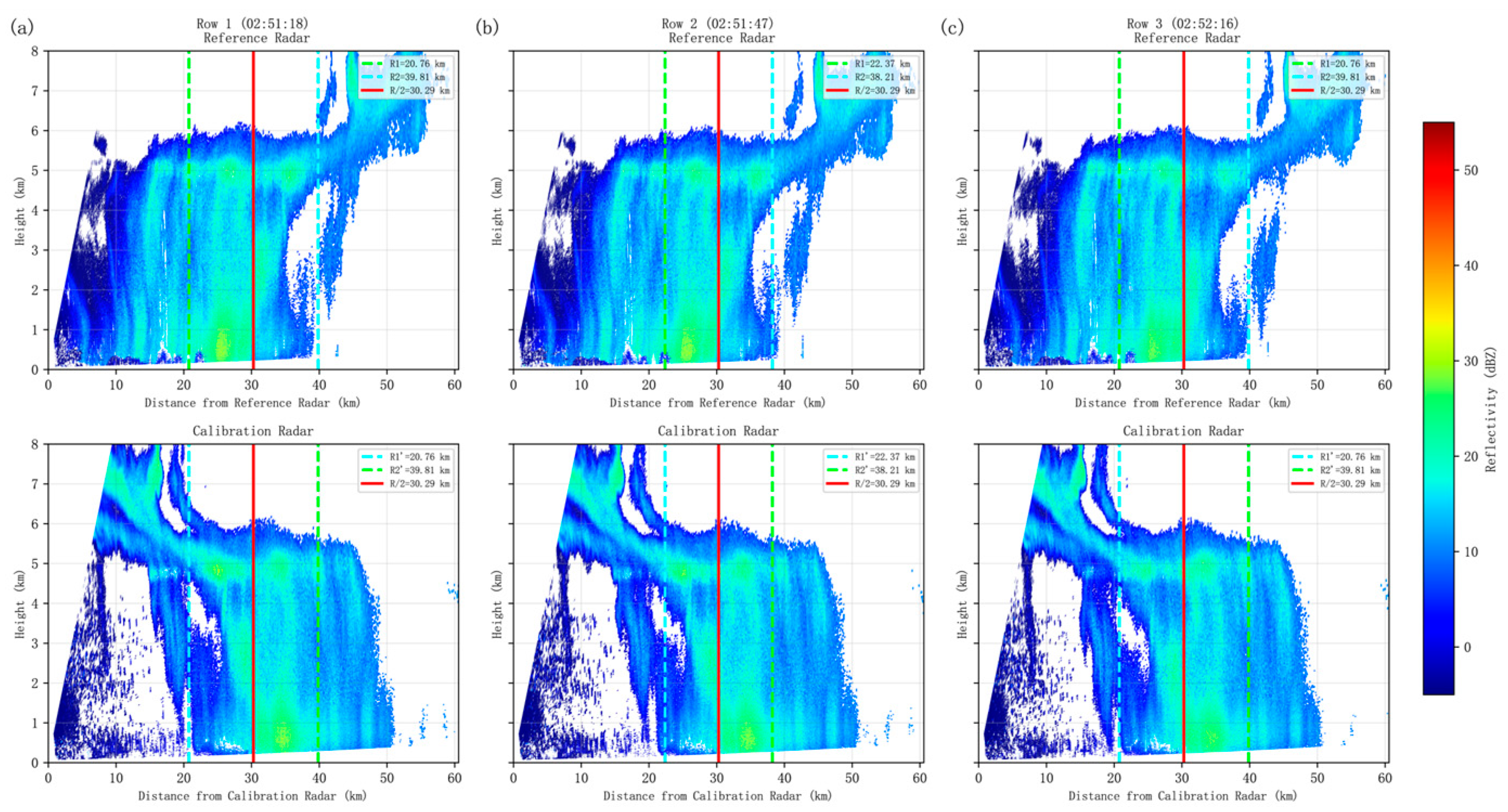
This section focuses on the impact of spatially asymmetric echoes (biased to left/right) on the applicability of the two matching methods. Using the example of three consecutive RHI scans from radars FS and SY on 25 July 2024, during this scattered precipitation event, the reference radar echo was generally biased to the right, while the radar being calibrated observed the same echo from the far end (Figure 13). Figure 14 shows the matching results.

From the matching results, the geometric offset did not impact the calibration quality. Using the midline method, the matched samples were about 150–155, with even higher correlation coefficients (0.885, 0.919, 0.974), mean biases of −0.16 to −0.18 dB, and standard deviations of 1.32–1.71 dB. In contrast, the regional method accumulated approximately 12,595–14,770 matched samples within the optimal matching interval, achieving correlation coefficients of 0.875–0.886, mean biases of −0.07 to 0.12 dB, and standard deviations of about 2.74–2.78 dB. Both methods showed biases near zero and moderate dispersion, indicating that as long as the main echo body is coherent and discernible, echo asymmetry does not significantly affect radar calibration.

This result suggests that the dominant factor constraining calibration accuracy is not the “spatial position” of the echoes but their “continuity” within the matching area. Although this case involved scattered precipitation with an inhomogeneous structure, the echoes within the matching interval were coherent and without discontinuous gaps; consequently, the performance of the midline method (with correlation up to 0.974) and the regional method remained comparable to that of homogeneous cases. In contrast, for the inhomogeneous case involving the same radar pair on 24 May 2024, discontinuities in the vertical profile reduced the midline sample size sharply to 55–70, and its correlation coefficient dropped to as low as 0.470, while the regional method also showed increased bias variability. A comparison of these two cases shows that geometric asymmetry is tolerable when echoes are coherent; the true factor that degrades matching quality is the discontinuity of echoes within the region.

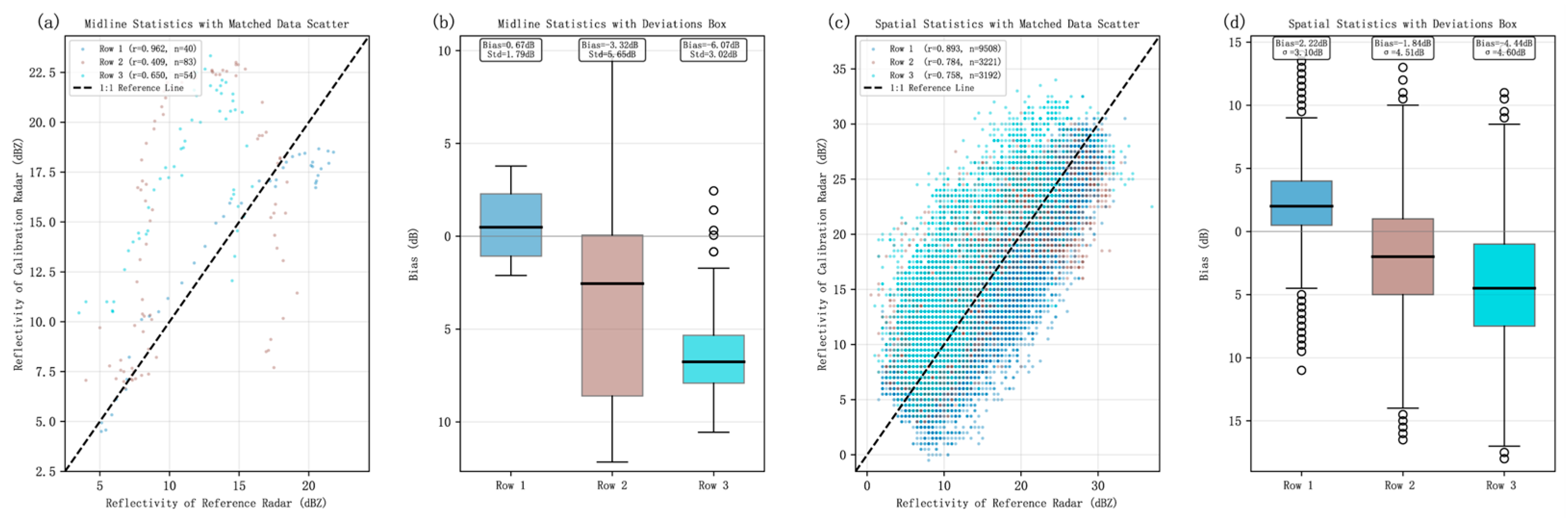
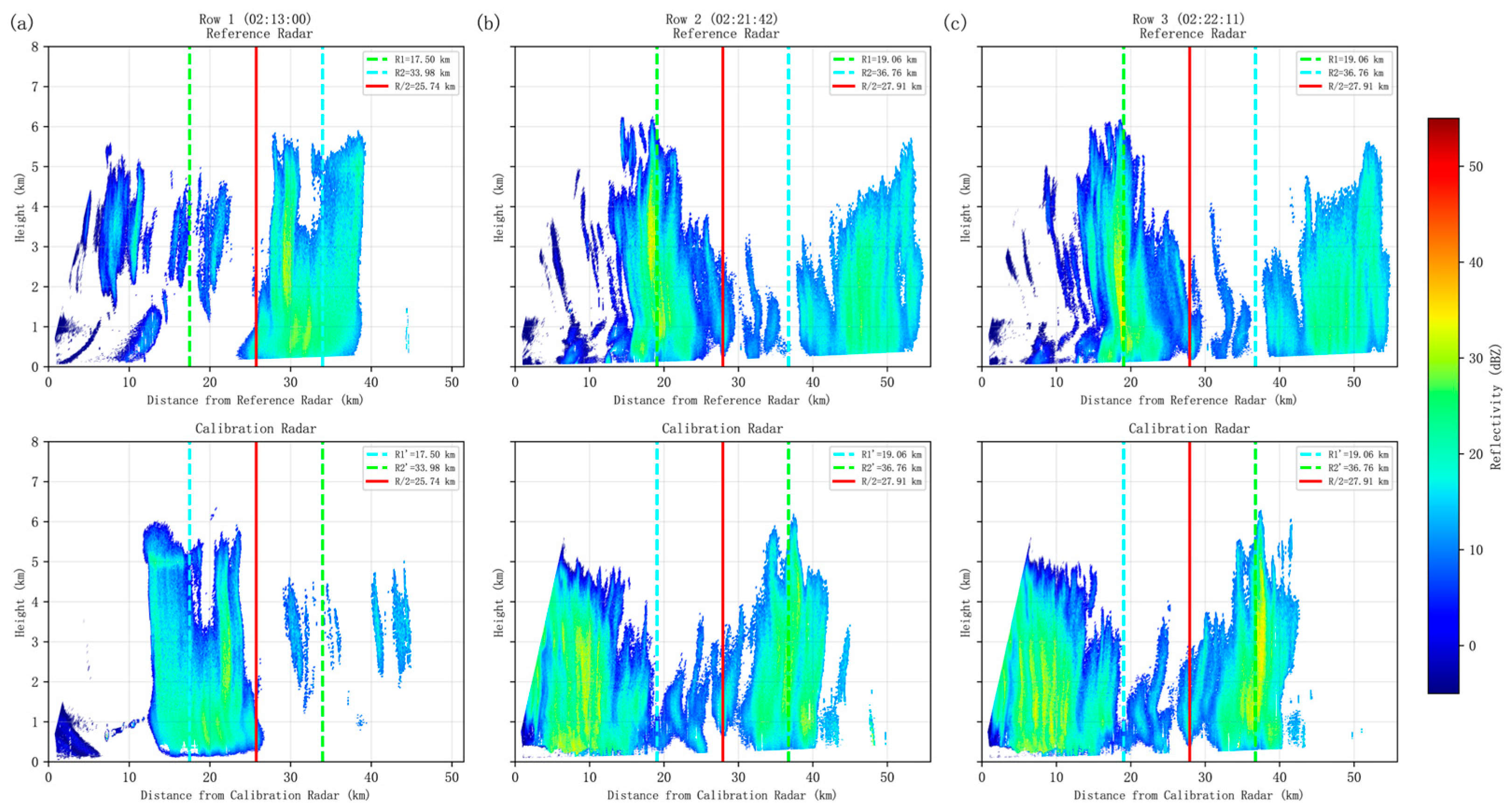
Multiple cases on 9 September 2024 further demonstrated the quality differences between the matching methods under inhomogeneous echo conditions (Figure 15), with corresponding matching results shown in Figure 16. Using opposing RHI scans, two sets of calibration data were acquired within the same time period: FS and TZ completed one paired scan at 02:13, and TZ and MY completed two consecutive scans at 02:21 and 02:22.

For the first set of echoes, although the correlation coefficients of both methods exceeded 0.85, the midline method matched only 40 echo points, leading to significant differences in bias and standard deviation between the two methods, which made it difficult to determine which was more accurate. For the second set of echoes, the consistency of the midline method decreased significantly: its correlation coefficients dropped to 0.409 and 0.650, biases were −3.32 dB and −6.07 dB, respectively, and the standard deviation reached 5.65 dB at 02:21. In contrast, for the regional method, the correlation coefficient dropped from 0.784 to 0.758, the bias expanded from −1.84 dB to −4.44 dB, and the standard deviation increased to 4.60 dB; its degradation was comparatively less severe. The divergence between the two methods in the two scenarios confirmed their inherent differences in robustness. The midline method, which uses very few samples from the midline vicinity, is highly sensitive to echo continuity; once matching points near the midline shift or jump due to echo movement, its correlation coefficient drops sharply. However, the regional method, relying on the average of a large sample of voxels, provides a smoothing buffer against local echo fluctuations, thus maintaining a correlation coefficient above 0.75 even in degraded scenarios. In summary, compared to spatial position offset, echo continuity is the primary factor limiting the effectiveness of the midline method; the regional method sacrifices some correlation for stability in terms of standard deviation.

3.2.3. Under Weak Cloud Conditions

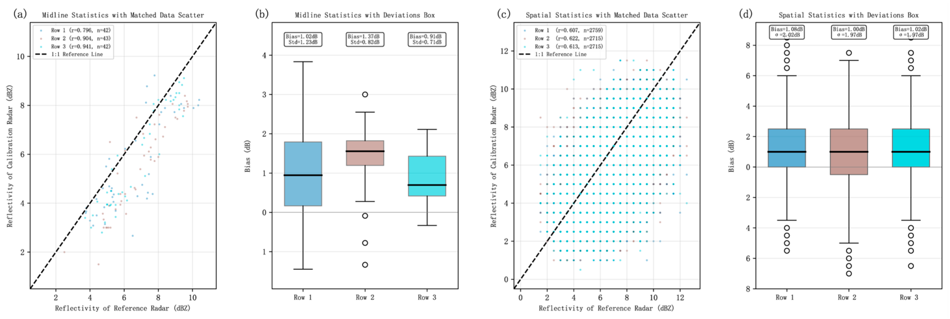
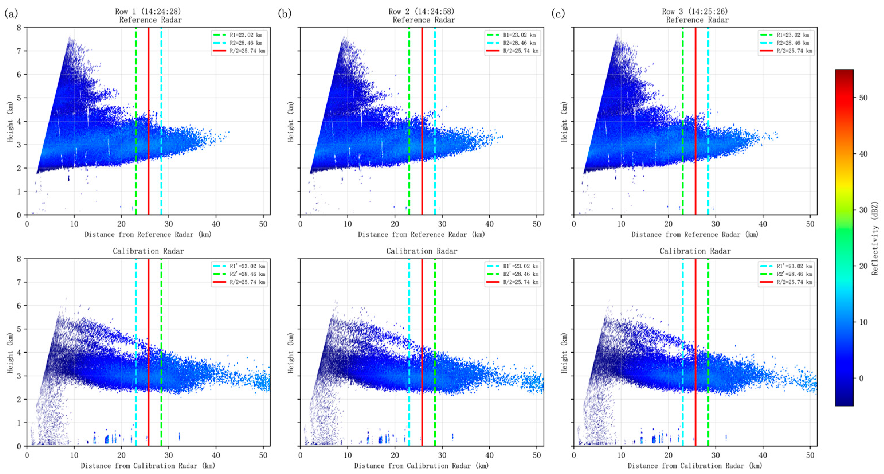
Under weak cloud conditions, taking the example of three consecutive RHI scan calibration cases between FS and TZ on 4 February 2024 (Figure 17), Figure 18 shows the comparison of results from the two matching methods.

From the scatter distribution, the points from the midline method are relatively concentrated, whereas those from the regional method show almost no clustering trend and are highly dispersed. In this low-SNR scenario, the correlation of the two methods was the reverse of that observed in strong-echo cases. Using only approximately 42 midline neighborhood points, the midline method achieved markedly higher correlation coefficients (0.796, 0.904, and 0.941), which increased as the echoes became more stable, and its standard deviation decreased from 1.23 dB to 0.71 dB. In contrast, although the regional method relied on a large sample size (n ≈ 2715–2759), its correlation coefficients were only 0.607, 0.622, and 0.613. The mean biases of both methods were positive (midline method: 1.02 to 1.37 dB; regional method: ≈1.0 dB, σ ≈ 2.0 dB).

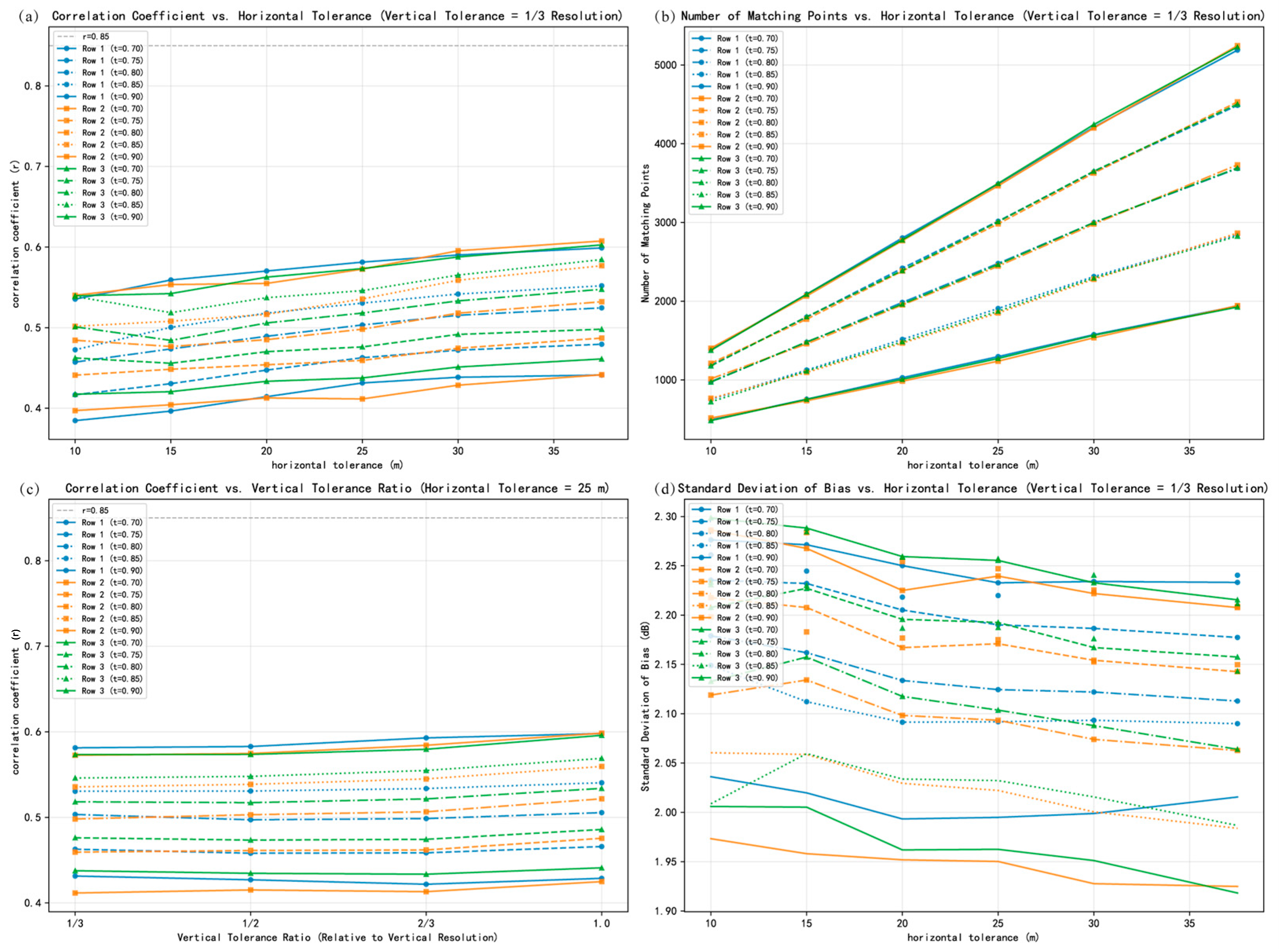
This case demonstrates that under weak-echo conditions, the averaging of a large sample is diluted by low-SNR noise, causing the correlation of the regional method to be inferior to that of the midline method, which focuses on the high-SNR midline points. Therefore, neither method is consistently superior or more accurate than the other, and their respective applicability ranges should be further evaluated using matched data. To this end, sensitivity tests on matching tolerance parameters were conducted based on three sets of RHI scan calibration data (Rows 1–3), using the beam cross-overlap ratio t (0.70–0.90) of the two radars as a screening condition for the validity of paired points. The results of these tests are presented in Figure 19, which evaluates the impact of data matching parameters on the consistency calibration of dual-radar RHI observations.

As shown in Figure 19a, with the vertical tolerance fixed at 1/3 of the vertical resolution, the correlation coefficients showed a slow upward trend as the horizontal matching tolerance increased (10–35 m). The correlation coefficients for all pairs were maintained at a relatively low level (r < 0.63), with the maximum value of 0.622 observed for Row 2 under t = 0.9 and horizontal tolerance = 37.5 m, indicating weak correlation between the two RHI datasets under the current matching strategy. Conversely, the number of matched points increased approximately linearly with the horizontal tolerance (Figure 19b), rising from about 500 points to over 7500 points, with the most significant increase observed for the second scan pair.

Further examining the vertical dimension, with a horizontal tolerance fixed at 25 m, the correlation coefficient showed only a weak increasing trend as the vertical tolerance ratio increased from 1/3 to 1.0 (Figure 19c), indicating that the vertical tolerance had a relatively limited impact on the correlation coefficient. Increasing the beam cross-overlap ratio t led to a slight improvement in correlation. Bias analysis (Figure 19d) showed that the standard deviation of the bias ranged between 1.9–2.4 dB, with small variations with horizontal tolerance. The first scan pair exhibited the smallest and most stable bias (about 1.92–2.37 dB), while the second scan pair showed a relatively larger bias (about 2.0–2.36 dB).

Overall, the choice of horizontal matching tolerance represents a key trade-off between the coverage of matched points and the correlation coefficient. A larger tolerance increases the density of matched points but weakens the correlation, while the stability of the bias is insensitive to tolerance changes. Increasing the beam cross-overlap ratio t helps improve correlation but restricts the number of matched points. The parameter sweep results for the three scans showed that the correlation coefficient was relatively low across all 120 parameter combinations, with a maximum value of only 0.622. This indicates that under weak echo conditions, due to the lack of significant echo texture structure, the region-based matching algorithm essentially fails. However, the midline method achieved correlation coefficients of 0.796–0.941 and standard deviations of only 0.71–1.23 dB, the lowest among all tests. This seemingly contradictory result reveals that under weak echo conditions, the regional method exhibits a significant drop in correlation because it includes a large number of low-SNR regions. In contrast, the midline method, by focusing on the high-SNR area near R/2, can still achieve effective data matching. However, the correctness of its results still requires auxiliary validation through absolute calibration.

4. Discussion

Based on the results of 58 sets of opposing RHI scanning calibration cases, this section analyzes the applicability of the two methods from three dimensions—echo type, spatial uniformity, and temporal stability—and discusses their limitations.

4.1. Applicability Analysis

Due to space constraints, only 25 representative cases are presented for illustration, while the results from all 58 data cases were used in the summary to assess the stability and adaptability of the methods across different echo types. After classifying all cases by precipitation type and echo characteristics, the matching quality metrics for each category are presented in

Table 2. Statistical summary of matching quality metrics for different echo types.

Precipitation Type	Echo Characteristics	Number of Cases	Regional r	Regional σ (dB)	Midline r	Midline σ (dB)
Stratiform	Homogeneous	34	0.865	2.61	0.942	1.39
	Inhomogeneous	3	0.815	2.65	0.632	1.41
Scattered	Homogeneous	6	0.860	2.89	0.821	2.20
	Inhomogeneous	6	0.872	3.16	0.911	1.79
Weak Cloud	Homogeneous	9	0.390	2.24	0.834	1.18

. Overall, the midline method achieved higher correlation coefficients and lower standard deviations in most scenarios.

Discussion of Results

• The midline method achieved higher correlation coefficients in most scenarios. Under stratiform precipitation, the correlation coefficient for uniform echoes (0.942) was significantly higher than that for non-uniform echoes (0.632), indicating stronger applicability under stratiform uniform echo conditions. Notably, under weak cloud conditions, the limited matched samples of the midline method still yielded a relatively high median correlation coefficient (0.834), with the highest individual experiment reaching 0.941. This is because the midline method focuses on the effective sensitivity matching region near R/2 between the two radars; when a sufficiently large dataset of highly correlated matching observations is available, it can also provide a reference for calibration under weak cloud conditions.
• Under stratiform and scattered precipitation conditions, the median correlation coefficient of the regional method remained stable between 0.815 and 0.872, demonstrating low sensitivity to different precipitation types and echo uniformity (range of approximately 0.06). This stability reflects the buffering effect of large-sample averaging against matching errors. However, under weak cloud conditions, the correlation coefficient of the regional method dropped sharply to 0.390, rendering it largely ineffective for reliable matching. Parameter sensitivity cases further revealed that under weak cloud conditions, the correlation coefficients of the regional method for all 120 parameter combinations did not exceed 0.63, indicating that the degradation in matching quality was not attributable to inappropriate parameter selection but rather to the lack of sufficient texture features in the echo signals to serve as a matching basis.
• The robustness mechanisms of the two matching methods differ fundamentally. The midline method achieves matching by focusing on the high-SNR midline region, attaining a median correlation coefficient of 0.942 and a standard deviation as low as 1.39 dB under stratiform uniform echo conditions. However, its limited sample size makes it highly sensitive to local echo discontinuities, with the median correlation coefficient dropping sharply to 0.632 under stratiform non-uniform conditions. In contrast, the regional method relies on large sample sizes to maintain stability, although this comes at the cost of reduced precision.
• Echo continuity is more influential than positional offset. Multiple cases with right-shifted but coherent echo positions maintained high correlation coefficients, whereas cases with discontinuous echoes exhibited significant performance degradation. It is particularly noteworthy that the midline method achieved a higher correlation coefficient under scattered non-uniform echo conditions (0.911) than under scattered uniform echo conditions (0.821), further confirming that echo continuity—rather than spatial symmetry—is the primary factor governing the effectiveness of the method.

4.2. Method Limitations

Although the above cases validate the effectiveness of the RHI calibration method under various precipitation conditions, several limitations remain that warrant attention and improvement in future research.

(1) Inherent errors in spatial matching. The nearest-neighbor matching algorithm exhibits inherent uncertainty in regions with large echo gradients. When matching point pairs are located at sharp boundaries of echo intensity, minor horizontal position discrepancies can lead to significantly different reflectivity factor values. Even under optimal matching parameters, the correlation coefficient of the midline method in non-uniform echo conditions exhibits fluctuations. Additionally, differences in beamwidth between the two radars result in non-ideal sampling volume matching, introducing systematic errors. This error, superimposed with the residual bias, will produce random fluctuations during the propagation of multi-radar collaborative calibration. However, the magnitude of these fluctuations requires further validation using absolute calibration methods. The midline method partially mitigates this issue through spatial averaging but does not eliminate it entirely.

(2) Matching instability under non-uniform echoes. Under stratiform non-uniform echo conditions, the correlation coefficient of the midline method exhibits a fluctuation range of 0.470–0.864 (see Section Inhomogeneous Echo Conditions in Section 3.2.1), which occurs because the high SNR region near R/2 may coincide with locations of large echo gradient, making matching quality sensitive to spatial sampling position. In the experiment of 9 September 2024, the single-scan midline correlation coefficient for FS–TZ reached 0.962, whereas for TZ–MY under scattered non-uniform echo conditions, the coefficient was only 0.409–0.650 (Figure 16). This stark contrast indicates that matching quality is not solely determined by precipitation type but is also highly dependent on the spatial distribution pattern and continuity of the echo.

(3) Empirical dependence of parameter selection. The matching parameters of the regional method (horizontal tolerance of 25–37.5 m, vertical tolerance of 1/3–2/3 times the vertical resolution) require parameter scanning to determine the optimal combination, which incurs high computational cost. The optimal parameters may differ across precipitation types, and this study has not systematically analyzed the correspondence between parameter values and precipitation types, limiting the applicability of automated calibration. Future work could consider establishing a mapping model between parameters and echo characteristics (e.g., intensity, gradient, continuity index) to achieve dynamic adaptive parameter selection.

5. Conclusions

This study addresses the practical requirements for collaborative calibration of networked X-band radars by proposing a calibration method based on opposing RHI scans. Compared with existing absolute calibration methods (e.g., metal sphere method, horn antenna method), the proposed method is not constrained by airspace restrictions, and offers advantages of low cost and good timeliness. Compared with spatiotemporal matching methods based on volume scan data, the proposed method reduces interpolation and matching inaccuracies. The feasibility and applicability of the proposed method were systematically validated through 58 sets of opposing RHI scanning cases covering three types of precipitation conditions: stratiform precipitation, scattered precipitation, and weak cloud conditions. The main conclusions are as follows:

(1) The calibration method based on opposing RHI scans can effectively calibrate the systematic biases between radars under stratiform and scattered precipitation. Under conditions of uniform echoes with a continuous midline, the median correlation coefficient of the midline method ranged from 0.821 to 0.942, while that of the regional method ranged from 0.860 to 0.872. The median standard deviations of the bias estimates were 1.39–2.20 dB for the midline method and 2.61–3.16 dB for the regional method, satisfying the accuracy requirements for networked radar calibration. Continuous RHI comparison tests demonstrated that within a 30-min time window, the fluctuation of the correlation coefficient was less than 0.05, and the mean bias fluctuation was controlled within ±0.3 dB, confirming the good temporal stability of the proposed method.

(2) The two RHI calibration data matching methods exhibit differentiated applicability characteristics under different precipitation conditions. Under stratiform precipitation, both methods are applicable; the regional method shows relatively stable performance between uniform and non-uniform echoes, whereas the midline method performs significantly better under uniform echoes than under non-uniform echoes, indicating that attention should be paid to the degradation of matching quality under non-uniform echoes. Under scattered precipitation, when the echoes are continuous, the midline method can obtain satisfactory matching data (correlation coefficient of 0.911). Under weak cloud conditions, although the midline method achieves a relatively high median correlation coefficient (0.834), its limited matched sample size necessitates auxiliary validation through absolute calibration.

(3) It should be noted that the proposed method is an efficient relative calibration or consistency calibration method under appropriate echo and reference radar conditions, rather than a complete replacement for absolute calibration methods. In practical applications, the midline method should be prioritized, supplemented by parameter scanning to identify optimal matching parameters; when echoes are uniform and the signal-to-noise ratio is sufficient, the regional method can be employed as an alternative. Future research could be advanced in the following directions: first, establishing a mapping model between matching parameters and echo characteristics (e.g., intensity, gradient, and continuity index) to achieve dynamic adaptive parameter selection and reduce dependence on empirical scanning; second, extending the proposed method to multi-radar network scenarios equipped with absolute calibration benchmarks, and constructing a closed-loop bias monitoring and correction strategy based on simultaneous direct matching, thereby reducing the cumulative error caused by bias propagation; and third, conducting long-term stability monitoring to evaluate the applicability of the method across different seasons and climatic regions. These efforts will further improve the data consistency and enhance the quantitative measurement capabilities of radar networks.

References

1. Binetti, M.S.; Campanale, C.; Massarelli, C.; Uricchio, V.F. The Use of Weather Radar Data: Possibilities, Challenges and Advanced Applications. Earth 2022, 3, 157–171. [Google Scholar] [CrossRef] [Scilit]
2. Wang, Y.; Chandrasekar, V. Quantitative precipitation estimation in the CASA X-band dual-polarization radar network. J. Atmos. Ocean. Technol. 2010, 27, 1665–1676. [Google Scholar] [CrossRef] [Scilit]
3. Geng, F.; Liu, L. Study on Attenuation Correction for the Reflectivity of X-Band Dual-Polarization Phased-Array Weather Radar Based on a Network with S-Band Weather Radar. Remote Sens. 2023, 15, 1333. [Google Scholar] [CrossRef] [Scilit]
4. Zhen, X.; Chen, H.; Shi, H.; Fan, X.; Chen, H.; Fu, J.; Wei, W.; Ma, S.; Yang, L.; He, J. A Case Study of a Hailstorm in the Shanghai Region: Leveraging Multisource Observational Data and a Novel Single-Polarization X-Band Array Weather Radar. Sensors 2025, 25, 2870. [Google Scholar] [CrossRef] [Scilit] [PubMed]
5. Ye, F.; Wang, X.; Li, L.; Chen, Y.; Lei, Y.; Yu, H.; Yin, J.; Shi, L.; Yang, Q.; Huang, Z. Weather Radar Calibration Method Based on UAV-Suspended Metal Sphere. Sensors 2024, 24, 4611. [Google Scholar] [CrossRef] [Scilit] [PubMed]
6. Sokol, Z.; Szturc, J.; Orellana-Alvear, J.; Popová, J.; Jurczyk, A.; Célleri, R. The Role of Weather Radar in Rainfall Estimation and Its Application in Meteorological and Hydrological Modelling—A Review. Remote Sens. 2021, 13, 351. [Google Scholar] [CrossRef] [Scilit]
7. Burza, R.M. Overview of Radar Alignment Methods and Analysis of Radar Misalignment’s Impact on Active Safety and Autonomous Systems. Sensors 2024, 24, 4913. [Google Scholar] [CrossRef] [Scilit] [PubMed]
8. Xiao, M.Y.; Wang, L.; Dong, Y.C.; Zhang, C.H.; Wang, S.J.; Yang, K.Q.; Zhang, K. An early warning approach for the rapid identification of extreme weather disasters based on phased array dual polarization radar cooperative network data. PLoS ONE 2024, 19, e0296044. [Google Scholar] [CrossRef] [Scilit] [PubMed]
9. Bringi, V.N.; Chandrasekar, V. Polarimetric Doppler Weather Radar: Principles and Applications; Cambridge University Press: Cambridge, UK, 2001; ISBN 978-0-521-62384-1. [Google Scholar]
10. Seliga, T.A.; Bringi, V.N.; AI-Khatib, H.H. A preliminary study of comparative measurements of rainfall rate using the differential reflectivity radar technique and a raingage network. J. App. Meteorol. 1981, 20, 1362–1368. [Google Scholar] [CrossRef] [Scilit] [PubMed]
11. Richardson, L.M.; Zittel, W.D.; Lee, R.R.; Melnikov, V.M.; Ice, R.L.; Cunningham, J.G. Bragg Scatter Detection by the WSR-88D. Part II: Assessment of ZDR Bias Estimation. J. Atmos. Ocean. Technol. 2017, 34, 479–493. [Google Scholar] [CrossRef] [Scilit]
12. Park, S.-G.; Maki, M.; Iwanami, K.; Bringi, V.; Chandrasekar, V. Correction of radar reflectivity and differential reflectivity for rain attenuation at X band. Part II: Evaluation and application. J. Atmos. Ocean. Technol. 2005, 22, 1633–1655. [Google Scholar] [CrossRef] [Scilit]
13. Williams, E.; Hood, K.; Cho, J.; Smalley, D.; Sandifer, J.; Zrnic, D.; Melnikov, V.; Burgess, D.; Forsyth, D.; Webster, T. End-to-end calibration of NEXRAD differential reflectivity with metal spheres. In Proceedings of the 36th Conference on Radar Meteorology, Breckenridge, CO, USA, 6–20 September 2013. [Google Scholar]
14. Zittel, W.D.; Lee, R.R.; Richardson, L.M.; Cunningham, J.G.; Schultz, J.A.; Ice, R.L. Geographical and Seasonal Availability of Light Rain, Dry Snow, and Bragg Scatter to Estimate WSR-88D ZDR System Bias. In Proceedings of the AMS 31st Conference on Environmental Information Processing Technologies, Phoenix, AZ, USA, 4–8 January 2015. [Google Scholar]
15. Ryzhkov, A.V.; Giangrande, S.E.; Melnikov, V.M.; Schuur, T.J. Calibration issues of dual-polarization radar measurements. J. Atmos. Ocean. Technol. 2005, 22, 1138–1155. [Google Scholar] [CrossRef] [Scilit]
16. Heske, C.; Ewald, F.; Groß, S. Augmenting the German weather radar network with vertically pointing cloud radars: Implications of resolution and attenuation. Atmos. Meas. Tech. 2025, 18, 5177–5198. [Google Scholar] [CrossRef] [Scilit]
17. Gabella, M.; Boscacci, M.; Sartori, M.; Germann, U. Calibration Accuracy of the Dual-Polarization Receivers of the C-Band Swiss Weather Radar Network. Atmosphere 2016, 7, 76. [Google Scholar] [CrossRef] [Scilit]
18. Manz, A.; Smith, A.H.; Hardaker, P.J. Comparison of different methods of end to end calibration of the U.K. weather radar network. Phys. Chem. Earth Part B Hydrol. Oceans Atmos. 2000, 25, 1157–1162. [Google Scholar] [CrossRef] [Scilit]
19. Kikuchi, H.; Suezawa, T.; Ushio, T.; Takahashi, N.; Hanado, H.; Nakagawa, K.; Osada, M.; Maesaka, T.; Iwanami, K.; Yoshimi, K.; et al. Initial observations for precipitation cores with X-band dual polarized phased array weather radar. IEEE Trans. Geosci. Remote Sens. 2020, 58, 3657–3666. [Google Scholar] [CrossRef] [Scilit]
20. Li, Z.; Chen, H.; Bi, Y. Calibration For X-Band Solid-State Weather Radar with Metal Sphere. Remote Sens. Technol. Appl. 2018, 33, 259–266. (In Chinese) [Google Scholar]
21. Zhan, T.; Gong, Z.P.; Zheng, H.Y.; Xia, D.; Teng, C.; Qiu, G.Q. Differential Reflectivity Calibration of Zhuhai-Macau Polarimetric Radar Using Meteorological Echoes. Meteor. Sci. Technol. 2019, 47, 10–18. (In Chinese) [Google Scholar]
22. Liu, Y.X.; Ma, J.L.; Chen, M.X.; Shi, Z. Study on differences and fusion mosaic methods of parameters between S-band and X-band weather radars. Meteor. Mon. 2024, 50, 488–498. (In Chinese) [Google Scholar]
23. Ye, F.; Liang, H.H.; Wen, H.; Li, H.; Zhang, L.; Guo, H. Research on Homogeneity Evaluation System of Neighboring Weather Radars Based on Single-Station CAPPI Grid Data. Meteor. Mon. 2020, 46, 50–62. (In Chinese) [Google Scholar]
24. Lu, D.J.; Hu, H.; Wu, L.; Liu, Y.; Li, R.; Wu, L.; Yuan, Y. Influence Factors Analysis and Improvement of Consistency Evaluation Algorithm Between Weather Radars. Meteor. Mon. 2024, 50, 475–487. (In Chinese) [Google Scholar]
25. Lee, J.-E.; Kwon, S.; Jung, S.-H. Real-Time Calibration and Monitoring of Radar Reflectivity on Nationwide Dual-Polarization Weather Radar Network. Remote Sens. 2021, 13, 2936. [Google Scholar] [CrossRef] [Scilit]
26. Zhao, Z.; Wen, H.; Wu, L.; Li, R.; Zhuang, T.; Zhang, Y. Non-Precipitation Echo Identification in X-Band Dual-Polarization Weather Radar. Remote Sens. 2025, 17, 3023. [Google Scholar] [CrossRef] [Scilit]
27. Ma, J.; Luo, L.; Chen, M.; Li, S. Clear-Air Turbulence (CAT) Identification with X-Band Dual Polarimetric Radar Based on Bayesian Approach. Atmosphere 2021, 12, 1691. [Google Scholar] [CrossRef] [Scilit]
28. Piman, T.; Babel, M.S.; Das Gupta, A.; Weesakul, S. Development of a Window Correlation Matching Method for Improved Radar Rainfall Estimation. Hydrol. Earth Syst. Sci. 2007, 11, 1361–1372. [Google Scholar] [CrossRef] [Scilit]
29. Chan, Y.W.; Lo, K.W.; Cheung, P.; Chan, P.W.; Lai, K.K. Observation and Numerical Simulation of Cross-Mountain Airflow at the Hong Kong International Airport from Range Height Indicator Scans of Radar and LIDAR. Atmosphere 2024, 15, 1391. [Google Scholar] [CrossRef] [Scilit]
30. Cohen, J. Statistical Power Analysis for the Behavioral Sciences, 2nd ed.; Lawrence Erlbaum Associates: Mahwah, NJ, USA, 1988. [Google Scholar]
31. Shang, J.; Zhang, P.; Cao, L.; Wu, Q.; Wang, X.; Zhang, X.; Jiang, B.; Yin, H.; Yuan, M.; Liu, D.; et al. Comparison of the Precipitation Measurement Radar Onboard the FY-3G Meteorological Satellite with Ground-based Radars in China. Adv. Atmos. Sci. 2026, 43, 645–660. [Google Scholar] [CrossRef] [Scilit]
32. Chu, Z.G.; Xu, D.; Wang, Z.H.; Han, J.; Fei, H.Y. Consistent correction to ground-based radars in the lower reachers of the Yangtze based on TRMM/PR observations. J. Appl. Meteorol. Sci. 2018, 29, 296–306. (In Chinese) [Google Scholar]
33. Rollenbeck, R.; Orellana-Alvear, J.; Rodriguez, R.; Macalupu, S.; Nolasco, P. Calibration of X-Band Radar for Extreme Events in a Spatially Complex Precipitation Region in North Peru: Machine Learning vs. Empirical Approach. Atmosphere 2021, 12, 1561. [Google Scholar] [CrossRef] [Scilit]
34. Diederich, M.; Ryzhkov, A.; Simmer, C.; Zhang, P.; Trömel, S. Use of specific attenuation for rainfall measurement at X-band radar wavelengths. Part I: Radar calibration and partial beam blockage estimation. J. Hydrometeorol. 2015, 16, 487–502. [Google Scholar] [CrossRef] [Scilit]
35. Frech, M.; Hagen, M.; Mammen, T. Monitoring the Absolute Calibration of a Polarimetric Weather Radar. J. Atmos. Ocean. Technol. 2017, 34, 599–615. [Google Scholar] [CrossRef] [Scilit]
36. McLaughlin, D.; Pepyne, D.; Chandrasekar, V.; Philips, B.; Kurose, J.; Zink, M.; Droegemeier, K.; Cruz-Pol, S.; Junyent, F.; Brotzge, J.; et al. Short-wavelength technology and the potential for distributed networks of small radar systems. Bull. Am. Meteorol. Soc. 2009, 90, 1797–1817. [Google Scholar] [CrossRef] [Scilit]
Figure 1. X-band radar network in Beijing. Black lines denote the boundary of the Beijing administrative region.
Remotesensing 18 02854 g001
Figure 2. Schematic diagram of the opposing RHI calibration method.
Remotesensing 18 02854 g002
Figure 3. RHI reflectivity factor maps for MY (top) and HR (bottom) from four scans: (a) 06:47:38 UTC, (b) 06:48:08 UTC, (c) 07:05:33 UTC, (d) 07:06:03 UTC. The horizontal axis represents the slant range (distance), and the vertical axis represents the height. The green and blue lines indicate the boundaries of the optimal spatial matching region, while the red line denotes the midline (same annotations apply to subsequent similar figures).
Remotesensing 18 02854 g003
Figure 4. Comparison of RHI matching methods for MY and HR across four scans. Panels (a) and (c) show scatter plots of the midline method and the regional method. The x-axis is the reference radar reflectivity (dBZ), and the y-axis is the radar reflectivity to be calibrated (dBZ); the dashed line indicates the y = x reference line. Panels (b,d) present box plots of the bias for the corresponding methods; the x-axis denotes the matched data case and the y-axis the bias (dB). (Same annotations apply to subsequent similar figures.).
Remotesensing 18 02854 g004
Figure 5. RHI reflectivity factor maps for TZ (top) and FS (bottom) from three simultaneous scans: (a) 08:40:20 UTC, (b) 08:40:49 UTC, (c) 08:41:18 UTC. Same annotations as in Figure 3.
Remotesensing 18 02854 g005
Figure 6. Comparison of RHI matching methods for TZ and FS across three scans. Same annotations as in Figure 4.
Remotesensing 18 02854 g006
Figure 7. RHI reflectivity factor maps for CP (top) and FS (bottom) from three scans: (a) 06:24:19 (UTC), (b) 06:24:49 (UTC), (c) 06:25:17 (UTC). Same annotations as in Figure 3.
Remotesensing 18 02854 g007
Figure 8. Comparison of RHI matching methods for CP and FS across three scans. Same annotations as in Figure 4.
Remotesensing 18 02854 g008
Figure 9. RHI reflectivity factor maps for FS (top) and TZ (bottom) from three simultaneous opposing RHI scans: (a) 06:21:24 UTC, (b) 06:21:53 UTC, (c) 06:22:23 UTC. Same annotations as in Figure 3.
Remotesensing 18 02854 g009
Figure 10. Comparison of RHI matching methods for FS and TZ across three scans. Same annotations as in Figure 4.
Remotesensing 18 02854 g010
Figure 11. RHI reflectivity factor maps for CP (top) and FS (bottom) from three scans: (a) 05:39:10 UTC, (b) 05:39:35 UTC, (c) 05:40:04 UTC. Same annotations as in Figure 3.
Remotesensing 18 02854 g011
Figure 12. Comparison of RHI matching methods for CP and FS across three scans. Same annotations as in Figure 4.
Remotesensing 18 02854 g012
Figure 13. RHI reflectivity factor maps for SY (top) and FS (bottom) from three scans: (a) 02:51:18 UTC, (b) 02:51:47 UTC, (c) 02:52:16 UTC. Same annotations as in Figure 3.
Remotesensing 18 02854 g013
Figure 14. Comparison of RHI matching methods for SY and FS across three scans. Same annotations as in Figure 4.
Remotesensing 18 02854 g014
Figure 15. RHI reflectivity factor maps from three scans: left column shows FS (top) and TZ (bottom), right column shows TZ (top right) and MY (bottom right). (a) 02:13:00 UTC, (b) 02:21:42 UTC, (c) 02:22:11 UTC. Same annotations as in Figure 3.
Remotesensing 18 02854 g015
Figure 16. Comparison of RHI matching methods for two radar pairs across three scans: Row 1 (FS and TZ) and Row 2 (TZ and MY). Same annotations as in Figure 4.
Remotesensing 18 02854 g016
Figure 17. RHI reflectivity factor maps for FS (top) and TZ (bottom) from three scans: (a) 14:24:28 UTC, (b) 14:24:58 UTC, (c) 14:25:26 UTC. Same annotations as in Figure 3.
Remotesensing 18 02854 g017
Figure 18. Comparison of RHI matching methods for FS and TZ across three scans. Same annotations as in Figure 4.
Remotesensing 18 02854 g018
Figure 19. Sensitivity analysis of matching parameters for dual-radar RHI scan data: (a) Correlation coefficient variation with horizontal matching tolerance (vertical tolerance fixed at 1/3 of vertical resolution). (b) Variation in the number of matched points with horizontal matching tolerance. (c) Correlation coefficient variation with vertical tolerance ratio (horizontal tolerance fixed at 25 m). (d) Variation in bias standard deviation with horizontal matching tolerance.
Remotesensing 18 02854 g019