Article

Digital Mapping of Soil and Water Indicators in Arid Regions Driven by High-Dimensional Environmental Covariates: A Comprehensive Evaluation of Metaheuristic Feature Selection and Hybrid Deep Learning Frameworks

1
School of Architecture and Civil Engineering, Chengdu University, Chengdu 610106, China
2
College of Resource and Environmental Sciences, Xinjiang University, Urumqi 830046, China
3
Xinjiang Common University Key Lab of Smart City and Environmental Stimulation, Xinjiang University, Urumqi 830046, China
*
Author to whom correspondence should be addressed.
Remote Sens. 2026, 18(17), 2859; https://doi.org/10.3390/rs18172859
Submission received: 4 July 2026 / Revised: 14 August 2026 / Accepted: 17 August 2026 / Published: 23 August 2026

Highlights

What are the main findings?
  • No single feature-selection algorithm performed best across all four soil and water indicators; the best-performing target-specific model combinations were associated with KOA, BSLO, IVY, and INFO for ECe, SOC, GWL, and ECa, respectively.
  • CNN–RNN hybrid architectures frequently achieved higher predictive performance than standalone models, although the best-performing architecture varied among prediction targets.
What are the implications of the main findings?
  • This study provides a methodological reference for developing target-specific digital soil mapping models in arid regions.
  • The spatial prediction results may provide decision-support information for soil and water management within the study regions of Xinjiang.

Abstract

High-dimensional environmental covariates are increasingly available for digital soil mapping (DSM), but their effective use depends on both the feature-selection strategy and the predictive model architecture. However, systematic evidence remains limited regarding how different metaheuristic feature-selection methods interact with standalone and hybrid learning models across multiple soil and groundwater prediction tasks. This study systematically evaluated the interactions between 10 metaheuristic feature-selection algorithms and 13 predictive models, including random forest (RF), convolutional neural network (CNN), recurrent architectures, CNN–recurrent neural network (RNN) hybrids, squeeze-and-excitation (SE)-enhanced hybrids, and iTransformer-based hybrids, across four prediction tasks involving soil organic carbon (SOC), soil–water extract electrical conductivity (ECe), apparent electrical conductivity (ECa), and groundwater level (GWL) in Xinjiang, China. A total of 149 candidate environmental covariates were considered for ECe, SOC, and ECa, whereas 122 candidate covariates were considered for GWL. The results showed that no single feature-selection method consistently performed best across all four targets; instead, predictive performance depended on the interaction among the feature-selection strategy, predictive architecture, and target variable. CNN–RNN hybrid architectures generally achieved higher predictive performance than standalone models, although their benefits varied among prediction targets. The best-performing combinations yielded coefficient of determination (R2) values of 0.9826, 0.6981, 0.8429, and 0.8085 for GWL, SOC, ECe, and ECa, respectively. These findings indicate that target-specific compatibility, rather than aggressive dimensionality reduction or a universally superior algorithm, is a key determinant of predictive performance in high-dimensional DSM. By demonstrating that feature-selection effectiveness is jointly influenced by model architecture and target characteristics, this study provides a methodological reference for developing target-specific digital soil mapping models in arid regions.

1. Introduction

Under the background of ongoing global climate change and mounting pressures on food security, accurately monitoring the spatial distribution and dynamic evolution of soil resources constitutes a critical prerequisite for realizing sustainable development goals [1]. Serving as the central medium for sustaining ecological stability, agricultural productivity, and the carbon cycle, the scientific representation of soil remains the core objective of digital soil mapping (DSM) [2]. Currently, DSM commonly uses statistical and machine learning models to predict soil properties from relationships between field observations and environmental covariates [3]. In previous research paradigms, DSM primarily deployed conventional machine learning algorithms (e.g., Random Forest (RF), XGBoost) to execute an elimination-based selection by outputting the importance of environmental covariates during the training phase, thereby retaining only a fraction of covariates with pronounced contributions [4,5,6]. However, within high-dimensional and nonlinear soil environmental systems, the intricate interactions and spatial dependencies among these variables are rarely captured adequately by conventional models [7]. The seemingly redundant or invalid nature of these variables may partly reflect limitations in the models used to represent complex relationships, rather than a complete absence of useful information. Accordingly, feature selection in high-dimensional DSM should not be viewed solely as a procedure for removing redundant predictors. It can also potentially reduce model complexity and computational demand, mitigate overfitting, improve model interpretability, and enhance generalization by retaining predictors that provide relevant and complementary information.
Metaheuristic algorithms have received increasing attention for high-dimensional feature selection because of their capacity to search complex predictor subsets without requiring gradient information [8]. Established methods such as Particle Swarm Optimization and Simulated Annealing have been applied to feature screening in remote sensing, hydrological, and ecological modelling [9,10], while the Sparrow Search Algorithm, African Vultures Optimization Algorithm, and Ivy Optimization Algorithm have demonstrated effective global search capabilities in feature selection, pattern recognition, and complex optimization problems [11,12,13]. More recent optimizers, including the Blood-Sucking Leech Optimizer, Hiking Optimization Algorithm, Weighted Mean of Vectors, Kepler Optimization Algorithm, and RIME optimization algorithm, have primarily been evaluated in engineering and general optimization applications [14,15,16,17,18]. However, their relative effectiveness and compatibility with different predictive architectures remain insufficiently examined in DSM, particularly across multiple soil and groundwater targets. A complete list of the abbreviations used in this study is provided in Supplementary Table S1.
Alongside advances in feature selection, the increasing volume and complexity of environmental covariates have encouraged the application of deep learning in digital soil mapping [19]. Linear models and conventional machine learning methods, including partial least squares regression and random forest, have been widely used to predict soil and groundwater properties, but their ability to represent complex nonlinear interactions may vary with data structure and predictor dimensionality [20,21,22]. Deep learning provides more flexible nonlinear representations and has been applied to soil organic carbon(SOC) and other environmental prediction tasks using spatial neighbourhoods, remote sensing data, and multitemporal inputs [23,24,25]. However, deep-learning models generally require sufficient training data and substantial computational resources, and their high model complexity may increase the risk of overfitting when sample sizes are limited. Their internal representations are also less directly interpretable than those of many conventional models, while their performance depends strongly on whether the input structure is consistent with the assumptions of the selected architecture. Convolutional neural networks (CNNs) are primarily suited to extracting local patterns from structured inputs, whereas recurrent architectures are most meaningful when the data contain an interpretable sequence. CNN–recurrent neural network (RNN) hybrid architectures and convolutional long short-term memory (ConvLSTM) architectures have also been used to extract spatial and temporal information from multitemporal remote sensing data. ConvLSTM was originally developed for spatiotemporal sequence forecasting [26], while subsequent studies applied recurrent convolutional architectures to bitemporal multispectral and hyperspectral images [27,28]. However, these applications used images with a meaningful temporal order, whereas the present study used static point-level environmental covariates arranged with a sequence length of one. Therefore, the recurrent components are evaluated primarily as gated nonlinear feature representation modules rather than as temporal forecasting models. Hybrid architectures combine different nonlinear transformation mechanisms and may provide complementary representations of high-dimensional environmental covariates. However, their benefits are not universal and may depend on the structure of the input data, the characteristics of the target variable, and the feature selection strategy used before model training. Previous DSM studies have generally evaluated a limited number of feature selection methods or predictive architectures for individual soil properties. Systematic comparisons of multiple metaheuristic feature selection strategies and diverse standalone and hybrid learning architectures across different soil and groundwater prediction tasks remain scarce. Consequently, it remains unclear whether the effectiveness of a feature selection method is consistent across model architectures and target variables or is primarily determined by target-specific compatibility. This unresolved methodological question is particularly relevant in arid regions, where complex environmental conditions, elevated salinization, pronounced fluctuations in groundwater level (GWL), and strong spatial heterogeneity may produce target-specific relationships between environmental covariates and soil or groundwater indicators [29].
Arid and semi-arid regions occupy over 40% of the global land surface; characterized by fragile ecosystems, severe water scarcity, and profound soil degradation, these areas constitute highly sensitive zones for both food and ecological security [30]. Precision DSM not only mitigates the inherent defects of conventional methodologies—such as high sampling costs and inadequate spatial representativeness—but also provides critical data to facilitate the synergistic management of soil and water resources, as well as the prevention and control of soil salinization. Serving as a typical representative of arid regions, Xinjiang, China, exhibits profound spatial heterogeneity, driven by the extensive distribution of salinized soils and hydrological processes predominantly governed by snow and ice meltwater [31]. Within arid ecosystems, GWL, soil–water extract electrical conductivity (ECe), apparent electrical conductivity (ECa), and SOC constitute the core indicators for evaluating regional soil and water health [32,33]. Specifically, GWL determines the migration and accumulation of soil salinity alongside crop nutrient absorption [34,35,36]; SOC determines the capacity of soil to retain water and fertilizers [37]; and ECe rapidly reflects the severity of soil salinization [38]. The synergistic interactions among these elements collectively dictate the degree of soil health and agricultural productivity. Recent studies have increasingly applied machine-learning and deep-learning models to soil salinity and GWL prediction in arid and semi-arid regions. Conventional machine-learning approaches have been used for individual soil salinity and groundwater prediction tasks, including models based on RF, support vector machine (SVM), and remotely sensed hydrological information [39,40]. Deep-learning and hybrid architectures have subsequently expanded the range of nonlinear models evaluated for GWL and soil salinity prediction [41,42,43]. However, these studies generally focused on a single target variable, compared a limited set of predictive architectures, or evaluated model performance without systematically examining the preceding feature-selection strategy. Consequently, it remains uncertain whether the effectiveness of a feature-selection method is transferable across architectures and target variables, or whether model performance is primarily governed by target-specific compatibility between the selected predictor subset and the learning architecture.
Accordingly, this study aims to determine how the interaction between metaheuristic feature selection strategies and learning architectures influences predictive performance across different soil and groundwater variables in arid environments. We hypothesize that the effectiveness of feature selection is target-dependent and that no single selection strategy or model architecture will consistently achieve the highest predictive performance across GWL, SOC, ECe, and ECa. To test this hypothesis, we systematically compare 10 metaheuristic feature selection methods and 13 standalone, hybrid, and attention-enhanced learning architectures, with particular emphasis on identifying target-specific compatibility between selected predictor subsets and model structures. The methodological contribution of this study lies in establishing a consistent cross-target comparative framework to systematically evaluate how metaheuristic feature-selection strategies interact with standalone, hybrid, and attention-enhanced learning architectures across four related soil and groundwater prediction tasks, with particular emphasis on identifying target-specific compatibility among predictor subsets, model structures, and target characteristics.

2. Study Area

Situated in the hinterland of the Eurasian continent and northwestern China, Xinjiang (73.66–96.38°E, 34.42–49.17°N) encompasses an expansive area exceeding 1.66 million km2, constituting approximately one-sixth of China’s total land territory. The region features a complex topography, characterized by the Altai, Tianshan, and Kunlun Mountains encircling the Junggar and Tarim Basins, thereby shaping a unique and diversified terrain [44]. The Tianshan Mountains transect the central part of Xinjiang, geographically dividing the region into Northern and Southern Xinjiang. The regional climate is predominantly characterized by an arid continental regime; specifically, Northern Xinjiang falls within the arid temperate zone, whereas Southern Xinjiang is classified under the arid warm-temperate zone [45,46]. The mean annual precipitation in Xinjiang registers below 150 mm, accounting for merely 23% of the national average in China [47]. Perennially classified as an arid and semi-arid region, Xinjiang experiences acute water scarcity, with its hydrological recharge predominantly sustained by alpine snow and ice meltwater. Consequently, agricultural cultivation is primarily dominated by drought- and salt-tolerant crops, such as cotton and wheat [48,49]. Xinjiang contains the most extensively distributed salinized lands in China, exhibiting the highest concentrations of soil salinity nationwide [50]. Soil salinity is conventionally characterized by ECe and ECa; elevated ECe levels directly impede root water uptake and nutrient assimilation in crops [51]. Consequently, regional agriculture relies heavily on extensive irrigation, while prolonged irrigation practices have subsequently induced substantial fluctuations in GWL. Furthermore, the soil texture across Xinjiang is predominantly sandy, resulting in generally low soil fertility and deficient SOC content [52]. Serving as a critical indicator reflecting soil fertility, SOC content determines not only agricultural productivity but also the structural stability of the soil [53]. Therefore, as a representative arid and semi-arid region, Xinjiang provides an important setting for the predictive modelling of GWL, ECe, ECa, and SOC to support regional sustainable agricultural development. The geographical location of the study area and the spatial distribution of the sampling sites are shown in Figure 1.

3. Materials and Methods

3.1. Soil Data Acquisition and Processing

The sampling datasets acquired within the study area primarily comprised GWL, ECe, SOC, and ECa. Between April and June 2018, a total of 436 GWL readings were collected during the Tarim Oilfield construction projects. These sampling sites were geographically distributed in the vicinity of oil and natural gas fields, as well as established groundwater observation wells.
Soil sample collection in the Tarim River Basin was conducted in July–August 2018 and 2019. A total of 474 sampling sites were pre-designed utilizing the conditioned Latin hypercube sampling (cLHS) method; these sites were subsequently subjected to appropriate flexible adjustments based on the accessibility of local infrastructure and the spatial variability of the landscape at the field scale. During the sampling process, the apparent electrical conductivity (ECa, mS/m) was measured utilizing an EM38-MK2 (Geonics Limited, Mississauga, ON, Canada; https://geonics.com/html/downloads.html, accessed on 18 August 2026) device (Geonics Limited, Mississauga, ON, Canada). At each sampling site, two sets of readings were acquired using the EM38 instrument: readings in the vertical dipole mode (EMv) corresponding to depths of 0–1.50 m (ECa01) and 0–0.75 m (ECa05), alongside readings in the horizontal dipole mode (EMh) corresponding to depths of 0–0.75 m (ECah01) and 0–0.37 m (ECah05). All raw EM38 readings were subsequently subjected to further processing on a laboratory computer using the DAT38MK2 software. Initially, invalid values within each EM38 reading curve—such as negative values, zero values, and other outliers—were eliminated [54]. Subsequently, the average of each EM38 reading was calculated to serve as the final in-situ measured value of ECa for the respective sampling sites. Finally, temperature correction was conducted to mitigate the influence of temperature variations; this correction was baselined against a reference ECa value at 25 °C, which represents the average temperature within the soil. The applied correction formula is as follows [55]:
ECa 25 ° C   =   ECa   ×   0.4779   +   1.3801 · e T / 25.654
In June 2019, a total of 709 surface soil samples (0–30 cm) were collected along a southwest–northeast transect in northern Xinjiang, utilizing a sampling interval of 3 km. The predominant land use type within the study area was bare land, occupying 51.42% of the total area, succeeded by grassland (33.85%) and farmland (11.73%). Within each plot, three distinct samples were collected and subsequently composited to represent the localized soil characteristics. Regarding the bare land sections, singular samples were extracted per site, given the profound homogeneity of soil characteristics extending over several kilometers adjacent to the sampling points. Following rigorous pretreatment, the acquired samples were transported to the laboratory for the determination of SOC and ECe. The ECe (μS/cm) was measured at a constant room temperature of 25 °C utilizing a LeiCi DDS-11A/307A conductivity meter (Shanghai INESA Scientific Instrument Co., Ltd., Shanghai, China), based on a prepared 1:5 soil–water aqueous extract. Concurrently, the SOC content (g/kg) was quantified in accordance with the modified Walkley–Black method [56].

3.2. Acquisition and Processing of Environmental Covariates

Based on the soil–landscape framework and relevant literature, a total of 149 environmental covariates were compiled and grouped into five categories: vegetation-related, radar, climatic, topographic, and soil physicochemical variables. All 149 covariates were considered for the ECe, SOC, and ECa prediction tasks. For GWL prediction, 122 covariates were used, comprising 26 vegetation-related, 26 radar, 61 climatic, and 9 topographic variables. The 27 excluded variables were the soil physicochemical covariates AK, AN, AP, BD, CEC, clay, Dc, DR, Da, ga, OC, pH, pr, sand, silt, TK, TN, TP, WB, Wc, WG, WH, WR, wa, DB, DG, and Dh. These variables primarily characterize near-surface soil conditions, whereas regional variations in GWL were considered to be more directly associated with the hydrogeological setting, topography and elevation, and climatic water balance. The soil physicochemical covariates were therefore excluded because their expected contribution to regional GWL prediction was comparatively limited. A concise overview is provided in Table 1, while the complete variable names, definitions, and references are presented in Supplementary Table S2. The native spatial and temporal resolutions, reference periods, and procedures used to harmonize the covariates to the common 90 m output grid are summarized in Supplementary Table S3. The selection of these variables was comprehensively underpinned by the physical, ecological, and geographical driving mechanisms of the target attributes. Specifically, vegetation biomass directly influences surface evapotranspiration, rainfall interception, and organic matter input, thereby regulating soil moisture dynamics, salinity accumulation, and carbon sequestration processes [57,58]. Consequently, multiple spectral indices, including NDVI, EVI, and NDWI, were calculated based on Sentinel-2 imagery from 2019 to 2022 with a cloud cover of less than 20%. Furthermore, the median and maximum values of these indices were respectively computed to reflect stable vegetation coverage conditions and peak vegetation states, ultimately generating 26 biology-related variables. Given that optical imagery is highly susceptible to interference from meteorological conditions (e.g., clouds and rain), and that soil moisture alongside surface roughness exerts critical impacts on ECe, ECa, and groundwater recharge, Sentinel-1 SAR data were incorporated. Following the methodology of Zhang et al. [59], 13 SAR features were initially selected; by computing their median and maximum values, a total of 26 SAR features were ultimately derived. Long-term climatic conditions dictate the regional hydrothermal balance, acting as the fundamental driving factors for soil salinization and SOC [60,61]. Therefore, 7 basic climatic variables and 19 bioclimatic variables from WorldClim 2 were selected [62,63] to delineate the effects of climate on soil properties. Specifically, data from April to September were selected for the seven basic climatic variables (prec, srad, tavg, tmax, tmin, vapr, and wind), generating a total of 42 basic climatic features. As a crucial factor, topography governs surface runoff, groundwater flow, and sediment distribution, significantly impacting GWL and soil salinity [64]. Consequently, nine topographic factors were computed utilizing SAGA GIS 9.5.1 software following the methodology of Shi et al. [65]. Furthermore, the inherent physicochemical properties of the soil (e.g., pH, texture) directly dictate its water-holding capacity, soil salinity concentration, and SOC storage capability [66,67]. To this end, the China Dataset of Soil Properties for Land Surface Modelling, version 2 (CSDLv2), developed by Shi et al. [68], was adopted. In this study, 27 soil physical and chemical variables were extracted from the dataset across six standard depth intervals (0–5 cm, 5–15 cm, 15–30 cm, 30–60 cm, 60–100 cm, and 100–200 cm). Subsequently, the mean value of each variable across the six standard depth intervals was calculated to derive the final soil property predictor layers. To ensure consistent raster alignment and spatial correspondence among predictor layers, all environmental covariates were harmonized to a common 90 m output grid.
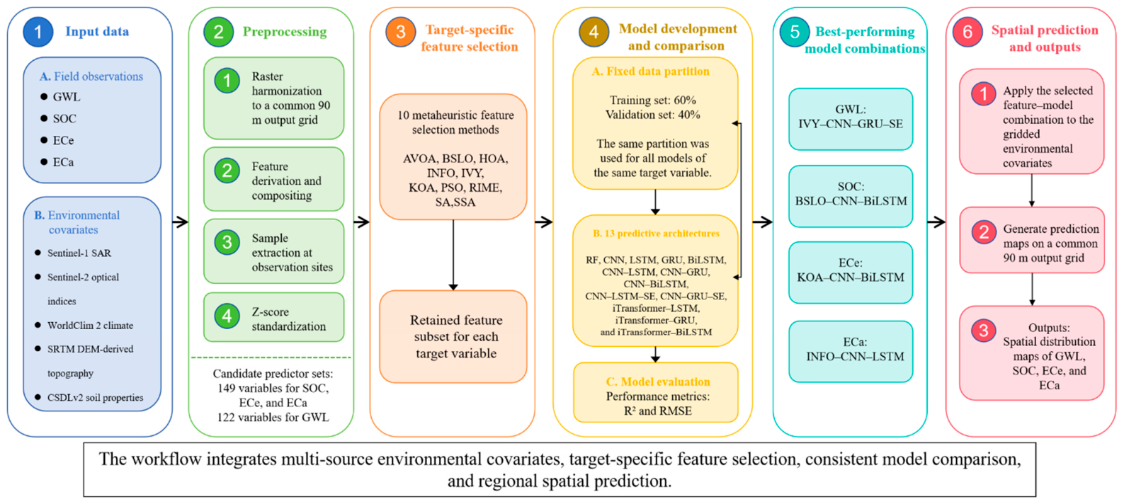
The overall methodological workflow is illustrated in Figure 2. It comprises the acquisition and preprocessing of field observations and multi-source environmental covariates, target-specific metaheuristic feature selection, consistent development and evaluation of predictive models, selection of the best-performing feature–model combination for each target variable, and final regional spatial prediction.

3.3. Metaheuristic Feature Selection Methods

Recent developments in metaheuristic optimization suggest that different algorithms adopt different strategies to balance global exploration and local exploitation, which may influence the predictor subsets identified during feature selection [69]. Therefore, before predictive modelling, metaheuristic feature selection was used to identify target-specific subsets of environmental covariates.
Ten methods were evaluated: the African Vultures Optimization Algorithm (AVOA), Blood-Sucking Leech Optimizer (BSLO), Hiking Optimization Algorithm (HOA), Weighted Mean of Vectors (INFO), Ivy Optimization Algorithm (IVY), Kepler Optimization Algorithm (KOA), Particle Swarm Optimization (PSO), RIME optimization algorithm (RIME), Simulated Annealing (SA), and Sparrow Search Algorithm (SSA). These methods represent different search paradigms, including swarm- and behaviour-inspired optimization, physics-based optimization, mathematical vector-update strategies, and probabilistic search. The original references and principal search mechanisms of the ten algorithms are summarized in Supplementary Table S4; therefore, their detailed operating mechanisms, search procedures, and update strategies are not described individually in the main text.
For each target variable, the ten methods were separately applied to the corresponding candidate predictor set. The initial predictor sets contained 149 covariates for ECe, SOC, and ECa and 122 covariates for GWL. Each feature selection method generated a target-specific retained subset, which was subsequently used as input to the same set of 13 predictive architectures. This common workflow enabled consistent comparison of the effects of the selected predictor subset, predictive architecture, and target variable on predictive performance. All metaheuristic feature-selection methods were implemented under a consistent computational setting. The population size was set to 2, and the maximum number of iterations was set to 50. For a target variable with p candidate covariates, each candidate solution was represented by a p-dimensional vector bounded between 0 and 1 and converted into a binary feature mask by rounding, where 1 indicated that the corresponding covariate was retained and 0 indicated exclusion. The initial candidate population was generated randomly within the search bounds. A fixed random seed of 1 was used consistently for all metaheuristic optimizers. Each candidate feature subset was evaluated using a random forest comprising 20 trees. Metaheuristic feature selection was conducted exclusively within the training set defined by the outer 6:4 train–validation split. During fitness evaluation, this training set was further randomly divided at a ratio of 6:4, with 60% used to fit the random forest and the remaining 40% used to calculate the sum of absolute prediction errors. This internal 6:4 partition was regenerated for each candidate feature-subset evaluation under the fixed random-seed setting. The outer validation set was not used at any stage of feature-subset optimization. The optimization objective was to minimize this error, and the subset yielding the lowest fitness value was retained for subsequent predictive modelling. Optimization was terminated after 50 iterations. Algorithm-specific control parameters followed their reference implementations. Each algorithm–target combination was executed once; therefore, variability across independent optimization runs was not evaluated in this study.

3.4. Machine Learning and Deep Learning Algorithms

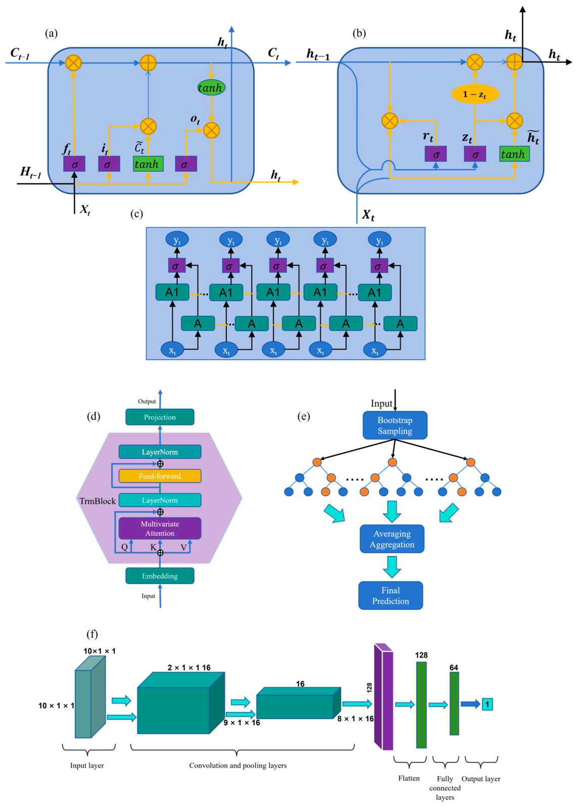
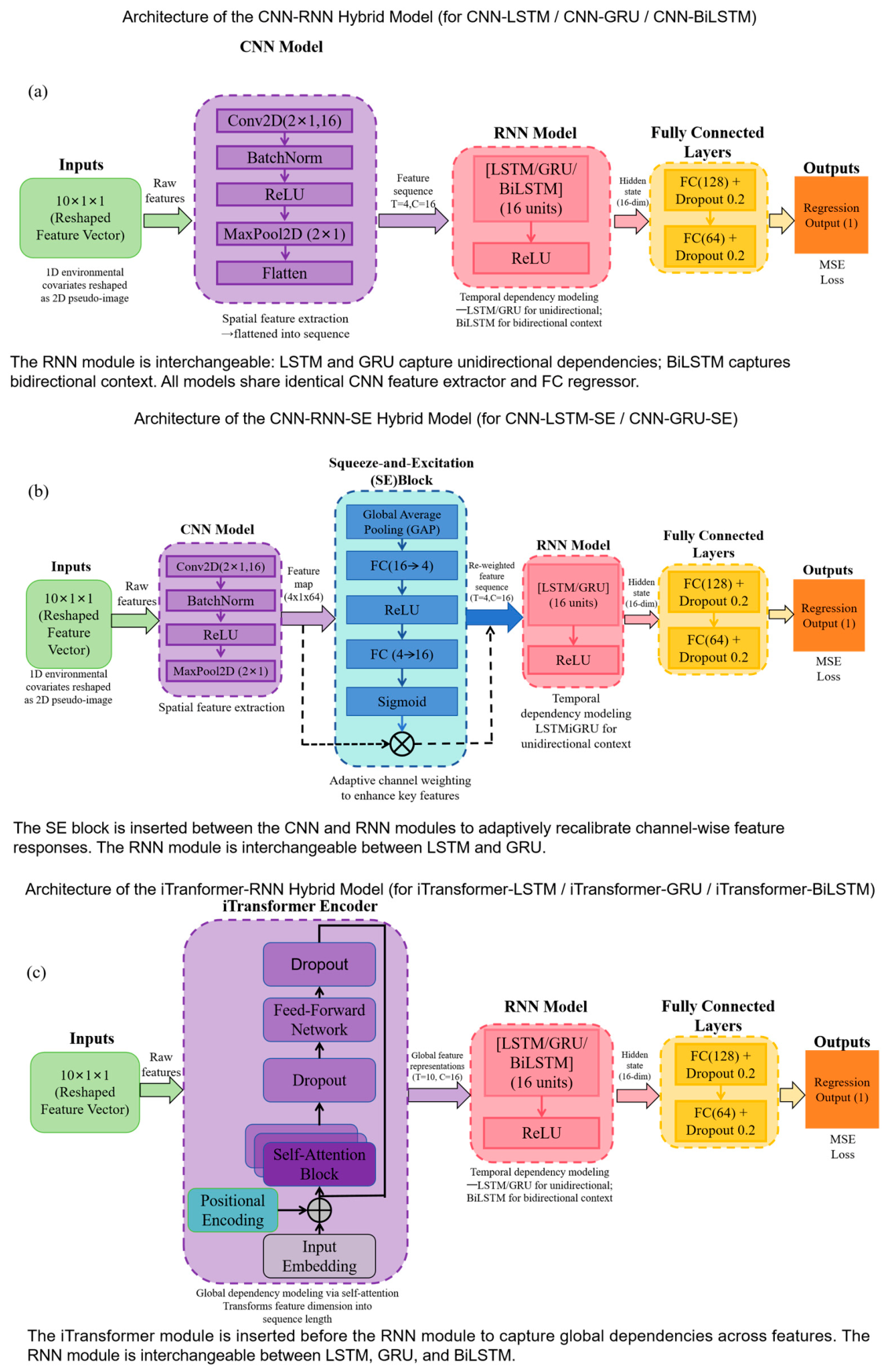
Predictive modelling of GWL, ECe, SOC, and ECa was performed using Python 3.12.5 on a 64-bit Windows 11 operating system. The machine learning and deep learning models were implemented using TensorFlow 2.21.0, Keras 3.14.1, and scikit-learn 1.8.0. All computations were conducted on a workstation equipped with a 13th Gen Intel Core i7-13650HX processor and 16 GB of RAM. The hyperparameter settings were primarily informed by commonly recommended configurations reported in the methodological literature for the corresponding architectures, including CNN [70], LSTM [71], GRU [72], BiLSTM [73], CNN–RNN hybrid architectures [74,75,76], SE-enhanced architectures [77,78], and iTransformer-based architectures [79]. These literature-informed settings were largely retained in the present study. Preliminary empirical testing was also conducted to assess the suitability of these configurations for the present datasets, but no systematic architecture-specific hyperparameter optimization was performed. Accordingly, the reported results represent the performance of the predefined configurations evaluated in this study and should not be interpreted as the maximum achievable performance of each architecture. For the recurrent and hybrid architectures, the selected environmental covariates at each sampling location were organized as a single-step input sequence with a sequence length of one. Therefore, the recurrent layers did not receive multitemporal observations and were evaluated as gated nonlinear representation components rather than as temporal forecasting models. The core hyperparameter configurations of the 13 predictive models are summarized in Table 2. The standalone base predictive model architectures are schematically illustrated in Figure 3.

3.4.1. Random Forest (RF)

RF is a machine learning algorithm employed for classification and regression that constructs an ensemble of multiple decision trees and aggregates their outputs to generate a final prediction [80]. In this study, the number of decision trees was set to 100, while other parameters remained at their default settings. RF is capable of modeling high-dimensional non-linear relationships, handling both categorical and continuous predictors, and exhibiting robustness against overfitting and noisy features [81]; thus, it is frequently utilized as a baseline comparison model.

3.4.2. Convolutional Neural Network (CNN)

The CNN represents one of the earliest deep learning architectures [52]. A typical CNN model comprises an input layer, several hidden layers (including convolutional, pooling, and fully connected layers), and an output layer [70]. The input data consisted of training points integrated with environmental attributes. Convolutional layers extract features through convolutional operations, followed by pooling layers to reduce data dimensionality and computational costs while mitigating overfitting. The pooled data were flattened into a one-dimensional vector and linked to a fully connected layer, with the final continuous predictions generated via the output layer. In this study, a 2D convolutional structure was adopted. The Adam optimizer was employed with a learning rate of 0.001, a batch size of 50, and 70 training epochs. Data were shuffled each epoch, with validation performed every 20 steps.

3.4.3. Long Short-Term Memory (LSTM)

LSTM is a specialized type of Recurrent Neural Network (RNN) designed to learn temporal features from time-series or sequential data [71]. A typical LSTM unit consists of a forget gate, an input gate, and an output gate, which collectively enable selective memory and the updating of temporal information. In this research, the LSTM model incorporated two hidden layers, each with 16 hidden units, a dropout rate of 0.2, and activation functions (Tanh and Sigmoid). The Adam optimizer was used with a learning rate of 0.001, a batch size of 50, and 70 epochs, utilizing Mean Squared Error (MSE) as the loss function.

3.4.4. Gated Recurrent Unit (GRU)

The GRU is a streamlined and improved version of the LSTM, offering comparable performance [72]. A GRU consists of two gates—the reset gate and the update gate—which cooperatively regulate the data flow within the memory cell to mitigate unnecessary informational redundancy. While maintaining the capacity to capture long-term dependencies, the GRU possesses a more concise architecture than the LSTM. During training, MSE was selected as the loss function, with parameters optimized via the Adam method.

3.4.5. Bidirectional Long Short-Term Memory (BiLSTM)

BiLSTM integrates forward and backward LSTM structures to simultaneously capture bidirectional contextual information from the input data [73]. In this study, the BiLSTM architecture contained two layers: the first layer output the complete sequence, and the second layer output the final time step. The bidirectional outputs were fused through concatenation. The hidden layer dimension was set to 16 with a dropout rate of 0.2 and Tanh/Sigmoid activation functions. The input sequence length was 1, and the Adam optimizer was utilized with a learning rate of 0.001.

3.4.6. CNN-RNN Hybrid Models

To further enhance spatial extraction and temporal modeling capabilities, hybrid architectures combining CNN with LSTM, GRU, and BiLSTM were designed. The CNN-LSTM architecture effectively fuses spatial feature extraction with temporal dependency learning, yielding superior predictions compared to standalone CNN or LSTM models [74]. The CNN-GRU architecture replaces LSTM with the lighter GRU to improve computational efficiency, reducing complexity and accelerating convergence while preserving sequence learning [75]. The CNN-BiLSTM architecture extends the framework by introducing bidirectional learning, enabling the network to synchronize past and future contextual information to enhance model stability and generalization in complex environments [76]. Local features were extracted by a CNN using a 2 × 1 convolutional kernel, 16 filters, and a stride of 1, followed by 2 × 1 max pooling. The resulting feature maps were fed into subsequent LSTM, GRU, or BiLSTM modules with hidden dimensions of 16. All models utilized the Adam optimizer (learning rate: 0.001, batch size: 68, 70 epochs) with MSE as the loss function.

3.4.7. CNN-RNN-SE Hybrid Models

The Squeeze-and-Excitation (SE) module was incorporated into the CNN–LSTM and CNN–GRU architectures to perform learned channel recalibration of intermediate feature maps [77]. The module applies channel-wise weights to modify the CNN feature representation and thereby increase its representational flexibility [78]. In this study, the CNN output 32 channels, which the SE module compressed to 16 before restoring weights via a Sigmoid activation. This module was followed by an LSTM or GRU (hidden dimension: 16, output mode: Last). Training parameters were consistent with those previously described.

3.4.8. iTransformer Hybrid Models

The iTransformer is a variant of the Transformer framework specifically designed to address issues encountered by autoregressive models when generating sequences in reverse order [79]. This model overcomes the limitations of traditional Transformers regarding large-scale backcast windows and conventional embedding strategies by combining self-attention mechanisms with positional encoding to extract global dependencies. This research integrated LSTM, GRU, and BiLSTM with the iTransformer to construct iTransformer-LSTM, iTransformer-GRU, and iTransformer-BiLSTM. The iTransformer encoder was configured with a maximum positional encoding length of 32, 2 attention modules, 1 attention head, a Key dimension of 2, a hidden dimension of 16, and a dropout rate of 0.2. The extracted features were then processed by LSTM, GRU, or BiLSTM modules with a hidden dimension of 16 and a sequence length of one to provide gated nonlinear transformations of the learned representation. All other training parameters were identical to those used for the corresponding recurrent models. The schematic architectures of the hybrid deep learning models evaluated in this study are illustrated in Figure 4.

3.5. Model Interpretation Using SHAP

To improve the interpretability of the deep learning models, SHapley Additive exPlanations (SHAP) analysis was conducted for the best-performing model associated with each target variable [82]. SHAP values quantify the contribution of individual environmental covariates to each prediction relative to the expected model output, thereby enabling the importance and direction of feature contributions to be examined.
Global feature importance was quantified using the mean absolute SHAP value. SHAP summary plots were used to jointly display the relative importance of the environmental covariates, the magnitude of their feature values, and the direction of their contributions to the model output. The 20 most influential environmental covariates were displayed for each prediction task.

3.6. Model Performance Evaluation Metrics

For each target variable, the available observations were randomly divided into a training set and a holdout validation/model-selection set at a ratio of 6:4 using a fixed random seed of 1. The training set, comprising 60% of the observations, was used for model fitting, whereas the remaining 40% served as a common holdout set for evaluating all feature-selection–architecture combinations and identifying the best-performing combination for each target variable. No independent test set was established in this study. This outer holdout set was kept separate from the internal RF-based fitness evaluation used during metaheuristic feature selection and was not accessed during feature-subset optimization. The same data partition was applied to all feature-selection methods and predictive architectures for the corresponding target variable to ensure a consistent basis for comparison. The predefined hyperparameters of each predictive architecture were also kept unchanged throughout the comparisons. Before model training, both the environmental covariates and target values were standardized using Z-score transformation. The means and standard deviations calculated from the training set were used to standardize both the training and validation data.
In this study, model performance was evaluated consistently across all feature-selection–architecture combinations using the coefficient of determination (R2) and root mean square error (RMSE). R2 was used to quantify the proportion of variance in the observations explained by the predictions, whereas RMSE quantified the magnitude of prediction errors in the original unit of each target variable, with greater weight given to larger errors. These two metrics were selected to provide a consistent basis for comparing the large number of model combinations evaluated across the four prediction tasks. Higher R2 and lower RMSE values therefore indicate better performance under these evaluation criteria.
R 2 = 1     i = 1 n y i     y i ^ 2 i = 1 n y i     y ¯ 2
RMSE = 1 n i = 1 n y i     y i ^ 2
where y i and y i ^ denote the observed and predicted values, respectively, y ¯ is the mean of the observed values, and n is the number of observations.
To compare each learning architecture with the corresponding RF baseline under the same feature selection method, both the absolute difference in R2 and the relative change in R2 were calculated as follows:
Δ R 2 = R model 2 R RF 2
I R 2 % = R model 2 R RF 2 R RF 2 × 100

4. Results

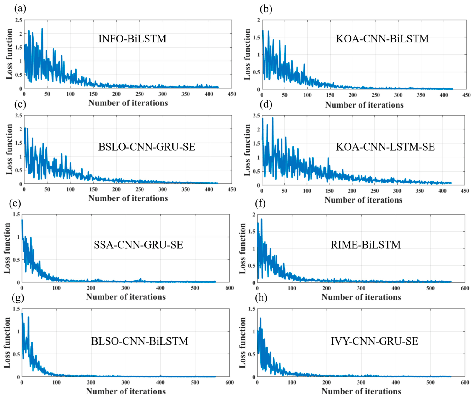
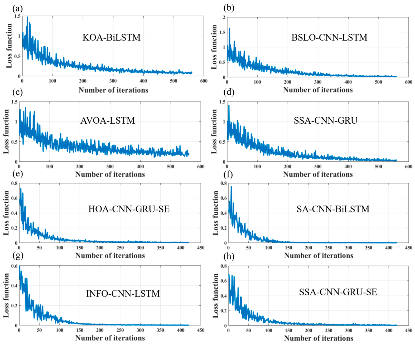
Figure 5 and Figure 6 present the training-loss trajectories of representative deep learning models for the four prediction tasks, showing a rapid decline during the initial iterations followed by gradual convergence.

4.1. Descriptive Statistics of Soil and Groundwater Properties

Table 3 presents the descriptive statistical characteristics of the various soil and groundwater properties within the study area. In Northern Xinjiang, the SOC content ranged from 0.49 g/kg to 68.76 g/kg, with a mean value of 8.15 g/kg. The ECe values varied between 37.4 μS/cm and 38,975 μS/cm, averaging 1920.87 μS/cm. In the Tarim River Basin of Southern Xinjiang, the GWL depth ranged from 0.79 m to 150.24 m, with an average depth of 12.25 m. Additionally, the ECa values ranged from 1.39 mS/m to 1763.94 mS/m, with a mean value of 338.13 mS/m.

4.2. Feature Selection Results Based on Diverse Optimization Algorithms

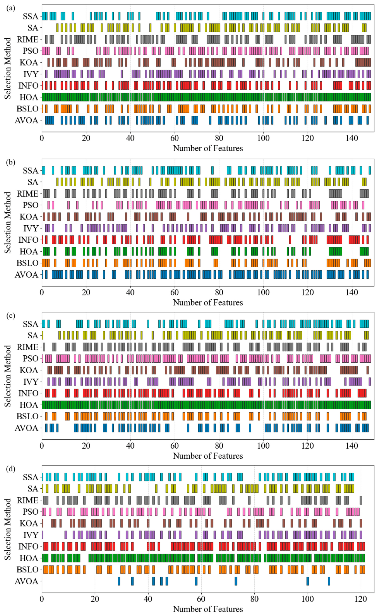
In this study, ten distinct feature selection methods (AVOA, BSLO, HOA, INFO, IVY, KOA, PSO, RIME, SA, and SSA) were individually employed to select environmental covariates across four datasets. Figure 7 illustrates the number of covariates identified by these methods for GWL, ECe, SOC, and ECa across the study regions. As shown in Figure 7b, the number of environmental covariates selected for SOC in Northern Xinjiang was 93 (AVOA), 69 (BSLO), 65 (HOA), 77 (INFO), 72 (IVY), 69 (KOA), 69 (PSO), 65 (RIME), 75 (SA), and 75 (SSA). Figure 7a reveals that for ECe, the number of selected covariates was 67 (AVOA), 73 (BSLO), 149 (HOA), 77 (INFO), 78 (IVY), 73 (KOA), 87 (PSO), 82 (RIME), 75 (SA), and 78 (SSA). Furthermore, Figure 7c,d present the results for ECa and GWL in the Tarim River Basin of Southern Xinjiang, respectively. Specifically, for ECa, the count of selected covariates was 71 (AVOA), 76 (BSLO), 149 (HOA), 85 (INFO), 77 (IVY), 82 (KOA), 107 (PSO), 80 (RIME), 76 (SA), and 76 (SSA). In contrast, the counts for GWL were 9 (AVOA), 64 (BSLO), 112 (HOA), 84 (INFO), 57 (IVY), 47 (KOA), 64 (PSO), 56 (RIME), 62 (SA), and 59 (SSA).
As evidenced by Figure 7, the HOA method consistently selected the highest number of environmental covariates for GWL, ECe, and ECa, reaching 112, 149, and 149, respectively; however, for SOC, the count for HOA was significantly lower at 65. Conversely, AVOA yielded the most parsimonious feature subsets for GWL, ECe, and ECa, with only 9, 67, and 71 covariates selected, while selecting 93 for SOC. While most feature selection methods maintained a comprehensive selection of covariates, HOA notably included the entire set of available environmental covariates for both the ECe and ECa datasets. Particularly, an extreme case occurred in the GWL dataset, where AVOA selected only 9 out of 122 possible environmental covariates.
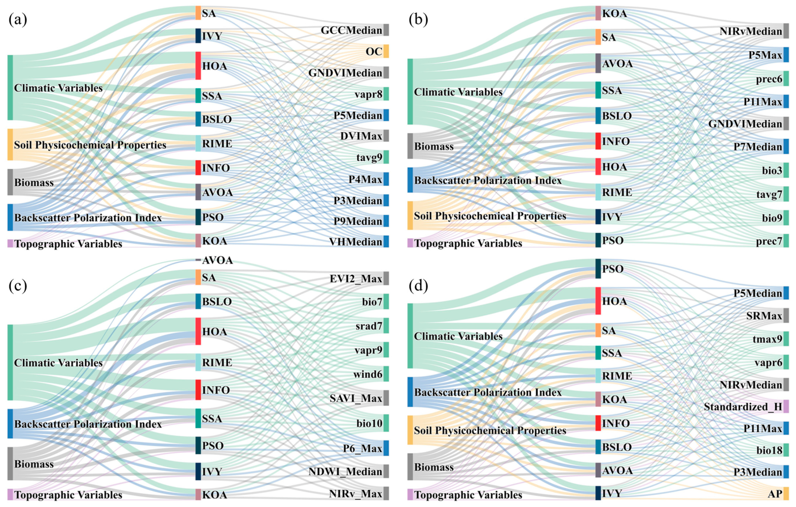
To further investigate the primary composition of the variables identified by each feature selection method, Figure 8 visually illustrates the key environmental covariates selected across the four datasets. As depicted in the figure, although the number of essential covariates retained varies among the different methods, climatic variables consistently maintain a dominant position across all feature selection techniques. The right panel of Figure 8 further elucidates the specific variables prioritized by each method. For the GWL dataset (Figure 8c), the significance of climatic variables is particularly pronounced; numerous feature selection algorithms consistently identified variables closely related to temperature and water vapor pressure, such as wind6, vapr9, and bio10. Conversely, for the SOC and salinity indicators (ECe and ECa) (Figure 8a,b,d), in addition to climatic factors, remote sensing and radar indices reflecting surface vegetation cover—such as GNDVIMedian, EVI2_Max, P11Median, and NIRvMedian—also emerged as highly frequently selected variables across the various methods.

4.3. Impact of Different Feature Selection Methods on Model Performance

Table 4 summarizes the mean R2, mean RMSE, standard deviations, and corresponding coefficients of variation calculated across the evaluated predictive architectures for each feature-selection method and prediction target. These statistics are descriptive summaries across predictive architectures and do not represent repeated independent optimization runs or inferential estimates of algorithmic stability. The results showed clear target-dependent differences in both predictive performance and cross-architecture variability, and no method consistently ranked first for all evaluation metrics.
For GWL prediction, INFO achieved the highest mean R2 and the lowest mean RMSE, indicating strong average predictive performance. However, KOA produced lower coefficients of variation for both R2 and RMSE, indicating lower performance variability across the evaluated predictive architectures. Thus, the method with the highest average predictive performance was not necessarily the method with the most consistent performance across architectures.
For ECe, IVY and KOA achieved the highest mean R2, while KOA yielded the lowest mean RMSE. Their average performance was relatively similar, although IVY showed slightly lower variability in R2. In comparison, PSO showed comparatively weaker average performance. These results indicate that feature selection influenced not only average model performance but also the sensitivity of subsequent models to the selected predictor subset.
For ECa, INFO and KOA obtained the highest mean R2, whereas IVY achieved the lowest mean RMSE. Nevertheless, the coefficients of variation remained comparatively high for several methods, indicating that ECa prediction was more sensitive to the interaction between feature selection and model architecture than GWL prediction. For SOC, AVOA and BSLO achieved the highest mean R2, with AVOA also producing the lowest mean RMSE. However, HOA exhibited lower variation in R2 than AVOA and BSLO, again showing that the method yielding the highest average performance did not always provide the most consistent results across architectures.
Overall, the differences among R2, RMSE, and their coefficients of variation demonstrate that feature selection methods should not be evaluated using a single metric. Methods that achieved a high mean R2 did not necessarily produce the lowest prediction error or the lowest variability across predictive architectures. The relative effectiveness of each feature selection method therefore depended on the target variable and its compatibility with the subsequent predictive architecture.

4.4. Performance Comparison of Standalone Machine Learning Algorithms

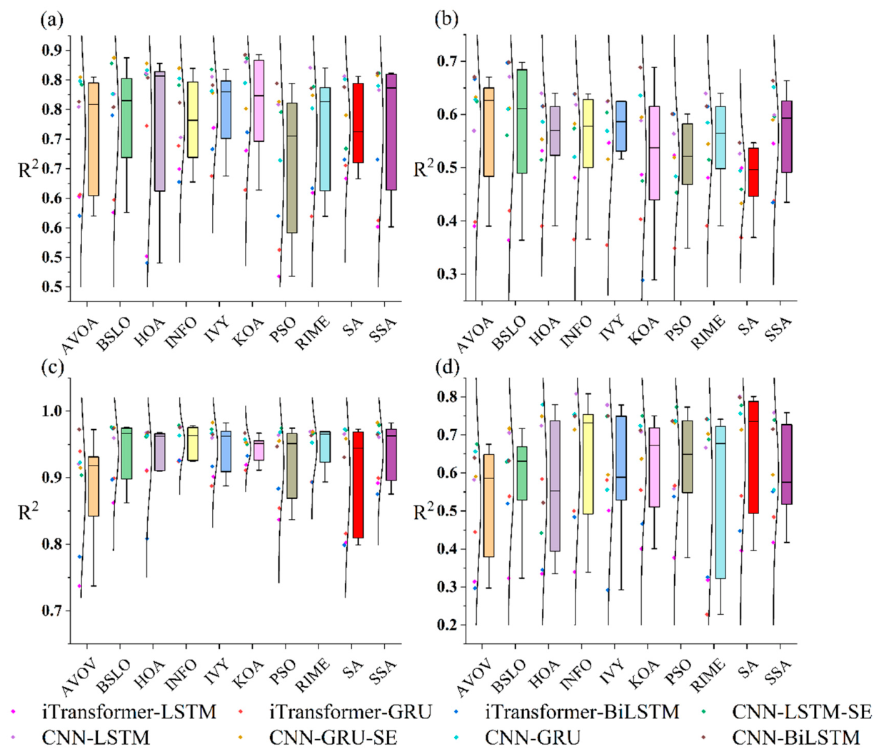
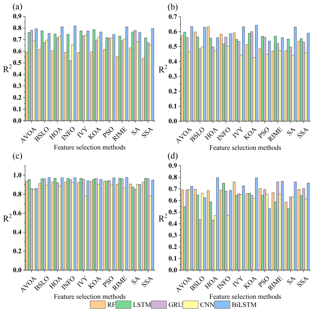
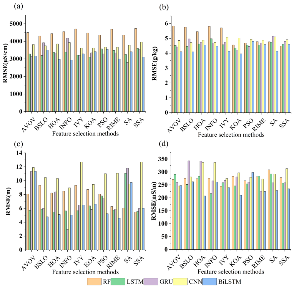
To systematically evaluate the performance of different standalone machine learning algorithms in predicting GWL, ECe, SOC, and ECa, this study constructed five categories of models—RF, LSTM, GRU, CNN, and BiLSTM—integrated with various feature selection methods. Their predictive capabilities were specifically assessed utilizing R2 and RMSE. Figure 9 and Figure 10 present the R2 and RMSE of these models across the different datasets, respectively.
As illustrated in Figure 9, all evaluated models exhibited varying degrees of predictive capability across the four tasks, with BiLSTM achieving the optimal R2 values in the vast majority of cases. Specifically, in the prediction results for GWL, ECe, SOC, and ECa (Figure 9c, Figure 9a, Figure 9b, and Figure 9d, respectively), the combinations of BiLSTM and various feature selection methods secured the highest frequency of optimal R2 occurrences, achieving them 5, 6, 5, and 6 times, respectively. Furthermore, BiLSTM consistently attained the highest predictive R2 across all four tasks, reaching 0.9777 for GWL, 0.8169 for ECe, 0.6436 for SOC, and 0.7971 for ECa. Concurrently, the BiLSTM combinations demonstrated outstanding performance in predictive error control. In the ECe predictions, its RMSE generally remained below 3541.43 μS/cm; for SOC, the RMSE was typically under 4.60 g/kg; in GWL predictions, the RMSE was lower than 11.34 m; and for ECa, it was generally below 298.13 mS/m. In addition, the LSTM and GRU combinations exhibited prominent performance in GWL prediction. Specifically, the RIME-LSTM model achieved an R2 and RMSE of 0.9673 and 5.73 m, respectively. Similarly, the KOA-GRU model recorded an R2 of 0.9646 and an RMSE of 5.84 m. Based on the GWL prediction results, the five standalone architectures generally achieved strong predictive performance; the lowest R2 was 0.7804 (produced by both SSA–CNN and IVY–CNN), while the highest R2 was 0.9777 (produced by RIME–BiLSTM). Moreover, the R2 values of the individual models for GWL showed comparatively lower variation than those for the other datasets, with the majority exceeding 0.90.

4.5. Performance Comparison of Different Algorithm Combinations

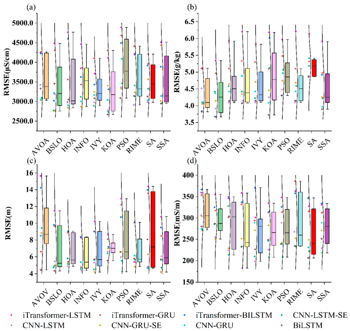
To enhance the predictive efficacy for GWL, ECe, SOC, and ECa, this study integrated various model algorithms and introduced attention mechanisms, subsequently evaluating the R2 and RMSE of these hybrid architectures. Figure 11 and Figure 12 illustrate the performance comparisons of integrations between the 10 feature selection methods and 8 hybrid algorithms for predicting GWL, ECe, ECa, and SOC. Overall, the CNN–RNN hybrid architectures generally achieved strong predictive performance across the evaluated prediction tasks.
In the ECe prediction results (Figure 11a and Figure 12a), the KOA-CNN-BiLSTM model achieved the highest R2 (0.8429), alongside the lowest RMSE of 2666.87 μS/cm, among all evaluated combinations. For the SOC prediction results (Figure 11b and Figure 12b), BSLO-CNN-BiLSTM achieved the optimal R2 (0.6981), with a corresponding RMSE of 3.67 g/kg. In the context of GWL prediction, IVY-CNN-GRU-SE yielded the best predictive performance, recording an R2 and RMSE of 0.9826 and 4.20 m, respectively; conversely, AVOA-iTransformer-LSTM performed the poorest, with an R2 of 0.7373 and an RMSE of 15.65 m. Regarding ECa prediction, INFO-CNN-LSTM performed outstandingly, achieving an R2 and RMSE of 0.8085 and 182.69 mS/m, respectively, whereas RIME-iTransformer-GRU exhibited the poorest performance (R2: 0.2275, RMSE: 386.19 mS/m).
Notably, compared to standalone algorithms, certain hybrid architectures underperformed in terms of predictive accuracy. For instance, the R2 of the hybrid INFO-iTransformer-BiLSTM decreased by 0.1893 compared to the standalone INFO-BiLSTM in the ECe dataset. In the SOC dataset, the R2 of KOA-iTransformer-BiLSTM dropped by 0.3547 relative to KOA-BiLSTM. For the ECa dataset, the R2 of HOA-iTransformer-BiLSTM decreased by 0.0150 compared to HOA-BiLSTM. Furthermore, in the GWL dataset, the R2 of AVOA-CNN-LSTM-SE decreased by 0.0505 and its RMSE increased by 3.70 m compared to the standalone AVOA-LSTM. Similarly, the R2 of KOA-CNN-GRU-SE dropped by 0.0120 and its RMSE rose by 1.14 m compared to KOA-GRU.

4.6. Comparative Analysis of Model Performance Enhancements

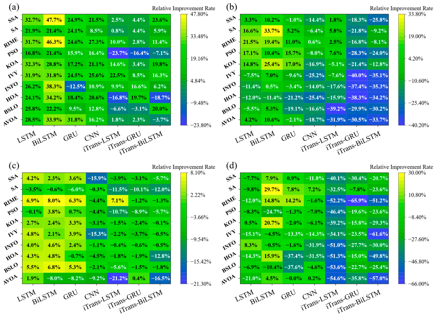
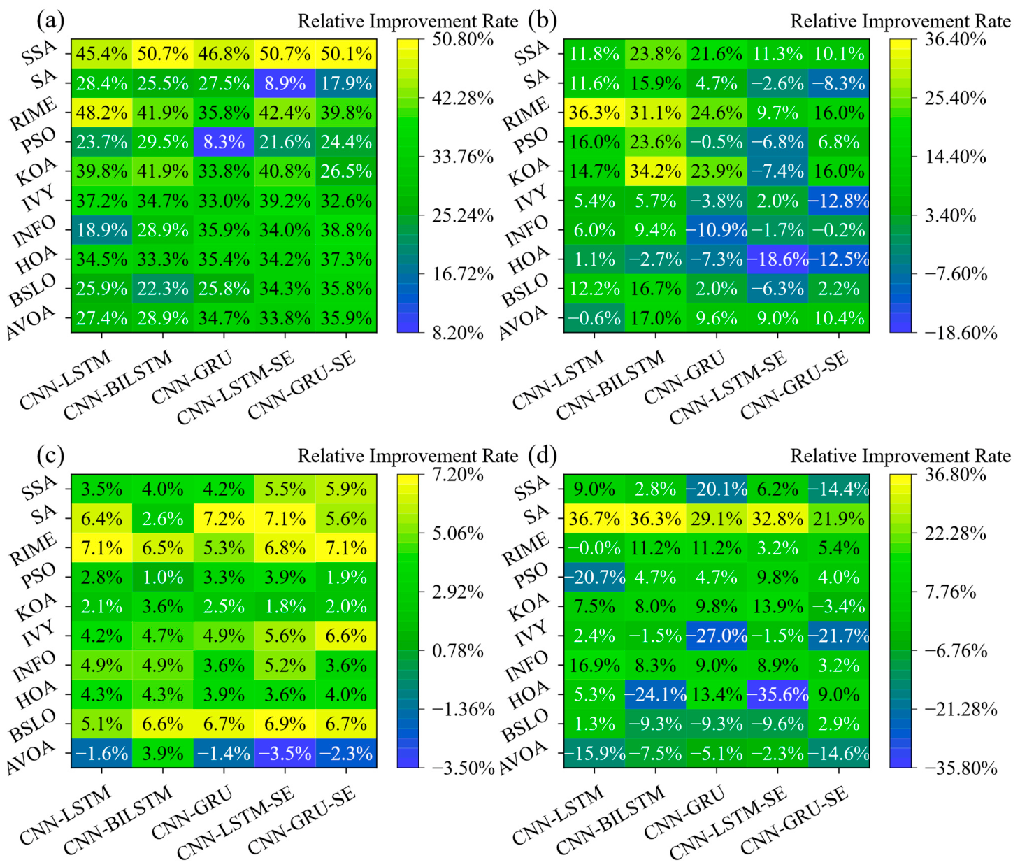
To quantify differences between the evaluated learning architectures and conventional machine learning, RF was used as the baseline under each feature selection method. Both the absolute difference in R2  Δ R 2 and the relative change in R2  I R 2 were calculated. Figure 13 and Figure 14 present the relative R2 changes for the standalone, iTransformer-based, and CNN–RNN architectures, while representative absolute R2 differences are reported in the accompanying text.
In the ECe dataset (Figure 13a and Figure 14a), both standalone and hybrid models exhibited substantial positive enhancements. As shown in Figure 13a, among the standalone and iTransformer-based models, the combinations of BiLSTM with various feature selection methods generally showed substantial improvements, with the enhancement rates of the RIME-BiLSTM and SSA-BiLSTM models reaching 42.3% and 47.7%, respectively. Conversely, the iTransformer-based models showed smaller margins of improvement, with some combinations yielding negative enhancement rates, such as PSO-iTransformer-LSTM and PSO-iTransformer-GRU at −23.7% and −16.4%, respectively. As depicted in Figure 14a, the overall performance of hybrid models incorporating CNN and attention mechanisms improved markedly, with the vast majority of areas displaying bright yellow; among these, SSA-CNN-LSTM-SE and SSA-CNN-BiLSTM recorded the highest relative enhancement rates, both exceeding 50%.
In the SOC dataset, the performance of different models exhibited pronounced divergence. As shown in Figure 13b, only a subset of the standalone models achieved positive enhancements, with SA-BiLSTM securing the highest improvement of 33.7%. However, under feature selection methods such as IVY and INFO, multiple models experienced notable performance degradation. In contrast, the hybrid models in Figure 14b showed fewer negative performance changes, with a noticeable reduction in negative-value regions. Notably, the hybrid models under the RIME feature selection method stood out, with RIME-CNN-LSTM achieving a 36.3% performance gain.
For the GWL dataset, the overall relative enhancement margins were minor, with a highly concentrated numerical distribution. As illustrated in Figure 13c, the relative enhancement rates of the models generally ranged between −10% and 8%. The best-performing combination was RIME-BiLSTM, which improved by 8.0% relative to RF, whereas the corresponding AVOA-iTransformer-BiLSTM experienced a decline of −16.5%. Regarding the hybrid models (Figure 14c), their enhancement margins also remained at a lower level, though they showed a higher proportion of positive performance improvements. SA-CNN-GRU and SA-CNN-LSTM-SE achieved enhancements of 7.2% and 7.1%, respectively, with the majority of combinations showing improvements concentrated in the 1% to 6% range.
The two sets of charts for the ECa dataset revealed a stark contrast. As shown in Figure 13d, the standalone and iTransformer-based models displayed extensive negative values—with RIME-iTransformer-GRU even registering a −65.9% drop—while only a few models, such as SA-BiLSTM, yielded positive enhancements (29.7%). However, this situation was partially ameliorated among the hybrid models (Figure 14d), particularly under the SA feature selection method, where CNN-LSTM and CNN-BiLSTM achieved positive enhancements of 36.7% and 36.3%, respectively. Although negative values persisted under certain feature selection methods (e.g., RIME, HOA), the overall performance exhibited a noticeable recovery compared to the standalone models.

4.7. SHAP-Based Interpretation of the Best-Performing Models

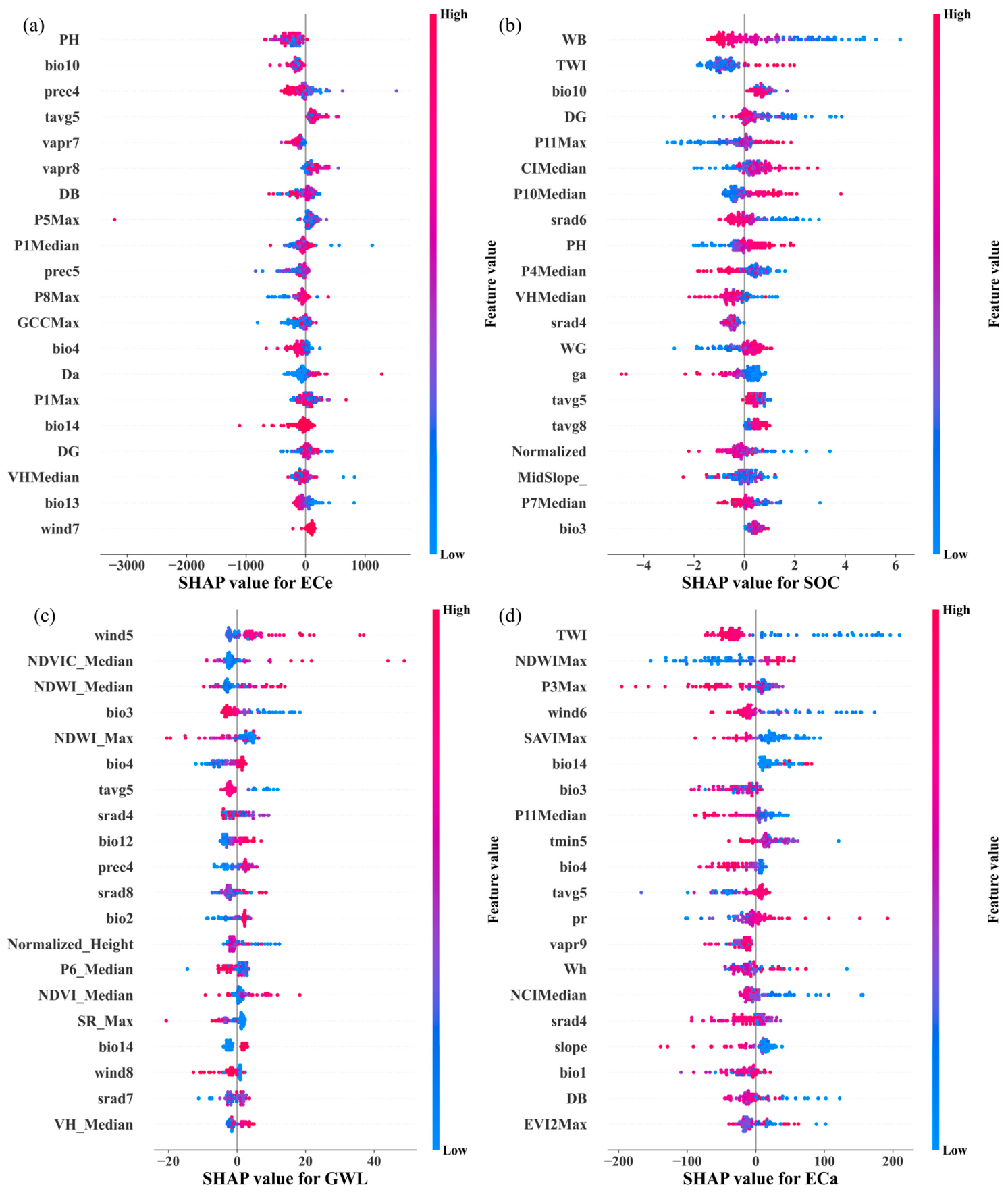
The SHAP beeswarm plots revealed clear differences in the environmental covariates contributing to the predictions of ECe, SOC, GWL, and ECa (Figure 15). Both the importance rankings and contribution directions varied among the four targets, indicating that the best-performing models relied on different combinations of climatic, remotely sensed, topographic, and soil-related information.
For ECe prediction (Figure 15a), PH, bio10, prec4, tavg5, and vapr7 were the five highest-ranked covariates. Higher PH, bio10, prec4, and vapr7 values were generally associated with negative SHAP values, whereas higher tavg5 values tended to increase the model output. Several lower-ranked covariates showed wider or bidirectional SHAP distributions, indicating that their contributions varied among samples.
For SOC prediction (Figure 15b), WB made the largest overall contribution, followed by TWI, bio10, DG, and P11Max. Higher WB and DG values were mainly associated with negative contributions, whereas higher TWI, bio10, and P11Max values generally increased the predicted SOC values. The broad SHAP distributions of WB, TWI, and DG further suggest that their effects differed across environmental settings.
For GWL prediction (Figure 15c), wind5 was the most influential covariate, followed by NDVIC_Median, NDWI_Median, bio3, and NDWI_Max. Higher wind5, NDVIC_Median, and NDWI_Median values generally produced positive contributions, whereas higher bio3 and NDWI_Max values were predominantly associated with negative SHAP values. Climatic variables such as tavg5, srad4, bio12, and prec4 also ranked prominently, showing that the model relied strongly on climatic, vegetation, and surface-moisture information.
For ECa prediction (Figure 15d), TWI, NDWIMax, P3Max, wind6, and SAVIMax were the five most influential covariates. Higher TWI, P3Max, wind6, and SAVIMax values generally reduced the model output, whereas higher NDWIMax values were mainly associated with positive contributions. The importance of these terrain-, vegetation-, moisture-, and climate-related covariates indicates that the ECa model integrated several types of environmental information.
Overall, no single environmental covariate dominated all four prediction tasks. The target-specific rankings and contribution directions, together with the broad or bidirectional distributions observed for several variables, indicate that the models captured nonlinear and context-dependent relationships among environmental covariates and the predicted properties.

4.8. Fitting Relationship Between Predicted and Observed Values

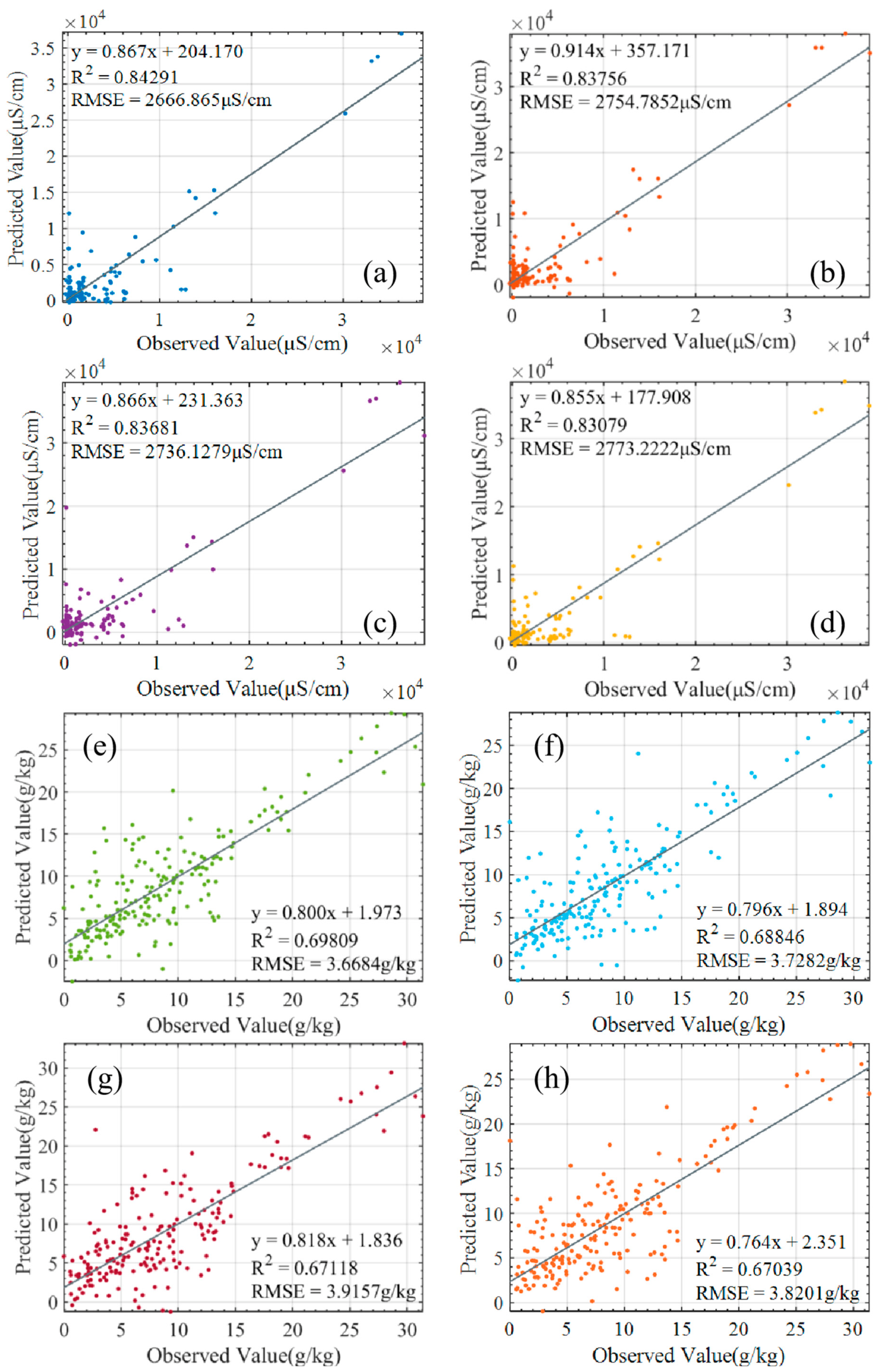
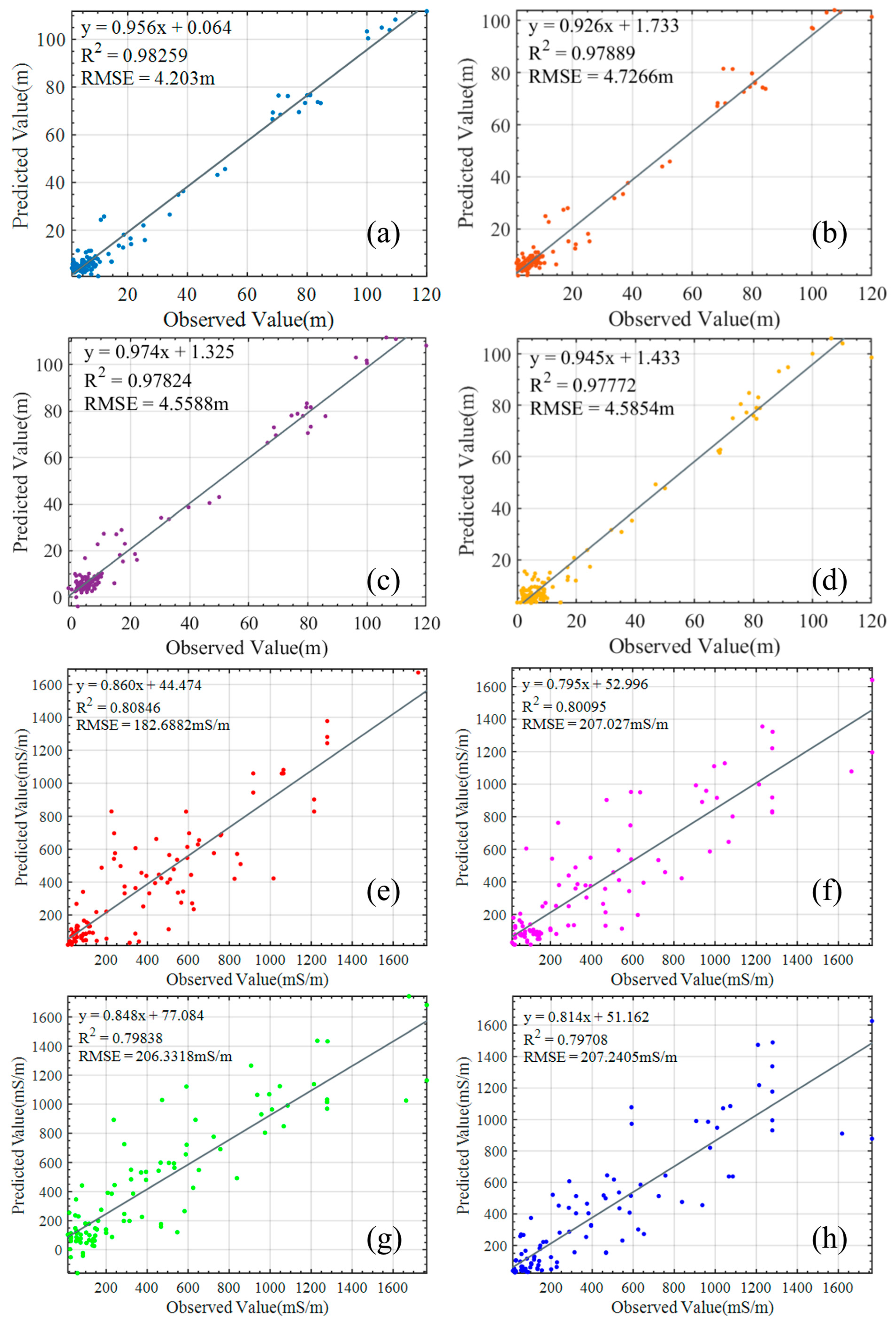
To visually evaluate the fit of the best-performing hybrid models across the four prediction tasks, we selected the top four model combinations for ECe, SOC, GWL, and ECa and plotted their predicted values against the corresponding observations (Figure 16 and Figure 17). Overall, the predicted and observed values showed varying degrees of agreement across the four target variables, with the closest correspondence observed for the best-performing models.
Specifically, for the GWL dataset (Figure 17a–d), the scatter points exhibited an outstanding degree of fit within the observed range of 0–120 m. The data tightly clustered around the fitting lines, indicating a low overall degree of dispersion. Based on the fitting equations, the regression slopes for these four models ranged from 0.926 to 0.974, with intercepts distributed between 0.064 and 1.733; these near-unity slopes and minimal intercepts underscore highly accurate predictions. In contrast, within the ECe dataset (Figure 16a–d), the vast majority of scatter points were densely concentrated in the low-value interval of 0–5000 μS/cm, whereas the distribution became noticeably sparser in the high-value region above 20,000 μS/cm. Under this skewed distribution pattern, the linear fitting slopes of the models ranged from 0.855 to 0.914, with intercepts falling between 177.908 and 357.171. The sparse representation of high ECe values may have increased prediction uncertainty in the extreme-value range, as model performance across wide and skewed value distributions can depend on both data preprocessing and model architecture [83]. Future studies could evaluate ensemble strategies or models specifically designed to improve predictions for extreme ECe values.
Regarding the ECa dataset (Figure 17e–h), the observed values generally spanned from 0 to 1700 mS/m, with scatter points heavily aggregated in the low-value zone below 200 mS/m. As the observed values increased, the point density in the high-value region gradually decreased, and the degree of dispersion exhibited an expanding trend—a characteristic indicative of increased variance at higher values. The model slopes for this dataset fell between 0.795 and 0.860, and the intercepts ranged from 44.474 to 77.084. Finally, for the SOC dataset (Figure 16e–h), the scatter points were distributed relatively uniformly across the 0–30 g/kg interval, lacking the extreme clustering phenomena observed in the ECe and ECa datasets. However, the SOC dataset displayed the highest overall dispersion among the four groups. The points were more sparsely distributed along the fitting lines, corresponding to regression slopes between 0.764 and 0.818, and intercepts ranging from 1.836 to 2.351.
Taken together, the results revealed three principal patterns. First, the effectiveness of feature selection was strongly target-dependent, and no single method consistently achieved the best combination of model fit, prediction error, and low cross-architecture variability across GWL, ECe, SOC, and ECa. Second, CNN–RNN hybrid architectures generally achieved higher predictive performance than standalone and iTransformer-based models, although the magnitude of improvement varied among the four prediction tasks. The best-performing combinations achieved R2 values of 0.9826, 0.8429, 0.6981, and 0.8085 for GWL, ECe, SOC, and ECa, respectively. Third, the relatively small performance gains observed for GWL and the greater variability found for SOC and ECa indicate that the benefits of increasing model complexity depended on both the strength of the target–covariate relationships and the compatibility between the selected feature subset and the predictive architecture. These findings demonstrate that the observed performance differences were structured rather than uniform, with feature selection, model architecture, and target characteristics jointly determining the predictive benefit of increasing model complexity.
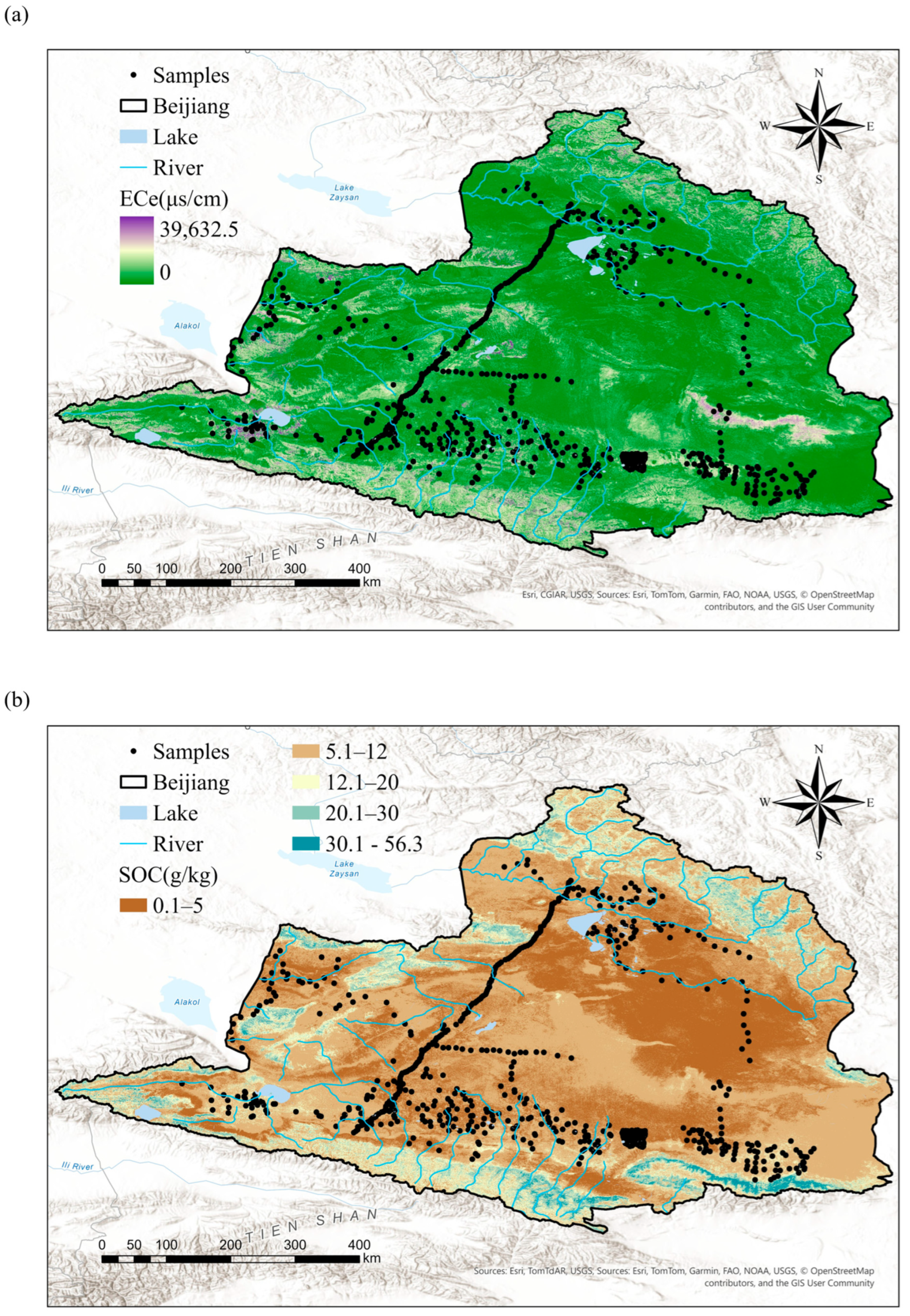
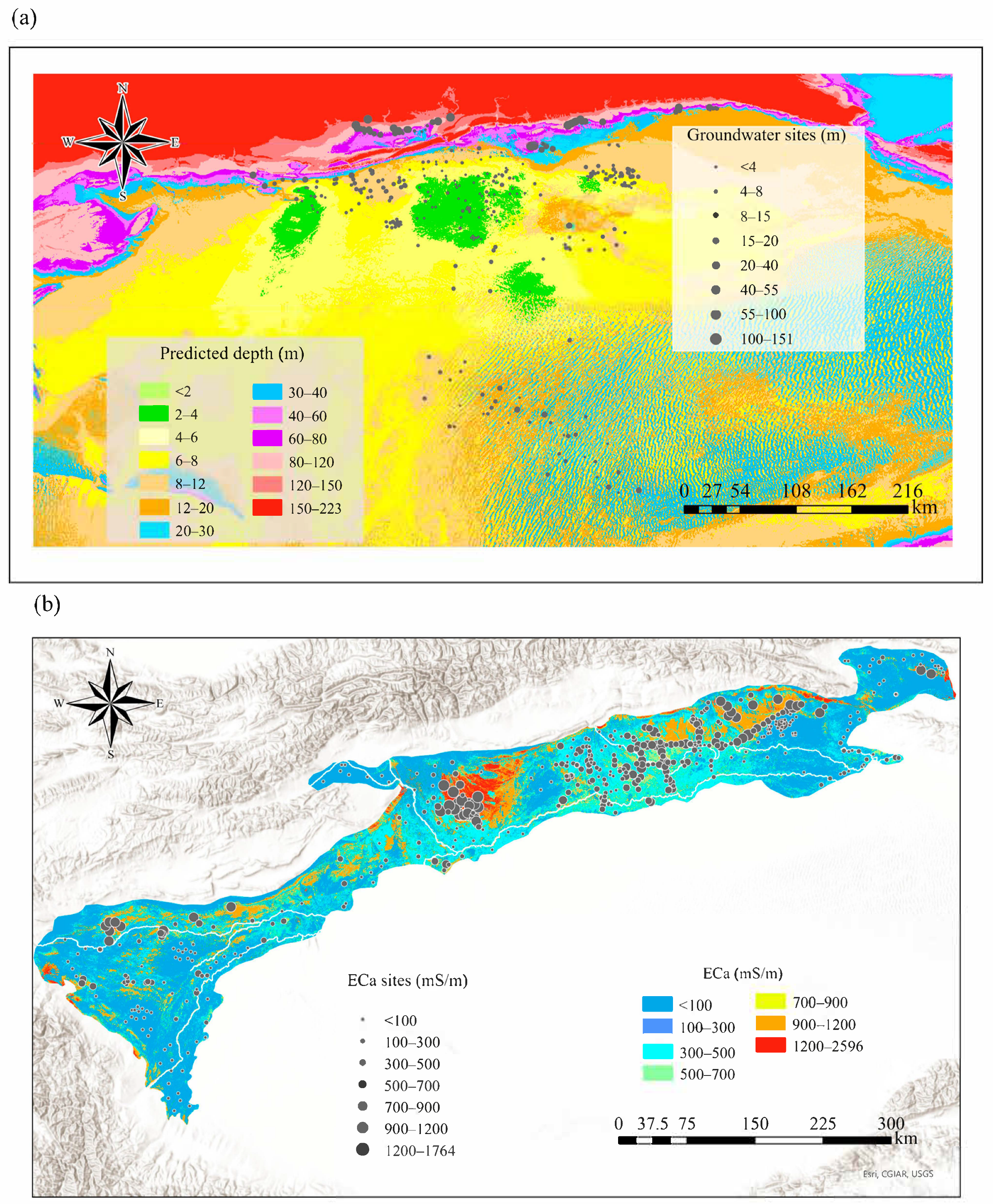
On the basis of these comparative and diagnostic results, the best-performing feature-selection–architecture combination for each target was subsequently applied to regional spatial prediction. The resulting maps show the predicted distributions of ECe and SOC in Northern Xinjiang and of GWL and ECa in Southern Xinjiang, as presented in Figure 18 and Figure 19, respectively.

5. Discussion

5.1. Performance Differences Among Algorithms and the Synergistic Enhancement of Hybrid Modeling

Through a systematic evaluation of four agro-environmental datasets, this study compared the predictive performance of different model architectures and examined the conditions under which hybrid architectures provided improvements over standalone models. The observed performance differences occurred both between model categories and among individual model configurations. The best-performing combinations in this study yielded R2 values comparable to or numerically higher than those reported for several models in previous studies of similar arid environments. Specifically, in GWL prediction, the IVY–CNN–GRU–SE model achieved an R2 of 0.9826, compared with 0.94 for the GRU model reported by Gharehbaghi et al. [84] and 0.90 for the CNN–GRU–Attention model reported by Wei et al. [85]. Regarding SOC, the proposed BSLO–CNN–BiLSTM achieved an R2 of 0.6981, compared with 0.675 for the Gradient Boosting model reported by Chen et al. [86] and 0.65 for the traditional Deep Neural Network (DNN) reported by Emadi et al. [87]. For soil salinity indicators, the proposed KOA–CNN–BiLSTM reached an R2 of 0.8429 in ECe prediction, compared with 0.77 for the KNN model reported by Chaaou et al. [39]. Additionally, the INFO–CNN–LSTM model optimized for ECa achieved an R2 of 0.8085, compared with the R2 of 0.74 obtained by Wang et al. [88] through multi-algorithm comparisons in the Kuqa Oasis, Xinjiang.
Contrasting findings have also been reported in previous studies. Müller et al. [89] found that a relatively simple multilayer perceptron outperformed LSTM and CNN models for groundwater prediction in terms of both predictive accuracy and computational efficiency, despite systematic hyperparameter optimization. For soil salt dynamics, Lei et al. [90] showed that model rankings changed with the prediction scenario and predictor set: distributed random forest performed best when only limited in-field inputs were available, gradient boosting improved as additional variables were introduced, and deep learning became more competitive in cross-field prediction, particularly for deeper soil layers and later crop growth stages. These findings differ from the generally stronger performance of several CNN–RNN hybrids observed in the present study. Such disagreement may be related to differences in environmental conditions, sample size and spatial density, predictor composition, input representation, and validation strategy. In particular, the present study used static point-level environmental covariates with a sequence length of one, whereas the contrasting studies incorporated different forms of temporal information or field-transfer scenarios. Therefore, model superiority should be regarded as task- and data-dependent rather than as an inherent consequence of architectural complexity.
Among the standalone models, LSTM and BiLSTM generally achieved higher R2 values than RF and CNN under several feature selection methods. However, because the environmental covariates were static and the input sequence length was one, this performance cannot be attributed to the learning of long-term temporal dependencies. A more plausible interpretation is that the gated cells provided additional multiplicative nonlinear transformations and adaptive information modulation when processing the selected covariates. LSTM-inspired gates have also been used in non-recurrent deep networks to regulate information flow across layers [91], while gated architectures can suppress unnecessary processing components when integrating static covariates [92]. More broadly, research on deep tabular learning has shown that adaptively transforming and weighting salient input variables can improve the representation of heterogeneous covariates [93]. Therefore, the performance of LSTM and BiLSTM in this study is more appropriately interpreted as a consequence of gated nonlinear feature representation than as evidence of temporal dependency learning. However, the shortcomings of these models are equally prominent; as purely sequential models, they lack sufficient perceptivity towards spatial features. In contrast, traditional machine learning models like RF often struggle to mine nonlinear relationships in high-dimensional, multi-source data [94]; meanwhile, although a standalone CNN can extract local spatial features, its performance is constrained by a lack of dynamic change modeling capabilities [95].
Compared with the standalone architectures, several CNN–RNN combinations achieved higher predictive performance, although the magnitude of improvement varied among the target variables and feature selection methods. One plausible explanation is that the convolutional component generated additional local combinations of the organized environmental covariates through shared kernels and nonlinear activation functions. Convolutional operations have been shown to facilitate feature interaction learning in non-image and numerical tabular data when relationships among predictors are represented through an appropriate feature organization [96,97]. The subsequent LSTM, GRU, or BiLSTM component further transformed these convolutional representations through gated multiplicative operations and adaptive information regulation. Similar gating mechanisms have been applied in non-recurrent deep and convolutional networks to control information propagation and enhance nonlinear feature representation [91,98]. In the attention-enhanced architectures, the SE module additionally recalibrated channel responses according to learned inter-channel dependencies, allowing the model to place greater emphasis on more informative feature representations [77].
Representative model comparisons showed that convolutional feature transformation and channel recalibration improved some configurations, whereas their contributions were limited in others. This pattern suggests that convolutional processing, gated information regulation, and channel recalibration can provide complementary representations for particular environmental covariate subsets. However, these benefits were not consistent across all model combinations, indicating that the effectiveness of hybridization depended on the compatibility among the target variable, selected feature subset, feature organization, and model architecture rather than on architectural complexity alone [99].

5.2. Impact of Intrinsic Data Relationships on Model Performance

The superiority or inferiority of an algorithm’s performance is not solely confined to its structural design; the intrinsic characteristics of the data frequently dictate the final predictive capabilities of the models. This study utilized four distinct datasets (GWL, ECe, ECa, and SOC), which exhibited significant differences in the correlations between their target variables and environmental covariates. In high signal-to-noise ratio (SNR) scenarios, such as GWL prediction, GWL possesses a close physical connection and strong correlation with meteorological and hydrological covariates. In datasets with such explicit relationships, even standalone models achieved strong predictive performance, whereas the additional gains provided by the more complex CNN–RNN hybrid models were comparatively limited. When the available predictors contain stable and informative signals, the performance gains from increasing model complexity may therefore be marginal, which is consistent with previous findings [100]. Furthermore, when predicting runoff, Hao et al. also discovered that for certain datasets with stable signals, the advantages of complex deep learning over traditional, simpler machine learning are not always evident; this further indicates that overly complex models are not necessarily the optimal choice when dealing with specific datasets [101].
However, disparate results were observed in low-SNR datasets, such as those used for ECa and SOC predictions. From the perspective of dataset structure, the intrinsic data relationships within these two datasets are considerably weaker. Their spatial variability is the consequence of long-term, nonlinear interactions among multiple factors, including climate, parent material, topography, and biological organisms [102]. Particularly when utilizing remote sensing data for prediction, the signals of target attributes are highly susceptible to interference from factors such as soil texture and roughness [103]. Predictive performance for SOC and ECa was lower than that for GWL. Nevertheless, hybrid models generally achieved higher predictive performance than standalone models for these more complex targets, suggesting that their additional representational capacity was more useful when target–covariate relationships were weaker and more heterogeneous.
Overall, even for complex model structures, enhancements in predictive performance remain constrained by intrinsic data relationships. When the genuine associations between target attributes and environmental covariates are weak, it is difficult for data-driven models to break through the boundaries of physical interpretability. This limitation also prompts us to reflect on subsequent improvements for future research. Future work should not merely focus on refining model architectures but should also place greater emphasis on the impact of internal data relationships on final predictive outcomes.

5.3. Impact of Feature Selection Methods on Model Performance

Model predictive performance is not solely dictated by the architecture of the modeling algorithm; the compatibility between feature selection methods and modeling algorithms also jointly determines the final predictive efficacy. The fundamental role of feature selection is to construct an optimal feature subset characterized by minimal redundant noise and high information density, thereby enhancing the quality of the training dataset. The findings indicate that feature selection is not merely an auxiliary step in the modeling pipeline, but a critical determinant of the final predictive performance. For instance, under fixed CNN–LSTM and GRU architectures, changing only the feature-selection method produced clear performance differences for ECa and GWL, respectively (Figure 11d and Figure 9c).
As a foundational step in model construction, feature selection has consistently been recognized as a reliable strategy for elevating data input quality, mitigating redundant noise, and enhancing predictive performance [104]. Theng and Bhoyar [105] also pointed out that feature selection can eliminate irrelevant redundant features, thereby effectively improving the efficiency and robustness of model prediction. Consequently, selecting an appropriate feature selection method is pivotal for maximizing predictive performance. This study introduced 10 feature selection methods (AVOA, BSLO, HOA, INFO, IVY, KOA, PSO, RIME, SA, and SSA) to compare their predictive efficacy when integrated with various algorithms. When performance was summarized across the evaluated predictive architectures using the mean R2, mean RMSE, and their coefficients of variation, KOA, BSLO, IVY, and INFO were among the feature-selection methods showing comparatively favorable overall performance across the four prediction tasks. Their performance appears to be closely related to whether the selected covariates represented the dominant environmental processes governing each target variable. GWL variations are strongly associated with precipitation inputs and evaporative losses [106,107,108]. Accordingly, INFO retained a broader combination of climatic and topographic covariates than AVOA and achieved stronger predictive performance. The climatic variables represent atmospheric water inputs and losses, while the topographic variables reflect the redistribution of surface runoff and subsurface flow. ECe and ECa are jointly regulated by soil moisture, clay content, electrolyte composition, vegetation cover, and surface conditions [109]. In ECe prediction, IVY retained a more selective soil-related subset than HOA while achieving slightly better predictive performance. For SOC, AVOA and BSLO achieved the highest mean R2, with AVOA also yielding the lowest mean RMSE, further indicating that the predictive effectiveness of feature selection was strongly target-dependent. These results suggest that predictive performance depends more strongly on the environmental relevance and target-specific complementarity of the selected covariates than on the total number of retained features [110,111].
The SHAP analysis further supported this interpretation by showing that the dominant covariates differed substantially among the four targets (Figure 15). For ECe, the prominence of PH and the temperature-, precipitation-, and vapor-pressure-related variables reflects the combined influence of soil chemical conditions and hydroclimatic processes on salt accumulation and redistribution in arid environments [112]. SOC prediction depended on a broader combination of soil-related variables, terrain wetness, climate, and remotely sensed surface information, which is consistent with the interacting and scale-dependent controls of terrain and climate on SOC distribution [113].
For GWL, the importance of wind, vegetation, and moisture-sensitive spectral indices indicates that the model relied on information related to atmospheric demand, vegetation conditions, and surface water availability. This pattern agrees with the established roles of precipitation, evapotranspiration, and land-surface conditions in groundwater variation [106,107,108]. Similarly, the high importance of TWI, NDWIMax, P3Max, wind6, and SAVIMax for ECa is environmentally plausible because apparent electrical conductivity responds to interacting variations in soil moisture, salinity, vegetation, and other soil physicochemical properties [114,115].
The different SHAP rankings and contribution directions across the four targets indicate that no common set of covariates controlled all prediction tasks. Although SHAP values represent model-derived associations rather than direct causal effects, the environmental relevance of the leading covariates supports the physical plausibility of the relationships learned by the models. The SHAP results presented here are specific to the best-performing model selected for each target and should not be interpreted as evidence that the same predictors were consistently retained or ranked as important across all feature-selection methods. These results therefore reinforce the conclusion that an effective feature subset must be compatible with both the environmental process represented by the target variable and the subsequent predictive architecture.
These target-specific differences also help explain why no single feature-selection method consistently performed best across all prediction tasks. Although KOA, BSLO, IVY, and INFO showed comparatively favorable performance across the evaluated architectures and prediction tasks, their relative advantages differed among targets and model architectures. For example, KOA–CNN–BiLSTM achieved the highest predictive performance for ECe, whereas BSLO–CNN–BiLSTM performed best for SOC. These results indicate that the value of a selected feature subset depends not only on the information it retains, but also on how effectively that information can be represented by the subsequent predictive architecture. This observation is consistent with the view that feature selection is learner-dependent [110] and that a feature subset performing well with one model may not provide the same benefit when used with a different modelling framework [102].

5.4. Performance Enhancements Driven by Model Architectural Refinements

The research results indicated that the enhancement of model performance does not simply rely on the mutual stacking of structural modules but rather depends on the dynamic adaptation among the physical mechanisms of the target task, intrinsic data relationships, and model architecture. In other words, the essence of model architectural refinement was the result of the synergistic interaction among the target task, data, and structure, rather than the isolated performance of the modules themselves.
Taking BiLSTM as an example, this architecture generally outperformed the corresponding LSTM configurations across several target variables and feature-selection settings, with representative differences observed for ECe and SOC (Figure 13a and Figure 14b). GWL dynamics, salinity accumulation, and SOC variation are influenced by complex climatic, hydrological, soil, and anthropogenic factors [35,58,107]. However, these processes were represented indirectly through static environmental covariates in this study rather than through explicit temporal sequences. Consequently, the performance advantage of BiLSTM cannot be attributed to the learning of historical and future temporal dependencies. Although Dong et al. [116] demonstrated the value of bidirectional modelling for genuine GWL time series, BiLSTM in the present study should be interpreted as a gated nonlinear representation component. In contrast, the effect of incorporating the SE module varied across target variables and feature selection settings. For example, incorporating the SE module improved the IVY–CNN–GRU configuration for GWL (Figure 14c) but reduced performance in the KOA–CNN–LSTM configuration for SOC (Figure 14b). The SE block models interdependencies among convolutional channels and generates channel-specific coefficients to recalibrate intermediate feature responses [77]. Accordingly, the contrasting results observed in this study indicate that channel recalibration interacted differently with the feature representations learned for different target variables and predictor subsets, improving the GWL configuration but providing no corresponding benefit for the SOC configuration. Notably, the iTransformer-based configurations generally performed less effectively in this study. Marked performance declines were observed, for example, in the KOA-based SOC configuration and the PSO-based ECe configuration. The underlying reason is that the input data utilized in this study consist of 149 environmental covariates sampled at discrete points, which inherently lack a natural sequential structure. By treating feature dimensions as “time steps” for self-attention modelling, iTransformer may have introduced an artificial feature-arrangement order [117]. Since most environmental covariates lacked a physically meaningful sequential order, the attention mechanism may have learned associations with limited environmental meaning. Physics-informed machine learning approaches have shown promise in predicting complex environmental processes by embedding physical laws into the model architecture [118]. The comparatively weak performance of iTransformer in this study suggests that attention mechanisms, when applied without a physically meaningful ordering of features, may introduce artificial associations that reduce predictive performance.
Overall, model performance does not depend on any single structural component but rather follows the synergistic interaction among the task, data, and architecture. There is no absolute superiority or inferiority among the three; only by holistically considering the physical mechanisms of the task alongside the data structure can substantial enhancements in predictive performance be realized. Previous research on the spatio-temporal evolution of water bodies in arid mining regions has highlighted the importance of integrated water conservation strategies [119]. Similarly, the spatial predictions of GWL, SOC, ECe, and ECa generated in this study may provide decision-support information for identifying priority areas requiring further investigation or targeted soil and water management within the study regions of Xinjiang.

5.5. Research Limitations and Future Perspectives

Several limitations should be acknowledged. First, the datasets were collected from specific regions of Xinjiang, and the four target variables differed in their sampling distributions and environmental contexts. Consequently, the identified feature-selection and model combinations may not transfer directly to regions with contrasting climatic, hydrological, or pedological conditions. Second, the random 6:4 training–validation partition did not explicitly account for spatial autocorrelation. Nearby training and validation observations may share similar environmental conditions, potentially producing optimistic estimates of performance when the models are transferred to spatially independent areas. Future studies should therefore employ spatial block validation or independent regional datasets. In addition, the same 40% holdout set was used both to compare the candidate feature-selection–architecture combinations and to identify the best-performing combination for each target. Consequently, the performance reported for the selected models may be subject to model-selection bias and should not be interpreted as an unbiased estimate of generalization to unseen data. Future studies should incorporate an additional independent test set or nested validation framework to separate model selection from final performance assessment. In addition, each algorithm–target feature-selection procedure was executed once; therefore, variability in the selected predictor subsets and resulting model rankings across independent optimization runs was not assessed. Third, the results depended on the environmental predictor library, temporal coverage, spatial resolution, and preprocessing procedures adopted in this study. Changes in the available covariates may alter both the selected feature subsets and the relative rankings of the predictive models. Fourth, model evaluation was based on R2 and RMSE, which characterize explained variance and prediction-error magnitude but do not explicitly quantify systematic prediction bias or concordance between observed and predicted values. Finally, the exhaustive comparison of 10 feature-selection methods and 13 predictive architectures required substantial computation, while computational time and resource consumption were not systematically benchmarked. Future work should evaluate more efficient model-screening strategies, computational costs, and model transferability across contrasting environmental settings.

6. Conclusions

This study systematically evaluated the interactions between 10 metaheuristic feature selection methods and 13 standalone, hybrid, and attention-enhanced learning architectures for predicting GWL, SOC, ECe, and ECa in Xinjiang. No feature selection method or model architecture consistently achieved the highest performance across all four targets. Instead, predictive performance was target-dependent and was jointly influenced by the selected predictor subset and model structure. The highest-performing combinations were IVY–CNN–GRU–SE for GWL, BSLO–CNN–BiLSTM for SOC, KOA–CNN–BiLSTM for ECe, and INFO–CNN–LSTM for ECa.
Overall, CNN–RNN hybrid architectures frequently achieved higher predictive performance than standalone models, but their benefits varied across the four targets. These results indicate that feature selection methods should not be evaluated independently of predictive architectures and that model development in high-dimensional DSM should emphasize target-specific compatibility rather than searching for a universally optimal algorithm.
The findings should be interpreted within the context of the environmental conditions, sampling designs, predictor datasets, and model configurations examined in Xinjiang. Their applicability to other climatic regions, soil types, and prediction tasks therefore requires further evaluation. Future studies should examine spatially independent validation, external transferability, prediction uncertainty, and modelling strategies for sparsely represented extreme values while ensuring that model architectures are consistent with the spatial or sequential structure of the input data.

Supplementary Materials

The following supporting information can be downloaded at: https://www.mdpi.com/article/10.3390/rs18172859/s1, Table S1: List of abbreviations used in this study; Table S2: Complete list, definitions, and references of the environmental covariates used for GWL, ECe, SOC, and ECa predictive modelling; Table S3: Spatial and temporal resolutions and resampling methods of the environmental covariates; Table S4: Summary of the ten metaheuristic feature selection methods evaluated in this study. References [120,121,122,123,124,125,126,127,128,129,130,131] are cited in the Supplementary Materials.

Author Contributions

Y.W.: Project administration, Supervision, Resources, Methodology. F.W.: Roles/Writing—original draft, Funding acquisition, Writing—review & editing. R.L.: Investigation, Formal analysis, Validation. H.H.: Software, Investigation. X.L.: Data curation, Investigation. All authors have read and agreed to the published version of the manuscript.

Funding

This research was funded by the National Natural Science Foundation of China, grant numbers 42101363 and U1603241; the Chengdu University Scientific Research Startup Project, grant numbers 2081923045 and 2081923044; and the Xinjiang University Excellent Doctoral Innovation Project, grant number XJUBSCX-2016.

Data Availability Statement

The original contributions presented in this study are included in the article/Supplementary Material. Further inquiries can be directed to the corresponding author.

Acknowledgments

The authors gratefully acknowledge D.S. Chen, X.Y. Meng, and W.P. Wang for their assistance in field sampling; and D.D. Zhu and F. Yang for their implication in image acquisitions and atmospheric correction. We are very grateful to the reviewers for their valuable suggestions and encouragement.

Conflicts of Interest

The authors declare that they have no known competing financial interests or personal relationships that could have appeared to influence the work reported in this paper.

References

  1. Arrouays, D.; Mulder, V.L.; Richer-De-Forges, A.C. Soil mapping, digital soil mapping and soil monitoring over large areas and the dimensions of soil security—A review. Soil Secur. 2021, 5, 100018. [Google Scholar] [CrossRef] [Scilit]
  2. Huang, H.; Yang, L.; Zhang, L.; Pu, Y.; Yang, C.; Wu, Q.; Cai, Y.; Shen, F.; Zhou, C. A review on digital mapping of soil carbon in cropland: Progress, challenge, and prospect. Environ. Res. Lett. 2022, 17, 123004. [Google Scholar] [CrossRef] [Scilit]
  3. Zhang, X.; Xue, J.; Chen, S.; Wang, N.; Shi, Z.; Huang, Y.; Zhuo, Z. Digital mapping of soil organic carbon with machine learning in dryland of Northeast and North plain China. Remote Sens. 2022, 14, 2504. [Google Scholar] [CrossRef] [Scilit]
  4. Esmaeilizad, A.; Shokri, R.; Davatgar, N.; Dolatabad, H.K. Exploring the driving forces and digital mapping of soil biological properties in semi-arid regions. Comput. Electron. Agric. 2024, 220, 108831. [Google Scholar] [CrossRef] [Scilit]
  5. Huang, J.; Liu, J.; Ye, Y.; Jiang, Y.; Lai, Y.; Qin, X.; Zhang, L.; Jiang, Y. Mapping soil properties in the Haihun River Sub-Watershed, Yangtze River Basin, China, by integrating machine learning and variable selection. Sensors 2024, 24, 3784. [Google Scholar] [CrossRef] [Scilit]
  6. Huang, P.; Huang, Q.; Wang, J.; Shi, Y. Predicting surface soil pH spatial distribution based on three machine learning methods: A case study of Heilongjiang Province. Environ. Monit. Assess. 2025, 197, 367. [Google Scholar] [CrossRef] [Scilit] [PubMed]
  7. Wadoux, A.M.-C.; Minasny, B.; McBratney, A.B. Machine learning for digital soil mapping: Applications, challenges and suggested solutions. Earth-Sci. Rev. 2020, 210, 103359. [Google Scholar] [CrossRef] [Scilit]
  8. Nssibi, M.; Manita, G.; Korbaa, O. Advances in nature-inspired metaheuristic optimization for feature selection problem: A comprehensive survey. Comput. Sci. Rev. 2023, 49, 100559. [Google Scholar] [CrossRef] [Scilit]
  9. Choubin, B.; Rahmati, O. Groundwater potential mapping using hybridization of simulated annealing and random forest. In Water Engineering Modeling and Mathematic Tools; Elsevier: Amsterdam, The Netherlands, 2021; pp. 391–403. [Google Scholar]
  10. Sarwar, J.; Khan, S.A.; Azmat, M.; Khan, F. A comparative analysis of feature selection models for spatial analysis of floods using hybrid metaheuristic and machine learning models. Environ. Sci. Pollut. Res. 2024, 31, 33495–33514. [Google Scholar] [CrossRef] [Scilit] [PubMed]
  11. Abdollahzadeh, B.; Gharehchopogh, F.S.; Mirjalili, S. African vultures optimization algorithm: A new nature-inspired metaheuristic algorithm for global optimization problems. Comput. Ind. Eng. 2021, 158, 107408. [Google Scholar] [CrossRef] [Scilit]
  12. Ghasemi, M.; Zare, M.; Trojovský, P.; Rao, R.V.; Trojovská, E.; Kandasamy, V. Optimization based on the smart behavior of plants with its engineering applications: Ivy algorithm. Knowl.-Based Syst. 2024, 295, 111850. [Google Scholar] [CrossRef] [Scilit]
  13. Xue, J.; Shen, B. A novel swarm intelligence optimization approach: Sparrow search algorithm. Syst. Sci. Control Eng. 2020, 8, 22–34. [Google Scholar] [CrossRef] [Scilit]
  14. Abdel-Basset, M.; Mohamed, R.; Azeem, S.A.A.; Jameel, M.; Abouhawwash, M. Kepler optimization algorithm: A new metaheuristic algorithm inspired by Kepler’s laws of planetary motion. Knowl.-Based Syst. 2023, 268, 110454. [Google Scholar] [CrossRef] [Scilit]
  15. Ahmadianfar, I.; Asghar Heidari, A.; Noshadian, S.; Chen, H.; Gandomi, A.H. INFO: An efficient optimization algorithm based on weighted mean of vectors. Expert Syst. Appl. 2022, 195, 116516. [Google Scholar] [CrossRef] [Scilit]
  16. Bai, J.; Nguyen-Xuan, H.; Atroshchenko, E.; Kosec, G.; Wang, L.; Wahab, M.A. Blood-sucking leech optimizer. Adv. Eng. Softw. 2024, 195, 103696. [Google Scholar] [CrossRef] [Scilit]
  17. Oladejo, S.O.; Ekwe, S.O.; Mirjalili, S. The Hiking Optimization Algorithm: A novel human-based metaheuristic approach. Knowl.-Based Syst. 2024, 296, 111880. [Google Scholar] [CrossRef] [Scilit]
  18. Su, H.; Zhao, D.; Heidari, A.A.; Liu, L.; Zhang, X.; Mafarja, M.; Chen, H. RIME: A physics-based optimization. Neurocomputing 2023, 532, 183–214. [Google Scholar] [CrossRef] [Scilit]
  19. LeCun, Y.; Bengio, Y.; Hinton, G. Deep learning. Nature 2015, 521, 436–444. [Google Scholar] [CrossRef] [Scilit] [PubMed]
  20. Ghosh, A.K.; Das, B.S.; Reddy, N. Application of VIS-NIR spectroscopy for estimation of soil organic carbon using different spectral preprocessing techniques and multivariate methods in the middle Indo-Gangetic plains of India. Geoderma Reg. 2020, 23, e00349. [Google Scholar] [CrossRef] [Scilit]
  21. Naghibi, S.A.; Pourghasemi, H.R. A comparative assessment between three machine learning models and their performance comparison by bivariate and multivariate statistical methods in groundwater potential mapping. Water Resour. Manag. 2015, 29, 5217–5236. [Google Scholar] [CrossRef] [Scilit]
  22. Karakasidis, T.E.; Sofos, F.; Tsonos, C. The electrical conductivity of ionic liquids: Numerical and analytical machine learning approaches. Fluids 2022, 7, 321. [Google Scholar] [CrossRef] [Scilit]
  23. Padarian, J.; Minasny, B.; McBratney, A.B. Using deep learning for digital soil mapping. Soil 2019, 5, 79–89. [Google Scholar] [CrossRef] [Scilit]
  24. Odebiri, O.; Mutanga, O.; Odindi, J. Deep learning-based national scale soil organic carbon mapping with Sentinel-3 data. Geoderma 2022, 411, 115695. [Google Scholar] [CrossRef] [Scilit]
  25. Datta, P.; Faroughi, S.A. A multihead LSTM technique for prognostic prediction of soil moisture. Geoderma 2023, 433, 116452. [Google Scholar] [CrossRef] [Scilit]
  26. Shi, X.; Chen, Z.; Wang, H.; Yeung, D.Y.; Wong, W.K.; Woo, W.C. Convolutional LSTM network: A machine learning approach for precipitation nowcasting. Adv. Neural Inf. Process. Syst. 2015, 28, 802–810. [Google Scholar]
  27. Mou, L.; Bruzzone, L.; Zhu, X.X. Learning spectral-spatial-temporal features via a recurrent convolutional neural network for change detection in multispectral imagery. IEEE Trans. Geosci. Remote Sens. 2019, 57, 924–935. [Google Scholar] [CrossRef] [Scilit]
  28. Shi, C.; Zhang, Z.; Zhang, W.; Zhang, C.; Xu, Q. Learning multiscale temporal–spatial–spectral features via a multipath convolutional LSTM neural network for change detection with hyperspectral images. IEEE Trans. Geosci. Remote Sens. 2022, 60, 5529816. [Google Scholar] [CrossRef] [Scilit]
  29. Meng, G.; Zhu, G.; Jiao, Y.; Qiu, D.; Wang, Y.; Lu, S.; Li, R.; Liu, J.; Chen, L.; Wang, Q.; et al. Soil salinity patterns reveal changes in the water cycle of inland river basins in arid zones. Hydrol. Earth Syst. Sci. 2025, 29, 5049–5063. [Google Scholar] [CrossRef] [Scilit]
  30. Tariq, A.; Sardans, J.; Zeng, F.; Graciano, C.; Hughes, A.C.; Farré-Armengol, G.; Peñuelas, J. Impact of aridity rise and arid lands expansion on carbon-storing capacity, biodiversity loss, and ecosystem services. Glob. Change Biol. 2024, 30, e17292. [Google Scholar] [CrossRef] [Scilit] [PubMed]
  31. Zhao, J.; Wu, H.; Gu, H.; Fan, Y.; Zhao, Z.; Wang, P.; Li, C. Climate Surpasses Soil Texture in Driving Soil Salinization Alleviation in Arid Xinjiang. Remote Sens. 2025, 17, 3812. [Google Scholar] [CrossRef] [Scilit]
  32. Ratshiedana, P.E.; Abd Elbasit, M.A.; Adam, E.; Chirima, J.G.; Liu, G.; Economon, E.B. Determination of soil electrical conductivity and moisture on different soil layers using electromagnetic techniques in irrigated arid environments in South Africa. Water 2023, 15, 1911. [Google Scholar] [CrossRef] [Scilit]
  33. Sharma, S.; Lishika, B.; Shubham; Kaushal, S. Soil quality indicators: A comprehensive review. Int. J. Plant Soil Sci. 2023, 35, 315–325. [Google Scholar] [CrossRef] [Scilit]
  34. Soylu, M.E.; Kucharik, C.J.; Loheide, S.P., II. Influence of groundwater on plant water use and productivity: Development of an integrated ecosystem–Variably saturated soil water flow model. Agric. For. Meteorol. 2014, 189, 198–210. [Google Scholar] [CrossRef] [Scilit]
  35. Stavi, I.; Thevs, N.; Priori, S. Soil salinity and sodicity in drylands: A review of causes, effects, monitoring, and restoration measures. Front. Environ. Sci. 2021, 9, 712831. [Google Scholar] [CrossRef] [Scilit]
  36. Wang, F.; Han, L.; Liu, L.; Wei, Y.; Guo, X. Prediction of groundwater level based on the integration of electromagnetic induction, satellite data, and artificial intelligent. Remote Sens. 2025, 17, 210. [Google Scholar] [CrossRef] [Scilit]
  37. Pan, Y.; Wang, D.; Tan, T.; An, J.; Jin, X.; Zou, H.; Zhang, Y.; Yu, N.; Siddique, K.H. Effect of organic amendments on soil organic carbon fractions, water retention, and mechanical properties in a Chinese Alfisol. Soil Tillage Res. 2025, 254, 106723. [Google Scholar] [CrossRef] [Scilit]
  38. Ouzemou, J.-E.; Laamrani, A.; El Battay, A.; Whalen, J.K. Predicting soil salinity based on soil/water extracts in a semi-arid region of morocco. Soil Syst. 2025, 9, 3. [Google Scholar] [CrossRef] [Scilit]
  39. Chaaou, A.; Ait-Ichou, H.; Hachemy, S.E.; Chikhaoui, M.; Naimi, M.; Hssaisoune, M.; El Hafyani, M.; Brahim, Y.A.; Bouchaou, L. Mapping soil salinity using machine learning and remote sensing data in semi-arid croplands. Front. Soil Sci. 2025, 5, 1653400. [Google Scholar] [CrossRef] [Scilit]
  40. Eftekhari, M.; Khashei-Siuki, A. Evaluating machine learning methods for predicting groundwater fluctuations using GRACE satellite in arid and semi-arid regions. J. Groundw. Sci. Eng. 2025, 13, 5–21. [Google Scholar] [CrossRef] [Scilit]
  41. Feng, F.; Ghorbani, H.; Radwan, A.E. Predicting groundwater level using traditional and deep machine learning algorithms. Front. Environ. Sci. 2024, 12, 1291327. [Google Scholar] [CrossRef] [Scilit]
  42. Su, T.; Wang, X.; Ning, S.; Sheng, J.; Jiang, P.; Gao, S.; Yang, Q.; Zhou, Z.; Cui, H.; Li, Z. Enhancing soil salinity evaluation accuracy in arid regions: An integrated spatiotemporal data fusion and ai model approach for arable lands. Land 2024, 13, 1837. [Google Scholar] [CrossRef] [Scilit]
  43. Hu, S.; Du, M.; Yang, J.; Liu, Y.; Tuo, Z.; Ma, X. Application of a hybrid CNN-LSTM model for groundwater level forecasting in arid regions: A case study from the tailan river basin. ISPRS Int. J. Geo-Inf. 2026, 15, 6. [Google Scholar] [CrossRef] [Scilit]
  44. Wei, Y.; Guo, X.; Lu, Y.; Hu, H.; Wang, F.; Li, R.; Li, X. Phenology-Guided Wheat and Corn Identification in Xinjiang: An Improved U-Net Semantic Segmentation Model Using PCA and CBAM-ASPP. Remote Sens. 2025, 17, 3563. [Google Scholar] [CrossRef] [Scilit]
  45. Duan, L.; Chen, X.; Bu, L.; Chen, C.; Song, S. Temporal and spatial variation analysis of groundwater stocks in Xinjiang based on GRACE data. Remote Sens. 2024, 16, 813. [Google Scholar] [CrossRef] [Scilit]
  46. Wang, F.; Wei, Y.; Yang, S. Spatio-temporal changes in subsurface soil salinity based on electromagnetic induction and environmental covariates at the Tarim River Basin, southern Xinjiang, China. Comput. Electron. Agric. 2025, 232, 110108. [Google Scholar] [CrossRef] [Scilit]
  47. Li, Q.; Chen, Y.; Shen, Y.; Li, X.; Xu, J. Spatial and temporal trends of climate change in Xinjiang, China. J. Geogr. Sci. 2011, 21, 1007–1018. [Google Scholar] [CrossRef] [Scilit]
  48. Wei, Y.; Shi, Z.; Biswas, A.; Yang, S.; Ding, J.; Wang, F. Updated information on soil salinity in a typical oasis agroecosystem and desert-oasis ecotone: Case study conducted along the Tarim River, China. Sci. Total. Environ. 2020, 716, 135387. [Google Scholar] [CrossRef] [Scilit] [PubMed]
  49. Wei, Y.; Ding, J.; Yang, S.; Wang, F.; Wang, C. Soil salinity prediction based on scale-dependent relationships with environmental variables by discrete wavelet transform in the Tarim Basin. Catena 2021, 196, 104939. [Google Scholar] [CrossRef] [Scilit]
  50. Li, L.; Liu, H.; He, X.; Lin, E.; Yang, G. Winter irrigation effects on soil moisture, temperature and salinity, and on cotton growth in salinized fields in northern Xinjiang, China. Sustainability 2020, 12, 7573. [Google Scholar] [CrossRef] [Scilit]
  51. Shahid, S.A.; Zaman, M.; Heng, L. Introduction to soil salinity, sodicity and diagnostics techniques. In Guideline for Salinity Assessment, Mitigation and Adaptation Using Nuclear and Related Techniques; Springer: Berlin/Heidelberg, Germany, 2018; pp. 1–42. [Google Scholar]
  52. Wang, Y.; Chen, S.; Hong, Y.; Hu, B.; Peng, J.; Shi, Z. A comparison of multiple deep learning methods for predicting soil organic carbon in Southern Xinjiang, China. Comput. Electron. Agric. 2023, 212, 108067. [Google Scholar] [CrossRef] [Scilit]
  53. Gurmu, G. Soil organic matter and its role in soil health and crop productivity improvement. For. Ecol. Manag. 2019, 7, 475–483. [Google Scholar]
  54. Robinson, N.J.; Rampant, P.C.; Callinan, A.P.L.; Rab, M.A.; Fisher, P.D. Advances in precision agriculture in south-eastern Australia. II. Spatio-temporal prediction of crop yield using terrain derivatives and proximally sensed data. Crop Pasture Sci. 2009, 60, 859–869. [Google Scholar] [CrossRef] [Scilit]
  55. Tromp-van Meerveld, H.J.; McDonnell, J.J. Assessment of multi-frequency electromagnetic induction for determining soil moisture patterns at the hillslope scale. J. Hydrol. 2009, 368, 56–67. [Google Scholar] [CrossRef] [Scilit]
  56. Nelson, D.W.; Sommers, L.E. Total carbon, organic carbon, and organic matter. Methods Soil Anal. Part 2 Chem. Microbiol. Prop. 1982, 9, 539–579. [Google Scholar] [CrossRef] [Scilit]
  57. Hao, Y.; Mao, J.; Bachmann, C.M.; Hoffman, F.M.; Koren, G.; Chen, H.; Tian, H.; Liu, J.; Tao, J.; Tang, J.; et al. Soil moisture controls over carbon sequestration and greenhouse gas emissions: A review. npj Clim. Atmos. Sci. 2025, 8, 16. [Google Scholar] [CrossRef] [Scilit]
  58. Hong, S.; Ding, J.; Kan, F.; Xu, H.; Chen, S.; Yao, Y.; Piao, S. Asymmetry of carbon sequestrations by plant and soil after forestation regulated by soil nitrogen. Nat. Commun. 2023, 14, 3196. [Google Scholar] [CrossRef] [Scilit] [PubMed]
  59. Zhang, Z.; He, Y.; Yin, H.; Xiang, R.; Chen, J.; Du, R. Synergistic estimation of soil salinity based on Sentinel-1/2 improved polarization combination index and texture features. Trans. Chin. Soc. Agric. Mach. 2024, 55, 175–185. [Google Scholar] [CrossRef]
  60. Hassani, A.; Azapagic, A.; Shokri, N. Global predictions of primary soil salinization under changing climate in the 21st century. Nat. Commun. 2021, 12, 6663. [Google Scholar] [CrossRef] [Scilit] [PubMed]
  61. Jungkunst, H.F.; Göpel, J.; Horvath, T.; Ott, S.; Brunn, M. Global soil organic carbon–climate interactions: Why scales matter. WIREs Clim. Chang. 2022, 13, 780. [Google Scholar] [CrossRef] [Scilit]
  62. Fick, S.E.; Hijmans, R.J. WorldClim 2: New 1-km spatial resolution climate surfaces for global land areas. Int. J. Climatol. 2017, 37, 4302–4315. [Google Scholar] [CrossRef] [Scilit]
  63. Wang, F.; Wei, Y.; Li, R.; Hu, H.; Li, X. A Novel electromagnetic induction-based approach to identify the state of shallow groundwater in the oasis group of the Tarim Basin in Xinjiang during 2000–2022. Remote Sens. 2025, 17, 1312. [Google Scholar] [CrossRef] [Scilit]
  64. Wang, F.; Han, L.; Liu, L.; Bai, C.; Ao, J.; Hu, H.; Li, R.; Li, X.; Guo, X.; Wei, Y. Advancements and perspective in the quantitative assessment of soil salinity utilizing remote sensing and machine learning algorithms: A review. Remote Sens. 2024, 16, 4812. [Google Scholar] [CrossRef] [Scilit]
  65. Shi, S.; Wang, N.; Chen, S.; Hu, B.; Peng, J.; Shi, Z. Digital mapping of soil salinity with time-windows features optimization and ensemble learning model. Ecol. Inform. 2025, 85, 102982. [Google Scholar] [CrossRef] [Scilit]
  66. Zhang, X.; Zuo, Y.; Wang, T.; Han, Q. Salinity effects on soil structure and hydraulic properties: Implications for pedotransfer functions in coastal areas. Land 2024, 13, 2077. [Google Scholar] [CrossRef] [Scilit]
  67. Zhong, Z.; Chen, Z.; Xu, Y.; Ren, C.; Yang, G.; Han, X.; Ren, G.; Feng, Y. Relationship between soil organic carbon stocks and clay content under different climatic conditions in Central China. Forests 2018, 9, 598. [Google Scholar] [CrossRef] [Scilit]
  68. Shi, G.; Sun, W.; Shangguan, W.; Wei, Z.; Yuan, H.; Li, L.; Sun, X.; Zhang, Y.; Liang, H.; Li, D.; et al. A China dataset of soil properties for land surface modelling (version 2, CSDLv2). Earth Syst. Sci. Data 2025, 17, 517–543. [Google Scholar] [CrossRef] [Scilit]
  69. Long, W.; Wang, Y.; Long, Q.; Yang, Y.; Xu, M. Phased-Enhancement Marine Predators Algorithm for Global Optimization and Medical Insurance Fraud Detection. J. Bionic Eng. 2026, 23, 1088–1111. [Google Scholar] [CrossRef] [Scilit]
  70. Yang, L.; Cai, Y.; Zhang, L.; Guo, M.; Li, A.; Zhou, C. A deep learning method to predict soil organic carbon content at a regional scale using satellite-based phenology variables. Int. J. Appl. Earth Obs. Geoinf. 2021, 102, 102428. [Google Scholar] [CrossRef] [Scilit]
  71. Zhang, L.; Cai, Y.; Huang, H.; Li, A.; Yang, L.; Zhou, C. A CNN-LSTM model for soil organic carbon content prediction with long time series of MODIS-based phenological variables. Remote Sens. 2022, 14, 4441. [Google Scholar] [CrossRef] [Scilit]
  72. Akilan, T.; Baalamurugan, K. Automated weather forecasting and field monitoring using GRU-CNN model along with IoT to support precision agriculture. Expert Syst. Appl. 2024, 249, 123468. [Google Scholar] [CrossRef] [Scilit]
  73. Tian, Q.; Wang, Q.; Guo, L. Water quality prediction of Pohe River reservoir based on SA-CNN-BiLSTM model. In Environment, Development and Sustainability; Springer: Berlin/Heidelberg, Germany, 2025; pp. 1–32. [Google Scholar] [CrossRef] [Scilit]
  74. Lu, W.; Li, J.; Li, Y.; Sun, A.; Wang, J. A CNN-LSTM-based model to forecast stock prices. Complexity 2020, 2020, 6622927. [Google Scholar] [CrossRef] [Scilit]
  75. Hasanat, S.M.; Ullah, K.; Yousaf, H.; Munir, K.; Abid, S.; Bokhari, S.A.S.; Aziz, M.M.; Naqvi, S.F.M.; Ullah, Z. Enhancing short-term load forecasting with a CNN-GRU hybrid model: A comparative analysis. IEEE Access 2024, 12, 184132–184141. [Google Scholar] [CrossRef] [Scilit]
  76. Abdelhamed, M.A.; Samy, M.; Elnaghi, B.E.; Magdy, A. A hybrid CNN-BILSTM deep learning framework for signal detection of a massive MIMO NOMA system. Results Eng. 2025, 27, 105852. [Google Scholar] [CrossRef] [Scilit]
  77. Hu, J.; Shen, L.; Sun, G. Squeeze-and-excitation networks. Presented at the IEEE Conference on Computer Vision and Pattern Recognition, Salt Lake City, UT, USA, 18–23 June 2018; pp. 7132–7141. [Google Scholar]
  78. Karthikeyan, S.; Charan, R.; Narayanan, S.; Anbarasi, L.J. Enhanced plant disease classification with attention-based convolutional neural network using squeeze and excitation mechanism. Front. Artif. Intell. 2025, 8, 1640549. [Google Scholar] [CrossRef] [Scilit] [PubMed]
  79. Wang, F.; Wang, Y.; Chen, W.; Zhao, C. An improved iTransformer with RevIN and SSA for greenhouse soil temperature prediction. Agronomy 2025, 15, 223. [Google Scholar] [CrossRef] [Scilit]
  80. Salman, H.A.; Kalakech, A.; Steiti, A. Random forest algorithm overview. Babylon. J. Mach. Learn. 2024, 2024, 69–79. [Google Scholar] [CrossRef] [Scilit] [PubMed]
  81. Grimm, R.; Behrens, T.; Märker, M.; Elsenbeer, H. Soil organic carbon concentrations and stocks on Barro Colorado Island—Digital soil mapping using Random Forests analysis. Geoderma 2008, 146, 102–113. [Google Scholar] [CrossRef] [Scilit]
  82. Lundberg, S.M.; Lee, S.-I. A unified approach to interpreting model predictions. In Proceedings of the NIPS’17: Proceedings of the 31st International Conference on Neural Information Processing Systems, Long Beach, CA, USA, 4–9 December 2017. [Google Scholar]
  83. Hassan, A.; Saleh, R.A.A.; Al-Sameai, H.; de Moura, J.; Alomayri, T.; Zhang, C. Novel hybrid machine learning framework for high-fidelity prediction of fly ash-based geopolymer concrete strength. Compos. Struct. 2026, 378, 119906. [Google Scholar] [CrossRef] [Scilit]
  84. Gharehbaghi, A.; Ghasemlounia, R.; Ahmadi, F.; Albaji, M. Groundwater level prediction with meteorologically sensitive Gated Recurrent Unit (GRU) neural networks. J. Hydrol. 2022, 612, 128262. [Google Scholar] [CrossRef] [Scilit]
  85. Wei, H.; Qiao, S.; Liu, J.; Cao, Y.; Wang, C.; Shi, Y. Groundwater depth prediction based on CNN-GRU-attention model. Environ. Monit. Assess. 2026, 198, 169. [Google Scholar] [CrossRef] [Scilit] [PubMed]
  86. Chen, G.; Ge, X.; Zhang, Z.; Han, L. Detecting drivers and predicting spatial distribution of soil organic carbon in an arid region using machine learning. Remote Sens. 2026, 18, 535. [Google Scholar] [CrossRef] [Scilit]
  87. Emadi, M.; Taghizadeh-Mehrjardi, R.; Cherati, A.; Danesh, M.; Mosavi, A.; Scholten, T. Predicting and mapping of soil organic carbon using machine learning algorithms in Northern Iran. Remote Sens. 2020, 12, 2234. [Google Scholar] [CrossRef] [Scilit]
  88. Wang, F.; Shi, Z.; Biswas, A.; Yang, S.; Ding, J. Multi-algorithm comparison for predicting soil salinity. Geoderma 2020, 365, 114211. [Google Scholar] [CrossRef] [Scilit]
  89. Müller, J.; Park, J.; Sahu, R.; Varadharajan, C.; Arora, B.; Faybishenko, B.; Agarwal, D. Surrogate optimization of deep neural networks for groundwater predictions. J. Glob. Optim. 2021, 81, 203–231. [Google Scholar] [CrossRef] [Scilit]
  90. Lei, G.; Zeng, W.; Yu, J.; Huang, J. A comparison of physical-based and machine learning modeling for soil salt dynamics in crop fields. Agric. Water Manag. 2023, 277, 108115. [Google Scholar] [CrossRef] [Scilit]
  91. Srivastava, R.K.; Greff, K.; Schmidhuber, J. Training very deep networks. In Proceedings of the NIPS’15: Proceedings of the 29th International Conference on Neural Information Processing Systems—Volume 2, Montreal, QC, Canada, 7–12 December 2015. [Google Scholar]
  92. Lim, B.; Arık, S.Ö.; Loeff, N.; Pfister, T. Temporal Fusion Transformers for interpretable multi-horizon time series forecasting. Int. J. Forecast. 2021, 37, 1748–1764. [Google Scholar] [CrossRef] [Scilit]
  93. Arik, S.Ö.; Pfister, T. TabNet: Attentive Interpretable Tabular Learning. Proc. AAAI Conf. Artif. Intell. 2021, 35, 6679–6687. [Google Scholar] [CrossRef] [Scilit]
  94. Chowdhury, M.S. Comparison of accuracy and reliability of random forest, support vector machine, artificial neural network and maximum likelihood method in land use/cover classification of urban setting. Environ. Chall. 2024, 14, 100800. [Google Scholar] [CrossRef] [Scilit]
  95. Alzubaidi, L.; Zhang, J.; Humaidi, A.J.; Al-Dujaili, A.; Duan, Y.; Al-Shamma, O.; Santamaría, J.; Fadhel, M.A.; Al-Amidie, M.; Farhan, L. Review of deep learning: Concepts, CNN architectures, challenges, applications, future directions. J. Big Data 2021, 8, 53. [Google Scholar] [CrossRef] [Scilit] [PubMed]
  96. Sharma, A.; Vans, E.; Shigemizu, D.; Boroevich, K.A.; Tsunoda, T. DeepInsight: A methodology to transform a non-image data to an image for convolution neural network architecture. Sci. Rep. 2019, 9, 11399. [Google Scholar] [CrossRef] [Scilit] [PubMed]
  97. Hu, H. Feature convolutional networks. Proc. Mach. Learn. Res. 2021, 157, 830–839. [Google Scholar]
  98. Dauphin, Y.N.; Fan, A.; Auli, M.; Grangier, D. Language modeling with gated convolutional networks. Proc. Mach. Learn. Res. 2017, 70, 933–941. [Google Scholar]
  99. Gorishniy, Y.; Rubachev, I.; Khrulkov, V.; Babenko, A. Revisiting deep learning models for tabular data. Adv. Neural Inf. Process. Syst. 2021, 34, 18932–18943. [Google Scholar]
  100. Mohammed, S.; Budach, L.; Feuerpfeil, M.; Ihde, N.; Nathansen, A.; Noack, N.; Patzlaff, H.; Naumann, F.; Harmouch, H. The effects of data quality on machine learning performance on tabular data. arXiv 2022, arXiv:2207.14529. [Google Scholar]
  101. Hao, R.; Bai, Z. Comparative study for daily streamflow simulation with different machine learning methods. Water 2023, 15, 1179. [Google Scholar] [CrossRef] [Scilit]
  102. Minasny, B.; McBratney, A. Digital soil mapping: A brief history and some lessons. Geoderma 2016, 264, 301–311. [Google Scholar] [CrossRef] [Scilit]
  103. Stenberg, B.; Viscarra-Rossel, R.A.; Mouazen, A.M.; Wetterlind, J. Visible and near infrared spectroscopy in soil science. Adv. Agron. 2010, 107, 163–215. [Google Scholar] [CrossRef] [Scilit]
  104. Jesse, G.; Boateng, C.D.; Aryee, J.N.; Osei, M.A.; Wemegah, D.D.; Gidigasu, S.S.; Britwum, A.; Afful, S.K.; Touré, H.; Mensah, V.; et al. A systematic review of machine learning models for groundwater level prediction. Appl. Comput. Geosci. 2025, 28, 100303. [Google Scholar] [CrossRef] [Scilit]
  105. Theng, D.; Bhoyar, K.K. Feature selection techniques for machine learning: A survey of more than two decades of research. Knowl. Inf. Syst. 2024, 66, 1575–1637. [Google Scholar] [CrossRef] [Scilit]
  106. Cuthbert, M.O.; Gleeson, T.; Moosdorf, N.; Befus, K.M.; Schneider, A.; Hartmann, J.; Lehner, B. Global patterns and dynamics of climate–groundwater interactions. Nat. Clim. Change 2019, 9, 137–141. [Google Scholar] [CrossRef] [Scilit]
  107. Scanlon, B.R.; Keese, K.E.; Flint, A.L.; Flint, L.E.; Gaye, C.B.; Edmunds, W.M.; Simmers, I. Global synthesis of groundwater recharge in semiarid and arid regions. Hydrol. Process. Int. J. 2006, 20, 3335–3370. [Google Scholar] [CrossRef] [Scilit]
  108. Taylor, R.G.; Scanlon, B.; Döll, P.; Rodell, M.; Van Beek, R.; Wada, Y.; Longuevergne, L.; Leblanc, M.; Famiglietti, J.S.; Edmunds, M. Ground water and climate change. Nat. Clim. Change 2013, 3, 322–329. [Google Scholar] [CrossRef] [Scilit]
  109. Auerswald, K.; Simon, S.; Stanjek, H. Influence of soil properties on electrical conductivity under humid water regimes. Soil Sci. 2001, 166, 382–390. [Google Scholar] [CrossRef] [Scilit]
  110. Guyon, I.; Elisseeff, A. An introduction to variable and feature selection. J. Mach. Learn. Res. 2003, 3, 1157–1182. [Google Scholar] [CrossRef] [Scilit]
  111. Li, J.; Cheng, K.; Wang, S.; Morstatter, F.; Trevino, R.P.; Tang, J.; Liu, H. Feature selection: A data perspective. ACM Comput. Surv. (CSUR) 2017, 50, 1–45. [Google Scholar] [CrossRef] [Scilit]
  112. Ma, L.; Ma, F.; Li, J.; Gu, Q.; Yang, S.; Wu, D.; Feng, J.; Ding, J. Characterizing and modeling regional-scale variations in soil salinity in the arid oasis of Tarim Basin, China. Geoderma 2017, 305, 1–11. [Google Scholar] [CrossRef] [Scilit]
  113. Tan, T.; Genova, G.; Heuvelink, G.B.M.; Lehmann, J.; Poggio, L.; Woolf, D.; You, F. Importance of terrain and climate for predicting soil organic carbon is highly variable across local to continental scales. Environ. Sci. Technol. 2024, 58, 11492–11503. [Google Scholar] [CrossRef] [Scilit] [PubMed]
  114. Corwin, D.; Lesch, S. Characterizing soil spatial variability with apparent soil electrical conductivity: Part II. Case study. Comput. Electron. Agric. 2005, 46, 135–152. [Google Scholar] [CrossRef] [Scilit]
  115. Hanson, B.R.; Kaita, K. Response of electromagnetic conductivity meter to soil salinity and soil-water content. J. Irrig. Drain. Eng. 1997, 123, 141–143. [Google Scholar] [CrossRef] [Scilit]
  116. Dong, J.; Wei, Y.; Wang, D.; Chen, Y. Groundwater level prediction based on SSA-optimized self-attention mechanism and BiLSTM hybrid model. J. Hydrol. Reg. Stud. 2025, 62, 102864. [Google Scholar] [CrossRef] [Scilit]
  117. Liu, Y.; Hu, T.; Zhang, H.; Wu, H.; Wang, S.; Ma, L.; Long, M. itransformer: Inverted transformers are effective for time series forecasting. arXiv 2023, arXiv:2310.06625. [Google Scholar]
  118. Nie, Q.; Zhang, J.; Wang, Y.; Wang, D.; Wang, Q.; Shi, Y.; Wang, C. Physics-informed machine learning for predicting stress wave transmission across realistic rock joints. IEEE Access 2025, 13, 212735–212744. [Google Scholar] [CrossRef] [Scilit]
  119. Feng, P.; Qiao, W.; Huang, Y.; Wang, Q.; Cai, J.; Wu, H. Spatio-temporal evolution of multiple water bodies and a water conservation mining strategy in the Xinjiang coalfield: A case study of the Yushuquan and Yongxin mines. Mine Water Environ. 2025, 44, 694–708. [Google Scholar] [CrossRef] [Scilit]
  120. Gitelson, A.A.; Merzlyak, M.N. Signature analysis of leaf reflectance spectra: Algorithm development for remote sensing of chlorophyll. J. Plant Physiol. 1996, 148, 494–500. [Google Scholar] [CrossRef] [Scilit]
  121. Richardson, A.J.; Wiegand, C. Distinguishing vegetation from soil background information. Photogramm. Eng. Remote Sens. 1977, 43, 1541–1552. [Google Scholar]
  122. Huete, A.; Didan, K.; Miura, T.; Rodriguez, E.P.; Gao, X.; Ferreira, L.G. Overview of the radiometric and biophysical performance of the MODIS vegetation indices. Remote Sens. Environ. 2002, 83, 195–213. [Google Scholar] [CrossRef] [Scilit]
  123. Jiang, Z.; Huete, A.R.; Didan, K.; Miura, T. Development of a two-band enhanced vegetation index without a blue band. Remote Sens. Environ. 2008, 112, 3833–3845. [Google Scholar] [CrossRef] [Scilit]
  124. Richardson, A.D.; Braswell, B.H.; Hollinger, D.Y.; Jenkins, J.P.; Ollinger, S.V. Near-surface remote sensing of spatial and temporal variation in canopy phenology. Ecol. Appl. 2009, 19, 1417–1428. [Google Scholar] [CrossRef] [Scilit] [PubMed]
  125. Mishra, S.; Mishra, D.R. Normalized difference chlorophyll index: A novel model for remote estimation of chlorophyll-a concentration in turbid productive waters. Remote Sens. Environ. 2012, 117, 394–406. [Google Scholar] [CrossRef] [Scilit]
  126. Tucker, C.J. Red and photographic infrared linear combinations for monitoring vegetation. Remote Sens. Environ. 1979, 8, 127–150. [Google Scholar] [CrossRef] [Scilit]
  127. Gao, B.-C. NDWI—A normalized difference water index for remote sensing of vegetation liquid water from space. Remote Sens. Environ. 1996, 58, 257–266. [Google Scholar] [CrossRef] [Scilit]
  128. Badgley, G.; Field, C.B.; Berry, J.A. Canopy near-infrared reflectance and terrestrial photosynthesis. Sci. Adv. 2017, 3, e1602244. [Google Scholar] [CrossRef] [Scilit] [PubMed]
  129. Huete, A.R. A soil-adjusted vegetation index (SAVI). Remote Sens. Environ. 1988, 25, 295–309. [Google Scholar] [CrossRef] [Scilit]
  130. Cheng, R.; Jin, Y. A social learning particle swarm optimization algorithm for scalable optimization. Inf. Sci. 2015, 291, 43–60. [Google Scholar] [CrossRef] [Scilit]
  131. Bertsimas, D.; Tsitsiklis, J. Simulated annealing. Stat. Sci. 1993, 8, 10–15. [Google Scholar] [CrossRef] [Scilit]
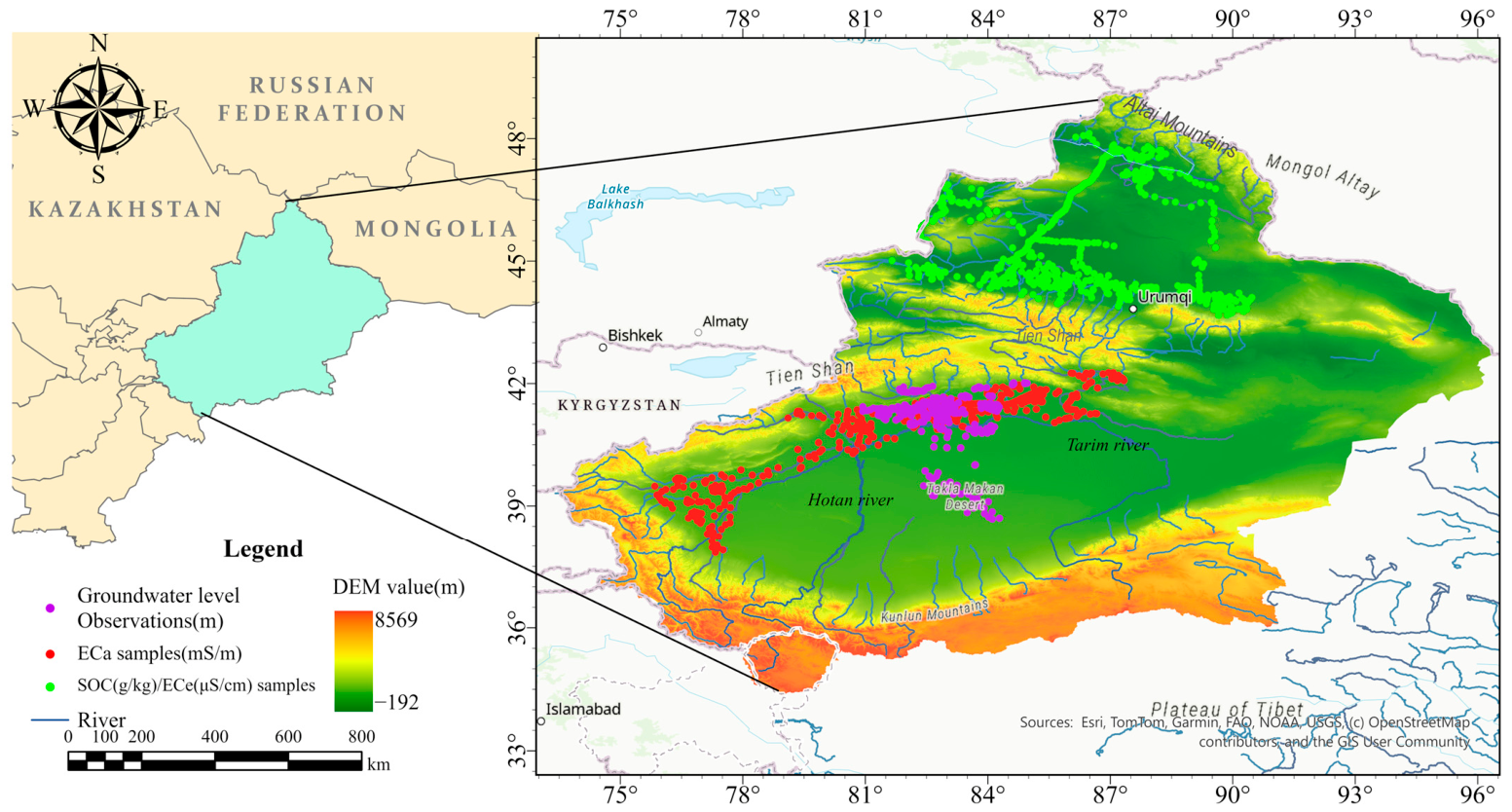
Figure 1. Geographical location of the Xinjiang study area and spatial distribution of sampling sites.
Remotesensing 18 02859 g001
Figure 2. Overall methodological workflow of this study.
Remotesensing 18 02859 g002
Figure 3. Schematic diagrams of the standalone base predictive model architectures constructed in this study, including the (a) LSTM internal control structure, (b) GRU internal control structure, (c) BiLSTM internal control structure, (d) iTransformer encoder architecture, (e) RF ensemble tree structure, and (f) 2D convolutional neural network (CNN) structure.
Remotesensing 18 02859 g003
Figure 4. Schematic architectures of hybrid deep learning models designed for high-dimensional environmental covariates: (a) CNN–RNN framework; (b) CNN–RNN–SE framework with channel-wise feature recalibration; and (c) iTransformer–RNN framework.
Remotesensing 18 02859 g004
Figure 5. Training-loss trajectories of representative deep learning models for ECe and SOC prediction. Panels (ad) show the models used for ECe prediction: (a) INFO–BiLSTM, (b) KOA–CNN–BiLSTM, (c) BSLO–CNN–GRU–SE, and (d) KOA–CNN–LSTM–SE. Panels (eh) show the models used for SOC prediction: (e) SSA–CNN–GRU–SE, (f) RIME–BiLSTM, (g) BSLO–CNN–BiLSTM, and (h) IVY–CNN–GRU–SE.
Remotesensing 18 02859 g005
Figure 6. Training-loss trajectories of representative deep learning models for GWL and ECa prediction. Panels (ad) show the models used for GWL prediction: (a) KOA–BiLSTM, (b) BSLO–CNN–LSTM, (c) AVOA–LSTM, and (d) SSA–CNN–GRU. Panels (eh) show the models used for ECa prediction: (e) HOA–CNN–GRU–SE, (f) SA–CNN–BiLSTM, (g) INFO–CNN–LSTM, and (h) SSA–CNN–GRU–SE.
Remotesensing 18 02859 g006
Figure 7. Ribbon plots illustrating the feature selection results of ten metaheuristic optimization methods. A total of 149 candidate environmental covariates were considered for ECe, SOC, and ECa, whereas 122 candidate covariates were considered for GWL. Colored ribbons indicate that a specific feature was selected by the corresponding algorithm: (a) feature retention for the ECe dataset; (b) feature retention for the SOC dataset; (c) feature retention for the ECa dataset; and (d) feature retention for the GWL dataset.
Remotesensing 18 02859 g007
Figure 8. Sankey diagrams illustrating the preference and contribution weights of ten intelligent optimization feature selection methods across key environmental covariate categories. The ribbon thickness quantifies the relative importance percentage of each feature within the overall retained subset: (a) ECe dataset; (b) SOC dataset; (c) GWL dataset; and (d) ECa dataset.
Remotesensing 18 02859 g008
Figure 9. Bar charts comparing the R2 values of combinations between ten intelligent optimization feature selection methods and five standalone benchmark models (RF, LSTM, GRU, CNN, and BiLSTM): (a) ECe dataset; (b) SOC dataset; (c) GWL dataset; and (d) ECa dataset.
Remotesensing 18 02859 g009
Figure 10. Bar charts comparing the RMSE values of combinations between ten intelligent optimization feature selection methods and five standalone benchmark models (RF, LSTM, GRU, CNN, and BiLSTM): (a) ECe dataset; (b) SOC dataset; (c) GWL dataset; and (d) ECa dataset.
Remotesensing 18 02859 g010
Figure 11. Box plots illustrating the R2 distributions for combinations of ten metaheuristic feature selection methods and eight hybrid deep learning models (including iTransformer and CNN-RNN variants): (a) ECe dataset; (b) SOC dataset; (c) GWL dataset; and (d) ECa dataset.
Remotesensing 18 02859 g011
Figure 12. Box plots illustrating the RMSE distributions for combinations of ten metaheuristic feature selection methods and eight hybrid deep learning models (including iTransformer and CNN-RNN variants): (a) ECe dataset; (b) SOC dataset; (c) GWL dataset; and (d) ECa dataset.
Remotesensing 18 02859 g012
Figure 13. Heatmaps of relative performance enhancement rates for standalone deep learning models and iTransformer-RNN hybrid models compared to the baseline Random Forest (RF). Positive values (yellow-green) indicate superior performance over RF, while negative values (blue) represent performance degradation: (a) ECe dataset; (b) SOC dataset; (c) GWL dataset; and (d) ECa dataset.
Remotesensing 18 02859 g013
Figure 14. Heatmaps of relative performance enhancement rates for CNN-RNN models and CNN-RNN-SE hybrid models compared to the baseline Random Forest (RF). Positive values (yellow-green) indicate superior performance over RF, while negative values (blue) represent performance degradation: (a) ECe dataset; (b) SOC dataset; (c) GWL dataset; and (d) ECa dataset.
Remotesensing 18 02859 g014
Figure 15. SHAP beeswarm plots for the best-performing models of (a) ECe, (b) SOC, (c) GWL, and (d) ECa. Environmental covariates are ranked from top to bottom according to their mean absolute SHAP values. Each point represents one sample, and its horizontal position indicates the magnitude and direction of the contribution of the corresponding covariate to the model output. Red and blue points represent relatively high and low feature values, respectively.
Remotesensing 18 02859 g015
Figure 16. Scatter plots of measured versus predicted values for the top four algorithm combinations with the highest predictive performance in the ECe and SOC datasets: (a) KOA-CNN-BiLSTM; (b) BSLO-CNN-GRU-SE; (c) KOA-CNN-LSTM-SE; (d) KOA-CNN-LSTM; (e) BSLO-CNN-BiLSTM; (f) KOA-CNN-BiLSTM; (g) BSLO-CNN-LSTM; and (h) AVOA-CNN-BiLSTM.
Remotesensing 18 02859 g016
Figure 17. Scatter plots of measured versus predicted values for the four highest-performing algorithm combinations in the GWL and ECa datasets: (a) IVY–CNN–GRU–SE; (b) SSA–CNN–LSTM–SE; (c) INFO–CNN–LSTM–SE; (d) RIME–BiLSTM; (e) INFO–CNN–LSTM; (f) SA–CNN–LSTM; (g) SA–CNN–BiLSTM; and (h) HOA–BiLSTM.
Remotesensing 18 02859 g017
Figure 18. Spatial prediction maps for Northern Xinjiang at a 90 m spatial resolution: (a) ECe predicted by KOA–CNN–BiLSTM and (b) SOC predicted by BSLO–CNN–BiLSTM. The black outline indicates the Northern Xinjiang study-area boundary, and the black points represent the 709 field sampling locations used for ECe and SOC modelling. The colour scales show the predicted ECe (μS/cm) and SOC (g/kg) values, respectively.
Remotesensing 18 02859 g018
Figure 19. Spatial prediction maps for the target-specific study domains in Southern Xinjiang at a 90 m spatial resolution: (a) GWL predicted by IVY–CNN–GRU–SE within the GWL observation and modelling extent and (b) ECa predicted by INFO–CNN–LSTM within the Tarim River Basin sampling and modelling extent. The overlaid points represent the 436 GWL observations and 474 ECa sampling locations, respectively. The colour scales show predicted GWL depth (m) and ECa (mS/m).
Remotesensing 18 02859 g019
Table 1. Summary of the environmental covariates used in the four prediction tasks.
Covariate CategoryRepresentative VariablesNumber of VariablesData Source or Processing
Vegetation-related variablesCI, DVI, EVI, EVI2, GCC, GNDVI, NCI, NDVI, NDWI, NIRV, SAVI, and SR26Median and maximum values derived from Sentinel-2 imagery acquired from 2019 to 2022
Radar variablesVV, VH, and polarization or texture features P1–P1126Median and maximum values derived from Sentinel-1 SAR imagery
Climatic variablesprec, srad, tavg, tmax, tmin, vapr, wind, and bio1–bio1961Monthly climatic and bioclimatic variables obtained from WorldClim 2
Topographic variablesDEM, slope, TWI, TPI, and related terrain indices9Derived using SAGA GIS 9.5.1
Soil physicochemical variablesSoil nutrients, texture, bulk density, porosity, water-related properties, soil colour, OC, pH, and CEC27Mean values calculated across six standard soil depths
Total 149All covariates were resampled to a spatial resolution of 90 m
Note: All 149 covariates were considered for ECe, SOC, and ECa prediction. For GWL prediction, the 27 soil physicochemical covariates were excluded, resulting in a total of 122 candidate covariates. Full definitions of all abbreviations used in this table are provided in Supplementary Table S2.
Table 2. Core hyperparameter configurations of the 13 standalone and hybrid deep learning predictive models constructed in this study, including RF, CNN, RNN variants, and attention-enhanced architectures.
AlgorithmParameter
RFN_estimators(100)
CNNkernel_size(2×1×1), filters(16), conv_stride(1), padding(Valid), pool_size(2×1), pool_stride(1), pool_padding(Valid), activation(ReLU), optimizer(Adam), learning_rate(0.001), batch_size(50), epochs(70), shuffle(True), validation_freq(20)
LSTM/GRUhidden_size(16), num_layers(2), dropout(0.2), activation(Tanh+Sigmoid), optimizer(Adam), learning_rate(0.001), batch_size(50), epochs(70), sequence_length(1), loss(MSE)
BiLSTMhidden_size(16→32), num_layers(2), dropout(0.2), activation(Tanh+Sigmoid), layer1_output(Sequence), layer2_output(Last), merge_mode(Concat), optimizer(Adam), learning_rate(0.001), batch_size(50), epochs(70), sequence_length(1), loss(MSE), shuffle(True), validation_freq(20)
iTransformer—LSTM
iTransformer—GRU
iTransformer—BiLSTM
pos_encoding_len(32), attn_layers(2), heads(1), key_dim(2), hidden_size(16), dropout(0.2), activation(Tanh+Sigmoid), optimizer(Adam), learning_rate(0.001), batch_size(68), epochs(70), sequence_length(1), loss(MSE)
CNN—LSTM
CNN—GRU
CNN—BiLSTM
kernel_size(2×1×1), filters(16), conv_stride(1), padding(Valid), activation(ReLU), pool_size(2×1), pool_stride(1), pool_padding(Valid), hidden_size(16), output_mode(Last), optimizer(Adam), learning_rate(0.001), batch_size(68), epochs(70), shuffle(True), validation_freq(20)
CNN—LSTM—SE
CNN—GRU—SE
kernel_size(2×1×1), filters(16), conv_stride(1), output_channels(32), padding(Valid), activation(ReLU), pool_size(2×1), pool_stride(2), pool_padding(Valid), channel_reduction(16), activation_2(Sigmoid), hidden_size(16), output_mode(Last), optimizer(Adam), learning_rate(0.001), batch_size(68), epochs(70), shuffle(True), validation_freq(20)
Table 3. Descriptive statistics of measured target variables (ECe, SOC, ECa, and GWL) in the Northern Xinjiang and Southern Xinjiang (Tarim River Basin) study areas.
AreaTarget VariablesNumbersMeanMaxMinSDCV (%)
Northern XinjiangECe (μS/cm)7091920.8738,97537.43688.34192.01
SOC (g/kg)7098.1568.760.496.174.76
Southern XinjiangECa (mS/m)474338.131763.941.39375.18110.96
Groundwater level (m)43612.25150.240.7922.89186.86
Table 4. Descriptive summary of predictive performance across different feature-selection methods for the four datasets, including mean values, standard deviations, and coefficients of variation for R2 and RMSE across the evaluated predictive architectures.
DatasetFeature Selection MethodMean R2Mean RMSESDR2SDRMSECVR2 (%)CVRMSE (%)
GWLAVOA0.899.580.073.237.7433.73
BSLO0.947.060.042.624.3337.08
HOA0.936.980.051.965.0628.13
INFO0.956.190.022.012.4232.40
IVY0.937.250.052.565.8335.23
KOA0.947.190.021.192.2016.55
PSO0.938.020.052.814.9535.09
RIME0.946.690.042.194.0732.73
SA0.909.130.063.647.0939.93
SSA0.936.990.062.576.1336.77
ECaAVOA0.58294.730.1441.4624.7214.07
BSLO0.60290.320.1134.7219.2411.96
HOA0.57287.560.1653.4928.4518.60
INFO0.64270.320.1554.5522.5020.18
IVY0.63265.050.1344.8821.2416.93
KOA0.64268.440.1140.9717.3915.26
PSO0.63274.040.1139.8717.9514.55
RIME0.60278.210.1955.9930.8820.13
SA0.64268.040.1448.2021.3117.98
SSA0.63275.130.1138.4717.0613.98
ECeAVOA0.723584.060.09546.4212.6615.25
BSLO0.723527.300.08583.4311.7416.54
HOA0.723511.910.12688.0516.3519.59
INFO0.713631.160.09566.4213.4415.60
IVY0.743433.090.07502.109.2414.63
KOA0.743408.320.08586.9410.8817.22
PSO0.683831.580.10597.5815.2715.60
RIME0.713601.790.09584.4513.1316.23
SA0.723514.720.07492.839.1514.02
SSA0.703611.310.10637.5614.8717.65
SOCAVOA0.574.490.090.5916.5913.22
BSLO0.574.500.100.6318.1514.02
HOA0.554.720.070.5312.8911.21
INFO0.554.780.080.6613.6213.86
IVY0.554.700.080.6114.6612.90
KOA0.534.700.110.7621.3216.13
PSO0.524.830.070.4813.829.86
RIME0.544.680.070.5513.2511.67
SA0.505.060.070.4613.279.13
SSA0.554.600.070.5313.3911.55
Disclaimer/Publisher’s Note: The statements, opinions and data contained in all publications are solely those of the individual author(s) and contributor(s) and not of MDPI and/or the editor(s). MDPI and/or the editor(s) disclaim responsibility for any injury to people or property resulting from any ideas, methods, instructions or products referred to in the content.