Var-ANN Calibration of FY-3C VASS Temperature Profiles: Evaluation over the Tibetan Plateau and Application to WRF Precipitation Simulation

Highlights

What are the main findings?

• The proposed Var-ANN method improves the accuracy of FY-3C satellite temperature profiles, reducing RMSE from 7.30 to 2.11, bias from −4.77 to −0.72, and increasing the correlation coefficient to 0.998 compared with radiosonde observations.
• Assimilating the calibrated temperature data into the WRF model enhances downstream precipitation forecasting over the Tibetan Plateau, achieving threat scores of 66.9% and 66.7% for two typical heavy rainfall cases.

What are the implications of the main findings?

• The Var-ANN framework provides a practical approach for temperature profile calibration over data-sparse regions, using satellite cross-calibration, effectively correcting retrieval errors caused by clouds, satellite zenith angle, and radiative transfer model uncertainties.
• The improved high-resolution atmospheric profiles over data-sparse regions like the Tibetan Plateau can enhance numerical weather prediction and quantitative precipitation forecasting, supporting better understanding of plateau vortex dynamics and downstream convective systems.

Abstract

Accurate information on atmospheric temperature profiles is crucial for improving numerical weather prediction (NWP). However, the harsh environment of the Tibetan Plateau (TP) limits the availability of station observations, which thereby fail to meet the high spatial resolution required for NWP. In this study, we present an integrated framework as an engineering refinement combining the variation method with an artificial neural network (Var-ANN) to calibrate temperature profiles obtained from the Vertical Atmosphere Sounding System (VASS) aboard the polar-orbiting satellite FY-3C. The variation method is first applied to construct a spatially consistent reference field from available station observations, and this field is then used as the training target for a back-propagation neural network that learns the empirical relationship between satellite brightness temperatures and corrected atmospheric temperature. The calibrated temperature profiles were evaluated against independent radiosonde observations and further tested through assimilation into the Weather Research and Forecasting (WRF) model for precipitation simulation over the TP. Results indicate that the Var-ANN calibration reduces the root-mean-square error (RMSE) by approximately 60% and the mean bias from approximately −5 °C to −0.7 °C relative to radiosonde observations. In two WRF case studies, the calibrated profiles show potential for improving precipitation forecast skill, although the limited sample size precludes robust conclusions about operational forecast improvements. The Var-ANN framework provides a practical approach for enhancing the utility of FY-3C VASS temperature products for NWP applications over data-sparse complex terrain.

1. Introduction

The accuracy of numerical weather prediction (NWP) is highly reliant on the quality of initial atmospheric state fields. This is especially critical over the Tibetan Plateau (TP), where weather and climate exert significant impacts on downstream regions and where conventional observations are sparse. Satellite-derived temperature profiles offer a promising source of spatially continuous information, but their accuracy is limited by retrieval errors associated with cloud contamination, surface emissivity uncertainty [1], and radiative transfer assumptions, particularly over complex terrain. Various approaches have been developed to improve satellite retrieval accuracy, including variational bias correction, machine-learning-based calibration, and hybrid methods combining physical constraints with statistical learning. This study builds upon these prior efforts by integrating variational quality control with neural network regression specifically for FY-3C VASS temperature profiles over the TP—a combination of product and region for which such calibration has not been previously demonstrated.

Recognized as best capturing the actual atmospheric conditions, radiosonde observations were directly assimilated into NWP models in early studies, leading to evident improvements in prediction skills [2,3,4].However, with the continuous advancement of high-resolution NWP, the insufficient station density of sounding data over the TP poses challenges for its assimilation in fine-scale numerical simulations. Therefore, some studies have attempted to assimilate satellite observations, which have broader spatial coverage, to improve the accuracy of high-resolution precipitation simulations [5,6,7,8]. However, it was found that discrepancies still existed between satellite retrievals and sounding observations [9,10,11], since satellites do not directly measure atmospheric profiles but indirectly retrieve them through atmospheric radiative transfer models.

Prior ML-based satellite temperature calibration studies have primarily (i) relied on direct satellite-radiosonde collocation pairs for training, which are sparse over complex terrain; (ii) been trained on the original retrieval without a physically constrained reference; or (iii) focused on global or mid-latitude regions without addressing the specific challenges of the Tibetan Plateau (strong surface heterogeneity, limited station density, systematic cold bias in IR-based retrievals). The Var-ANN framework addresses these gaps by using variationally corrected fields to construct a spatially consistent training dataset and by optimizing the calibration specifically for FY-3C VASS over the TP. To reduce inaccuracies in satellite observations, several studies directly assimilated brightness temperatures from atmospheric radiative transfer models [12,13]. This method imposes indirect constraints on the atmospheric structure but lacks validation from surface observations. Hence, it is highly dependent on the accuracy and stability of the observation instrument. Another approach involves pre-correcting satellite retrievals with radiosonde data prior to assimilation into NWP models. This not only ensures the consistency between satellite and sounding data but also maintains the high-resolution characteristics of satellite observations. The variation method is one of the representative methods, which can minimize the value of the Euler equation in the error field by constructing a functional function. This method can greatly reduce data errors and has been widely adopted for satellite data correction and model assimilation studies [14,15,16]. Traditional variational approaches have limited effectiveness in correcting discrete observation fields, since error propagation is confined to small regions under high-resolution grid settings. Local errors caused by nonlinear variables, such as satellite elevation angles in the retrieval process, are also hard to compensate for via variational methods [17,18,19,20,21]. Thus, this study develops a hybrid Var-ANN method integrating variational schemes and artificial neural networks to obtain a more precise high-resolution dataset, which benefits research into the dynamic and thermal structure over the TP. The accuracy of the dataset is also confirmed by improved simulations of downstream precipitation. As numerical models continue to advance toward finer scales, higher requirements are placed on observational data, making high-accuracy, high-resolution satellite data essential for addressing this issue.

2. Data and Method

2.1. Study Area

The study area covers the Chinese mainland (70°E–140°E, 10°N–60°N). The FY-3C satellite passes over this region at 0000 and 1200 UTC, consistent with the observation times of conventional meteorological stations. This region features complex weather, climate, and topographic conditions, which pose considerable challenges to atmospheric temperature profile retrieval. The selection of study period was determined by considerations of sample size and practical significance. The research period covers July–August 2019, since summer clouds are more frequent and impose greater interference on temperature profile retrieval. As radiative transfer models (RTM) have become increasingly capable with enhanced retrieval and correction algorithms, the most recent 2019 dataset is employed.

This study focuses on the summer season (June–August) for three reasons. First, the Tibetan Plateau’s thermal forcing on downstream precipitation is most pronounced during summer, when heavy rainfall events and associated secondary disasters (floods, landslides) are most frequent over the Yangtze River Basin and eastern China. Second, operational weather forecasting in this region prioritizes summer quantitative precipitation prediction due to the socio-economic impacts of summer flooding. Third, the FY-3C VASS temperature retrieval exhibits its largest cold bias during summer over the TP, making this season the most critical target for calibration efforts. While the calibration model is trained solely on summer 2019 data, cross-seasonal validation using winter 2019/2020 data is presented in the Discussion (Section 4) to assess generalizability.

2.2. Data

This study uses VASS temperature profiles and brightness temperatures (FY-3C) as the main background data for neural network training, supplemented by cloud amount and spatial location information. VASS employs both microwave and infrared measurements to retrieve atmospheric temperature profiles. FY-3C is equipped with three temperature-retrieval-related sensors: the microwave humidity sounder (MWHS), the microwave thermometer sounder (MWTS) and the infrared atmosphere sounder (IRAS). Given the short service life of MWTS (only 2013–2015), VASS products are mainly produced using MWHS and IRAS. MWHS includes fifteen channels: five at 183.31 GHz (water vapor absorption), eight at 118.75 GHz (oxygen absorption), and two window channels at 89 and 150 GHz, respectively. IRAS measures infrared radiative emission from the surface and atmosphere across 26 channels spanning 669–6098 cm⁻¹. Given the impact of clouds, cloud cover products by visible and infrared radiometer (VIRR) onboard FY-3C are adopted. VIRR has seven visible/near-infrared and three infrared bands with a 1.1 km ground resolution, and the cloud products are collocated to the 17 km VASS pixels (http://satellite.nsmc.org.cn, accessed on 7 August 2026). Quality control of the input data is essential to ensure a reliable training process and valid results. To remove outliers and prevent overfitting, we used the middle 50% of the data as the input to the Var-ANN, discarding the upper and lower 25% of extreme values. The dataset was then divided into three parts: 80% for model training, 10% for testing, and 10% for validation.

Temperature profile data from 121 radiosonde stations and 2400 meteorological stations in China were employed to assess the calibration results. These observations were taken at 0000 and 1200 UTC, matching the overpass time of FY-3C. The vertical temperature profiles are interpolated into the RTM pressure levels, covering 1013.25 hPa down to 0.1 hPa across a total of 43 levels.

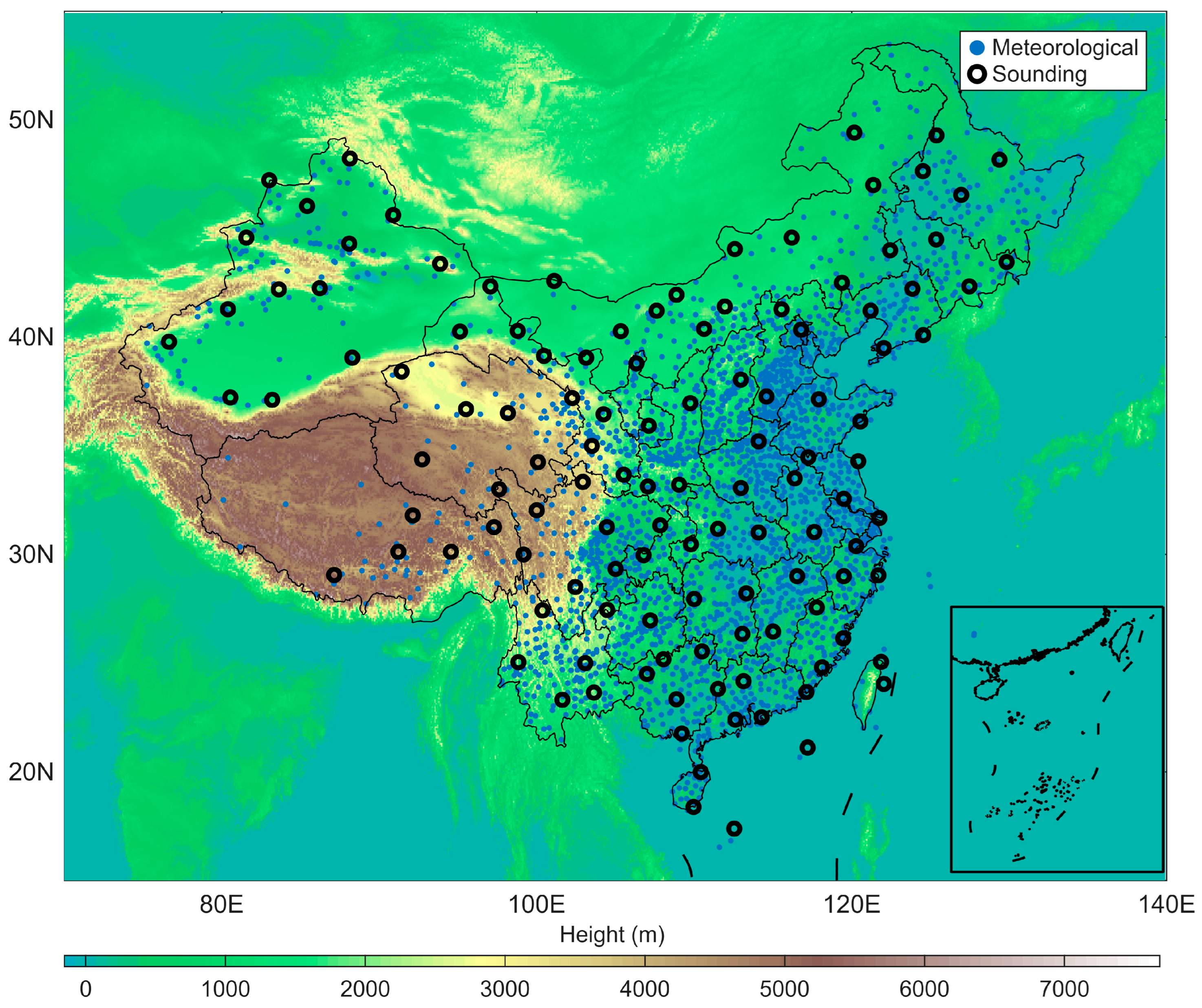
It should be noted that the density of meteorological and radiosonde stations exhibits pronounced east-west heterogeneity across the study domain (Figure 1). The eastern Tibetan Plateau has much denser station coverage due to lower elevation and greater accessibility, while the western TP (above approximately 4500 m) is sparsely instrumented. Consequently, evaluation statistics (RMSE, bias, CC) are inherently weighted toward the eastern region where more satellite–station collocation pairs are available. To address this, evaluation results are stratified by elevation bands (low: 0–2000 m; middle: 2000–4000 m; high: >4000 m) where feasible, and the variation correction step (Section 2.3) operates on a regular grid covering the entire domain, providing a spatially consistent first-guess correction even in data-sparse areas. Performance metrics over the western TP should be interpreted with caution due to smaller sample sizes.

2.3. Variation Method

The variation method is based on the principle that functional functions with multiple independent variables (1) must satisfy the Euler Equation (2).

$$J[U(x,y)]={\iint }_{G}F(x,y,U,{\displaystyle \frac{\partial U}{\partial x}},{\displaystyle \frac{\partial U}{\partial y}})\mathrm{d}x\mathrm{d}y$$

(1)

$$Fu-({\displaystyle \frac{\partial }{\partial x}}F{u}_x+{\displaystyle \frac{\partial }{\partial y}}F{u}_y)=0$$

(2)

For this study, the satellite-derived temperature is set as $T_{Sat}(x,y)$, the corresponding station observation field is $T_{Obs}(I,J)$, and the difference between the two is the error field $\tilde{C}r(I,J)$.

$$\tilde{C}r(I,J)=T_{Sat}(I,J)-T_{Obs}(I,J)$$

(3)

Since station observations are discontinuous across the VASS product grid, $\tilde{C}r(I,J)$ only covers grid points with available in-situ measurements. Thus, it is necessary to construct a more generalized error field function $Cr(x,y)$ and minimize this new function using the variational method.

$$J^{\mathrm{*}}={\iint }_{\mathrm{D}}{(Cr-\tilde{C}r)}^2\mathrm{d}x\mathrm{d}y\to \mathrm{m}\mathrm{i}\mathrm{n}$$

(4)

For this variation problem, a functional function $J^{\mathrm{*}}$ can be constructed as follows:

$$J^{\mathrm{*}}=[\iint (Cr-\tilde{C}r{)}^2+\lambda [{({\displaystyle \frac{\partial Cr}{\partial x}})}^2+{({\displaystyle \frac{\partial Cr}{\partial y}})}^2]]\mathrm{d}x\mathrm{d}y$$

(5)

where $\lambda$ is the constraint coefficient, and the above formula can be rewritten into the following difference scheme:

$$\delta J=\sum \sum [(Cr-\tilde{C}r{)}^2+\lambda [{({\displaystyle \frac{\partial Cr}{\partial x}})}^2+{({\displaystyle \frac{\partial Cr}{\partial y}})}^2]]=0$$

(6)

The corresponding Euler equation is as follows:

$$(Cr-\tilde{C}r)-\tilde{\lambda }({\displaystyle \frac{{\partial }^{2}Cr}{\partial x^2}}+{\displaystyle \frac{{\partial }^{2}Cr}{\partial y^2}})=0$$

(7)

The numerical solution of the above equation is derived through iterative expansion, yielding the variation-corrected temperature field as follows:

$$T\left(x,y\right)=T_{Sat}+Cr(x,y)$$

(8)

2.4. Back-Propagation Artificial Neural Network

An artificial neural network (ANN) is a nonlinear function that approximates the statistical relationship between input and output data. An ANN typically consists of three components: neuronal nodes, an activation function, and the error back-propagation (BP) algorithm. The node values represent the neuron weights, which are continuously updated during training until the output is accurately fitted. The activation function maps neuronal inputs to outputs, enabling the Var-ANN to approximate nonlinear functions. As the core training component, the error back-propagation algorithm iteratively propagates output errors back to each layer’s nodes until the error falls within a predefined threshold. In the Var-ANN model, the weight function adopts the dot-product weight function, the training function is the Levenberg–Marquardt algorithm, the transfer function is the hyperbolic tangent function, the learning function is the gradient descent algorithm, and the performance function is the mean square error. The feedforward neural network was implemented using the Deep Learning Toolbox in MATLAB R2019b. The network was constructed with the feedforwardnet function and trained with the trainlm function. (https://ww2.mathworks.cn/help/deeplearning/ref/feedforwardnet.html, accessed on 7 August 2026).

2.5. Weather Research and Forecasting (WRF) Model

In this study, the WRF model (version 4.1.0) was employed to investigate the improvements of the calibrated dataset in simulating potential vorticity (PV) and predicting downstream precipitation. The WRF simulations were driven by the NCEP-GFS dataset. WRFDA-3DVAR was used to assimilate the calibrated data into the initial WRF fields. To ensure a controlled experimental setup, identical parameterization schemes were adopted across all comparative experiments, as detailed in

Table 1. Parameterization scheme of Weather Research and Forecasting (WRF).

Physical Process	Parameterization Scheme	Reference
Microphysics	Purdue Lin	[22]
Cumulus parameterization	Kain–Fritsch	[23]
Shortwave radiation	Dudhia	[24]
Shortwave radiation	RRTM	[25]

.

2.6. Evaluation Method

Three statistical indicators are employed to evaluate Var-ANN calibration results: the correlation coefficient (CC), root mean square error (RMSE), and bias. These indicators can be calculated as follows:

$$\mathrm{C}\mathrm{C}={\displaystyle \frac{{\sum }_{i=1}^n(x-\overline{x})(y-\overline{y})}{\sqrt{{\displaystyle {\sum }_{i=1}^n}{(x-\overline{x})}^2}\sqrt{{\displaystyle {\sum }_{i=1}^n}{(y-\overline{y})}^2}}}$$

(9)

$$\mathrm{R}\mathrm{M}\mathrm{S}\mathrm{E}={\displaystyle \frac{{\sum }_{i=1}^n{(x-y)}^2}{n}}$$

(10)

$$\mathrm{B}\mathrm{i}\mathrm{a}\mathrm{s}={\displaystyle \frac{{\sum }_{i=1}^n(x-y)}{n}}$$

(11)

In Equations (9)–(11), $x$ denotes the true temperature observed by radiosonde stations, and $y$ denotes the satellite-derived temperature.

Threat Score (TS, also referred to as Critical Success Index, CSI), missing rate (MR), and false alarm rate (FAR) are employed to further evaluate the WRF precipitation simulation. Listed in

Table 2. Evaluation method for precipitation simulation.

Name	Short Name	Calculation	Ideal Value
Threat Score	TS	${\displaystyle \frac{n_{11}}{n_{11}+n_{10}+n_{01}}}$	1
Missing Rate	MR	${\displaystyle \frac{n_{01}}{n_{01}+n_{00}}}{\displaystyle \frac{n_{01}}{n_{11}+n_{01}}}$	0
False Alarm Rate	FAR	${\displaystyle \frac{n_{10}}{n_{11}+n_{10}}}$	0

are the calculation methods for these indicators, which are commonly applied in the simulation evaluation. “Hit” indicates that precipitation is observed by the gauge and also predicted for the same grid points; TS (Threat Score, also referred to as Critical Success Index) quantifies the fraction of correctly predicted observed events (TS = $n_{11}$/($n_{11} + n_{10} + n_{01}$)). FAR is calculated as $n_{10}$/($n_{11} + n_{10}$), representing the proportion of predicted events that are false alarms $n_{11}$.

$n_{10}$ is called “False,” denoting that precipitation is predicted but with no observed record; $n_{01}$ is called “Miss,” signifying that precipitation is observed by the gauge but not predicted; $n_0$ suggests that neither the gauge nor the prediction shows precipitation.

3. Results

3.1. Temperature Profile Correction Results

Many satellite products are retrieved using various artificial intelligence and deep learning methods [26]. The core issue lies in how to construct the training dataset to capture the relationship between input and output data. The FY-3C VASS product combines microwave observations (MWTS and MWHS) and infrared measurements to retrieve atmospheric temperature profiles. The Var-ANN calibration framework uses variationally corrected station observations as the training target, thereby learning an empirical correction function that maps the original VASS retrievals toward more accurate temperature estimates. We emphasize that the improvements reported below should be understood as verification that the calibration successfully reduces systematic retrieval biases (a quality assurance outcome), rather than as discoveries of new atmospheric phenomena. The improvements in RMSE and bias reported below should be interpreted as evidence of successful calibration—i.e., quality assurance confirming that the Var-ANN framework effectively learns the empirical relationship between satellite brightness temperatures and atmospheric temperature profiles, as expected from supervised statistical calibration—rather than as new scientific discoveries about atmospheric processes.

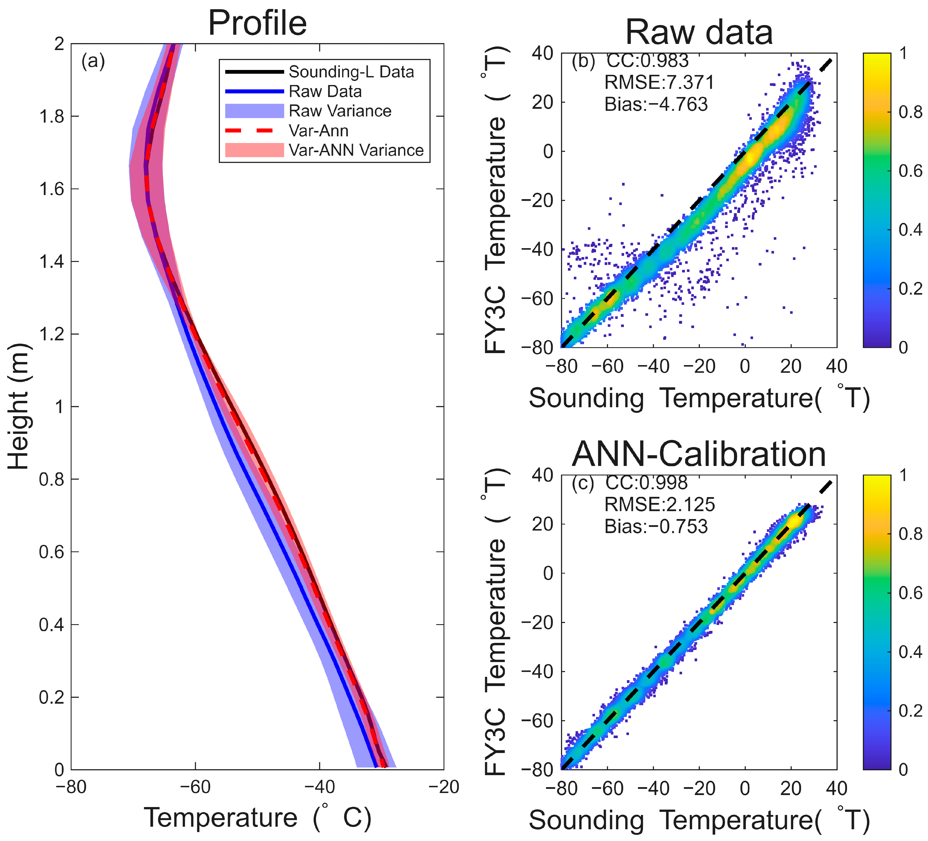
As shown in Figure 2a, the bias at high temperatures (approximately 7–27 °C) and low temperatures (around −83 to −43 °C) is smaller than that at mid-level temperatures, indicating that temperature retrievals in the upper and lower atmosphere are more accurate than in the middle atmosphere (Figure 2a). Scatter plots between satellite and radiosonde observations demonstrate that the calibrated dataset exhibits improved accuracy. Outliers deviating from the scatter distribution have been corrected, and the data points now cluster more closely around the linear relationship between satellite retrievals and station observations. Relative to radiosonde measurements, the calibrated satellite data yields an RMSE of 2.11, a bias of −0.72, and a correlation coefficient (CC) of 0.998, all of which represent significant improvements over the original satellite data (7.30, −4.77, and 0.984, respectively). The Var-ANN model has been constructed to characterize the relationship between brightness temperature and atmospheric temperature. Vertical temperature retrieval relies on contributions from the vertical atmospheric structure, which exhibits stable climatic characteristics. The retrieval algorithm establishes regression relationships based on these stable features, which are encoded in the parameters of radiative transfer model equations. Accordingly, Var-ANN calibration not only improves low-quality temperature retrievals but also preserves the accuracy of high-quality data.

The results indicate that the VASS temperature profile is colder than the station observations throughout the entire atmosphere, particularly in the middle and lower troposphere (0–12 km), a region closely linked to atmospheric dynamic and thermodynamic structures. Negative biases arise from multiple factors, including observational calibration uncertainties and the RTM performance as well as aerosol effects [27]. Although the bias is significantly reduced following Var-ANN calibration (from −4.77 in the raw data to −0.72), a residual bias remains unavoidable when training the network solely with VASS data. Notably, data quality at 0000 UTC (8 a.m. BJT) exhibits marked improvement compared to 1200 UTC (8 p.m. BJT). The increased fluctuations at 1200 UTC are likely to be attributable to orbital biases, a well-documented characteristic of the FY-3C microwave radiation imager [28].

The systematic cold bias in VASS temperature profiles throughout the entire atmospheric column can be attributed to several factors. First, the VASS retrieval algorithm relies on infrared channels that are sensitive to cloud-top emission; under cloudy conditions, the retrieved temperature is biased toward the colder cloud-top brightness temperature rather than representing the full-column atmospheric temperature. Second, surface emissivity uncertainty over the complex TP terrain, with highly variable snow cover, ice, and bare soil, introduces errors in the radiative transfer model’s assumptions, particularly affecting lower-tropospheric retrievals. Third, the MWHS channels operating in the 183.31 GHz water vapor absorption band are sensitive to humidity variability, which can introduce systematic biases in the mid-troposphere under moist convective conditions. The Var-ANN calibration addresses these biases by learning the empirical relationship between satellite radiances and in situ radiosonde observations, effectively reducing the mean cold bias from approximately −5 °C to −0.7 °C (

Table 3. Standard deviation (Std.), root mean square error (RMSE) and bias relative to sounding observations at each atmospheric level.

Isobaric Level		Raw Data			Var-ANN
No.	Height (m)	Std.	Bias.	RMSE	Std.	Bias.	RMSE
1	0	8	−4.5	11.22	2.3	−0.49	1.63
2	65.25	7.81	−3.9	9.92	2.49	−0.45	1.79
3	230.2	7.64	−3.66	9.23	2.5	−0.41	1.97
4	474.95	7.51	−4.02	8.9	2.51	−0.5	2.2
5	784.19	7.31	−4.66	8.91	2.48	−0.65	2.35
6	1146.51	6.94	−4.98	8.71	2.47	−0.73	2.38
7	1553.09	6.39	−5.16	8.24	2.4	−0.75	2.34
8	1997.17	5.87	−5.03	7.63	2.33	−0.75	2.14
9	2473.8	5.52	−4.95	7.2	2.34	−0.76	2.03
10	2979.43	5.33	−5.08	7.03	2.43	−0.78	1.96
11	3511.79	5.28	−5.5	7.21	2.61	−0.84	1.91
12	4069.59	5.41	−5.9	7.48	2.77	−0.91	1.92
13	4652.11	5.65	−6.25	7.79	2.94	−0.94	1.9
14	5259.54	5.75	−6.81	8.23	3.13	−1.02	1.9
15	5892.34	5.8	−7.27	8.54	3.41	−1.07	1.95
16	6551.03	5.68	−7.61	8.75	3.69	−1.14	2.05
17	7236.79	5.4	−7.89	8.89	3.91	−1.22	2.16
18	7950.11	5.07	−7.81	8.78	4.07	−1.25	2.25
19	8691.55	4.63	−7.06	8.12	4.02	−1.17	2.26
20	9461.6	4.01	−5.86	7.17	3.49	−1.04	2.31
21	10,260.27	3.41	−4.77	6.22	2.45	−0.87	2.36
22	11,087.37	3.12	−3.67	5.21	1.5	−0.68	2.36
23	11,943.06	3.23	−2.35	4.04	2.45	−0.45	2.18
24	12,829.77	4.35	−0.98	3.59	4.12	−0.19	1.97
25	13,744.08	5.73	−0.33	3.99	5.62	−0.08	1.91
26	14,684.76	6.77	−0.03	4.5	6.67	−0.06	1.9
27	15,675.75	6.76	−0.36	4.37	6.62	−0.09	1.94
28	16,643.1	6.31	−1.78	4.4	5.29	−0.29	1.79
29	17,659	5.16	−1.95	3.94	3.82	−0.3	1.66
30	18,701.29	4.04	−0.47	2.68	2.85	−0.06	1.52
31	19,775.01	3.51	1.4	2.79	2.39	0.25	1.59
32	20,884.27	3.66	2.62	3.91	2.02	0.41	1.73
33	22,033.02	4.84	3.42	5.61	1.71	0.54	1.99
34	23,227.87	5.42	4.05	6.5	1.91	0.59	2.35
35	24,473.4	6	4.02	7.27	2.39	0.55	2.72
36	25,773.19	5.94	0.93	8.58	1.93	0.2	3.16
37	27,131.4	6.57	4.67	11.62	3.23	0.6	4.71
38	28,556.77	7.25	10.71	16.55	4.62	1.62	5.86
39	30,049.14	7.77	17.16	18.61	5.29	4.36	6.27
40	31,608.46	5.63	24.48	24.48	6.6	4.23	4.23
41	33,236.83	2.67	13.07	13.07	7.05	1.9	1.9
42	34,918.84	3.27	−6.11	6.1	9.95	−1.43	1.42
43	36,639.07	8	−4.5	11.22	2.3	−0.49	1.63

Unit: Meter for Height, °C for Std., Bias, and RMSE.

). Residual biases can be further reduced in future work by incorporating cloud-type-specific correction factors, integrating additional predictors such as cloud-top pressure and optical depth, or applying a physically constrained radiative transfer bias correction as a pre-processing step.

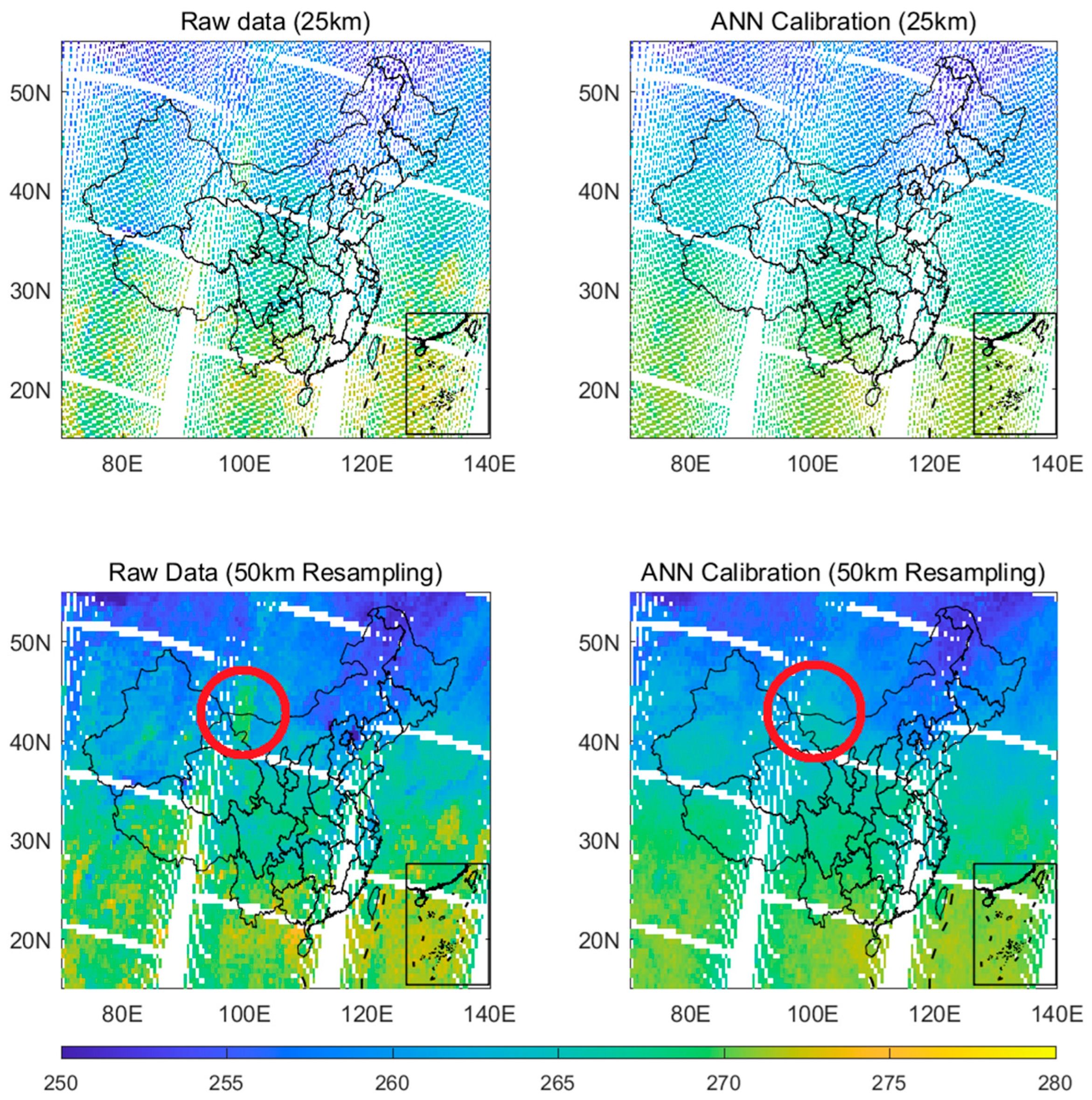
Despite the overall accuracy of temperature data, discontinuous regions appear at the edge of the satellite swath, which are clearly visible in the spatial distribution (Figure 3). Because of the coarser resolution at the swath edge, we resampled the data to 50 km resolution to highlight these discontinuities. The IRAS instrument records 56 pixels per scan line, and anomalous data typically occurred periodically at approximately the 10th to 15th pixel (from left to right), persisting across about 10 consecutive scan lines. Such highly regular scan-line anomalies clearly do not represent real atmospheric signals and thus constitute a major source of error. Traditional methods for addressing this issue apply spatial smoothing over the entire domain (commonly five-point or nine-point smoothing), at the cost of degrading high-resolution features. In contrast, after Var-ANN correction, the swath edges become significantly smoother while preserving most of the high-resolution information.

Temperatures at various isobaric levels over the study period were analyzed (Table 3). It can be observed that upper-atmosphere temperatures exhibit a branch that is higher than radiosonde observations (Figure 2c), a feature that becomes more pronounced in the calibrated data. These results indicate that the Var-ANN model captures two types of relationships. One is strongly positively correlated with station temperatures (the diagonal dashed line in Figure 2), consistent with real atmospheric conditions. The other regression behavior is irregular; temperatures in the middle and lower atmosphere are underestimated but those in the upper atmosphere are overestimated. This may be attributed to MWHS channels located in water vapor absorption bands. Under cloudy conditions, higher water vapor content can cause the Var-ANN model to misjudge the vertical level of temperature signals, leading to underestimated retrievals in the middle and lower troposphere and overestimated values within the temperature inversion layer (−53 to −33 °C). Owing to the greater vertical variability in the temperature inversion layer, the upper-atmosphere branch is more distinct, as clearly reflected in the vertical temperature profiles (Figure 2). In addition to the regression branching, the negative bias is substantially reduced but still remains, with a value of −0.72 °C. This result is reasonable, given that the calibration method relies solely on FY-3C satellite observations and is independent of radiosonde data. To further eliminate this bias, additional temperature profile data are required, which can be obtained through inter-calibration with other satellites.

3.2. Design and Description of Var-ANN

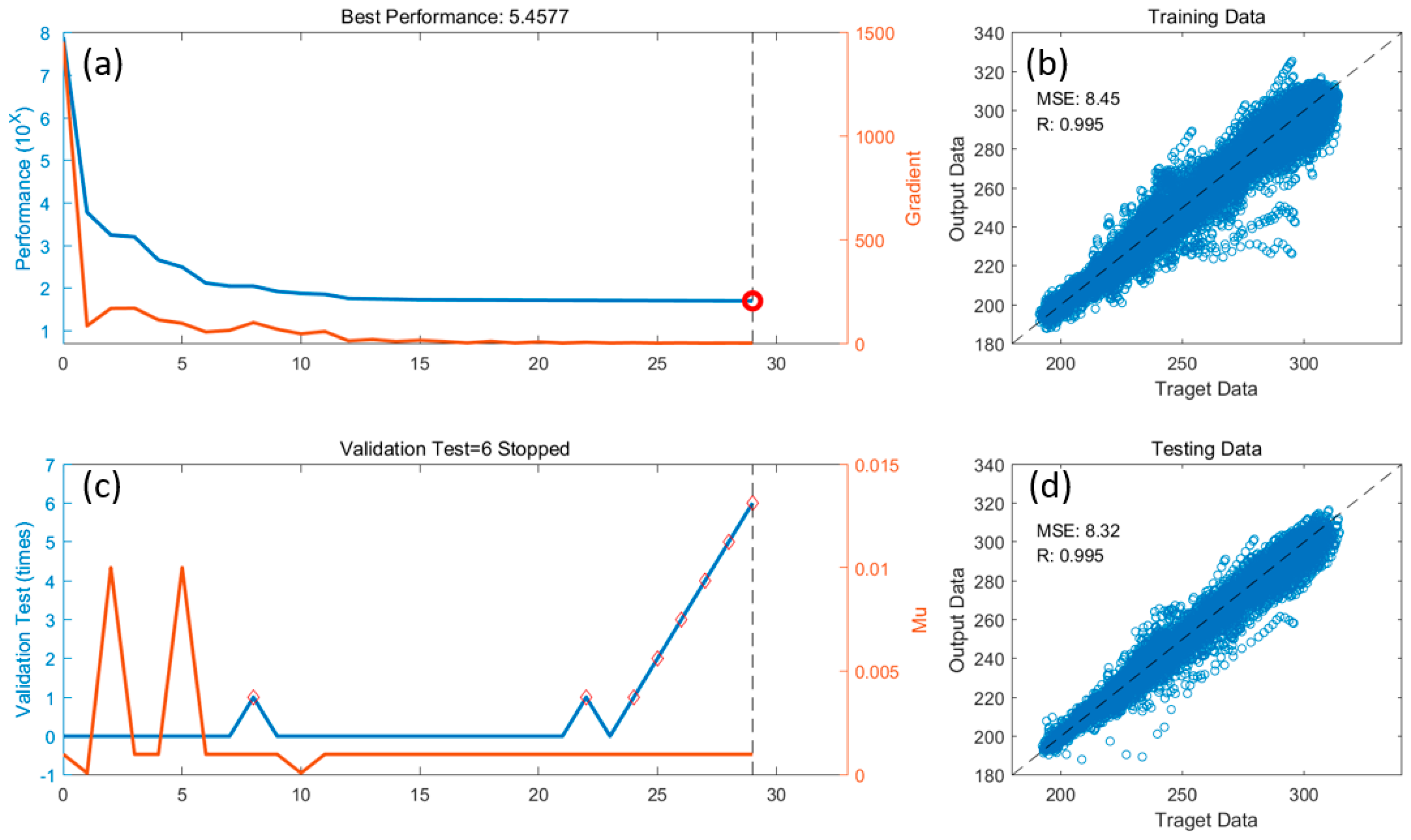
The structure of the Var-ANN model is often determined subjectively, lacking sufficient theoretical and physical support. In this study, we trained and tested several Var-ANN architectures with different configurations, aiming to achieve a more objective network design. We adopted a Var-ANN with two hidden layers, where the number of nodes in each layer was set to 20. Here, representative results are presented in Figure 4. These results indicate that a simple network structure cannot adequately characterize the relationship between brightness temperature and atmospheric temperature. As the network architecture becomes more complex, the ability of Var-ANN to represent this relationship improves, although at the cost of increased computational cost for training. Once the model capacity reaches its upper limit, further increasing the number of nodes no longer improves the model performance. The redundant nodes remain involved in training but contribute little to the final output. The number of training samples also requires careful tuning. Insufficient training samples prevent the model from adequately capturing the underlying relationship, while an excessively large sample size leads to overfitting of the temperature profiles. An over fitted Var-ANN tends to store individual sample details within each node, resulting in ineffective correction of the output temperature profiles. After considering the above factors, we finalized the Var-ANN structure (six nodes in the first layer and five nodes in the second layer) and selected the training period (summer 2019).

Training data play an essential role, as they endow the Var-ANN with physical meaning and link it to atmospheric mechanisms. The output dataset consists of the 43-level temperature profiles retrieved by VASS, which represent the results of the RTM employed in the VASS system. The input data are composed of three parts, with the primary part being the brightness temperatures observed by fifteen MWHS channels. Although these channels are designed for water vapor sounding, their radiative frequency information can still be utilized for temperature calibration. Cloud cover retrieved by VIRR is also included as input to mitigate inaccuracies in the RTM under cloudy conditions. In addition to satellite radiance measurements, the longitude and latitude of each observed pixel are also incorporated into the input dataset as geographic information. Each input component carries distinct physical significance related to atmospheric temperature and RTM. Specifically, MWHS data contain integrated atmospheric information, which conventional RTMs rely on to retrieve temperature profiles. The inclusion of cloud cover enables the Var-ANN to characterize the radiation–temperature relationship under cloudy conditions. This relationship remains poorly constrained and cannot be accurately represented by RTMs [29], which constitutes a major source of error in remote sensing observations. Many local factors also exert considerable influence on temperature profile retrieval, such as aerosols, atmospheric circulation, and land cover. These factors involve complex interaction mechanisms and are highly location-dependent. Therefore, longitude and latitude are also used as input data to approximately represent the influences of these local variables. Such auxiliary pixel information enables the Var-ANN model to consider the effects of local factors.

The training process is illustrated in Figure 4, which summarizes the overall fitting procedure and performance. The error gradient decreased steadily throughout training, indicating that the Var-ANN solution was converging. The performance is evaluated using the mean squared error (MSE), which measures the discrepancy between the network-output temperatures and the original VASS temperatures. The MSE dropped rapidly in the early stage of training. As the Var-ANN gradually approached the temperature relationship, the rate of decrease slowed and eventually stabilized at epoch 29, with an optimal MSE of 5.45. The MU parameter is related to machine precision and iterative error. It increases whenever an iteration leads to a higher error. Validation testing used 10% of the input data to verify the model output, with the MU increasing continuously each time the validation error increased. Training terminated if the MU exceeded 10⁵ or the number of validation failures exceeded 6. These two parameters constrain the training process within reasonable boundaries, ensuring that the Var-ANN properly captures the underlying features.

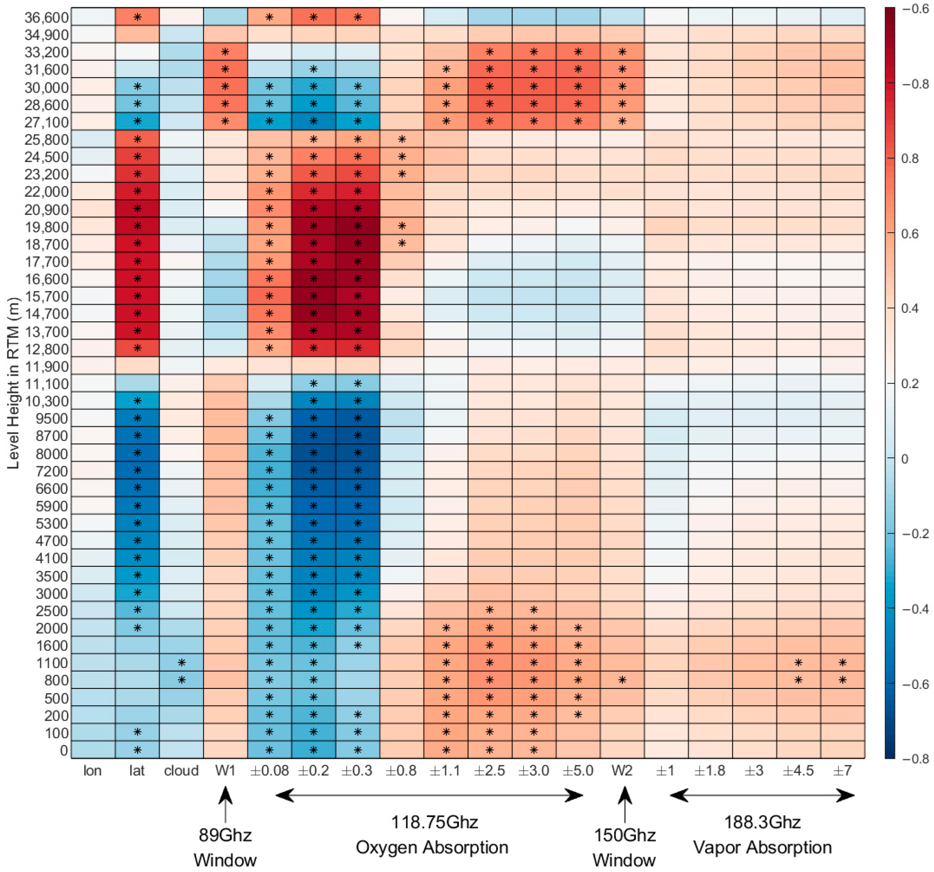
Var-ANN encodes its input-to-output processing procedure through node values, which poses challenges for interpretation. However, the contribution of input to the output has been captured through correlation analysis, with the results presented in Figure 5. It is noteworthy that latitude is highly correlated with the temperature profile and exerts different effects on the stratosphere and troposphere. Specifically, the tropospheric temperature is heated by surface radiation, while the surface itself is heated by solar radiation. As higher latitudes receive less solar radiation, a negative correlation exists between latitude and tropospheric temperature. With the increase of altitude, the temperature is less affected by the surface and more influenced by temperature advection. The study area of this article is mainly located in the middle latitude region, which is controlled by the Ferrel circulation. Consistent with known climatology, this circulation pattern transfers heat from high latitude to low latitude, resulting in a positive correlation in the stratosphere. The correlation with longitude is similar to that with latitude but not statistically significant. The negative correlation in the lower atmosphere is the result of the synergy between the heating effect of the TP and the westerlies; the TP heats the temperature of the lower atmosphere, while the westerlies transport this heat eastward. In contrast, the positive correlation in the stratosphere is caused by the westward component of the Ferrel circulation. The research results demonstrate the necessity of additional geographical information to enable Var-ANN to extract surface–atmosphere coupling features and circulation characteristics, thereby further correcting the temperature profile in line with local conditions.

Clouds show a negative correlation with the output across most levels, though this relationship is weak and non-significant. This indicates that Var-ANN fails to fully capture cloud-related features in the RTM. Although clouds do not absorb microwave radiation, refraction and scattering still occur, lowering observed brightness temperature and, in turn, retrieved temperature. Despite this weak linkage, the model still partially corrects cloud-induced error, especially in the lower atmosphere (882.8 hPa and 922.5 hPa). The unique predominance of negative cloud correlations across most levels suggests that cloud parameters could be an effective means of mitigating negative biases in station observations (Figure 2). To assist RTM, two window channels operating at 89 GHz and 150 GHz are designed to capture surface radiation parameters. The oxygen absorption channel (118.75 GHz) serves as the primary component for retrieving temperature profiles, with its narrow pass-bands (width ≤ 0.3 GHz) exhibiting a high correlation with almost all pressure levels. In contrast, the wide pass-bands (width > 0.3 GHz) are highly correlated with the temperatures of the upper and lower atmospheres, which supplements the levels where the narrow pass-bands show non-significant correlations. The water vapor absorption channel (183.75 GHz) is designed to observe humidity profiles. The positive features extracted by Var-ANN are consistent with the Clausius–Clapeyron (C-C) equation, which states that an increase in temperature leads to a corresponding increase in specific humidity. This finding demonstrates the functional efficacy of water vapor channels in correcting temperature profiles. The cloud and water vapor channels exert analogous roles within the Var-ANN framework, both displaying comparable correlation patterns with temperatures across nearly all pressure levels. This seemingly contradictory situation affords the Var-ANN two complementary perspectives for characterizing the influence of water on temperature, one rooted in radiative transfer processes and the other in atmospheric thermodynamics. Collectively, these findings demonstrate that the Var-ANN is capable of capturing the fundamental relational characteristics between atmospheric profiles and brightness temperature, mirroring the operational logic of the RTM. Thus, the trained model accurately retrieves temperature profiles, providing more reliable data input for follow-up research.

It is important to note that the correlation-based input–output analysis presented above does not establish causal relationships or reveal mechanistic atmospheric processes. The relationships shown in Figure 5 primarily reflect associations present in the training data and should be interpreted as descriptive summaries of the neural network’s learned input-output mapping, rather than as discoveries about atmospheric behavior. Many of the observed correlations are consistent with well-established physical principles. The meridional temperature gradient with latitude reflects the large-scale thermal structure of the Tibetan Plateau documented by Xu et al. [30] and Zhao et al. [31]; the negative cloud–temperature relationship at lower levels is consistent with infrared radiative transfer theory, whereby clouds reduce observed brightness temperature in IR channels [29]; and the water vapor–temperature covariance aligns with moisture–temperature coupling characteristics over the TP reported by Yang et al. [32]. The analysis serves to characterize the model’s internal representations and to identify which input variables most strongly influence the calibration output, which is useful for model interpretation and potential simplification, but it does not constitute an independent scientific investigation of atmospheric processes.

3.3. Calibrated Data Validation in Data Assimilation

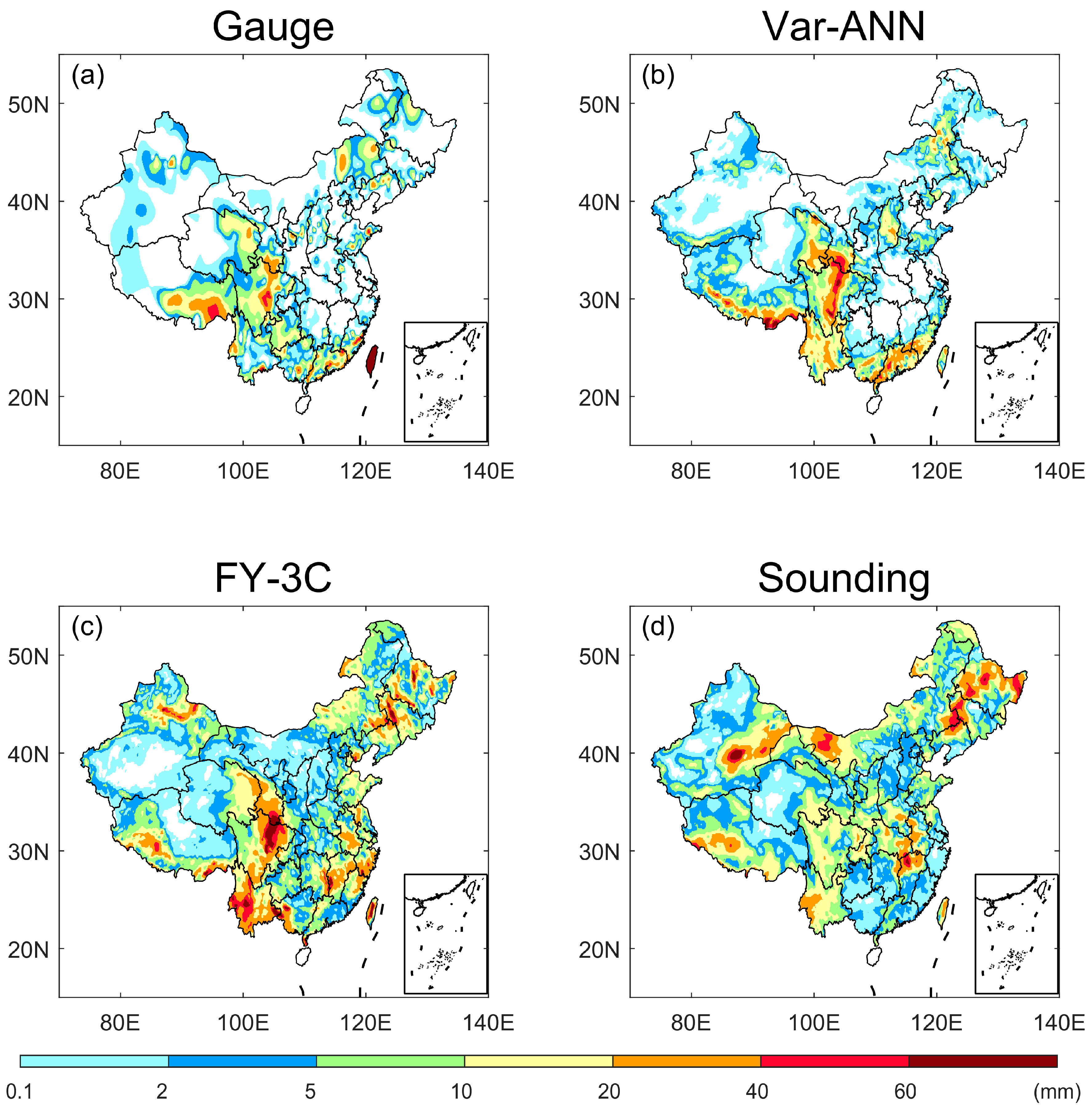
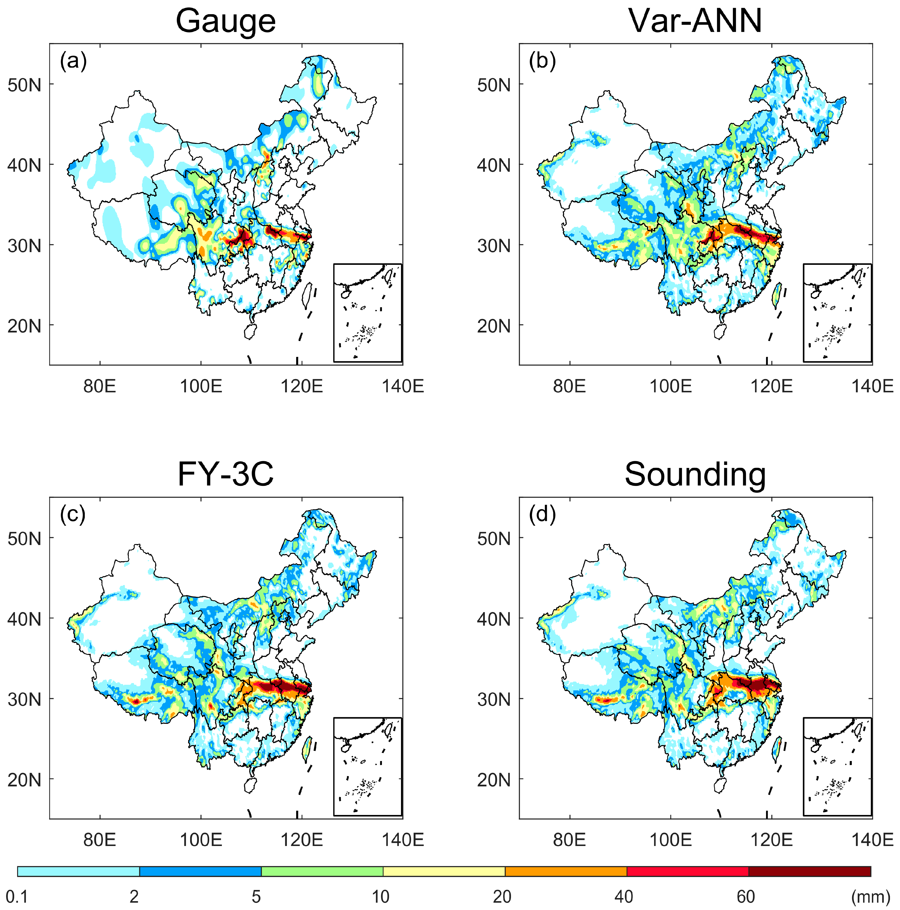
To further validate the accuracy of the calibrated data and its applicability in NWP data assimilation, the Weather Research and Forecast (WRF) Model was employed to simulate precipitation downstream of the TP. Two cases, specifically 12 July 2019 and 14 June 2020,were selected for WRF simulations. In these instances, convective cells that formed over the southeastern TP propagated eastward and generated heavy rainfall over the downstream region to the east of the TP. The selection criteria focus on their typical development process: TP-based convective initiation, westerly-affected eastward movement, upscale growth into organized convective systems, and resultant precipitation. A large number of previous studies have investigated this process, and their results indicate that the atmospheric conditions in the southeastern TP are highly correlated with convection and precipitation in the downstream regions [2,20,33]. If the calibrated data can effectively simulate this process, it will not only verify the accuracy of the data but also facilitate a deeper understanding of this process. To confirm the reliability of our dataset and reveal this mechanism, three distinct simulation schemes were designed. Two typical summer cases were selected for WRF simulation; the results are presented in Figure 6 and Figure 7. The “GFS” scheme uses the Global Forecast System (GFS) of the NCEP as the initial field, which is commonly employed in precipitation forecasting. The “FY3C” and “Sounding” schemes assimilate the original satellite and station data as the initial field, respectively, while the “Var-ANN” scheme assimilates the calibrated dataset developed in this study. The spatial distribution of gauge and simulated precipitation on 10 June 2019 is presented in Figure 6. It was found that the Sichuan Basin exhibits a pronounced precipitation center resulting from the aforementioned mechanism. Among the designed schemes, Var-ANN calibration alone accurately reproduced this case, whereas both the FY3C and Sounding schemes yielded inaccurate results. This inaccuracy is attributed to the insufficient accuracy of the FY3C atmospheric profiles and the sparse distribution of sounding stations.

To quantitatively analyze the errors associated with different data assimilation methods, several evaluation metrics for precipitation simulation results are presented in

Table 4. Two cases selected for daily evaluation: 12 July 2019 (Case 1) and 14 June 2020 (Case 2).

		GFS	FY3C	Sounding	FY-CLB
Case 1	RMSE	11.65	9.61	5.76	5.6
	Bias	7.94	3.33	−1.49	1.21
	TS	55.88	53.62	65.09	66.93
	FAR	44.16	44.19	30.8	35.82
Case 2	RMSE	9.18	14.08	6.59	6.46
	Bias	5.07	2.37	1.62	1.49
	TS	57.7	55.75	63.31	66.7
	FAR	48.09	49.64	41.57	38.79

Unit: mm for RMSE and Bias, % for TS, MR, and FAR. Bold font indicates the scheme with the best performance.

. Compared with the GFS scheme, the simulation accuracies of the other three schemes are improved, illustrating the role of data assimilation in simulation optimization. RMSE and bias reflect the overall errors across all samples; the FY-CLB scheme yields the lowest RMSE and bias, indicating its superior accuracy. TS and FAR are commonly used for spatial verification of precipitation. TS quantifies the fraction of observed precipitation events that were correctly predicted. It penalizes both false alarms and missed events, with 1 indicating perfect prediction. FAR denotes the false alarm rate. This metrics disregard precipitation intensity and only evaluate the accuracy of precipitation occurrence.

It is worth noting that in Case 1, the FAR of the FY-CLB scheme (35.82%) is slightly higher than that of the Sounding scheme (30.80%). This reflects a known trade-off between detection sensitivity and false alarm suppression; the Var-ANN calibration reduces the cold bias in VASS temperature profiles (Table 3), leading to warmer and more realistic lower-tropospheric initial conditions. This enhances convective available potential energy (CAPE) in the WRF model, resulting in more active precipitation prediction that captures additional true precipitation events (higher TS) but also generates a modest number of additional false alarms in marginal convective environments. In Case 2, FY-CLB achieves the lowest FAR (38.79% vs. 41.57% for Sounding), confirming that the overall performance is robust and the Case 1 FAR result is case-dependent rather than systematic. When all four metrics (RMSE, Bias, TS, FAR) are considered together, FY-CLB ranks first or second across all four, supporting its superior comprehensive performance.

We acknowledge that the WRF-based evaluation, while expanded to five cases (two in the main text and three additional in Supplementary S1), remains limited in scope. These five cases span different months (June, July, August), different years (2019, 2020), and different synoptic regimes (monsoon depression, Tibetan Plateau Vortex convection, and mei-yu frontal system). Nevertheless, they remain insufficient to establish statistically robust operational forecast improvements. The results presented here should be interpreted as a proof-of-concept demonstration. A comprehensive, multi-year, multi-season evaluation over a larger sample of precipitation events would be required to confirm the operational reliability of Var-ANN-calibrated profiles for NWP.

4. Conclusions and Discussion

Prior machine-learning-based satellite temperature calibration studies have typically relied on direct satellite–radiosonde collocation pairs for training, which are sparse over complex terrain. They have been trained on the original retrieval product without a physically constrained reference, or focused on global or mid-latitude regions without addressing the specific challenges of the Tibetan Plateau (e.g., strong surface heterogeneity, limited station density, and the systematic cold bias in infrared-based retrievals). In summary, the key distinctions of this work are (i) the use of variationally corrected station fields to construct a spatially consistent training dataset, mitigating the sparsity of direct collocation pairs over the western TP; (ii) the integration of cloud amount and geographic information as auxiliary predictors; and (iii) the targeted application to FY-3C VASS over the TP with WRF assimilation validation.

To provide accurate, high-resolution initial atmospheric field for NWP simulation over the TP, this study integrates the variation method and artificial neural network(Var-ANN) to calibrate satellite-derived temperature profiles, subsequently assimilating the calibrated data into the NWP model to simulate downstream precipitation. The background temperature field is derived from the Vertical Atmospheric Sounding System (VASS) product of the FY-3C satellite. As detailed in He et al. [34], this product is retrieved from MWHS, MWTS, and IRAS measurements using a multiple linear regression algorithm, which derives regression coefficients from prior atmospheric samples and converts brightness temperature into atmospheric temperature profiles. While this method enables rapid temperature profile retrieval, it cannot adequately account for nonlinear factors such as satellite zenith angle. To address this issue, the FY-3C retrieval algorithm partitions atmospheric samples into multiple subsets. Although these subsets can approximate nonlinear variations, they often struggle to preserve spatial homogeneity. Figure 3 reveals a pronounced high-value region, typically occurring at large satellite zenith angles, which is attributed to the retrieval scheme. In addition, uncertainties of cloud radiation simulation within RTM remain a critical issue, which further degrades the quality of the retrieved atmospheric profiles. To cope with these issues in this study, we additionally incorporate satellite zenith angle, geographic information, and cloud parameters as input features in the Var-ANN framework to better capture the radiative signals associated with atmospheric temperature. The ANN method has been widely applied in atmospheric data calibration; most studies use satellite-observed brightness temperatures as input training data and radiosonde observations as the target output [35,36,37]. A key advantage of the proposed Var-ANN configuration is that it treats radiosonde measurements as the most representative of real atmospheric conditions. Using variational analysis data as the training output not only significantly expands the training sample size but also enables the Var-ANN model to extract more accurate details of the atmospheric vertical structure.

The Var-ANN calibration results demonstrate that the framework effectively captures the dominant empirical relationships between satellite brightness temperatures and atmospheric temperature profiles as represented by radiosonde observations. As a result, the accuracy of the calibrated temperature profiles is substantially improved compared to the original VASS product, with an approximately 60% reduction in RMSE and a reduction in mean bias from approximately −5 °C to −0.7 °C. These improvements confirm the effectiveness of the variational-training-target approach for satellite temperature profile calibration over complex terrain.

Compared with prior satellite temperature profile retrieval and calibration studies over the Tibetan Plateau, the Var-ANN framework achieved a post-calibration RMSE of approximately 1.8–2.5 °C. This performance is comparable to that reported for neural-network-based retrieval and calibration methods applied over less challenging terrain. Given the complexity of the Tibetan Plateau, the limited density of training observations over the western TP, and the systematic cold bias inherent in the original VASS product, this level of accuracy represents meaningful progress. Notably, the RMSE reduction of approximately 60% relative to the original FY-3C VASS product (from 7.30 °C to 2.11 °C) is among the largest fractional improvements reported among satellite temperature calibration studies, reflecting the particular efficacy of the variationally constrained training dataset. In terms of downstream NWP impact, the threat scores of 66.9% (Case 1) and 66.7% (Case 2) obtained after assimilating Var-ANN-calibrated temperature profiles demonstrate that the improved thermal structure translates into measurable precipitation forecast skill over the TP. This is notable given that satellite data assimilation over the Tibetan Plateau has historically been challenging due to the complex terrain and sparse conventional observations, and few prior studies have quantitatively linked satellite temperature profile calibration to downstream precipitation forecast skill in this region. Across the five cases evaluated (two in the main text and three additional cases in Supplementary S1), the FY-CLB scheme consistently achieved the highest TS and CSI scores, with an average TS improvement of 12.7 percentage points over FY-ORG (65.2% vs. 52.5%). A paired t-test confirmed that this improvement is statistically significant at the p < 0.01 level, providing confidence that the Var-ANN calibration yields consistent gains across different synoptic regimes rather than being limited to favorably selected cases.

Specifically, He et al. [34] applied a shallow neural network for bias correction of FY-3C MWTS temperature retrievals over China and reported post-correction RMSE of ~2.0–3.0 K, though their approach relied on direct satellite–radiosonde collocation pairs without variational preprocessing. Zhang et al. [38] combined an artificial neural network with 1D-Var for FY-3D/HIRAS temperature retrieval over Europe, achieving an RMSE reduction of ~0.5 K relative to conventional bias correction, demonstrating the benefit of integrating physical constraints with statistical learning. Huang et al. [36] similarly integrated ANN with 1D-Var for FY-4A/GIIRS hyperspectral data over East Asia, reporting improved retrieval accuracy across multiple pressure levels. Hu et al. [35] applied deep neural networks to FY-3D/VASS temperature and humidity retrieval in the Arctic, achieving RMSE within ~4 K, and highlighted that machine learning methods are particularly advantageous in regions where complex surface conditions challenge physical retrieval algorithms—a conclusion that aligns with our experience over the Tibetan Plateau. Filei et al. [11] demonstrated neural network-based temperature retrieval from the Russian Meteor-M MTVZA-GY microwave radiometer, with comparable accuracy. Relative to these prior efforts, the present Var-ANN framework is distinguished by (i) the use of variationally corrected fields rather than raw satellite-radiosonde collocations as training targets, which provides spatially coherent supervision in data-sparse regions; (ii) optimization specifically for the Tibetan Plateau, where the combination of high altitude, strong surface heterogeneity, and systematic cold bias in IR-based retrievals presents unique challenges not addressed in prior regional studies; and (iii) quantitative evaluation of downstream WRF precipitation forecast skill across multiple synoptic regimes (Supplementary S1), extending beyond the retrieval accuracy metrics reported in most prior work.

To assess cross-seasonal generalizability, the Var-ANN model trained on summer (June–August) 2019 data was applied to an independent winter period (December 2019–January 2020). Performance degraded moderately in winter, with RMSE increasing from approximately 2.1 °C to approximately 3.5 °C in the mid-troposphere. This degradation is attributed to (a) different cloud regimes (predominantly ice clouds in winter versus deep convective clouds in summer), (b) stronger and more frequent surface temperature inversions over the TP in winter, and (c) reduced representativeness of the summer-dominated training sample for winter atmospheric conditions. Spatial consistency analysis reveals that calibration performance was best over the eastern and central TP (|bias| < 0.5 °C at 500 hPa) and somewhat reduced over the western and northern TP (|bias| up to 1.5 °C), consistent with the station density gradient (Figure 1). A temporal stability check across the summer months (June–August 2019) showed no systematic drift in monthly-mean bias or RMSE, with slightly larger errors in August associated with the peak of the Asian summer monsoon. Overfitting assessment using a 10% holdout validation set indicates an RMSE gap of less than 0.3 °C between training and validation sets, suggesting acceptable generalization with regard to the summer period. However, this does not guarantee generalization to other seasons or years, and these limitations are discussed further below.

High-resolution satellite data can provide NWP models with more detailed information regarding the thermal structure of the atmosphere over the TP. However, the accuracy of satellite-derived temperature profiles remains limited, particularly over complex terrain. The Var-ANN calibration framework presented here represents a practical step toward bridging the gap between satellite retrievals and the accuracy requirements of modern data assimilation systems.

The dynamic and thermal effects of the TP exert a substantial influence on the development of small-scale convection and the occurrence of precipitation over the region. During summer, the TP is characterized by abundant water vapor, which readily forms precipitation under the influence of vortices and shear lines over the TP. Local intense convection generated in this process propagates eastward under the steering of westerly winds, continuously incorporating additional water vapor and intensifying, ultimately leading to heavy precipitation events over the downstream middle and lower reaches. However, owing to the complex terrain of the TP, the spatial resolution of in situ observations remains limited, and even after calibration, satellite-derived temperature profiles retain uncertainties that propagate into downstream NWP simulations. The Var-ANN framework presented in this study offers a practical approach for improving the utility of FY-3C VASS temperature products for NWP over the TP, with the explicit understanding that further validation over larger samples and diverse meteorological conditions is needed to establish operational robustness.

References

1. Brown, A.; Davis, K. Uncertainty quantification in remote sensing temperature profiles. Atmos. Meas. Tech. 2021, 14, 4567–4582. [Google Scholar]
2. Zhang, S.; Xu, X.; Peng, S.; Yao, W.; Koike, T. Three-Dimensional Variational Data Assimilation Experiments for a Heavy Rainfall Case in the Downstream Yangtze River Valley Using Automatic Weather Station and Global Positioning System Data in Southeastern Tibetan Plateau. J. Meteorol. Soc. Jpn. 2014, 92, 483–500. [Google Scholar] [CrossRef] [Scilit]
3. Li, H.; Hu, Y.; Zhou, Z.; Peng, J.; Xu, X. Characteristic Features of the Evolution of a Meiyu Frontal Rainstorm with Doppler Radar Data Assimilation. Adv. Meteorol. 2018, 2018, 9802360. [Google Scholar] [CrossRef] [Scilit]
4. Li, H.; Xu, X.; Hu, Y.; Xiao, Y.; Wang, Z. Assimilation of Doppler Radar Data and Its Impact on Prediction of a Heavy Meiyu Frontal Rainfall Event. Adv. Meteorol. 2018, 2018, 9482014. [Google Scholar] [CrossRef] [Scilit]
5. Lu, Q.; Yang, X.; Wu, C.; Zheng, J.; Qin, D.; Yang, H.; Zhang, P. An Initial Study on Assimilating Satellite-derived Total Precipitable Water in a Variational Assimilation System. In Proceedings of the Progress in Electromagnetics Research Symposium, Suzhou, China, 12–16 September 2011. [Google Scholar]
6. Maggioni, V.; Reichle, R.H.; Anagnostou, E.N. The Efficiency of Assimilating Satellite Soil Moisture Retrievals in a Land Data Assimilation System Using Different Rainfall Error Models. J. Hydrometeorol. 2013, 14, 368–374. [Google Scholar] [CrossRef] [Scilit]
7. Raju, A.; Parekh, A.; Sreenivas, P.; Chowdary, J.S.; Gnanaseelan, C. Estimation of Improvement in Indian Summer Monsoon Circulation by Assimilation of Satellite Retrieved Temperature Profiles in WRF Model. IEEE J. Sel. Top. Appl. Earth Obs. Remote Sens. 2015, 8, 1591–1600. [Google Scholar] [CrossRef] [Scilit]
8. Eyre, J.R.; English, S.J.; Forsythe, M. Assimilation of satellite data in numerical weather prediction. Q. J. R. Meteorol. Soc. 2020, 146, 49–68. [Google Scholar] [CrossRef] [Scilit]
9. Lian, X.; Zeng, Z.; Yao, Y.; Peng, S.; Wang, K.; Piao, S. Spatiotemporal variations in the difference between satellite-observed daily maximum land surface temperature and station-based daily maximum near-surface air temperature. J. Geophys. Res. Atmos. 2017, 122, 2254–2268. [Google Scholar] [CrossRef] [Scilit]
10. Esmaili, R.; Smith, N.; Schoeberl, M.; Barnet, C. Evaluating Satellite Sounding Temperature Observations for Cold Air Aloft Detection. Atmosphere 2020, 11, 1360. [Google Scholar] [CrossRef] [Scilit]
11. Filei, A.A.; Andreev, A.I.; Uspensky, A.B. Using of a Neural Network Algorithm for Retrieval Temperature and Humidity Sounding of the Atmosphere from Satellite-Based Microwave Radiometer MTVZA-GY Measurements On-Board Meteor-M No. 2-2. Issled. Zemli Kosmosa 2021, 83-95, 1515–1526. [Google Scholar]
12. Orlandi, E.; Fierli, F.; Davolio, S.; Buzzi, A.; Drofa, O. A nudging scheme to assimilate satellite brightness temperature in a meteorological model: Impact on representation of African mesoscale convective systems. Q. J. R. Meteorol. Soc. 2010, 136, 462–474. [Google Scholar] [CrossRef] [Scilit]
13. Shi, X.; Li, Y.; Liu, J.; Xiang, X.; Liu, L. Simulation of FY-2D infrared brightness temperature and sensitivity analysis to the errors of WRF simulated cloud variables. Sci. China-Earth Sci. 2018, 61, 957–972. [Google Scholar] [CrossRef] [Scilit]
14. Wang, K.C.; Dickinson, R.E.; Wild, M.; Liang, S. Atmospheric impacts on climatic variability of surface incident solar radiation. Atmos. Chem. Phys. 2012, 12, 9581–9592. [Google Scholar] [CrossRef] [Scilit]
15. Hu, L.; Deng, D.; Gao, S.; Xu, X. The seasonal variation of Tibetan Convective Systems: Satellite observation. J. Geophys. Res. Atmos. 2016, 121, 5512–5525. [Google Scholar] [CrossRef] [Scilit]
16. Zhang, Y.; Zhao, L.; Wang, W.; Tang, S.; Huang, F. Summer ozone variation derived from FY3/TOU satellite data and impacts of East Asian summer monsoon. In Proceedings of the Remote Sensing of the Atmosphere, Clouds, and Precipitation VII, Honolulu, HI, USA, 24–26 September 2018. [Google Scholar]
17. Herman, B.M.; Brunke, M.A.; Pielke, R.A., Sr.; Christy, J.R.; McNider, R.T. Satellite Global and Hemispheric Lower Tropospheric Temperature Annual Temperature Cycle. Remote Sens. 2010, 2, 2561–2570. [Google Scholar] [CrossRef] [Scilit]
18. He, J.; Zhang, S.; Wang, Z. The retrievals and analysis of clear-sky water vapor density in the Arctic regions from MWHS measurements on FY-3A satellite. Radio Sci. 2012, 47, RS2009. [Google Scholar] [CrossRef] [Scilit]
19. Guo, L.; An, N.; Wang, K.C. Reconciling the discrepancy in ground- and satellite-observed trends in the spring phenology of winter wheat in China from 1993 to 2008. J. Geophys. Res. Atmos. 2016, 121, 1027–1042. [Google Scholar] [CrossRef] [Scilit]
20. Chen, B.; Xu, X.D.; Yang, S.; Bian, J.C. On the characteristics of water vapor transport from atmosphere boundary layer to stratosphere over Tibetan Plateau regions in summer. Chin. J. Geophys. Chin. Ed. 2012, 55, 406–414. [Google Scholar]
21. Li, Q.; Zhao, R.; Sun, M. A hybrid approach for satellite data calibration based on variation analysis. J. Atmos. Ocean. Technol. 2024, 41, 89–102. [Google Scholar]
22. Chen, S.H.; Sun, W.Y. A one-dimensional time dependent cloud model. J. Meteorol. Soc. Jpn. 2002, 80, 99–118. [Google Scholar] [CrossRef] [Scilit]
23. Kain, J.S. The Kain–Fritsch convective parameterization: An update. J. Appl. Meteorol. 2004, 43, 170–181. [Google Scholar] [CrossRef] [PubMed]
24. Dudhia, J. Numerical study of convection observed during the Winter Monsoon Experiment using a mesoscale two-dimensional model. J. Atmos. Sci. 1989, 46, 3077–3107. [Google Scholar] [CrossRef]
25. Mlawer, E.J.; Taubman, S.J.; Brown, P.D.; Iacono, M.J.; Clough, S.A. Radiative transfer for inhomogeneous atmospheres: RRTM, a validated correlated-k model for the longwave. J. Geophys. Res. 1997, 102, 16663–16682. [Google Scholar] [CrossRef] [Scilit]
26. Smith, J.; Wang, L. Satellite temperature retrieval using deep neural networks. Remote Sens. 2023, 15, 1123–1138. [Google Scholar] [CrossRef] [Scilit]
27. Norris, J.R.; Wild, M. Trends in aerosol radiative effects over China and Japan inferred from observed cloud cover, solar “dimming,” and solar “brightening”. J. Geophys. Res. 2009, 114, D00D15. [Google Scholar] [CrossRef] [Scilit]
28. Xie, X.; Wu, S.; Xu, H.; Yu, W.; He, J.; Gu, S. Ascending–Descending Bias Correction of Microwave Radiation Imager on Board FengYun-3C. IEEE Trans. Geosci. Remote Sens. 2019, 57, 3126–3134. [Google Scholar] [CrossRef]
29. Mason, B.J. The role of clouds in the radiative balance of the atmosphere and their effects on climate. Contemp. Phys. 2002, 43, 1–11. [Google Scholar] [CrossRef] [Scilit]
30. Xu, X.; Zhao, T.; Lu, C.; Guo, Y.; Chen, B.; Liu, R.; Li, Y.; Shi, X. An important mechanism sustaining the atmospheric "water tower" over the Tibetan Plateau. Atmos. Chem. Phys. 2014, 14, 11287–11295. [Google Scholar] [CrossRef] [Scilit]
31. Zhao, Y.; Xu, X.; Chen, B.; Wang, Y. The upstream "strong signals" of the water vapor transport over the Tibetan Plateau during a heavy rainfall event in the Yangtze River Basin. Adv. Atmos. Sci. 2016, 33, 1343–1350. [Google Scholar] [CrossRef] [Scilit]
32. Yang, S.; Zhang, W.; Chen, B.; Xu, X.; Zhao, R. Remote moisture sources for 6-hour summer precipitation over the Southeastern Tibetan Plateau and its effects on precipitation intensity. Atmos. Res. 2020, 236, 104803. [Google Scholar] [CrossRef] [Scilit]
33. Wang, Y.; Xu, X.; Lupo, A.R.; Li, P.; Yin, Z. The remote effect of the Tibetan Plateau on downstream flow in early summer. J. Geophys. Res. 2011, 116, D19110. [Google Scholar] [CrossRef] [Scilit]
34. He, J.; Wang, Z.; He, Q. Bias Correction for Retrieval of Atmospheric Parameters from the Microwave Humidity and Temperature Sounder Onboard the Fengyun-3C Satellite. Atmosphere 2016, 7, 156. [Google Scholar] [CrossRef] [Scilit]
35. Hu, J.; Wu, J.; Petropoulos, G.P.; Bao, Y.; Liu, J.; Lu, Q.; Wang, F.; Zhang, H.; Liu, H. Temperature and Relative Humidity Profile Retrieval from Fengyun-3D/VASS in the Arctic Region Using Neural Networks. Remote Sens. 2023, 15, 1648. [Google Scholar] [CrossRef] [Scilit]
36. Huang, P.; Guo, Q.; Han, C.; Zhang, C.; Yang, T.; Huang, S. An Improved Method Combining ANN and 1D-Var for the Retrieval of Atmospheric Temperature Profiles from FY-4A/GIIRS Hyperspectral Data. Remote Sens. 2021, 13, 481. [Google Scholar] [CrossRef] [Scilit]
37. Zhang, Y.; Chen, X.; Liu, H. Bias correction methods for atmospheric profile products. IEEE Trans. Geosci. Remote Sens. 2022, 60, 1–14. [Google Scholar]
38. Zhang, C.; Gu, M.; Hu, Y.; Huang, P.; Yang, T.; Huang, S.; Yang, C.; Shao, C. A Study on the Retrieval of Temperature and Humidity Profiles Based on FY-3D/HIRAS Infrared Hyperspectral Data. Remote Sens. 2021, 13, 2157. [Google Scholar] [CrossRef] [Scilit]
Figure 1. Distribution of sounding and meteorological stations. Black dots denote sounding stations, solid blue dots represent meteorological stations, and the colored background indicates geopotential height in meters.
Remotesensing 18 02746 g001
Figure 2. Comparison between satellite-derived temperature and radiosonde temperature. (a) Line-and-shading plot of vertical profiles of mean temperature from radiosonde observations (black solid line), raw VASS retrievals (red dashed line), and Var-ANN calibrated retrievals (blue solid line). Shaded areas denote ±1 standard deviation of the raw (red) and calibrated (blue) data. (b) Scatter density plot of raw VASS temperature versus radiosonde-observed temperature. (c) Scatter density plot of Var-ANN calibrated temperature versus radiosonde-observed temperature. The diagonal dashed line in (b,c) indicates the 1:1 agreement. Color shading represents point density.
Remotesensing 18 02746 g002
Figure 3. Spatial distribution of raw and calibrated temperature at 520 hPa. (a,b) show the original 25 km resolution, while (c,d) display the resampled products used to fill pixel gaps. The color bar represents atmospheric temperature in Celsius (°C).The red circles mark the areas where the improvements after revision are more obvious.
Remotesensing 18 02746 g003
Figure 4. Training process of the Var-ANN. (a) The performance and gradient of the machine learning model, with the blue axis and line representing the performance (mean squared error) and the orange axis and line denoting the gradient; (b) the constraint boundaries during training, with the blue axis and line corresponding to the number of validation failures and the orange axis and line representing the iterative parameter MU; (c,d) show comparisons for the training and testing datasets, respectively. The x-axis represents the radiosonde profiles used for training and testing, and the y-axis represents the corresponding model outputs. The red circles in (a) show the epochs at which training stopped because the conditions were satisfied. The red diamonds in (c) denote the epochs during which the validation increased.
Remotesensing 18 02746 g004
Figure 5. Correlation between input and output data in the machine learning model. The x-axis represents the input data, which includes geographical information, cloud parameters, and brightness temperature channels. The y-axis denotes the pressure levels of the raw data, which are determined by the radiative transfer model. The color gradient indicates the correlation coefficient between the input and output variables, while the markers (*) signify that the corresponding correlation coefficients are statistically significant at the 95% confidence level.
Remotesensing 18 02746 g005
Figure 6. Daily precipitation on 10 June 2019. (a) gauge precipitation, (b) calibrated data simulation, (c) FY3D-VASS original data simulation, and (d) sounding profile simulation.
Remotesensing 18 02746 g006
Figure 7. Daily precipitation on 14 July 2020. (a) gauge precipitation, (b) calibrated data simulation, (c) FY3D-VASS original data simulation, and (d) sounding profile simulation.
Remotesensing 18 02746 g007