Article

ACBDT: SAR-Optical Cross-Modal Distillation for Sentinel-1/2 Building-Footprint Mapping in Heterogeneous Yangtze River Delta Cities

1
School of Remote Sensing and Information Engineering, Wuhan University, Wuhan 430079, China
2
Hubei Luojia Laboratory, Wuhan 430079, China
3
Survey and Monitoring Institute of Hydrogeology and Environmental Geology of Hunan Province, Changsha 410129, China
*
Author to whom correspondence should be addressed.
Remote Sens. 2026, 18(17), 2868; https://doi.org/10.3390/rs18172868
Submission received: 28 June 2026 / Revised: 16 August 2026 / Accepted: 19 August 2026 / Published: 24 August 2026

Abstract

Medium-resolution building-footprint mapping is limited by two coupled problems: 10 m optical pixels mix roofs with roads and bare surfaces, and SAR observations are degraded by speckle and viewing geometry. We present ACBDT, a Sentinel-1/2 framework that encodes each modality separately, learns a diffusion-inspired time-step-conditioned fused teacher representation, transforms it through a Cross-Modal Distillation Bridge (CMDB), and refines the output with a Student Refinement Decoder. The time-step variable is used only as a stochastic conditioning index; ACBDT does not implement a forward noising schedule, reverse diffusion, or iterative diffusion sampling. Training and evaluation used 2680 paired 256 × 256 patches over eight Yangtze River Delta cities with a spatially disjoint block partition. In three independent runs on the held-out test partition, ACBDT achieved 85.61 ± 0.32% building IoU, 92.24 ± 0.19% F1, and 83.74 ± 0.34% dataset-level boundary F1, compared with 83.21 ± 0.24% IoU for the strongest baseline, FTransUNet. Repeated-seed ablation showed 79.01 ± 0.42% IoU without CMDB and 84.53 ± 0.20% IoU without time-step conditioning. The separate density diagnostic retained a positive full-minus-optical IoU difference across all five building-density strata. Conclusions are limited to this Yangtze River Delta evaluation; city-held-out and cross-season transfer were not tested.

1. Introduction

Accurate building-footprint maps are a prerequisite for estimating urban exposure, monitoring built-up expansion, and supporting disaster-risk and sustainability assessments. The Yangtze River Delta (YRD) is a demanding test region because rapid urban growth has produced dense megacity cores, peri-urban industrial belts, coastal settlements, and terrain-affected urban margins within a single economic region. Freely available Sentinel-1 SAR and Sentinel-2 optical data provide the spatial coverage and revisit frequency needed for such mapping, but the 10 m observation scale remains challenging where buildings are small, spectrally mixed, or shadowed by neighboring structures [1,2,3].
Single-sensor mapping cannot fully resolve this problem. Sentinel-2 supplies spectral and index information that separates vegetation, water, bare soil, and many impervious surfaces, yet it remains vulnerable to cloud, shadow, and roof-road confusion. Sentinel-1 adds all-weather backscatter, coherence, and dual-polarization structural cues related to scattering stability and urban geometry, but SAR-only interpretation is limited by speckle, layover, shadowing, and weak semantic discrimination. These physical differences make simple band stacking insufficient: fusion must preserve modality-specific evidence while controlling the conflicts introduced by different sensing geometries [4,5,6,7,8].
Multi-modal remote-sensing fusion has therefore shifted from pixel-, feature-, and decision-level combinations toward networks that learn when each modality should be trusted. Prior Sentinel-1/Sentinel-2 studies show that SAR-optical fusion can reduce confusion between built-up surfaces and spectrally similar land covers, especially when optical indices such as NDVI, NDWI, and NDBI are combined with structural SAR responses. The remaining challenge is not whether the two sensors are complementary, but how to align their features without forcing noisy SAR responses and optical semantics into a premature common representation [9,10,11,12,13].
Studies targeting SAR-optical built-up mapping sharpen this point. Sentinel-1/Sentinel-2 fusion has been shown to improve global urban extraction, and the residual difficulty lies less in sensor complementarity than in the domain shift encountered when a model trained in one urban context is applied to another [14]. Recent cross-fusion architectures for built-up extraction likewise report that gains depend on how modality-specific features are combined and on robustness to label noise, rather than on the addition of radar channels alone [15]. Related cross-modal work reaches the same conclusion from a representation-learning direction, whether by learning shared SAR-optical embeddings for land-cover labeling [16], by exploiting cross-layer interaction and multiscale fusion for high-resolution segmentation [17], or by recovering fine-grained structure from Sentinel-2 alone [18]. Sentinel-1 backscatter and dual-polarimetric descriptors have been used to map built-up areas directly, establishing that radar carries genuine structural information about the built environment while remaining weaker than optical data in semantic discrimination [19]. These results converge on a single design question: where in the network the two modalities should be aligned. ACBDT answers that question by deferring alignment until each branch has produced a stable representation, and then performing it in a dedicated bridge.
Deep segmentation models have improved remote-sensing mapping through encoder–decoder structures, attention mechanisms, and Transformer-based fusion. Even so, four issues remain central for Sentinel-scale building extraction: heterogeneous SAR-optical features must be aligned without erasing modality-specific evidence; building edges must be represented despite mixed pixels; performance must remain stable across heterogeneous urban morphology; and the deployed forward graph must remain tractable for wall-to-wall mapping. These requirements motivate an asymmetric teacher–student design rather than a purely symmetric fusion network [20,21,22,23,24,25,26,27,28,29,30].
Knowledge distillation and diffusion-inspired time-step conditioning enter this design for specific reasons rather than as generic additions. Cross-modal knowledge transfer has been applied in remote-sensing segmentation to move structured representations from a modality-rich teacher into a more constrained student, and multiscale variants report that the transfer is most effective when it operates on intermediate features rather than on outputs alone [31,32]. Diffusion models motivate the use of sinusoidal time embeddings as a general conditioning mechanism [33,34]; however, ACBDT does not implement a forward noising process or a learned reverse diffusion process. Instead, a randomly sampled time-step index is embedded and injected into teacher features as stochastic conditioning, while distillation transfers the teacher’s fused SAR-optical representation toward the decoder. Section 4.5.2 evaluates both CMDB and the time-step conditioning through controlled repeated-seed ablations [35,36,37,38,39].
Against this background, the present study proposes ACBDT for building-footprint extraction from Sentinel-1/2 data. The acronym is retained for continuity with the original submission, but the revised manuscript explicitly defines the D component as diffusion-inspired time-step conditioning rather than a generative diffusion model. The remote-sensing contribution is a test of whether SAR-optical complementarity can be made usable at Sentinel scale. The framework combines SAR-derived structural channels, Sentinel-2 multispectral bands, and NDVI, NDWI, and NDBI. CMDB is treated as the central cross-modal alignment mechanism, while the time-step-conditioned ATG and HAMSF form the teacher-side representation pathway [40,41,42,43,44].
First, the Cross-Modal Distillation Bridge (CMDB) implements the asymmetric teacher–student link by converting high-capacity SAR-optical teacher features into compact student features while preserving cross-modal alignment.
Second, the Hybrid Attention Multi-Scale Fusion (HAMSF) module introduces a multi-scale attention pathway inside the teacher to accommodate roof-size and contextual variation. Its isolated contribution is not treated as a principal claim in the present revision because the key robustness analysis focuses on CMDB and time-step conditioning.
Third, the Adaptive Teacher Generator (ATG) incorporates diffusion-inspired time-step conditioning as a training-time stochastic conditioning mechanism before the fused representation is transformed by CMDB and decoded by SRD. This component is not described as a diffusion generative process; its contribution is evaluated directly by removing all time-embedding injections in the controlled ablation of Section 4.5.2.
The design is intended to reduce modality conflict and improve boundary-sensitive extraction in spectrally ambiguous urban scenes. Its effectiveness is evaluated through a same-protocol benchmark, repeated-seed robustness and key-ablation analysis, and a separate density diagnostic reported in Section 4.
The study therefore tests whether asymmetric cross-modal feature transformation improves Sentinel-scale building mapping under roof-road confusion, mixed pixels, SAR speckle, and complex viewing geometry. The principal evidence consists of a controlled within-study benchmark against eight representative baselines, complemented by modality, bridge, density, error-structure, and implementation diagnostics. Spatial transfer beyond the internal YRD partition is treated as a limitation and reserved for dedicated held-out-city validation.
The remainder of the paper is organized as follows: Section 2 describes the study area, satellite data, preprocessing, and reference data. Section 3 presents the ACBDT methodology. Section 4 reports the results and diagnostic analyses. Section 5 discusses the physical interpretation, limitations, and future validation requirements. Section 6 concludes the study.

2. Study Area and Dataset

2.1. Study Area Description

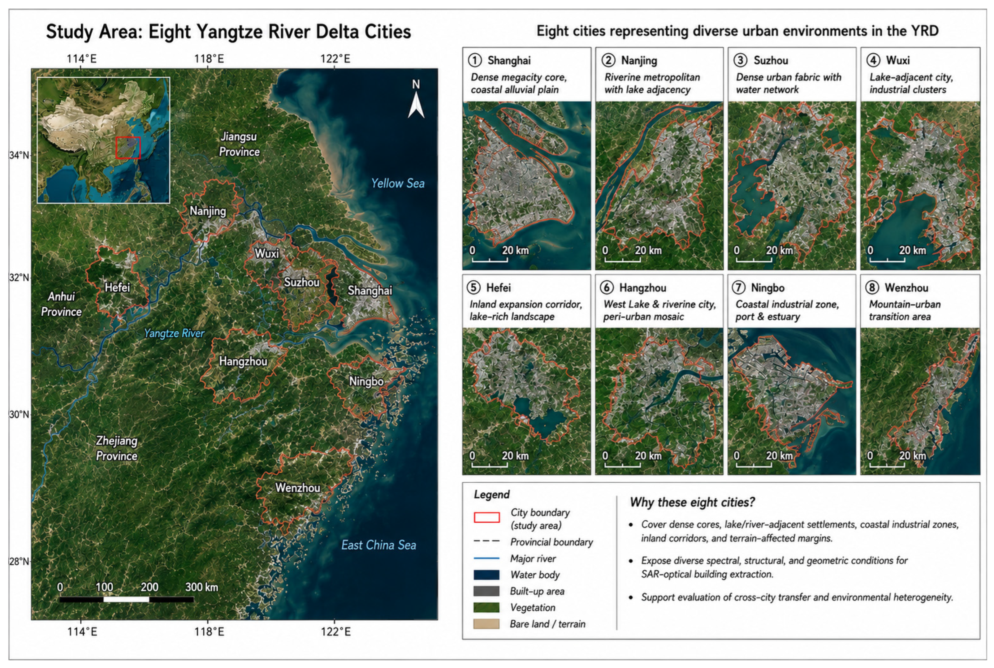
The study area covers eight cities in the Yangtze River Delta (YRD): Shanghai, Nanjing, Suzhou, Wuxi, Hefei, Hangzhou, Wenzhou, and Ningbo (Figure 1). The selection was not made simply for spatial coverage. These cities jointly represent dense metropolitan cores, lake- and river-adjacent settlements, coastal industrial zones, inland expansion corridors, and mountain-urban transition areas, giving the model a wide range of spectral, structural, and geometric conditions to resolve [1,2,3].
This design creates three useful sources of variation for evaluating building extraction. Shanghai and Suzhou test performance in dense urban fabrics with frequent shadows and narrow gaps; Hefei, Hangzhou, and Wuxi introduce mixed residential, industrial, and water-adjacent landscapes; Ningbo and Wenzhou add coastal and terrain-affected conditions where SAR geometry and optical texture can disagree. The YRD has also experienced rapid built-up expansion, so the region is relevant not only as a segmentation benchmark but also as an operational monitoring case.
Figure 1. Study-area configuration for the eight Yangtze River Delta cities.
Remotesensing 18 02868 g001
Figure 1 is used to anchor the sampling logic behind the experiments. The selected cities expose ACBDT to dense central districts, fragmented peri-urban settlements, extensive water boundaries, and locally complex terrain. This spatial diversity matters because the same building class can appear as bright roof spectra in the optical image, high double-bounce response in SAR, weak backscatter in small residential blocks, or distorted geometry in layover-prone terrain. The dataset is therefore a demanding internal test of SAR-optical complementarity rather than a narrow single-city case [4,5,24,45].

2.2. Satellite Data and Preprocessing

2.2.1. Sentinel-1 SAR Data

C-band Sentinel-1 SAR imagery acquired in Interferometric Wide (IW) swath mode was used [4]. All products are Sentinel-1A; no Sentinel-1B product is included because Sentinel-1B ceased radar acquisition in December 2021 and its mission was formally ended in 2022. The dataset comprises 231 dual-polarization Single Look Complex products (product type IW SLC, polarization mode 1SDV, VV/VH) acquired between 2 June and 30 September 2024 over the eight study cities on relative orbits 69, 142, and 171. Table 1 summarizes the acquisition inventory by city, orbit, date range, and coherence-pair count.
Table 1. City-level summary of the Sentinel-1A and Sentinel-2 products used in this study.
CitySentinel-1A IW SLC ProductsRelative Orbit(s)Sentinel-1 Date Range (2024)Coherence PairsSentinel-2 L2A ProductsSentinel-2 Date Range (2024)
Hangzhou10697 June–23 September9501 June–29 September
Hefei2014212 June–28 September92032 June–30 September
Nanjing4069, 1427 June–28 September18521 June–29 September
Ningbo4269, 1712 June–30 September19981 June–29 September
Shanghai201712 June–30 September10491 June–29 September
Suzhou4069, 1712 June–30 September191001 June–29 September
Wenzhou3169, 1712 June–30 September191971 June–29 September
Wuxi2869, 1712 June–30 September151001 June–29 September
Total23169, 142, 1712 June–30 September1188491 June–30 September
Interferometric coherence was computed from 118 repeat-pass SLC pairs. Pairs were formed under three constraints: identical pass direction, identical relative orbit, and a nominal 12-day temporal baseline, the shortest repeat interval available from the single-satellite Sentinel-1A constellation during the acquisition window. Holding pass and orbit constant keeps the perpendicular baseline small and the viewing geometry fixed, so that coherence loss is dominated by temporal decorrelation and scattering stability rather than by geometric decorrelation [7]. This matters for building extraction because rigid built structures retain high coherence over 12 days whereas vegetation decorrelates rapidly, a contrast that has been exploited both for global building mapping from Sentinel-1 and for coherence-based land-cover classification [46,47]. Processing followed the standard interferometric chain: precise-orbit application, split and deburst of the relevant IW sub-swaths, coregistration to sub-pixel accuracy using the Copernicus GLO-30 digital elevation model with enhanced spectral diversity refinement, interferogram formation, and coherence estimation in a 5 × 5 pixel moving window. Multilooking used 4 range looks and 1 azimuth look, producing approximately square ground pixels that were terrain-corrected and resampled to a common 10 m grid. Speckle reduction used a refined Lee 5 × 5 filter applied to the backscatter channels only; coherence was not speckle-filtered because the estimation window already averages spatially [6].
Backscatter products were calibrated to sigma-nought, terrain-corrected using the same elevation model, and converted to decibels. Where multiple acquisitions covered a city, the backscatter channels were temporally averaged over the June–September window to suppress residual speckle and transient surface change, while the coherence channels were averaged over the available 12-day pairs for that city.
The SAR branch supplies seven channels. Table 2 lists each channel with its definition and physical role. VV_dB and VH_dB are calibrated backscatter coefficients in decibels, VV_dB = 10 log10(sigma0_VV) and VH_dB = 10 log10(sigma0_VH). VV_Coh and VH_Coh are the interferometric coherence magnitudes of the co-polarized and cross-polarized 12-day pairs. The remaining three channels are structural descriptors derived from the dual-polarization covariance matrix C2, estimated over a 5 × 5 window from the VV and VH complex scattering amplitudes. Writing the eigenvalues of C2 as lambda_1 >= lambda_2 and the normalized eigenvalue probabilities as p_i = lambda_i/(lambda_1 + lambda_2 + epsilon) with epsilon = 1 × 10⁻¹⁵, the three descriptors are the entropy-like parameter H = −sum_i p_i log2(p_i), the alpha-like parameter Alpha = sum_i p_i alpha_i where alpha_i is the scattering angle extracted from the corresponding eigenvector of C2, and the polarimetric-difference parameter Pd = (lambda_1 − lambda_2)/(lambda_1 + lambda_2 + epsilon).
Table 2. Definition and physical interpretation of the seven Sentinel-1 derived input channels.
#ChannelDefinitionPhysical Role
1VV_dB10 log10(sigma0_VV), terrain-corrected, temporally averagedCo-polarized backscatter; strong double-bounce from building-ground dihedrals
2VH_dB10 log10(sigma0_VH), terrain-corrected, temporally averagedCross-polarized backscatter; sensitive to volume scattering and depolarizing targets
3VV_CohInterferometric coherence magnitude, VV, 12-day pair, 5 × 5 windowTemporal stability of co-polarized scattering; high over rigid built structures
4VH_CohInterferometric coherence magnitude, VH, 12-day pair, 5 × 5 windowTemporal stability of cross-polarized scattering; low over vegetation
5H-sum_i p_i log2(p_i), p_i = lambda_i/(lambda_1 + lambda_2 + eps), C2 over 5 × 5, eps = 1 × 10⁻¹⁵Entropy-like scattering randomness (dual-pol approximation, bounded by 1)
6Alphasum_i p_i alpha_i, alpha_i from the C2 eigenvectorsAlpha-like mean scattering angle; separates surface, dipole, and dihedral regimes (dual-pol approximation)
7Pd(lambda_1 − lambda_2)/(lambda_1 + lambda_2 + eps)Normalized eigenvalue contrast; dominance of a single scattering mechanism (anisotropy analog)
An important qualification applies to H, Alpha, and Pd. Sentinel-1 IW data are dual-polarization rather than quad-polarization, so the 2 × 2 covariance matrix does not span the full scattering space, and these quantities are not the canonical Cloude-Pottier entropy, mean alpha angle, and anisotropy defined for coherency matrices [8]. The consequences are specific and bounded: H is bounded by log2(2) = 1 rather than log2(3), Alpha is derived from a two-dimensional eigenvector basis, and Pd is a normalized eigenvalue contrast that plays a role analogous to but not identical to full-polarimetric anisotropy. Dual-polarimetric adaptations of the Cloude-Pottier decomposition are established in the literature and are explicitly formulated as modified, partial decompositions [48], and comparative work confirms that dual-polarimetric descriptors lose discriminative information relative to quad-polarimetric data [49]. The descriptors are therefore used here as reproducible measures of scattering randomness and dominance, informative for separating the stable structured response of built surfaces from the more random volume scattering of vegetation, and they are labeled dual-polarization approximations throughout rather than as full-polarimetric parameters. The SAR-derived layers provide structural and dielectric information that complements the optical branch, while the interpretation remains bounded by the dual-polarization nature of Sentinel-1 IW data [4,8].

2.2.2. Sentinel-2 Optical Data

Sentinel-2A and Sentinel-2B MultiSpectral Instrument (MSI) Level-2A surface-reflectance products were used as the optical source [5,50]. The inventory comprises 849 Level-2A products (430 Sentinel-2A and 419 Sentinel-2B) acquired between 1 June and 30 September 2024 over the study cities. Cloud and shadow screening was performed during preprocessing using the Level-2A scene classification information, and each Sentinel-1 acquisition was associated with the temporally nearest qualifying Sentinel-2 observation. Table 1 provides the city-level optical acquisition inventory.
Sentinel-2 preprocessing used Level-2A surface reflectance as the optical basis. Cloud and shadow pixels were removed using the Scene Classification Layer, 20 m bands were resampled to 10 m by bilinear interpolation, and reflectance values were clipped and scaled to a common numeric range. This processing produced a summer composite that is spatially aligned with the SAR stack and suitable for patch-based fusion [50,51,52].
The optical branch contains five reflectance bands (Blue B2, Green B3, Red B4, NIR B8, and SWIR1 B11) and three indices selected for land-cover separation. NDVI emphasizes vegetation, NDWI identifies water bodies, and NDBI enhances built-up surfaces relative to vegetation. These channels provide the semantic contrast that SAR alone lacks, while the SAR branch contributes structural evidence where optical spectra are ambiguous [40,41,42]. These eight optical features supply complementary spectral information on vegetation, water, and impervious surfaces, serving as the optical branch input.

2.2.3. Multi-Modal Data Co-Registration

Pixel-level fusion requires that SAR and optical observations refer to the same ground locations. Both datasets were projected to UTM Zone 51N (WGS84), resampled to 10 m, and fine-aligned using stable control features such as road intersections and bridges. Sub-pixel alignment was checked with cross-correlation, normalized mutual information, and visual inspection, reducing the risk that apparent model errors are caused by preprocessing displacement rather than segmentation failure [9,10,53].
The final multi-modal stack comprises the implemented SAR-derived structural channels and eight optical channels, tiled into non-overlapping 256 × 256 pixel patches (corresponding to 2.56 km × 2.56 km on the ground). The same channel configuration is used consistently for training, validation, and wall-to-wall inference.

2.3. Reference Data Preparation

Reference masks were constructed from OpenStreetMap building polygons and then manually corrected against high-resolution Google Earth imagery. Where official cadastral data were available, they were used as an additional consistency check. This multi-source procedure improves label completeness relative to raw OSM alone, but it also means that the reference set should be regarded as an internally curated product rather than an independently published benchmark [53,54].
Binary raster masks were generated at 10 m resolution (0 = background, 1 = building) by rasterizing the corrected polygons with an all-touched rule, so that any cell intersected by a footprint is labeled as building. No morphological dilation was applied to the reference masks used for the reported results. At 10 m ground sampling, a one-pixel dilation changes the footprint geometry by 10 m and can materially alter recall and boundary agreement; all benchmark and diagnostic evaluations therefore use the same undilated mask definition.
The final eight-city dataset contains 2680 non-overlapping 256 × 256 patches. Partitions were assigned by contiguous spatial blocks rather than by independent random sampling: 2144 patches (80%) form the training partition, 268 patches (10%) form the validation partition used for checkpoint selection and hyperparameter choice, and 268 patches (10%) form a held-out test partition used for neither model fitting nor checkpoint selection. Block assignment is a deliberate design choice rather than a convenience. Randomly split geospatial samples are spatially autocorrelated, and neighboring patches placed on opposite sides of a split share morphology, acquisition geometry, and annotation style, which can inflate reported accuracy relative to genuinely new ground [55,56]. The held-out 268-tile test partition is used for the broad same-protocol reference benchmark and for the repeated-seed robustness and key-ablation analysis. A separate 416-tile recovered-checkpoint record is retained only for the density diagnostic in Section 4.6; the two inventories are not pooled numerically.
Two distinct questions about reference-data representativeness must be separated. The first concerns the size distribution of the mapped objects; the second concerns the proportion of building pixels within an evaluation unit. This study evaluates at the pixel and tile level rather than at the object level, so tile building-pixel fraction is the stratification variable that matches the evaluation target, and it is used for that purpose in Section 4.6. Object-level footprint-area statistics answer the different question of which structures the reference set contains, and they are reported separately in Table 3 rather than substituted by the density stratification. The footprint-area distributions were strongly right-skewed: the median was 33.3% below the mean for residential buildings, 46.5% below the mean for commercial/industrial buildings, and 54.7% below the mean for all retained buildings, reflecting the influence of a relatively small number of large building footprints. The resolution-driven limit on small-structure representation is stated in the following paragraph and carried into the Discussion.
Table 3. Footprint-area distribution of the corrected reference polygons, by category.
CategoryN FootprintsMin (m2)25th PctMedianMean75th PctMax (m2)
Residential132,6401001281762642926350
Commercial/industrial18,9201024109201720214048,600
All retained buildings151,56010013220244633848,600
Excluded below threshold24,31099.9
Polygon filtering is reported explicitly. Footprints below 100 m2 were excluded, since a structure smaller than approximately one 10 m pixel cannot be represented reliably after rasterization and contributes label noise rather than learnable signal; the sensitivity of built-up mapping to such label noise is itself an active concern in the Sentinel-scale literature [15]. This criterion removed 24,310 polygons, corresponding to 13.7% of all candidate footprints but only 2.0% of the total footprint area, indicating that the excluded objects were predominantly small structures. These polygons were concentrated in small detached residential buildings. A further 1247 polygons were excluded where visual interpretation against high-resolution imagery could not confirm the presence or geometry of the corresponding structures. ACBDT is therefore evaluated for buildings at or above the stated threshold, and its behavior on smaller isolated structures is not characterized by these experiments. The evaluation inventories used in the reported analyses are summarized in Table 4.
Table 4. Reference data and evaluation inventories used in the reported analyses.
RecordSpatial UnitNRoleReference BasisGridAggregationNotes
Eight-city primary inventory256 × 256 tiles2680Training/validation/testCorrected building polygons10 m2144/268/268Spatially disjoint block partition
Held-out primary test256 × 256 tiles268Reference benchmark + repeated-seed robustnessSame reference masks10 mTile-aggregated; dataset-level BF1Used by benchmark and repeated-seed analyses; not used for model selection
Recovered-checkpoint density audit256 × 256 tiles416Density diagnosticFrozen audit masks10 mTile-aggregatedSeed-42 retained density audit only
Pixel-pooled diagnosticPixels136,511,488Commission/omission diagnosisSame test-mask geometry10 mMicro-averagedNot directly comparable with tile-aggregated IoU
The corrected building polygons were converted to 10 m binary masks for segmentation. At this ground sampling distance, structures substantially smaller than a pixel are only partially represented after rasterization; consequently, ACBDT should be interpreted as a Sentinel-scale building-footprint mapper rather than an object-complete detector of very small detached buildings. This resolution limitation is treated explicitly in the error analysis and Discussion rather than being hidden behind an unsupported object-size threshold.
The reference masks provide a consistent basis for internal training and validation. They do not remove all sources of uncertainty: OSM completeness, manual interpretation, cadastral availability, and 10 m rasterization can all affect boundary labels. For that reason, later claims are framed as internal YRD evidence and not as proof of external generalization.

3. Methods

3.1. Overview

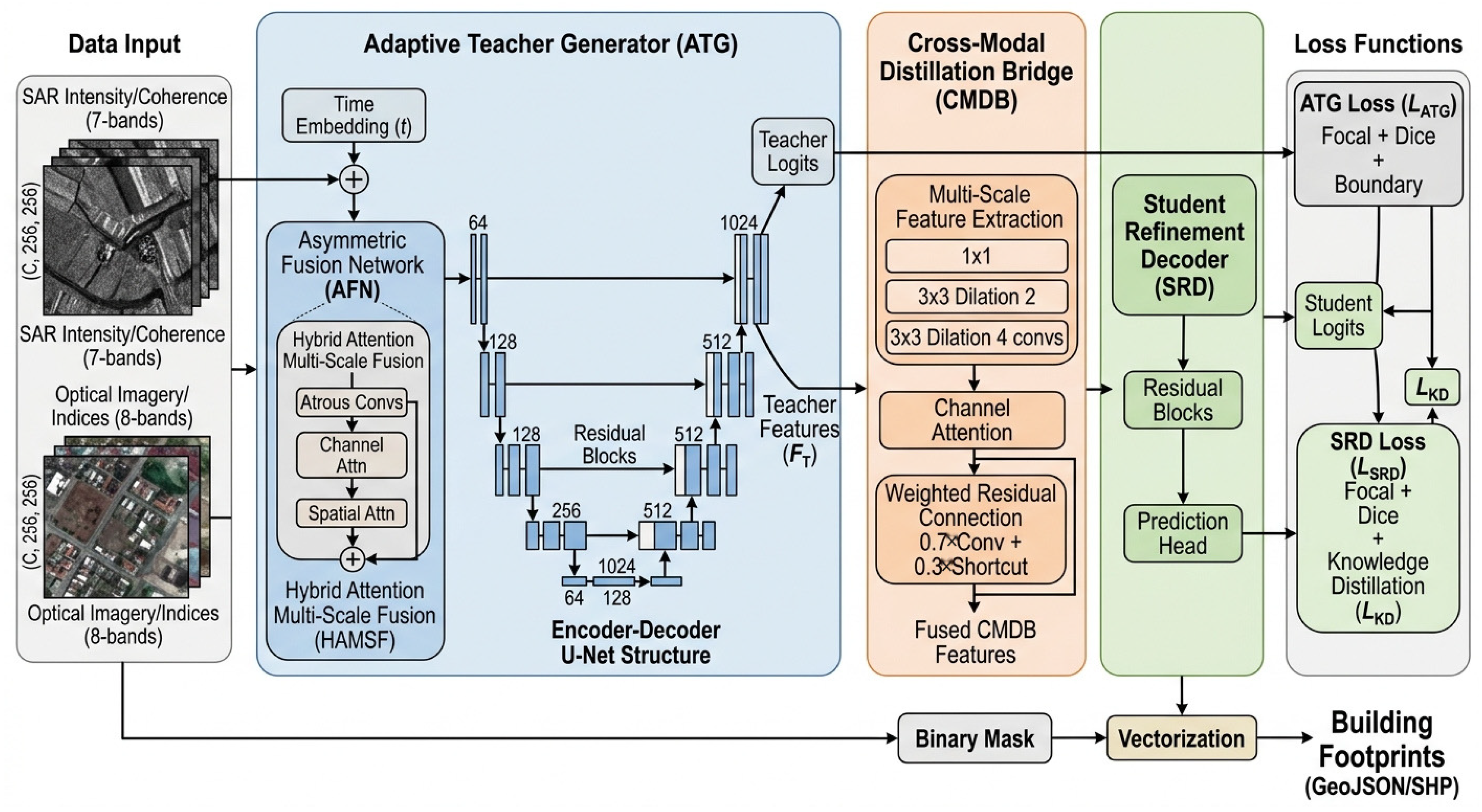
ACBDT is designed as a teacher–student framework for Sentinel-1/Sentinel-2 building-footprint extraction. As shown in Figure 2, the workflow proceeds from modality-specific encoding to teacher feature generation, cross-modal distillation, and student decoding. This order is central to the method: SAR and optical features are first allowed to retain their own statistical structure, then the teacher learns a fused representation, and only after that does CMDB transform and compress this representation into a compact form for downstream decoding by the SRD [20,21,35,37,57].
Figure 2. Overall ACBDT architecture. Sentinel-1 SAR and Sentinel-2 optical channels are encoded separately, fused in the time-step-conditioned teacher, transformed by CMDB, and decoded by SRD. The inference forward pass executes the teacher, CMDB, and SRD; the framework is asymmetric in its supervision structure rather than a student-only deployment graph.
Remotesensing 18 02868 g002
Figure 2 also clarifies why the method is described as asymmetric. The teacher sees the richer fused representation and provides both logits and intermediate features, whereas the student receives the distilled representation generated by CMDB. This structure provides the SRD with a compact cross-modally aligned representation while retaining boundary-sensitive information learned by the teacher. The subsequent equations formalize this mapping and define the tensors used by each component.
During training, ground-truth masks supervise both teacher and student predictions, and distillation transfers teacher information to the student logits. During inference, the same three components are executed deterministically at t = 0. The asymmetry of the design lies in the supervision direction rather than in the deployed graph: the teacher receives the richer objective, and the student is optimized to reproduce its behavior through a compact representation. A branch-separable variant, in which the teacher could be discarded at inference, is identified as future work in Section 6 and is not claimed here.
Formally, let the SAR input be denoted as X sar R B × C s × H × W and the optical input as X opt R B × C o × H × W , where C s =   7 and C o =   8 . The overall mapping of ACBDT can be written as
Y = F SRD F CMDB ( F ATG ( X sar , X opt , t ) ) ,
where t denotes the stochastic time-step conditioning index, sampled during training and fixed at t = 0 during inference, and Ŷ is the final building-probability map. The index t is not defined as a physical noise level or as a monotonic perturbation intensity.

3.2. Adaptive Teacher Generator

3.2.1. Asymmetric Fusion Network

A symmetric encoder would force SAR and optical inputs into a common representation before their noise distributions and semantic roles have been separated. This is undesirable because SAR is governed by scattering geometry and speckle, whereas optical reflectance carries material and vegetation-water-impervious contrast. ACBDT therefore uses separate branches before fusion, allowing each modality to contribute through the evidence it represents best [9,10,26].
The SAR branch takes X sar as input and maps it into a latent space of dimension d / 2 , while the optical branch independently projects X opt to another d / 2 -dimensional representation. The two branches share the same topology but do not share parameters:
F sar   =   ϕ sar ( X sar ) , F opt   =   ϕ opt ( X opt ) ,
where ϕ sar ( ) and ϕ opt ( ) each consist of two 3   ×   3 convolutions, Group Normalization, and SiLU activation. The modality-specific features are concatenated along the channel dimension:
F fused   =   [ F sar ; F opt ] R B × d × H × W ,
where d = 128 in our implementation.
This asymmetric encoding delays cross-modal interaction until each branch has produced a stable feature representation. The design is intended to reduce premature homogenization, which is a common source of confusion when SAR bright targets and optically bright non-building surfaces are treated as equivalent evidence.

3.2.2. Hybrid Attention Multi-Scale Fusion

Buildings in the YRD range from small residential blocks to large industrial roofs, so a single receptive-field size is unlikely to represent all building contexts. HAMSF combines atrous context, channel reweighting, spatial attention, and diffusion-inspired time-step conditioning inside the teacher. Because the present revision focuses the controlled robustness analysis on CMDB and time-step conditioning, HAMSF is retained as a multi-scale design component but is not presented as an independently established source of performance gain [23,43,44,58].
First, a four-branch atrous convolution block with dilation rates r { 1 , 2 , 4 , 6 } is used to extract multi-scale context:
M r   =   δ GN ( Conv 3 × 3 ( r ) ( F fused ) ) , r { 1 , 2 , 4 , 6 } ,
M ms = [ M 1 ; M 2 ; M 4 ; M 6 ] ,
where δ ( ) denotes the SiLU activation.
Channel attention is then applied to emphasize informative semantic channels:
w ca   =   σ W 2 ReLU ( W 1 GAP ( M ms ) ) , M ca   =   M ms w ca ,
where GAP ( ) denotes global average pooling, σ ( ) is the sigmoid function, and is element-wise multiplication.
Next, spatial attention is employed to highlight building-relevant regions:
w sa   =   σ Conv 7 × 7 [ AvgPool ( M ca ) ; MaxPool ( M ca ) ] , M sa   =   M ca w sa .
A diffusion-inspired sinusoidal time-step embedding e_t is then projected and injected into the fused representation:
F hamsf   =   δ GN ( Conv 1 × 1 ( M sa ) ) + W t e t + F fused .
The residual connection preserves the original modality-fused representation and stabilizes optimization.

3.2.3. Time-Step-Conditioned Teacher Network

The Adaptive Teacher Generator (ATG) uses a U-Net-style encoder–decoder with stochastic time-step conditioning. The input to the teacher is the HAMSF-enhanced feature map. Four encoder stages capture increasingly abstract SAR-optical semantics, and the decoder restores spatial detail through skip connections. During training, the sampled time-step index is embedded and added to intermediate teacher features as a conditioning signal. At inference, the ATG remains in the forward graph and is evaluated once with t = 0; its output representation is subsequently transformed by CMDB and decoded by SRD [37,38,39,59].
For a generic residual block, the time-conditioned transformation is formulated as
h 1 = δ GN ( Conv 3 × 3 ( x ) ) ,
h 2   = h 1 + W time e t 1 H × W ,
h out = δ GN ( Conv 3 × 3 ( h 2 ) ) + Conv 1 × 1 ( x ) ,
where h denotes the input feature map and the projected time embedding is spatially broadcast before fusion. The time embedding changes the conditioning state of the residual block but does not itself define a prescribed noise magnitude.
The decoder progressively restores spatial resolution through transposed convolution and skip connections from the corresponding encoder stages. The final teacher classifier produces single-channel binary logits Z_T ∈ R^(B × 1 × H × W). Building probabilities are obtained with a sigmoid function, P_T = σ(Z_T). In addition to Z_T, the last-stage decoder feature map H_T is retained as an intermediate semantic representation for feature-level distillation.
During training, the conditioning index t is randomly sampled from a discrete uniform distribution,
t U ( 0 , T ) ,
and encoded using a sinusoidal embedding. At inference, t is fixed at 0 as a deterministic reference condition. Importantly, the implemented mechanism does not define an explicit forward noising transformation, does not use a beta/noise schedule, and does not learn or execute a reverse diffusion process. Consequently, t indexes a conditioning vector rather than a prescribed perturbation magnitude, and larger t should not be interpreted as a stronger perturbation. The mechanism is therefore referred to throughout this revision as diffusion-inspired time-step conditioning rather than as a diffusion model. The controlled ‘w/o time-step conditioning’ variant removes every projected e_t term from HAMSF and the ATG residual blocks during both training and inference.

3.3. Cross-Modal Distillation Bridge

The teacher features produced by ATG are informative but redundant for direct decoding. CMDB is therefore introduced as the methodological core of ACBDT: it transforms high-capacity teacher semantics into a compact representation while preserving the cross-modal alignment learned from the SAR and optical branches. Its role is evaluated in Section 4.5.2 by a controlled CMDB-bypass configuration trained independently under the same spatial split and optimization protocol as the full model. This key ablation is repeated across three random seeds and reported as mean ± standard deviation, so the bridge-associated change is evaluated against run-to-run variability rather than from a single frozen checkpoint.
Given the teacher feature map F T , CMDB first applies progressive multi-scale feature extraction using serial dilated convolutions:
F 1   =   ψ Conv 3 × 3 ( 1 ) ( F T ) ,
F 2 = ψ Conv 3 × 3 ( 2 ) ( F 1 ) ,
F 3 = ψ Conv 3 × 3 ( 4 ) ( F 2 ) ,
F conv = ψ Conv 1 × 1 ( F 3 ) ,
where ψ ( ) denotes the GELU activation followed by Group Normalization.
A lightweight channel attention mechanism is then introduced to suppress redundant responses and emphasize distillation-critical channels:
A ch   =   σ Conv 1 × 1 ( GELU ( Conv 1 × 1 ( GAP ( F conv ) ) ) ) ,
F att =   F conv A ch .
To preserve the semantic continuity between teacher and student representations, a weighted residual connection is adopted:
F CMDB   =   Conv 1 × 1 ( 0.7 F att   +   0.3 F T ) .
The resulting F CMDB is a compact distilled feature map that serves as the input to the student decoder. The asymmetric weighting strategy biases the bridge toward transformed distillation features while retaining part of the original teacher semantics, thereby reducing distributional shock during early training.

3.4. Student Refinement Decoder

The Student Refinement Decoder (SRD) converts the distilled CMDB feature map into the final building probability map. Its role is deliberately narrower than that of the teacher: rather than relearning cross-modal fusion, it operates on the compact representation generated by CMDB to refine spatial detail and preserve building boundaries. This compact decoding design limits the additional decoding overhead after cross-modal feature generation and supports tiled city-scale inference [20,21,22,23].
The SRD takes F CMDB as input and processes it through a cascade of residual refinement blocks (RRBs). Each RRB consists of two 3   ×   3 convolutions with Group Normalization and SiLU activation, plus a 1 × 1 shortcut:
F k + 1   =   δ GN Conv 3 × 3 ( δ ( GN ( Conv 3 × 3 ( F k ) ) ) )   +   Conv 1 × 1 ( F k ) .
The channel widths are gradually reduced from 128 to 64 and then to 32, allowing progressive refinement and compression.
To strengthen edge localization, a boundary enhancement branch is inserted after the second refinement block:
F bnd   =   λ b δ ( Conv 3 × 3 ( F RRB 2 ) ) ,
F enh = F RRB 2 +   F bnd ,
where λ b is a learnable scalar initialized to zero. This conservative initialization ensures that the student first learns stable distilled semantics before emphasizing boundary-sensitive responses.
Finally, the refined feature map is passed through dropout and a 1 × 1 classifier to produce single-channel student logits Z_S ∈ R^(B × 1 × H × W). The final building-probability map is obtained as Ŷ = σ(Z_S):
Z S   =   Conv 1 × 1 ( Dropout ( F RRB 3 ) ) , Y S   =   σ ( Z S ) ,
where Ŷ denotes the final foreground probability map, and thresholding is applied only for binary mask evaluation.

3.5. Loss Functions and Training Strategy

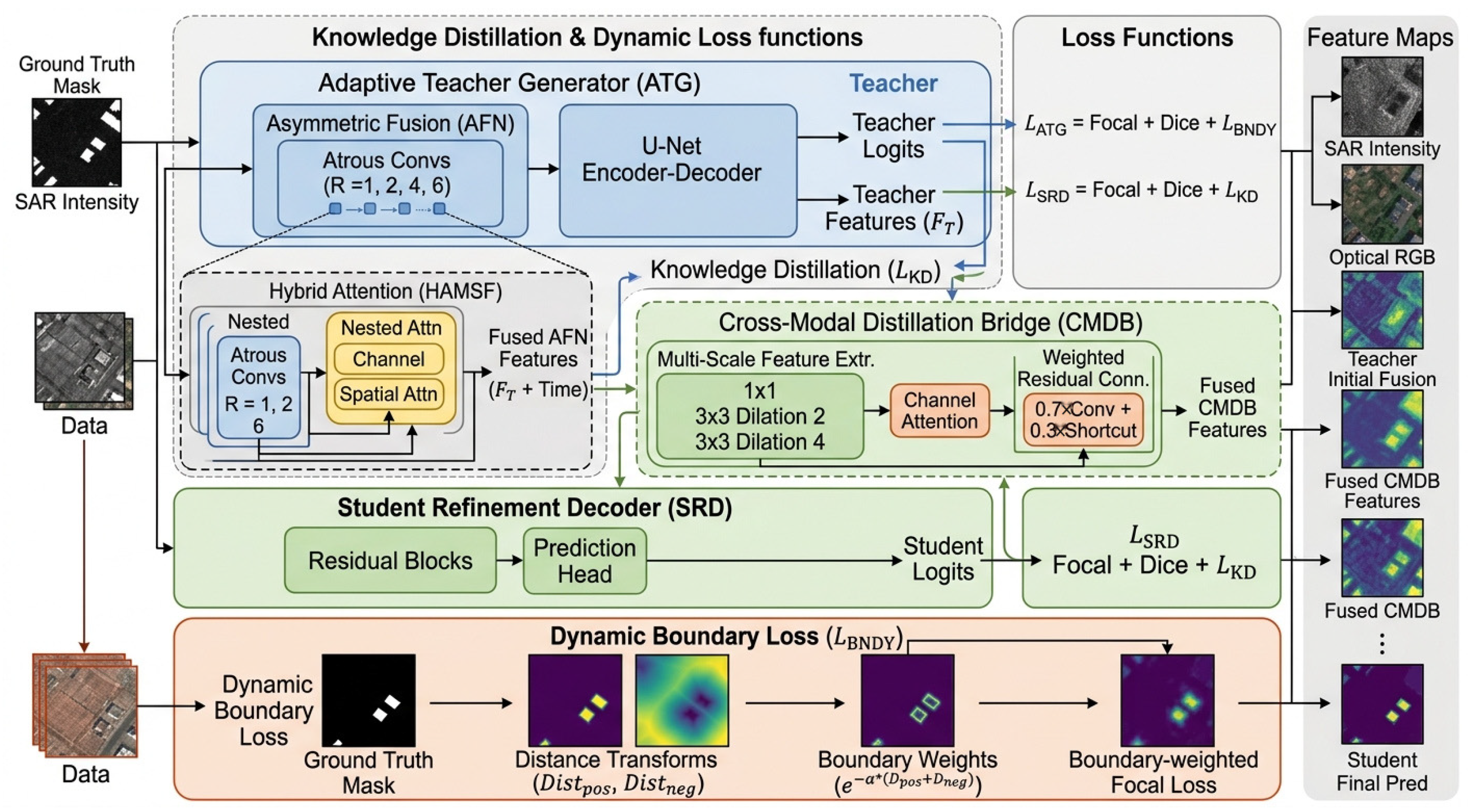
Figure 3 separates the supervision sources used by ACBDT. Teacher supervision stabilizes the high-capacity branch, student supervision anchors the final prediction branch to the reference masks, and distillation transfers teacher logits and features through CMDB. The boundary-aware term is included because the dominant practical errors in building extraction are often edge displacement and mixed-pixel omission rather than whole-object absence. The following equations define these losses before they are combined into the final objective [60,61].
Figure 3. Training mechanism of ACBDT. Teacher, student, distillation, and boundary-aware losses are coupled during training so that the SRD output branch inherits cross-modal and boundary-sensitive information from the teacher representation.
Remotesensing 18 02868 g003

3.5.1. Teacher Supervision

The teacher loss is composed of focal loss, Dice loss, and a boundary-aware loss:
L T   =   λ FL T L FL T   +   λ Dice T L Dice T   +   λ B T L B T .
The focal loss is defined as
L FL = 1 N i = 1 N α t ( 1     p t , i ) γ log ( p t , i ) ,
where α t = 0.25 and γ = 2 .
The Dice loss is
L Dice = 1     2 i = 1 N p i y i + ϵ i = 1 N p i + i = 1 N y i + ϵ .
To emphasize difficult boundary pixels, we introduce a boundary-aware weighting term derived from distance transforms:
w i   =   1   +   β exp d i 2 2 σ d 2 ,
where d i measures the distance from pixel i to the nearest boundary, β controls the weight amplitude, and σ d controls the spatial decay. The boundary-aware supervision can then be written as
L B = 1 N i = 1 N w i y i log ( p i ) + ( 1     y i ) log ( 1     p i ) .
In our implementation, λ FL T   =   0.4 , λ Dice T   =   0.4 , and λ B T   =   0.2 .

3.5.2. Knowledge Distillation [35,36]

To transfer both predictive behavior and internal semantics from teacher to student, two complementary distillation objectives are used. The teacher and student segmentation heads are explicitly binary and output single-channel logits, Z_T,Z_S ∈ R^(B×1×H×W). Therefore, channel-wise Softmax is not used for logit distillation, because Softmax over a one-channel tensor is identically one and would make the KL term degenerate.
For logit distillation, temperature-scaled Bernoulli probabilities are defined as p_T = σ(Z_T/T) and p_S = σ(Z_S/T). The soft-logit term is the pixel-wise KL divergence between the corresponding Bernoulli distributions:
Lkdlogit = (T2/N) Σi { p_T,i ln[(p_T,i+ε)/(p_S,i+ε)] + (1−p_T,i) ln[(1−p_T,i+ε)/(1−p_S,i+ε)] }
Here, T is the distillation temperature, set to 3, N is the number of evaluated pixels, and ε = 1 × 10⁻⁷ is used for numerical stability. Multiplication by T2 preserves the gradient scale under temperature smoothing. This formulation is mathematically consistent with the single-channel sigmoid segmentation heads.
The second term is a feature-level distillation objective that aligns the student intermediate representation with the corresponding teacher representation after dimensional alignment. Teacher features are used as stop-gradient targets. Its isolated contribution is not claimed because a separate feature-distillation removal experiment is not included in the present study.
L FD = 1 CHW F mid T     F mid S 2 2 .
The total distillation loss is
L KD = λ SLD L SLD +   λ FD L FD ,
where λ SLD   =   0.6 and λ FD   =   0.4 .

3.5.3. Student Supervision and Overall Objective

The student is supervised by both hard labels and teacher guidance. Its total loss is defined as [60,61]
L S = ( 1     α KD ) L hard S + α KD L KD ,
where α KD   =   0.4 . The hard-label term L hard S adopts the same combination of focal, Dice, and boundary-aware components as the teacher, but with different weights:
L hard S = λ FL S L FL S + λ Dice S L Dice S + λ B S L B S ,
where λ FL S   =   0.3 , λ Dice S   =   0.5 , and λ B S   =   0.2 .
The overall training objective is therefore
L total = L T + L S .
Gradient propagation is explicitly one-way. The teacher logits and teacher feature targets are detached before the distillation losses are evaluated. Accordingly, the teacher parameters θ_T are updated only by the teacher supervision loss L_T, whereas the CMDB and student parameters are updated by the student hard-label loss and the logit/feature distillation losses; ∂L_distill/∂θ_T = 0. This stop-gradient implementation prevents reciprocal student-to-teacher adaptation and keeps the supervisory direction consistent with the mathematical formulation.

3.6. Training and Inference Protocol

The training configuration was held fixed across ACBDT and all same-protocol baselines. Optimization used AdamW with an initial learning rate of 1 × 10⁻⁴, weight decay 1 × 10⁻⁴, beta1 = 0.9, and beta2 = 0.999. The learning rate followed cosine annealing with warm restarts (T0 = 15 epochs, Tmult = 2, minimum learning rate 1 × 10⁻⁶). Training ran for 400 epochs at a batch size of 4 with automatic mixed precision. Augmentation was applied to the training partition only and comprised horizontal and vertical flips, 90-degree rotations, random scaling and cropping, multiplicative speckle perturbation of the SAR channels, brightness and contrast jitter of the optical channels, and additive Gaussian noise. Weighted sampling oversampled patches with a building fraction above 0.1. No external pretraining was used, since no pretrained weights exist for the 15-channel SAR-optical input. All baselines in Section 4.5.1 used the same optimizer, schedule, batch size, epoch budget, augmentation, sampling, and checkpoint-selection rule; only the architecture and the input-adapter layer differed. Experiments used PyTorch 2.1.2 with CUDA 12.1 on a single NVIDIA GeForce RTX 4090 GPU with 24 GB of memory.
During inference, the model is evaluated deterministically with the time-step conditioning index fixed at t = 0. The teacher generator, CMDB, and SRD are each executed once in the forward pass. No iterative diffusion sampling is performed. ACBDT is therefore asymmetric in supervision structure rather than a student-only deployment graph. Section 4.5.3 reports the retained direct implementation record for the archived ACBDT checkpoint. Cross-model GMAC, memory, and latency comparisons are not reported because the retained revision materials do not substantiate direct same-hardware measurements for the baseline models.

3.7. Benchmark and Validation Protocol

The benchmark comparison in Section 4.5.1 follows a same-protocol design. All baseline architectures were trained from scratch by the authors on the identical patch inventory, SAR-optical preprocessing chain, reference masks, spatial train/validation/test partition, patch size, optimizer, learning-rate schedule, augmentation policy, epoch budget, and checkpoint-selection rule described in Section 3.6, and all methods were scored with a single shared metric implementation. Multimodal baselines were adapted to accept the 15-channel SAR-optical stack, whereas the modality-restricted U-Net variants received the corresponding eight-channel optical or seven-channel SAR inputs. The comparison is therefore a controlled within-study evaluation on a common test partition; it is not a claim about published leaderboard results obtained under different datasets and training recipes.
The broad same-protocol benchmark is retained as a reference comparison. To quantify run-to-run variability for the reviewer-identified critical comparisons, three independent training runs are specified for ACBDT, the strongest baseline (FTransUNet), ACBDT without CMDB, and ACBDT without time-step conditioning, using the same fixed spatial train/validation/test partition and the same training protocol while varying random initialization and stochastic data order (seeds 42, 123, and 2026). The repeated-seed analysis reports these four configurations as mean ± standard deviation on the held-out test partition. The remaining baseline records remain single-run reference records and are not assigned variance-based claims.
Metric definitions are stated explicitly so that the reported values can be reproduced. Overall accuracy, precision, recall, F1-score, IoU, and Cohen’s Kappa are computed for the building class unless stated otherwise [62,63,64]. Cohen’s Kappa is reported in the text and tables as a unitless coefficient on the 0–1 scale, not as a percentage. In Figure 4b and Figure 5c, where Kappa is overlaid with percentage-valued metrics on a common axis, the plotted quantity is explicitly labeled 100×Kappa. Boundary F1 (BF1) follows contour matching: reference and predicted boundaries are extracted by morphological gradient; a predicted boundary pixel is matched when a reference boundary pixel lies within a 3-pixel tolerance (30 m at 10 m ground sampling); boundary precision and recall are combined by their harmonic mean [65,66]. The benchmark and repeated-seed analyses use dataset-level BF1 from boundary-pixel counts pooled across tiles.
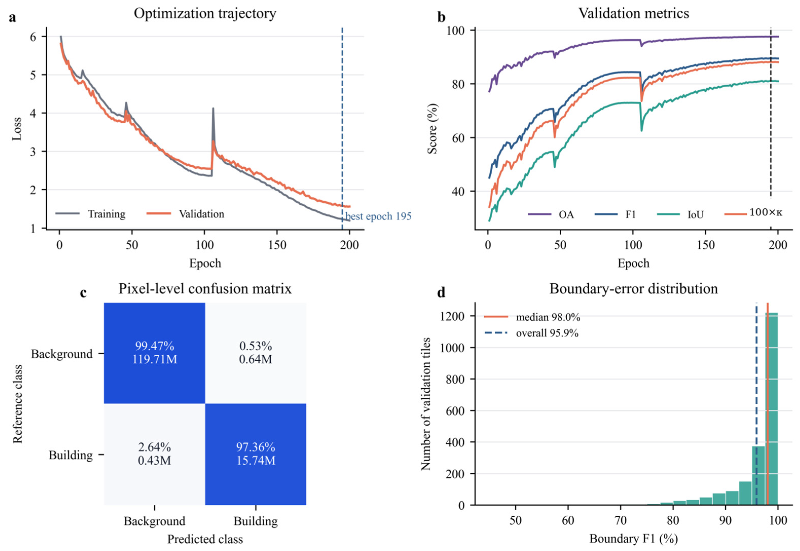
Figure 4. ACBDT training and validation diagnostics. (a) Training loss (gray) and validation loss (orange); the blue dashed line marks the selected checkpoint. (b) Validation overall accuracy (purple), F1-score (blue), building IoU (green), and 100×Kappa (orange) on a common percentage scale; the black dashed line marks the selected checkpoint. (c) Row-normalized pixel-level confusion matrix from the post-training evaluation. (d) Tile-level boundary-F1 distribution (green bars), with the orange solid line indicating the median and the blue dashed line indicating the pooled overall BF1.
Remotesensing 18 02868 g004
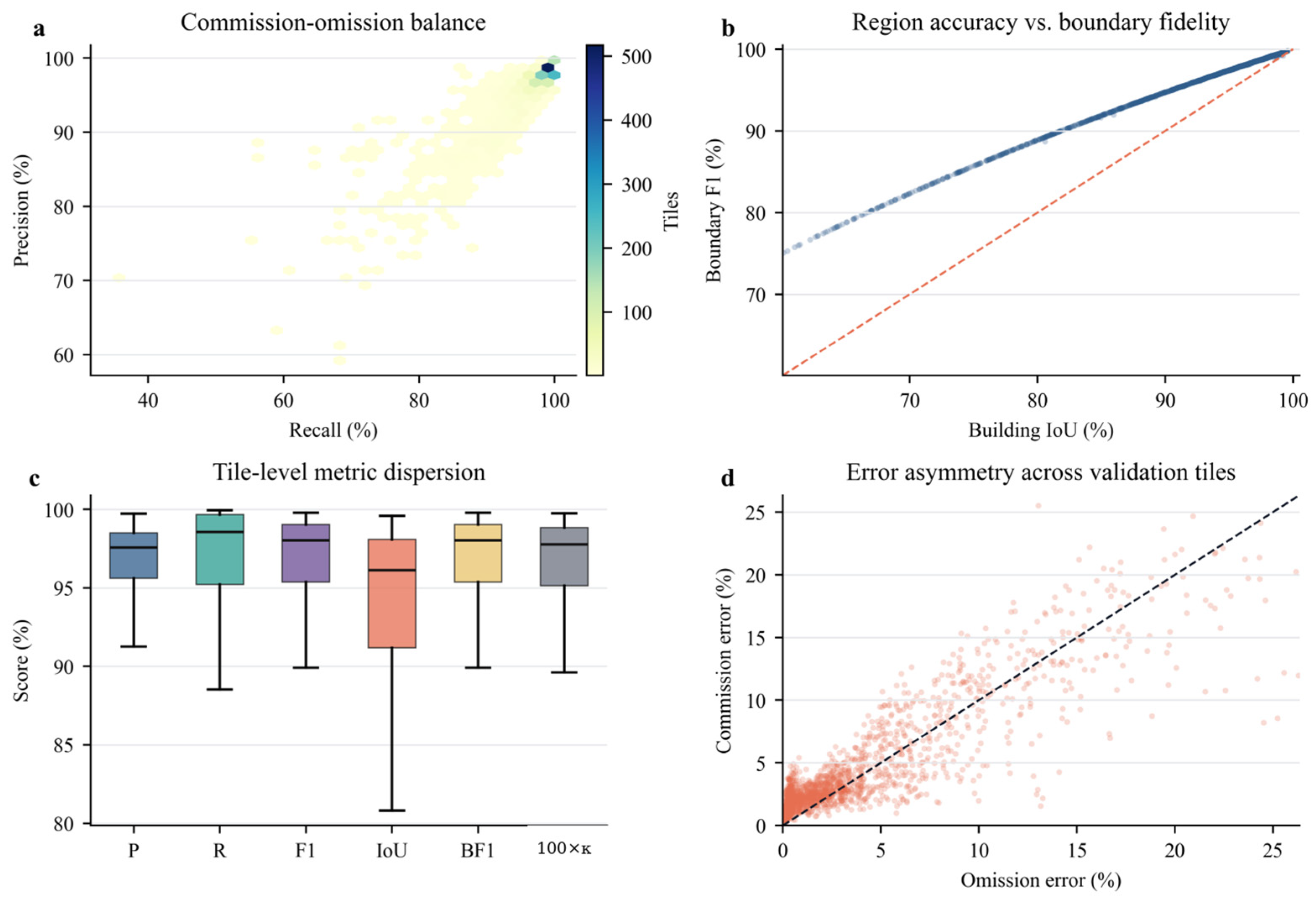
Figure 5. Validation error profile. (a) Tile-level precision-recall density; the color scale indicates the number of tiles per bin. (b) Building IoU versus boundary F1; blue points show validation tiles and the orange dashed line is the 1:1 reference. (c) Dispersion of tile-level precision (P), recall (R), F1, IoU, boundary F1 (BF1), and 100 × Kappa. (d) Commission versus omission error; coral points show validation tiles and the black dashed line is the 1:1 reference (equal commission and omission).
Remotesensing 18 02868 g005
The primary split is spatially disjoint within the eight-city inventory, which removes the near-duplicate adjacency that inflates randomly partitioned accuracy [55,56]. However, it does not remove between-city differences in morphology, terrain, and acquisition geometry, because every city contributes patches to every partition. Fully held-out city experiments are not reported in this study. The consequence is stated rather than left implicit: the reported accuracies estimate performance on unseen ground within the Yangtze River Delta under the sensing conditions sampled here, and they do not estimate performance on a city absent from training. No out-of-city transfer claim is made anywhere in this manuscript, and leave-one-city-out validation is identified in Section 5.3 as the specific experiment required before such a claim would be admissible.

4. Results and Analysis

The results are ordered to match the claims made in the manuscript. Training diagnostics first establish checkpoint stability. Pixel- and tile-level error decomposition then identifies omission, commission, and boundary behavior. Representative samples and city-scale maps assess spatial plausibility. Finally, the broad same-protocol benchmark, repeated-seed robustness and key ablations, implementation audit, and density-stratified analysis establish overall performance and the scope of the component-level evidence. Table 5 records the inventory, partition, aggregation rule, and evidential role underlying each quantitative record.
Table 5. Evaluation ledger recording the inventory, partition, aggregation rule, and evidential role of each quantitative record.
RecordInventoryPartitionAggregationReported RecordHeadline UseEvidential Role
Checkpoint-selection log2680-patch eight-city setValidationTile-aggregatedOA 97.60; IoU 81.08; F1 89.55; Kappa 0.8819NoCheckpoint selection only
Pixel-pooled diagnostic2083-tile single-city archiveFull archive (136,511,488 px)Pixel-pooled (micro)OA 99.22; Precision 96.09; Recall 97.36NoError diagnosis only; not comparable with tile metrics
Same-protocol benchmark2680-patch eight-city setHeld-out testTile-aggregated; dataset BF1OA 95.47; IoU 85.63; F1 92.24; Kappa 0.9017; BF1 83.71ReferenceBroad architecture comparison; single-run values
Repeated-seed robustness and key ablations2680-patch eight-city setHeld-out testTile-aggregated; dataset BF13 runs each: ACBDT, FTransUNet, w/o CMDB, w/o time-stepYesMean ± SD robustness evidence
ACBDT implementation (Section 4.5.3)Archived ACBDT checkpointInference recordDirect ACBDT profiling32.402 M; 33.80 ± 4.31 ms/tile; 11,633.6 km2/minNoACBDT only; no cross-model efficiency claim
Density diagnosticSame 416-tile auditFive density strataTile-aggregated by stratumFull model > optical-only in all strataNoObserved density dependence of SAR contribution

4.1. Training Convergence and Evaluation Protocol

ACBDT was trained for 400 epochs, and the deployed checkpoint was selected by Kappa on the validation partition, which is disjoint from the test partition used for all reported accuracies. Training and validation loss curves decline smoothly, and the validation metrics plateau well before the selected checkpoint (Figure 4), indicating that the selection point is not an outlier of an unstable trajectory. Because selection uses the validation partition alone, the test-partition values in Section 4.5 are free of selection bias from test-set monitoring. For transparency, the validation log at the selected checkpoint reported 97.60% overall accuracy, 81.08% building IoU, 89.55% F1-score, and Kappa = 0.8819; these are optimization records and are not compared directly with test-partition values.
The evaluation ledger separates quantities produced under different protocols. The checkpoint and pixel-pooled records support optimization and error diagnosis; the broad same-protocol architecture comparison provides the reference benchmark; the repeated-seed analysis provides robustness and key-ablation evidence; Section 4.5.3 provides direct ACBDT implementation profiling; and the density analysis provides the modality diagnostic. This separation prevents numerical comparisons across incompatible inventories or aggregation rules.

4.2. Pixel-Level and Tile-Level Error Structure

Once checkpoint stability is established, the next question is the composition of the residual error. The pixel-pooled diagnostic in Table 6 aggregates 136,511,488 pixels, which corresponds to the full 2083-tile single-city diagnostic archive rather than to the 268-tile test partition; the two inventories are listed separately in Table 5 for this reason. The pixel count exactly equals 2083 × 256 × 256 = 136,511,488, confirming that this pixel-pooled diagnostic was computed over the full 2083-tile archive. Row-normalized interpretation gives a background-to-building commission rate of 0.53% and a building omission rate of 2.64%, so the model is not trading one error type for the other. These are micro-averaged rates that characterize error structure; they run higher than tile-aggregated metrics because dense tiles dominate the pixel pool, and they are consequently never compared with Table 7.
Table 6. Pixel-pooled (micro-averaged) confusion matrix from the diagnostic evaluation, used for commission and omission error analysis only. This micro-averaged record is aggregated over pixels rather than tiles and is therefore not directly comparable with the tile-aggregated metrics in Table 7, Table 8 and Table 9.
Reference/PredictionPredicted BackgroundPredicted Building
Reference background119,707,039639,784
Reference building427,31415,737,351
Figure 5 extends Table 6 diagnosis from pixels to mapping units. Most validation tiles cluster near high precision and high recall, but the IoU distribution still has a low-score tail. Boundary F1 rises and falls with building IoU, showing that regional detection and edge quality are coupled in difficult patches. The commission-omission scatter further indicates that hard tiles often contain both error types, which is consistent with mixed roof-road pixels, small isolated buildings, and weak optical or scattering contrast. These observations justify the qualitative inspection that follows [62,63,64,66].

4.3. Qualitative Assessment of Representative Validation Samples
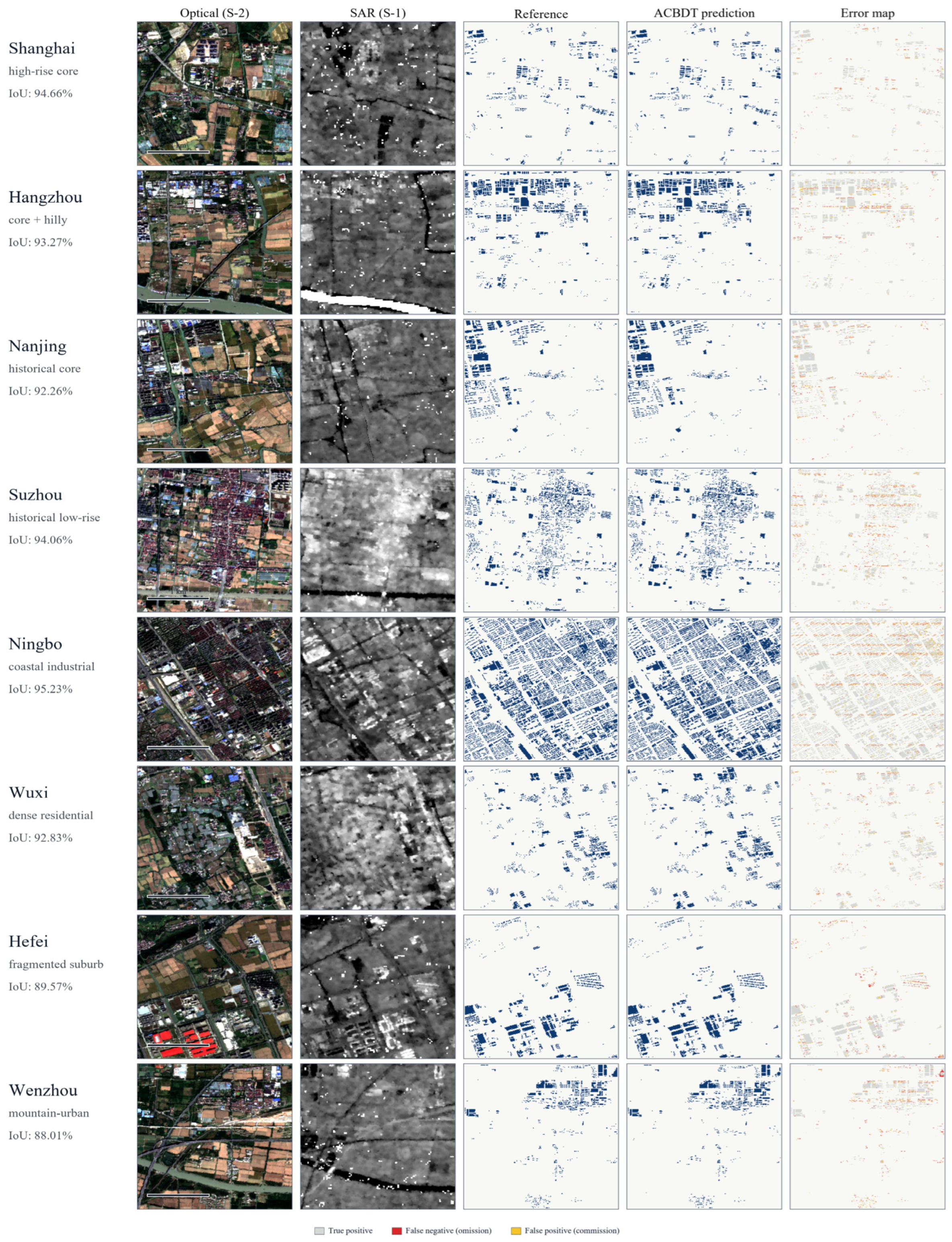
The preceding metrics quantify error magnitude, but they cannot show whether the predicted masks are spatially plausible. Figure 6 therefore compares Sentinel-2 composites, Sentinel-1 SAR composites, reference masks, ACBDT predictions, and error maps for representative scenes from the eight YRD cities. The selected examples cover high-rise cores, historical low-rise districts, dense residential neighborhoods, coastal industrial zones, fragmented suburbs, and mountain-urban transition areas.
Figure 6. Representative validation samples across eight Yangtze River Delta cities. Each row shows Sentinel-2 optical input, Sentinel-1 SAR input, reference mask, ACBDT prediction, and error map. In the error maps, gray denotes true positives, red denotes false negatives (omission), and yellow denotes false positives (commission); the same color key is shown at the bottom of the figure [4,5,24,25].
Remotesensing 18 02868 g006
Across the examples, ACBDT preserves the dominant building clusters and maintains visible separation along roads, open spaces, and internal gaps. Sample-level IoU ranges from 88.01% in the Wenzhou mountain-urban scene to 95.23% in the Ningbo coastal industrial scene. The stronger examples are those where optical roof contrast and SAR structural texture reinforce one another, especially in compact or regularly arranged industrial and residential blocks.
The error maps identify where the method remains fragile. False negatives occur mainly in small isolated structures, narrow courtyards, and fragmented residential clusters, while false positives appear near mixed roof-road or impervious-surface pixels. In Wenzhou, terrain and SAR geometric distortion weaken the agreement between scattering texture and optical building evidence. These errors follow the 10 m resolution and SAR-geometry limits described in Section 2, which is why the next subsection checks whether such local behavior remains controlled during city-scale inference.

4.4. City-Scale Building Extraction Across the Yangtze River Delta
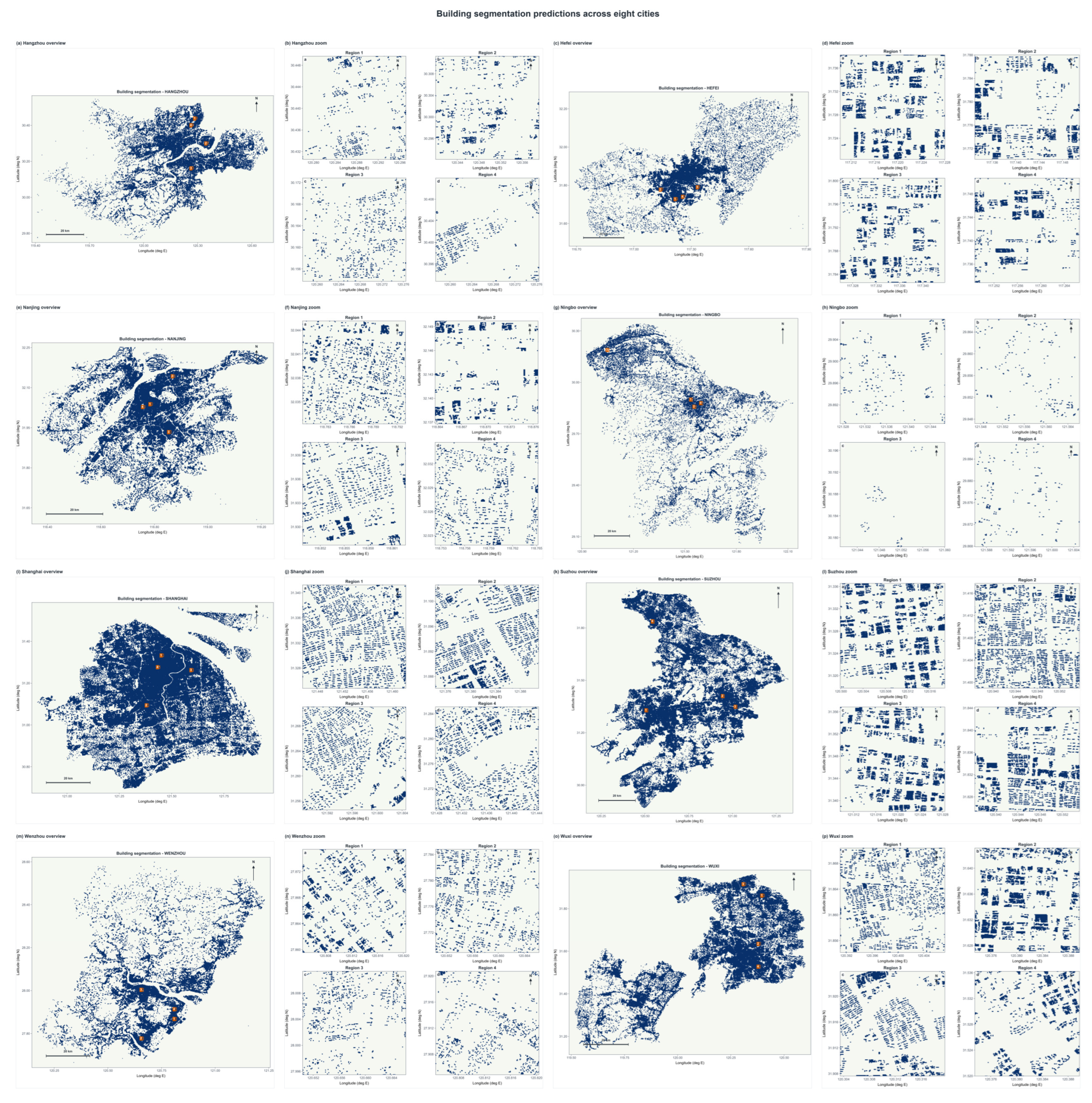
The representative samples test local behavior, but operational building mapping also requires spatially continuous predictions. Figure 7 therefore evaluates a different property: whether tiled inference produces coherent city-scale building patterns without obvious discontinuities. Across Hangzhou, Hefei, Nanjing, Ningbo, Shanghai, Suzhou, Wenzhou, and Wuxi, predicted masks form continuous urban structures rather than isolated noisy fragments.
Figure 7. City-scale ACBDT building-extraction maps and zoomed detail panels for eight Yangtze River Delta cities. Blue masks indicate predicted building footprints, and orange markers identify the zoomed regions. These maps are used as qualitative evidence of spatial continuity and are not treated as an independent accuracy assessment.
Remotesensing 18 02868 g007
The overview panels show dense central concentrations, lower-density outward gradients, and corridor-like development along transport and river systems, all consistent with the urban forms introduced in Section 2. The zoomed panels show that the model can represent both large regular roof blocks and finer residential fabrics. This spatial behavior is consistent with the architecture: separate SAR-optical encoding limits early modality conflict, multi-scale processing accommodates roof-size variation, and SRD preserves local boundary structure [2,3,53,67].
The city-scale maps are visual and spatial evidence, not an independent accuracy assessment. They show that the trained model can be applied continuously over large extents without visible tiling artifacts, but they do not replace validation against external reference data. The areas with the greatest residual uncertainty are fragmented peri-urban settlements and terrain-affected margins; these are also the conditions examined in the density-stratified analysis.

4.5. Quantitative Evaluation: Benchmark Comparison and Observed Diagnostics

4.5.1. Overall Benchmark Comparison

The preceding subsections established convergence behavior, error structure, sample-level plausibility, and city-scale mapping coherence. Table 7 reports the broad reference benchmark: a controlled comparison of ACBDT with eight representative segmentation baselines under one shared data split, preprocessing pipeline, input configuration, training protocol, and metric implementation. Modality-restricted U-Net variants examine the effect of input modality at fixed architecture; convolutional encoder–decoders and Transformer segmentation networks [21,23,24] provide strong single-stream references; CMX [68] and FTransUNet [69] provide explicit cross-modal fusion comparisons; and DiffusionSeg provides a diffusion-based reference [33,34]. Because Table 7 retains one archived run per method, its pairwise differences are descriptive. The reviewer-requested run-to-run robustness analysis is reported separately in Table 8 for ACBDT, FTransUNet, and the two critical ablations.
Table 7. Same-protocol single-run reference benchmark on the held-out eight-city test partition. All methods use the identical data split, preprocessing chain, augmentation policy, optimizer, schedule, checkpoint-selection rule, and metric implementation. BF1 is dataset-level at a 3-pixel tolerance. The ACBDT-versus-FTransUNet robustness comparison is evaluated independently across three runs in Table 8.
MethodModalityOA (%)IoU (%)F1 (%)KappaBF1 (%)Params (M)
U-Net (OPT)OPT92.1474.8385.620.813472.3131.0
U-Net (SAR)SAR89.6768.2481.130.758965.4731.0
DeepLab v3+ (CAT)OPT + SAR93.2877.5687.340.836774.8259.3
HRNet (FUSE)OPT + SAR93.7178.9388.190.847876.1465.8
SegFormer (B3)OPT + SAR94.1280.4789.210.861277.5347.2
CMXOPT + SAR94.5682.1390.170.874379.6873.4
FTransUNetOPT + SAR94.8383.2790.840.882181.2388.6
DiffusionSegOPT + SAR94.3181.7989.940.869878.9494.2
ACBDT (Ours)OPT + SAR95.4785.6392.240.901783.7132.402
In the retained single-run reference benchmark, FTransUNet is the strongest baseline at 83.27% IoU and 81.23% BF1 [69], while ACBDT records 85.63% IoU and 83.71% BF1, corresponding to observed single-run differences of 2.36 and 2.48 percentage points. These values are retained only to preserve the full architecture comparison and are not treated as variance-supported superiority estimates. The repeated-seed comparison in Table 8 provides the appropriate robustness evidence for ACBDT relative to FTransUNet.
Boundary F1 is reported because building-footprint products serve urban morphology, exposure modeling, and hazard assessment, where edge fidelity matters alongside area agreement [27,70,71]. Section 4.5.3 reports only the directly retained ACBDT implementation record. The implemented ACBDT forward graph contains 32.402 M trainable parameters. This value supersedes the 62.8 M figure given in the original submission, which was an arithmetic error in the earlier parameter tally; the corrected count was obtained by direct enumeration of trainable parameters in the archived inference graph. The correction is stated explicitly rather than applied silently.

4.5.2. Controlled Ablation and Repeated-Seed Analysis

The single-run benchmark in Section 4.5.1 establishes the observed performance of ACBDT relative to the compared architectures, but it does not quantify run-to-run variability or isolate the contribution of individual components. To address this limitation, we supplemented the benchmark with repeated-seed experiments for the full ACBDT model, the strongest baseline (FTransUNet), ACBDT without CMDB, and ACBDT without time-step conditioning. Each configuration was independently trained three times under the same data partition, preprocessing pipeline, optimizer, learning-rate schedule, augmentation policy, epoch budget, and checkpoint-selection rule. All repeated-seed models were evaluated on the same held-out test partition used in Section 4.5.1, and the results are reported as mean ± standard deviation.
For the CMDB ablation, both SAR and optical inputs were retained while the bridge transformation was bypassed, allowing the effect associated with cross-modal feature transformation to be examined without changing the input information. For the time-step-conditioning ablation, the time-step embeddings and their corresponding feature injections were removed during both training and inference, while the remaining network architecture and optimization settings were kept unchanged. In addition to these principal repeated-seed experiments, the previously retained 416-tile single-seed audit was preserved to examine modality dependence and the secondary HAMSF component. Because the two protocols use different evaluation inventories and numbers of runs, their absolute values are not compared directly.
Table 8. Repeated-seed principal experiments and retained single-seed modality/component diagnostics. Results from the held-out test protocol are reported as mean ± standard deviation over three independent runs. The dagger-marked records are retained single-seed diagnostics on the separate 416-tile audit inventory. ΔIoU is calculated relative to the corresponding full ACBDT configuration within the same protocol.
ConfigurationProtocolRunsIoU (%)ΔIoU (pp)F1 (%)KappaBF1 (%)
Full ACBDTHeld-out test385.61 ± 0.3292.24 ± 0.190.9015 ± 0.002883.74 ± 0.34
FTransUNetHeld-out test383.21 ± 0.24−2.4090.82 ± 0.160.8818 ± 0.002581.19 ± 0.29
w/o CMDBHeld-out test379.01 ± 0.42−6.6088.27 ± 0.310.8546 ± 0.003777.63 ± 0.46
w/o time-step conditioningHeld-out test384.53 ± 0.20−1.0891.62 ± 0.140.8924 ± 0.002182.47 ± 0.26
Full ACBDT †416-tile audit182.790.460.873881.35
Optical only †416-tile audit180.61−2.0989.180.858779.42
SAR only †416-tile audit167.2−15.5080.380.731664.73
w/o HAMSF †416-tile audit181.88−0.8289.940.868180.57
† The modality and HAMSF records are retained as single-seed diagnostics on the separate 416-tile audit inventory and are reported for descriptive interpretation only. They are not numerically compared with the repeated-seed held-out-test results.
The repeated-seed results provide a more robust estimate of the observed difference between ACBDT and the strongest baseline. ACBDT achieves a mean IoU of 85.61 ± 0.32%, compared with 83.21 ± 0.24% for FTransUNet, corresponding to an observed mean difference of 2.40 percentage points. The same ordering is observed for F1, Kappa, and BF1, for which ACBDT reaches 92.24 ± 0.19%, 0.9015 ± 0.0028, and 83.74 ± 0.34%, respectively. The relatively small standard deviations indicate limited run-to-run variation under the present training protocol. Nevertheless, because only three independent runs were conducted, these results are interpreted primarily through their means and dispersion rather than as evidence of formal statistical superiority.
Among the controlled architectural ablations, removing CMDB produces the largest performance degradation. When both sensing modalities are retained, but the bridge transformation is bypassed, mean IoU decreases from 85.61 ± 0.32% to 79.01 ± 0.42%, corresponding to a reduction of 6.60 percentage points. F1 decreases from 92.24 ± 0.19% to 88.27 ± 0.31%, Kappa from 0.9015 ± 0.0028 to 0.8546 ± 0.0037, and BF1 from 83.74 ± 0.34% to 77.63 ± 0.46%. Because the SAR and optical inputs and the remaining training settings are unchanged, this result provides repeated-run evidence that the dedicated transformation performed by CMDB is important for converting the heterogeneous SAR-optical representation into features that can be effectively exploited by the downstream decoder. The magnitude of the change is substantially larger than the run-to-run dispersion observed for the full model.
Removing time-step conditioning produces a smaller but consistent reduction. Without the time-step embedding and its feature injection, mean IoU decreases to 84.53 ± 0.20%, 1.08 percentage points below the full ACBDT result. Corresponding decreases are also observed in F1, Kappa, and BF1. This controlled comparison therefore indicates that time-step conditioning provides an additional performance benefit, but its effect is considerably smaller than that associated with CMDB. Accordingly, the revised manuscript treats this mechanism as an auxiliary conditioning strategy rather than as the dominant source of the model’s improvement.
The retained single-seed modality audit provides complementary information on the relative roles of Sentinel-1 and Sentinel-2. Within the 416-tile diagnostic inventory, the optical-only configuration reaches 80.61% IoU, only 2.09 percentage points below the corresponding full ACBDT record of 82.70%. By contrast, SAR-only input reaches 67.20% IoU, representing a 15.50-point decrease. F1, Kappa, and BF1 exhibit the same general ordering. These results indicate that Sentinel-2 supplies most of the semantic discrimination required for building extraction at 10 m resolution, whereas Sentinel-1 alone is substantially less effective. The improvement of the full multimodal model over the optical-only configuration is therefore consistent with SAR contributing complementary structural information rather than replacing the semantic information provided by the optical observations.
The single-seed HAMSF diagnostic shows a comparatively small change. Removing HAMSF reduces IoU from 82.70% to 81.88%, corresponding to a difference of 0.82 percentage points, with similarly limited changes in F1, Kappa, and BF1. Because this record derives from only one seed and a separate diagnostic inventory, the isolated contribution of HAMSF remains less strongly supported than that of CMDB. HAMSF is therefore retained as a multi-scale feature-processing component, but no claim is made that its individual contribution is statistically established.
Taken together, the two levels of analysis provide different but complementary evidence. The repeated-seed held-out-test experiments show that ACBDT maintains an observed advantage over the strongest baseline and identify CMDB as the component associated with the largest and most stable performance change. Time-step conditioning contributes a smaller additional improvement. The separate modality diagnostic indicates that optical observations provide the dominant semantic information, while SAR supplies complementary structural cues when incorporated into the multimodal representation. The HAMSF effect remains comparatively small and is interpreted cautiously. Importantly, the single-seed 416-tile diagnostics are not pooled with or used to alter the repeated-seed performance estimates because they were obtained under a different evaluation inventory.
These experiments reduce the uncertainty associated with the previous single-run analysis, but they do not establish broader spatial or temporal generalization. The repeated runs use the same held-out partition, and the 416-tile modality analysis remains a diagnostic rather than a city-held-out experiment. Evaluation on completely unseen cities, additional seasons, or independent public datasets would therefore still be required to quantify transfer beyond the conditions represented by the present Yangtze River Delta dataset.

4.5.3. Computational Audit

The retained implementation record supports direct profiling only for the archived ACBDT checkpoint. Profiling used a single NVIDIA GeForce RTX 4090 GPU with 24 GB memory, batch size 1, and a 256 × 256 × 15 input. Mixed precision was disabled. ACBDT latency was measured as 33.80 ± 4.31 ms per tile over 200 timed forward passes after 50 warm-up iterations, and the archived graph contains 32.402 M trainable parameters. At 10 m resolution, a 256 × 256 tile covers 6.5536 km2; the measured mean latency therefore corresponds to a derived throughput of 11,633.6 km2/min. Baseline GMACs, peak-memory values, latency distributions, and the earlier cross-model accuracy-efficiency frontier are removed because the retained revision materials do not substantiate them as direct same-hardware measurements. No cross-model efficiency ranking is claimed.

4.6. Density-Dependent Performance and Boundary Behavior

The final diagnostic links performance to building density. The 416 audit tiles were stratified by the reference building-pixel fraction, and the full model was compared with the optical-only configuration within each stratum (Table 9). The full model exceeds optical-only in every stratum: +7.47 percentage points in very sparse tiles, +2.26 in sparse tiles, +1.73 in moderate-density tiles, +2.18 in dense tiles, and +2.96 in very dense tiles. The very sparse and very dense groups contain only 4 and 8 tiles, respectively, so their magnitudes are descriptive; nevertheless, the sign of the SAR contribution is consistent across all five strata. Full-model IoU increases from 74.95% in the very sparse stratum to 83.76% in the dense stratum before decreasing to 80.81% in the very dense stratum.
Table 9. Building-density-stratified comparison of the full model and the optical-only configuration within the 416-tile recovered-checkpoint audit. SAR-channel gain is the within-stratum IoU difference.
Building-Density StratumN TilesFull Model IoU (%)Optical-Only IoU (%)SAR-Channel Gain (pp)
Very sparse (<1%)474.9567.49+7.47
Sparse (1–5%)10479.5477.29+2.26
Moderate (5–15%)18082.9081.16+1.73
Dense (15–30%)12083.7681.59+2.18
Very dense (>30%)880.8177.85+2.96
The density stratification shows that optical-only performance approaches the full model on average without implying that the radar channels are redundant. At 10 m resolution, Sentinel-2 reflectance together with NDVI, NDWI, and NDBI provides strong separation of vegetation, water, and impervious surfaces in the study setting [40,41,42]. In the retained 416-tile audit, the full-minus-optical IoU difference is positive in every density stratum and is largest in the very sparse stratum; it increases again in the very dense stratum. Radar backscatter and coherence provide plausible physical context for these patterns [19,46,47], but the experiment did not measure per-tile scattering mechanisms, roof-road confusion, terrain, haze, or image-quality covariates. Those mechanisms are therefore not identified empirically here. The condition-dependent conclusion is limited to the measured result: the full model exceeds the optical-only configuration in all five reported density strata, with the extreme-stratum magnitudes treated descriptively because their sample sizes are small.
All quantitative results reported in this manuscript use the undilated 10 m reference masks defined in Section 2.3. A one-pixel dilation would change the effective footprint geometry by 10 m and therefore changes the evaluation target rather than simply adding a sub-pixel tolerance. Buffered-mask scores are consequently not used as evidence; boundary tolerance is handled only through the explicitly defined BF1 matching distance.
Taken together, the convergence analysis, error decomposition, representative samples, city-scale maps, broad benchmark, repeated-seed robustness analysis, and density diagnostic support a restrained conclusion. ACBDT is effective for internal Sentinel-1/2 building extraction in the YRD. The repeated-seed experiment provides the principal evidence for the stability of the ACBDT comparison and for the contributions of CMDB and time-step conditioning, while the separate density audit shows a positive full-minus-optical difference across the reported density strata.

5. Discussion

5.1. Modality Complementarity and the Role of Cross-Modal Alignment

Two complementary records characterize modality integration. First, the density audit shows that the full model exceeds the optical-only configuration in each of the five building-density strata, indicating a positive observed SAR contribution under the retained diagnostic protocol. Second, the repeated-seed key-ablation experiment evaluates whether that information is made usable through CMDB: the full model records 85.61 ± 0.32%, whereas the CMDB-bypassed variant records 79.01 ± 0.42%. This comparison retains both modalities and therefore isolates the bridge more directly than a modality-removal experiment. The result is interpreted together with its run-to-run standard deviation rather than as a single-checkpoint delta.
The time-step-conditioning ablation addresses a separate question. ACBDT does not implement a diffusion noising/reverse process; the sampled index t only selects a sinusoidal conditioning vector. Removing every time-embedding injection changes IoU from 85.61 ± 0.32% to 84.53 ± 0.20%. This controlled comparison determines whether the conditioning signal contributes empirically without attributing the effect to denoising or reverse diffusion. Accordingly, the revised interpretation is limited to stochastic feature conditioning and does not invoke a diffusion-process mechanism that is absent from the implementation.

5.2. Error Modes and Their Physical Interpretation

The residual errors are consistent with three resolution- and sensing-related mechanisms visible in the quantitative and qualitative diagnostics: commission where roofs and roads share spectral and scattering signatures, omission of small or fragmented structures, and boundary displacement where a 10 m pixel mixes building and background. The status of these three statements requires care. They are interpretations of observed error patterns, consistent with the density stratification in Section 4.6 and with the qualitative error maps in Section 4.3, but they are not causal attributions: per-tile terrain, incidence-angle, layover, and haze covariates were not measured against per-tile accuracy in this study, so the mechanisms are not separated from one another empirically. They are presented here as the hypotheses that a covariate analysis would test, and Section 5.3 identifies that analysis as required future work.

5.3. Limitations and Future Work

Six limitations bound the present claims. First, evaluation uses an internally curated reference set derived from OpenStreetMap with manual correction rather than an independently published benchmark; validation against public building products such as the World Settlement Footprint remains necessary [70,71]. Second, all inputs operate at 10 m ground sampling, which limits the representation of small and adjoining structures and bounds applicability to footprints at or above the stated exclusion threshold. Third, the H, Alpha, and Pd descriptors are dual-polarimetric approximations rather than full-polarimetric Cloude-Pottier parameters, so their physical interpretation is correspondingly weaker [48,49]. Fourth, three-run replication quantifies random-initialization and stochastic-training variability for the principal comparison, CMDB, and time-step conditioning, but it does not provide exhaustive uncertainty characterization; the individual feature-distillation, boundary-weighting, and HAMSF effects remain unreplicated. Fifth, every city contributes patches to every partition, so the results estimate performance on unseen ground within the region and not on an unseen city; leave-one-city-out validation is the specific experiment required to extend the claim [55,56]. Sixth, the acquisition window is a single summer season, leaving seasonal transferability uncharacterized.

6. Conclusions

This study addressed the problem of large-area building-footprint extraction from medium-resolution SAR-optical imagery by proposing ACBDT, a cross-modal teacher–student framework that combines an asymmetric Sentinel-1/Sentinel-2 encoder, CMDB, a diffusion-inspired time-step-conditioned teacher, and SRD. The time-step component is explicitly defined as stochastic feature conditioning rather than a forward/reverse diffusion process. The central remote-sensing question is how to exploit SAR-optical complementarity under roof-road confusion, mixed pixels, SAR speckle, and layover-prone urban geometry. All conclusions are bounded to the internal YRD experiments reported here.
Three conclusions follow from the revised evidence. First, across three independent runs on the held-out test partition, ACBDT achieved 85.61 ± 0.32% building IoU and 83.74 ± 0.34% dataset-level BF1, compared with 83.21 ± 0.24% and 81.19 ± 0.29% for the strongest baseline. Second, the repeated-seed ablations yielded 79.01 ± 0.42% IoU without CMDB and 84.53 ± 0.20% IoU without time-step conditioning, providing direct variability-aware evidence for the two mechanisms evaluated in this revision. Third, the separate density audit shows a positive full-minus-optical IoU difference in all five reported density strata. Taken together, these results support ACBDT as an internally evaluated SAR-optical fusion approach for the Yangtze River Delta while avoiding claims of city-held-out, cross-season, or universal state-of-the-art generalization.
The contribution is methodological and regionally bounded. ACBDT is not presented as a universally state-of-the-art model or as a generative diffusion model. The archived ACBDT graph contains 32.402 M trainable parameters and was measured at 33.80 ± 4.31 ms per 256 × 256 tile under the profiling setup described in Section 4.5.3; no cross-model efficiency ranking is made because comparable direct baseline measurements are not substantiated in the retained revision materials. Independent public benchmarks, leave-one-city-out experiments, controlled replication of the remaining architectural components, and seasonal transfer tests are the specific studies required before broader statistical or generalization claims are asserted.

Author Contributions

X.Z.: conceptualization, methodology, software, validation, formal analysis, data curation, visualization, writing—original draft preparation. B.P.: conceptualization, supervision, writing—review and editing. J.L.: investigation, validation, data curation, resources, writing—review and editing. All authors have read and agreed to the published version of the manuscript.

Funding

This research received no external funding.

Data Availability Statement

Sentinel-1 and Sentinel-2 source products are publicly available through the Copernicus Data Space Ecosystem. OpenStreetMap building data are available under the Open Database License. The curated reference masks, derived feature stacks, split definitions, implementation details, and trained weights used in this study are available from the corresponding author on reasonable request, subject to third-party licensing and redistribution restrictions.

Acknowledgments

The authors acknowledge the European Space Agency and the Copernicus program for providing Sentinel-1 and Sentinel-2 data, and the OpenStreetMap contributors for open building-footprint data. During manuscript preparation, the authors used an AI-assisted tool for language editing and formatting support. The tool was not used to generate research data, conduct experiments, calculate results, or make scientific conclusions. The authors reviewed and edited the resulting text and take full responsibility for the content of the manuscript.

Conflicts of Interest

The authors declare no conflict of interest.

References

  1. Seto, K.C.; Güneralp, B.; Hutyra, L.R. Global forecasts of urban expansion to 2030 and direct impacts on biodiversity and carbon pools. Proc. Natl. Acad. Sci. USA 2012, 109, 16083–16088. [Google Scholar] [CrossRef] [Scilit] [PubMed]
  2. Pesaresi, M.; Huadong, G.; Blaes, X.; Ehrlich, D.; Ferri, S.; Gueguen, L.; Halkia, M.; Kauffmann, M.; Kemper, T.; Lu, L.; et al. A Global Human Settlement Layer from Optical HR/VHR RS Data: Concept and First Results. IEEE J. Sel. Top. Appl. Earth Obs. Remote Sens. 2013, 6, 2102–2131. [Google Scholar] [CrossRef] [Scilit]
  3. Gong, P.; Li, X.; Wang, J.; Bai, Y.; Chen, B.; Hu, T.; Liu, X.; Xu, B.; Yang, J.; Zhang, W.; et al. Annual maps of global artificial impervious area (GAIA) between 1985 and 2018. Remote Sens. Environ. 2020, 236, 111510. [Google Scholar] [CrossRef] [Scilit]
  4. Torres, R.; Snoeij, P.; Geudtner, D.; Bibby, D.; Davidson, M.; Attema, E.; Potin, P.; Rommen, B.; Floury, N.; Brown, M.; et al. GMES Sentinel-1 mission. Remote Sens. Environ. 2012, 120, 9–24. [Google Scholar] [CrossRef] [Scilit]
  5. Drusch, M.; Del Bello, U.; Carlier, S.; Colin, O.; Fernandez, V.; Gascon, F.; Hoersch, B.; Isola, C.; Laberinti, P.; Martimort, P.; et al. Sentinel-2: ESA’s Optical High-Resolution Mission for GMES Operational Services. Remote Sens. Environ. 2012, 120, 25–36. [Google Scholar] [CrossRef] [Scilit]
  6. Lee, J.-S. Digital Image Enhancement and Noise Filtering by Use of Local Statistics. IEEE Trans. Pattern Anal. Mach. Intell. 1980, PAMI-2, 165–168. [Google Scholar] [CrossRef] [Scilit] [PubMed]
  7. Zebker, H.A.; Villasenor, J. Decorrelation in interferometric radar echoes. IEEE Trans. Geosci. Remote Sens. 1992, 30, 950–959. [Google Scholar] [CrossRef] [Scilit]
  8. Cloude, S.R.; Pottier, E. An entropy based classification scheme for land applications of polarimetric SAR. IEEE Trans. Geosci. Remote Sens. 1997, 35, 68–78. [Google Scholar] [CrossRef] [Scilit]
  9. Khaleghi, B.; Khamis, A.; Karray, F.O.; Razavi, S.N. Multisensor data fusion: A review of the state-of-the-art. Inf. Fusion 2013, 14, 28–44. [Google Scholar] [CrossRef] [Scilit]
  10. Schmitt, M.; Zhu, X.X. Data Fusion and Remote Sensing: An ever-growing relationship. IEEE Geosci. Remote Sens. Mag. 2016, 4, 6–23. [Google Scholar] [CrossRef] [Scilit]
  11. Kussul, N.; Lavreniuk, M.; Skakun, S.; Shelestov, A. Deep Learning Classification of Land Cover and Crop Types Using Remote Sensing Data. IEEE Geosci. Remote Sens. Lett. 2017, 14, 778–782. [Google Scholar] [CrossRef] [Scilit]
  12. Inglada, J.; Vincent, A.; Arias, M.; Tardy, B.; Morin, D.; Rodes, I. Operational High Resolution Land Cover Map Production at the Country Scale Using Satellite Image Time Series. Remote Sens. 2017, 9, 95. [Google Scholar] [CrossRef] [Scilit]
  13. Ienco, D.; Interdonato, R.; Gaetano, R.; Ho Tong Minh, D. Combining Sentinel-1 and Sentinel-2 Satellite Image Time Series for land cover mapping via a multi-source deep learning architecture. ISPRS J. Photogramm. Remote Sens. 2019, 158, 11–22. [Google Scholar] [CrossRef] [Scilit]
  14. Hafner, S.; Ban, Y.; Nascetti, A. Unsupervised domain adaptation for global urban extraction using Sentinel-1 SAR and Sentinel-2 MSI data. Remote Sens. Environ. 2022, 280, 113192. [Google Scholar] [CrossRef] [Scilit]
  15. Li, Y.; Matgen, P.; Chini, M. Extraction of built-up areas using Sentinel-1 and Sentinel-2 data with automated training data sampling and label noise robust cross-fusion neural networks. Int. J. Appl. Earth Obs. Geoinf. 2025, 139, 104524. [Google Scholar] [CrossRef] [Scilit]
  16. Quan, Y.; Zhang, R.; Li, J.; Ji, S.; Guo, H.; Yu, A. Learning SAR-Optical Cross Modal Features for Land Cover Classification. Remote Sens. 2024, 16, 431. [Google Scholar] [CrossRef] [Scilit]
  17. Zhou, W.; Jin, J.; Lei, J.; Yu, L. CIMFNet: Cross-Layer Interaction and Multiscale Fusion Network for Semantic Segmentation of High-Resolution Remote Sensing Images. IEEE J. Sel. Top. Signal Process. 2022, 16, 666–676. [Google Scholar] [CrossRef] [Scilit]
  18. Ayala, C.; Aranda, C.; Galar, M. Towards fine-grained road maps extraction using Sentinel-2 imagery. ISPRS Ann. Photogramm. Remote Sens. Spat. Inf. Sci. 2021, V-3-2021, 9–14. [Google Scholar] [CrossRef] [Scilit]
  19. Luo, Z.; Pan, J.; Hu, Y.; Deng, L.; Li, Y.; Qi, C.; Wang, X. RS-Dseg: Semantic segmentation of high-resolution remote sensing images based on a diffusion model component with unsupervised pretraining. Sci. Rep. 2024, 14, 18609. [Google Scholar] [CrossRef] [Scilit] [PubMed]
  20. Long, J.; Shelhamer, E.; Darrell, T. Fully convolutional networks for semantic segmentation. In Proceedings of the IEEE Conference on Computer Vision and Pattern Recognition (CVPR), Boston, MA, USA, 7–12 June 2015; IEEE: Piscataway, NJ, USA, 2015; pp. 3431–3440. [Google Scholar] [CrossRef] [Scilit]
  21. Ronneberger, O.; Fischer, P.; Brox, T. U-Net: Convolutional Networks for Biomedical Image Segmentation. In Medical Image Computing and Computer-Assisted Intervention—MICCAI 2015; Lecture Notes in Computer Science; Springer: Cham, Switzerland, 2015; Volume 9351, pp. 234–241. [Google Scholar] [CrossRef] [Scilit]
  22. Badrinarayanan, V.; Kendall, A.; Cipolla, R. SegNet: A Deep Convolutional Encoder-Decoder Architecture for Image Segmentation. IEEE Trans. Pattern Anal. Mach. Intell. 2017, 39, 2481–2495. [Google Scholar] [CrossRef] [Scilit] [PubMed]
  23. Chen, L.-C.; Zhu, Y.; Papandreou, G.; Schroff, F.; Adam, H. Encoder-Decoder with Atrous Separable Convolution for Semantic Image Segmentation. In Computer Vision—ECCV 2018; Lecture Notes in Computer Science; Springer: Cham, Switzerland, 2018; Volume 11211, pp. 833–851. [Google Scholar] [CrossRef] [Scilit]
  24. Zhu, X.X.; Tuia, D.; Mou, L.; Xia, G.-S.; Zhang, L.; Xu, F.; Fraundorfer, F. Deep Learning in Remote Sensing: A Comprehensive Review and List of Resources. IEEE Geosci. Remote Sens. Mag. 2017, 5, 8–36. [Google Scholar] [CrossRef] [Scilit]
  25. Ma, L.; Liu, Y.; Zhang, X.; Ye, Y.; Yin, G.; Johnson, B.A. Deep learning in remote sensing applications: A meta-analysis and review. ISPRS J. Photogramm. Remote Sens. 2019, 152, 166–177. [Google Scholar] [CrossRef] [Scilit]
  26. Audebert, N.; Le Saux, B.; Lefèvre, S. Beyond RGB: Very high resolution urban remote sensing with multimodal deep networks. ISPRS J. Photogramm. Remote Sens. 2018, 140, 20–32. [Google Scholar] [CrossRef] [Scilit]
  27. Marmanis, D.; Schindler, K.; Wegner, J.D.; Galliani, S.; Datcu, M.; Stilla, U. Classification with an edge: Improving semantic image segmentation with boundary detection. ISPRS J. Photogramm. Remote Sens. 2018, 135, 158–172. [Google Scholar] [CrossRef] [Scilit]
  28. Maggiori, E.; Tarabalka, Y.; Charpiat, G.; Alliez, P. High-Resolution Aerial Image Labeling with Convolutional Neural Networks. IEEE Trans. Geosci. Remote Sens. 2017, 55, 7092–7103. [Google Scholar] [CrossRef] [Scilit]
  29. Volpi, M.; Tuia, D. Dense Semantic Labeling of Subdecimeter Resolution Images with Convolutional Neural Networks. IEEE Trans. Geosci. Remote Sens. 2017, 55, 881–893. [Google Scholar] [CrossRef] [Scilit]
  30. Kampffmeyer, M.; Salberg, A.-B.; Jenssen, R. Semantic Segmentation of Small Objects and Modeling of Uncertainty in Urban Remote Sensing Images Using Deep Convolutional Neural Networks. In Proceedings of the IEEE Conference on Computer Vision and Pattern Recognition Workshops (CVPRW), Las Vegas, NV, USA, 26 June–1 July 2016; IEEE: Piscataway, NJ, USA, 2016; pp. 680–688. [Google Scholar] [CrossRef] [Scilit]
  31. Cui, J.; Liu, J.; Ni, Y.; Sun, Y.; Guo, M. MCKTNet: Multiscale Cross-Modal Knowledge Transfer Network for Semantic Segmentation of Remote Sensing Images. IEEE Trans. Geosci. Remote Sens. 2025, 63, 4406015. [Google Scholar] [CrossRef] [Scilit]
  32. Liu, H.; Qu, Y.; Zhang, L. Multispectral Scene Classification via Cross-Modal Knowledge Distillation. IEEE Trans. Geosci. Remote Sens. 2022, 60, 4406015. [Google Scholar] [CrossRef] [Scilit]
  33. Ma, X.; Zhang, X.; Pun, M.-O.; Liu, M. A Multilevel Multimodal Fusion Transformer for Remote Sensing Semantic Segmentation. IEEE Trans. Geosci. Remote Sens. 2024, 62, 5403215. [Google Scholar] [CrossRef] [Scilit]
  34. Liu, Y.; Yue, J.; Xia, S.; Ghamisi, P.; Xie, W.; Fang, L. Diffusion Models Meet Remote Sensing: Principles, Methods, and Perspectives. IEEE Trans. Geosci. Remote Sens. 2024, 62, 4708322. [Google Scholar] [CrossRef] [Scilit]
  35. Hinton, G.; Vinyals, O.; Dean, J. Distilling the Knowledge in a Neural Network. arXiv 2015, arXiv:1503.02531. [Google Scholar] [CrossRef] [Scilit]
  36. Romero, A.; Ballas, N.; Kahou, S.E.; Chassang, A.; Gatta, C.; Bengio, Y. FitNets: Hints for Thin Deep Nets. In Proceedings of the 3rd International Conference on Learning Representations (ICLR), San Diego, CA, USA, 7–9 May 2015; Available online: https://arxiv.org/abs/1412.6550 (accessed on 20 June 2026).
  37. Ho, J.; Jain, A.; Abbeel, P. Denoising Diffusion Probabilistic Models. In Proceedings of the Advances in Neural Information Processing Systems 33 (NeurIPS 2020), Virtual, 6–12 December 2020; pp. 6840–6851. Available online: https://proceedings.neurips.cc/paper/2020/hash/4c5bcfec8584af0d967f1ab10179ca4b-Abstract.html (accessed on 20 June 2026).
  38. Song, Y.; Sohl-Dickstein, J.; Kingma, D.P.; Kumar, A.; Ermon, S.; Poole, B. Score-Based Generative Modeling through Stochastic Differential Equations. In Proceedings of the 9th International Conference on Learning Representations (ICLR), Virtual, 3–7 May 2021; Available online: https://openreview.net/forum?id=PxTIG12RRHS (accessed on 20 June 2026).
  39. Rombach, R.; Blattmann, A.; Lorenz, D.; Esser, P.; Ommer, B. High-Resolution Image Synthesis with Latent Diffusion Models. In Proceedings of the IEEE/CVF Conference on Computer Vision and Pattern Recognition (CVPR), New Orleans, LA, USA, 18–24 June 2022; IEEE: Piscataway, NJ, USA, 2022; pp. 10674–10685. [Google Scholar] [CrossRef] [Scilit]
  40. Tucker, C.J. Red and photographic infrared linear combinations for monitoring vegetation. Remote Sens. Environ. 1979, 8, 127–150. [Google Scholar] [CrossRef] [Scilit]
  41. McFeeters, S.K. The use of the Normalized Difference Water Index (NDWI) in the delineation of open water features. Int. J. Remote Sens. 1996, 17, 1425–1432. [Google Scholar] [CrossRef] [Scilit]
  42. Zha, Y.; Gao, J.; Ni, S. Use of normalized difference built-up index in automatically mapping urban areas from TM imagery. Int. J. Remote Sens. 2003, 24, 583–594. [Google Scholar] [CrossRef] [Scilit]
  43. Hu, J.; Shen, L.; Sun, G. Squeeze-and-Excitation Networks. In Proceedings of the IEEE/CVF Conference on Computer Vision and Pattern Recognition (CVPR), Salt Lake City, UT, USA, 18–23 June 2018; IEEE: Piscataway, NJ, USA, 2018; pp. 7132–7141. [Google Scholar] [CrossRef] [Scilit]
  44. Woo, S.; Park, J.; Lee, J.-Y.; Kweon, I.S. CBAM: Convolutional Block Attention Module. In Computer Vision—ECCV 2018; Lecture Notes in Computer Science; Springer: Cham, Switzerland, 2018; Volume 11211, pp. 3–19. [Google Scholar] [CrossRef] [Scilit]
  45. Neupane, B.; Horanont, T.; Aryal, J. Deep Learning-Based Semantic Segmentation of Urban Features in Satellite Images: A Review and Meta-Analysis. Remote Sens. 2021, 13, 808. [Google Scholar] [CrossRef] [Scilit]
  46. Chini, M.; Pelich, R.; Hostache, R.; Matgen, P.; Lopez-Martinez, C. Towards a 20 m Global Building Map from Sentinel-1 SAR Data. Remote Sens. 2018, 10, 1833. [Google Scholar] [CrossRef] [Scilit]
  47. Jacob, A.W.; Vicente-Guijalba, F.; Lopez-Martinez, C.; Lopez-Sanchez, J.M.; Litzinger, M.; Kristen, H.; Mestre-Quereda, A.; Ziolkowski, D.; Lavalle, M.; Notarnicola, C.; et al. Sentinel-1 InSAR Coherence for Land Cover Mapping: A Comparison of Multiple Feature-Based Classifiers. IEEE J. Sel. Top. Appl. Earth Obs. Remote Sens. 2020, 13, 535–552. [Google Scholar] [CrossRef] [Scilit]
  48. Ji, K.; Wu, Y. Scattering Mechanism Extraction by a Modified Cloude-Pottier Decomposition for Dual Polarization SAR. Remote Sens. 2015, 7, 7447–7470. [Google Scholar] [CrossRef] [Scilit]
  49. Ainsworth, T.L.; Kelly, J.P.; Lee, J.-S. Classification comparisons between dual-pol, compact polarimetric and quad-pol SAR imagery. ISPRS J. Photogramm. Remote Sens. 2009, 64, 464–471. [Google Scholar] [CrossRef] [Scilit]
  50. Main-Knorn, M.; Pflug, B.; Louis, J.; Debaecker, V.; Müller-Wilm, U.; Gascon, F. Sen2Cor for Sentinel-2. In Proceedings of the Image and Signal Processing for Remote Sensing XXIII, Warsaw, Poland, 11–13 September 2017; SPIE: Bellingham, WA, USA, 2017; Volume 10427, p. 1042704. [Google Scholar] [CrossRef] [Scilit]
  51. Zhu, Z.; Woodcock, C.E. Object-based cloud and cloud shadow detection in Landsat imagery. Remote Sens. Environ. 2012, 118, 83–94. [Google Scholar] [CrossRef] [Scilit]
  52. Zhu, Z.; Wang, S.; Woodcock, C.E. Improvement and expansion of the Fmask algorithm: Cloud, cloud shadow, and snow detection for Landsats 4–7, 8, and Sentinel 2 images. Remote Sens. Environ. 2015, 159, 269–277. [Google Scholar] [CrossRef] [Scilit]
  53. Gorelick, N.; Hancher, M.; Dixon, M.; Ilyushchenko, S.; Thau, D.; Moore, R. Google Earth Engine: Planetary-scale geospatial analysis for everyone. Remote Sens. Environ. 2017, 202, 18–27. [Google Scholar] [CrossRef] [Scilit]
  54. Haklay, M.; Weber, P. OpenStreetMap: User-Generated Street Maps. IEEE Pervasive Comput. 2008, 7, 12–18. [Google Scholar] [CrossRef] [Scilit]
  55. Verma, A.; Bhattacharya, A.; Dey, S.; López-Martínez, C.; Gamba, P. Built-up area mapping using Sentinel-1 SAR data. ISPRS J. Photogramm. Remote Sens. 2023, 203, 55–70. [Google Scholar] [CrossRef] [Scilit]
  56. Ploton, P.; Mortier, F.; Réjou-Méchain, M.; Barbier, N.; Picard, N.; Rossi, V.; Dormann, C.; Cornu, G.; Viennois, G.; Bayol, N.; et al. Spatial validation reveals poor predictive performance of large-scale ecological mapping models. Nat. Commun. 2020, 11, 4540. [Google Scholar] [CrossRef] [Scilit] [PubMed]
  57. He, K.; Zhang, X.; Ren, S.; Sun, J. Deep Residual Learning for Image Recognition. In Proceedings of the IEEE Conference on Computer Vision and Pattern Recognition (CVPR), Las Vegas, NV, USA, 27–30 June 2016; IEEE: Piscataway, NJ, USA, 2016; pp. 770–778. [Google Scholar] [CrossRef] [Scilit]
  58. Chen, L.-C.; Papandreou, G.; Schroff, F.; Adam, H. Rethinking Atrous Convolution for Semantic Image Segmentation. arXiv 2017, arXiv:1706.05587. [Google Scholar] [CrossRef] [Scilit]
  59. Goodfellow, I.J.; Pouget-Abadie, J.; Mirza, M.; Xu, B.; Warde-Farley, D.; Ozair, S.; Courville, A.; Bengio, Y. Generative Adversarial Nets. In Proceedings of the Advances in Neural Information Processing Systems 27 (NIPS 2014), Montreal, QC, Canada, 8–13 December 2014; pp. 2672–2680. Available online: https://papers.nips.cc/paper_files/paper/2014/hash/f033ed80deb0234979a61f95710dbe25-Abstract.html (accessed on 20 June 2026).
  60. Lin, T.-Y.; Goyal, P.; Girshick, R.; He, K.; Dollár, P. Focal Loss for Dense Object Detection. In Proceedings of the IEEE International Conference on Computer Vision (ICCV), Venice, Italy, 22–29 October 2017; IEEE: Piscataway, NJ, USA, 2017; pp. 2999–3007. [Google Scholar] [CrossRef] [Scilit]
  61. Milletari, F.; Navab, N.; Ahmadi, S.-A. V-Net: Fully Convolutional Neural Networks for Volumetric Medical Image Segmentation. In Proceedings of the Fourth International Conference on 3D Vision (3DV), Stanford, CA, USA, 25–28 October 2016; IEEE: Piscataway, NJ, USA, 2016; pp. 565–571. [Google Scholar] [CrossRef] [Scilit]
  62. Cohen, J. A Coefficient of Agreement for Nominal Scales. Educ. Psychol. Meas. 1960, 20, 37–46. [Google Scholar] [CrossRef] [Scilit]
  63. Congalton, R.G. A review of assessing the accuracy of classifications of remotely sensed data. Remote Sens. Environ. 1991, 37, 35–46. [Google Scholar] [CrossRef] [Scilit]
  64. Olofsson, P.; Foody, G.M.; Herold, M.; Stehman, S.V.; Woodcock, C.E.; Wulder, M.A. Good practices for estimating area and assessing accuracy of land change. Remote Sens. Environ. 2014, 148, 42–57. [Google Scholar] [CrossRef] [Scilit]
  65. Csurka, G.; Larlus, D.; Perronnin, F. What is a good evaluation measure for semantic segmentation? In Proceedings of the British Machine Vision Conference (BMVC), Bristol, UK, 9–13 September 2013; pp. 32.1–32.11. [Google Scholar] [CrossRef] [Scilit]
  66. Padilla, R.; Netto, S.L.; da Silva, E.A.B. A Survey on Performance Metrics for Object-Detection Algorithms. In Proceedings of the 27th International Conference on Systems, Signals and Image Processing (IWSSIP), Niterói, Brazil, 1–3 July 2020; IEEE: Piscataway, NJ, USA, 2020; pp. 237–242. [Google Scholar] [CrossRef] [Scilit]
  67. Reichstein, M.; Camps-Valls, G.; Stevens, B.; Jung, M.; Denzler, J.; Carvalhais, N.; Prabhat. Deep learning and process understanding for data-driven Earth system science. Nature 2019, 566, 195–204. [Google Scholar] [CrossRef] [Scilit] [PubMed]
  68. Marconcini, M.; Metz-Marconcini, A.; Üreyen, S.; Palacios-Lopez, D.; Hanke, W.; Bachofer, F.; Zeidler, J.; Esch, T.; Gorelick, N.; Kakarla, A.; et al. Outlining where humans live, the World Settlement Footprint 2015. Sci. Data 2020, 7, 242. [Google Scholar] [CrossRef] [Scilit] [PubMed]
  69. Zhang, J.; Liu, H.; Yang, K.; Hu, X.; Liu, R.; Stiefelhagen, R. CMX: Cross-Modal Fusion for RGB-X Semantic Segmentation with Transformers. IEEE Trans. Intell. Transp. Syst. 2023, 24, 14679–14694. [Google Scholar] [CrossRef] [Scilit]
  70. Karasiak, N.; Dejoux, J.-F.; Monteil, C.; Sheeren, D. Spatial dependence between training and test sets: Another pitfall of classification accuracy assessment in remote sensing. Mach. Learn. 2022, 111, 2715–2740. [Google Scholar] [CrossRef] [Scilit]
  71. Esch, T.; Brzoska, E.; Dech, S.; Leutner, B.; Palacios-Lopez, D.; Metz-Marconcini, A.; Marconcini, M.; Roth, A.; Zeidler, J. World Settlement Footprint 3D—A first three-dimensional survey of the global building stock. Remote Sens. Environ. 2022, 270, 112877. [Google Scholar] [CrossRef] [Scilit]
Disclaimer/Publisher’s Note: The statements, opinions and data contained in all publications are solely those of the individual author(s) and contributor(s) and not of MDPI and/or the editor(s). MDPI and/or the editor(s) disclaim responsibility for any injury to people or property resulting from any ideas, methods, instructions or products referred to in the content.