Benchmarking Open-Access Building Footprints: A Multi-Dimensional Assessment with High-Fidelity References

Highlights

What are the main findings?

• Open-access building footprint datasets generally underestimate building count and area; object recovery and spatial agreement remain limited, while matched-pair morphology fidelity varies substantially.
• No product led all three tiers: GABLE ranked highest in statistical consistency, Microsoft Global ML Building Footprints in object recovery and spatial fidelity, and Google Research Open Buildings in matched-pair morphology fidelity within the evaluated coverage.

What are the implications of the main findings?

• Local validation is advisable when reliable completeness, positional accuracy, or boundary fidelity is required.
• Tier-specific rankings support selection of the most suitable available product for a given region and application.

Abstract

The rapid proliferation of open-access vector building footprint datasets has created substantial opportunities for large-scale urban analysis, yet their reliability remains difficult to assess effectively and consistently. This challenge arises primarily from the scarcity of large-scale, high-fidelity reference benchmarks across diverse urban environments. To address these limitations, we construct a benchmark-grade reference dataset comprising over 200,000 manually annotated building footprints across 10 purposively selected cities across diverse global regions through an exhaustive curation campaign and strict manual-automated quality validation. Using this dataset, we develop a three-tier evaluation framework that assesses statistical consistency, object recovery and spatial accuracy, and morphology fidelity among matched building pairs. Evaluating 11 mainstream datasets reveals pervasive underestimation in both building area (average bias: −14.9%) and count (−34.0%). Average city-level intersection-over-union values range from 29.1% to 58.3%, indicating low-to-moderate spatial overlap. For matched building pairs, the datasets demonstrate relatively high geometric fidelity, with morphological similarity scores of 0.495 to 0.803. Pronounced regional performance variations indicate that no single dataset is universally optimal. Specifically, Microsoft Global ML Building Footprints offers the most balanced multi-city performance, Google Research Open Buildings is recommended for boundary shape fidelity, and regional datasets remain competitive for local analyses.

1. Introduction

Driven by advances in remote sensing and crowd-sourced data collection, the volume of open geospatial data has expanded exponentially, facilitating extensive application across diverse disciplines [1,2]. Among these resources, building footprint vectors, spanning regional to global scales, have emerged as foundational datasets for modern urban studies and applications [3]. These datasets are utilized extensively in research concerning pedestrian accessibility assessment [4,5], urban form analysis [6], rooftop photovoltaic potential estimation [7], and the monitoring of Sustainable Development Goals [8].

However, the exponential growth of data volume [9], combined with the accelerated rate of urban transformation, has resulted in substantial variability concerning the quality of existing public building vector datasets [10,11]. Consequently, identifying the dataset that optimally aligns with a specific task or application context remains a significant challenge for researchers and practitioners [12,13]. At present, comprehensive evaluation of public building vector datasets remains limited in scope. Therefore, a unified and systematic reliability assessment of mainstream public building vector datasets would substantially assist users in making informed dataset selections tailored to specific research or application requirements [13].

A major challenge in conducting comprehensive evaluations is the acquisition of high-quality reference data [14]. Currently, the most reliable approach for establishing ground truth relies heavily on manual annotation across extensive geographic areas [15]. However, constrained by prohibitive time and budget limitations, available reference datasets typically present an inherent trade-off, falling short in either broad spatial scope or surveyor-level geometric accuracy [16]. Consequently, high-precision reference data produced at a scale sufficient to evaluate diverse urban morphological contexts remains critically scarce [17].

Beyond the limitations of reference data, existing evaluation methodologies often adopt a simplified assessment paradigm that does not differentiate the multi-faceted quality requirements of downstream tasks [18]. Current paradigms predominantly rely on generic overlap-based metrics from computer vision and semantic segmentation [19]. While these indicators provide basic statistics for spatial alignment, they struggle to capture the distinct aspects of data quality—such as macro-scale capacity or micro-scale morphology—that are critical to varying urban analysis tasks [18]. Consequently, relying solely on overlap metrics is often insufficient to fully characterize the specific quality attributes demanded by diverse downstream urban applications [17].

To address these gaps, this study constructs a high-quality, manually annotated reference dataset and evaluates 11 mainstream public building footprint datasets across 10 representative cities worldwide. These cities span diverse national contexts, development stages, and urban morphological characteristics. Using this reference dataset, we develop a three-tier evaluation framework integrating statistical consistency, object recovery and spatial accuracy, and morphology fidelity among matched building pairs, thereby supporting task-specific dataset selection and targeted quality improvement.

Quantitatively, the evaluated datasets show a general underestimation in both building area and building count, with average area and count biases of −14.9% and −34.0%, respectively; ONEGEO exhibits the strongest area underestimation (−38.2%), while Google Research Open Buildings slightly overestimates area (9.60%). In terms of spatial accuracy, the mean object-level intersection-over-union (IoU) ranges from 45.5% to 62.4%, and the centroid root mean square error (RMSE) ranges from 4.85 m to 9.02 m, indicating low-to-moderate footprint overlap. Overall, despite systematic biases in area and quantity, the datasets demonstrate relatively high geometric fidelity for successfully matched building pairs, yielding morphological similarity scores between 0.495 and 0.888. The results reveal pronounced regional performance variations, and clarify the task-specific suitability of different products. Within the sampled coverage, GABLE achieved the highest composite score, Google Research Open Buildings had the largest observed matched-pair morphology score within its evaluated city subset, and regional products remained competitive where their coverage matched the study area.

This study makes three primary contributions:

(1) We establish a high-precision, expert-delineated reference dataset comprising over 200,000 building footprints across 10 purposively selected cities across diverse global regions, serving as a reliable benchmark-grade ground truth for validating large-scale building products.

(2) We develop a reproducible three-tier framework that integrates macro-scale statistical consistency, object recovery and spatial fidelity, and morphology fidelity among matched building pairs, while retaining the component scores needed for task-specific interpretation.

(3) We publicly release the benchmarking code and detailed evaluation results, providing reusable tools and transparent evidence for dataset selection, comparative analysis, and the future evaluation of additional building-footprint products.

2. Related Works

2.1. Public Vector Building Datasets and Reference Data

Over the past decade, advances in Earth observation technologies and geographic information systems have substantially expanded the availability of open-access vector datasets [1,2]. Specifically, Microsoft Global ML Building Footprints (MBF) [20] and Google Research Open Buildings (GOB) [21] provide immense data volumes and high-resolution outlines across broad geographic extents; however, these products remain subject to algorithmic omissions and topological inconsistencies in complex environments. Crowdsourced and commercial platforms, including OpenStreetMap (OSM) [22], Mapbox [23], and ONEGEO [24], offer continuous global updates. Nevertheless, heterogeneous annotation standards and practices result in considerable regional differences in spatial accuracy. Furthermore, regional datasets like CMAB [25], GABLE [26], 3D-GloBFP [27], East Asian Buildings [28], and China 90Cities Rooftop Data [29] (China-90C) deliver exceptional localized geometric fidelity, though their limited geographic scope constrains global-scale urban applications.

Table 1. Overview of the open-access building footprint datasets.

Datasets	Spatial Extent	Generation Modality *	Update Status
Google Research Open Buildings (GOB)	Global South	GeoAI on VHR Imagery	May 2023
Microsoft Global ML Building Footprints (MBF)	Global	GeoAI on VHR Imagery	3 February 2026
Mapbox	Continental (Europe)	VGI & Commercial Aggregation	Continuously updated
GABLE	National (China)	GeoAI on VHR Imagery	27 August 2024
East Asian Buildings	Continental (East Asia)	GeoAI on VHR Imagery	22 July 2023
Tencent Map [30]	National (China)	Proprietary Survey & GeoAI	Continuously updated
3D-GloBFP	National (China)	GeoAI	22 May 2025
China 90Cities Rooftop Data (China-90C)	Regional (90 Cities)	GeoAI on VHR Imagery	21 October 2022
OpenStreetMap (OSM)	Global	VGI (Crowdsourcing)	Continuously updated
CMAB	National (China)	Multi-source GeoAI	11 March 2025
ONEGEO	Global	Global Data Aggregation	Continuously updated

* GeoAI (Geospatial Artificial Intelligence) denotes automated extraction frameworks driven by machine learning or deep learning. VHR stands for very high resolution. VGI represents volunteered geographic information.

summarizes the 11 open-access building footprint datasets selected for benchmarking in this study, along with their key attributes.

In terms of dataset evaluation, reliability depends fundamentally on the reference data used for comparison. Based on the reference sources and validation designs reported in previous studies, existing assessment strategies can be broadly grouped into three categories: indirect or proxy-based assessment, evaluation against authoritative reference data, and evaluation using purpose-built manual annotations [8,31,32,33,34,35,36]. Indirect assessment does not rely on independently verified building-level reference data, instead using ancillary indicators or cross-product comparisons. For example, Herfort et al. estimated OSM building completeness across 13,189 urban agglomerations using a machine-learning framework based on ancillary covariates rather than verified footprint geometries [8]. Chamberlain et al. identified substantial cross-product differences in building counts, area, coverage, and completeness, underscoring the need for independent evaluation of large-scale building footprint datasets [31]. Although these approaches are well suited to broad geographical analysis, they generally provide indirect rather than direct evidence of geometric and morphological agreement at the individual-footprint level.

Authoritative records, such as the cadastral and government mapping products used by Minghini et al. [32] and Brovelli and Zamboni [33] for continental and regional comparisons—offer practical convenience, yet remain subject to heterogeneous quality standards and varying degrees of temporal consistency with the evaluated products. Purpose-built manual annotations provide greater control over reference definitions and geometric quality but have generally been restricted to narrower geographical areas. Nyandwi et al. constructed reference data within Rwanda [34]; Okyere et al. manually delineated footprints across five metropolitan areas [35]; and Fan et al. examined localized urban samples through multiscale shape-similarity analysis [36]. While these efforts yield valuable localized insights, their limited spatial coverage restricts the generalizability of conclusions across diverse urban morphologies and development contexts.

Across these three reference strategies, few studies explicitly document rigorous quality-control procedures, such as independent review, repeated inspection, or systematic inter-annotator consistency checks [37]. This omission makes it difficult to assess the reliability of the reference standard itself.

Table 2. Comparison of reference data in building footprint evaluation studies.

Study	Reference Data Source	Spatial Coverage	No. of Cities/Regions	Approx. Reference Footprints	Datasets Evaluated	Quality Check Protocol Documented
Herfort et al. [8]	Proxy indicators (machine-learning-inferred)	Global (13,189 agglomerations)	—	No direct footprints	OSM only	Not applicable
Chamberlain et al. [31]	Datasets-to-Datasets comparison	Africa-wide	—	—	4	Not explicitly reported
Minghini et al. [32]	Authoritative/cadastral records	Continental (Europe)	5	—	4	Not explicitly reported
Brovelli & Zamboni [33]	Authoritative sources	Regional (Lombard)	1	2.8 million	OSM only	Not explicitly reported
Nyandwi et al. [34]	Local reference data	National (Rwanda)	1	Not explicitly reported	Google, Microsoft	Not explicitly reported
Okyere et al. [35]	Manual annotation	5 metropolises	5	—	Google, Microsoft, OSM	Not explicitly reported
This study	Expert-delineated annotation	Global (10 cities across diverse contexts)	10	>200,000	11	Visual-algorithmic dual validation

summarizes the reference data characteristics of representative building footprint evaluation studies. Compared with the representative studies summarized in Table 2, this study combines expert-delineated annotations from 10 cities across diverse geographical and urban contexts, more than 200,000 reference footprints, and a systematic visual–algorithmic quality-assurance procedure.

2.2. Vector Dataset Quality Assessment

To comprehensively characterize the quality of vector spatial data, existing evaluation paradigms employ various methodological lenses, spanning macro-scale aggregate statistics, object-level spatial agreement, and boundary-level morphological assessment [32,38].

Regarding macro-scale evaluation, prior studies predominantly used aggregate metrics to quantify total building area or building count within administrative units or analysis grids [39]. Foundational work by Hecht et al. established the measurement of building footprint completeness using unit-based and grid-based counting of total area and building numbers [40]. Building on this statistical framework, subsequent studies have quantified structural completeness and mapped macroscopic density distributions to identify systematic dataset biases across large-scale urban extents [41,42].

At the object level, localized alignment is commonly evaluated using region-based overlap metrics and boundary-distance measures. Precision, recall, and the F1 score quantify detection performance but do not fully describe positional or geometric agreement. To advance instance-level evaluation, Chen et al. employed IoU variants to robustly quantify overall spatial coverage and classification accuracy [43]. Object-based comparison can also reveal inconsistent segmentation in dense urban blocks, where adjacent buildings may be merged or individual structures divided into multiple polygons. Concurrently, boundary-level distance measurements are utilized to quantify spatial divergence between predicted contours and ground truth polygons. Foundational work by Huttenlocher et al. established point-to-point deviation assessment using the Hausdorff distance [44], while other representative assessments frequently utilize conventional RMSE to measure overall positional shifts. Zhang et al. proposed BANet to improve hierarchical feature integration and scene adaptability, highlighting the importance of multiscale structural and boundary information for the geometric quality evaluation [45].

Beyond spatial displacement, the evaluation of structural shape fidelity employs complex geometric descriptors to assess morphological consistency in the frequency and sequence domains. Addressing complex local deformations, Avbelj et al. introduced the Polygon-Line Spatial (PoLiS) distance, which offers a robust and symmetric evaluation of subtle contour shifts [38]. Furthermore, Arkin et al. and Ai et al. utilized turning functions and Fourier descriptors, respectively, enabling robust, scale-invariant shape similarity comparisons [46]. Additionally, Basaraner and Cetinkaya incorporated a comprehensive suite of geometric shape indices, including compactness-related measures, to capture the holistic morphological attributes of geographic entities [47].

Although these metrics effectively quantify specific geometric properties, existing validation paradigms generally deploy them in isolation. A more comprehensive evaluation would substantially benefit from systematically integrating statistical consistency, object recovery and spatial accuracy, and matched-pair morphology assessment within a unified three-tier framework.

3. Materials and Methods

3.1. Construction of the Reference Dataset

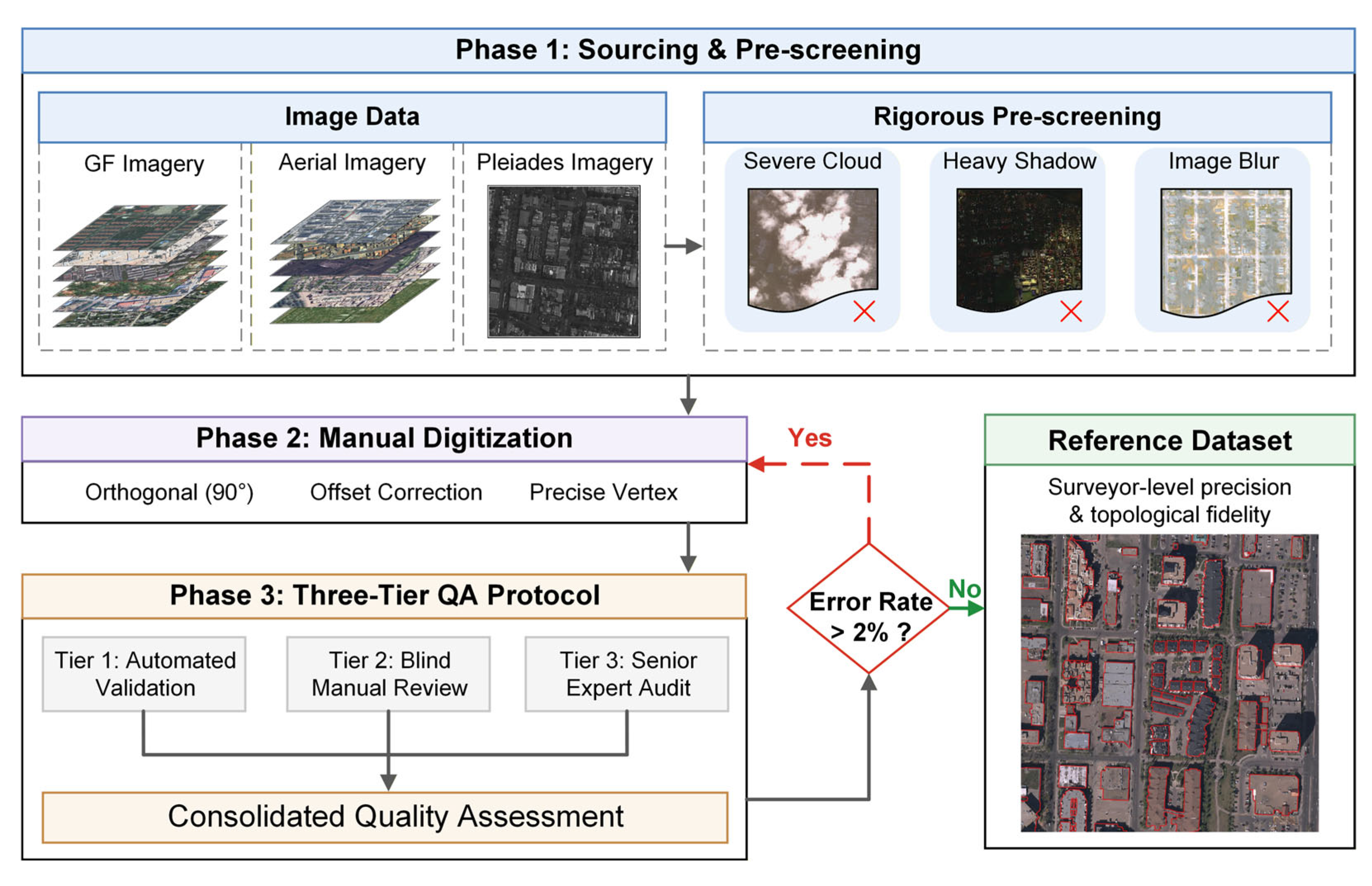
To construct a reliable reference dataset for quantitative evaluation, trained professional interpreters manually delineated building footprints following standardized annotation and quality-control procedures. This process produced a high-fidelity vector dataset comprising over 200,000 building footprints across 10 purposively selected cities across diverse global regions. The workflow included source-image screening, interpreter training and calibration, manual delineation under shared object and boundary rules, automated geometric and topological validation, blind peer review, and supervisory batch audit, as illustrated in Figure 1 and detailed below.

The source data comprised sub-meter GaoFen-02 (GF-02), GaoFen-07 (GF-07), Pleiades, and aerial imagery. Before delineation, each image was screened for cloud cover, heavy shadow, blur, and insufficient building visibility. Images in which building boundaries could not be interpreted reliably were not used. All interpreters received the same cartographic specifications and training before production.

During delineation, interpreters traced the visible outer boundary of each building and corrected identifiable roof-to-ground displacement. The specifications required consistent vertex placement, preservation of recognizable boundary detail, orthogonal regularization of rectilinear structures, and valid polygon topology. Adjacent structures were separated only when a visible boundary allowed them to be distinguished consistently. Small or partially occluded structures were included only when their outlines remained interpretable. The minimum mapping unit (MMU) was defined operationally by reliable boundary interpretation rather than by a single area threshold applied to all cities.

The digitized footprints underwent three quality-control stages. First, automated validation identified duplicate vertices, unclosed rings, self-intersections, unintended overlaps, and sliver polygons. Second, another interpreter independently checked building extent, local alignment, roof-offset correction, and topology against the source imagery. Nonconforming footprints were returned for redigitization. Third, senior supervisors inspected 20% of each submitted batch. The batch error rate was calculated as the proportion of inspected footprints containing at least one boundary, alignment, displacement, or topology error. A low error tolerance was necessary because the reference footprints supported object matching and boundary-based metrics, both of which are sensitive to delineation, alignment, and topology errors. Accordingly, batches with an error rate above 2% were corrected and reinspected before acceptance. The 2% cutoff served as an internal batch-rejection criterion for maintaining consistent production quality.

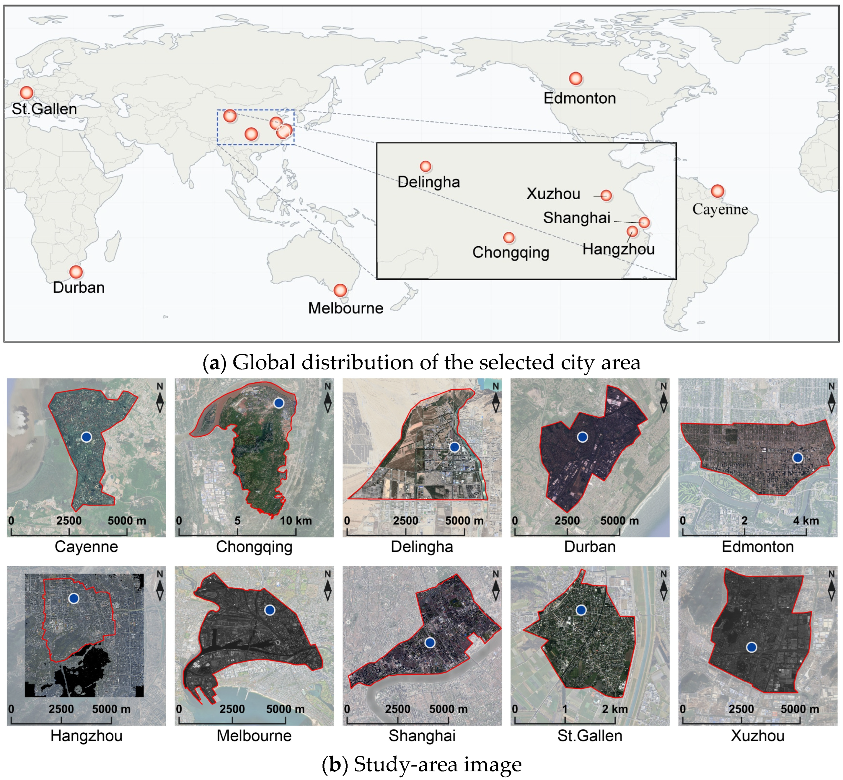
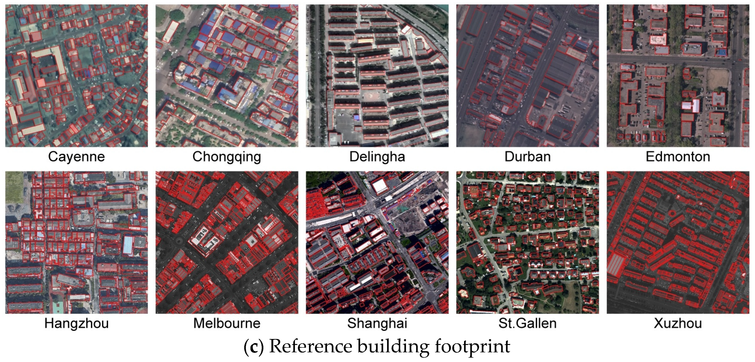
Following manual digitization and multi-stage quality assurance, the accepted reference labels were compiled into a building-footprint reference dataset comprising over 200,000 polygons across 10 cities. As shown in Figure 2, the study areas comprise Chongqing, Delingha, Durban, Edmonton, Cayenne, Hangzhou, Melbourne, Shanghai, St. Gallen, and Xuzhou. These cities were purposively selected to capture variation in geographical setting, urban morphology, architectural pattern, and topographic condition, thereby supporting evaluation across heterogeneous urban contexts.

The annotated areas were deliberately selected from established built-up zones rather than rapidly expanding urban fringes. To strictly mitigate temporal inconsistencies between our reference data and the varied timestamps of the evaluated products, we conducted visual cross-checks using historical Google Earth imagery spanning the respective temporal gaps. Any localized blocks exhibiting building construction or demolition were explicitly excluded from the reference extent. Consequently, the selected mature urban fabrics ensure highly stable building configurations, guaranteeing that the observed performance discrepancies stem from dataset quality rather than temporal mismatch.

Table 3. Characteristics of the selected areas and the corresponding reference data.

City Name	Country/Region	Urban Morphology Category	Study Area Size (km2)	Number of Reference Buildings	Temporal Baseline	Source Imagery	Number of Covered Datasets
Chongqing	China	Mountainous Megacity	81.4	15,997	2024-8	GF-07	7
Delingha	China	Arid Plateau Settlement	15.8	3971	2024-7	GF-07	4
Durban	South Africa	Coastal Hilly Urban Area	15.5	10,018	2024-10	GF-02	3
Edmonton	Canada	High-Latitude Grid Layout	8.3	8549	2024-8	Aerial	2
Cayenne	French Guiana	Tropical Forest Urban Fringe	10.0	10,061	2024-1	GF-07	3
Hangzhou	China	River Delta Megacity	11.0	21,585	2024-8	Aerial	7
Melbourne	Australia	Planned Low-Density Suburban	23.2	50,485	2024-4	Pleiades	3
Shanghai	China	High-Density Global Hub	16.4	35,817	2025-4	GF-07	9
St. Gallen	Switzerland	European Alpine Morphology	3.3	5280	2024-7	Aerial	2
Xuzhou	China	Industrial and Mining City	16.9	39,748	2024-9	GF-07	3

summarizes the characteristics of the ten selected urban regions and their corresponding manually annotated building footprint reference data, and the number of evaluated open-access building footprint datasets covering each city.

As shown in Table 3, the dataset contains in total 201,511 building instances, with the number of reference buildings varying substantially across cities, from 3971 in Delingha to 50,485 in Melbourne. Furthermore, the datasets demonstrate substantial heterogeneity across the study areas in both urban morphology and dataset coverage, which is essential for a balanced evaluation. The study areas span mountainous megacities, river delta hubs, arid plateau settlements, and alpine cities.

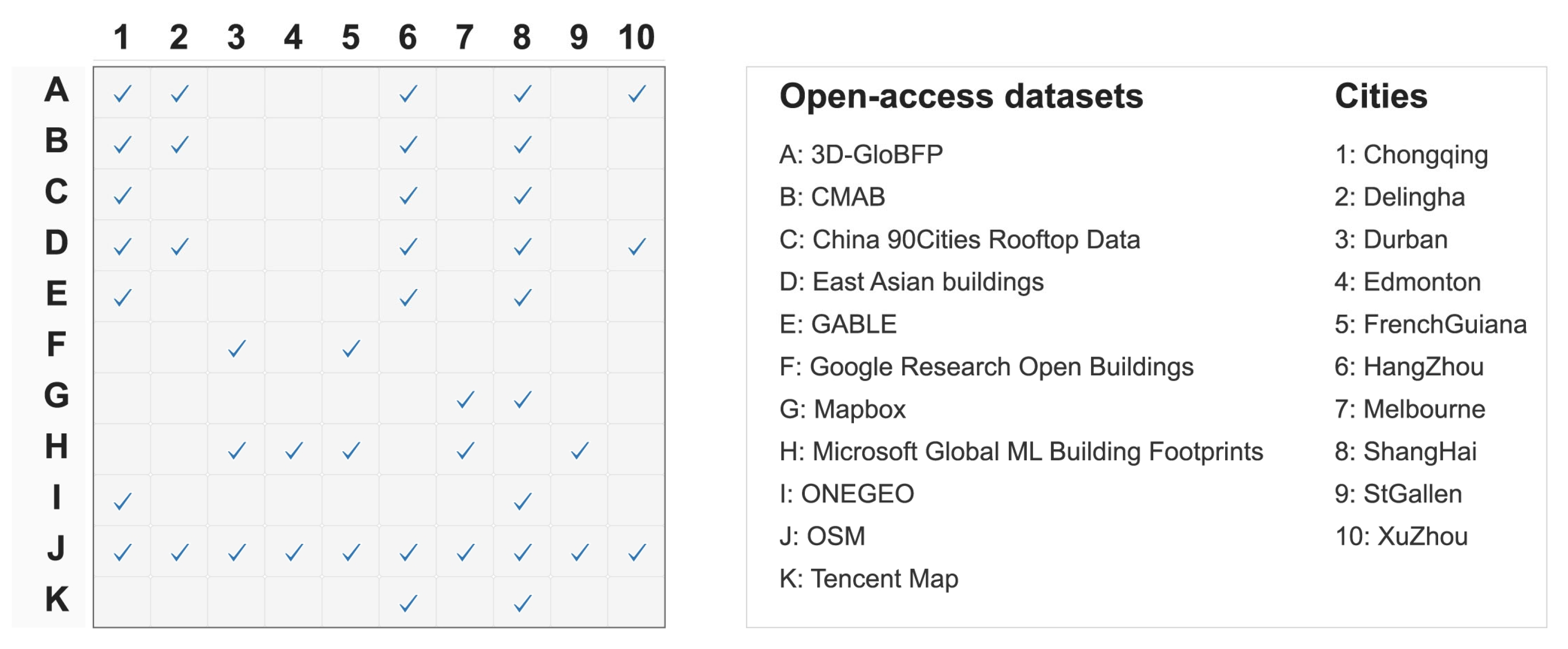
Figure 3 demonstrates the spatial intersection and data availability between the 11 evaluated open-access datasets and the 10 reference benchmark cities. While global-scale vector building datasets (i.e., OSM) exhibit ubiquitous coverage across nearly all target sites, regional or crowdsourced alternatives present localized availability or distinct spatial gaps, necessitating that subsequent metrics be aggregated only over valid spatial pairs.

3.2. Multi-Dimensional Evaluation Framework

To systematically evaluate the reliability of open-access building footprint datasets, we formulate a multi-dimensional assessment framework. The framework evaluates datasets across three complementary tiers: statistical consistency, object recovery and spatial fidelity, and morphology fidelity among matched building pairs. For each dataset $d$, the three dataset-level tier scores contributed equally to the overall score:

$$S_d={\displaystyle \frac{S_{1,d}+S_{2,d}+S_{3,d}}{3}}$$

(1)

where $S_d$ denotes the overall score of dataset $d$, whereas $S_{1,d}$, $S_{2,d}$, and $S_{3,d}$ denote its dataset-level scores for Tiers 1, 2, and 3, respectively. Each dataset-level tier score was obtained by averaging the corresponding city-level tier scores over all valid cities within the evaluated coverage. Missing city–dataset combinations were excluded from the averaging rather than assigned a score of zero.

Before equal-weight aggregation, the component indicators were converted to higher-is-better scores between 0 and 1 according to their original directions and scales. Indicators already expressed on a direction-aligned 0–1 scale were retained without further transformation. Bounded indicators with the opposite direction were reversed, whereas the remaining lower-is-better indicators were rescaled relative to the benchmark range using the following transformation:

$$s(x)={\displaystyle \frac{x_{\mathrm{m}\mathrm{a}\mathrm{x}}-x}{x_{\mathrm{m}\mathrm{a}\mathrm{x}}-x_{\mathrm{m}\mathrm{i}\mathrm{n}}}}$$

(2)

where $x_{\mathrm{m}\mathrm{i}\mathrm{n}}$ and $x_{\mathrm{m}\mathrm{a}\mathrm{x}}$ denote the benchmark-wide minimum and maximum values for the relevant indicator; the observations used to determine these bounds are specified in the corresponding tier subsection. All calculations retained full numerical precision, with rounding applied only to values presented in tables and figures. The resulting scores are therefore comparative summaries defined relative to the fixed benchmark population.

3.2.1. Statistical Consistency

Statistical consistency evaluates aggregate agreement in building count and footprint area. This tier is relevant for downstream applications such as urban population estimation, macroeconomic modeling, and regional building stock assessment, which rely on spatial capacity and structural density rather than precise boundary alignments [8,48,49].

To examine the spatial heterogeneity of statistical consistency, the study areas were further divided into local analysis grids. These grids were delineated primarily according to streets and natural spatial boundaries, rather than by a rigid regular grid, to better preserve the integrity of urban grids. All grids were manually inspected to ensure that no boundary intersected the ground-truth building footprints. For analysis grid $u$ in city $c$ and dataset $d$, signed count bias (${\Delta N}_{ucd}$) and area bias (${\Delta A}_{ucd}$) are calculated as [50]:

$$\begin{gathered} {\Delta N}_{ucd}={\displaystyle \frac{N_{OS,ucd}-N_{GT,ucd}}{N_{GT,ucd}}} \\ {\Delta A}_{ucd}={\displaystyle \frac{A_{OS,ucd}-A_{GT,ucd}}{A_{GT,ucd}}} \end{gathered}$$

(3)

where the subscripts $GT$ and $OS$ denote the reference and evaluated open-access data, respectively. $N_{OS,ucd}$ and $N_{GT,ucd}$ denote the numbers of evaluated and reference building objects, respectively, whereas $A_{OS,ucd}$ and $A_{GT,ucd}$ denote the corresponding total footprint areas within analysis grid $\mathrm{u}$. A value of zero indicates exact aggregate agreement, whereas negative and positive values indicate underestimation and overestimation, respectively.

Because deviations in either direction indicate disagreement, the signed biases were converted to nonnegative error magnitudes at the grid level:

$$\begin{gathered} E_{N,ucd}=\left|\Delta N_{ucd}\right| \\ {E}_{A,ucd}=\left|\Delta A_{ucd}\right| \end{gathered}$$

(4)

For each city–dataset combination, the absolute count and area biases were averaged separately across all valid analysis grids to obtain the corresponding city-level mean errors. Because the absolute values were taken before averaging, local overestimation and underestimation could not cancel each other. The original signed biases were retained for descriptive maps and distributional analyses.

The city-level mean count and area errors were then converted to higher-is-better scores using Equation (2), yielding $s_{N,cd}$ and $s_{A,cd}$, respectively. For each indicator, the minimum and maximum in Equation (2) were determined separately from the pooled grid-level absolute biases across all valid analysis grids and all city–dataset combinations in the benchmark. The same benchmark-wide bounds were applied to every city–dataset combination, ensuring comparability across cities and datasets within the fixed benchmark. The two component scores were assigned equal weights to obtain the Tier 1 score for city c and dataset d:

$$S_{1,cd}={\displaystyle \frac{s_{N,cd}+s_{A,cd}}{2}}$$

(5)

Here, $S_{1,cd}$ is the city-level Tier 1 score; averaging it over all valid cities for dataset $d$ yields $S_{1,d}$, the dataset-level Tier 1 score used in Equation (1).

3.2.2. Object Recovery and Spatial Fidelity

This tier evaluates both object recovery over the complete building inventory and spatial fidelity at the full-set and matched-object levels. This metric group is critical for precision-dependent applications such as autonomous navigation, cadastral mapping, and disaster emergency response [51,52,53].

For building-level evaluation, spatial entity matching was performed to establish one-to-one correspondences between individual reference and evaluated footprints. Candidate pairs were first identified by spatial intersection, and pairwise pixel-based IoU was then used to establish one-to-one matches, with 0.30 adopted as the primary threshold. Split and merged configurations were not treated as one-to-many or many-to-one-correspondences. Under the one-to-one matching rule, unmatched evaluated-footprints arising from split cases were counted as false positives, whereas unmatched-reference footprints associated with-merged cases were counted as false negatives, and were therefore penalized through-Object F1. Sensitivity to this choice is examined in Section 4.2.4. To better account for both matched and unmatched objects, object $F1$ was calculated as:

$$F{1}_{\mathrm{o}\mathrm{b}\mathrm{j},cd}={\displaystyle \frac{2{TP}_{cd}}{2{TP}_{cd}+{FP}_{cd}+{FN}_{cd}}}$$

(6)

where $T{P}_{cd}$ denotes the number of true positives (accepted one-to-one matches), and ${FP}_{\mathrm{c}\mathrm{d}}$ and ${FN}_{\mathrm{c}\mathrm{d}}$ denote the numbers of false positives (evaluated footprints without an accepted reference match) and false negatives (reference footprints without an accepted evaluated match), respectively. Object $F1$ summarizes object recovery under the specified matching protocol by penalizing both unmatched reference footprints and unmatched evaluated footprints.

Spatial overlap was evaluated at two levels on a common raster grid. City-level IoU measured full-set agreement between the unions of all reference and evaluated footprints, whereas mean object-level IoU summarized pairwise agreement across accepted one-to-one matches. Both were calculated as follows [54]:

$$\begin{gathered} Io{U}_{city,cd}={\displaystyle \frac{\left|C_{cd}^{GT}\cap C_{cd}^{OS}\right|}{\left|C_{cd}^{GT}\cup C_{cd}^{OS}\right|}} \\ Io{U}_{obj,cd}={\displaystyle \frac{1}{{TP}_{cd}}}{\displaystyle \sum _{k=1}^{{TP}_{cd}}}{\displaystyle \frac{\left|B_k^{GT}\cap B_k^{OS}\right|}{\left|B_k^{GT}\cup B_k^{OS}\right|}} \end{gathered}$$

(7)

where $C_{cd}^{GT}$ and $C_{cd}^{OS}$ denote the pixel sets collectively occupied by all reference and evaluated footprints, respectively, in city $c$ for dataset $d$; $B_k^{GT}$ and $B_k^{OS}$ denote the pixel sets occupied by the two footprints in the $k$-th accepted pair; $\left|·\right|$ denotes the number of pixels.

Beyond area overlap, positional disagreement was quantified using the RMSE between the centroids of accepted building pairs in city $c$ for dataset $d$ [50]:

$$RMS{E}_{cd}=\sqrt{{\displaystyle \frac{1}{{TP}_{cd}}}{\displaystyle \sum _{k=1}^{{TP}_{cd}}}\left[{\left(X_k^{GT}-X_k^{OS}\right)}^2+{\left(Y_k^{GT}-Y_k^{OS}\right)}^2\right]}$$

(8)

where $\left(X_k^{GT},Y_k^{GT}\right)$ and $\left(X_k^{OS},Y_k^{OS}\right)$ denote the centroid coordinates of the reference and evaluated footprints, respectively, in the $k$-th accepted pair.

Object F1, city-level IoU, and mean object-level IoU are higher-is-better indicators bounded between 0 and 1 and were used directly in the aggregation. The mean object-level IoU was obtained by averaging Equation (7) over all accepted matches in each city–dataset combination. Centroid RMSE is lower-is-better and was converted to a higher-is-better score $s_{\mathrm{R}\mathrm{M}\mathrm{S}\mathrm{E},cd}$ using Equation (2). Its minimum and maximum were determined from the centroid RMSE values of all valid city–dataset combinations in the benchmark, and the same bounds were applied throughout. The four component scores were assigned equal weights to obtain the Tier 2 score for city $c$ and dataset $d$:

$$S_{2,cd}={\displaystyle \frac{F{1}_{\mathrm{o}\mathrm{b}\mathrm{j},cd}+{IoU}_{\mathrm{c}\mathrm{i}\mathrm{t}\mathrm{y},cd}+{IoU}_{\mathrm{o}\mathrm{b}\mathrm{j},cd}+s_{\mathrm{R}\mathrm{M}\mathrm{S}\mathrm{E},cd}}{4}}$$

(9)

The score in Equation (9) is defined at the city–dataset level; averaging it over all valid cities for dataset $d$ yields the dataset-level Tier 2 score used in Equation (1).

3.2.3. Morphology Fidelity of Matched Building Pairs

This tier evaluates morphology fidelity among building pairs for which an accepted one-to-one correspondence has been established. These structural attributes are indispensable for emerging domains such as high-fidelity 3D urban reconstruction, digital twin modeling, and microclimate simulations [49,55,56].

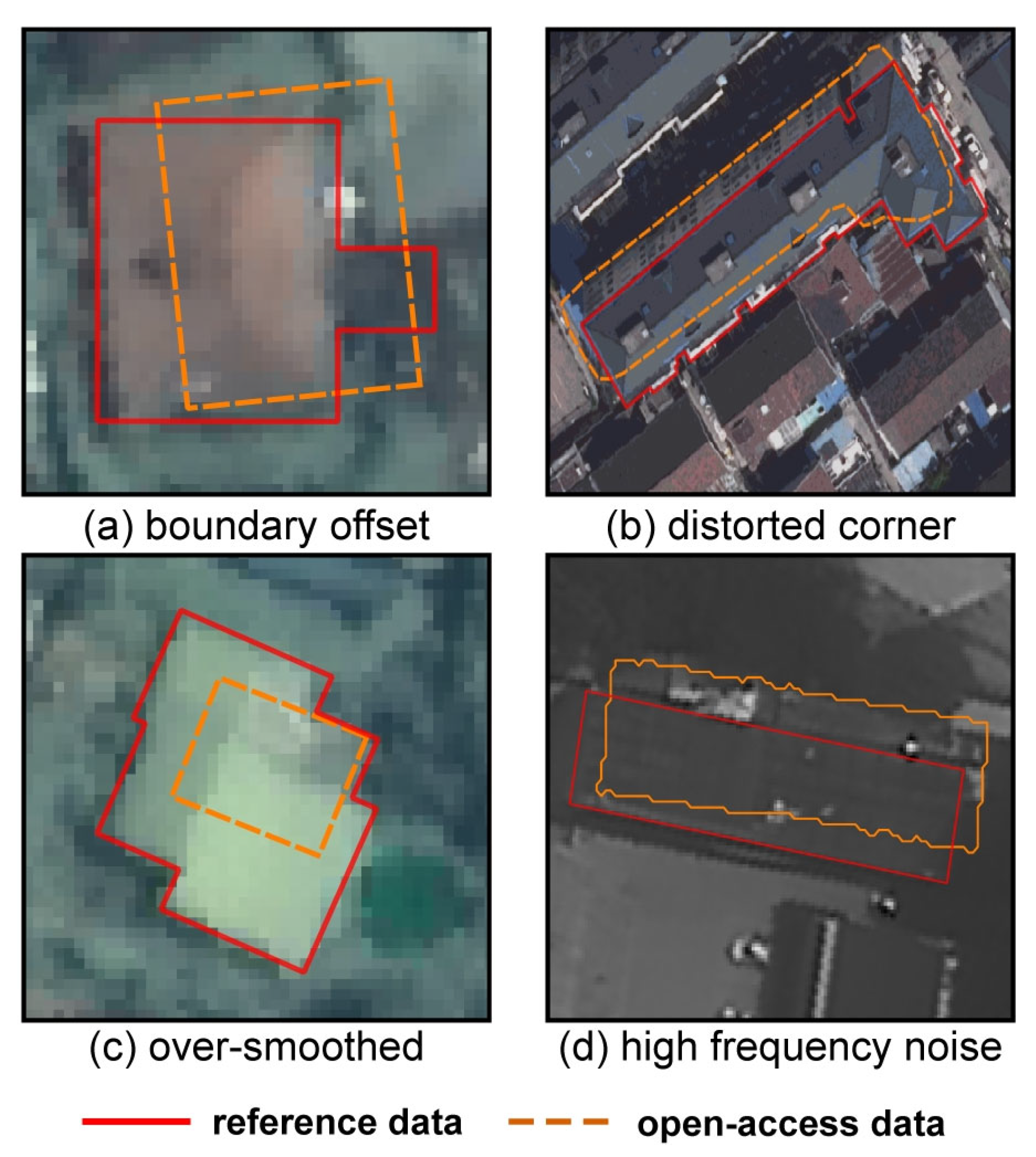
In practical building footprint extraction, morphological degradation commonly occurs in several forms, including boundary displacement, angular-structure distortion, compactness inconsistency, and high-frequency contour noise. Figure 4 schematically illustrates these typical degradation patterns. Based on these characteristics, we employ four complementary descriptors to quantify complementary aspects of matched-pair morphology fidelity: PoLiS distance, turning function distance, compactness deviation, and Fourier descriptors [18,38,57,58].

As illustrated in Figure 4, boundary displacement and contour deformation between the two footprints in a matched polygon pair, denoted by $A$ and $B$, were quantified using the PoLiS distance, a symmetric measure based on the average shortest distances from the vertices of each polygon to the boundary of the other [38]:

$$PoLiS\left(A,B\right)={\displaystyle \frac{1}{2q}}\sum _{a_j\in A}\underset{b\in \partial B}{\min }\Vert a_j-b\Vert +{\displaystyle \frac{1}{2r}}\sum _{b_k\in B}\underset{a\in \partial A}{\min }\Vert b_k-a\Vert$$

(10)

where $a_j$ and $b_k$ are vertices of $A$ and $B$; $q$ and $r$ are their corresponding vertex counts; and $\partial A$ and $\partial B$ are their continuous boundaries.

Complementing the boundary distance, the turning function distance quantifies morphological similarity independent of spatial translation or scale [18]. It evaluates the cumulative angle of the tangent ($\Theta$) as a function of the normalized arc length ($l$) along the polygon boundary, effectively capturing the preservation of rigid, orthogonal architectural corners:

$$d_{\mathrm{T}\mathrm{F}}\left(A,B\right)=\underset{\theta ,t}{\min }{\int }_0^1|{\Theta }_A\left(\lambda \right)-{\Theta }_B\left(\lambda +\mathrm{t}\right)+\theta ||\mathrm{d}\lambda$$

(11)

where $\mathrm{t}$ denotes a cyclic shift in the boundary starting point, with $\lambda +\mathrm{t}$ interpreted cyclically, and $\Theta$ denotes relative rotation.

Additionally, we evaluate the global structural complexity and fragmentation of building footprints using the compactness deviation ($\Delta C$) [59]:

$$\Delta C=\left|{\displaystyle \frac{4\pi \times {Area}_{OS}}{{\left({Perimeter}_{OS}\right)}^2}}-{\displaystyle \frac{4\pi \times {Area}_{GT}}{{\left({Perimeter}_{GT}\right)}^2}}\right|$$

(12)

where $Are{a}_D$ and $Perimete{r}_D$ denote the planar area and boundary length of footprint for $D\in \{OS,GT\}$; $\Delta C$ is the absolute difference between their compactness values. This metric determines if the automated extraction overly smoothed or artificially fragmented the true morphology. Finally, Fourier descriptors are utilized to transform the spatial coordinate sequence of a closed boundary into the frequency domain. By comparing the low- and high-frequency coefficients, Fourier descriptors effectively assess global contour similarity and the retention of fine-grained architectural details [57,58].

For each valid city–dataset combination, PoLiS distance, turning function distance, and Fourier-descriptor distance were averaged separately across all accepted matched pairs to obtain city-level mean distances. Each mean distance was converted to a higher-is-better score using Equation (2), with metric-specific benchmark-wide bounds derived from all accepted matched-pair values and applied throughout. Compactness required no benchmark-range rescaling: for each matched pair, its compactness score was calculated directly as $1-\Delta C$, and these pair-level scores were averaged to obtain the city-level compactness score. The four component scores were assigned equal weights to obtain the Tier 3 score for city $c$ and dataset $d$:

$$S_{3,cd}={\displaystyle \frac{s_{\mathrm{P}\mathrm{o}\mathrm{L}\mathrm{i}\mathrm{S},cd}+s_{\mathrm{T}\mathrm{F},cd}+s_{\mathrm{c}\mathrm{o}\mathrm{m}\mathrm{p}\mathrm{a}\mathrm{c}\mathrm{t}\mathrm{n}\mathrm{e}\mathrm{s}\mathrm{s},cd}+s_{\mathrm{F}\mathrm{D},cd}}{4}}$$

(13)

where $s_{\mathrm{P}\mathrm{o}\mathrm{L}\mathrm{i}\mathrm{S},cd}$, $s_{\mathrm{T}\mathrm{F},cd}$, $s_{\mathrm{c}\mathrm{o}\mathrm{m}\mathrm{p}\mathrm{a}\mathrm{c}\mathrm{t}\mathrm{n}\mathrm{e}\mathrm{s}\mathrm{s},cd}$, and $s_{\mathrm{F}\mathrm{D},cd}$ denote the direction-aligned city-level scores for PoLiS distance, turning function distance, compactness, and Fourier-descriptor distance, respectively. The score in Equation (13) is defined at the city–dataset level; averaging it over all valid cities for dataset d yields the dataset-level Tier 3 score used in Equation (1). Tier 3 is conditional on the accepted one-to-one matches and does not independently quantify unmatched reference or evaluated objects.

3.3. Data Standardization and Evaluation Implementation

Before metric computation, each evaluated dataset and the corresponding reference footprints were transformed to a common, locally appropriate projected coordinate reference system. This avoided mixing native coordinate systems and ensured that distance and area metrics were calculated in consistent linear units.

The evaluation framework was implemented using Python (v3.9) in the Visual Studio Code (v2026) environment. The calculations were conducted on a workstation running Windows 11 X64, equipped with a 13th Generation Intel Core i5 CPU (2.50 GHz) and 16 GB of RAM. The open-access vector datasets were obtained from official GitHub (accessed on 30 June 2026) repositories and data platforms through programmatic extraction or direct downloads.

Furthermore, we developed an open-source Skill package, available at https://github.com/Tykuinn/building-footprint-eval (accessed on 16 August 2026), to facilitate practical reuse of the benchmark framework. The Skill organizes the detailed accuracy reports and dataset metadata generated in this study into a structured knowledge module. By referencing these embedded evaluation results, it supports interactive dataset recommendation by matching dataset strengths to user-defined selection criteria and application scenarios.

4. Results and Discussion

4.1. Overall Scoring Results

We report coverage-conditional product summaries by averaging each tier score across the cities covered by the corresponding dataset. The overall score is calculated as the equal-weight mean of the three tier scores.

Table 4. Coverage-conditional tier and overall scores for the 11 evaluated datasets.

Dataset	Number of Covered Cities	Tier 1	Tier 2	Tier 3	Overall Score
3D-GloBFP	5	0.595	0.435	0.696	0.576
CMAB	4	0.523	0.343	0.620	0.495
China-90C	3	0.609	0.453	0.495	0.519
East Asian buildings	5	0.631	0.431	0.694	0.585
GABLE	3	0.853	0.502	0.759	0.705
GOB	2	0.641	0.561	0.803	0.668
Mapbox	2	0.610	0.423	0.667	0.567
MBF	5	0.751	0.587	0.709	0.682
ONEGEO	2	0.419	0.388	0.684	0.497
OSM	10	0.438	0.444	0.715	0.532
Tencent Map	2	0.573	0.468	0.698	0.580

* Tiers 1–3 denote Statistical Consistency, Object Recovery and Spatial Fidelity, and Matched-Pair Morphology Fidelity, respectively. Tier 3 is calculated only for accepted one-to-one matches. Boldface and underlining indicate the largest and second-largest values, respectively, within each score column.

reports the number of covered cities together with the resulting tier and overall scores. The corresponding city-level component scores and aggregation inputs are provided in Appendix A 

Table A1. Component scores for Tier 1: Statistical Consistency.

Dataset	Count-Error Score	Area-Error Score	Tier 1: Statistical Consistency
3D-GloBFP	0.477	0.713	0.595
CMAB	0.325	0.721	0.523
China-90C	0.421	0.796	0.609
East Asian Buildings	0.531	0.731	0.631
GABLE	0.721	0.986	0.853
GOB	0.330	0.952	0.641
Mapbox	0.365	0.855	0.610
MBF	0.666	0.836	0.751
ONEGEO	0.293	0.544	0.419
OSM	0.371	0.505	0.438
Tencent Map	0.339	0.807	0.573

* The count- and area-error scores were derived from the two-sided magnitudes of the corresponding signed biases. The Tier 1 score is the equal-weight arithmetic mean of the two component scores. Calculations used full-precision values; the values shown here were rounded to six decimal places.

,

Table A2. Component scores for Tier 2: Object Recovery and Spatial Fidelity.

Dataset	Object F1	City-Level IoU Score	Object-Level IoU Score	Centroid-RMSE Score	Tier 2: Object Recovery and Spatial Fidelity
3D-GloBFP	0.197	0.633	0.405	0.505	0.435
CMAB	0.138	0.438	0.325	0.470	0.343
China-90c	0.232	0.593	0.465	0.523	0.453
East Asian Buildings	0.205	0.643	0.378	0.500	0.431
GABLE	0.261	0.737	0.454	0.557	0.502
GOB	0.410	0.791	0.547	0.496	0.561
Mapbox	0.138	0.620	0.480	0.455	0.423
MBF	0.439	0.756	0.583	0.571	0.587
ONEGEO	0.136	0.594	0.291	0.530	0.388
OSM	0.238	0.619	0.371	0.550	0.444
Tencent Map	0.214	0.684	0.455	0.519	0.468

* Object F1 was calculated at an IoU matching threshold of 0.30. The Tier 2 score is the equal-weight arithmetic mean of object F1, the centroid-RMSE score, the object-level IoU score, and the city-level IoU score. None of the four components was multiplied by object F1.

and

Table A3. Component scores for Tier 3: Matched-Pair Morphology Fidelity.

Dataset	PoLiS Score	Turning-Function Score	Fourier-Descriptor Score	Compactness Score	Tier 3: Matched-Pair Morphology Fidelity
3D-GloBFP	0.595	0.943	0.341	0.906	0.696
CMAB	0.388	0.952	0.261	0.878	0.620
China-90C	0.593	0.348	0.232	0.809	0.495
East Asian Buildings	0.611	0.973	0.288	0.902	0.694
GABLE	0.720	0.961	0.459	0.894	0.759
GOB	0.711	0.992	0.561	0.948	0.803
Mapbox	0.513	0.958	0.307	0.889	0.667
MBF	0.671	0.788	0.467	0.911	0.709
ONEGEO	0.517	0.940	0.386	0.891	0.684
OSM	0.550	0.876	0.528	0.907	0.715
Tencent Map	0.564	0.932	0.420	0.874	0.698

* All four morphology descriptors were calculated only for accepted one-to-one matches and normalized as lower-is-better indicators. The Tier 3 score is their equal-weight arithmetic. It therefore characterizes morphology fidelity conditional on successful matching and should be interpreted together with the object-recovery statistics reported in Table A2.

.

As shown in Table 4, the three tiers exhibited distinct score distributions under the defined scoring configuration. Tier 1 scores ranged from 0.419 to 0.853, Tier 2 scores from 0.343 to 0.587, and Tier 3 scores from 0.495 to 0.803. Tier 2 remained below Tier 3 for every product, whereas Tier 3 exceeded Tier 1 for eight of the eleven products. China-90C, GABLE, and MBF were the exceptions, with Tier 1 scores of 0.609, 0.853, and 0.751 and Tier 3 scores of 0.495, 0.759, and 0.709, respectively. Because the tiers contain different indicators and normalization procedures, their numerical levels should not be interpreted as direct evidence that one quality attribute is inherently stronger than another. Instead, the separation reflects differences in the properties assessed by each tier.

Aggregate agreement was not consistently accompanied by object recovery and spatial fidelity. For example, Mapbox, East Asian buildings, and GABLE produced Tier 1 scores of 0.610, 0.631, and 0.853, respectively, but their Tier 2 scores were 0.423, 0.431, and 0.502. GOB showed a smaller separation, with scores of 0.641 and 0.561 for Tier 1 and Tier 2, respectively. These profiles indicate that agreement in aggregate building count and footprint area can coexist with omissions, commissions, positional displacement, or incomplete object correspondence. Tier 1 indicators alone are therefore insufficient to characterize object-level dataset quality.

Tier 2 and Tier 3 also captured different aspects of performance. Across the products, Tier 3 exceeded Tier 2 by 0.042–0.296. GOB, East Asian buildings, and CMAB, for example, produced Tier 3 scores of 0.803, 0.694, and 0.620, compared with Tier 2 scores of 0.561, 0.431, and 0.343. This separation is consistent with their different evaluation scopes. Tier 2 incorporates object recovery, regional overlap, matched-object overlap, and centroid displacement, whereas Tier 3 describes morphology fidelity only among accepted one-to-one matches. Consequently, well-matched objects may retain their contour characteristics even when full-set object recovery or spatial correspondence remains limited. Tier 3 should therefore be interpreted jointly with Tier 2 rather than as an independent measure of complete-set quality.

Similar overall scores also concealed different tier profiles. GABLE and GOB produced overall scores of 0.705 and 0.668, respectively. GABLE’s summary contained a larger Tier 1 contribution, whereas the GOB summary contained larger Tier 2 and Tier 3 contributions within its two-city subset. A comparable contrast occurred between China-90C and ONEGEO, whose overall scores were 0.519 and 0.497. China-90C had a larger Tier 1 score, while ONEGEO had a larger Tier 3 score. In addition, 3D-GloBFP, East Asian buildings, Mapbox, and Tencent Map fell within a narrow overall-score interval of 0.567–0.585 despite being evaluated over different numbers and combinations of cities. The overall score thus provides a concise synthesis but cannot substitute for inspection of the contributing tier scores.

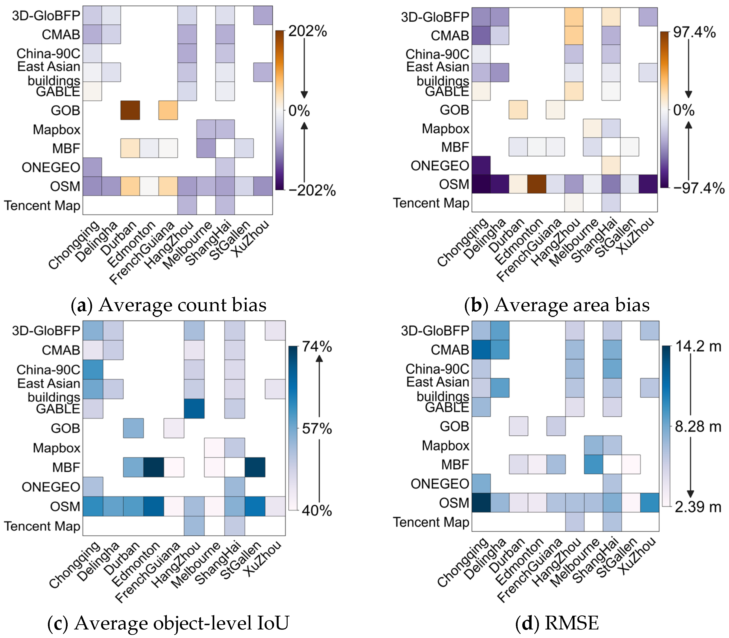
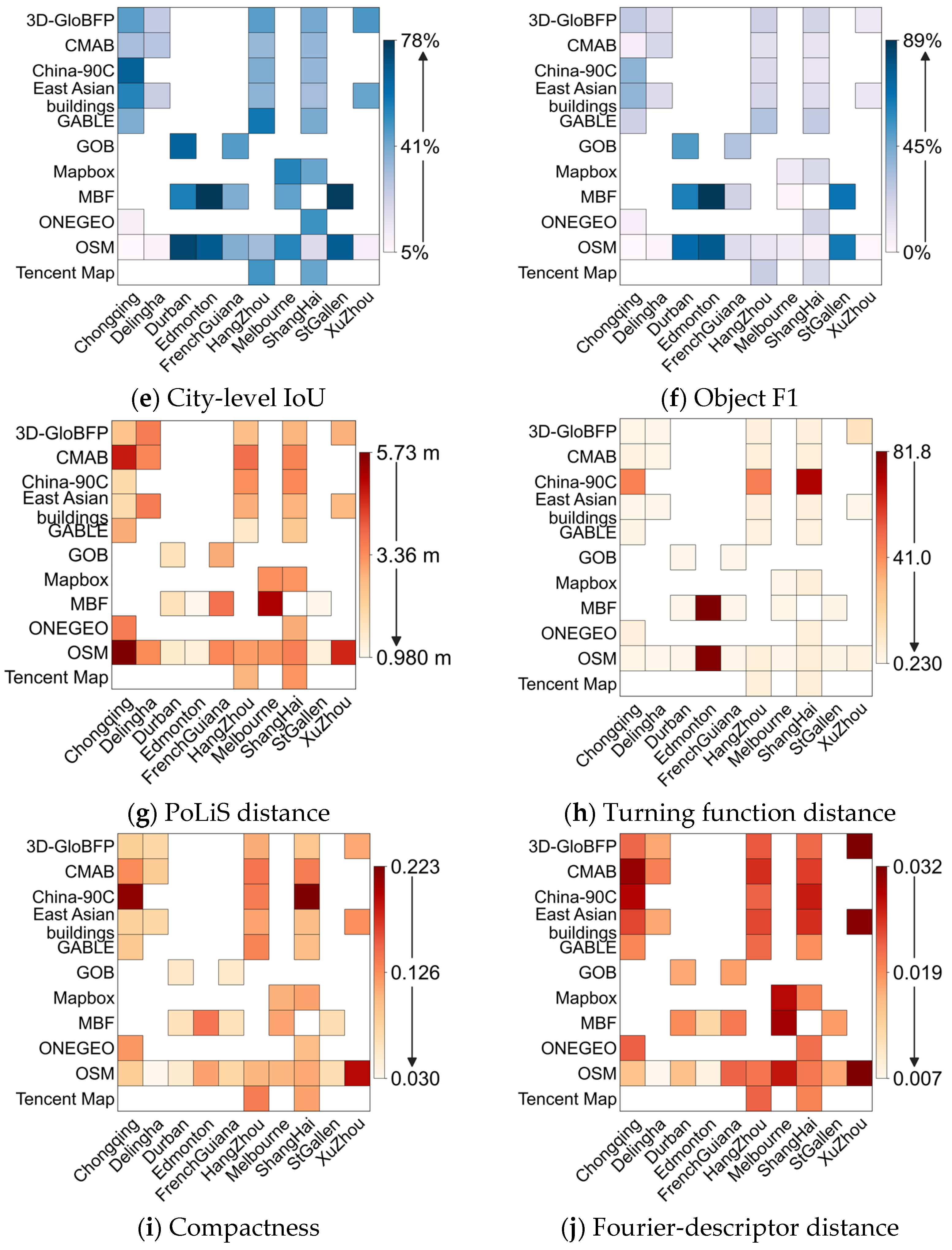
Figure 5 presents city–dataset heatmaps for the nine evaluation components. In each panel, rows represent the evaluated datasets and columns represent the ten study cities. Arrows adjacent to the color bars indicate the direction of improving performance; for the signed count and area biases, the arrows point toward the optimal value of zero.

As shown in Figure 5, a more detailed view of city-level variation reveals how these performance patterns manifest across different urban contexts. Overall, MBF and GABLE maintain relatively stable performance across multiple cities, with achieving consistently strong overall scores, whereas GOB shows more pronounced advantages in spatial accuracy and morphology-sensitive applications, with particularly high Tier 2 and Tier 3 scores. In contrast, several middle-performing datasets exhibit clear dimension-specific strengths, suggesting that their suitability depends strongly on the target application and local urban morphology. Together, these observations indicate that dataset performance is shaped by the interplay among statistical consistency, spatial alignment, and morphological fidelity, rather than by any single metric alone.

4.2. Tier-Specific Performance Patterns

4.2.1. Statistical Bias Patterns

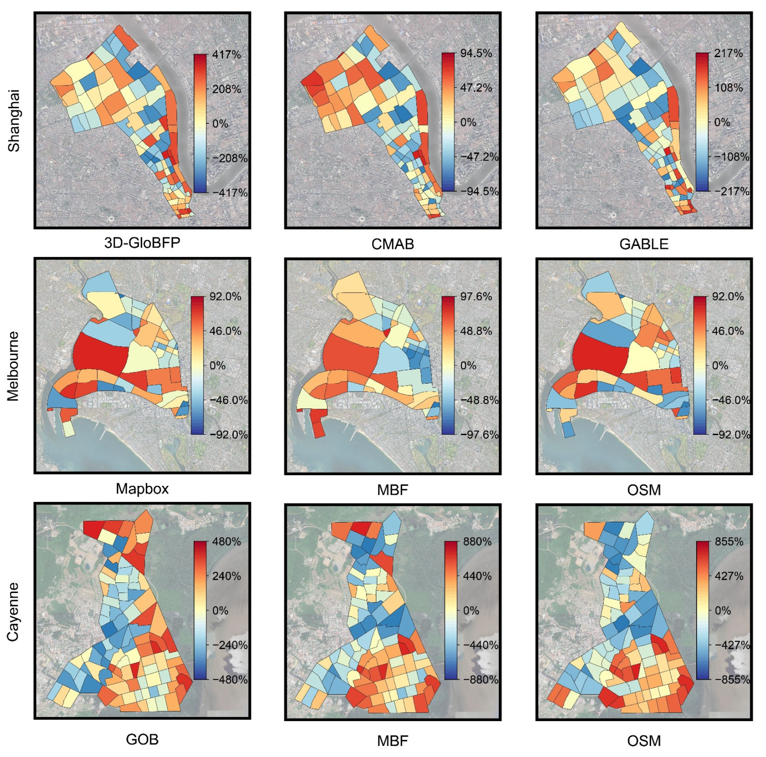
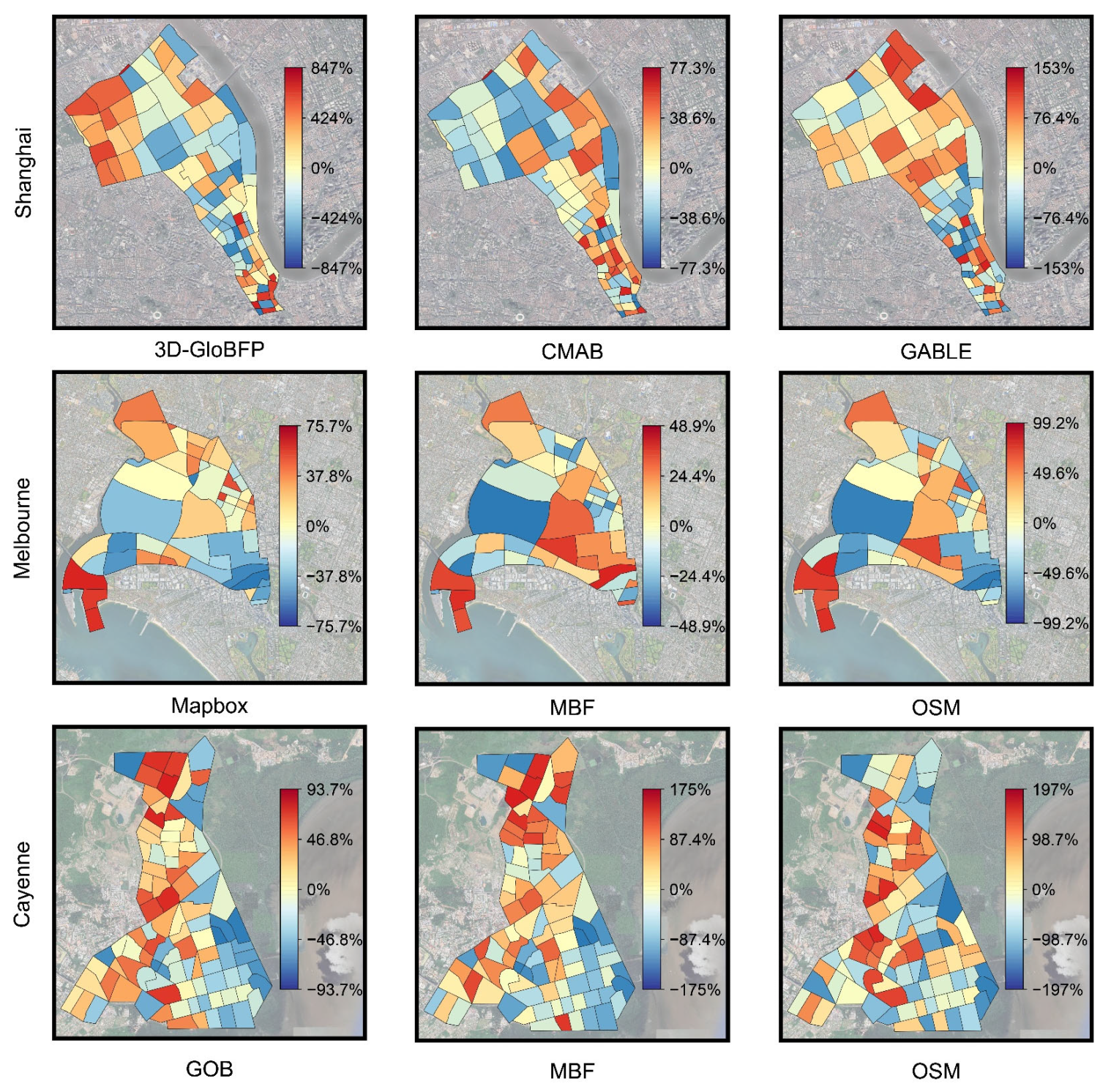
While the overall scores establish a macro-level baseline, understanding the root causes of these performance variations requires dissecting the fundamental statistical consistency of the extracted features. Figure 6 and Figure 7 present grid-level maps of count bias and area change across representative city–dataset pairs. Grid cells are colored by the count and area bias respectively.

As shown in Figure 6 and Figure 7, statistical inconsistency is not uniformly distributed across the study areas but is spatially clustered within specific urban fabrics. Count bias is more pronounced in dense or morphologically complex grids, where adjacent buildings are more likely to be merged or omitted. In contrast, area change exhibits a partly different spatial pattern, indicating that errors in building quantity and errors in areal representation are not always coupled. Some grids with substantial count underestimation still show moderate area deviation, suggesting that merged polygons may preserve built-up extent while losing object-level separability. These patterns provide direct evidence that statistical consistency is shaped by both dataset generation strategy and local urban morphology.

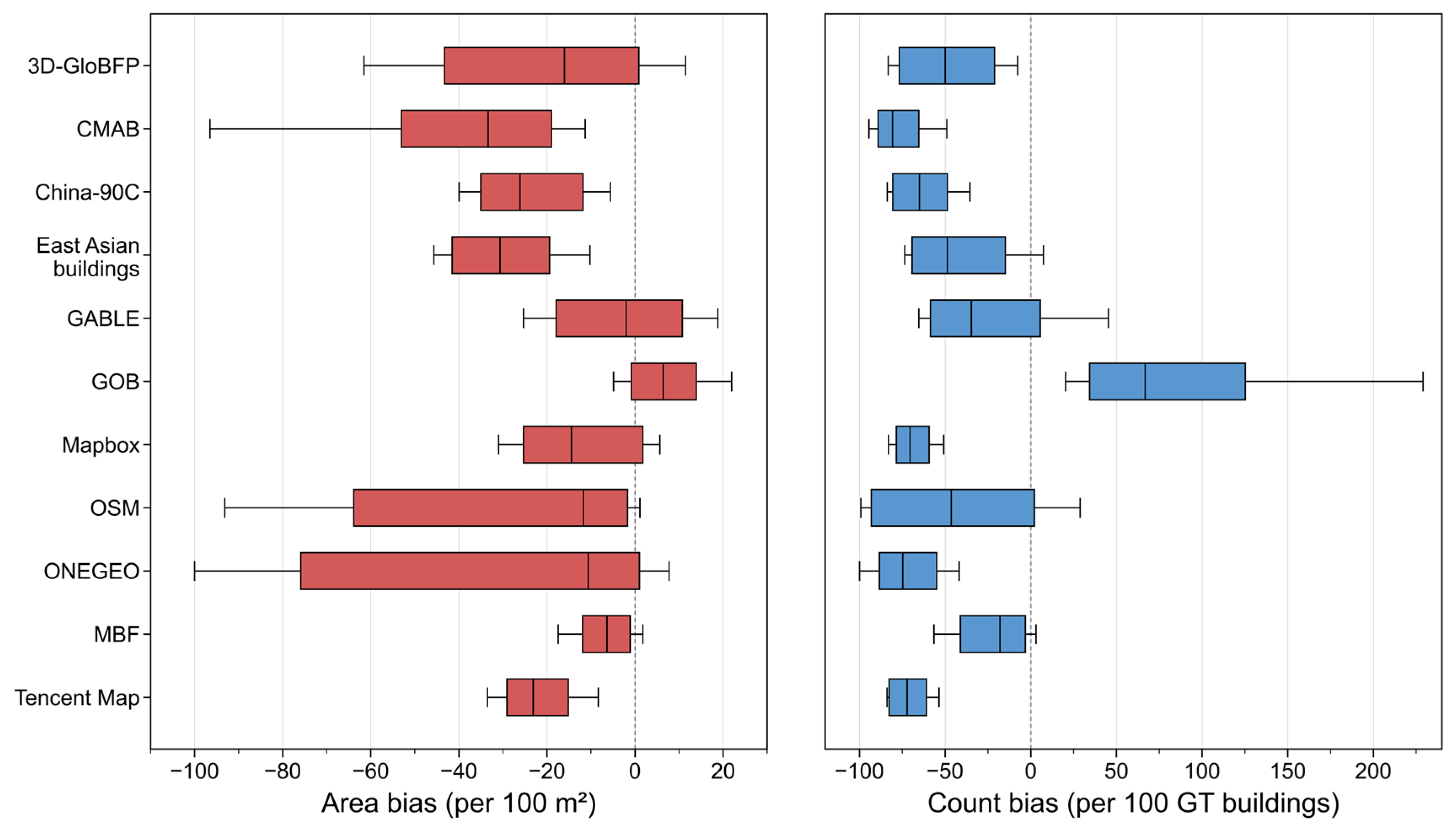
Figure 8 summarizes the grid-level distributions of building count bias and area change for each evaluated dataset. The box represents the interquartile range, while the central line indicates the average value. It represents the relative count bias per 100 reference buildings and the areal change per 100 m² of reference building area.

Figure 8 reveals systematic discrepancies in both building count estimation and areal representation across datasets. For building count, most datasets exhibit negative biases, indicating that omission and under-segmentation remain common issues in open-access building footprint products. This pattern is particularly evident in densely built-up areas, where multiple adjacent buildings are frequently merged into a single polygon, thereby reducing the apparent number of detected building instances. In contrast, GABLE and MBF show comparatively smaller count biases, suggesting stronger building-level separability and more stable segmentation behavior in moderately dense urban contexts.

GOB presents a different pattern, with a tendency toward higher building counts in several grid cells. This overestimation is likely associated with finer-grained segmentation of contiguous or semi-connected structures, where built-up blocks represented as single buildings in the reference data may be decomposed into multiple smaller footprint entities. This behavior improves local structural detail in some cases but may also introduce inconsistency when building boundaries are ambiguous.

The area-change boxplots further indicate that low count bias does not necessarily correspond to stable areal representation. MBF and Tencent Map exhibit relatively compact distributions, implying lower grid-level variability and more consistent areal estimation across spatial samples. By contrast, OSM and ONEGEO show broader interquartile ranges and more pronounced dispersion, reflecting spatially uneven data quality. For OSM, this variability is consistent with heterogeneous crowdsourced mapping practices, whereas for ONEGEO it is likely related to multi-source data fusion and uneven sample coverage. Overall, it demonstrates that statistical inconsistency is not only expressed as systematic overestimation or underestimation, but also as substantial spatial dispersion across local grid units.

4.2.2. Object Recovery and Spatial Agreement Patterns

The Tier 2 analysis considers full-set areal agreement, object recovery, and positional fidelity among accepted matches. As shown in Figure 5e, city-level IoU varies substantially across both cities and datasets, indicating that spatial agreement is strongly context dependent. MBF generally achieves higher city-level IoU values across multiple cities, suggesting strong areal agreement with the reference footprints. GOB also shows high overlap where coverage is available, although its limited spatial coverage constrains broader comparison. In contrast, datasets such as CMAB, ONEGEO, and OSM exhibit more variable or lower city-level IoU values, reflecting less stable spatial coverage or stronger regional dependence.

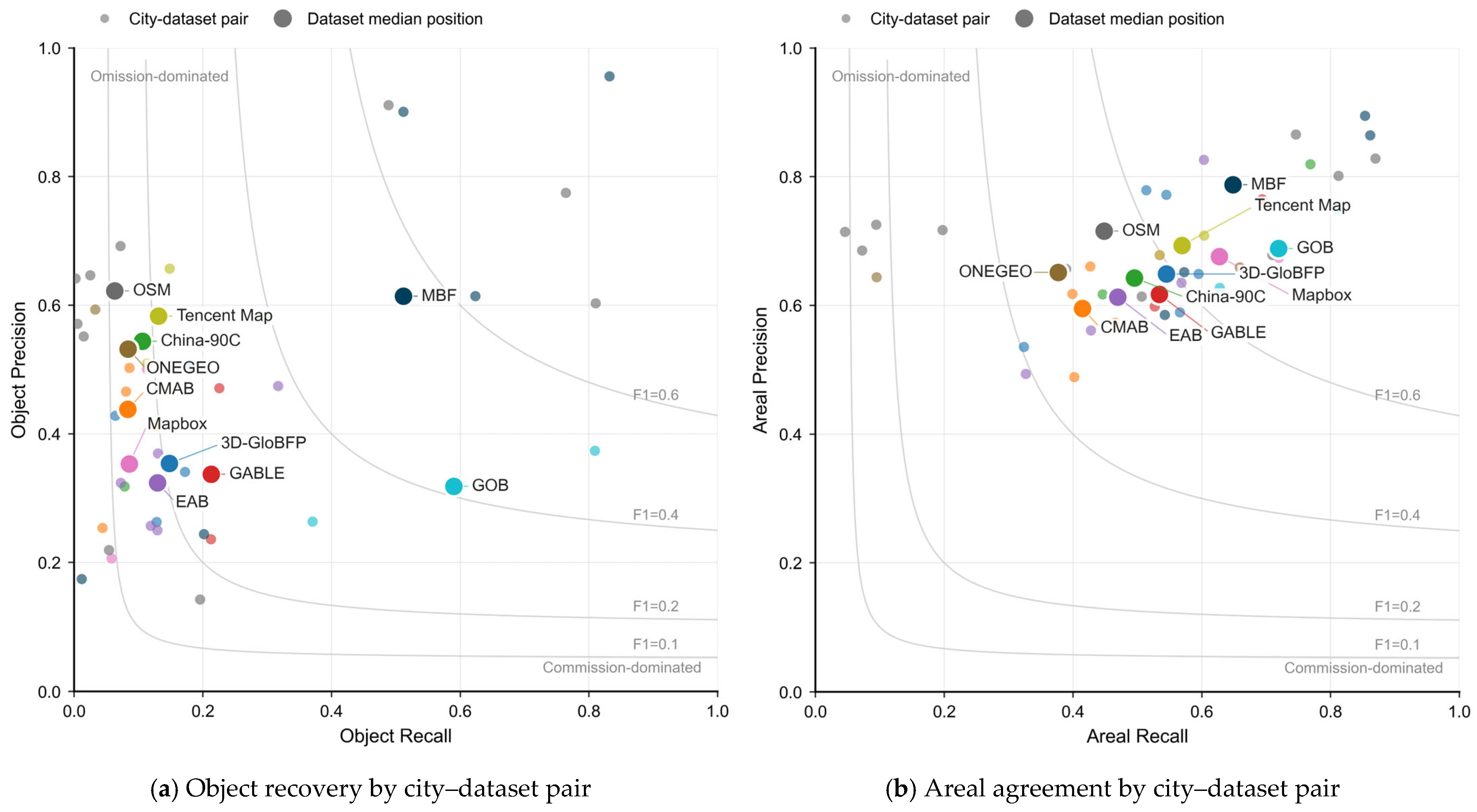
Figure 9 further characterizes object recovery by jointly plotting object recall and object precision. Positions toward the upper-right indicate that a dataset recovers a larger proportion of reference buildings while limiting unmatched predictions. The upper-left region instead indicates omission-dominated behavior, whereas the lower-right region indicates commission-dominated behavior. The light iso-F1 curves provide a supplementary reference for interpreting the balance between the two components.

The object-level precision–recall plot reveals distinct recovery patterns across datasets. MBF showed median recall and precision of approximately 0.51 and 0.61, respectively, with both omission and commission contributing to unmatched objects. GOB showed higher median recall (0.59) but lower precision (0.32), indicating broader object recovery accompanied by more unmatched predictions within its two-city subset. In contrast, OSM had a median precision of 0.62 but a recall of only 0.06, indicating an omission-dominated pattern. CMAB, Mapbox, ONEGEO, and several regional products were likewise concentrated in the low-recall region, although their precision varied.

The areal precision–recall plot provides a complementary complete-set assessment derived from the same intersection, false-positive, and false-negative areas used to calculate City-IoU. MBF had median areal recall and precision of approximately 0.65 and 0.79, while the corresponding values for GOB were 0.72 and 0.69. Several datasets with low object recall nevertheless retained moderate areal recall. For example, Mapbox increased from an object recall of 0.09 to an areal recall of 0.63, while OSM increased from 0.06 to 0.45. This contrast indicates that substantial footprint area may overlap the reference even when individual buildings are not recovered as distinct one-to-one objects. Such patterns are consistent with differences in object partitioning, including merged or split footprints, rather than boundary displacement alone.

The dispersion of city–dataset observations in both plots further shows that recovery performance varies across geographic contexts. The object-level plot identifies whether omission or commission limits instance recovery, whereas the areal plot characterizes the corresponding imbalance in total footprint coverage. These measures should therefore be interpreted jointly with City-IoU and matched-pair geometry metrics. Because the datasets cover different city subsets, the observed positions are coverage-conditional summaries rather than controlled cross-dataset rankings.

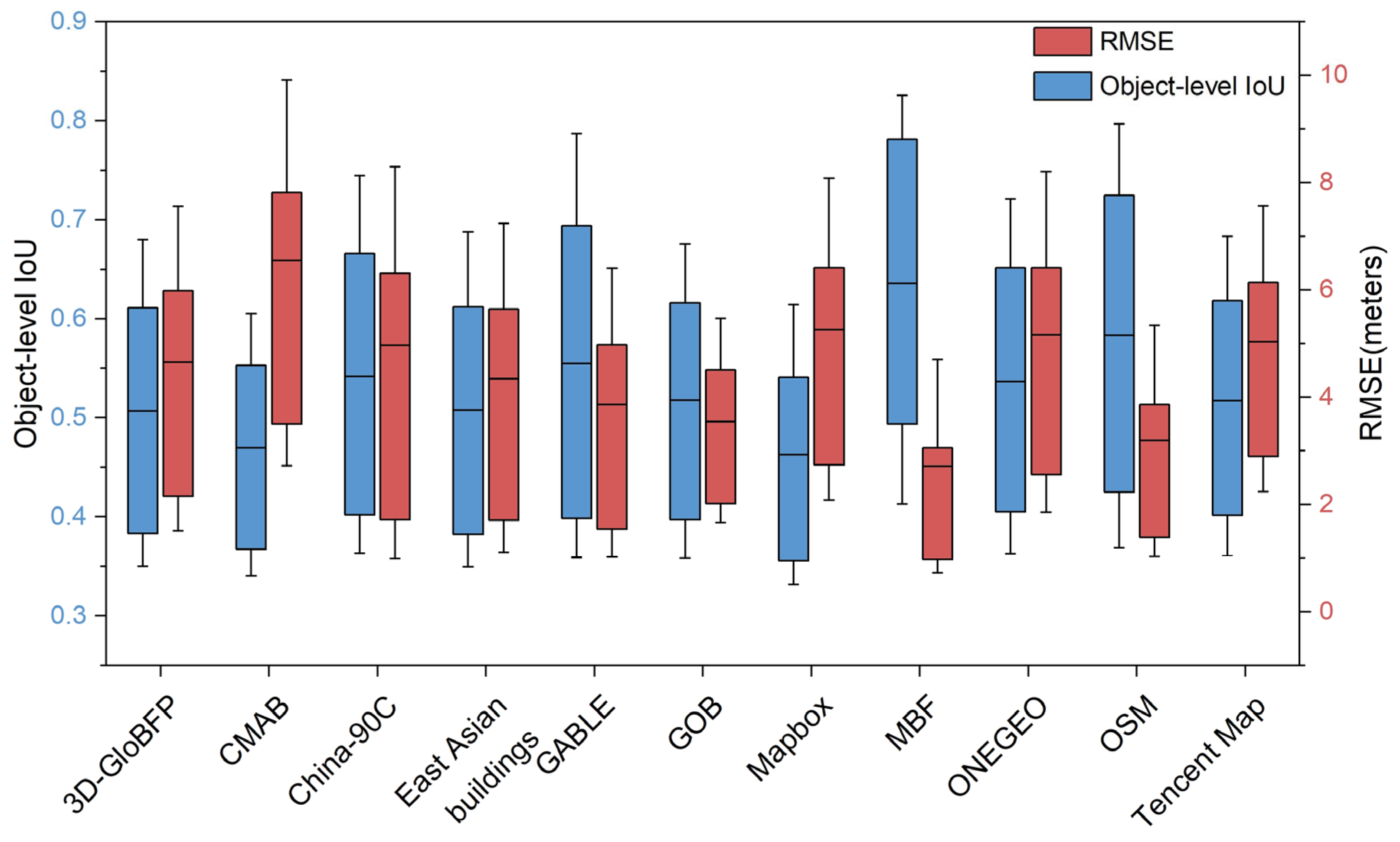
Figure 10 presents box plots illustrating the distribution of RMSE and IoU across ten open-access datasets. The box represents the interquartile range, while the central line indicates the mean value, providing a robust summary of central tendency and dispersion for each evaluation metric.

As shown in Figure 10, the object-level IoU distribution centers around approximately 0.5, while the RMSE values are generally concentrated around 5 m. This pattern suggests that, within the benchmark, current open-access building footprint products achieve a moderate level of geometric overlap with the reference data, while still exhibiting non-negligible positional deviations. Such behavior is likely attributable to inherent limitations in large-scale automated extraction pipelines, including mixed-resolution training imagery, inconsistent vectorization standards, and the difficulty of accurately delineating building boundaries in dense or irregular urban environments.

Among all datasets, MBF exhibits a notably higher average object-level IoU and a substantially lower RMSE compared to other datasets, indicating superior geometric alignment and improved positional accuracy relative to the ground truth. This performance advantage is likely driven by higher-quality training data, more robust model generalization, and more refined post-processing strategies that enhance both footprint completeness and boundary precision.

In contrast, the CMAB dataset shows a significantly higher RMSE than the other datasets, suggesting larger positional discrepancies in footprint localization. This may be attributed to variations in data acquisition sources, heterogeneous annotation standards, or less strict geometric correction procedures during post-processing, which can collectively lead to systematic spatial misalignment and increased positional error.

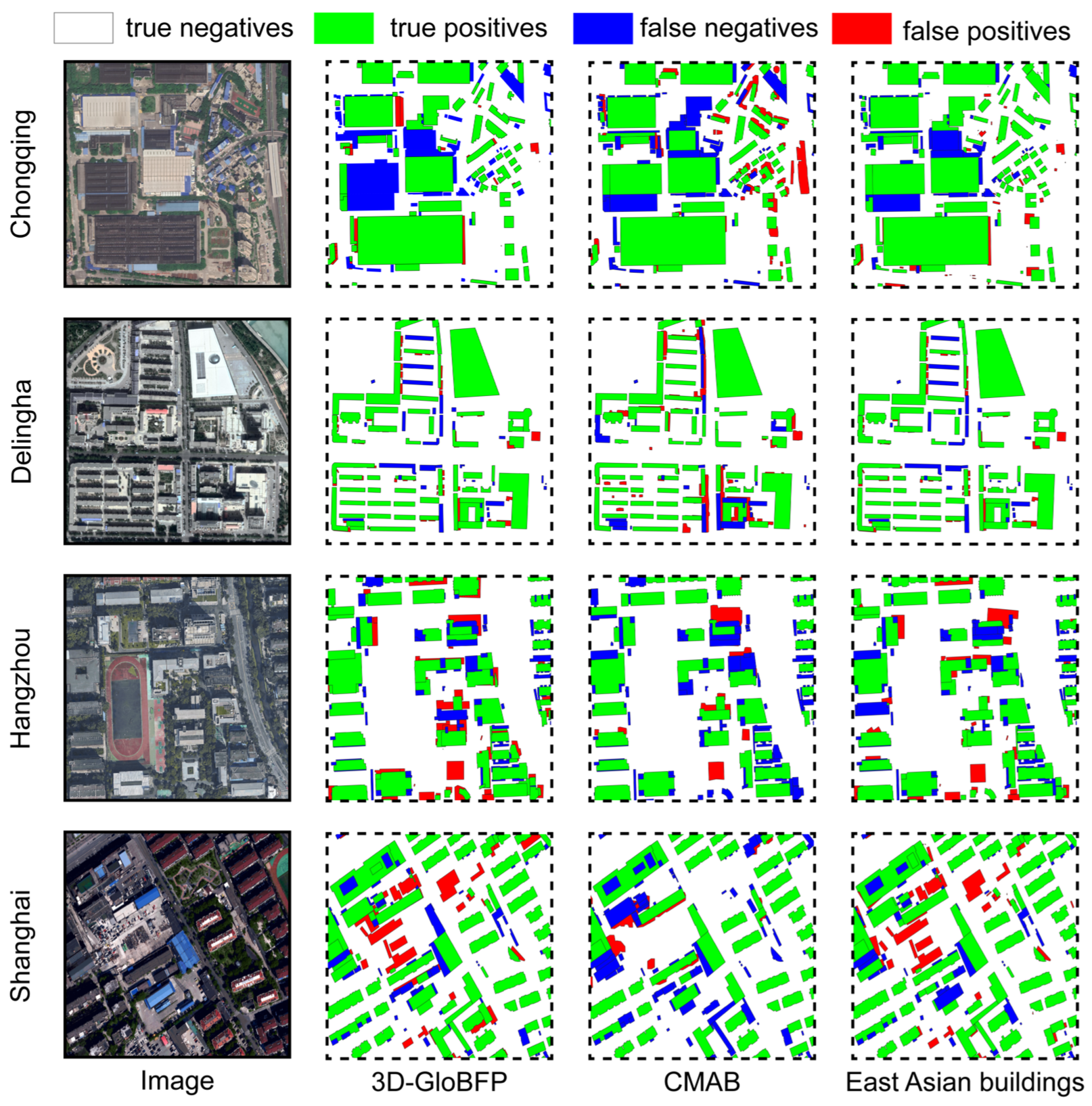
Figure 11 illustrates the spatial comparison outcomes between the evaluated datasets and the ground truth across representative urban regions.

As observed in Figure 11, the CMAB dataset exhibits a visibly higher frequency of commission and omission errors across the four selected cities compared to 3D-GloBFP and East Asian Buildings. This visual evidence intuitively corroborates the significantly higher RMSE observed for CMAB in the prior statistical analysis. Furthermore, the spatial matching maps for 3D-GloBFP and East Asian Buildings are nearly identical in Delingha and Shanghai, and show only marginal discrepancies in Hangzhou and Chongqing. This striking visual consistency unveils a finding not explicitly detailed earlier: it directly explains their highly similar object-level IoU and RMSE distributions presented in Figure 10, indicating comparable spatial extraction logic and boundary alignment capabilities between these two datasets.

4.2.3. Morphology Score Distributions Among Matched Pairs

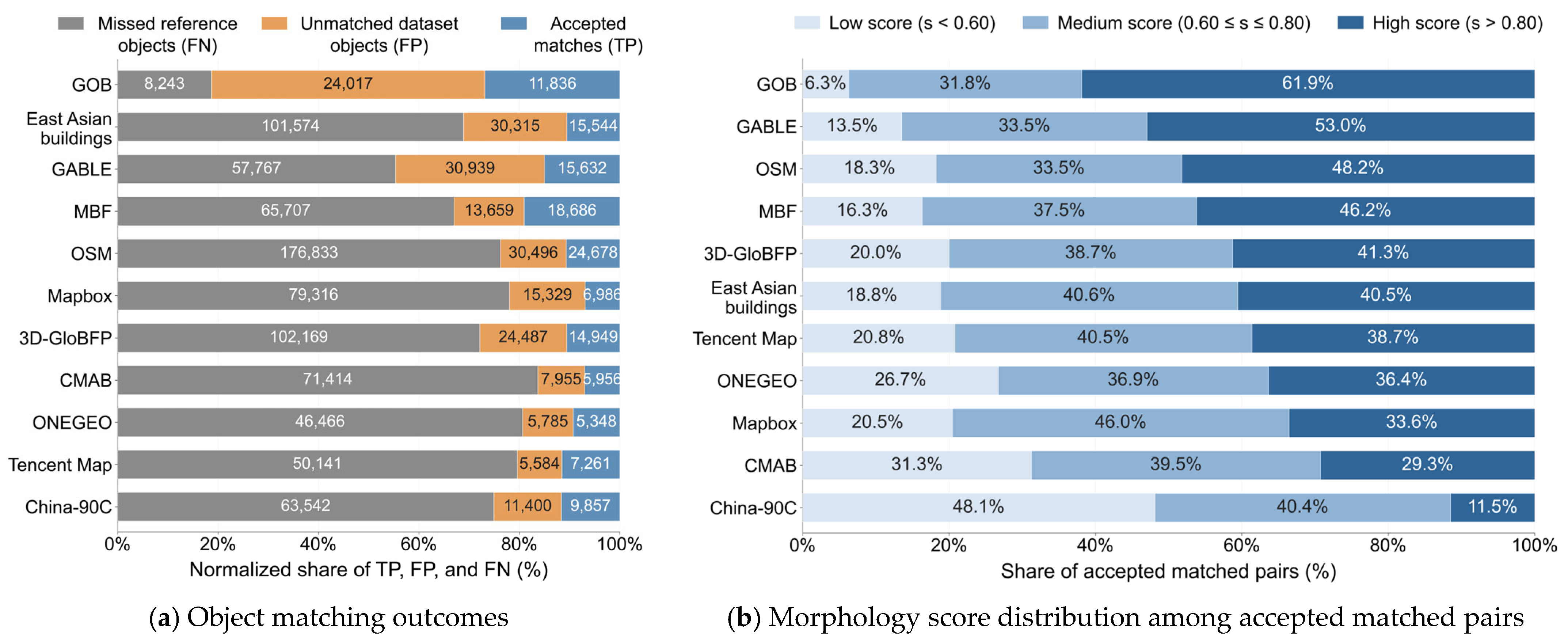
To characterize shape fidelity across open-access building footprint datasets, we examined the distribution of footprint instances according to their similarity scores relative to the reference data. To place this conditional analysis in the context of overall object recovery, Figure 12 jointly summarizes object-matching outcomes and morphology-score distributions across datasets. Figure 12a presents the relative composition and pooled counts of TP, FP, and FN, whereas Figure 12b reports the proportions of accepted matched pairs with scores below 0.60, between 0.60 and 0.80, and above 0.80. Higher score bands indicate closer agreement with the reference footprints, but these thresholds serve as descriptive cutoffs for cross-dataset comparison rather than absolute quality standards.

Figure 12a shows that FN constitutes the largest outcome category for every dataset except GOB, indicating that omission is the main limitation of object recovery. GOB has the largest relative TP share, but FP accounts for more than half of its pooled outcomes. OSM records the largest absolute TP count (24,678), yet its much larger FN count (176,833) leaves accepted matches as a relatively small proportion.

Among accepted matches, Figure 12b shows that GOB has the largest share of scores above 0.80 (61.9%), followed by GABLE (53.0%), OSM (48.2%), and MBF (46.2%). China-90C presents the opposite pattern, with 48.1% of scores below 0.60 and only 11.5% above 0.80. The remaining datasets occupy intermediate positions, with substantial proportions concentrated between 0.60 and 0.80.

Read together, the two panels show that object recovery and conditional shape fidelity do not necessarily vary in parallel. GOB combines the largest upper-score share with the highest relative TP share, but also contains many unmatched dataset objects. OSM exhibits relatively strong shape fidelity among accepted matches despite being dominated by unmatched reference objects. The morphology-score distribution should therefore be interpreted as conditional on successful matching rather than as a measure of overall dataset completeness.

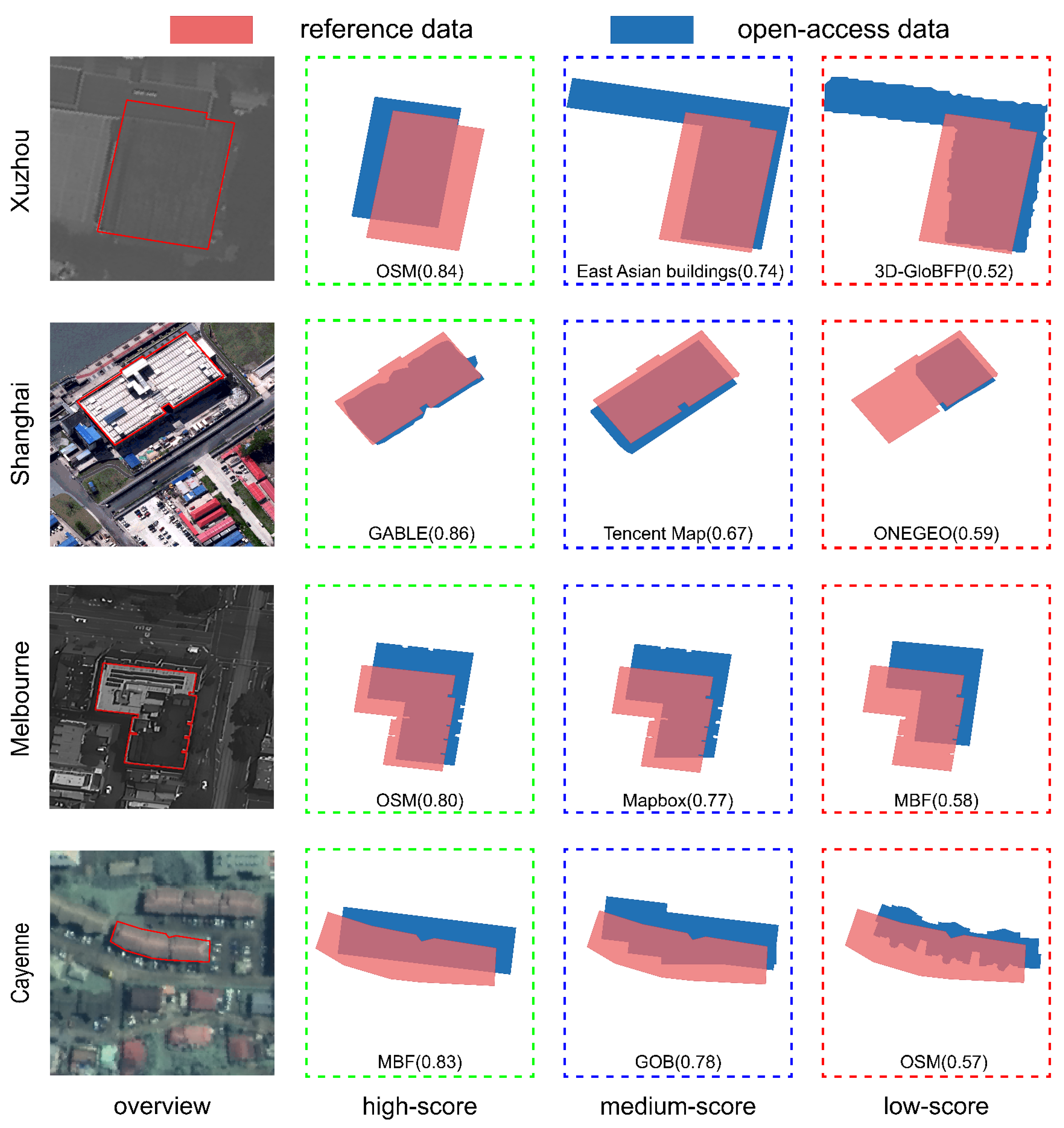
To illustrate the shape differences represented by these score bands, Figure 13 presents representative matched pairs from the three intervals. The first column identifies the sample locations, while the remaining columns overlay the reference and evaluated footprints, accompanied by their dataset names and normalized scores.

Figure 13 demonstrates that the proposed score categories correspond well to distinct levels of geometric fidelity. High-score footprints closely match the ground truth, exhibiting accurate boundary delineation with minimal omission or redundant details. Medium-score footprints generally preserve the overall building geometry but show moderate deviations, typically reflected by partial loss of fine-scale details or locally redundant structures. In contrast, low-score footprints exhibit pronounced geometric distortions, including oversimplified outlines, irregular polygon boundaries, jagged edges, and excessive redundant structures.

Representative examples illustrate these characteristic error patterns. For instance, the Mapbox dataset in Melbourne, along with the ONEGEO and Tencent Map datasets in Shanghai, exhibits varying degrees of omission of fine-scale structural details. In contrast, the East Asian Buildings and GOB datasets introduce redundant geometric details in Xuzhou and Cayenne, respectively. More severe degradation is observed in low-score footprints, including oversimplified outlines (MBF in Melbourne), excessive redundant structures (OSM in Cayenne), and jagged edges (3D-GloBFP in Xuzhou).

Overall, the decline in footprint score is associated with increasingly severe geometric representation errors. These errors primarily arise from boundary simplification, over-segmentation, and boundary irregularities introduced during polygon generation or post-processing, ultimately reducing the geometric similarity between predicted footprints and the reference annotations.

4.2.4. Sensitivity to the Object-Matching IoU Threshold

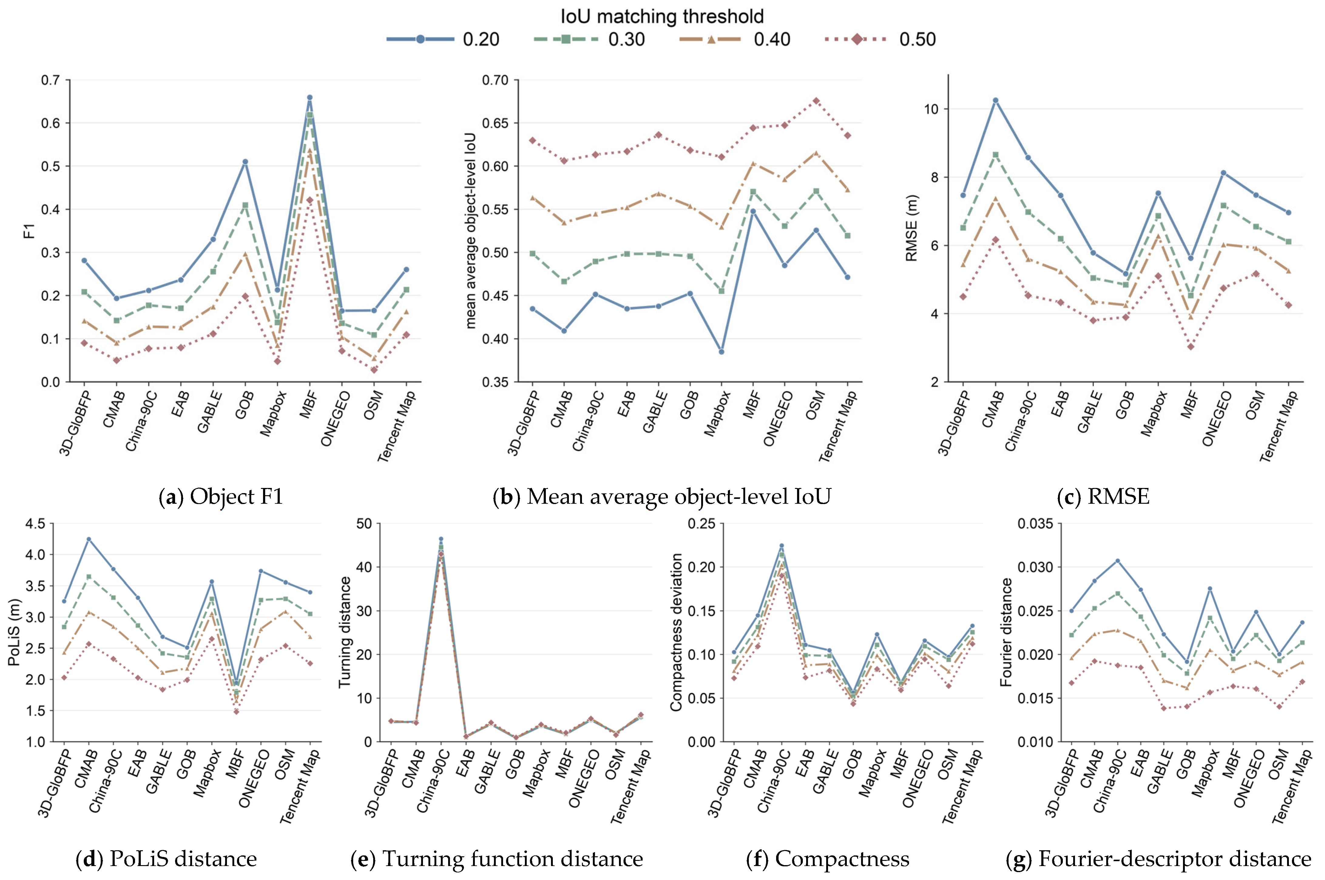
As the IoU matching threshold directly determines which object pairs are accepted, its choice may influence both object-recovery performance and morphological metrics derived from matched pairs. We therefore examined the threshold sensitivity of the metrics underlying Tier 2 and Tier 3. Four thresholds, $\mathrm{I}\mathrm{o}\mathrm{U}=0.20, 0.30, 0.40, \mathrm{a}\mathrm{n}\mathrm{d} 0.50$, were evaluated. For each dataset and threshold, the plotted value represents the median of its city-level metric values across the cities covered by that dataset as Figure 14 illustrated.

For Tier 2, increasing the matching threshold produced the expected trade-off between object recovery and conditional fidelity (Figure 14a–c). Object F1 decreased consistently, whereas mean object-level IoU increased and centroid RMSE declined. The main product contrasts nevertheless remained recognizable: MBF retained comparatively strong object recovery and low RMSE, while OSM and ONEGEO showed relatively high conditional IoU despite lower F1. This contrast confirms that object recovery and matched-pair fidelity capture different aspects of dataset performance.

The Tier 3 metrics exhibited similar threshold-dependent changes (Figure 14d–g). PoLiS distance, compactness deviation, and Fourier-descriptor distance generally decreased as the threshold increased because stricter matching retained more closely overlapping pairs. Turning-function distance showed no uniform trend, indicating that greater overlap does not necessarily correspond to stronger angular-structure agreement. Persistent product characteristics also remained visible: MBF, GABLE, and GOB generally had smaller PoLiS distances, whereas China-90C retained a distinct morphology profile, particularly in turning-function distance and compactness deviation.

Despite these changes in metric magnitude, the broad product-level patterns remained stable. Relative to the primary threshold of 0.30, seven metrics produced Spearman correlations of 0.827–1.000 across the alternative settings; only Fourier-descriptor distance declined to 0.773 at the threshold of 0.50. Stricter matching narrowed some between-product differences but did not materially alter the comparative conclusions. The evaluation is therefore reasonably robust to the matching threshold within the tested range, while remaining conditional on each product’s city coverage.

4.3. Dataset Adoption Suggestions

In practical applications, dataset selection is constrained by both data quality and geographic availability. For studies requiring broad and consistent spatial coverage, particularly those spanning multiple countries or regions, OSM remains a practical baseline because of its extensive availability. Although OSM does not consistently outperform other products and shows relatively weak statistical consistency, it provides moderate object recovery and spatial fidelity together with comparatively strong morphology fidelity, and can therefore serve as a useful general-purpose or fallback dataset where higher-performing regional products are unavailable. Nevertheless, its quality varies substantially among cities, reflecting the heterogeneous nature of crowdsourced mapping. Therefore, when applications require higher reliability or finer spatial detail, OSM and other open-access products should be supplemented by local validation, manual correction, or authoritative mapping data where available.

For applications primarily concerned with statistical consistency, such as large-scale building-stock characterization, population estimation, or comparative urban analysis, existing open-access datasets can provide a useful approximation of broad spatial patterns. However, the systematic underestimation of building count and area observed in this study indicates that these products should not be interpreted as direct substitutes for authoritative statistics. Their reliability also decreases as the analytical scale becomes finer. At regional or city scales, substantial spatial heterogeneity may emerge, particularly in dense and morphologically complex urban areas where omission and building aggregation are more frequent. Within the evaluated coverage, GABLE exhibits the strongest statistical consistency, with a Tier 1 score of 0.853, while MBF also performs comparatively well, with a Tier 1 score of 0.751. Accordingly, GABLE may be particularly valuable for regional studies in China where its coverage is available. In contrast, the relatively low Tier 1 score of OSM (0.438), together with its pronounced city-to-city variability, suggests that it should be adopted more cautiously for localized statistical analysis and preferably be subjected to prior quality assessment.

For applications emphasizing spatial accuracy, greater caution is required. Across the evaluated datasets, object-level overlap remains moderate and positional discrepancies are generally on the order of several meters, indicating that none of the examined open-access products consistently reaches the accuracy required by precision-sensitive applications. Tasks such as cadastral mapping, high-precision change detection, or other applications requiring accurate building localization should therefore not rely directly on these datasets as final mapping products without additional correction or verification. Among the evaluated products, MBF exhibits the strongest overall object recovery and spatial fidelity, achieving the highest Tier 2 score of 0.587, and should therefore be prioritized when positional agreement is an important consideration. GOB also performs comparatively well in this dimension, with a Tier 2 score of 0.561. For less accuracy-sensitive applications, MBF can provide an effective default option, whereas OSM may still serve as a supplementary alternative where more accurate products are unavailable.

For morphology-sensitive applications, dataset preference differs substantially. GOB demonstrates the strongest morphology fidelity among the evaluated products, with the highest Tier 3 score of 0.803, and should be prioritized where its spatial coverage is available, particularly for applications involving building-shape analysis, three-dimensional reconstruction, digital-twin modeling, or other tasks sensitive to boundary fidelity. Where GOB is unavailable, regional products can provide effective alternatives. GABLE, for example, also exhibits strong morphology fidelity, with a Tier 3 score of 0.759, while East Asian Buildings achieves a score of 0.694 across the evaluated East Asian cities. OSM also provides comparatively strong morphology fidelity, with a Tier 3 score of 0.715, and may therefore remain useful in regions with limited alternatives; however, its performance exhibits clear geographic variability, and substantial positional offsets, boundary simplification, or high-frequency contour errors may occur in individual cities. Consequently, local inspection remains advisable before OSM is used for morphology-dependent analysis.

Overall, the results indicate that no single dataset should be treated as universally optimal. Dataset adoption should instead follow a task-oriented strategy in which geographic availability is considered first, followed by the quality dimension most relevant to the intended application. Broad-scale statistical studies can tolerate moderate geometric inaccuracies but should account for systematic bias, with GABLE showing the strongest statistical consistency within its coverage; spatially precise applications require local verification or correction even when relatively strong products such as MBF are used; and morphology-sensitive applications should preferentially adopt GOB or competitive regional products such as GABLE where available.

4.4. Scope and Limitations

Despite the use of high-quality reference data and a consistent multi-dimensional evaluation framework, several limitations should be acknowledged in this study. The 10 cities were purposively selected to represent diverse geographic and urban conditions rather than to provide a statistically representative global sample. Rapidly changing urban fringes were also excluded to minimize temporal mismatch. In addition, dataset coverage varied substantially among products, meaning that aggregate scores were derived from different subsets of cities. Therefore, the reported rankings and recommendations should be interpreted within the evaluated city–dataset pairs and locally validated before being transferred to unsampled regions.

The reference footprints were manually delineated from high-resolution imagery rather than derived from cadastral surveys. Although standardized annotation rules and multi-stage quality control reduced interpretation inconsistencies, residual uncertainty may remain for occluded, adjoining, or roof-displaced buildings. The operational minimum mapping unit was also determined by visual interpretability rather than a fixed area threshold. These factors should be considered when interpreting the benchmark results and applying them to more demanding mapping scenarios.

5. Conclusions

This study established an expert-delineated reference benchmark comprising more than 200,000 building footprints and used it to evaluate 11 open-access building footprint datasets across 10 cities. The proposed three-tier framework distinguishes statistical consistency, object recovery and spatial fidelity, and morphology fidelity among accepted building pairs. Across the evaluated city–dataset pairs, building count and area showed average biases of −34.0% and −14.9%, respectively, while city-level IoU ranged from 29.1% to 58.3% and positional errors remained on the order of several meters. Aggregate agreement did not necessarily correspond to successful object recovery, and strong morphology fidelity among accepted matches did not imply complete-set quality. Sensitivity analysis further showed that the broad product-level patterns were stable across the tested IoU matching thresholds.

Under the coverage-conditional aggregation, GABLE achieved the highest overall and Tier 1 scores, MBF achieved the highest Tier 2 score, and GOB achieved the highest Tier 3 score. These dimension-specific results confirm that no product is universally optimal and that an overall score cannot substitute for inspection of the individual tiers. Regional products remain competitive within their coverage areas, while OSM provides a broadly available fallback but requires local validation because of its geographic variability. Dataset selection should therefore consider geographic availability and application-specific requirements. Despite limitations related to city sampling, unequal product coverage, and reference-data uncertainty, the framework and accompanying open-source Skill package provide a reproducible basis for task-oriented evaluation and future benchmark expansion.