Decoupled Aquatic Greening and Water-Area Dynamics in Northeast Siberian Arctic Thermokarst Lakes from 2000 to 2025

Highlights

What are the main findings?

• Regional lake water area showed a net increase of only 0.05%, whereas maximum aquatic vegetation extent increased by 172.5% between the 2000–2004 and 2021–2025 mean periods.
• Aquatic greening was largely decoupled from lake-area dynamics, and rapid vegetation increases occurred without systematic water-area change.

What are the implications of the main findings?

• Changes in open water extent alone do not adequately represent ecological change within Arctic thermokarst lake basins.
• Aquatic vegetation should be incorporated into assessments of permafrost lake dynamics and their potential carbon cycle consequences.

Abstract

Thermokarst lakes are sensitive components of Arctic permafrost landscapes and important methane sources, yet aquatic vegetation change is rarely examined together with lake water dynamics. We used Landsat observations to quantify water area, aquatic vegetation occurrence frequency, and maximum vegetation extent for 32,439 lakes in Northeast Siberia from 2000 to 2025. Long-term trends, rapid events, event-centered trajectories, and water–vegetation coupling were analyzed at regional and individual-lake scales, while a same-lake case–control design examined climate anomalies associated with rapid vegetation increases. Regional lake water area showed a net increase of only 0.05% between the 2000–2004 and 2021–2025 mean periods because gains in small lakes were offset by losses in large lakes. Over the same two periods, maximum aquatic vegetation extent increased by 172.5%, and 47.4% of lakes showed a significant increase. Stable water area combined with increasing vegetation extent in 39.9% of all lakes, indicating substantial long-term decoupling. Rapid lake contraction was followed by gradual vegetation increases, whereas rapid vegetation increases generally occurred without systematic lake-area change. Event years were more often associated with a positive growing-season water balance and reduced May–July snowmelt, although these relationships varied among years. Aquatic greening therefore represents substantial ecological reorganization within Arctic lake basins that is only partly captured by conventional surface water monitoring.

1. Introduction

The Arctic permafrost region stores a large amount of organic carbon [1] and is warming much faster than the global average [2]. This rapid warming is reshaping permafrost landscapes through ground-ice thaw, surface subsidence, hydrological reorganization, and vegetation change [3,4]. Satellite observations have documented widespread and spatially uneven increases in Arctic vegetation productivity, but it is usually discussed as a terrestrial phenomenon [5,6]. Most studies have focused on tundra productivity, shrub expansion, and spatial contrasts between greening and browning on land [7,8]. Lakes are commonly masked in vegetation analyses or treated as non-vegetated water surfaces. Masking lakes therefore omits aquatic vegetation from assessments of greening in lake-rich permafrost lowlands. Many thermokarst lakes are shallow, often only a few meters deep, and their littoral and nearshore zones can support emergent, floating, and submerged aquatic plants [9,10]. Changes in aquatic vegetation may alter sediment stability, water clarity [9], organic matter inputs, methane transport [10,11,12], and the spectral distinction between open water and vegetated water [13,14,15]. Changes in aquatic vegetation may therefore constitute an overlooked component of ecological change in lake-rich permafrost landscapes, with implications for lake ecology and carbon cycling [9,10,11,16].

Thermokarst lakes, which form or enlarge when the thaw of ice-rich permafrost causes ground subsidence and surface water accumulation, provide a useful setting for examining these relationships because their hydrological and ecological conditions can change rapidly as permafrost degrades [17,18]. Lake expansion may inundate thawing, organic-rich soils [19] and promote anaerobic decomposition [20], whereas rapid drainage or partial water loss can expose lake sediments and initiate vegetation succession in drained lake basins. Recent pan-Arctic mapping identified more than 35,000 lake drainage events from 1984 to 2020, showing that drainage is more likely to occur in smaller lakes, thermokarst lakes, and discontinuous permafrost regions [21]. The analysis further showed that vegetation rapidly colonized drained lake basins, with stronger vegetation recovery in thermokarst basins than in non-thermokarst basins [22]. Follow-up studies have further linked lake drainage events to climate forcing and drainage pathways, including abrupt increases in lake drainage events under exceptional autumn warming [23] and distinct climatic controls on lateral and internal drainage mechanisms [24]. Thermokarst lake dynamics therefore include both gradual water-area change and abrupt hydrological events that can initiate ecological transitions. However, most existing evidence concerns vegetation development after lake drainage [25,26,27,28]. Regional studies have also documented long-term thermokarst lake expansion in the Kolyma lowlands [29] and widespread lake drainage across Northeast Siberia [30].

Importantly, vegetation change is not confined to fully drained basins; it may also occur while lakes remain partly or fully inundated. Recent Landsat-based mapping of 2.7 million lakes north of 40°N detected aquatic vegetation in approximately 1.2 million lakes from 1984 to 2021 and reported a substantial expansion in both vegetation extent and occurrence [28]. The maximum area of aquatic vegetation increased by 2.3 × 10⁴ km², and this expansion was estimated to enhance lake methane emissions compared with estimates based on open water alone [10,11,12,28]. Thermokarst lakes may be especially conducive to aquatic plant expansion because they commonly have shallow margins, fluctuating water levels, and organic-rich sediments. However, broad-scale aquatic vegetation assessments have mainly described regional changes or differences between multi-year periods. They have not resolved whether aquatic greening is associated with lake expansion, lake contraction, lake drainage, or relatively stable conditions.

The relationship between lake-area dynamics and aquatic vegetation dynamics is therefore still uncertain. Water area expansion can increase the extent of shallow littoral habitat, but it can also deepen margins, disturb shore zones, or change turbidity [9]. Rapid contraction or partial drainage can expose sediments [25,26] and favor plant establishment [25,26], but short-lived water-level declines may not produce persistent vegetation expansion. Aquatic vegetation may also increase in lakes with little net area change if warmer summers, longer ice-free seasons, altered snowmelt inputs, or changes in water clarity and nutrient availability improve growing conditions [5,7,8,9,16,29]. Dense aquatic vegetation may, in turn, stabilize sediments, reduce resuspension [9], modify water optics, and affect the mapped boundary between open water and vegetated water [13,14,15]. These mechanisms have been documented in shallow-lake ecosystems, but their relevance to thermokarst lake dynamics remains poorly constrained. Long-term trends summarize the net direction of change, but similar trends may result from gradual shifts, individual abrupt events, or post-disturbance recovery. They also cannot determine whether vegetation change precedes, coincides with, or follows rapid lake expansion or contraction. Event-centered analysis is therefore needed to align abrupt changes in time and compare the associated pre- and post-event trajectories with contemporaneous controls. This approach can reveal short-lived, delayed, or asymmetric responses that may be obscured by full-period trends. Here, “decoupling” refers to partial independence between the observed trajectories of lake water area and aquatic vegetation; it does not imply complete ecological independence or the absence of hydrological influence.

Against this background, we address three questions. First, how did lake water area and aquatic vegetation change from 2000 to 2025, and were their long-term trajectories coupled? Second, how did aquatic vegetation respond to rapid lake expansion and contraction, and did rapid vegetation increases coincide with changes in lake area? Third, which seasonal climate anomalies were associated with rapid vegetation increase events? We used long-term Landsat observations to derive annual lake water area, aquatic vegetation occurrence frequency, and maximum vegetation extent for individual thermokarst lakes. Long-term trend analysis, event-centered trajectories, and water–vegetation coupling classification were then used to distinguish gradual changes from abrupt events and to evaluate whether aquatic greening followed lake area dynamics or occurred largely independently of them. Finally, a same-lake case–control design combined with classification algorithms was applied to identify climatic conditions associated with rapid vegetation increase events.

2. Materials and Methods

2.1. Study Area

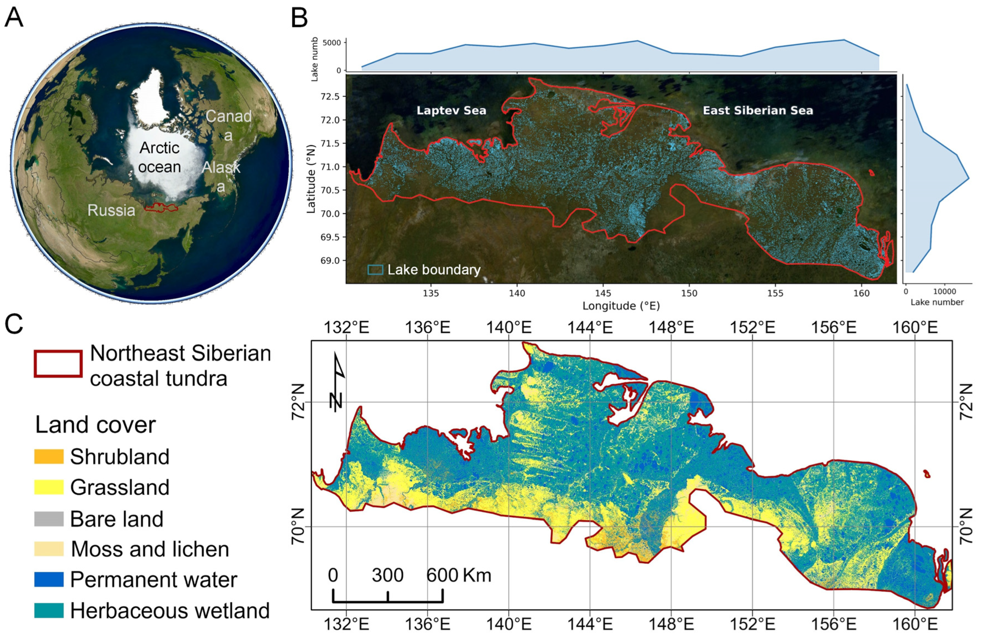
The study area is located in Northeast Siberia, within a lake-rich Arctic coastal tundra landscape extending along the Laptev Sea and East Siberian Sea (Figure 1) [30]. It covers Arctic lowland permafrost terrain between approximately 68.6–72.7°N and 130.7–161.7°E. The region is characterized by extensive ice-rich permafrost, low-relief topography, poor surface drainage, and a high density of thermokarst lakes [31,32]. These lakes are sensitive to thaw-related ground subsidence, shoreline erosion, snowmelt runoff, seasonal water-balance variation, and the development of drainage pathways [32]. As a result, lake expansion, contraction, partial drainage, and post-disturbance vegetation succession can occur within the same broad permafrost landscape [33,34]. The study area lies within the “very high” thermokarst-landscape class (60–100% fractional thermokarst coverage) in the circumpolar classification of Olefeldt et al. [31], which supports the use of thermokarst lakes as the target lake population in this region.

The region is suitable for examining the relationship between lake water-area dynamics and aquatic vegetation change for three reasons. First, the abundance of small and medium-sized lakes allows trajectories of individual lakes to be analyzed beyond regional water-area totals. Second, many lakes are shallow and have broad littoral or nearshore zones, providing potential habitat for emergent, floating, and submerged aquatic vegetation [10,28]. Third, the strong seasonality of temperature, snow cover, thawing, and surface-water availability provides a useful setting for assessing climatic controls on aquatic vegetation dynamics [29].

2.2. Data

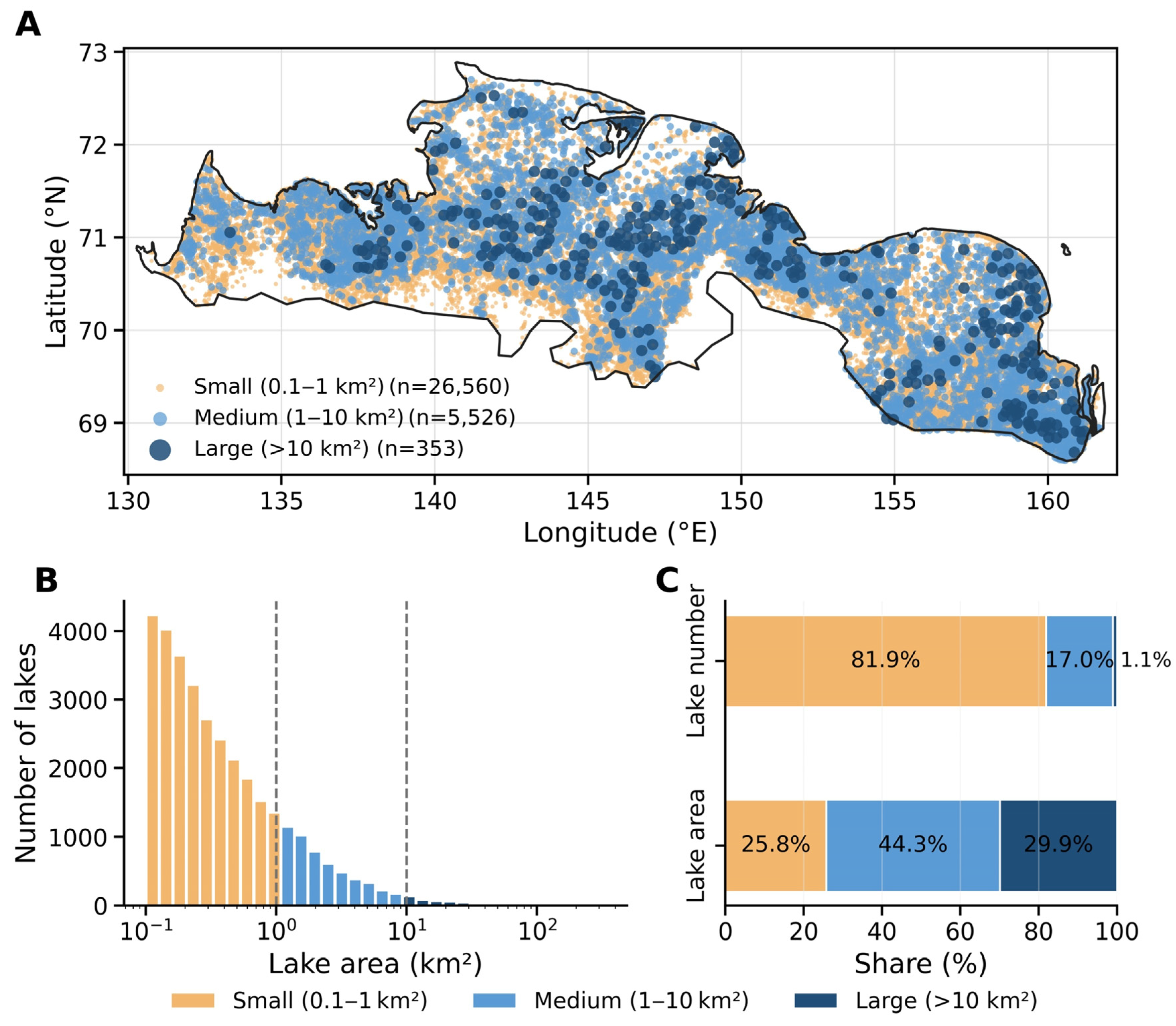
Lake objects and static lake attributes were obtained primarily from the GLAKES inventory, with HydroLAKES used as an auxiliary inventory [35,36]. GLAKES represents a long-term maximum lake extent, whereas HydroLAKES polygons originate from heterogeneous source dates; exact boundary agreement between the two datasets was therefore not expected. The GLAKES lake object was retained as the fixed analysis envelope, and HydroLAKES records were used for cross-checking rather than appended as additional lake objects, preventing duplicate counting of overlapping records. We retained lake objects with boundary area ≥ 10 ha (0.1 km²). This threshold matches the minimum HydroLAKES lake size and corresponds to approximately 111 Landsat 30 m pixels, reducing sensitivity to isolated pixels, mixed shorelines, and unstable delineation in very small ponds. The resulting inventory contained 32,439 lakes: 26,560 small lakes (0.1–1 km²), 5526 medium lakes (1–10 km²), and 353 large lakes (>10 km²).

Annual lake water-area dynamics were characterized using the global surface water dynamics product published by the Global Land Analysis and Discovery (GLAD) team. The GLAD product is based on long-term Landsat observations and provides annual information on surface water-occurrence probability at 30 m spatial resolution [37,38]. This probability-based representation is suitable for Arctic lake analysis because many lake margins contain mixed pixels, shallow water, aquatic vegetation, and seasonal water fluctuations [13,14,15,28]. The GLAD annual product was used to derive a continuous lake water area record from 1999 to 2025. During quality control, 1999 was excluded from the main analysis because regional water area was anomalously low and aquatic vegetation records for 1999 contained substantially more missing and zero values than those for subsequent years. The main analysis period was therefore defined as 2000 to 2025.

Landsat surface reflectance imagery [39,40] was used to derive annual aquatic vegetation metrics. We used Landsat-5 TM, Landsat-7 ETM+, Landsat-8 OLI, and Landsat-9 OLI-2 Collection 2 Level-2 images available in Google Earth Engine [41]. The Landsat analysis window was 1 June–31 August, matching the open-water and main vegetation growing season used in this study. Mission-specific Collection 2 scale factors and quality masks were applied, and corresponding visible, near-infrared, and shortwave-infrared bands were mapped to a common band scheme before classification. Following the aquatic vegetation workflow of Liu et al. [28], no additional empirical linear transformation among Landsat sensors was applied; the same CIE-based classification criteria were used for all missions. Cloud, cloud shadow, snow, radiometrically saturated, and other poor-quality pixels were removed using the quality assessment bands [39,40,41,42]. Because the study region spans several Landsat paths, observation availability varies among lake-years and is treated as a data-quality consideration rather than represented by a single regional scene count.

Climate variables were derived from the ERA5-Land reanalysis dataset [43,44]. ERA5-Land provides spatially continuous land-surface climate variables at high temporal resolution and is suitable for extracting climate indicators over data-sparse Arctic regions [43]. We selected six variables relevant to aquatic vegetation growth. Thermal conditions were represented by growing-season mean 2 m air temperature and surface-soil temperature; moisture conditions by growing-season precipitation, precipitation minus evapotranspiration (P−ET), and surface-soil moisture; and May–July cumulative snowmelt. Growing-season variables were calculated for June–August, while snowmelt was accumulated from May to July. Air and soil temperatures were expressed in degrees Celsius. Precipitation, P−ET, and snowmelt were expressed in millimeters, and soil moisture as volumetric water content. Because the ERA5-Land grid was substantially coarser than most individual lakes, climate variables were sampled at lake centroids. Annual values and their anomalies relative to the local 2000–2025 means were retained for subsequent analysis.

2.3. Methods

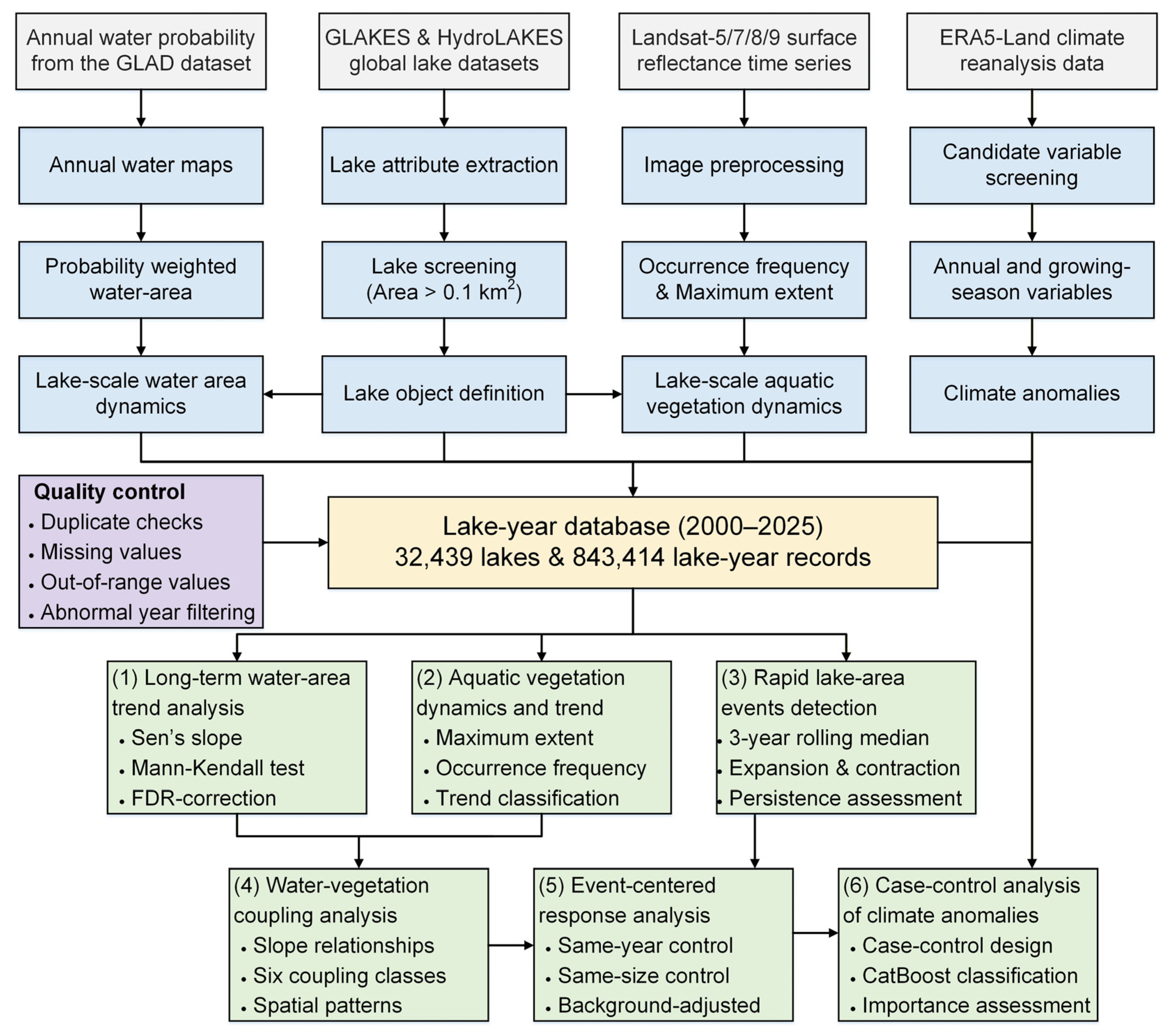
Figure 2 summarizes the overall workflow of this study. We integrated lake boundary datasets, GLAD annual surface-water probability products, Landsat surface-reflectance imagery, and ERA5-Land climate variables to construct a lake-year database for 2000–2025. Annual lake water area was estimated using a probability-weighted approach, while aquatic vegetation occurrence frequency and maximum extent were derived from Landsat-based aquatic vegetation mapping. Following quality control, the database was used for six complementary analyses: (1) long-term water-area trend analysis; (2) aquatic vegetation dynamics and trend classification; (3) detection of rapid lake-area expansion and contraction events; (4) long-term water–vegetation coupling analysis; (5) event-centered analysis of water-area and vegetation responses; and (6) case–control analysis of climate anomalies associated with rapid aquatic vegetation increase events.

2.3.1. Extraction of Lake Water Area and Aquatic Vegetation Metrics

Annual lake water area was calculated for each lake-object using the GLAD annual surface water probability product. Instead of using a binary water mask, we applied a probability-weighted area calculation to reduce the influence of mixed shoreline pixels and year-to-year classification uncertainty [37,38]. For each lake i and year t, all GLAD pixels located within the lake boundary were identified. The contribution of each pixel was weighted by its annual water probability:

$$A_{i,t}={\sum }_{p\in i}{a}_p\times {\displaystyle \frac{P_{p,t}}{100}}$$

(1)

where $A_{i,t}$ is the annual water area of lake i in year t, $a_p$ is the area of pixel p, and $P_{p,t}$ is the GLAD annual water probability of pixel p in year t. This calculation produced a continuous annual water-area estimate rather than a binary water/non-water area. Annual water area was converted to square kilometers for subsequent analysis. Here, “mapped lake water area” denotes the GLAD probability-weighted water signal within the fixed lake envelope; it should not be interpreted as complete hydrologic inundation beneath dense aquatic vegetation, which can reduce water-like spectral reflectance.

Aquatic vegetation was extracted from Landsat observations using the automatic detection approach of Liu et al. [28]. Red, green, and blue surface reflectance was transformed to CIE x–y chromaticity coordinates, and initial vegetation candidates were selected using the lower boundary y > 11.102568x² − 6.495907x + 1.309264. Following the East Siberian implementation in Liu et al. [28], a 97% long-term water-occurrence threshold was used to constrain the potential aquatic vegetation zone within each lake object.

Candidate pixels were further screened using the criteria of Liu et al. [28]. Pixels with red-minus-SWIR reflectance greater than zero were removed to reduce algal-bloom contamination; the outermost pixel of the potential aquatic habitat was excluded to reduce confusion with adjacent terrestrial and wetland vegetation; pixels with an RGB spectral angle of 172.6° or less were removed to reduce mudflat-vegetation contamination; and pixels satisfying NDVI < 0.47 and NDWI > −0.24 were excluded as spectrally abnormal water pixels. These spatial and spectral constraints reduce the chance that dry terrestrial revegetation on exposed margins is counted as aquatic vegetation, although mixed transitional wetland pixels remain a source of uncertainty. The resulting maps mainly represent emergent and floating aquatic vegetation. Submerged vegetation is likely underestimated because of water-column attenuation and the limited sensitivity of 30 m Landsat imagery [13,15,28].

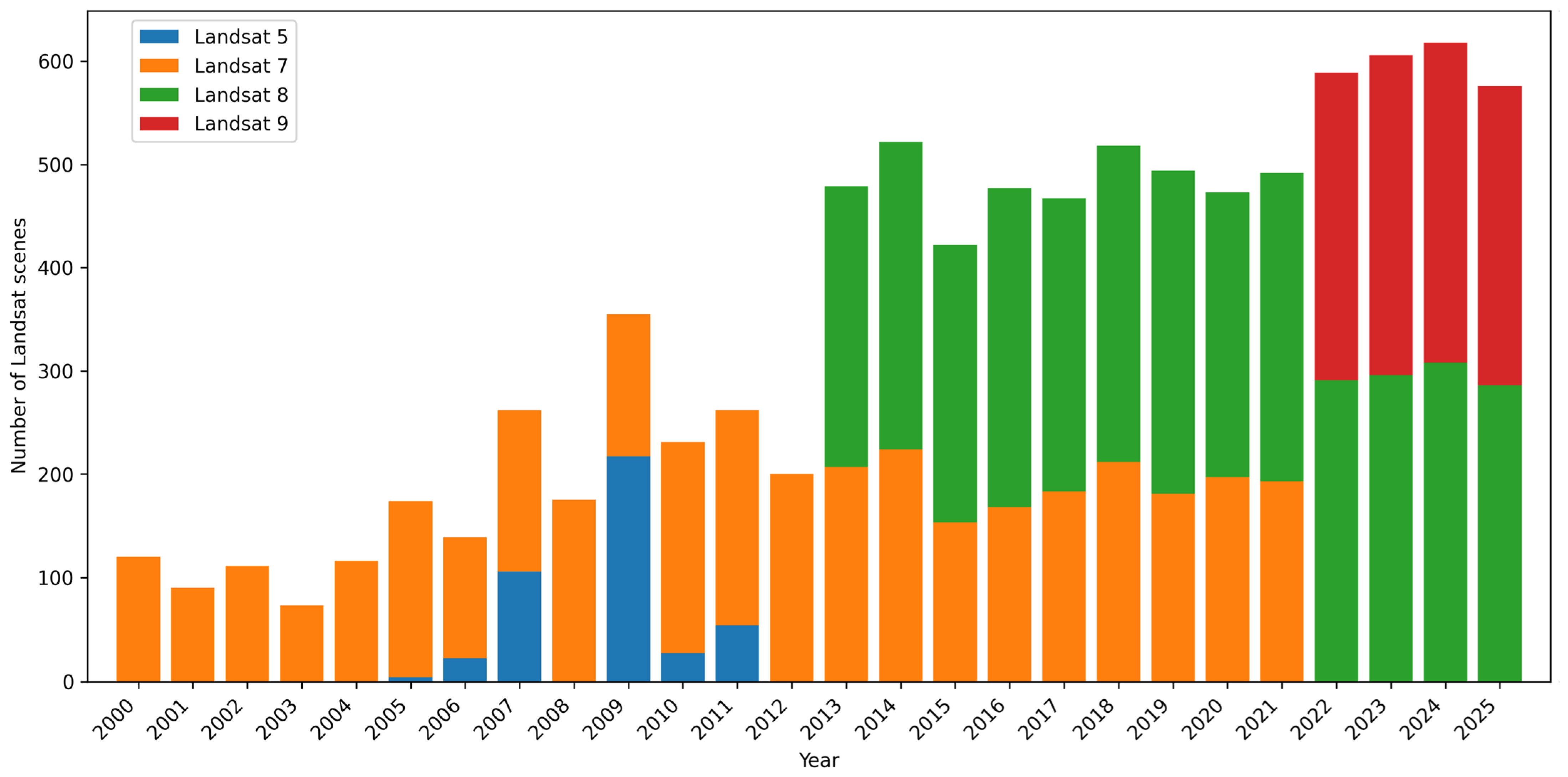
Two annual aquatic vegetation metrics were calculated for each lake. Occurrence frequency was calculated by pooling all valid pixel observations within a lake-year: the numerator was the number of valid pixel observations classified as aquatic vegetation, and the denominator was the total number of valid cloud-free pixel observations. It was not calculated by first estimating a frequency for each pixel and then averaging pixel-level frequencies. Maximum extent was calculated separately as the largest aquatic vegetation area mapped in any valid observation during that year. The regional annual maximum extent reported below is the sum of lake-level maxima and therefore does not represent a simultaneous regional vegetation map. Both aquatic vegetation metrics may be influenced by observation availability, and annual maximum extent has a greater chance of capturing the seasonal peak when scene availability is higher. We therefore interpret isolated annual extremes cautiously and rely primarily on multi-year contrasts and lake-level trends for the long-term conclusions. To assess the potential influence of observation availability, we summarized the annual number of Landsat 5, 7, 8, and 9 scenes intersecting the study area during the June–August analysis period (Figure A1).

2.3.2. Lake-Year Database and Long-Term Trend Analysis

All annual water area, aquatic vegetation occurrence frequency, aquatic vegetation maximum extent, lake inventory attributes, and climate variables were harmonized by lake ID and year to construct a lake-year database for 2000 to 2025. Water area and aquatic vegetation maximum extent were stored in square kilometers, while aquatic vegetation occurrence frequency was retained as a percentage. The final table included annual water area, aquatic vegetation occurrence frequency, aquatic vegetation maximum extent, boundary area, size class, longitude, latitude, perimeter, shoreline complexity, climate variables, and quality control flags.

The final analysis database contained 843,414 lake-year observations, representing 32,439 lakes over 26 years. Before analysis, we screened for duplicate lake-year records; missing observations; negative, out-of-range, or abnormal zero values; inconsistencies between boundary and annual water area; and regionally anomalous vegetation behavior. Years 2003, 2004, 2006, 2007, and 2009 were flagged as vegetation caution years because of elevated missingness or abrupt regional behavior. These years were retained in the primary time series but were not interpreted individually as evidence of abrupt ecological transitions. Quality control flags were retained in the lake-year database.

Long-term trends were calculated separately for annual water area, aquatic vegetation occurrence frequency, and maximum extent. For each lake, the Mann–Kendall test [45] evaluated monotonic trends, and Sen’s slope [46] estimated their direction and rate. Because tests were repeated across many lakes, p-values were adjusted using the false discovery rate [47].

Trend classification combined statistical significance with a practical change magnitude. For lake water area, the full-period cumulative change was derived from Sen’s slope and expressed relative to the lake’s median water area. Lakes were classified as expanding or contracting when the false discovery rate (FDR) adjusted q-value was ≤0.05 and the cumulative Sen’s-slope change was ≥10% or ≤−10% of median water area, respectively. The 10% magnitude criterion was used together with statistical significance to avoid classifying very small but statistically detectable changes over a 26-year series. Lakes not meeting both criteria were classified as stable or weakly changing. For maximum vegetation extent, the main classification required an absolute cumulative change of at least 1 ha in addition to the relative criterion; the earlier 0.1 ha rule was retained as a sensitivity check because 0.1 ha is close to a single Landsat-scale pixel. A similar classification logic was applied to occurrence frequency. Trend results were summarized at regional and lake-object scales and by lake size class.

2.3.3. Detection of Abrupt Lake Expansion and Contraction Events

Abrupt lake expansion and contraction events were identified separately from long-term trends [33]. Sen’s slope describes the overall direction and rate of monotonic change but does not locate abrupt annual shifts [34]. Previous studies have successfully applied temporal-segmentation methods such as LandTrendr to identify lake drainage events [21,48,49]. However, LandTrendr is primarily suited to detecting abrupt directional changes such as rapid lake contraction and is less effective for identifying lake expansion [34]. Here we used a simpler rule-based detector applied to the object-level annual lake-area series, allowing both abrupt lake expansion and contraction events to be identified consistently.

To reduce isolated single-year noise, each annual water-area series was smoothed using a centered three-year rolling median, and change was calculated relative to the preceding smoothed year. Because a centered three-year filter uses information from adjacent years, the assigned event year should be interpreted at annual resolution with approximately ±1-year timing uncertainty. Candidate events were classified as rapid expansions or contractions when the absolute relative change exceeded 20%, or the absolute area change exceeded 10 ha. The relative threshold captures substantial changes in small lakes, while the 10 ha threshold (about 111 Landsat 30 m pixels) captures large absolute changes in larger lakes and reduces sensitivity to isolated pixel-scale errors. These are conservative operational thresholds for regional screening and are not interpreted as a formal product-error bound.

Candidate changes in the same type occurring no more than two years apart within a lake were treated as one event episode, and the strongest candidate in each episode was retained. When a lake contained multiple retained episodes, the strongest episode was used as the main event for the aligned trajectory analysis. For each event, we recorded lake ID, event year, event type, pre-event and post-event area, absolute and relative change, and lake size class. Persistence was evaluated using the mean water area during t = +1 to +3 relative to the pre-event baseline at t = −3 to −1 and normalized by the event-year change. Events retaining at least 50% of the detected change were labeled persistent; the remainder were treated as short-term pulses or reversals. The 50% rule is an operational distinction between changes that retained most of their magnitude and those that substantially reversed.

2.3.4. Event-Centered Responses and Long-Term Water–Vegetation Coupling

Rapid aquatic vegetation increase events were identified from annual maximum vegetation extent using the same three-year centered rolling median. An increase was considered an event when it was at least 1 ha and either exceeded 20% of the preceding smoothed extent or was greater than 10 ha. The 1 ha minimum corresponds to approximately 11 Landsat 30 m pixels and avoids treating one-pixel changes as regional-scale events. To avoid unrealistically large proportional changes when vegetation first appeared, the denominator for relative change was constrained to at least 1 ha. Candidate events no more than two years apart were treated as one episode and the strongest candidate was retained; the strongest retained episode per lake was used as the main event. Threshold sensitivity was additionally evaluated across minimum changes of 1–5 ha and relative changes of 15–30% as a robustness check on event counts.

We conducted two complementary event-centered analyses, one centered on rapid lake-area expansion and contraction and the other on rapid aquatic vegetation increase. For each main event, the event year was t = 0, and annual water area, maximum vegetation extent, and occurrence frequency were aligned from t = −5 to t = +5. The five-year window was selected to capture both immediate and multi-year post-event trajectories while retaining a large event sample. The mean from t = −3 to t = −1 was used as the pre-event baseline. Requiring a complete ±5-year window restricts the primary event-centered sample to event years 2005–2020; the 2000–2025 period refers to the full long-term time series.

Background controls were constructed separately for water area and vegetation-centered analyses. For each event year and lake size class, the control pool included all lakes in the same size class that had no corresponding event within three years before or after the focal year. Events occurring in the same year and size class therefore shared the same control pool, while the eligible controls could vary among event years. We employed a difference in differences approach for background correction by comparing changes in event lakes with concurrent changes in control lakes [50,51]. For each relative year, changes in control lakes were calculated relative to their own pre-event baseline (t = −3 to −1), and the median control change was calculated separately for each event year, size class, relative year, and response metric. This median was then subtracted from the corresponding event trajectory. Years with unusually many synchronous events, defined as annual counts above the median plus three scaled median absolute deviations, were excluded from the primary trajectories.

Long-term water–vegetation coupling was evaluated separately from the event-centered analysis. For the full lake population and each size class, we calculated Pearson and Spearman correlations between water-area Sen’s slopes and the corresponding slopes of occurrence frequency and maximum vegetation extent. Pearson correlation was used to quantify linear association, whereas Spearman correlation was used to evaluate whether the two trends showed a consistent monotonic relationship.

Lakes were then assigned to six mutually exclusive coupling classes by combining three water-area states with two vegetation states. Water area was classified as expansion, stable or weak change, or contraction using the Mann–Kendall FDR-adjusted significance, Sen’s slope direction, and a cumulative-change threshold of 10% of median water area. For maximum vegetation extent, vegetation increase required an FDR-adjusted q-value ≤ 0.05, a positive Sen’s slope, and a cumulative increase of at least the larger of 1 ha or 10% of median vegetation extent. For occurrence frequency, vegetation increase required an FDR-adjusted q-value ≤ 0.05, a positive Sen’s slope, and a cumulative increase of at least the larger of 1 percentage point or 10% of the median occurrence frequency. All remaining lakes were retained in the operational stable (or weakly changing) vegetation group. This is effectively a non-increasing group and includes the 28 lakes (0.09%) with decreasing maximum extent.

The resulting classes were: water expansion with vegetation increase, water expansion with stable vegetation, stable or weakly changing water area with vegetation increase, stable or weakly changing water area with stable vegetation, water contraction with vegetation increase, and water contraction with stable vegetation. Coupling was classified separately for maximum vegetation extent and occurrence frequency. Class proportions were summarized for the complete lake population and each lake-size class, and their spatial distributions were mapped.

2.3.5. Case–Control Analysis of Climate Anomalies Affecting Aquatic Vegetation Events

We used a same-lake case–control classification design to examine climatic conditions associated with rapid aquatic vegetation increase events. Positive observations were main vegetation increase events with complete five-year windows before and after the event, so eligible event years were 2005–2020. Regionally synchronous anomalous years were excluded. Control observations were non-event years from the same lakes and were restricted to the same 2005–2020 period. Years located within two years before or after any detected vegetation increase event in the same lake were excluded from the control pool. The ±2-year exclusion window was used to remove years immediately surrounding an event, which may share short-term climatic or ecological conditions associated with the detected vegetation increase, while retaining sufficient non-event years for within-lake control selection. Two controls were retained per event lake, preferentially one before and one after the event; if no eligible year was available on one side, an additional eligible year from the remaining side was used. No fixed temporal distance was imposed beyond these restrictions. The final matched dataset contained 10,409 lakes and 31,227 lake-year observations, with one event year and two controls per lake.

The six climate variables described in Section 2.2 were used as model predictors [43,44]. For each lake and year, climate anomalies were calculated by subtracting the local 2000–2025 mean from the annual value. These anomalies indicate whether an event year was warmer or wetter than usual at that lake, and whether it had more or less snowmelt. Because event and control observations were drawn from the same lake, time-invariant lake attributes and geographic location were implicitly controlled by the matched design.

A CatBoost gradient-boosted decision-tree classifier was used to distinguish vegetation increase event years from matched non-event years [52]. CatBoost was selected because it can represent nonlinear relationships and predictor interactions. Similar models have been used to estimate thermokarst-lake drainage probability and examine environmental controls on drainage in Northeast Siberia and St. Lawrence Island [23,30]. The model consisted of 250 trees with a maximum depth of 5 and a learning rate of 0.07. Class weights of 1 and 2 were assigned to the control and event classes, respectively.

Model performance was assessed using five-fold stratified cross-validation grouped by lake ID, ensuring that observations from the same lake did not occur in both training and validation data within a fold. Out-of-fold predictions were evaluated using the area under the receiver operating characteristic curve (ROC–AUC), average precision, balanced accuracy, sensitivity, specificity, precision, F1 score, and Brier score. Confidence intervals for ROC–AUC and average precision were obtained by nonparametric bootstrap resampling of the pooled out-of-fold predictions. A model based on the original climate values was fitted as a sensitivity analysis. An additional validation grouped observations sharing identical ERA5-Land climate values in the same year to prevent exact duplicate climate records from being split across folds; this check does not remove all spatial or year-level dependence. Leave-one-calendar-year-out validation was therefore used as the stricter test of temporal transferability.

Predictor importance was evaluated using SHapley Additive exPlanations (SHAP) values and permutation importance [53,54]. Mean absolute SHAP values from out-of-fold predictions summarized how strongly each predictor contributed within the fitted model, and SHAP dependence plots described the direction and nonlinearity of model responses [54]. Permutation importance measured the decrease in validation ROC–AUC after a predictor was permuted. Because both measures explain the same fitted CatBoost model, agreement between them was treated as within-model consistency rather than independent validation. Correlated predictors can share or redistribute importance; percentages are therefore interpreted as relative model importance and not as the percentage contribution of a climate variable to the underlying ecological process.

3. Results

3.1. Spatiotemporal Patterns of Water-Area Dynamics

A total of 32,439 lakes larger than 0.1 km² were selected for analysis within the Northeast Siberian coastal tundra, with a combined lake boundary area of approximately 31,898 km² (Figure 3). Spatially, lakes were distributed across the entire study area, but their density was not uniform. High lake densities were especially evident in the central and eastern lowland sectors, whereas the western margin contained comparatively fewer lakes. Small lakes dominated the landscape numerically and occurred almost continuously throughout the region, while medium and large lakes were less numerous but were also widely distributed (Figure 3A). The lake-size distribution was strongly right-skewed (Figure 3B). Small lakes (0.1–1 km²) accounted for 81.9% of lake objects but only 25.8% of total boundary area, whereas medium and large lakes together represented 18.1% of lake number and 74.2% of lake area (Figure 3C). This contrast motivated the size-stratified analyses used throughout the study.

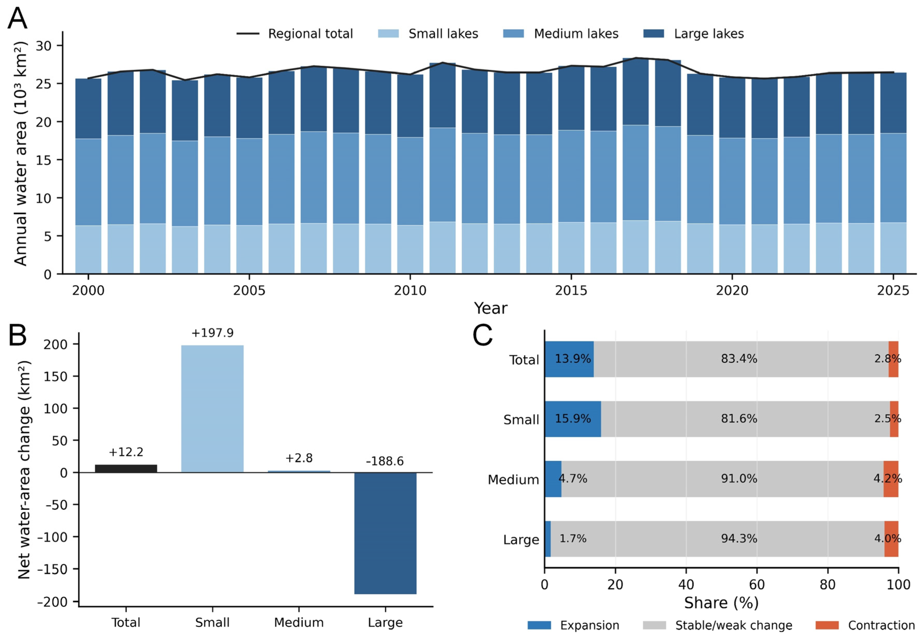
At the regional scale, total lake water area remained remarkably stable during 2000–2025 (Figure 4A). Mean regional water area was 26,141.4 km² during 2000–2004 and 26,153.5 km² during 2021–2025, corresponding to a net increase of only 12.2 km², or about 0.05% (Figure 4B). Interannual fluctuations were evident, but these were modest relative to the total regional water area. This apparent regional stability masked contrasting size-dependent changes. Small lakes showed a net gain of 197.9 km² between the early and late periods, and medium lakes increased slightly by 2.8 km², whereas large lakes showed a net loss of 188.6 km² (Figure 4B). As a result, gains in numerous smaller lakes were almost entirely offset by losses in a much smaller number of large lakes, producing little net regional change.

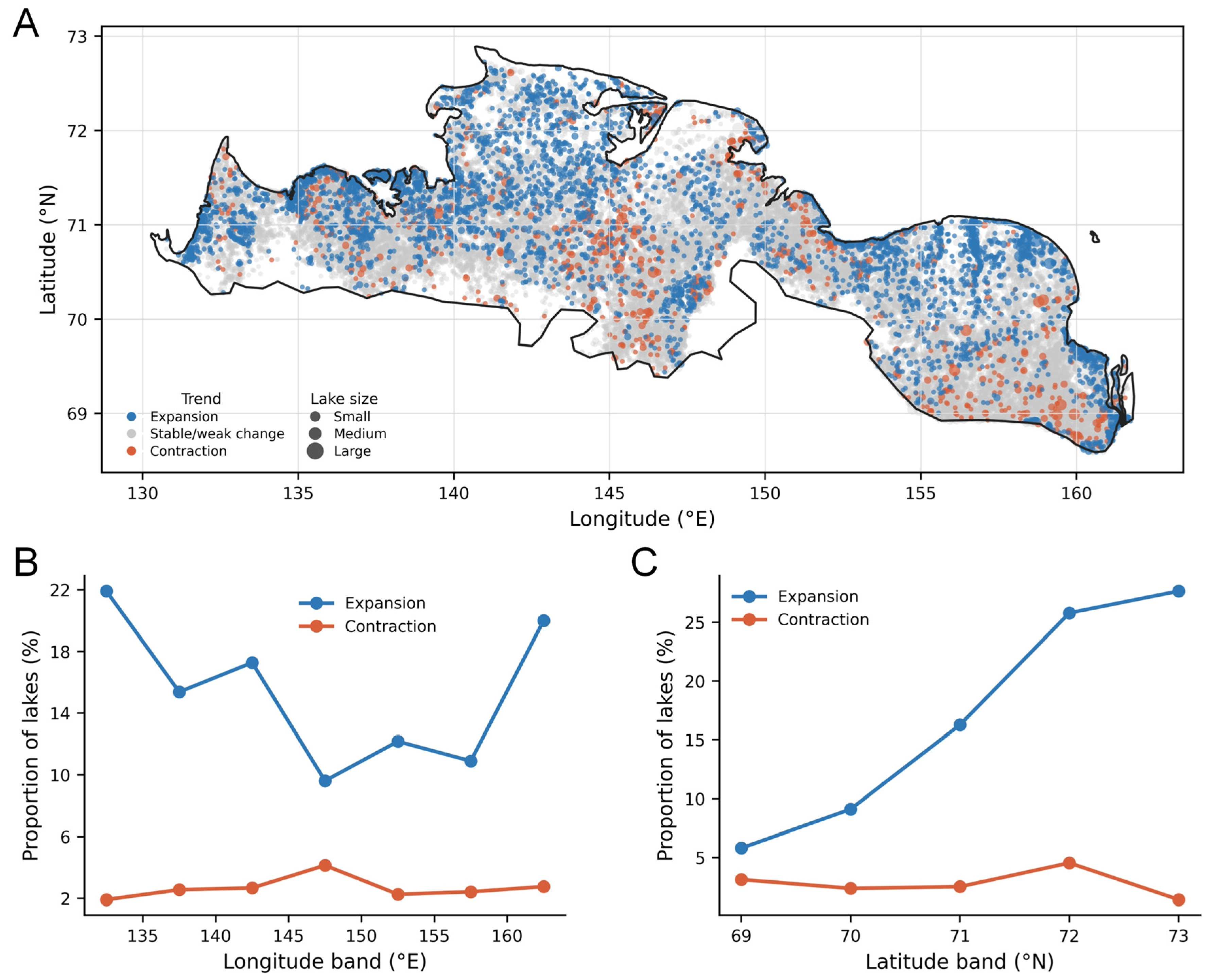
Trend classification further showed that most lakes were stable or only weakly changing under the conservative threshold definition, but expanding lakes clearly outnumbered contracting lakes (Figure 4C). Across all lakes, 13.9% were classified as expanding, 2.8% as contracting, and 83.4% as stable or weakly changing. Expansion was most common in the small-lake class, where 15.9% of lakes expanded and only 2.5% contracted. In contrast, medium and large lakes showed much lower expansion proportions (4.7% and 1.7%, respectively), while contraction remained relatively more important in these larger size classes (4.2% and 4.0%, respectively). These results indicate that the long-term water-area record was characterized by near-balance at the regional scale, but with a clear tendency toward more frequent expansion among small lakes and more limited but important area losses among large lakes.

The spatial distribution of trend classes revealed that stable or weakly changing lakes dominated across the study region, but expanding and contracting lakes were widely distributed rather than confined to a single subregion (Figure 5A). Expanding lakes were more numerous than contracting lakes throughout most of the study area, although both classes occurred in all major lake clusters. Contracting lakes were comparatively sparse and appeared as scattered hotspots embedded within broader zones dominated by stable or expanding lakes.

The longitudinal analysis showed a distinctly uneven east–west pattern in the proportion of expanding lakes (Figure 5B). Expansion exceeded 20% in the westernmost band (130–135°E) and again in the far eastern sector (160–165°E), while the central part of the study area generally showed lower values, especially around 145–150°E, where the expansion proportion declined to about 9.6%. Contraction remained much lower across all longitude bands, mostly around 2–3%, but reached a local maximum of about 4.1% in the 145–150°E band. This pattern suggests that the strongest long-term increases in lake water area were concentrated in the western and eastern margins of the study region, whereas the central sector was comparatively less dynamic in terms of expansion.

A clearer gradient emerged along latitude (Figure 5C). The proportion of expanding lakes increased northward, from 5.8% in the southernmost band (68.5–69.5°N) to 25.8% in 71.5–72.5°N, and further to 27.7% in the northernmost band. By contrast, contraction remained consistently low across latitude bands, generally between about 2.4% and 4.6%, without a similarly strong monotonic trend. Taken together, these results indicate that long-term lake expansion became progressively more common toward higher latitudes, whereas lake contraction remained a secondary process with a weaker geographic structure. Since the study area extends along the Arctic coast, higher latitudes are also generally closer to the coastline. Because latitude and distance to the coast covary within the study area, their respective contributions cannot be separated from the present analysis.

3.2. Temporal Changes in Aquatic Vegetation Extent and Occurrence Frequency

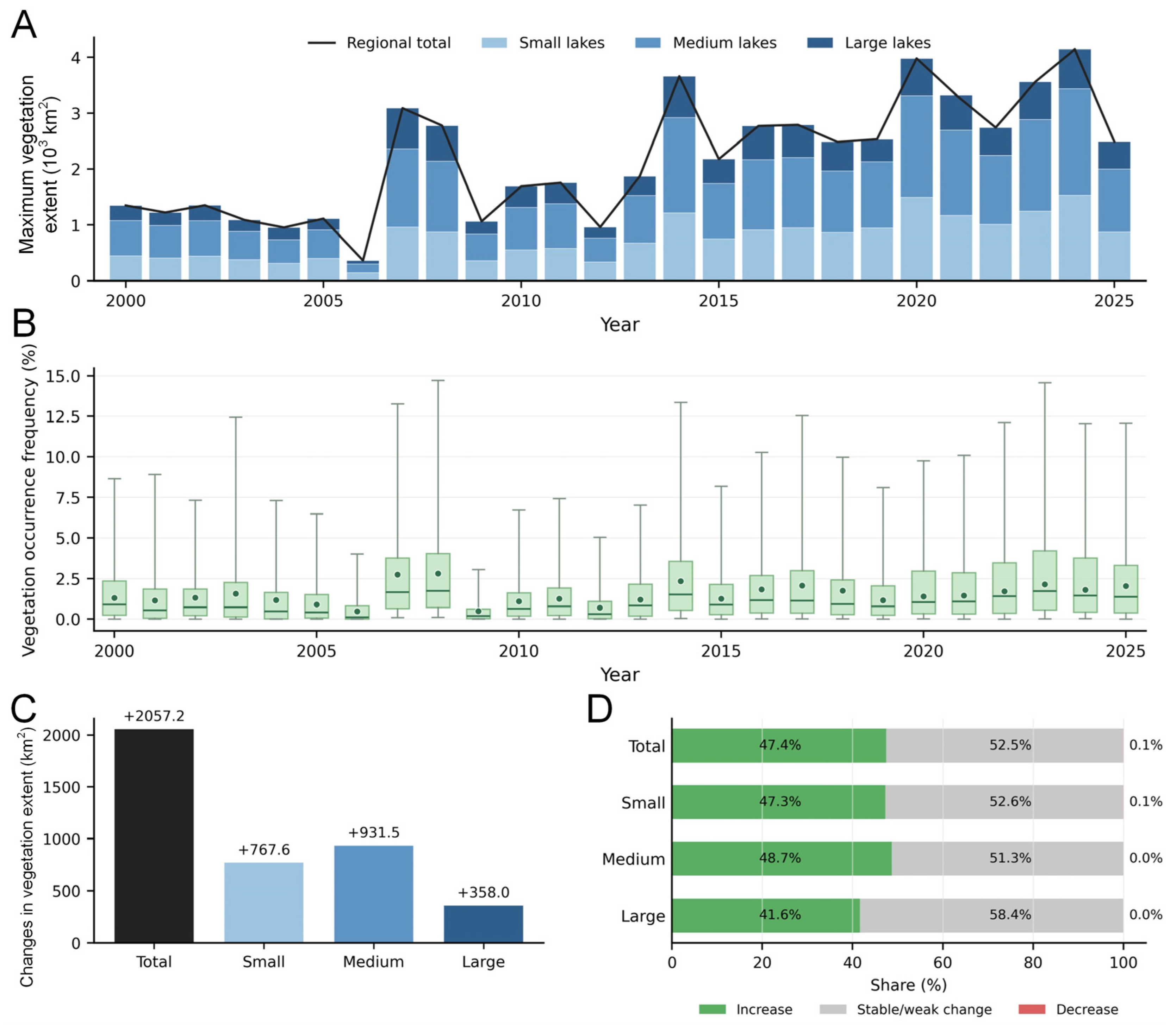
Aquatic vegetation showed a pronounced increase in annual maximum mapped extent during 2000–2025, with substantial interannual variability (Figure 6A). Mean regional maximum extent increased from 1192.8 km² during 2000–2004 to 3250.0 km² during 2021–2025, a gain of 2057.2 km² (172.5%; Figure 6C). The regional value is the sum of the annual maximum extent of individual lakes, and those lake-level maxima may occur on different dates. It therefore represents an annual regional index of maximum mapped extent, not a simultaneous vegetation area on one date. Over the same two periods, the ratio of this index to regional lake water area increased from 4.56% to 12.42%.

The maximum-extent time series contained pronounced annual fluctuations. Regional maximum extent reached its lowest value in 2006 (363.0 km²) and exceeded 3000 km² in 2007. Other high values occurred in 2014, 2020, 2023, and 2024, with a maximum of 4141.0 km² in 2024. Because 2006 and 2007 fall within the vegetation caution years identified during quality screening, this sharp year-to-year contrast is not interpreted as a single ecological step change. The long-term conclusion is based on multi-year means and lake-level trends rather than on these two annual values.

Landsat scene availability varied substantially over the study period (Figure A1). The total number of scenes intersecting the study area averaged 177.5 per year during 2000–2012, increased to 482.7 during 2013–2021, and further increased to 597.3 during 2022–2025. Scene availability increased from 139 in 2006 to 262 in 2007, which may have contributed to the pronounced vegetation contrast between these two years. However, the low vegetation extent in 2006 cannot be attributed to observation availability alone. The 139 scenes available in 2006 were comparable to, or more numerous than, those available in most years during 2000–2005 (73–174 scenes), when similarly low vegetation extent was not consistently observed. Moreover, scene availability remained relatively high after 2013, while substantial interannual variation in vegetation extent persisted. Differences in observation availability may therefore contribute to individual annual fluctuations, including the 2006–2007 contrast, but do not provide a sufficient explanation for either the exceptionally low value in 2006 or the long-term increase in aquatic vegetation.

Aquatic vegetation occurrence frequency also increased, but less strongly than maximum extent (Figure 6B). The water-area-weighted mean occurrence frequency increased from 1.30% during 2000–2004 to 1.83% during 2021–2025, corresponding to an increase of 0.53 percentage points, or 40.6%. The mean of the annual lake-scale medians increased from 0.67% to 1.40%, while the mean annual 75th percentile increased from 1.99% to 3.52%. The weighted occurrence frequency was lowest in 2006, at 0.48%, and highest in 2008, at 2.81%. The different peak years are consistent with the two metrics capturing different dimensions of aquatic vegetation dynamics.

All three lake-size classes contributed to the increase in maximum vegetation extent, although their absolute and relative contributions differed (Figure 6C). Medium lakes showed the largest absolute increase, from 554.9 to 1486.5 km², yielding a gain of 931.6 km² and accounting for 45.3% of the regional increase. Small lakes increased by 767.6 km² and contributed 37.3% of the total gain, while large lakes increased by 358.0 km² and contributed the remaining 17.4%. In relative terms, the increase was strongest in small lakes (+193.3%), followed by medium (+167.9%) and large lakes (+148.7%). A similar size dependence was evident in occurrence frequency: the water-area-weighted mean increased by 0.91 percentage points in small lakes, compared with 0.48 percentage points in medium lakes and 0.27 percentage points in large lakes.

Long-term trend classification confirmed that increases in maximum mapped extent were widespread among individual lakes (Figure 6D). Under the combined criteria, 15,392 lakes (47.4%) were classified as increasing, 17,019 lakes (52.5%) were stable or weakly changing, and only 28 lakes (0.09%) were classified as decreasing. The proportion of increasing lakes was highest among medium lakes (48.7%), closely followed by small lakes (47.3%), and was somewhat lower among large lakes (41.6%). Decreases were rare in every size class, accounting for 0.10% of small lakes, 0.04% of medium lakes, and none of the large lakes. Taken together, the two metrics indicate that aquatic greening was expressed primarily through expansion of the annual maximum mapped footprint.

3.3. Long-Term Coupling Between Lake Water-Area and Aquatic Vegetation Dynamics

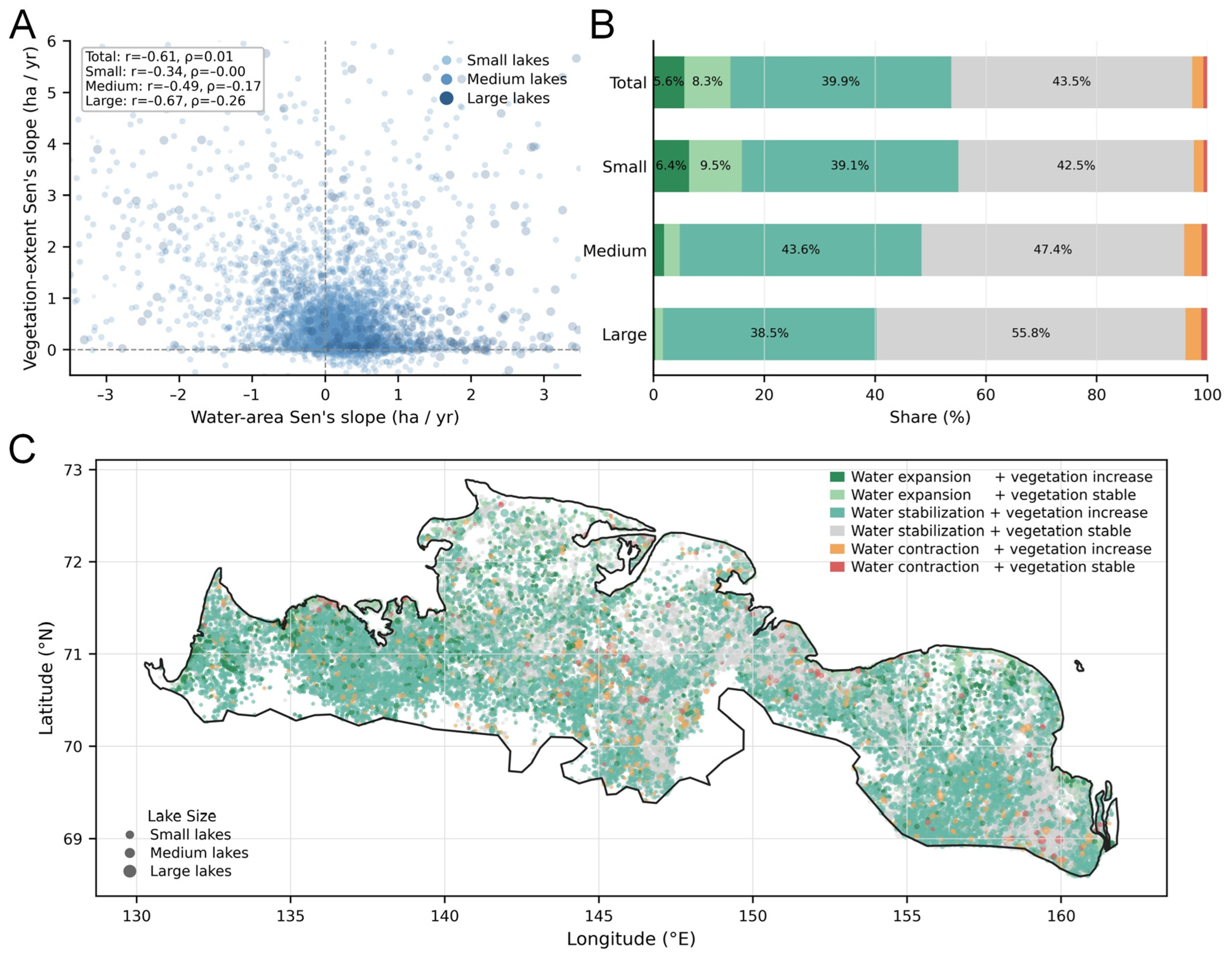
The lake-scale slope relationships differed substantially between the two aquatic vegetation metrics (Figure 7 and Figure 8). For maximum mapped vegetation extent (Figure 7), the Pearson correlation between water-area and vegetation slopes was moderately negative for the complete lake population (r = −0.61). Negative Pearson correlations were also obtained for small (r = −0.34), medium (r = −0.49), and large lakes (r = −0.67). However, the corresponding Spearman correlations were close to zero for all lakes (ρ = 0.01) and small lakes (ρ ≈ 0), and remained relatively weak for medium (ρ = −0.17) and large lakes (ρ = −0.26). The divergence between Pearson and Spearman coefficients indicates that the linear relationship was sensitive to lakes with large absolute changes and was not a consistent monotonic pattern across the full lake population.

The coupling-class composition provides a clearer description of the dominant long-term trajectories (Figure 7B). Across all lakes, 43.5% were characterized by both stable water area and stable vegetation extent, while a further 39.9% showed increasing maximum vegetation extent despite stable water area. Water expansion accompanied vegetation increase in 5.6% of lakes, whereas 8.3% experienced water expansion without a classified increase in vegetation extent. Water contraction was uncommon: 2.0% of lakes combined contraction with vegetation increase, and only 0.8% combined contraction with stable vegetation.

Coupling patterns also varied with lake size. The combination of water expansion and vegetation increase accounted for 6.4% of small lakes, but only 1.9% of medium lakes and 0.3% of large lakes. Conversely, the proportion showing stability in both water area and vegetation extent increased from 42.5% in small lakes to 47.4% in medium lakes and 55.8% in large lakes. Vegetation increases under stable water conditions remained common in all size classes, accounting for 39.1% of small lakes, 43.7% of medium lakes, and 38.5% of large lakes. Thus, increases in maximum vegetation extent were not confined to expanding lakes and often occurred where total water area remained comparatively stable.

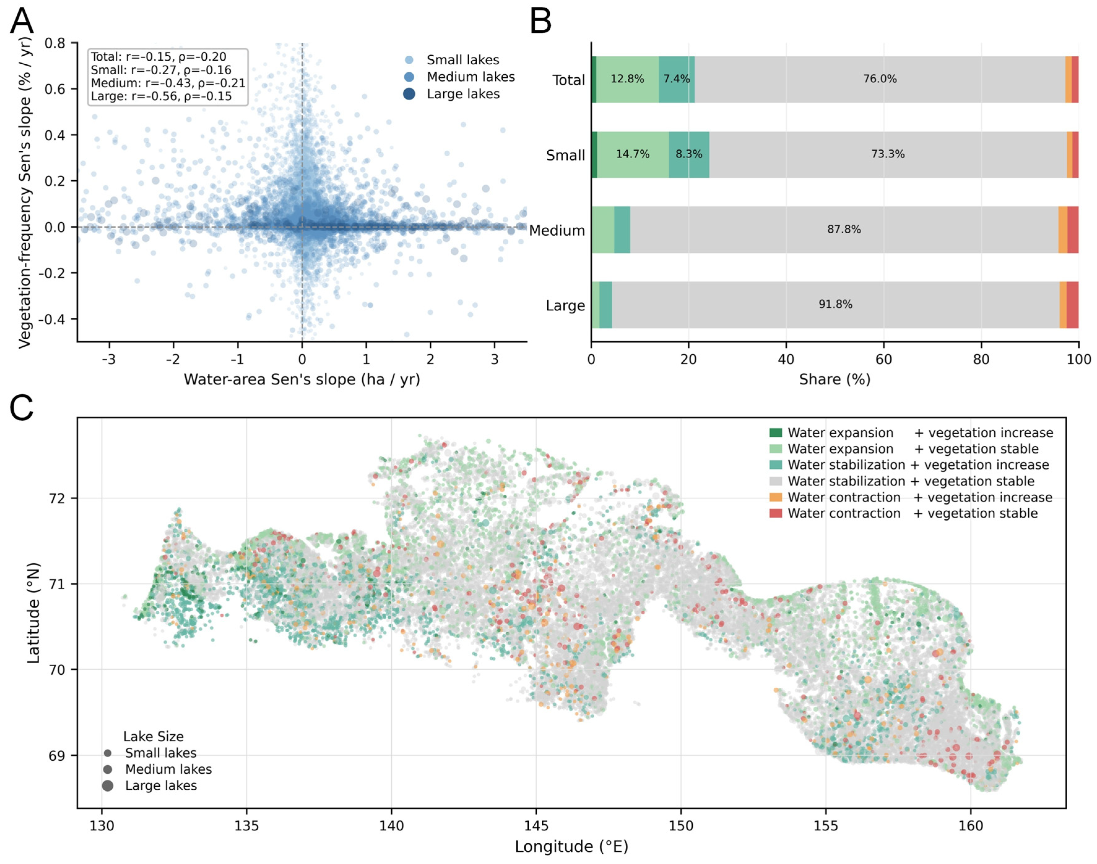
The relationship between water-area changes and vegetation occurrence frequency was weaker than that for maximum extent, but the Pearson and Spearman coefficients were more consistent in sign (Figure 8A). Across all lakes, the correlations were r = −0.15 and ρ = −0.20. Pearson correlations became progressively more negative from small (r = −0.27) to medium (r = −0.43) and large lakes (r = −0.56), although Spearman correlations remained weak, ranging from −0.15 to −0.21. This suggests a weak tendency for vegetation occurrence frequency to increase more rapidly in lakes with declining or slowly changing water area, but the relationship was highly dispersed and did not represent a strong uniform response across individual lakes.

The occurrence-frequency coupling classification was dominated by stability in both variables (Figure 8B). Stable water area combined with stable vegetation frequency accounted for 76.0% of all lakes, while 7.4% showed increasing vegetation frequency under stable water conditions. Water expansion with stable vegetation frequency accounted for 12.8%, whereas simultaneous water expansion and frequency increase occurred in only 1.0% of lakes. The two water-contraction classes together represented 2.8% of the lake population. Thus, unlike maximum vegetation extent, which increased in nearly half of all lakes, statistically classified increases in vegetation occurrence frequency were limited to approximately 9.7% of lakes.

This contrast was especially clear among different lake-size classes. Stable water area and stable vegetation frequency accounted for 73.3% of small lakes, 87.8% of medium lakes, and 91.8% of large lakes. Simultaneous water expansion and vegetation-frequency increase occurred in 1.2% of small lakes, 0.1% of medium lakes, and none of the large lakes. Water expansion without a corresponding increase in vegetation frequency was also concentrated in small lakes, accounting for 14.7%, compared with 4.6% of medium lakes and 1.7% of large lakes. The occurrence-frequency response was therefore more spatially and numerically restricted than the increase in maximum mapped vegetation extent.

Spatially, the dominant stable–stable classes were distributed throughout the study region, particularly across the central and eastern lake-rich lowlands (Figure 7C and Figure 8C). Coupled water expansion and vegetation increase occurred more frequently in the western and northern parts of the study area and were largely associated with small lakes. Increases in vegetation under stable water-area conditions were more widespread for maximum extent than for occurrence frequency, with the latter showing a clearer concentration in the western part of the study region. Their contrasting coupling patterns therefore suggest that aquatic greening was expressed more strongly through spatial expansion within lakes than through increased occurrence frequency.

3.4. Event-Centered Analysis of Changes in Lake Water Area and Aquatic Vegetation

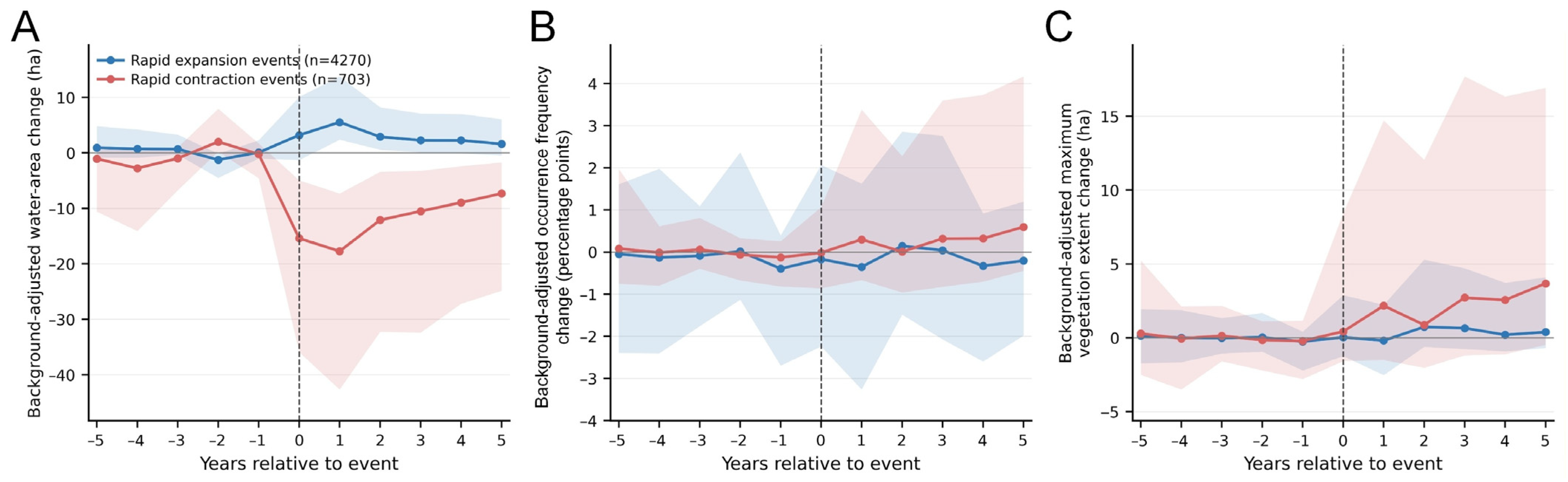
Results showed that the detected lake-area events were followed by changes that generally persisted beyond the event year (Figure 9A). For rapid expansion events, the median background-adjusted water-area change was 3.20 ha in the event year and increased to 5.52 ha one year later. The median difference then declined gradually but remained positive at 1.60 ha five years after the event. Rapid contraction events produced a much larger response in the opposite direction. Median water-area change reached −15.41 ha in the event year and −17.74 ha in the following year, before partially recovering to −7.33 ha by year +5. The continued negative values indicate that many rapid contractions represented persistent reductions in lake area rather than short-lived annual fluctuations. However, the broad interquartile ranges, particularly for contraction events, also indicate substantial variation in event magnitude and persistence among lakes.

Aquatic vegetation responded differently to expansion and contraction events. Vegetation occurrence frequency showed little systematic change following rapid lake expansion: the median response remained close to zero throughout the post-event period, ranging from −0.35 percentage points in year +1 to 0.14 percentage points in year +2 (Figure 9B). Maximum mapped vegetation extent also showed only a weak and inconsistent response to expansion, with a median change of 0.04 ha in the event year, −0.19 ha in year +1, and 0.74 ha in year +2 (Figure 9C). The interquartile ranges crossed zero in all post-expansion years, suggesting that lake expansion did not produce a uniform aquatic vegetation response across the lake population.

In contrast, rapid lake contraction was followed by a gradual positive shift in both vegetation metrics. Median occurrence-frequency change was close to zero in the event year, reached 0.30 percentage points in year +1, and increased to 0.60 percentage points by year +5. Maximum mapped vegetation extent increased from 0.43 ha in the event year to 2.17 ha in year +1 and 3.68 ha in year +5. These median trajectories are consistent with vegetation establishment or expansion within newly exposed shallow-water or littoral areas following water-area loss. Nevertheless, the wide uncertainty envelopes continued to include negative responses for many lakes, indicating that this was not a universal outcome of lake contraction.

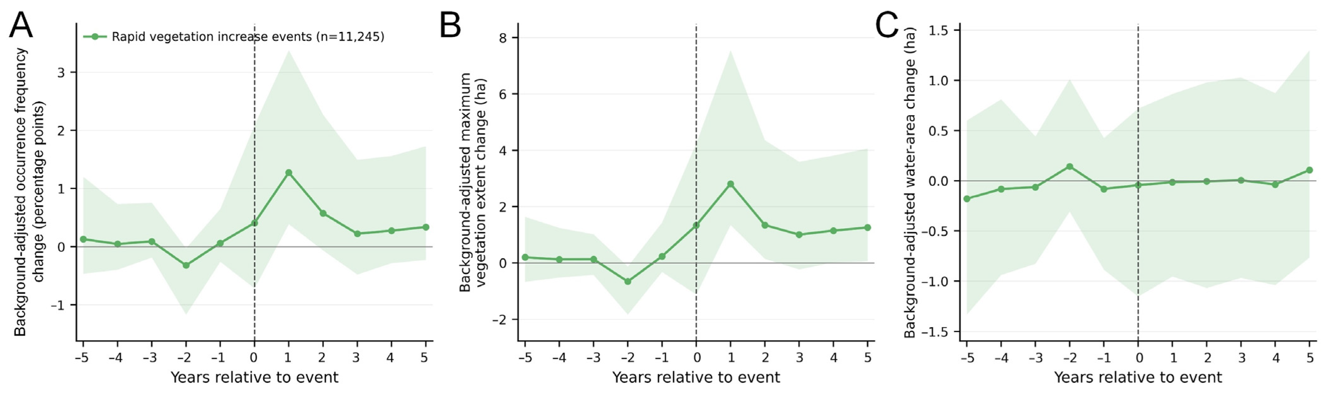
Rapid vegetation increase events exhibited a clearer event-centered pulse in both vegetation metrics (Figure 10A,B). The median background-adjusted occurrence frequency was 0.41 percentage points above the matched background in the event year and peaked at 1.27 percentage points in year +1. It subsequently declined but remained positive through year +5. Maximum mapped vegetation extent followed a similar trajectory, increasing by 1.33 ha in the event year and reaching 2.81 ha one year later. Median extent remained approximately 1.00–1.35 ha above the matched background during years +2 to +5. The concurrence of the two metrics confirms that these events represented both a larger annual vegetation footprint and more frequent vegetation detection.

Lake water area, however, showed no corresponding directional shift during vegetation increase events (Figure 10C). Median background-adjusted water-area change remained close to zero throughout the 11-year event window, including −0.04 ha in the event year, −0.02 ha in year +1, and 0.11 ha in year +5. This decoupling indicates that rapid increases in aquatic vegetation were generally not accompanied by abrupt changes in total lake water area. Vegetation increase events may therefore reflect changes occurring within existing lake boundaries, including colonization of shallow littoral zones, changes in inundation depth, and greater persistence of vegetation detection, rather than direct responses to simultaneous expansion or contraction of total lake water area.

Taken together, the event-scale results reinforce and further clarify the patterns identified by the long-term coupling analysis. Rapid lake contraction was followed by more consistent increases in both vegetation occurrence frequency and maximum mapped extent than rapid lake expansion, suggesting that water-level decline and the associated development of shallow or newly exposed littoral environments may provide favorable conditions for aquatic vegetation establishment. By contrast, rapid vegetation increase events generally occurred without a corresponding directional change in total lake water area. This indicates that short-term aquatic greening can develop through internal changes within lakes, such as redistribution of vegetation toward shallow margins or increased persistence within previously vegetated areas, without requiring substantial movement of the lake boundary. The relationship between water-area and vegetation dynamics therefore appears asymmetric: lake contraction may facilitate vegetation expansion in some lakes, whereas vegetation increases do not necessarily depend on abrupt water-area change.

3.5. Climate Conditions Associated with Rapid Aquatic Vegetation Increase Events

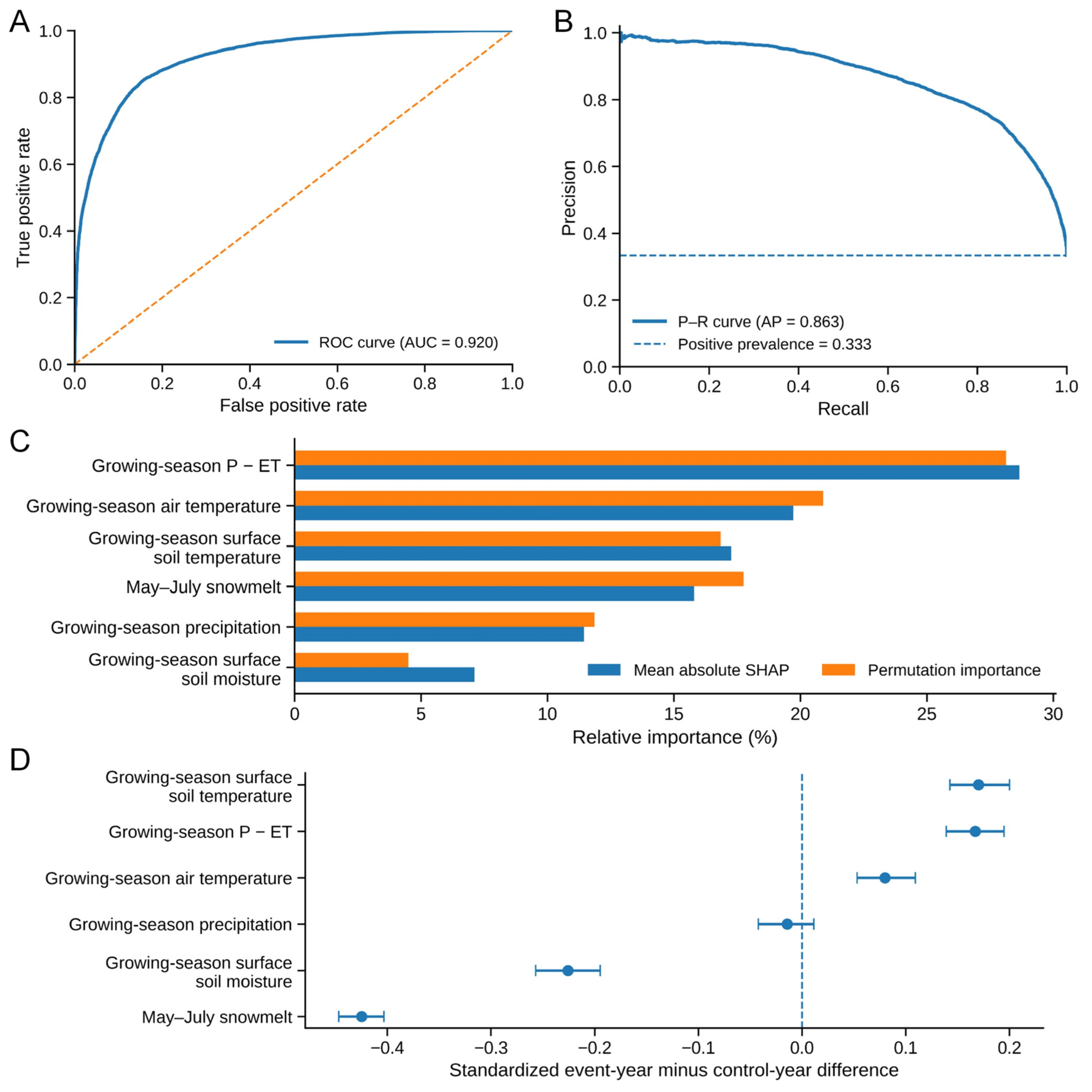
The CatBoost classifier distinguished rapid aquatic vegetation increase events from matched non-event years with high accuracy (Figure 11A,B). Under five-fold cross-validation grouped by lake ID, the model achieved a receiver operating characteristic area under the curve (ROC–AUC) of 0.920, with a bootstrap 95% confidence interval of 0.916–0.924. Average precision was 0.863, substantially exceeding the event prevalence of 0.333 in the matched dataset. At a classification threshold of 0.5, balanced accuracy was 0.845, sensitivity was 0.829, specificity was 0.861, precision was 0.749, and the F1 score was 0.787. A model based on the original climate values produced a lower ROC–AUC of 0.862, indicating that deviations from local long-term climate conditions were more informative than the absolute spatial climate gradients. Model performance remained high when observations sharing identical ERA5-Land climate values in the same year were assigned to the same validation group, yielding a ROC–AUC of 0.910.

Growing-season P−ET was the highest-ranked predictor within the fitted CatBoost model (Figure 11C), accounting for 28.7% of total mean absolute SHAP importance and 28.1% of permutation importance. Growing-season air temperature ranked second, while surface-soil temperature and May–July snowmelt had intermediate importance and precipitation and surface-soil moisture ranked lower. These percentages describe relative importance within this model. They should not be interpreted as ecological contribution fractions, particularly because air and soil temperature were strongly correlated and precipitation shared substantial information with precipitation minus evapotranspiration. The similar SHAP and permutation rankings are therefore treated as within-model consistency, not as independent evidence of robustness.

Direct comparisons between event and control years showed that rapid vegetation increase events occurred under a combination of wetter growing-season water balance, reduced May–July snowmelt, and altered near-surface thermal and moisture conditions (Figure 11D). The largest standardized difference was observed for snowmelt, which was substantially lower during event years than during matched non-event years (standardized difference = −0.425). Mean May–July snowmelt was 15.02 mm lower during event years. Growing-season P−ET showed a positive standardized difference of 0.167 and was, on average, 5.36 mm higher during event years. Surface-soil temperature also showed a positive standardized difference of 0.170, whereas surface-soil moisture was lower during event years, with a standardized difference of −0.226. Differences in total precipitation were comparatively small, indicating that the effective balance between water supply and atmospheric water loss was more informative than precipitation alone. The positive P−ET anomaly and lower surface-soil moisture are not necessarily contradictory: P−ET is a seasonal atmospheric water-balance measure, whereas near-surface soil moisture also reflects antecedent storage, drainage, thaw state, and local redistribution. The two variables therefore need not change in the same direction at the lake-centroid scale.

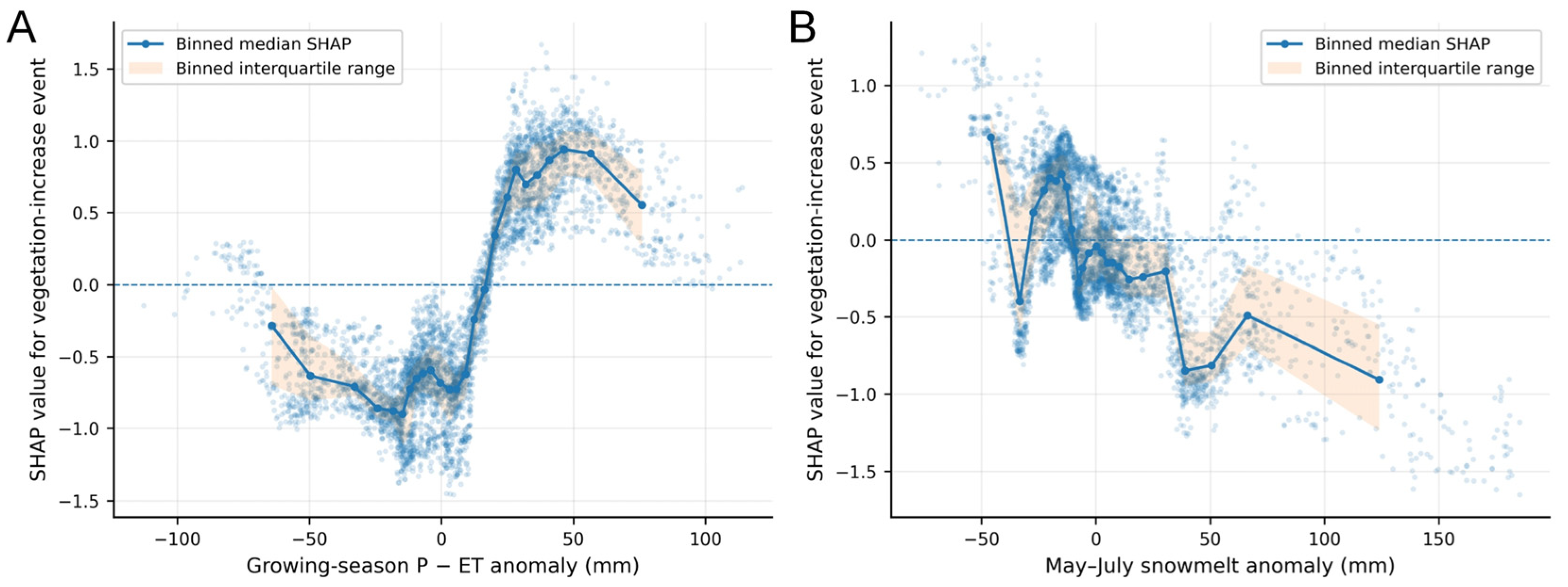
The SHAP dependence relationships further revealed that the climatic associations were nonlinear (Figure 12). Growing-season P−ET anomalies below approximately 10–15 mm generally reduced the predicted probability of a vegetation increase event, whereas positive anomalies above approximately 15–20 mm produced increasingly positive SHAP values (Figure 12A). The response reached its highest level under moderately positive water-balance anomalies and weakened slightly at the wettest end of the observed range. This pattern suggests that rapid aquatic vegetation increase was more likely during years with a positive growing-season moisture balance relative to local background conditions, but that the response was not proportional across the entire gradient.

May–July snowmelt showed an opposing model response (Figure 12B). Negative snowmelt anomalies generally produced positive SHAP values, while large positive anomalies reduced the predicted event probability. The paired comparison likewise showed lower May–July snowmelt during event years. Because ERA5-Land cumulative snowmelt does not resolve the timing of melt, we interpret this result only as an association with lower early-season melt totals and do not infer earlier snowmelt directly.

Air temperature and surface-soil-temperature anomalies were also important to model classification, but neither displayed a simple monotonic relationship with event occurrence. The two variables were highly correlated and therefore represented a shared thermal signal rather than fully independent controls. Their paired event–control differences were also less consistent than those of water balance and snowmelt. Consequently, the model results do not support a simple interpretation that warmer years universally promoted rapid aquatic vegetation increase. Instead, events were associated with particular combinations of thermal, water-balance, snowmelt, and soil-moisture conditions.

Although the model performed well when lakes were separated between training and validation folds, temporal transferability was limited. Leave-one-calendar-year-out validation produced a pooled ROC–AUC of 0.536 and average precision of 0.392, with held-out-year ROC–AUC values ranging from 0.286 to 0.736. Thus, the climate model distinguishes event and control observations well when training and validation data share the same calendar years, but the learned relationships do not generalize reliably to unseen years. The SHAP rankings and response curves are therefore interpreted as descriptive patterns in the pooled matched dataset, not as stable climatic drivers or transferable thresholds.

4. Discussion

4.1. Scale Compensation Behind Regional Water-Area Stability

The negligible net change in regional lake area should not be interpreted as hydrological stability. It resulted from compensation among lake size classes: gains distributed across numerous small lakes were offset by losses concentrated in a much smaller number of large lakes. Previous work in Northeast Siberia has documented long-term thermokarst lake expansion in the Kolyma lowlands [29], while regional drainage mapping has shown that abrupt lake losses are also widespread but spatially uneven [30]. Similar scale dependence is evident in broader lake inventories, where small lakes dominate changes in lake number while a limited set of large water bodies controls much of the total area signal [36]. Our results connect these two perspectives by showing that frequent small-lake expansion and less frequent large-lake losses can coexist within the same regional time series.

The greater prevalence of expansion among small lakes is consistent with their high shoreline-to-area ratios, shallow basins, and close contact with ice-rich margins, all of which increase their sensitivity to thaw settlement and shoreline erosion [29,36]. Larger lakes can lose substantial area through partial drainage, outlet development, or internal hydrological reorganization even when such events involve relatively few objects [21,24,32]. The present data do not resolve the mechanism of each individual change, but they show that a near-zero regional balance can coexist with widespread lake expansion and spatially concentrated but substantial lake-area losses. These opposing processes are unlikely to cancel biogeochemically: expansion inundates previously frozen or terrestrial substrates, whereas contraction exposes sediments and initiates a different sequence of carbon exchange and vegetation development [17,18,20,21,22].

The geographic pattern further indicates that regional means suppress meaningful environmental gradients. Expansion became more common toward the northern and coastal part of the study area, although latitude, coastal proximity, ground-ice conditions, and surface connectivity covary in this landscape. Assigning the pattern to a single control would therefore be premature. The observed pattern likely reflects interactions among lake size, geomorphic setting, and hydrological connectivity. Regional assessments based only on total surface water area may obscure this structural reorganization and may underestimate the importance of small lake expansion and large lake contraction for permafrost landscape change.

4.2. Aquatic Greening as Ecological Reorganization Within Lake Basins

The greatest change detected during 2000–2025 occurred in aquatic vegetation rather than in lake area. Maximum mapped vegetation extent increased across all lake size classes while regional water area remained almost unchanged. This pattern extends recent large-scale evidence from northern lakes [28] by showing that the increase was not confined to a regional total or a few dominant lakes. Nearly half of the analyzed lakes exhibited a significant increase in maximum extent, including many whose shorelines showed no directional change. Aquatic greening therefore represents an internal reorganization of thermokarst lake surfaces that cannot be inferred from open water area alone.

The contrast between maximum extent and occurrence frequency provides additional information about the form of this reorganization. Maximum extent increased by 172.5%, whereas the water area weighted occurrence frequency increased by 40.6%, and only about one tenth of the lakes showed a classified long-term increase in occurrence frequency. The expansion was therefore expressed more strongly as a larger annual vegetation footprint than as a uniform increase in the persistence of vegetation detection. Such a pattern is consistent with episodic occupation of shallow littoral areas during favorable years, shifts in seasonal phenology, or redistribution of vegetation within existing lake boundaries. It does not imply that the newly mapped area remained vegetated throughout the growing season or that biomass increased in direct proportion to mapped extent.

This distinction matters for both remote sensing and carbon assessment. Lake surfaces are often represented as a binary separation between open water and land, yet aquatic plants alter reflectance, sediment resuspension, organic matter accumulation, and pathways of methane transport [9,10,11,12,13,14,15]. The inclusion of aquatic vegetation has already been shown to raise northern lake methane estimates relative to calculations based on open water alone [10,28]. Although methane fluxes were not measured here, the magnitude and prevalence of the vegetation increase indicate that static open water classifications alone are insufficient to represent the changes observed within these lake basins. Future lake carbon assessments would benefit from representing biological cover, water depth, and hydrological state separately.

4.3. Asymmetric Coupling Between Lake Area and Aquatic Vegetation

The long-term and event-centered analyses converge on an asymmetric relationship between lake area and aquatic vegetation. Most increases in maximum vegetation extent occurred in lakes with stable or weakly changing water area, and rapid vegetation increase events were not accompanied by a directional shift in total lake area. Rapid contraction, however, was followed by a gradual increase in both vegetation metrics, whereas rapid expansion produced no consistent response. Aquatic vegetation can therefore respond to water loss in some lakes, but widespread aquatic greening does not require expansion or contraction of the mapped lake boundary.

The asymmetry is physically plausible because lake area is a two-dimensional measure that contains little information about water depth or the distribution of shallow habitat. Partial water loss can lower water levels, expose sediment, and widen shallow littoral zones without complete drainage. The positive response after contraction suggests that vegetation establishment can begin while part of the basin remains inundated, before the fully drained stage examined in previous studies [21,22,25,26,27]. The broad response ranges show that this pathway is not universal; shoreline slope, bathymetry, substrate, water clarity, and the persistence of the hydrological change will determine whether contraction creates suitable habitat or simply reduces the aquatic zone.

Lake expansion produced no consistent vegetation response. An increase in lake area may create new shallow margins, but it may also result from deeper inundation, active shoreline erosion, higher turbidity, or disturbance of established vegetation. The net vegetation response will depend on which of these processes dominates locally. Conversely, rapid greening under stable lake area can arise from changes in depth, phenology, nutrient availability, or optical conditions within an unchanged boundary. Aquatic vegetation may itself stabilize sediment and modify water optics [9,13,14,15], but the observational design cannot establish whether such feedbacks subsequently influence mapped water area. The term decoupling in this study therefore denotes partial independence between two observable dimensions of lake change, not an absence of hydrological influence on vegetation. Separating long-term trajectories from discrete events is essential for revealing this distinction.

4.4. Climate Associations, Uncertainty, and Future Research

Rapid vegetation increase events were associated with departures from the usual climate at each lake rather than with absolute regional climate gradients. Positive growing-season precipitation minus evapotranspiration and reduced May to July snowmelt were more informative than precipitation alone, while air and soil temperature showed nonlinear and partly redundant contributions. The results support a hydroclimatic interpretation in which seasonal water balance and snow conditions may influence whether a year is favorable for rapid vegetation expansion. They do not support a simple rule that warmer years consistently produce aquatic greening. This is consistent with the broader Arctic vegetation literature, which emphasizes that warming responses depend on moisture availability, seasonality, and local ecological constraints [5,8].

The contrast between the validation results places a clear limit on inference. The classifier separated event and control observations well when lakes were partitioned among folds, but performance declined to near-random when entire calendar years were withheld. The pooled record therefore contains recurring climate signatures of vegetation events, yet those signatures were not temporally stationary. Interannual differences in lake ice, water level, growing-season observations, regional hydrology, and unmeasured ecological conditions may alter the role of the selected predictors. The SHAP response curves should consequently be viewed as descriptive associations across the study period, not as transferable thresholds or evidence of causal climate control.

Several observational constraints remain. Landsat resolution limits detection along narrow shorelines and favors emergent and floating vegetation over submerged plants [13,14,15,28]. Occurrence frequency depends directly on the timing and number of valid observations, and maximum extent has a greater chance of capturing the seasonal peak in years with denser cloud-free coverage. Residual differences among Landsat sensors may also contribute to interannual variability despite common Collection 2 preprocessing and classification criteria. The fixed GLAKES envelope is useful for consistent object-based analysis, but it represents a multi-year maximum extent. The aquatic vegetation screening was designed to exclude dry terrestrial margins, yet mixed wetland or transitional pixels can still occur where formerly inundated margins become exposed. Conversely, expansion beyond the fixed envelope may be omitted. GLAD water area is a probability-weighted mapped water signal and can also be affected by dense vegetation. The event detector is therefore best viewed as a regional screening tool for abrupt annual shifts rather than an independently validated catalog of exact event dates; the centered smoothing introduces approximately ±1-year timing uncertainty. These limitations are why the main inference emphasizes repeated population-level patterns, matched controls, and multi-year contrasts rather than individual annual extremes or causal attribution.

Resolving these mechanisms requires observations that link shoreline movement to water depth and habitat conditions within lakes. Dynamic boundaries, higher resolution optical and radar imagery, satellite or field measurements of water level, and information on bathymetry and shoreline slope would help distinguish area change from depth change. Field surveys should separate aquatic plant functional types and quantify biomass, sediment conditions, and methane fluxes across stable, expanding, contracting, and drained lakes. Such measurements would test whether the associations identified here represent a sequence of hydroecological transitions and would allow aquatic vegetation dynamics to be incorporated more directly into assessments of permafrost lake carbon feedbacks.

5. Conclusions

Using 26 years of satellite observations and lake-object analyses, this study quantified long-term and event-scale changes in lake water area and aquatic vegetation across 32,439 thermokarst lakes in Northeast Siberia and examined the climate anomalies associated with rapid vegetation increases. The main conclusions are:

(1)

Regional lake water area changed by only 12.2 km² (0.05%) between 2000–2004 and 2021–2025 because gains in small lakes (197.9 km²) were largely offset by losses in large lakes (188.6 km²). Over the same period, maximum aquatic vegetation extent increased by 2057.2 km² (172.5%), while water-area-weighted occurrence frequency increased by 40.6%.

(2)

Aquatic greening was largely decoupled from long-term water area change. Maximum aquatic vegetation extent increased in 47.4% of lakes, and 39.9% of all lakes showed increasing vegetation under stable or weakly changing water area, compared with only 5.6% showing concurrent water expansion and vegetation increase.

(3)

The event responses were asymmetric. Five years after rapid lake contraction, median maximum vegetation extent and occurrence frequency had increased by 3.68 ha and 0.60 percentage points relative to matched controls, respectively. Rapid expansion produced no consistent vegetation response, while rapid vegetation increase events occurred with almost no corresponding water area change.

(4)

In the pooled matched dataset, rapid vegetation increase events were associated with wetter growing-season water balance and lower May–July snowmelt. Event years had 5.36 mm higher precipitation minus evapotranspiration and 15.02 mm less snowmelt than matched non-event years. However, leave-one-calendar-year-out performance was close to random (ROC–AUC = 0.536), so these climate relationships should be interpreted as pooled descriptive associations rather than stable or transferable climatic controls.

References

1. Miner, K.R.; Turetsky, M.R.; Malina, E.; Bartsch, A.; Tamminen, J.; McGuire, A.D.; Fix, A.; Sweeney, C.; Elder, C.D.; Miller, C.E. Permafrost Carbon Emissions in a Changing Arctic. Nat. Rev. Earth Environ. 2022, 3, 55–67. [Google Scholar] [CrossRef] [Scilit]
2. Rantanen, M.; Karpechko, A.Y.; Lipponen, A.; Nordling, K.; Hyvärinen, O.; Ruosteenoja, K.; Vihma, T.; Laaksonen, A. The Arctic Has Warmed Nearly Four Times Faster than the Globe since 1979. Commun. Earth Environ. 2022, 3, 168. [Google Scholar] [CrossRef] [Scilit]
3. Biskaborn, B.K.; Smith, S.L.; Noetzli, J.; Matthes, H.; Vieira, G.; Streletskiy, D.A.; Schoeneich, P.; Romanovsky, V.E.; Lewkowicz, A.G.; Abramov, A. Permafrost Is Warming at a Global Scale. Nat. Commun. 2019, 10, 264. [Google Scholar] [CrossRef] [Scilit] [PubMed]
4. Smith, S.L.; O’Neill, H.B.; Isaksen, K.; Noetzli, J.; Romanovsky, V.E. The Changing Thermal State of Permafrost. Nat. Rev. Earth Environ. 2022, 3, 10–23. [Google Scholar] [CrossRef] [Scilit]
5. Myers-Smith, I.H.; Kerby, J.T.; Phoenix, G.K.; Bjerke, J.W.; Epstein, H.E.; Assmann, J.J.; John, C.; Andreu-Hayles, L.; Angers-Blondin, S.; Beck, P.S.A. Complexity Revealed in the Greening of the Arctic. Nat. Clim. Change 2020, 10, 106–117. [Google Scholar] [CrossRef] [Scilit]
6. Frost, G.V.; Bhatt, U.S.; Macander, M.J.; Berner, L.T.; Walker, D.A.; Raynolds, M.K.; Magnússon, R.Í.; Bartsch, A.; Bjerke, J.W.; Epstein, H.E.; et al. The Changing Face of the Arctic: Four Decades of Greening and Implications for Tundra Ecosystems. Front. Environ. Sci. 2025, 13, 1525574. [Google Scholar] [CrossRef] [Scilit]
7. Heijmans, M.M.P.D.; Magnússon, R.Í.; Lara, M.J.; Frost, G.V.; Myers-Smith, I.H.; van Huissteden, J.; Jorgenson, M.T.; Fedorov, A.N.; Epstein, H.E.; Lawrence, D.M.; et al. Tundra Vegetation Change and Impacts on Permafrost. Nat. Rev. Earth Environ. 2022, 3, 68–84. [Google Scholar] [CrossRef] [Scilit]
8. Berner, L.T.; Massey, R.; Jantz, P.; Forbes, B.C.; Macias-Fauria, M.; Myers-Smith, I.H.; Kumpula, T.; Gauthier, G.; Andreu-Hayles, L.; Gaglioti, B.V. Summer Warming Explains Widespread but Not Uniform Greening in the Arctic Tundra Biome. Nat. Commun. 2020, 11, 4621. [Google Scholar] [CrossRef] [Scilit] [PubMed]
9. Song, Y.; Liew, J.H.; Sim, D.Z.H.; Mowe, M.A.D.; Mitrovic, S.M.; Tan, H.T.W.; Yeo, D.C.J. Effects of Macrophytes on Lake-Water Quality across Latitudes: A Meta-Analysis. Oikos 2019, 128, 468–481. [Google Scholar] [CrossRef] [Scilit]
10. Kyzivat, E.D.; Smith, L.C.; Garcia-Tigreros, F.; Huang, C.; Wang, C.; Langhorst, T.; Fayne, J.V.; Harlan, M.E.; Ishitsuka, Y.; Feng, D.; et al. The Importance of Lake Emergent Aquatic Vegetation for Estimating Arctic-boreal Methane Emissions. J. Geophys. Res. Biogeosciences 2022, 127, e2021JG006635. [Google Scholar] [CrossRef] [Scilit]
11. Bodmer, P.; Vroom, R.J.E.; Stepina, T.; del Giorgio, P.A.; Kosten, S. Methane Dynamics in Vegetated Habitats in Inland Waters: Quantification, Regulation, and Global Significance. Front. Water 2024, 5, 1332968. [Google Scholar] [CrossRef] [Scilit]
12. Elder, C.D.; Schweiger, M.; Lam, B.; Crook, E.D.; Xu, X.; Walker, J.; Walter Anthony, K.M.; Miller, C.E. Characterizing Methane Emission Hotspots from Thawing Permafrost. Glob. Biogeochem. Cycles 2021, 35, e2020GB006922. [Google Scholar] [CrossRef] [Scilit]
13. Wang, Y.; Gong, Z.; Zhou, H. Long-Term Monitoring and Phenological Analysis of Submerged Aquatic Vegetation in a Shallow Lake Using Time-Series Imagery. Ecol. Indic. 2023, 154, 110646. [Google Scholar] [CrossRef] [Scilit]
14. Wang, H.; Li, Y.; Zeng, S.; Cai, X.; Bi, S.; Liu, H.; Mu, M.; Dong, X.; Li, J.; Xu, J.; et al. Recognition of Aquatic Vegetation above Water Using Shortwave Infrared Baseline and Phenological Features. Ecol. Indic. 2022, 136, 108607. [Google Scholar] [CrossRef] [Scilit]
15. Dai, Y.; Feng, L.; Hou, X.; Tang, J. An Automatic Classification Algorithm for Submerged Aquatic Vegetation in Shallow Lakes Using Landsat Imagery. Remote Sens. Environ. 2021, 260, 112459. [Google Scholar] [CrossRef] [Scilit]
16. Piao, S.; Wang, X.; Park, T.; Chen, C.; Lian, X.; He, Y.; Bjerke, J.W.; Chen, A.; Ciais, P.; Tømmervik, H.; et al. Characteristics, Drivers and Feedbacks of Global Greening. Nat. Rev. Earth Environ. 2020, 1, 14–27. [Google Scholar] [CrossRef] [Scilit]
17. Turetsky, M.R.; Abbott, B.W.; Jones, M.C.; Walter Anthony, K.; Olefeldt, D.; Schuur, E.A.G.; Grosse, G.; Kuhry, P.; Hugelius, G.; Koven, C.; et al. Carbon Release through Abrupt Permafrost Thaw. Nat. Geosci. 2020, 13, 138–143. [Google Scholar] [CrossRef] [Scilit]
18. Schuur, E.A.G.; McGuire, A.D.; Schädel, C.; Grosse, G.; Harden, J.W.; Hayes, D.J.; Hugelius, G.; Koven, C.D.; Kuhry, P.; Lawrence, D.M.; et al. Climate Change and the Permafrost Carbon Feedback. Nature 2015, 520, 171–179. [Google Scholar] [CrossRef] [Scilit] [PubMed]
19. Natali, S.M.; Watts, J.D.; Rogers, B.M.; Potter, S.; Ludwig, S.M.; Selbmann, A.-K.; Sullivan, P.F.; Abbott, B.W.; Arndt, K.A.; Birch, L. Large Loss of CO2 in Winter Observed across the Northern Permafrost Region. Nat. Clim. Change 2019, 9, 852–857. [Google Scholar] [CrossRef] [Scilit] [PubMed]
20. Serikova, S.; Pokrovsky, O.S.; Laudon, H.; Krickov, I.V.; Lim, A.G.; Manasypov, R.M.; Karlsson, J. High Carbon Emissions from Thermokarst Lakes of Western Siberia. Nat. Commun. 2019, 10, 1552. [Google Scholar] [CrossRef] [Scilit] [PubMed]
21. Chen, Y.; Cheng, X.; Liu, A.; Chen, Q.; Wang, C. Tracking Lake Drainage Events and Drained Lake Basin Vegetation Dynamics across the Arctic. Nat. Commun. 2023, 14, 7359. [Google Scholar] [CrossRef] [Scilit] [PubMed]
22. Chen, Y.; Liu, A.; Cheng, X. Vegetation Grows More Luxuriantly in Arctic Permafrost Drained Lake Basins. Glob. Change Biol. 2021, 27, 5865–5876. [Google Scholar] [CrossRef] [Scilit] [PubMed]
23. Liu, A.; Cheng, X.; Wang, C.; Chen, Y. Evidence of Ecosystem Tipping Point on St. Lawrence Island: Widespread Lake Drainage Events after 2018. Geophys. Res. Lett. 2024, 51, e2024GL110161. [Google Scholar] [CrossRef] [Scilit]
24. Yang, X.; Liu, A.; Chen, Y. Divergent Spatiotemporal Patterns and Climate Responses of Lateral and Internal Lake Drainage in the Northern Permafrost Region. Geophys. Res. Lett. 2025, 52, e2025GL117233. [Google Scholar] [CrossRef] [Scilit]
25. Wolter, J.; Jones, B.M.; Fuchs, M.; Breen, A.; Bussmann, I.; Koch, B.P.; Lenz, J.; Myers-Smith, I.H.; Sachs, T.; Strauss, J.; et al. Post-Drainage Vegetation, Microtopography and Organic Matter in Arctic Drained Lake Basins. Environ. Res. Lett. 2024, 19, 045001. [Google Scholar] [CrossRef] [Scilit]
26. von Baeckmann, C.; Bartsch, A.; Bergstedt, H.; Efimova, A.; Widhalm, B.; Ehrich, D.; Kumpula, T.; Sokolov, A.; Abdulmanova, S. Land Cover Succession for Recently Drained Lakes in Permafrost on the Yamal Peninsula, Western Siberia. Cryosphere 2024, 18, 4703–4722. [Google Scholar] [CrossRef] [Scilit]
27. Liu, A.; Chen, Y.; Cheng, X. Effects of Thermokarst Lake Drainage on Localized Vegetation Greening in the Yamal–Gydan Tundra Ecoregion. Remote Sens. 2023, 15, 4561. [Google Scholar] [CrossRef] [Scilit]
28. Liu, J.; Huang, H.; Hou, X.; Feng, L.; Pi, X.; Kyzivat, E.D.; Zhang, Y.; Woodman, S.G.; Tang, L.; Cheng, X.; et al. Expansion of Aquatic Vegetation in Northern Lakes Amplified Methane Emissions. Nat. Geosci. 2025, 18, 322–329. [Google Scholar] [CrossRef] [Scilit]
29. Veremeeva, A.; Nitze, I.; Günther, F.; Grosse, G.; Rivkina, E. Geomorphological and Climatic Drivers of Thermokarst Lake Area Increase Trend (1999–2018) in the Kolyma Lowland Yedoma Region, North-Eastern Siberia. Remote Sens. 2021, 13, 178. [Google Scholar] [CrossRef] [Scilit]
30. Liu, A.; Chen, Y.; Cheng, X. Monitoring Thermokarst Lake Drainage Dynamics in Northeast Siberian Coastal Tundra. Remote Sens. 2023, 15, 4396. [Google Scholar] [CrossRef] [Scilit]
31. Olefeldt, D.; Goswami, S.; Grosse, G.; Hayes, D.; Hugelius, G.; Kuhry, P.; McGuire, A.D.; Romanovsky, V.E.; Sannel, A.B.K.; Schuur, E.A.G.; et al. Circumpolar Distribution and Carbon Storage of Thermokarst Landscapes. Nat. Commun. 2016, 7, 13043. [Google Scholar] [CrossRef] [Scilit] [PubMed]
32. Webb, E.E.; Liljedahl, A.K.; Cordeiro, J.A.; Loranty, M.M.; Witharana, C.; Lichstein, J.W. Permafrost Thaw Drives Surface Water Decline across Lake-Rich Regions of the Arctic. Nat. Clim. Change 2022, 12, 841–846. [Google Scholar] [CrossRef] [Scilit]
33. Nitze, I.; Cooley, S.W.; Duguay, C.R.; Jones, B.M.; Grosse, G. The Catastrophic Thermokarst Lake Drainage Events of 2018 in Northwestern Alaska: Fast-Forward into the Future. Cryosphere 2020, 14, 4279–4297. [Google Scholar] [CrossRef] [Scilit]
34. Chen, Y.; Liu, A.; Cheng, X. Landsat-Based Monitoring of Landscape Dynamics in Arctic Permafrost Region. J. Remote Sens. 2022, 2022, 9765087. [Google Scholar] [CrossRef] [Scilit]
35. Messager, M.L.; Lehner, B.; Grill, G.; Nedeva, I.; Schmitt, O. Estimating the Volume and Age of Water Stored in Global Lakes Using a Geo-Statistical Approach. Nat. Commun. 2016, 7, 13603. [Google Scholar] [CrossRef] [Scilit] [PubMed]
36. Pi, X.; Luo, Q.; Feng, L.; Xu, Y.; Tang, J.; Liang, X.; Ma, E.; Cheng, R.; Fensholt, R.; Brandt, M.; et al. Mapping Global Lake Dynamics Reveals the Emerging Roles of Small Lakes. Nat. Commun. 2022, 13, 5777. [Google Scholar] [CrossRef] [Scilit] [PubMed]
37. Pickens, A.H.; Hansen, M.C.; Hancher, M.; Stehman, S.V.; Tyukavina, A.; Potapov, P.; Marroquin, B.; Sherani, Z. Mapping and Sampling to Characterize Global Inland Water Dynamics from 1999 to 2018 with Full Landsat Time-Series. Remote Sens. Environ. 2020, 243, 111792. [Google Scholar] [CrossRef] [Scilit]
38. Pekel, J.-F.; Cottam, A.; Gorelick, N.; Belward, A.S. High-Resolution Mapping of Global Surface Water and Its Long-Term Changes. Nature 2016, 540, 418–422. [Google Scholar] [CrossRef] [Scilit] [PubMed]
39. Wulder, M.A.; Loveland, T.R.; Roy, D.P.; Crawford, C.J.; Masek, J.G.; Woodcock, C.E.; Allen, R.G.; Anderson, M.C.; Belward, A.S.; Cohen, W.B. Current Status of Landsat Program, Science, and Applications. Remote Sens. Environ. 2019, 225, 127–147. [Google Scholar] [CrossRef] [Scilit]
40. Zhu, Z.; Wulder, M.A.; Roy, D.P.; Woodcock, C.E.; Hansen, M.C.; Radeloff, V.C.; Healey, S.P.; Schaaf, C.; Hostert, P.; Strobl, P.; et al. Benefits of the Free and Open Landsat Data Policy. Remote Sens. Environ. 2019, 224, 382–385. [Google Scholar] [CrossRef] [Scilit]
41. Gorelick, N.; Hancher, M.; Dixon, M.; Ilyushchenko, S.; Thau, D.; Moore, R. Google Earth Engine: Planetary-Scale Geospatial Analysis for Everyone. Remote Sens. Environ. 2017, 202, 18–27. [Google Scholar] [CrossRef] [Scilit]
42. Tamiminia, H.; Salehi, B.; Mahdianpari, M.; Quackenbush, L.; Adeli, S.; Brisco, B. Google Earth Engine for Geo-Big Data Applications: A Meta-Analysis and Systematic Review. ISPRS J. Photogramm. Remote Sens. 2020, 164, 152–170. [Google Scholar] [CrossRef] [Scilit]
43. Muñoz-Sabater, J.; Dutra, E.; Agustí-Panareda, A.; Albergel, C.; Arduini, G.; Balsamo, G.; Boussetta, S.; Choulga, M.; Harrigan, S.; Hersbach, H.; et al. ERA5-Land: A State-of-the-Art Global Reanalysis Dataset for Land Applications. Earth Syst. Sci. Data 2021, 13, 4349–4383. [Google Scholar] [CrossRef] [Scilit]
44. Hersbach, H.; Bell, B.; Berrisford, P.; Hirahara, S.; Horányi, A.; Muñoz-Sabater, J.; Nicolas, J.; Peubey, C.; Radu, R.; Schepers, D. The ERA5 Global Reanalysis. Q. J. R. Meteorol. Soc. 2020, 146, 1999–2049. [Google Scholar] [CrossRef] [Scilit]
45. Hamed, K.H.; Rao, A.R. A Modified Mann–Kendall Trend Test for Autocorrelated Data. J. Hydrol. 1998, 204, 182–196. [Google Scholar] [CrossRef] [Scilit]
46. Sen, P.K. Estimates of the Regression Coefficient Based on Kendall’s Tau. J. Am. Stat. Assoc. 1968, 63, 1379–1389. [Google Scholar] [CrossRef]
47. Benjamini, Y.; Hochberg, Y. Controlling the False Discovery Rate: A Practical and Powerful Approach to Multiple Testing. J. R. Stat. Soc. Ser. B 1995, 57, 289–300. [Google Scholar] [CrossRef] [Scilit]
48. Kennedy, R.E.; Yang, Z.; Cohen, W.B. Detecting Trends in Forest Disturbance and Recovery Using Yearly Landsat Time Series: 1. LandTrendr—Temporal Segmentation Algorithms. Remote Sens. Environ. 2010, 114, 2897–2910. [Google Scholar] [CrossRef] [Scilit]
49. Chen, Y.; Liu, A.; Cheng, X. Detection of Thermokarst Lake Drainage Events in the Northern Alaska Permafrost Region. Sci. Total Environ. 2022, 807, 150828. [Google Scholar] [CrossRef] [Scilit] [PubMed]
50. Callaway, B.; Sant’Anna, P.H.C. Difference-in-Differences with Multiple Time Periods. J. Econom. 2021, 225, 200–230. [Google Scholar] [CrossRef] [Scilit]
51. Roth, J.; Sant’Anna, P.H.C.; Bilinski, A.; Poe, J. What’s Trending in Difference-in-Differences? A Synthesis of the Recent Econometrics Literature. J. Econom. 2023, 235, 2218–2244. [Google Scholar] [CrossRef] [Scilit]
52. Prokhorenkova, L.; Gusev, G.; Vorobev, A.; Dorogush, A.V.; Gulin, A. CatBoost: Unbiased Boosting with Categorical Features. In Proceedings of the 32nd International Conference on Neural Information Processing Systems (NIPS’18); Curran Associates Inc.: Red Hook, NY, USA, 2018; pp. 6639–6649. [Google Scholar]
53. Fisher, A.; Rudin, C.; Dominici, F. All Models Are Wrong, but Many Are Useful: Learning a Variable’s Importance by Studying an Entire Class of Prediction Models Simultaneously. J. Mach. Learn. Res. 2019, 20, 1–81. [Google Scholar]
54. Lundberg, S.M.; Erion, G.; Chen, H.; DeGrave, A.; Prutkin, J.M.; Nair, B.; Katz, R.; Himmelfarb, J.; Bansal, N.; Lee, S.-I. From Local Explanations to Global Understanding with Explainable AI for Trees. Nat. Mach. Intell. 2020, 2, 56–67. [Google Scholar] [CrossRef] [Scilit] [PubMed]
Figure 1. Location and land cover characteristics of the Northeast Siberian coastal tundra study area. (A) Circum-Arctic location of the study region. (B) Satellite map of the study area, showing the study area boundary and the distribution of the initial lake inventory. (C) Land cover composition within the study area.
Remotesensing 18 02898 g001
Figure 2. Overall workflow diagram of this study.
Remotesensing 18 02898 g002
Figure 3. Spatial distribution, size distribution, and size-class composition of lakes in the Northeast Siberian coastal tundra. (A) Spatial distribution of the analyzed lakes, colored by size class. (B) Frequency distribution of lake area on a logarithmic scale. (C) Relative contributions of small, medium, and large lakes to total lake number and total lake area.
Remotesensing 18 02898 g003
Figure 4. Size-dependent patterns of long-term lake water-area change in the Northeast Siberian coastal tundra. (A) Annual water area from 2000 to 2025, partitioned into small, medium, and large lakes. (B) Net change in mean water area between 2000–2004 and 2021–2025 for each lake-size class and for the regional total. (C) Proportions of lakes classified as expansion, stable or weak change, and contraction for all lakes and for each size class.
Remotesensing 18 02898 g004
Figure 5. Spatial and geographic patterns of long-term lake water-area trend classes in the Northeast Siberian coastal tundra. (A) Spatial distribution of lakes classified as expansion, stable or weak change, and contraction. (B) Longitudinal variation in the proportion of expanding and contracting lakes across 5° longitude bands. (C) Latitudinal variation in the proportion of expanding and contracting lakes across 1° latitude bands.
Remotesensing 18 02898 g005
Figure 6. Temporal changes in aquatic vegetation maximum extent and occurrence frequency in Northeast Siberian lakes from 2000 to 2025. (A) Annual regional maximum mapped aquatic vegetation extent, partitioned among small, medium, and large lakes. (B) Annual distribution of lake-scale aquatic vegetation occurrence frequency across all lakes. Boxes represent the interquartile range, horizontal lines indicate the median, whiskers extend from the 5th to the 95th percentile, and dots show the water-area-weighted mean. (C) Changes in mean annual maximum mapped aquatic vegetation extent between 2000–2004 and 2021–2025 for the regional total and the three lake-size classes. (D) Proportions of lakes classified as increasing, stable or weakly changing, and decreasing in long-term maximum aquatic vegetation extent. Regional maximum extent is the sum of lake-level annual maxima and does not represent a simultaneous regional vegetation map.
Remotesensing 18 02898 g006
Figure 7. Long-term coupling between lake water-area trends and maximum mapped aquatic vegetation extent in Northeast Siberian lakes from 2000 to 2025. (A) Lake-scale relationships between the Sen’s slopes of annual water area and maximum mapped aquatic vegetation extent. (B) Proportions of the six water-area–vegetation coupling classes for the total lake population and each lake-size class. (C) Spatial distribution of the six coupling classes. The vegetation stable category includes the very small number of lakes with decreasing maximum extent.
Remotesensing 18 02898 g007
Figure 8. Long-term coupling between lake water-area trends and aquatic vegetation occurrence frequency in Northeast Siberian lakes from 2000 to 2025. (A) Lake-scale relationships between the Sen’s slopes of annual water area and aquatic vegetation occurrence frequency. (B) Proportions of the six water-area–vegetation coupling classes for the total lake population and each lake-size class. (C) Spatial distribution of the six coupling classes. The vegetation stable category includes the very small number of lakes with decreasing maximum extent.
Remotesensing 18 02898 g008
Figure 9. Event-centered changes in lake water area and aquatic vegetation associated with rapid lake expansion and contraction events. (A) Background-adjusted lake water-area trajectories for rapid expansion events (n = 4270) and rapid contraction events (n = 703). (B) Corresponding changes in aquatic vegetation occurrence frequency. (C) Corresponding changes in maximum mapped aquatic vegetation extent. Solid lines show median responses, and shaded areas represent the interquartile range. The vertical dashed line denotes the event year (t = 0), and the horizontal line indicates no change relative to matched same-year and same-size non-event lakes.
Remotesensing 18 02898 g009
Figure 10. Event-centered changes in aquatic vegetation and lake water area associated with rapid vegetation increase events. (A) Background-adjusted changes in aquatic vegetation occurrence frequency during rapid vegetation increase events (n = 11,245). (B) Corresponding changes in maximum mapped aquatic vegetation extent. (C) Corresponding changes in lake water area. Solid lines show median responses, and shaded areas represent the interquartile range. The vertical dashed line denotes the event year (t = 0), and the horizontal line indicates no change relative to matched same-year and same-size non-event lakes.
Remotesensing 18 02898 g010
Figure 11. Predictive performance and relative importance of climatic conditions associated with rapid aquatic vegetation increase events. (A) Receiver operating characteristic curve for the CatBoost classifier evaluated using five-fold cross-validation. (B) Precision–recall curve; the dashed horizontal line represents the prevalence of vegetation increase events in the matched dataset. (C) Relative importance of the six climate predictors, quantified using SHAP values and permutation importance. (D) Standardized differences in climate anomalies between vegetation increase event years and matched non-event years from the same lakes. Points represent standardized mean differences, and error bars indicate 95% confidence intervals. Positive values indicate higher values during event years.
Remotesensing 18 02898 g011
Figure 12. Nonlinear associations of growing-season water balance and snowmelt anomalies with rapid aquatic vegetation increase events. (A) SHAP dependence relationship for growing-season precipitation minus evapotranspiration anomaly. (B) SHAP dependence relationship for May–July snowmelt anomaly. Points represent SHAP values for individual lake-year observations. Lines and shaded areas show the median and interquartile range of SHAP values within quantile-based bins, respectively. The horizontal dashed line indicates no contribution to the model prediction. Positive SHAP values indicate an increased predicted probability of a rapid aquatic vegetation increase event.
Remotesensing 18 02898 g012
Disclaimer/Publisher’s Note: The statements, opinions and data contained in all publications are solely those of the individual author(s) and contributor(s) and not of MDPI and/or the editor(s). MDPI and/or the editor(s) disclaim responsibility for any injury to people or property resulting from any ideas, methods, instructions or products referred to in the content.