SWH Retrieval from SWOT KaRIn Data by Combining Backscattering and Interference Characteristics

Highlights

What are the main findings?

• The proposed method integrating backscattering and interferometric features achieves favorable SWH retrieval accuracy. Compared with the operational KaRIn L2 SWH product, it reduces the RMSE by approximately 0.17 m, as validated against collocated ECMWF data.

What are the implications of the main findings?

• The retrieved SWH can be used to correct the sea state bias of sea surface height measurements obtained by the SWOT KaRIn, as well as to supplement wave products derived from other satellite sensors.

Abstract

This study focuses on the Significant Wave Height (SWH) retrieval from the Ka-band radar interferometer (KaRIn) on the Surface Water and Ocean Topography (SWOT) satellite by combining backscattering and interference characteristics. To this end, the backscattering-related and interference-related parameters were jointly used as inputs to develop a machine learning model. Here, the backscattering-related data include normalized radar cross-section (NRCS), incidence angle, and the image spectra parameters extracted from KaRIn Level 1B (L1B) data, while the interference-related data correspond to the Level 2 (L2) volumetric correlation, which characterizes the influence of ocean wave scattering on interferometric coherence. The machine learning model is built upon a Multi-Layer Perceptron (MLP), which serves as a nonlinear fitting tool. SWH retrievals from the proposed method and the existing L2 SWH product as a reference were validated by the collocated European Center for Medium-Range Weather Forecasts (ECMWF) reanalysis data, Haiyang2C (HY2C) and Haiyang2D (HY2D) altimeter data, and National Data Buoy Center (NDBC) buoy data. Validations show that both KaRIn SWH have a good agreement with collocations in terms of correlation coefficient (COR), BIAS and root mean square error (RMSE). Moreover, the retrieval accuracy from the proposed method (with an RMSE of about 0.29 m) is better than that of the L2 product (with an RMSE of about 0.46 m) when validated against the collocated ECMWF datasets. Ablation analysis further confirms that image spectra parameters and volumetric correlation are the dominant factors driving the retrieval accuracy improvement, with notable contribution differences among the sub-parameters of spectral features. This performance gain arises from the complementary physical mechanisms of backscattering and interferometric observables, which describe sea state information from independent dimensions. These accurate SWH retrievals can help correct sea state biases for collocated KaRIn sea surface height products and complement wave products from other satellite sensors.

1. Introduction

Significant Wave Height (SWH) is a crucial parameter for describing sea state in a variety of fields, including marine engineering, climate prediction, and maritime transportation [1]. SWH is defined as the mean height of the highest one-third of waves recorded at a specific location [2]. Traditionally, SWH has been acquired through buoy observations. Although buoy measurements offer high accuracy, they cannot achieve large-scale observations. With the advancements in satellite remote sensing technology, this limitation has been alleviated. Spaceborne radar has grown into a primary tool for obtaining global SWH data [3,4].

Common satellite radars for measuring SWH include traditional altimeters, wave spectrometers, and synthetic aperture radar (SAR) [5], each offering unique advantages for SWH retrieval [6]. Traditional altimeters are the most widely used due to their high accuracy and significant contribution to global SWH products. However, their swaths are limited, covering only areas near the nadir point [7]. In contrast, both wave spectrometers and SAR offer wider swaths, with SAR data providing a notably higher spatial resolution than wave spectrometers. Consequently, by combining the advantages of a wide swath and high spatial resolution, SAR has prompted many researchers to extract SWH from SAR imagery [8].

The methods for retrieving SWH from SAR imagery can be broadly categorized into two types: physically based [9] and empirical methods [10]. For physically based methods, nonlinear or quasilinear theoretical mapping relationships between image spectra and wave spectra are usually used. Due to the high wavenumber cutoff effects in the azimuth direction, the first guess spectrum is needed to compensate for the lost wave information. However, obtaining an accurate first guess spectrum and the inherent errors in theoretical relationships pose significant challenges for SAR wave spectra retrieval [11,12].

To alleviate the limitations of physically based methods, empirical models between SAR image parameters and wave information have been developed using data fitting techniques. For example, Schulz-Stellenfleth et al. proposed an empirical model known as CWAVE2.0 using ERS2 SAR data to estimate SWH with good accuracy [13]. However, developing a robust model still requires a significant amount of time and effort [14]. Recently, advancements in machine learning, such as deep learning, ensemble learning, and support vector machines, have provided new modeling approaches with high accuracy and efficiency. These data-driven methods have been applied to SAR data with satisfactory results [15,16].

In recent years, imaging radar altimeters have been developed for measuring sea surface height (SSH). Geometrically, it is similar to traditional SAR but operates at small incidence angles. Like traditional SAR, imaging altimeters have also shown the ability to retrieve SWH [17]. The Interferometric Imaging Radar Altimeter (InIRA) (in China’s Tiangong-2 space laboratory) is the first experimental spaceborne imaging radar. Considering the effectiveness of the empirical model in traditional SAR data, Ren et al. developed an empirical orthogonal model for SWH retrieval, using range and azimuth integration factors as input variables to extract SWH from InIRA data [18]. Despite the distinct backscattering mechanisms of InIRA (Quasi-specular) and SAR (Bragg scattering), both systems can get SWH retrievals with acceptable accuracy when employing empirical models [12,19].

On December 16, 2022, the National Aeronautics and Space Administration (NASA) successfully launched an operational imaging radar: the Ka-band radar interferometer (KaRIn) on the Surface Water and Ocean Topography Satellite (SWOT). KaRIn adopts a near-nadir angle (<4°) for interference measurement and has a wide swath (120 km) observation capability [20,21]. Preliminary SWH parameters have been included in the released Level 2 (L2) product [22]. This SWH is estimated from the volumetric coherence of the KaRIn interferogram. The estimation uses a least squares method applied to the normalized volumetric correlation and the inverse of the height sensitivity to phase [23,24,25,26]. Based on these studies, SWH is also directly retrieved from volumetric correlation data by an empirical model [27].

However, the currently released official KaRIn L2 SWH product is derived solely from the interferometric perspective, without incorporating backscattering-related observables that have been widely proven effective for sea state retrieval [18]. For traditional imaging radar systems such as SAR and interferometric imaging altimeters, backscattering-derived parameters including NRCS, incidence angle, and image spectra have long been verified to carry abundant sea state information and serve as core inputs for empirical SWH retrieval. Nevertheless, for the newly developed interferometric radar KaRIn, the potential value of these backscattering-related parameters has not been fully explored and integrated into the existing interference-based SWH retrieval scheme, which constitutes the main research gap addressed in this study.

Physically, backscattering-related parameters characterize sea surface roughness and wave energy distribution from the radar backscattering dimension, while volumetric correlation reflects the interferometric coherence attenuation induced by wave-driven volume scattering from the interference dimension. The two types of parameters respond to sea state variations through independent physical mechanisms and provide complementary sea state information. Therefore, integrating both categories of features can effectively compensate for the limitations of the single interference-based retrieval scheme, further improve retrieval accuracy, and reduce the incidence angle dependence of the existing product. Based on this consideration, this study will combine backscattering and interference characteristics of SWOT KaRIn data for improving the SWH retrieval accuracy. Due to the involvement of multiple parameters, this study uses a machine learning method to develop the model for its advantages in accuracy and computational efficiency.

The subsequent sections of the paper are organized as follows: Section 2 describes the materials and methods; Section 3 presents the results of validation and analysis; Section 4 discusses the results and limitations; and Section 5 provides a summary of the work.

2. Materials and Methods

2.1. Dataset

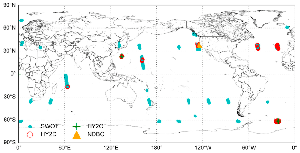
In this study, the data used include SWOT KaRIn Level 1B (L1B) and L2 data, and collocated European Center for Medium-Range Weather Forecasts (ECMWF) data, traditional Haiyang2C (HY2C) and Haiyang2D (HY2D) altimeter data, National Data Buoy Center (NDBC) buoy data, and Earth Topography 1 (ETOPO1) ocean depth data. The KaRIn and altimeter datasets are derived from satellite remote-sensing observations, ECMWF and ETOPO1 from numerical models, and NDBC datasets from in situ observations. ECMWF data were used as the primary reference for model training and validation, whereas the two altimeter datasets (HY2C and HY2D) and NDBC buoy data served as an independent benchmark to evaluate the retrieval results. Figure 1 illustrates the locations of SWOT KaRIn observations and collocated HY-2C, HY-2D, and NDBC buoy measurements. Below is a brief introduction to these data.

2.1.1. SWOT KaRIn

Currently, the released KaRIn dataset includes L1B, L2 and other products. Although these products are still in early stages, they have already demonstrated prominent ability in ocean surface topography observations, which are crucial for understanding and preserving ocean resources. In this study, the KaRIn L1B High-Rate Single-Look Complex (SLC) data and L2 Low-Rate product were used. A total of 4715 L1B data scenes were included in the analysis. The dataset covers both the calibration/validation phase and the early science phase, with a 1-day orbit repeat period in the calibration/validation phase and a 21-day repeat period in the science phase. The data acquisition time spans from January 2023 to 31 July 2023.

2.1.2. ECMWF

ECMWF is an international organization dedicated to global weather and climate forecasting. It uses advanced numerical models and extensive observational data to provide various types of meteorological and climatic information. ERA5 is ECMWF’s fifth-generation atmospheric reanalysis product and contains multiple datasets. This study chooses collocated SWH and rainfall data from hourly single-level ERA5 grid data through interpolation. Here, the spatial resolution of ERA5 data is 0.5° × 0.5° while the temporal resolution is 1 h. These data served as the collocations for model training and validation in this study.

2.1.3. HY2C and HY2D Altimeter

Owing to their well-validated accuracy, SWH measurements from traditional satellite altimeters are widely used as independent benchmarks for validating wave retrievals from new sensors. Accordingly, this study employs SWH data from the HY-2C and HY-2D altimeters to independently validate SWH retrievals derived from SWOT KaRIn observations. As the third and fourth satellites in the Haiyang-2 series, HY-2C and HY-2D were launched from the Jiuquan Satellite Launch Center, China. Similar to their predecessors Haiyang2A and Haiyang2B, they belong to China’s marine dynamic environment monitoring satellite series [28,29]. The HY-2C and HY-2D altimeter datasets used in this work were spatially and temporally matched with KaRIn data, with a temporal threshold less than 0.5 h and a spatial threshold within 5 km.

2.1.4. NDBC Buoy

The NDBC provides in situ wave observations, which serve as critical ground-truth references distinct from model outputs and satellite remote sensing data. In this study, NDBC buoy measurements are collocated with SWOT KaRIn observations using a temporal window of 0.5 h and a spatial threshold of 5 km. Detailed information for the selected collocated NDBC buoy stations is listed in

Table 1. Information of collocated NDBC buoy stations.

Buoy Name	Latitude (°/N)	Longitude (°/E)	Time (UTC)
46014	39.225	236.020	31 July 2023, 23:30
46214	37.937	236.537	31 July 2023, 23:30
46026	37.754	237.161	31 July 2023, 23:30

.

2.1.5. ETOPO1

ETOPO1 is a global elevation model providing topographic data on land and oceans with a 1-arcminute resolution, which is suitable for describing the features of the Earth’s surface and underwater terrain. It integrates elevation data from multiple sources in both the land and ocean regions to support scientific research and applications. This dataset is widely used in Earth science, climate modeling, and oceanography. Thus, ETOPO1 data are an important tool for studying global topography and marine landscapes. In this study, the ETOPO1 data were used to distinguish between land and ocean. Only bathymetric depths exceeding 50 m (i.e., elevation < −50 m) were considered [30].

2.2. Methods

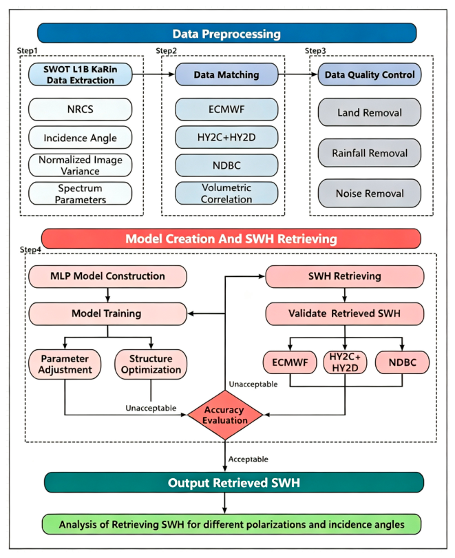
To improve the SWH retrieval accuracy, the backscattering and interference characteristics of SWOT KaRIn data were combined to develop a machine learning model. Figure 2 illustrates the flowchart of the proposed retrieval methodology. It consists of three key steps: model parameters, data preprocessing, and model development. The following subsections provide brief introductions to each step.

2.2.1. Model Parameters

In this work, the model parameters include two categories: backscattering-related (for backscattering characteristics) and interference-related (for interference characteristics) parameters. Here, the backscattering-related parameters include NRCS, incidence angle, normalized image variance and image spectra parameters, while the interference-related parameter is volumetric correlation from the KaRIn L2 product. The rationale for selecting these parameters is explained below.

(1)

NRCS and Incidence Angle

Numerous studies have demonstrated a strong correlation between NRCS and SWH. Chu et al. analyzed a decade of radar and collocated buoy data, verifying that virtually all sea state parameters are closely associated with the NRCS at low incidence angles [31]. Quilfen et al. also reported a good correlation between NRCS measurements and SWH [32]. As a metric for describing the reflectivity of extended targets or surfaces, NRCS is a useful parameter. Additionally, extensive measurements indicate that radar backscatter energy varies with the incidence angle. Furthermore, the quasi-specular reflection model (Equation (1)) [33] illustrates that NRCS is modulated by the incidence angle. Therefore, both NRCS and incidence angle were selected as model parameters in this study.

$${\sigma }_0={\displaystyle \frac{\left|\mathrm{R}\left(0\right)\right|}{{\overline{S}}^2}}{\sec }^4\theta \cdot \exp (-{\displaystyle \frac{{\tan }^2\theta }{{\overline{S}}^2}})$$

(1)

where θ is the incidence angle, R(0) is the Fresnel reflection coefficient at normal incidence, ${\mathrm{R}\left(0\right)}^2$ = 0.631, and ${\overline{S}}^2$ is the root mean square slope of the ocean surface.

(2)

Normalized Image Variance

Image variance is a statistical measure used to describe the variation in pixel values. Ocean waves can modulate the image variance through multiple modulation effects such as tilt modulation, hydrodynamic modulation, and velocity bunching modulation. Thus, a correlation exists between image variance and ocean wave parameters. Spatial variations in image variance can therefore be analyzed to infer ocean wave parameters. Hence, the normalized image variance (nv) was selected as a model parameter, calculated as follows:

$$nv=\mathrm{var}({\displaystyle \frac{I-〈I〉}{〈I〉}})$$

(2)

where I is the image intensity, $〈I〉$ is the mean value of I, and var represents the variance.

(3)

Image Spectra Parameters

The image spectra can be theoretically represented as the modulation of ocean wave spectra. So, it contains rich ocean wave information. However, if image spectra are directly introduced in the retrieval model, it will greatly increase the computational complexity. Therefore, this study replaces the use of spectra by extracting parameters from spectra using an orthonormal function. The extracted parameters can represent most of the spectral information and are easier to compute than directly using spectra. Specifically, the 20 image spectrum parameters refer to orthonormal expansion coefficients obtained by projecting the KaRIn image spectrum onto 20 predefined orthonormal basis functions. This parameterization scheme follows the classic empirical wave retrieval framework in Reference [10], and retains the dominant wave information while greatly reducing feature dimensions and computational complexity. Schulz et al. propose the CWAVE-ERS empirical algorithm [10], which uses a set of orthonormal functions to retrieve SWH by stepwise regression of 20 spectra parameters calculated from the variance spectra of SAR images. Ren et al. develop an empirical orthogonal SWH model using range and azimuth integration factors as model inputs to retrieve SWH from InIRA data, achieving an RMSE of less than 0.5 m, comparable to traditional SAR results [18]. We can see that the method using the orthonormal function has a good application for SWH retrieval [11,34,35]. Therefore, in this study, 20 spectra parameters estimated from the orthogonal function were selected as the input of the model. A complete description for parameter estimation is provided in [10].

(4)

KaRIn Volumetric Correlation

Many studies have demonstrated a distinct relationship between interferometric coherence and SWH [27]. The volumetric correlation, derived from interferograms, quantifies the coherence attenuation caused by vertical scattering effects within radar resolution cells—a phenomenon closely linked to ocean surface roughness and wave-induced elevation variations. Notably, volumetric correlation can directly and physically reflect the response of interference signals to changing sea states. Therefore, this study selects volumetric correlation as the interferometric parameter to extract SWH information from interference signals. Incorporating volumetric correlation introduces additional SWH-related information into the input parameters. In this study, the volumetric correlation used is a standard product included in the KaRIn Level-2 datasets. It has been resampled along the satellite orbit onto a geographically fixed 2 km × 2 km grid and is then spatially and temporally matched with other auxiliary parameters to ensure consistency for subsequent modeling and validation.

2.2.2. Data Preprocessing

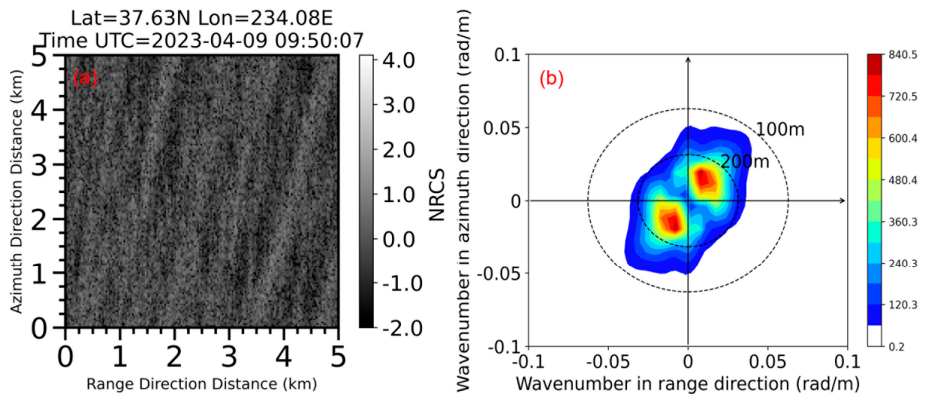
The model input parameters, except for KaRIn volumetric correlation, were first extracted from KaRIn L1B SLC data. Each SLC dataset was divided into 5 km × 5 km subimages for parameter extraction. As shown in Figure 3a, clear wave streaks can be observed in the subimage. Figure 3b presents the corresponding image spectra obtained by applying a Fourier transform to the subimage shown in Figure 3a. There is a slight truncation in the azimuth direction, which is a characteristic also observed in SAR systems. However, the spectral pattern remains largely intact, without sudden truncation at the spectral edge. This spectral characteristic indicates that KaRIn L1B SLC data retain sufficient wave spectral information and therefore exhibit strong potential for SWH retrieval. Then the NRCS, incidence angle, normalized image variance, and image spectra parameters were extracted from each subimage. These parameters were subsequently collocated in space and time with KaRIn volumetric correlation, ECMWF SWH data, and HY2C altimeter data, following the collocation criteria described in Section 2 (Dataset).

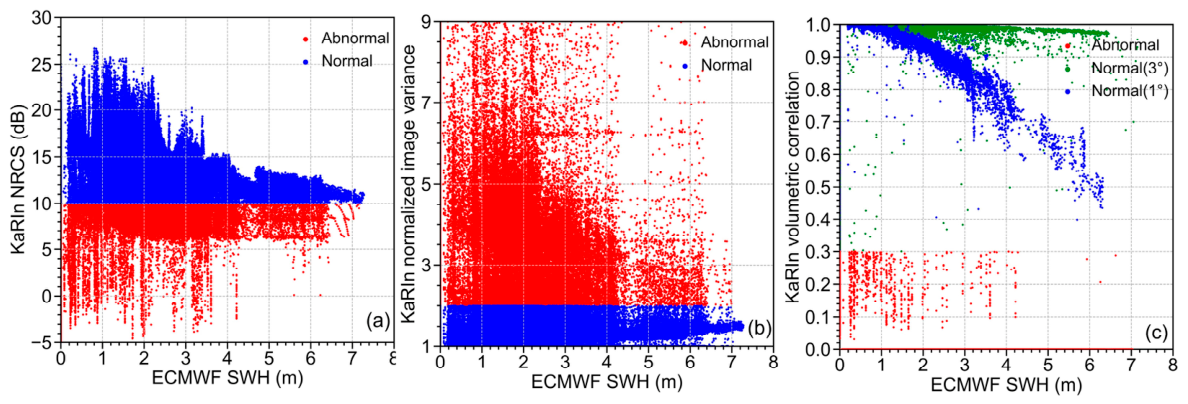
Subsequently, data quality control was applied. To minimize the influence of complex nearshore dynamics, data acquired over land or coastal regions with water depths shallower than 50 m were excluded using ETOPO1 bathymetric data. Furthermore, data affected by rainfall attenuation, identified based on ECMWF rainfall data, were also excluded. Moreover, considering the reasonable range of model input parameter values, additional data were excluded according to data distribution and previous studies [17,18,19,31,32]. Figure 4 shows the data distribution of NRCS, normalized image variance, and volumetric correlation along with the collocated SWH. Specifically, data with NRCS less than 10 dB, incidence angle outside the range of 0.5° to 4°, normalized image variance greater than 2, or volumetric correlation below 0.3 were discarded.

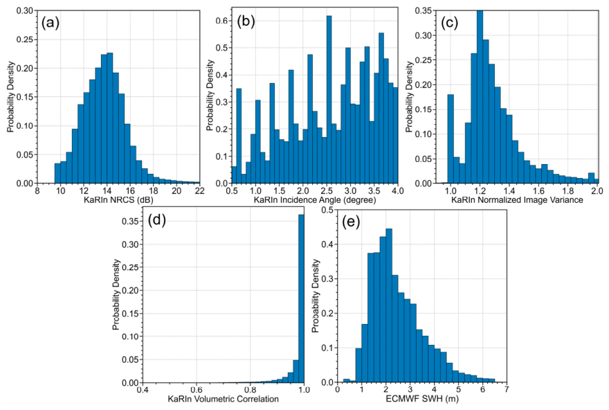
After quality control, approximately 199,000 collocated samples remain. Figure 5 shows the probability distribution of the data. As shown in the figure, NRCS (Figure 5a), normalized image variance (Figure 5c), and SWH (Figure 5e) basically follow a normal distribution, while the remaining two parameters (Figure 5b,d) exhibit a monotonically increasing trend. To ensure the independence of the modeling and validation processes, the dataset is divided into two parts: a training dataset and a validation dataset, with a ratio of 8:2, according to the satellite observation acquisition time. The training dataset is used to optimize the parameters of the machine learning model, while the validation dataset is used to evaluate the accuracy of KaRIn SWH retrieval.

2.2.3. Model Development

A Multi-Layer Perceptron (MLP) is a classical feed-forward neural network architecture that is widely used for nonlinear regression tasks [36]. Unlike recurrent neural networks, an MLP does not rely on temporal recurrence or sequential memory mechanisms. Instead, it learns a direct nonlinear mapping between a fixed-length input feature vector and the target variable through stacked fully connected layers. This structure is suitable for SWH retrieval because the relationship between KaRIn-derived observables, image spectral characteristics, and ocean wave parameters is highly nonlinear [37,38]. By combining multiple geophysical and image-derived features within a unified input vector, the MLP can effectively characterize the complex statistical relationship between SWOT Ka-RIn measurements and SWH.

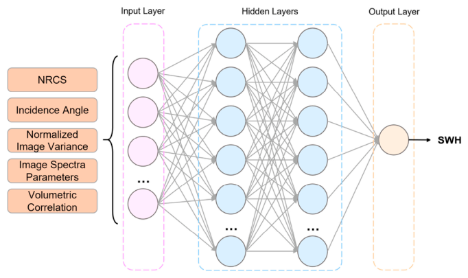
Therefore, an MLP-based model was constructed for SWH retrieval, as shown in Figure 6. The input layer contains 24 neurons corresponding to the 24 model input parameters, including NRCS, incidence angle, normalized image variance, 20 image spectrum parameters and volumetric correlation. Before being fed into the network, all input variables were standardized to reduce the influence of different feature scales on model training. The hidden part of the network consists of two fully connected layers. The first hidden layer maps the input features to 128 neurons, followed by a rectified linear unit (ReLU) activation function [39] and a dropout layer with a dropout rate of 0.3 [40]. The second hidden layer contains 64 neurons and is also followed by ReLU activation and dropout regularization. Finally, the output layer consists of a single neuron representing the estimated SWH. Through the use of nonlinear activation functions, the model is able to learn complex feature interactions, while dropout regularization helps reduce overfitting and improves the generalization ability of the network.

During model training, the collocated SWH data from the ECMWF ERA5 reanalysis product were used as the ground truth (training labels). The mean squared error (MSE) was used as the loss function, and the Adam optimizer was adopted to update the model parameters [41]. The initial learning rate was set to 0.0005. A total of 30 training epochs were conducted, with a batch size of 512 to balance computational efficiency and training stability. During training, the training loss and validation loss were recorded at each epoch, and the model with the lowest validation loss was saved for final evaluation.

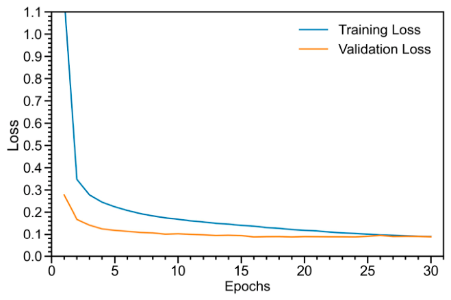
Figure 7 shows the training loss curve (labeled with a blue line). The training loss decreases sharply during the first few epochs, dropping from a relatively high initial value to approximately 0.3 within the early stage of training. Afterward, the loss continues to decline gradually and converges to around 0.09 by the end of the training process. The validation loss curve (labeled with an orange line) shows a similar decreasing trend, falling rapidly at the beginning and then stabilizing at a low level. Throughout most of the training process, the validation loss remains close to, and slightly lower than, the training loss, indicating that the model achieves stable convergence without evident overfitting. These results suggest that the MLP model effectively learns the nonlinear relationship between the input features and SWH, while maintaining good generalization performance on the validation dataset.

3. Results

3.1. Retrieval and Validation

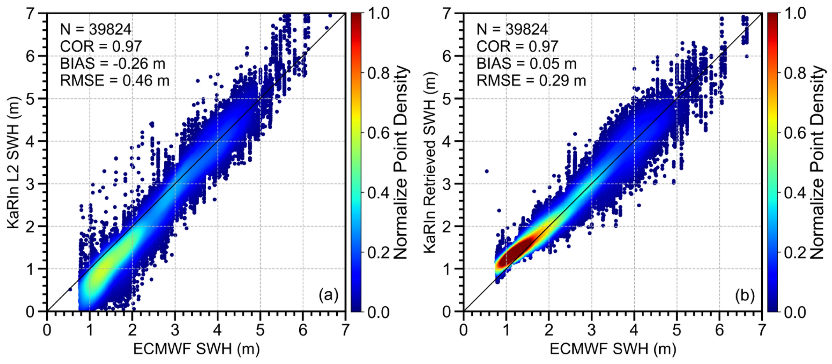
Following the development of the MLP-based model, SWH was retrieved by inputting the KaRIn parameters from the validation dataset, including NRCS, incidence angle, normalized image variance, image spectra parameters, and volumetric correlation. Then, the retrievals were validated against the collocated ECMWF, two altimeter SWH data and NDBC buoy data. Figure 8 shows the comparisons of KaRIn SWH with the collocated ECMWF data. In Figure 8a, the KaRIn SWH is from the released L2 product as a reference, while that in Figure 8b is from the retrievals of the proposed method. For the former, the correlation coefficient (COR) is 0.97, the BIAS is −0.26 m, and the root mean square error (RMSE) is 0.46 m; for the latter, the corresponding values are 0.97, 0.05 m, and 0.29 m, respectively. In both figures, most data points cluster near the reference line, indicating that both sets of KaRIn SWH data exhibit acceptable retrieval accuracy. It is noteworthy that the proposed method achieves better retrieval accuracy than the L2 product, with an RMSE reduction of 0.17 m. A paired t-test was conducted on the temporally independent validation set to test the statistical significance of this performance difference. The test yields a p-value < 0.001, confirming that the accuracy improvement of the proposed method is statistically significant.

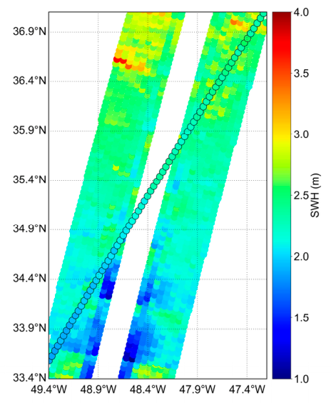
In addition to the ECMWF data, HY2C and HY2D altimeter SWH measurements were used as an independent dataset to validate the KaRIn SWH retrievals. Figure 9 shows an example of the spatial distribution of the KaRIn retrievals and the collocated HY2C altimeter data. As shown in the figure, the spatial variations in both datasets are consistent, with SWH gradually increasing from south to north.

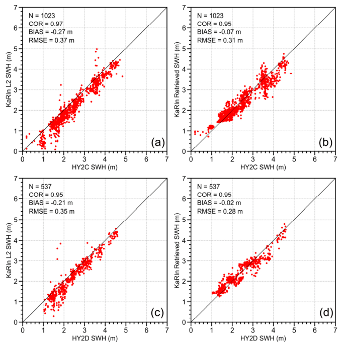
Moreover, Figure 10 compares the official KaRIn L2 SWH product and the retrievals from this study, with HY-2C and HY-2D altimeter data as independent validation benchmarks. The official L2 product exhibits good consistency with both altimeter datasets. For the HY-2C comparison (Figure 10a), the COR is 0.97, with a BIAS of −0.27 m and an RMSE of 0.37 m. For HY-2D (Figure 10c), the corresponding COR, BIAS and RMSE are 0.95, −0.21 m and 0.35 m, respectively. The proposed retrievals also maintain favorable agreement, with further improved accuracy. Validated against HY-2C (Figure 10b), they yield a COR of 0.95, a BIAS of −0.07 m, and an RMSE of 0.31 m. For HY-2D (Figure 10d), the COR stays at 0.95, with a BIAS of −0.02 m and an RMSE of 0.28 m. This method effectively reduces systematic bias and overall RMSE, confirming that the retrieval scheme combining backscattering and interference features outperforms the interference-only official product.

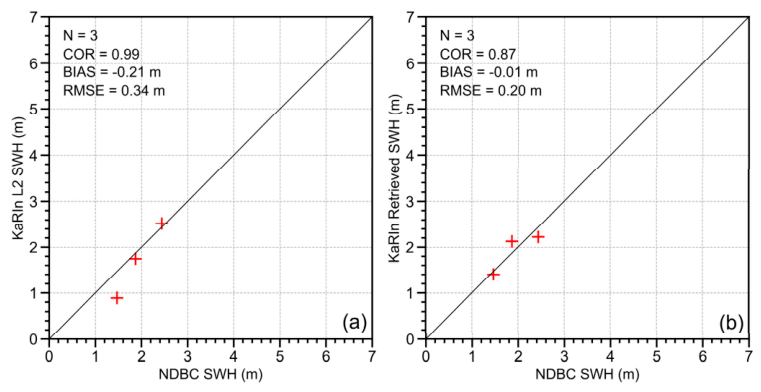
To further validate the retrieval results, NDBC in situ buoy measurements are employed as ground truth for comparison. For the official KaRIn L2 product (Figure 11a), the COR is 0.99, with a BIAS of −0.21 m and an RMSE of 0.34 m. For the retrievals from this study (Figure 11b), the COR is 0.87, with a BIAS of −0.01 m and an RMSE of 0.20 m. Owing to the limited collocated samples, these results are for reference only. The overall accuracy trend is consistent with the altimeter validation, and the proposed method yields lower systematic bias.

3.2. Ablation Analysis

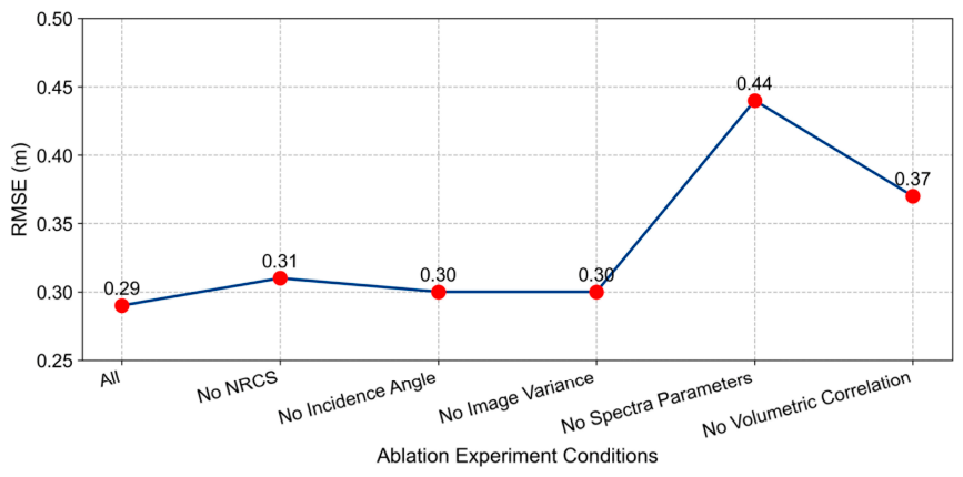
Ablation experiments were conducted to quantify the contribution of each input feature and verify the rationality of the model design. The full-feature model was taken as the baseline. Five ablation groups were constructed by removing one feature category separately, including NRCS, incidence angle, image variance, spectral parameters, and volumetric correlation. There were six experimental schemes in total. The importance of each feature was judged by the degree of RMSE deterioration after removal. The RMSE results of all schemes are shown in Figure 12. The full-feature model achieves the lowest RMSE of 0.29 m. Removing NRCS, incidence angle or image variance only causes slight RMSE increases, with values between 0.30 m and 0.31 m. These features have limited impact on retrieval accuracy. In comparison, removing spectra parameters leads to the most severe accuracy degradation, with RMSE rising to 0.44 m. This confirms that spectra parameters are the core factor affecting SWH retrieval performance. Removing volumetric correlation also results in an obvious RMSE increase to 0.37 m, reflecting its non-negligible effect. These results verify that the multi-feature fusion strategy effectively enhances model performance. Spectral parameters make the largest contribution to retrieval accuracy.

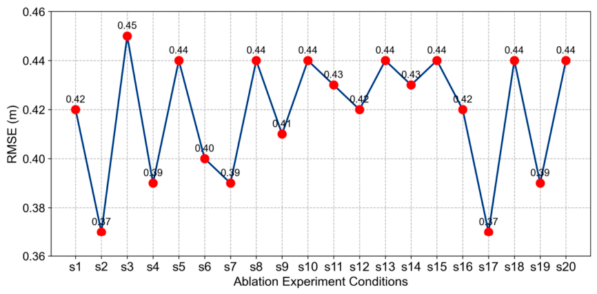
Given that spectral parameters make the largest contribution to SWH retrieval and contain 20 sub-parameters, further experiments were conducted to clarify the contribution difference in each parameter. All other non-spectral input features remained unchanged. Each test was constructed by adding only one spectral parameter to the model with all spectral features removed, forming 20 experimental schemes in total. The importance of each parameter was judged by the corresponding RMSE value: a lower RMSE indicates greater importance and contribution. As shown in Figure 13, the results show significant differences among the 20 spectral parameters, with RMSE values ranging from 0.37 m to 0.45 m. Parameters s2 and s17 achieve the lowest RMSE of 0.37 m, presenting the strongest contribution to retrieval accuracy. Parameter s3 yields the highest RMSE of 0.45 m with the weakest effect. Most parameters have RMSE between 0.39 m and 0.44 m, reflecting uneven importance within the spectra parameter set. The underlying reasons for such differences in parameter importance require further in-depth analysis.

3.3. Error Analysis

3.3.1. Error Variations with Radar Parameters

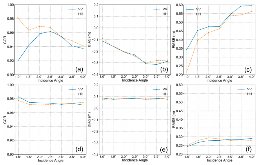
To further evaluate the robustness of the retrieval model, its performance under different polarization modes and incidence angles was analyzed. The dataset was first divided into vertical-vertical (VV) and horizontal-horizontal (HH) polarization subsets, and then grouped into incidence angle intervals of 0.5° for each polarization. Figure 14 illustrates the variations in COR, BIAS, and RMSE with incidence angle for both the KaRIn L2 product and the proposed retrievals under two polarizations. As shown in Figure 14a,d, both SWH products achieve high COR values across all polarization modes and incidence angles. For the official L2 product, the COR exhibits obvious incidence angle dependence: the HH polarization decreases from approximately 0.98 to 0.94 as incidence angle rises from 1.0° to 4.0°, while VV polarization first peaks at 0.96 around 2.5° and then declines slightly. In contrast, the proposed retrievals maintain consistently high COR values around 0.97 across all incidence angles, with negligible fluctuation for both polarizations. As shown in Figure 14b,e, the BIAS of the L2 product becomes increasingly negative with growing incidence angle, dropping from about −0.08 m to nearly −0.30 m. In comparison, the BIAS of the proposed retrievals remains stable near 0.05 m across the entire angle range, with almost no systematic drift. For RMSE (Figure 14c,f), the L2 product shows a pronounced increasing trend with incidence angle, rising by approximately 0.30 m from 1.0° to 4.0° for both polarizations. On the contrary, the RMSE of the proposed retrievals stays at 0.25–0.28 m with minimal variation, showing much weaker angle dependence. These comparisons confirm that the proposed model delivers reliable SWH retrieval performance. It not only outperforms the official L2 product in overall accuracy, but also maintains more stable performance across different polarizations and incidence angles.

3.3.2. Spatial Error Distribution

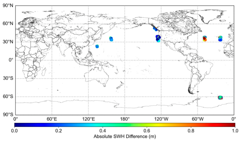
The spatial pattern of SWH retrieval errors was further investigated to evaluate the regional applicability of the proposed retrieval model. Figure 15 presents the global distribution of absolute SWH differences between the retrieved results and ECMWF reference data, where prominent error clusters are identified in four representative oceanic regions: the Northwest Pacific, Northeast Pacific, North Atlantic, and Southern Ocean.

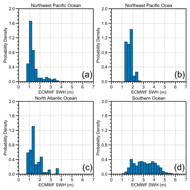
Detailed retrieval accuracy statistics for each region are summarized in

Table 2. Statistics for SWH retrieval validation across four ocean regions.

Region	N	COR	BIAS (m)	RMSE (m)
Northwest Pacific Ocean	10,296	0.9454	0.1414	0.2473
Northeast Pacific Ocean	2904	0.5223	−0.0217	0.2813
North Atlantic Ocean	4140	0.8402	0.2560	0.4394
Southern Ocean	22,442	0.8710	−0.0576	0.5252

. The Northwest Pacific Ocean achieves the best overall performance, with a COR of 0.9454, a BIAS of 0.1414 m, and an RMSE of 0.2473 m. The Northeast Pacific presents a relatively low correlation coefficient of 0.5223. This is mainly because the collocated samples in this region cover a narrow SWH range concentrated on small-to-moderate sea states. The correlation coefficient is inherently sensitive to the value span of the target variable; a limited SWH range naturally lowers the COR value, while its RMSE of 0.2813 m still indicates reliable absolute retrieval accuracy. In contrast, the Southern Ocean yields the largest RMSE of 0.5252 m. As revealed by the SWH probability density distributions in Figure 16, the Southern Ocean is characterized by generally higher wave heights and a wider distribution range, which is the dominant factor accounting for its elevated retrieval error magnitude.

To further evaluate the cross-regional generalizability of the retrieval model and verify whether the mapping relationship learned from local samples can be migrated to other sea areas, we conducted dedicated cross-region generalization experiments. Specifically, we trained the MLP model using only 80% of the samples from the Northwest Pacific Ocean as the training subset. The trained model was then tested on five independent datasets, including the remaining 20% of the Northwest Pacific samples (as the in-region performance baseline), the Northeast Pacific Ocean, the North Atlantic Ocean, the Southern Ocean, and the Indian Ocean. The detailed results are summarized in

Table 3. Cross-regional generalization performance of the regionally trained model, with the global model as the baseline reference.

Training Region	Test Region	N	COR	BIAS (m)	RMSE (m)
Northwest Pacific Ocean	Northwest Pacific Ocean	10,888	0.97	0.01	0.18
Northwest Pacific Ocean	Northeast Pacific Ocean	14,901	0.75	0.07	0.28
Northwest Pacific Ocean	North Atlantic Ocean	23,627	0.82	0.05	0.37
Northwest Pacific Ocean	Southern Ocean	91,052	0.91	−0.11	0.44
Northwest Pacific Ocean	Indian Ocean	5028	0.98	−0.02	0.31
Global model	All regions	39,824	0.97	0.05	0.29

.

The results reveal distinct performance characteristics of the regionally trained model. First, the model trained with Northwest Pacific samples achieves the highest accuracy on the in-region test set, with a COR of 0.97 and an RMSE of 0.18 m. This precision is superior to the overall performance of the global unified model (RMSE = 0.29 m), confirming that a region-customized model can deliver higher retrieval accuracy for specific target sea areas.

When migrated to other sea areas, the retrieval accuracy exhibits different degrees of decline. For the Northeast Pacific Ocean and the Indian Ocean, which have sea state ranges similar to the Northwest Pacific, the RMSE increases slightly to 0.28 m and 0.31 m, respectively, maintaining favorable retrieval performance. In contrast, for the North Atlantic Ocean and the Southern Ocean with wider SWH ranges and a higher proportion of high sea states, the RMSE rises obviously to 0.37 m and 0.44 m, respectively. The performance degradation is mainly attributed to the mismatch of sea state distribution: when the test sea states exceed the value range covered by the local training samples, the model’s nonlinear estimation ability is constrained.

In summary, the regionally trained model has higher application accuracy in the target sea area, but its global adaptability is insufficient. For global-scale applications such as satellite data calibration and global wave product generation, it is still necessary to construct the model with globally distributed samples covering diverse sea states, so as to ensure balanced and stable retrieval accuracy across all ocean regions.

4. Discussion

Besides wide-swath sea surface height measurements, SWOT KaRIn has the potential for measuring ocean waves owing to its high spatial resolution, similar to traditional SAR. Based on previous SAR studies [9,10], SWH can be retrieved from SAR images by physically based and empirical methods. The latter typically achieve higher retrieval accuracy owing to their superior ability to handle nonlinear relationships. Considering the effectiveness of the empirical model for SAR, this study also proposes an empirical machine learning model for retrieving KaRIn SWH. The validation results indicate that empirical models can also be successfully applied to the SWH retrieval from SWOT KaRIn data.

The preliminarily released KaRIn L2 products include SWH products. This SWH product is estimated only based on the interference coherence, which is a new attempt compared to previous studies [22,23,24,25]. However, in the commonly used SWH retrieval methods for SAR, backscattering-related parameters, such as NRCS, incidence angle, normalized image variance, and image spectra parameters, are usually used. To further improve the accuracy of KaRIn L2 products, this study combines backscattering-related parameters with the existing L2 SWH products, using them jointly as model inputs to retrieve SWH. Validation indicates that the SWH retrievals in this study have better accuracy than those of existing SWH products. The successful combined application of backscattering-related and interference-related parameters provides a new idea for retrieving ocean dynamic environmental parameters from interferometric radar in the future.

To clarify the contribution of each input feature and explore the underlying physical mechanism, two groups of ablation experiments were conducted. Feature-level ablation results show that image spectra parameters are the dominant contributor to retrieval accuracy. Volumetric correlation ranks as the second most impactful feature, while NRCS, incidence angle and image variance make relatively limited contributions. Further single-parameter ablation on spectral sub-parameters reveals that parameters s2 and s17 exert the strongest influence. Physically, image spectra parameters directly encode the energy distribution of ocean wave spectra, which has an intrinsic connection with significant wave height. Volumetric correlation reflects the interferometric coherence attenuation induced by wave-driven volume scattering, providing independent sea state information from the interferometric dimension. In contrast, individual parameters such as incidence angle and NRCS only reflect partial backscattering properties of the sea surface, thus contributing less to accuracy improvement.

For traditional SAR, polarization has a significant effect on data characteristics. VV-polarized data are more responsive to small-scale waves on the sea surface, while HH-polarized data can better capture the characteristics of large-scale waves. Therefore, different models are usually established for different polarizations. In this study, the SWH retrievals under different polarizations (VV and HH) were evaluated, and the accuracies are basically consistent for both polarizations. This indicates that the proposed model can simultaneously retrieve SWH for both polarizations, avoiding the need to establish separate models.

The accuracy of the existing L2 products degrades significantly with increasing incidence angles, primarily due to the attenuation of interferometric coherence. In contrast, the proposed method effectively minimizes this angular dependence by integrating multiple backscattering parameters, delivering stable retrievals across all incidence angles. Such angular independence ensures superior spatial consistency in the two-dimensional SWH field, thereby facilitating the detection and analysis of meso- and small-scale ocean surface phenomena.

The proposed shallow MLP model delivers reliable SWH retrieval performance. With two hidden layers of 128 and 64 neurons and approximately 11,500 trainable parameters, it achieves fast convergence and favorable computational efficiency under the current limited dataset. Its lightweight architecture holds great potential for on-board real-time retrieval on satellite platforms with strict computing and power constraints. The network structure can be further optimized to enhance scalability for large-scale long-term on-board applications.

One key limitation of this study is that training labels are derived from ECMWF reanalysis data, which transfers the numerical model’s inherent systematic biases to retrieval results and introduces a certain risk of self-validation. We introduced NDBC in situ buoy data as an independent validation benchmark, which qualitatively confirms the authenticity of the accuracy improvement. However, restricted by strict spatiotemporal matching criteria, valid collocated buoy samples are currently too few to quantitatively assess the exact magnitude of reanalysis-driven bias, requiring more independent in situ observations in follow-up work.

The model training data used in this study are mainly from sea states with SWH ranging from 1 to 7 m. Therefore, the proposed model may not be suitable for SWH values beyond 7 m. According to previous studies [42], the sea surface under typhoon conditions can generate extreme waves higher than 7 m. To extend the applicability of the model, it is necessary to collect more training data under high sea conditions. In the modeling process, attention should be paid to the stronger nonlinearities. In this case, other factors may need to be considered, such as the effect of wave breaking. Further experimental analysis similar to this study is also recommended to evaluate whether the developed model can perform well under high sea conditions

5. Conclusions

In this study, the backscattering and interference characteristics of SWOT KaRIn data are combined to develop a machine learning model for SWH retrieval. To this end, both backscattering-related and interference-related parameters are used simultaneously as inputs to construct a machine learning model. Here, the backscattering-related data include NRCS, incidence angle, and image spectra parameters extracted from KaRIn L1B data, while the interference-related data correspond to the volumetric correlation from the existing KaRIn L2 SWH product. The model is based on an MLP. The SWH retrievals from the proposed method and the L2 product are validated using collocated ECMWF, HY2C and HY2D altimeter, and NDBC buoy data. Validations show that both KaRIn SWH estimates agree well with the collocated references. More importantly, the retrieval accuracy of the proposed method is better than that of the existing L2 product. Moreover, retrieval performance was analyzed for two polarizations and across different incidence angles. Analysis shows that the retrieval accuracies for both KaRIn SWH products are stable across polarizations, while the proposed method exhibits greater independence from incidence angle compared to the L2 product.

Ablation results clarify the contribution hierarchy of input features: image spectra parameters dominate the retrieval accuracy, followed by volumetric correlation, while NRCS, incidence angle and normalized image variance contribute limitedly. Further analysis reveals notable heterogeneity among spectral sub-parameters, with s2 and s17 exerting the strongest influence. The accuracy improvement essentially arises from the complementary physical mechanisms: backscattering features characterize sea surface roughness and wave energy distribution, whereas volumetric correlation reflects wave-induced interferometric coherence attenuation, jointly providing multi-dimensional sea state information.

Regarding regional applicability, the locally trained model yields higher in-region accuracy but limited global adaptability. For global applications such as satellite calibration and operational wave products, globally distributed samples covering diverse sea states are required to ensure balanced performance. Cross-regional validation results demonstrate reasonable cross-regional transferability of the model, indicating that the learned mapping is not restricted to region-specific statistical features. These results demonstrate the feasibility of retrieving KaRIn SWH by combining backscattering and interference characteristics. The retrieved SWH data can help correct the sea state bias in collocated KaRIn sea surface height measurements and complement wave products from other sensors. The next step is to expand the retrieval capability of the method to high sea conditions

References

1. Stopa, J.; Cheung, K. Intercomparison of wind and wave data from the ECMWF reanalysis interim and the NCEP climate forecast system reanalysis. Ocean Model. 2014, 75, 65–83. [Google Scholar] [CrossRef] [Scilit]
2. Holthuijsen, L.H. Waves in Oceanic and Coastal Waters; Cambridge University Press: Cambridge, UK, 2007. [Google Scholar]
3. Liang, G.; Yang, J.; Wang, J. Accuracy evaluation of CFOSAT SWIM L2 products based on NDBC buoy and Jason-3 altimeter data. Remote Sens. 2021, 13, 887. [Google Scholar] [CrossRef] [Scilit]
4. Bué, I.; Lemos, G.; Semedo, Á. Assessment of satellite altimetry SWH measurements by in situ observations within 25 km from the coast. Ocean Dyn. 2024, 74, 183–210. [Google Scholar] [CrossRef] [Scilit]
5. Yang, Y.; Qi, J.; Yan, Q.; Fan, C.; Zhang, R.; Zhang, J. Reconstruction of wide swath significant wave height from quasi-synchronous observations of multisource satellite sensors. Earth Space Sci. 2024, 11, e2023EA003162. [Google Scholar] [CrossRef] [Scilit]
6. Adebisi, N.; Balogun, A.; Min, T.; Tella, A. Advances in estimating sea level rise: A review of tide gauge, satellite altimetry and spatial data science approaches. Ocean Coast. Manag. 2021, 208, 105632. [Google Scholar] [CrossRef] [Scilit]
7. Xu, J.; Wu, H.; Zhi, X.; Koldunov, N.V.; Zhang, X.; Xu, Y.; Zhang, Y.; Guo, M.; Kong, L.; Fraedrich, K. Validation of multisource altimeter SWH measurements for climate data analysis in China’s offshore waters. Remote Sens. 2024, 16, 2162. [Google Scholar] [CrossRef] [Scilit]
8. Schulz-Stellenfleth, J.; Lehner, S. Measurement of 2-D sea surface elevation fields using complex synthetic aperture radar data. IEEE Trans. Geosci. Remote Sens. 2004, 42, 1149–1160. [Google Scholar] [CrossRef]
9. Hasselmann, K.; Hasselmann, S. On the nonlinear mapping of an ocean wave spectrum into a synthetic aperture radar image spectrum and its retrieval. J. Geophys. Res. Ocean. 1991, 96, 10713–10729. [Google Scholar] [CrossRef] [Scilit]
10. Schulz-Stellenfleth, J.; König, T.; Lehner, S. An empirical approach for the retrieval of integral ocean wave parameters from synthetic aperture radar data. J. Geophys. Res. Ocean. 2007, 112, C03019. [Google Scholar] [CrossRef] [Scilit]
11. Sun, J.; Wang, X.; Yuan, X.Z.; Zhang, Q.J.; Guan, C.L.; Babanin, A.V. The dependence of sea SAR image distribution parameters on surface wave characteristics. Remote Sens. 2018, 10, 1843. [Google Scholar] [CrossRef] [Scilit]
12. Zhang, B.; Perrie, W. Recent progress on high wind-speed retrieval from multi-polarization SAR imagery: A review. Int. J. Remote Sens. 2014, 35, 4031–4045. [Google Scholar] [CrossRef] [Scilit]
13. Lehner, S.; Schulz-Stellenfleth, J.; Schattler, B.; Breit, H.; Horstmann, J. Wind and wave measurements using complex ERS-2 SAR wave mode data. IEEE Trans. Geosci. Remote Sens. 2000, 38, 2246–2257. [Google Scholar] [CrossRef] [Scilit]
14. Li, X.; Lehner, S.; Bruns, T. Ocean wave integral parameter measurements using ENVISAT ASAR wave mode data. IEEE Trans. Geosci. Remote Sens. 2011, 49, 155–174. [Google Scholar] [CrossRef] [Scilit]
15. Atteia, G.; Collins, M.; Algarni, A.; Samee, N. Deep-learning-based feature extraction approach for significant wave height prediction in SAR mode altimeter data. Remote Sens. 2022, 14, 5569. [Google Scholar] [CrossRef] [Scilit]
16. Xue, S.; Geng, X.; Yan, X.; Xie, T.; Yu, Q. Significant wave height retrieval from Sentinel-1 SAR imagery by convolutional neural network. J. Oceanogr. 2020, 76, 465–477. [Google Scholar] [CrossRef] [Scilit]
17. Yang, J.; Ren, L.; Zheng, G. The first quantitative ocean remote sensing by using Chinese interferometric imaging radar altimeter onboard TG-2. Acta Oceanol. Sin. 2017, 36, 122–123. [Google Scholar] [CrossRef] [Scilit]
18. Ren, L.; Yang, J.; Dong, X.; Jia, Y.; Zhang, Y. Preliminary significant wave height retrieval from interferometric imaging radar altimeter aboard the Chinese Tiangong-2 space laboratory. Remote Sens. 2021, 13, 2413. [Google Scholar] [CrossRef] [Scilit]
19. Li, G.; Zhang, Y.; Dong, X. Approaches for joint retrieval of wind speed and significant wave height and further improvement for Tiangong-2 interferometric imaging radar altimeter. Remote Sens. 2022, 14, 1930. [Google Scholar] [CrossRef] [Scilit]
20. Morrow, R.; Fu, L.; Ardhuin, F.; Benkiran, M.; Chapron, B. Global observations of fine-scale ocean surface topography with the Surface Water and Ocean Topography (SWOT) mission. Front. Mar. Sci. 2019, 6, 232. [Google Scholar] [CrossRef] [Scilit]
21. Neeck, S.P.; Lindstrom, E.J.; Vaze, P.V.; Fu, L.L. Surface water and ocean topography (SWOT) mission. In Proceedings of the Sensors, Systems, and Next-Generation Satellites XVI, Edinburgh, UK, 24–27 September 2012; Volume 8533, pp. 111–120. [Google Scholar] [CrossRef] [Scilit]
22. NASA JPL; CNES. SWOT Algorithm Theoretical Basis Document (Level-2 KaRIn Low Rate SSH); NASA JPL: Pasadena, CA, USA; CNES: Paris, France, 2023. [Google Scholar]
23. Peral, E.; Rodríguez, E.; Esteban-Fernández, D. Impact of surface waves on SWOT’s projected ocean accuracy. Remote Sens. 2015, 7, 14509–14529. [Google Scholar] [CrossRef] [Scilit]
24. NASA JPL; CNES. Mission Performance and Error Budget, Revision A; NASA JPL: Pasadena, CA, USA; CNES: Paris, France, 2017. [Google Scholar]
25. NASA JPL; CNES. SWOT Level-2 KaRIn Low Rate SSH Expert (V2.0); NASA JPL: Pasadena, CA, USA; CNES: Paris, France, 2023. [Google Scholar]
26. Bohé, A. Measuring significant wave height fields in two dimensions at kilometric scales with SWOT. IEEE Trans. Geosci. Remote Sens. 2025, 63, 1–19. [Google Scholar] [CrossRef] [Scilit]
27. Ren, L.; Dong, X.; Jia, Y.; Cui, L.; Zhang, Y.; Yang, J.; Wang, Y.; Jiang, Z. Significant wave height retrieval using the volumetric correlation data of SWOT. Geo-Spat. Inf. Sci. 2026, 29, 2026–2042. [Google Scholar] [CrossRef] [Scilit]
28. Qin, D.; Jia, Y.; Lin, M.; Liu, S. Performance evaluation of China’s first ocean dynamic environment satellite constellation. Remote Sens. 2023, 15, 4780. [Google Scholar] [CrossRef] [Scilit]
29. Wang, J.; Aouf, L.; Jia, Y.; Zhang, Y. Validation and calibration of significant wave height and wind speed retrievals from HY-2B altimeter based on deep learning. Remote Sens. 2020, 12, 2858. [Google Scholar] [CrossRef] [Scilit]
30. Amante, C.; Eakins, B. ETOPO1 Arc-Minute Global Relief Model: Procedures, Data Sources and Analysis; National Geophysical Data Center: Boulder, CO, USA; NOAA: Silver Spring, MD, USA, 2009. [Google Scholar]
31. Chu, X.; He, Y.; Karaev, V. Relationships between Ku-band radar backscatter and integrated wind and wave parameters at low incidence angles. IEEE Trans. Geosci. Remote Sens. 2012, 50, 4599–4609. [Google Scholar] [CrossRef] [Scilit]
32. Quilfen, Y.; Chapron, B.; Collard, F.; Vandemark, D. Relationship between ERS scatterometer measurements and integrated wind and wave parameters. J. Atmos. Ocean. Technol. 2004, 21, 368–373. [Google Scholar] [CrossRef] [Scilit]
33. Cox, C.; Munk, W. Measurement of the roughness of the sea surface from photographs of the sun’s glitter. J. Opt. Soc. Am. 1954, 44, 838–850. [Google Scholar] [CrossRef] [Scilit]
34. Wang, H.; Wang, J.; Yang, J.; Ren, L.; Zhu, J.; Yuan, X.; Xie, C. Empirical algorithm for significant wave height retrieval from wave mode data provided by the Chinese satellite Gaofen-3. Remote Sens. 2018, 10, 363. [Google Scholar] [CrossRef] [Scilit]
35. Dai, Z.; Li, H.; Wang, C.; He, Y. Backscattering statistics of labeled Sentinel-1 wave mode imagettes for ten geophysical phenomena. J. Mar. Sci. Eng. 2022, 10, 1594. [Google Scholar] [CrossRef] [Scilit]
36. Hornik, K.; Stinchcombe, M.; White, H. Multilayer feedforward networks are universal approximators. Neural Netw. 1989, 2, 359–366. [Google Scholar] [CrossRef] [Scilit]
37. Krasnopolsky, V.M. Neural network emulations for complex multidimensional geophysical mappings: Applications of neural network techniques to atmospheric and oceanic satellite retrievals and numerical modeling. Rev. Geophys. 2007, 45, RG3009. [Google Scholar] [CrossRef] [Scilit]
38. Vicen-Bueno, R.; Lido-Muela, C.; Nieto-Borge, J.C. Estimate of significant wave height from non-coherent marine radar images by multilayer perceptrons. EURASIP J. Adv. Signal Process. 2012, 2012, 84. [Google Scholar] [CrossRef] [Scilit]
39. Glorot, X.; Bordes, A.; Bengio, Y. Deep sparse rectifier neural networks. In Proceedings of the Fourteenth International Conference on Artificial Intelligence and Statistics, Fort Lauderdale, FL, USA, 11–13 April 2011; Volume 15, pp. 315–323. [Google Scholar]
40. Srivastava, N.; Hinton, G.; Krizhevsky, A.; Sutskever, I.; Salakhutdinov, R. Dropout: A simple way to prevent neural networks from overfitting. J. Mach. Learn. Res. 2014, 15, 1929–1958. [Google Scholar]
41. Kingma, D.P.; Ba, J. Adam: A method for stochastic optimization. In Proceedings of the International Conference on Learning Representations, San Diego, CA, USA, 7–9 May 2015. [Google Scholar]
42. Zhang, B.; Perrie, W. Remote sensing of tropical cyclones by spaceborne synthetic aperture radar: Past, present, and future. IEEE Geosci. Remote Sens. Mag. 2024, 12, 79–109. [Google Scholar] [CrossRef] [Scilit]
Figure 1. The spatial distribution of SWOT KaRIn and the collocated HY2C altimeter, HY2D altimeter and NDBC buoy data.
Remotesensing 18 02899 g001
Figure 2. Flowchart of SWH retrieval method proposed in this study.
Remotesensing 18 02899 g002
Figure 3. SWOT KaRIn L1B SLC data case. (a) NRCS data and (b) image spectra data extracted from (a).
Remotesensing 18 02899 g003
Figure 4. The SWOT KaRIn data distribution along with the collocated ECMWF SWH. (a) For NRCS, (b) for normalized image variance, and (c) for volumetric correlation at incidence angles of 1° and 3°. Here, the blue and green represent normal data, while the red represents abnormal data.
Remotesensing 18 02899 g004
Figure 5. Probability Density distribution after data quality control for (a) NRCS, (b) incidence angle, (c) normalized image variance, (d) volumetric correlation, and (e) ECMWF SWH.
Remotesensing 18 02899 g005
Figure 6. The MLP-based machine learning model structure for KaRIn SWH retrieval.
Remotesensing 18 02899 g006
Figure 7. The loss function of the MLP-based machine learning model.
Remotesensing 18 02899 g007
Figure 8. Comparisons of KaRIn SWH from (a) L2 product and (b) retrievals from the proposed method with the collocated ECMWF data.
Remotesensing 18 02899 g008
Figure 9. Spatial distribution comparisons between KaRIn SWH retrievals and collocated HY2C altimeter data. Here, the wide swath refers to KaRIn data, while the narrow swath is for HY2C altimeter data.
Remotesensing 18 02899 g009
Figure 10. Comparisons of KaRIn SWH: (a) KaRIn L2 product against collocated HY-2C altimeter data; (b) SWH retrieved by the proposed method against collocated HY-2C altimeter data; (c) KaRIn L2 product against collocated HY-2D altimeter data; (d) SWH retrieved by the proposed method against collocated HY-2D altimeter data.
Remotesensing 18 02899 g010
Figure 11. Comparisons of KaRIn SWH from (a) the L2 product and (b) retrievals from the proposed method with the collocated NDBC data.
Remotesensing 18 02899 g011
Figure 12. RMSE of SWH retrieval under different ablation experimental schemes.
Remotesensing 18 02899 g012
Figure 13. RMSE of SWH retrieval for individual spectra parameter experiments.
Remotesensing 18 02899 g013
Figure 14. Variation in KaRIn SWH retrieval accuracy with incidence angle. (a,d) show the correlation coefficient (COR); (b,e) show the bias (BIAS); (c,f) show the root mean square error (RMSE). The top row corresponds to the official L2 product, and the bottom row corresponds to the retrievals from the proposed method.
Remotesensing 18 02899 g014
Figure 15. Spatial distribution of absolute SWH difference between the retrievals and ECMWF reference data.
Remotesensing 18 02899 g015
Figure 16. Probability density distributions for different ocean regions: (a) Northwest Pacific Ocean; (b) Northeast Pacific Ocean; (c) North Atlantic Ocean; (d) Southern Ocean.
Remotesensing 18 02899 g016