Generalized Matérn Process for GNSS Coordinate Series Noise Modeling

Highlights

What are the main findings?

• A new generalized Matérn process (GMP) noise model was developed by introducing a fractional step size parameter μ, forming a unified noise model family that recovers the generalized Gauss–Markov (GGM) noise model at μ = 1 and approaches the spectral form of the Matérn process (MP) as μ → 0, while flexibly regulating spectral shape and autocovariance decay.
• Tests on 420 GNSS coordinate series identified a robust preferred range of μ ∈ [0.7, 1] with the strongest preference near μ = 0.90–0.95. In a global validation using 846 series, the WN + GMP family was selected for 88.9%, 37.5% and 50.1% of the series under AIC, BIC and BIC_tp, respectively.

What are the implications of the main findings?

• By embedding GGM and MP within a noise model family, GMP resolves ambiguities in their comparison and explicitly represents intermediate stochastic structures, thereby expanding the model space and improving the interpretability and fidelity of GNSS coordinate series noise modeling.
• The robust μ interval enables an efficient grid-based implementation for large GNSS networks. GMP preserves stable velocity estimates while providing a more flexible stochastic basis for assessing the model dependence of velocity uncertainties and supporting more defensible geodetic interpretations.

Abstract

GNSS coordinate series noise modeling is essential for reliable geophysical signal estimation and uncertainty assessment. The generalized Gauss–Markov (GGM) noise model and the Matérn process (MP) noise model are widely used to describe low-frequency spectral flattening in GNSS coordinate series, but they differ in their definition domains, parameterizations and autocovariance function (ACF) structures. These differences may lead to misconceptions, complicate noise model comparison and practical implementation. Building on a systematic review of the theories of GGM and MP, this study proposes a generalized Matérn process (GMP) noise model. By introducing a fractional step size hyperparameter μ into the differencing operator, GMP provides a unified framework that continuously connects the two models: when μ = 1, GMP reduces to GGM; as μ → 0, the spectrum of GMP approaches that of MP. The preferred range of μ is investigated using 420 GNSS coordinate series from 140 global GNSS sites, considering differences in geographical region, coordinate component and length of observations. The results show that the preferred values of μ are robustly concentrated within the interval [0.7, 1]. Large-scale validation is then conducted using 846 GNSS coordinate series from 282 global GNSS sites. The experimental results show that under AIC, BIC and BIC_tp, the proposed WN + GMP family consistently accounts for a large proportion of the optimal models. These results demonstrate that GMP provides a more general noise model family for GNSS coordinate series noise modeling and can improve the fidelity and flexibility of stochastic noise modeling.

1. Introduction

The GNSS coordinate series is a temporally ordered set of coordinates of a GNSS reference site, typically including the east, north and up components. GNSS coordinate series observations can be modeled by combining a functional model and a stochastic model: the functional model contains geophysical signals with clear physical meanings such as velocity, periodic terms, and offsets, whereas the stochastic model mainly represents unmodeled noise [1,2,3,4,5]. The geophysical signals in the functional model are widely used to study hot topics in the community of geosciences, such as crustal deformation, sea-level monitoring and terrestrial water storage inversion [6,7,8,9,10,11,12,13,14,15]. To obtain more accurate geophysical signals, researchers must investigate the mechanisms by which noise arises and model it effectively [16,17,18,19].

Since the 1990s, extensive research has been focused on noise modeling of GNSS coordinate series. Early studies assumed that GNSS coordinate series contained only pure white noise. However, this view was later shown to be incorrect because it ignores the temporal correlations [20]. Subsequent studies have shown that almost all GNSS coordinate series also contain various colored noise. Many studies have suggested that the combination of power-law noise and white noise (PL + WN) provides an appropriate stochastic model for a large proportion of GNSS coordinate series [18,21]. In recent years, with the accumulation of GNSS coordinate series data, long-period and low-frequency noise components have been increasingly detected. The power spectral density of GNSS series residuals exhibits a flattening pattern at low frequencies [22]. The generalized Gauss–Markov (GGM) noise model, proposed by Langbein in 2004, is well suited to characterizing this low-frequency spectral flattening behavior. Consequently, GGM has been widely used in GNSS coordinate series noise modeling [23,24,25,26]. In addition to GGM, the Matérn process (MP) noise model exhibits a similar spectral behavior—low-frequency flattening combined with power-law behavior at high frequencies—and is therefore also frequently used as a background noise model in Geoscience studies [27,28,29]. For example, the GNSS coordinate series analysis software Hector (version 2.1) provides both GGM and MP as candidate noise models for noise modeling.

Although GGM and MP are similar in spectrum, they differ in their discrete/continuous definition domains, parameterizations and autocovariance function structures. At present, the lack of a unified and systematic treatment of these two models has created obstacles for researchers when selecting noise models and interpreting parameter meanings in GNSS coordinate series noise modeling. In some studies, what is discussed as GGM is in fact MP or an equivalent form of MP [30,31,32]. Based on a systematic review of the theories of GGM and MP, this paper further proposes a new model family, the generalized Matérn process (GMP) noise model. The new GMP model introduces an additional fractional step-size parameter μ ∈ (0, 1] to unify and generalize the two existing noise models within a single framework: when μ = 1, GMP reduces to GGM; as μ → 0, GMP approaches the MP. The proposed GMP represents a much more general model family, significantly enriching the model library and further improving the modeling fidelity.

2. Methods

2.1. Generalized Gauss-Markov (GGM)

Assume that a discrete time series $\left\{x_t\right\}$ satisfies the following fractional-order difference equation [23]

$${\left(1-\varphi B\right)}^d{x}_t=w_t$$

(1)

In Equation (1), $\left\{w_t\right\}$ is a zero-mean Gaussian white noise series with variance ${\sigma }_w^2$. B denotes the backshift operator (B$x_t=x_{t-1}$). The GGM model has two noise parameters. One is the lag parameter ϕ ∈ (0, 1] which reflects the degree of correlation between adjacent observations. When ϕ = 1, the GGM reduces to a pure power-law process. The other is the spectral index d > 0, which reflects the long-term memory of the series. Applying a frequency-domain transformation to Equation (1), letting $\omega =2\pi f/f_s$ and using the correspondence $B\leftrightarrow e^{-j\omega }$, we obtain the transfer function:

$$H_{GGM}\left(\omega \right)={\displaystyle \frac{1}{{\left(1-\varphi e^{-j\omega }\right)}^d}}$$

(2)

Therefore, the power spectral density (PSD) of the GGM is given by

$$S_{GGM}\left(\omega \right)={\sigma }_w^2{\left|H_{GGM}\left(\omega \right)\right|}^2={\displaystyle \frac{{\sigma }_w^2}{{\left(1+{\varphi }^2-2\varphi \cos \omega \right)}^d}}$$

(3)

By applying the Gaussian hypergeometric function, a closed-form expression for the GGM autocovariance at lag i can be obtained:

$$R_{GGM}\left(i\right)={\sigma }_w^2{\displaystyle \frac{\mathsf{\Gamma }\left(d+i\right){\varphi }^i}{\mathsf{\Gamma }\left(d\right)\mathsf{\Gamma }\left(1+i\right)}}\times {}_{2}F_1\left(d+i;d;1+i;{\varphi }^2\right)$$

(4)

2.2. Matérn Process (MP)

Assume that a continuous-time process x(t) satisfies the following continuous-time differential equation [27,28]:

$${\left(\lambda +D\right)}^{d}x\left(t\right)=w\left(t\right)$$

(5)

In Equation (5), D denotes the differential operator $(\mathrm{D}{x}_t={\displaystyle \frac{\mathrm{d}}{\mathrm{dt}}}{x}_t)$ and $w\left(t\right)$ is a zero-mean Gaussian white-noise process. The Matérn process also has two noise parameters. One is the damping parameter λ > 0, for which λ → 0 yields a limiting form that approaches fractional Brownian motion. The other is the spectral index d $($typically $d>1/2)$, which typically characterizes the long-term memory of the process. To maintain consistency with the discrete time series $\left\{x_t\right\}$ in Section 2.1, we adopt the discrete sampling parameterization of the Matérn process given by [27]. Let $\omega =2\pi f$ and let the process variance be ${\sigma }^2$ then the corresponding power spectral density is given by

$$S_{MP}\left(\omega \right)={\displaystyle \frac{{\lambda }^{2d-1}}{C_d}}{\displaystyle \frac{{\sigma }^2}{{\left({\lambda }^2+{\omega }^2\right)}^d}}$$

(6)

In Equation (6), $C_d$ is the normalization constant, given by

$$C_d={\displaystyle \frac{1}{2\pi }}B\left({\displaystyle \frac{1}{2}},d-{\displaystyle \frac{1}{2}}\right)$$

(7)

In Equation (7), B denotes the beta function, $B\left(x,y\right)=\mathsf{\Gamma }\left(x\right)\mathsf{\Gamma }\left(y\right)/\mathsf{\Gamma }\left(x+y\right)$. By using the modified Bessel function of the second kind $K_v\left(·\right)$, a closed-form expression for the Matérn process autocovariance at lag i can be obtained:

$$R_{MP}\left(i\right)={\displaystyle \frac{2{\sigma }^2}{\mathsf{\Gamma }\left(d-\frac{1}{2}\right)2^{d-\frac{1}{2}}}}{\left|\lambda i\right|}^{d-{\displaystyle \frac{1}{2}}}{K}_{d-{\displaystyle \frac{1}{2}}}\left(\left|\lambda i\right|\right)$$

(8)

2.3. Generalized Matérn Process (GMP)

To place GGM and MP within a unified framework and introduce a mechanism to interpolate between them, we propose the generalized Matérn process (GMP). The key idea is to introduce a fractional step size parameter μ ∈ (0, 1] into the differencing operator. Consider a continuous-time function x(t); the fractional step size shift operator is defined as

$${\mathrm{B}}_{\mu }x\left(t\right)=x\left(t-\mu \right)$$

(9)

Introduce the following auxiliary parameters:

$$\zeta ={\displaystyle \frac{1}{1+\mu \lambda }}$$

(10)

The stochastic fractional difference equation with step size μ is

$${\left(1-\zeta {\mathrm{B}}_{\mu }\right)}^d\left[x\left(t\right)\right]={\left(\mu \zeta \right)}^{d}w\left(t\right)$$

(11)

In Equation (11), w(t) is a zero-mean Gaussian white-noise process. Using the correspondence $B_{\mu }\leftrightarrow e^{-j\mu \omega }$, the power spectral density of the GMP is given by

$$S_{GMP}\left(\omega \right)={\displaystyle \frac{{\sigma }^2{\left(\mu \zeta \right)}^{2d}}{{\left(1+{\zeta }^2-2\zeta \cos \left(\mu \omega \right)\right)}^d}}$$

(12)

To quantify the role of in controlling the spectral and temporal correlation characteristics of GMP, the denominator of Equation (12) can be rewritten as

$$1+{\zeta }^2-2\zeta \cos \left(\mu \omega \right)={\left(1-\zeta \right)}^2+4\zeta {\sin }^2\left(\mu \omega /2\right)$$

(13)

For the low-frequency regime, μω ≪ 1, the GMP spectrum can be approximated by

$$S_{GMP}\left(\omega \right)\approx {\displaystyle \frac{{\sigma }^2{\zeta }^d}{{\left({\omega }^2+{\lambda }^2\zeta \right)}^d}}$$

(14)

This expression defines an effective corner frequency,

$${\omega }_c=\lambda \sqrt{\xi }={\displaystyle \frac{\lambda }{\sqrt{1+\mu \lambda }}}$$

(15)

which quantitatively characterizes the transition from the low-frequency plateau to the power-law decay regime. Accordingly, the local logarithmic spectral slope can be approximated as:

$$\beta \left(\omega \right)=-{\displaystyle \frac{𝜕\ln S_{GMP}}{𝜕\ln \omega }}\approx {\displaystyle \frac{2d{\omega }^2}{{\omega }^2+{\omega }_c^2}}$$

(16)

Therefore, primarily controls the limiting spectral slope, whereas and jointly regulate the location of the spectral transition. For fixed λ, decreasing μ increases ωc, shifting the transition toward higher frequencies.

The same approximation also provides a quantitative interpretation in the time domain. Since a spectrum proportional to ${\left({\omega }^2+{\omega }_c^2\right)}^{-d}$ has a Matérn-type autocovariance whose large-lag behavior contains the exponential factor exp(−ωcτ), a characteristic correlation time can be defined as

$${\tau }_c={\displaystyle \frac{1}{{\omega }_c}}={\displaystyle \frac{\sqrt{1+\mu \lambda }}{\lambda }}$$

(17)

Thus, for fixed λ, a larger μ corresponds to a longer characteristic correlation time and slower ACF decay, whereas decreasing μ shortens the correlation time and produces a progressively more MP-like decay. These relationships provide a quantitative link between μ, spectral transition behavior, and temporal correlation duration. It should nevertheless be emphasized that μ acts jointly with λ and d, rather than serving as an independent physical descriptor of a specific GNSS noise source.

Because the GMP is defined with a continuous expression for the spectral form, when it is applied to discretely sampled daily GNSS coordinate series (sampling interval Δ = 1 day), the covariance at integer lags should be considered. In this study, the autocovariance function of the GMP is approximated using an FFT-based method; details are provided in Appendix A. Next, we verify how the GMP achieves endpoint consistency by tuning the parameter μ.

When μ = 1, the GMP reduces to the GGM. Let μ = 1, then $B_{\mu }=B$, $\zeta =1/\left(1+\lambda \right)$ and Equation (12) becomes

$${\left.S_{GMP}\left(\omega \right)\right|}_{\mu =1}={\displaystyle \frac{{\sigma }^2{\left(\zeta \right)}^{2d}}{{\left(1+{\zeta }^2-2\zeta \cos \omega \right)}^d}}$$

(18)

Comparing Equation (18) with Equation (3), the parameter mapping can be adjusted as follows:

$$\varphi =\zeta ={\displaystyle \frac{1}{1+\lambda }},\hspace{1em}\hspace{1em}{\sigma }_{GGM}^2={\sigma }_{GMP}^2{\zeta }^{2d}$$

(19)

One can see that

$${\left.S_{GMP}\left(\omega \right)\right|}_{\mu =1}=S_{GGM}\left(\omega \right)$$

(20)

Therefore, when μ = 1, the GMP is equivalent to the GGM under the parameter mapping ϕ = 1/(1 + λ).

When μ → 0, the GMP approaches the MP, then $\zeta =1/\left(1+\mu \lambda \right)\to 1$, one can obtain

$$1+{\zeta }^2-2\zeta \cos \mu \omega ={\mu }^2\left({\omega }^2+{\lambda }^2\right)+o\left({\mu }^2\right)$$

(21)

Substituting Equation (21) into Equation (12) and canceling ${\mu }^{2d}$ yields the following limit:

$$\underset{\mu \to 0}{\lim }{S}_{GMP}\left(\omega \right)={\displaystyle \frac{{\sigma }^2}{{\left({\omega }^2+{\lambda }^2\right)}^d}}$$

(22)

Compared with Equation (6), Equation (22) differs only by a constant factor; it therefore suffices to set

$${\sigma }_{GMP}^2={\sigma }_{MP}^2{\displaystyle \frac{C_d}{{\lambda }^{2d-1}}}$$

(23)

One can see that

$$\underset{\mu \to 0}{\lim }{S}_{GMP}\left(\omega \right)={\displaystyle \frac{{\lambda }^{2d-1}}{C_d}}{\displaystyle \frac{{\sigma }^2}{{\left({\omega }^2+{\lambda }^2\right)}^d}}=S_{MP}\left(\omega \right)$$

(24)

Therefore, as μ → 0, the spectrum of the GMP has the same shape as that of the MP.

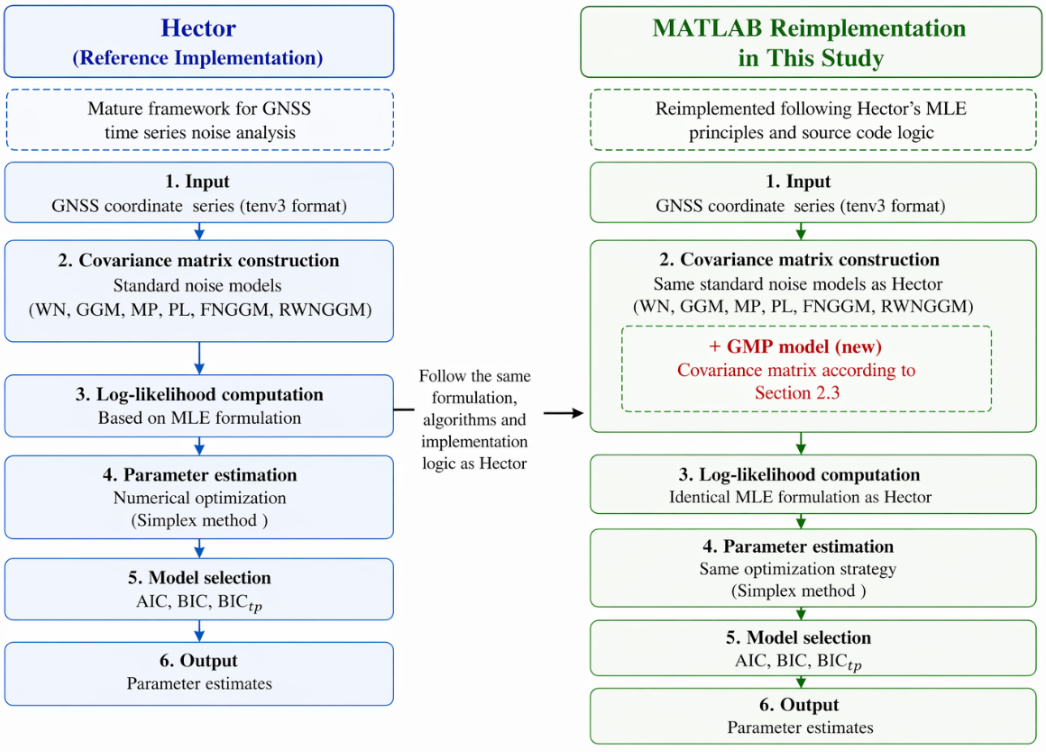
In this study, the Maximum Likelihood Estimation (MLE) procedure was implemented in MATLAB© R2023b following the same fundamental framework adopted in Hector, including the construction of the noise model covariance matrix, the computation of the log-likelihood function, and the numerical optimization strategy (as shown in Figure 1). Specifically, we reimplemented the relevant MLE components in MATLAB based on Hector’s established formulation and implementation logic. Extensive tests were carried out for the existing noise models, and the resulting parameter estimates and model selection statistics were found to be fully consistent with those obtained from Hector, confirming the reliability of our implementation. On this basis, the covariance matrix of the proposed GMP model was incorporated into the same mature MLE framework according to the theory developed in this section. Therefore, the only substantive extension with respect to the standard Hector-style implementation is the GMP-specific covariance representation, while the remaining likelihood evaluation and optimization procedures remain fully consistent with the well-tested Hector methodology.

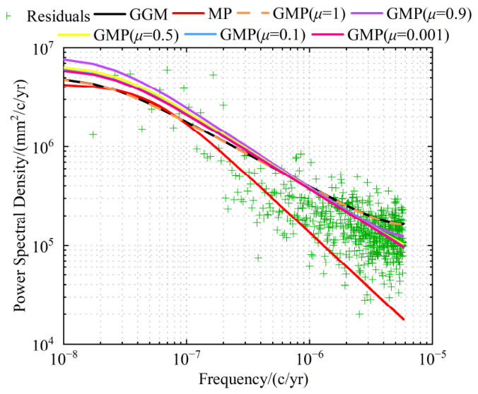
Next, we validate the ability of the parameter μ in the GMP to regulate the spectral shape by performing noise modeling on a real GNSS coordinate series. Figure 2 shows the PSD of the residuals of the east component GNSS coordinate series from the ANDA site in Andamooka, southern Australia, together with the PSDs of several noise models. The tested noise models include GGM, MP and GMP. The residuals were obtained by weighted least squares fitting, and the parameters of all noise models were estimated using MLE. For the GMP, μ was fixed at 1, 0.9, 0.5, 0.1 and 0.001, respectively.

As shown in Figure 2, the PSD curve of GMP (μ = 1) coincides exactly with that of the GGM. The PSD of GGM becomes flat at high frequencies, whereas the PSD of MP continues to decay in the high-frequency band. As μ in the GMP decreases gradually from 1 toward 0, the spectral shape of the GMP transitions from that of the GGM to that of the MP.

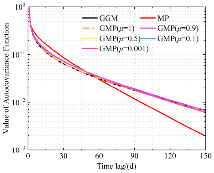
The corresponding Autocovariance Functions (ACFs) of these noise models are shown in Figure 3, which plots the first 150 ACF values. Consistent with Figure 2, the ACF curve of GMP (μ = 1) overlaps perfectly with that of the GGM. As μ decreases from 1 toward 0, the decay rate of the GMP ACF progressively shifts from the GGM-like decay toward the MP-like decay.

Accordingly, the PSD and ACF comparisons are used to characterize the colored stochastic structure remaining in the residual series after the deterministic functional components have been removed. They are not intended to uniquely attribute individual residual components to specific physical noise sources. The controlled simulation described in Section S4 of the Supporting Information File evaluates the extent to which deliberately unmodeled geophysical signals may affect stochastic noise-model identification.

It should be emphasized that μ is a stochastic shape parameter rather than a parameter associated with a unique physical noise source. Different physical processes may produce overlapping spectral characteristics and therefore a one-to-one correspondence between μ and a specific source of GNSS noise cannot generally be established. Instead, μ characterizes where the observed stochastic structure lies between the GGM-like and MP-like limiting behaviors.

2.4. Information Criteria and Akaike Weight

To compare the candidate noise models in a statistically rigorous manner, we employed three information criteria: the Akaike Information Criterion (AIC), the Bayesian Information Criterion (BIC) and the modified Bayesian Information Criterion (BIC_tp). These criteria are widely used for balancing model fit and model complexity in GNSS coordinate series noise analysis [22,32,33,34,35]. They are defined as

$$\mathrm{AIC}=-2\ln \left(L\right)+2k$$

(25)

$$\mathrm{BIC}=-2\ln (L)+k\ln (n)$$

(26)

$${\mathrm{BIC}}_{\mathrm{tp}}=-2\ln (L)+k\ln ({\displaystyle \frac{n}{2\pi }})$$

(27)

Equations (25)–(27) can be divided into two parts. The first term is the negative log-likelihood, where the likelihood function L is used to quantify how well a noise model fits the residuals. The second term is the penalty, where k is the number of parameters to be estimated in the noise model.

Although these criteria share the same general structure, they differ in the strength of the complexity penalty. AIC uses a constant penalty term 2k, whereas BIC applies the stronger penalty kln(n), which increases with the number of observations n. For long GNSS coordinate series, this often makes BIC more conservative than AIC when comparing models with different numbers of free parameters. The criterion BIC_tp is a modified form that retains the original factor 2$\pi$ appearing in the derivation of the Schwarz criterion and has also been adopted in geodetic stochastic model selection [22].

Because the absolute value of AIC has no direct probabilistic interpretation, Akaike weights were introduced to quantify the relative support for each candidate noise model under the AIC framework [26]. First, we compute the AIC increment:

$${\mathsf{\Delta }}_i={\mathrm{AIC}}_i-{\mathrm{AIC}}_{\min }$$

(28)

where ${\mathrm{AIC}}_i$ denotes the AIC value of the i-th candidate noise model and ${\mathrm{AIC}}_{\mathit{min}}$ denotes the AIC value of the optimal noise model. The relative likelihood of noise model i is proportional to exp(−Δ_i/2), defined as

$$p\left(y|M_i\right)\propto \exp \left(-{\displaystyle \frac{1}{2}}{\mathsf{\Delta }}_i\right)$$

(29)

Based on the above relationship, the Akaike weight $w_i$ can be defined to quantify the relative probability of different noise models [36]:

$$w_i={\displaystyle \frac{\exp \left(-\frac{1}{2}{\mathsf{\Delta }}_i\right)}{{\displaystyle \sum _{r=1}^R\exp \left(-\frac{1}{2}{\mathsf{\Delta }}_r\right)}}}$$

(30)

where R is the total number of candidate noise models. The Akaike weight $w_i$ can be interpreted as the relative support of model i within the candidate noise model set under the AIC framework, with ${\sum }_{i=1}^R{w}_i=1$.

It should be emphasized that noise model selection should not rely on a single information criterion. In this study, we adopt AIC, BIC and BIC_tp because they can be consistently incorporated into the maximum likelihood framework used for all candidate noise models. Therefore, the noise model selection results reported below should be interpreted as criterion-dependent statistical evidence rather than as proof of a universally optimal noise model. Greater confidence is placed on conclusions that remain qualitatively consistent across multiple criteria.

3. Determine the Robust Preferred Range of μ in GMP

This study aims to demonstrate that, compared with GGM and MP, GMP is a more general and advantageous noise model. As described in Section 2.3, a key issue in applying GMP is how to select the hyperparameter μ. From the perspective of information criterion, a direct comparison between GMP and GGM/MP is not entirely fair because the increased number of parameters leads to a larger complexity penalty. Moreover, μ may be intricately coupled with the remaining GMP noise parameters, λ and d, such that directly optimizing μ, λ and d via MLE could become trapped in local optima.

To determine a preferred range of hyperparameter μ, we adopted an enumeration strategy. Specifically, μ ∈ (0, 1] was fixed at 20 values with a step size of 0.05: 1, 0.95, 0.90, …., 0.05. In addition, to assess the behavior as μ → 0, we fixed μ at 5 smaller values: 0.01, 0.005, 0.001, 0.0001 and 0.00001. In total, 25 values of μ were tested.

To reduce the possibility that the experimental results might be biased by selecting data from a single geographical region, we selected 420 GNSS coordinate series from a total of 140 global GNSS sites distributed across different continents to comprehensively evaluate the preferred range of the hyperparameter μ in GMP. All the GNSS coordinate series data are obtained from the Nevada Geodetic Laboratory website (https://geodesy.unr.edu). Specifically, for each continent, 20 GNSS sites were selected, including 10 sites with the length of the GNSS coordinate series shorter than 10 years and 10 sites with the length of the GNSS coordinate series longer than or equal to 10 years (shown in

Table 1. The length of the 420 GNSS coordinate series from 140 global GNSS sites for testing the preferred range of hyperparameter μ in WN + GMP.

Geographical Location Area	Numbers of GNSS Coordinate Series
	Length < 10 Years	Length ≥ 10 Years
Asia	30	30
Europe	30	30
Africa	30	30
North America	30	30
South America	30	30
Oceania	30	30
Antarctica	30	30

), so as to examine the influence of series length on the preferred value of μ in GMP.

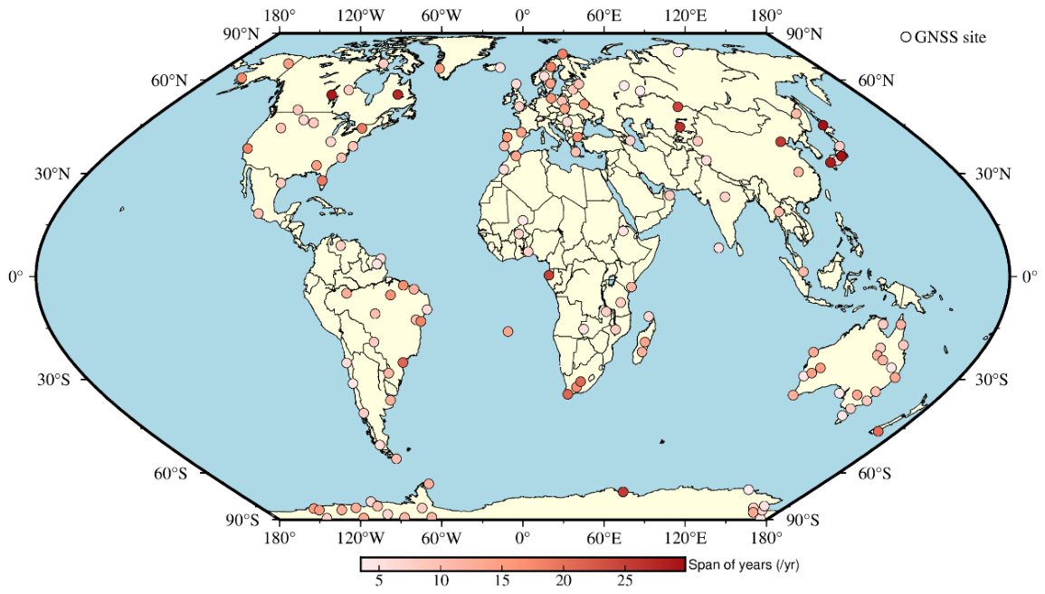
Figure 4 shows the geographical distribution of the 140 GNSS sites together with the lengths of GNSS coordinate series. As can be seen from the figure, the selected GNSS sites were chosen to account for a wide range of geographical settings. For example, we include 5 GNSS sites in Japan, 4 GNSS sites in the Andes mountains region of South America and 5 GNSS sites in the East African plateau to represent tectonically active regions. We select more than 10 GNSS sites from the European plains to represent relatively tectonically stable regions. We also include more than 20 GNSS sites from Antarctica and Greenland to represent ice covered regions. In addition, 7 GNSS sites from the Amazon region were selected to represent areas with pronounced periodic signals.

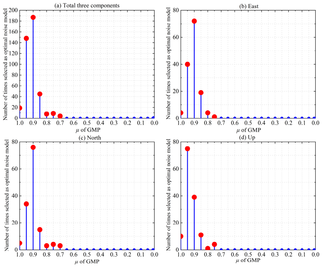
Figure 5 summarizes how often WN + GMP is selected as the optimal noise model when μ is fixed at different values. A clear and consistent pattern can be observed. For all three components, the preferred values of are concentrated mainly within the interval μ ∈ [0.7, 1], whereas values smaller than 0.7 are only rarely selected. Within this preferred interval, the highest selection frequencies occur at μ = 0.95 and μ = 0.9, with neighboring values such as μ = 0.85 and μ = 0.8 also occasionally selected, but much less frequently.

This result indicates that the optimal μ in WN + GMP should not be interpreted as a single universal value. Instead, the data support a robust preferred range close to the GGM end of the GMP family. The similarity of the distributions among the east, north and up components suggests that the preference for μ near 0.95~0.9 is not limited to one specific direction (shown in Figure 5b–d). Although the up component generally exhibits more complicated noise characteristics [5,18], its preferred μ values still remain concentrated in the same interval as those of the horizontal components.

The similar preferred μ interval among the three coordinate components does not imply that their stochastic characteristics are identical. The Up component generally exhibits larger noise amplitudes and stronger monument-related disturbances; however, these differences can also be absorbed by the noise amplitudes and the parameters λ and d. Therefore, the East, North and Up components may differ substantially in noise magnitude and correlation strength while still exhibiting a similar preferred range of μ.

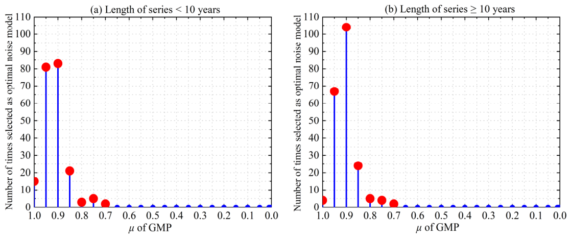
Figure 6 presents the statistics of the preferred μ values for GNSS coordinate series with different lengths. Despite the difference in time span, both show essentially the same overall tendency: the preferred values of μ are concentrated within the interval μ ∈ [0.7, 1] and the dominant peaks occur at μ = 0.95 and μ = 0.9. Values below 0.7 do not contribute to the optimal model counts in either group. These results suggest that the preferred range of μ is not controlled primarily by the length of GNSS coordinate series. However, as the length of the series increases, the preferred value of μ tends to decrease. This can be observed from the figure, where the peak in Figure 6b is shifted to the right along the horizontal axis compared with the peak in Figure 6a. Therefore, when analyzing the noise of long GNSS coordinate series, the preferred range of μ can be broadened appropriately.

Table 2. When the geographical location is different and the μ in GMP takes different values, WN + GMP is selected as the percentage of the optimal noise model.

Geographical Location Area	Percentage of Parameter μ in GMP to Be Selected as the Optimal Noise Model
	μ = 1	μ = 0.95	μ = 0.9	μ = 0.85	μ = 0.8	μ = 0.75	μ = 0.7
Asia	5%	35%	50%	6%	2%	2%	/
Europe	7%	48%	28%	12%	3%	2%	/
Africa	7%	27%	52%	7%	1%	5%	1%
North America	2%	42%	43%	11%	/	/	2%
South America	3%	33%	49%	10%	3%	2%	/
Oceania	/	33%	53%	10%	2%	2%	/
Antarctica	8%	28%	38%	18%	2%	3%	3%

shows the percentages with which WN + GMP is selected as the optimal model for different fixed values of μ in different geographical regions. Although some differences in the relative proportions of individual values can be observed among the seven regions, the preferred values remain predominantly concentrated within the interval μ ∈ [0.7, 1], particularly around μ = 0.95 and μ = 0.9.

To determine whether the apparent intercontinental differences in the preferred μ distributions are statistically significant, a Pearson chi-square test of homogeneity was performed using the original selection counts rather than the rounded percentages in Table 2. The resulting test statistic was ${\chi }^2=38.152$ with 36 degrees of freedom. Because several low-frequency categories contained small numbers of observations, resulting in expected frequencies below five in some cells, the statistical significance was additionally evaluated using a Monte-Carlo procedure with fixed marginal totals. The resulting Monte-Carlo p value was 0.368, consistent with the asymptotic chi-square p value of 0.372. Therefore, the null hypothesis that the preferred μ distributions are homogeneous across geographical regions cannot be rejected at the 5% significance level. The corresponding Cramér’s V was 0.123, indicating only a weak association between geographical region and the preferred value of μ.

These results indicate that the apparent differences among geographical regions are compatible with sampling variability at the present sample size. Although individual regions may show somewhat different relative preferences for neighboring values such as μ = 0.95 and μ = 0.9, no statistically significant intercontinental shift in the overall preferred μ distribution is detected. This supports the interpretation that μ is characterized by a robust preferred interval rather than by a geographically specific optimal value.

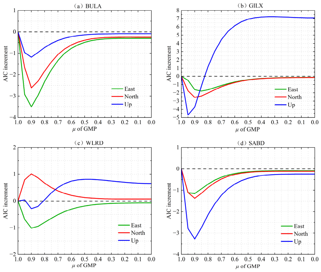
Figure 7 provides insight into the role of μ by showing the normalized AIC increments of WN + GMP as μ decreases for the east, north and up components of four representative GNSS sites (BULA, GILX, WLRD and SABD). Although the detailed shapes of the curves differ among sites and components, several common features can be identified. First, the AIC minima generally occur within the interval μ ∈ [0.7, 1]. Second, the exact location of the minimum is not identical for every series, which further supports the view that μ is better characterized by a stable preferred range than by a single exact value.

4. Noise Analysis of 846 GNSS Coordinate Series with Consideration of the GMP Model

4.1. GNSS Coordinate Series Data and Tested Noise Models

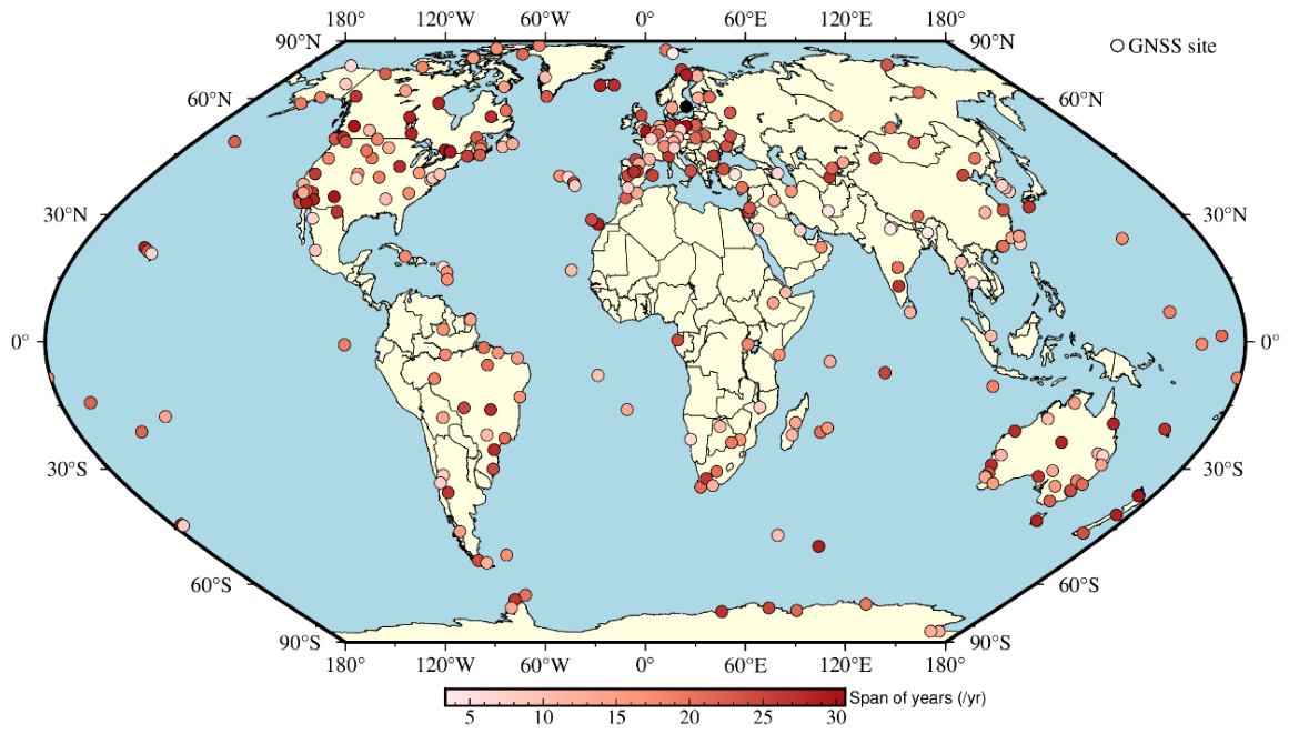
In this study, we selected 846 GNSS coordinate series from 282 global GNSS sites. The GNSS coordinate series data are obtained from the Nevada Geodetic Laboratory website (https://geodesy.unr.edu). The spatial distribution of the sites and the length information of the GNSS coordinate series at each site are shown in Figure 8.

As shown in Figure 8, the 282 selected GNSS sites are distributed over a broad global spatial extent. In selecting these sites, we attempted to avoid possible bias caused by using data from a single region or from a limited type of geophysical environment. The dataset therefore includes sites located in tectonically active regions, such as plate boundary zones and mountain belts, as well as sites in relatively stable continental interiors. It also includes both inland continental sites and island or coastal sites, so that GNSS coordinate series affected by different environmental and geodynamic conditions can be represented. In addition to spatial diversity, the selected GNSS coordinate series cover a wide range of lengths, from 3.5 to 30.7 years. This broad temporal coverage allows the applicability of the GMP model to be evaluated for both relatively short and long GNSS coordinate series.

Table 3. The length of the 846 GNSS coordinate series for 282 global GNSS sites.

Length of the Series	<5 Years	5~15 Years	15~25 Years	>25 Years
Number of the series	18	276	345	207
Percentage of series	2.1%	32.6%	40.8%	24.5%

summarizes the length statistics of the 846 GNSS coordinate series. Among them, series with lengths of 15~25 years constitute the largest group, with 345 series accounting for 40.8% of the total.

To evaluate the proposed GMP within a common parametric noise model framework, we considered a set of candidate noise models widely used in GNSS coordinate series analysis. The tested models include WN + GGM, WN + MP and WN + GMP, which are closely related in terms of spectral behavior and model construction, as well as several conventional noise models, namely WN + FN, WN + PL and WN + FN + RWN. This design enables the performance of GMP to be evaluated against its two endpoint-related models, GGM and MP, and against other commonly used parametric noise models under the same MLE and information criterion framework.

More flexible approaches have also been developed for GNSS coordinate series analysis, including fractal or multifractal noise descriptions, time-varying colored noise models and wavelet-based methods. These approaches involve different stochastic assumptions, model formulations and parameter estimation strategies and therefore cannot necessarily be compared directly with the models considered here using the same likelihood-based AIC, BIC and BIC_tp framework.

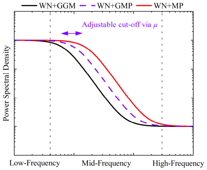
For a given GNSS coordinate series, the energy of its residuals at high and low frequencies is fixed. Therefore, in an ideal case, WN + GGM, WN + MP and WN + GMP provide comparable fits at both the low and high frequency ends and they share the same slope in the mid frequency band. The main difference lies in the location of the corner frequency from the low frequency to the mid frequency range, i.e., the length of the low-frequency plateau. As illustrated in Figure 9, suppose that for a GNSS time series, MLE yields a smaller corner frequency for WN + GGM and a larger corner frequency for WN + MP. As quantified in Section 2.3, the effective corner frequency of GMP is jointly controlled by μ and λ. The additional parameter therefore allows WN + GMP to shift the spectral transition between the GGM-like and MP-like regimes within the generalized model family.

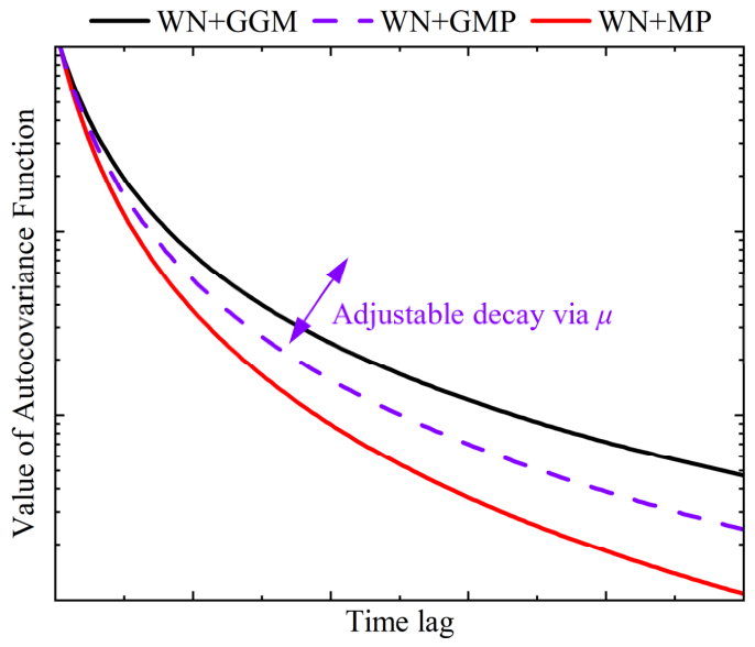
The relationships among the Autocovariance Functions (ACFs) corresponding to the above spectral behavior are illustrated in Figure 10. For the residuals of a given GNSS coordinate series, the total energy is fixed; thus, after normalization, the three noise models share the same starting value of the ACF. Because WN + GGM has a smaller corner frequency, its ACF decays more slowly, whereas the ACF of WN + MP decays more rapidly. As shown by the characteristic correlation time derived in Section 2.3, μ and λ jointly regulate the temporal correlation scale of GMP. Consequently, WN + GMP can produce an ACF decay behavior intermediate between those of the two endpoint models.

4.2. Noise Modeling Performance of GMP for GNSS Coordinate Series

We applied the candidate noise models introduced in Section 4.1 to perform noise modeling of the 846 GNSS coordinate series. It should be noted that following the results in Section 3, six representative members of the WN + GMP family were tested, namely WN + GMP (μ = 0.95), WN + GMP (μ = 0.9), WN + GMP (μ = 0.85), WN + GMP (μ = 0.8), WN + GMP (μ = 0.75) and WN + GMP (μ= 0.7). These values were selected from the preferred interval μ ∈ [0.7, 1] with a step size of 0.05. It should be emphasized that the purpose of the 846 series experiment is not to redetermine the preferred range of μ, which has already been systematically investigated using the 420 GNSS coordinate series in Section 3. Instead, the preferred interval identified in Section 3 is used here to construct a reduced WN + GMP candidate family for large-scale model validation. The AIC-based selection proportions of the individual fixed μ members for these 846 GNSS coordinate series are reported in

Table 4. Statistical proportions of the optimal noise models for 846 GNSS coordinate series under the AIC, BIC and BIC_tp criteria, based on noise modeling using WN + GGM, WN + MP, and the WN + GMP model family.

Information Criteria	Proportion of the Optimal Noise Model/(%)
	WN + GGM	WN + MP	WN + GMP Family Total	μ = 0.95	μ = 0.9	μ = 0.85	μ = 0.8	μ = 0.75	μ = 0.7
AIC	1.8	0.1	88.9	26.6	45.9	14.5	1.2	0.7	/
BIC	0.8	0.1	37.5	15.6	17.5	3.8	0.2	0.4	/
BICtp	0.9	0.1	50.1	18	25.2	5.9	0.5	0.5	/

.

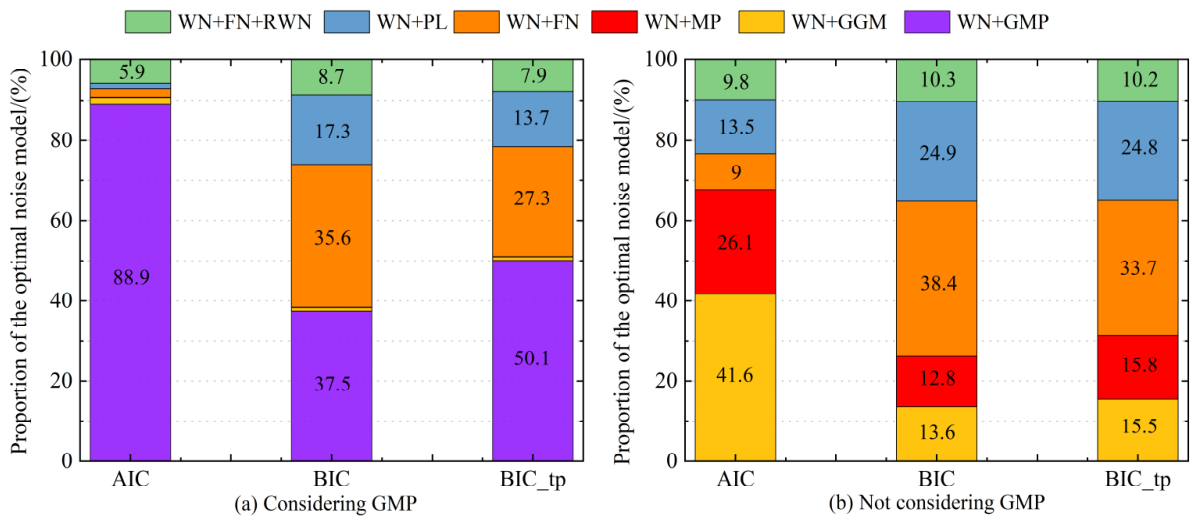
Results are shown in Figure 11 and Table 4. When the GMP family is included, the AIC results show a very strong preference for WN + GMP. The total proportion of the WN + GMP family reaches 88.9%, whereas WN + GGM and WN + MP are selected only 1.8% and 0.1% of the time, respectively. Within the GMP family, the dominant members are WN + GMP (μ = 0.9) and WN + GMP (μ = 0.95), accounting for 45.9% and 26.6%, respectively. By contrast, when the GMP family is excluded, the proportions of WN + GGM and WN + MP increase sharply to 41.6% and 26.1%, respectively. This shift indicates that many series previously assigned to the two endpoint models are more appropriately represented by intermediate members of the generalized family once these are made available. In other words, WN + GMP does not merely compete with WN + GGM and WN + MP; rather, it absorbs and refines them within a broader and more flexible stochastic framework.

Similar to the conclusion of [22], the BIC and BIC_tp results provide a stricter test because they impose a stronger penalty on model complexity. Under BIC, the total proportion of the WN + GMP family decreases to 37.5%, while WN + FN and WN + PL become more competitive, with proportions of 35.6% and 17.3%, respectively. Under BIC_tp, however, the total share of the WN + GMP family remains the largest at 50.1%, exceeding WN + FN (27.3%) and WN + PL (13.7%). These results show that the statistical preference for the WN + GMP family is sensitive to the choice of information criterion, but the overall conclusion remains robust: once a generalized family bridging GGM and MP is admitted, a large fraction of GNSS coordinate series are still better described by WN + GMP than by either endpoint model or by the more conventional alternatives.

Because the above noise model selection results are obtained from real GNSS coordinate series, residual geophysical signals not fully represented by the functional model may potentially affect stochastic model selection. To assess this possibility, we additionally conducted controlled simulations using prescribed WN + GMP stochastic backgrounds and three levels of deliberately unmodeled long-period geophysical signals. The simulations show that unmodeled signals can alter the proportions of the selected noise models and that the magnitude of this effect depends on the adopted information criterion. Importantly, substantial statistical support for the WN + GMP family is already present when no unmodeled geophysical signal is introduced, indicating that a preference for GMP can arise from the underlying stochastic structure itself rather than necessarily from compensation for residual geophysical signals. The detailed simulation design and results are provided in Section S4 of the Supporting Information File.

Table 5. Statistical proportions of the optimal noise models for 846 GNSS coordinate series under the AIC, BIC and BIC_tp criteria, when WN + GMP is modeled with different step sizes for μ within the preferred interval μ ∈ [0.7, 1].

Noise Model	Proportion of the Optimal Noise Model/(%)			Noise Model	Proportion of the Optimal Noise Model/(%)
	AIC	BIC	BICtp		AIC	BIC	BICtp
WN + GGM	1.8	0.8	0.9	WN + GGM	10.5	6.5	7
WN + MP	0.1	0.1	0.1	WN + MP	0.5	0.4	0.5
WN + GMP (μ = 0.95)	26.6	15.6	18	WN + GMP (μ = 0.9)	71.2	26.8	37.9
WN + GMP (μ = 0.9)	45.9	17.5	25.2
WN + GMP (μ = 0.85)	14.5	3.8	5.9	WN + GMP (μ = 0.8)	7.1	1.7	2.5
WN + GMP (μ = 0.8)	1.2	0.2	0.5
WN + GMP (μ = 0.75)	0.7	0.4	0.5	WN + GMP (μ = 0.7)	0.2	/	/
WN + GMP (μ = 0.7)	/	/	/
WN + FN	2	35.6	27.3	WN + FN	2	35.8	27.7
WN + PL	1.3	17.3	13.7	WN + PL	2.2	19.9	16.4
WN + FN + RWN	5.9	8.7	7.9	WN + FN + RWN	6.3	8.9	8

compares the optimal model proportions obtained when the parameter μ in the preferred interval is enumerated using two different step sizes. This comparison was introduced to address the concern that exhaustive enumeration of many μ values may increase computational cost. The results show that the main conclusion is insensitive to a moderate coarsening of the μ grid; the dominant solutions remain concentrated near μ = 0.9 and the overall preference for the GMP family is preserved across the AIC, BIC and BIC_tp.

More specifically, using a coarser step size mainly redistributes the winning proportions among neighboring μ values, rather than changing the qualitative model selection outcome. This is expected, because μ = 0.95, μ = 0.9 and μ = 0.85 already represent a narrow cluster of preferred solutions close to the GGM side of the GMP family. Therefore, reducing the density of the μ grid does not alter the physical or statistical interpretation of the results. This supports the use of a practical μ enumeration strategy in large-scale applications, especially when computational efficiency must be balanced against resolution in hyperparameter tuning. From a methodological point of view, Table 5 also strengthens the argument that μ should be interpreted as defining a robust preferred range rather than one uniquely meaningful fixed value.

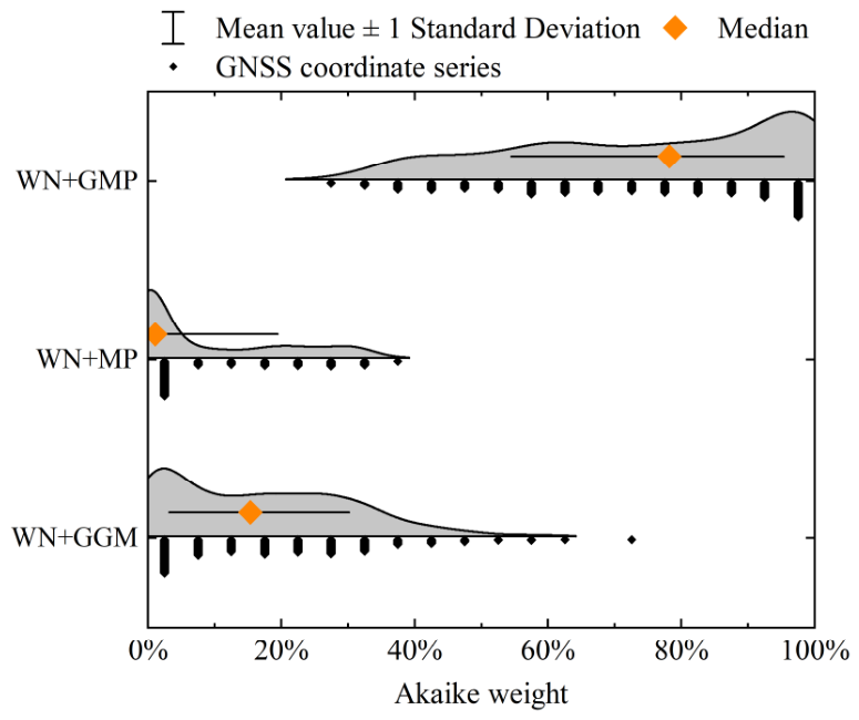
We also specifically investigated the performance differences among WN + GMP, WN + GGM and WN + MP in GNSS coordinate series noise modeling. Following the approach of [26], we computed the Akaike weights of the three noise models for each of the 846 GNSS coordinate series.

Intuitively, if the three noise models exhibit comparable modeling performance, their Akaike weights should cluster around 30%. Figure 12 presents the distribution statistics of Akaike weights for the WN + GMP family, WN + GGM and WN + MP. The results show that the Akaike weights of WN + GMP are concentrated between 40% and 100%, with a median of approximately 80%. In contrast, the Akaike weights of WN + MP are mainly distributed between 0% and 40%, with a median of around 2%, while those of WN + GGM are concentrated between 0% and 40%, with a median near 18%. These results indicate that, within the tested candidate model set and from an AIC-based perspective, WN + GMP receives substantially stronger statistical support than WN + GGM and WN + MP. This demonstrates the practical value of the proposed GMP model for GNSS coordinate series noise modeling.

4.3. Extraction of Velocity Signals from GNSS Coordinate Series Using GMP

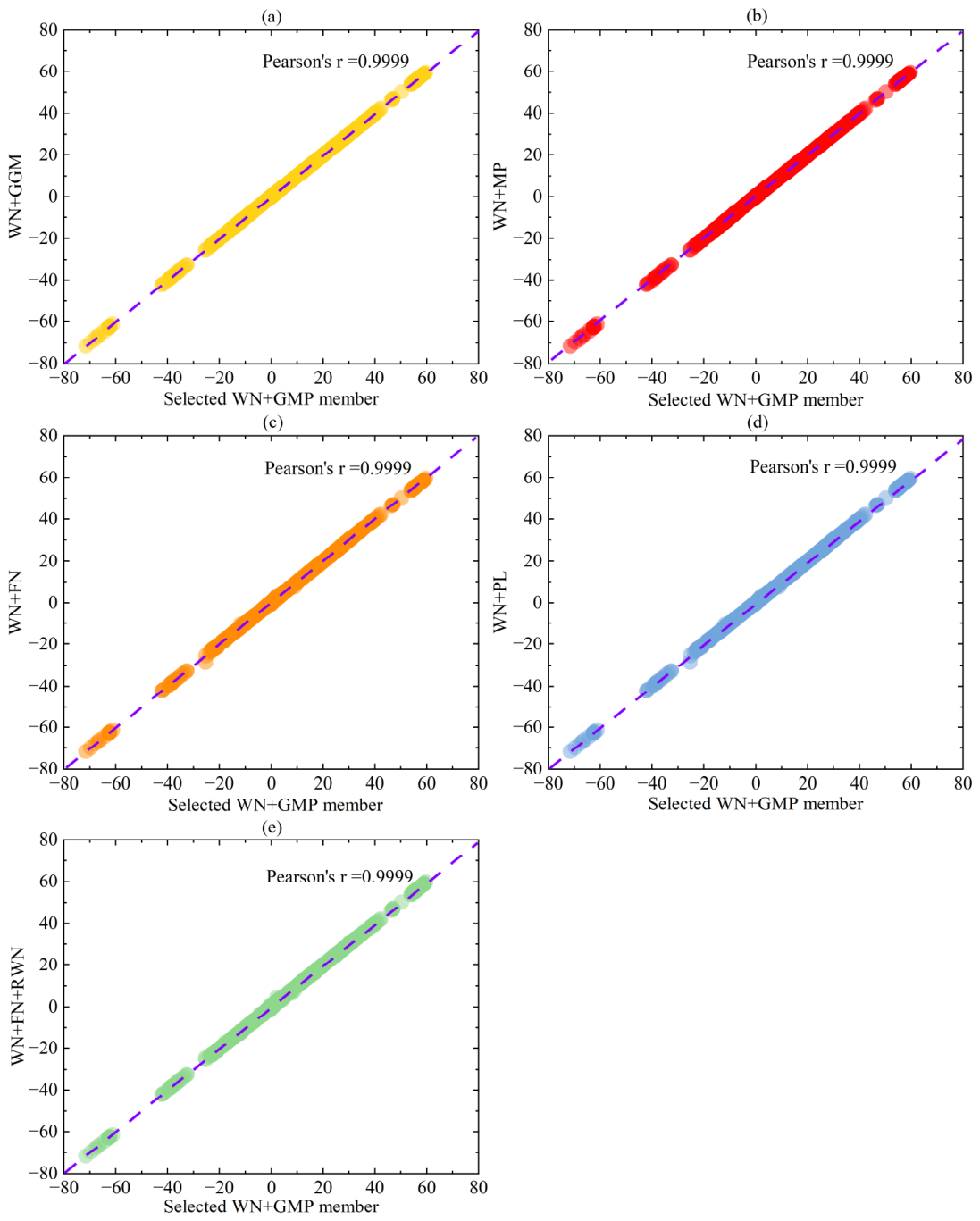
Figure 13 compares the GNSS site velocities estimated using different noise models with those obtained using the best-fitting WN + GMP member selected from the WN + GMP family for each coordinate series. For all tested models, the estimated velocities are almost perfectly aligned along the 1:1 diagonal, and the Pearson correlation coefficients are all close to 1. This result indicates that the extracted velocity signals themselves are highly stable with respect to the choice of noise model. Figure 13 shows that the practical role of the WN + GMP family is not to substantially alter the estimated velocities at most GNSS sites. Rather, its advantage lies in providing a more general and better supported stochastic description without sacrificing the stability of the extracted velocity signals.

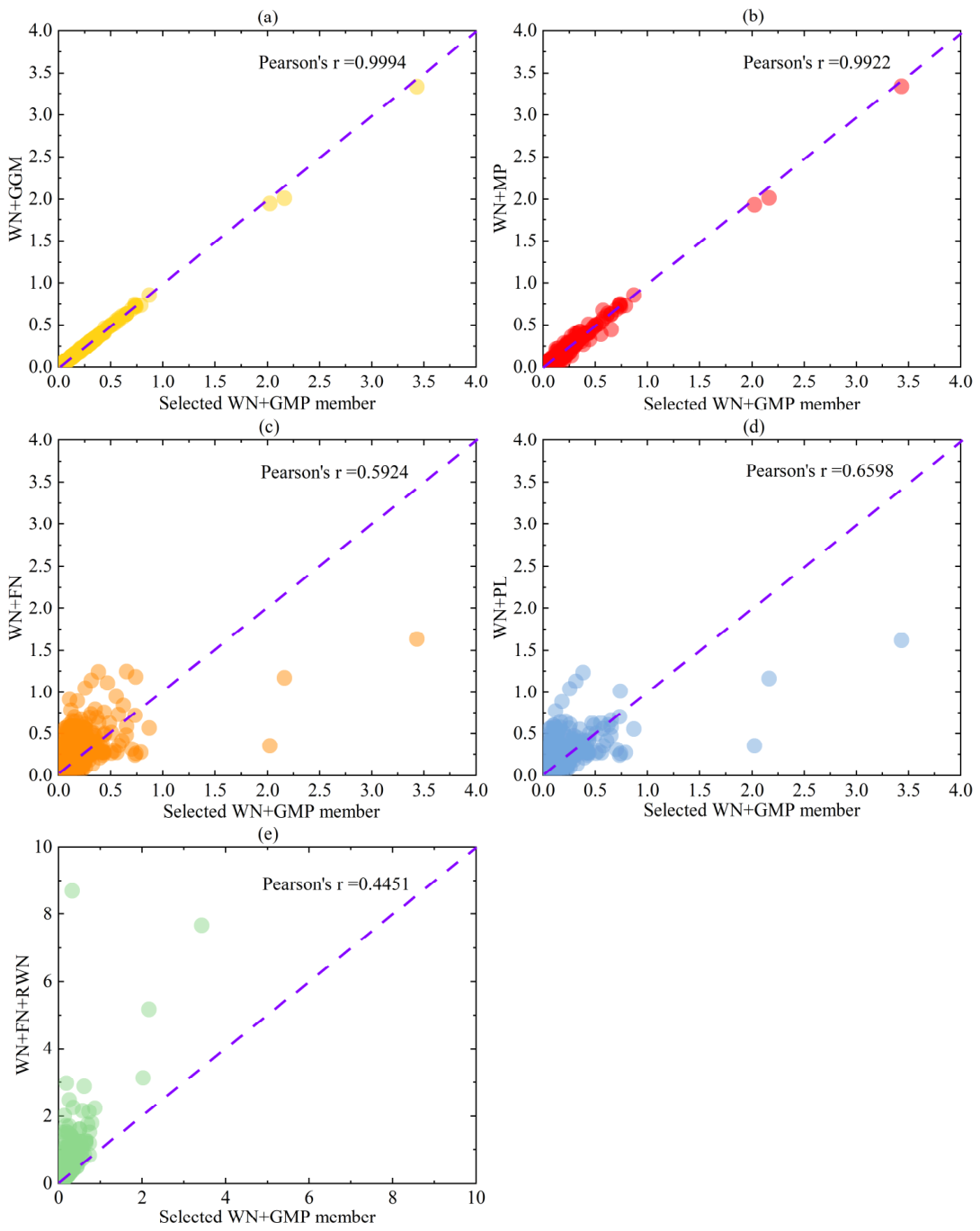
Figure 14 compares the velocity uncertainties estimated from different noise models with those obtained using WN + GMP. In contrast to the velocity estimates in Figure 13, the uncertainty estimates show more model-dependent differences. The uncertainties from WN + GGM are the closest to those from WN + GMP, with the scatter tightly concentrated near the 1:1 diagonal and a Pearson correlation coefficient of approximately 0.9994. The uncertainties from WN + MP also remain strongly correlated with those from WN + GMP, although the scatter is slightly larger. By comparison, the simpler conventional models, especially WN + FN + RWN, exhibit substantially broader dispersion and lower agreement with WN + GMP.

Although Pearson’s correlation coefficient characterizes the consistency of the uncertainty variations among different noise models, it does not directly quantify the magnitude or direction of their differences. Therefore, taking the uncertainty estimated using the best-fitting WN + GMP member for each coordinate series as the reference, we calculated the mean bias and RMSE for each alternative noise model. For noise model j, these quantities are defined as

$$\begin{array}{l}{\mathrm{Bias}}_j={\displaystyle \frac{1}{N}}{\displaystyle \sum _{i=1}^N\left({\sigma }_i^{\left(j\right)}-{\sigma }_i^{\left(GMP\right)}\right)}\\ {\mathrm{RMSE}}_j=\sqrt{{\displaystyle \frac{1}{N}}{\displaystyle \sum _{i=1}^N{\left({\sigma }_i^{\left(j\right)}-{\sigma }_i^{\left(GMP\right)}\right)}^2}}\end{array}$$

(31)

where N = 846, ${\sigma }_i^{\left(j\right)}$ is the velocity uncertainty, estimated using noise model j, and ${\sigma }_i^{\left(GMP\right)}$ is that obtained using the best-fitting WN + GMP member selected for the same GNSS coordinate series. Here, the mean bias represents the signed mean difference relative to the WN + GMP reference rather than bias with respect to an unknown true uncertainty.

The quantitative comparison in

Table 6. Quantitative comparison of GNSS site velocities estimated using different noise models relative to those obtained using the best-fitting WN + GMP member selected from the WN + GMP family.

Noise Model	Pearson’s r	Mean Bias (mm/yr)	RMSE (mm/yr)
WN + GGM	0.9999	0.0004	0.0121
WN + MP	0.9999	0.0005	0.0439
WN + FN	0.9999	−0.0085	0.1660
WN + PL	0.9999	−0.0074	0.1537
WN + FN + RWN	0.9999	−0.0111	0.1812

confirms the high stability of the estimated velocities with respect to the adopted noise model. All tested models exhibit Pearson correlation coefficients greater than 0.9999 relative to the selected WN + GMP member, while the absolute mean biases remain below approximately 0.012 mm/yr. WN + GGM shows the smallest deviation, with a mean bias of 0.0004 mm/yr and an RMSE of 0.0121 mm/yr.

In contrast to the velocity estimates, the velocity uncertainties exhibit more pronounced model dependence. As summarized in

Table 7. Quantitative comparison of GNSS site velocity uncertainties estimated using different noise models relative to those obtained using the best-fitting WN + GMP member selected from the WN + GMP family.

Noise Model	Pearson’s r	Mean Bias (mm/yr)	RMSE (mm/yr)
WN + GGM	0.9994	−0.0030	0.0093
WN + MP	0.9922	−0.0067	0.0247
WN + FN	0.5924	0.0710	0.1826
WN + PL	0.6598	0.0276	0.1473
WN + FN + RWN	0.4451	0.2550	0.8835

, WN + GGM and WN + MP remain close to the selected WN + GMP reference, with RMSE values of 0.0093 and 0.0247 mm/yr, respectively. By comparison, WN + FN, WN + PL and particularly WN + FN + RWN show substantially larger deviations. WN + FN + RWN yields the largest mean bias (0.2550 mm/yr) and RMSE (0.8835 mm/yr).

The comparisons in Figure 13 and Figure 14 should also be interpreted from the perspective of the generalized structure of the WN + GMP family. Since GGM and MP correspond to the endpoint or limiting cases of GMP, the purpose of introducing WN + GMP is not to force the estimated velocities or velocity uncertainties to be substantially different from those obtained using WN + GGM or WN + MP. On the contrary, when the stochastic characteristics of GNSS coordinate series are close to one of the endpoint models, WN + GMP is expected to produce results that are highly consistent with that endpoint model. The close agreement between WN + GMP and WN + GGM in the velocity and velocity uncertainty comparisons therefore reflects the inclusive nature of the GMP framework rather than a lack of practical value. More importantly, WN + GMP extends the model space beyond the two endpoints and allows intermediate stochastic structures between GGM and MP to be explicitly represented. Thus, the role of WN + GMP is not necessarily to generate markedly different geodetic outputs, but to provide a more general and flexible stochastic description while preserving the stability and physical plausibility of the extracted velocity signals.

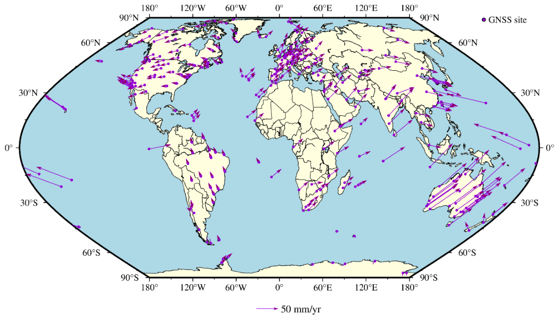
Figure 15 presents the horizontal velocity field estimated from WN + GMP for the 846 GNSS coordinate series. The resulting map displays the expected large-scale tectonic pattern, with coherent regional motions and no visually anomalous or unstable behavior caused by the use of the generalized stochastic model.

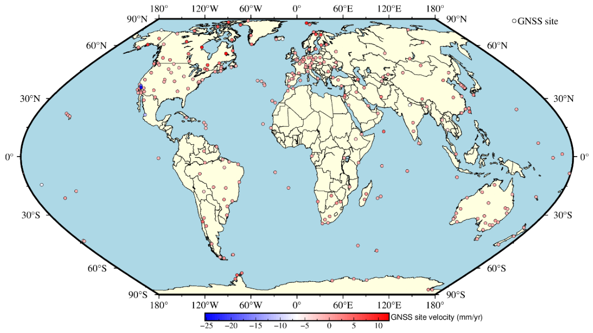
Figure 16 shows the vertical velocity field estimated from WN + GMP. Compared with the horizontal field, the vertical velocity field is spatially more heterogeneous, which is consistent with the generally stronger influence of local environmental loading, monument behavior and low-frequency noise on the up component of GNSS coordinate series.

5. Conclusions

This study reviews GGM and MP within a unified framework and, on this basis, proposes a generalized Matérn process (GMP) model family for GNSS coordinate series noise modeling. GMP introduces an additional fractional step-size parameter μ. When μ = 1, GMP is equivalent to GGM under the corresponding parameter mapping; as μ → 0, the spectrum of GMP approaches that of MP.

The preferred range of μ was investigated using 420 GNSS coordinate series from 140 global GNSS sites. The results show that the preferred μ values are mainly concentrated in the interval μ ∈ [0.7, 1]. This pattern is generally consistent across different directions, geographical regions and lengths of series. Therefore, μ should not be interpreted as a unique universal constant. Instead, it is more appropriate to regard μ as a hyperparameter that defines a robust preferred range close to the GGM side of the GMP family.

The noise model selection performance of the WN + GMP family is sensitive to the adopted information criterion, particularly to the stronger complexity penalty imposed by BIC. However, the overall model selection results also show that introducing the WN + GMP family improves the stochastic representation beyond using only the two endpoint models, WN + GGM and WN + MP. When the WN + GMP family is included, the selection proportions of WN + GGM and WN + MP decrease markedly, while intermediate WN + GMP members account for a substantial fraction of the optimal models. In addition, part of the optimal noise model selection proportions previously attributed to WN + FN, WN + PL and WN + FN + RWN are also replaced by members of the WN + GMP family. These results indicate that GMP is not merely a local extension of the two endpoint models but a competitive generalized model family within a broader GNSS noise modeling framework.

The velocity signal analysis confirms the practical role of the WN + GMP family in GNSS coordinate series analysis. For the core geodetic products, including velocity estimates and their uncertainties, the results obtained from the WN + GMP family are highly consistent with those from WN + GGM and WN + MP. This consistency should not be regarded as evidence that GMP is redundant. Instead, it reflects the desirable inclusive property of GMP as a generalized model; when the stochastic behavior of a coordinate series is close to the GGM or MP endpoint, the WN + GMP family can naturally reproduce results similar to those of the endpoint models. At the same time, the model selection results under AIC, BIC and BIC_tp show that the WN + GMP family provides stronger statistical support for a large fraction of GNSS coordinate series. Therefore, the advantage of WN + GMP lies in improving the stochastic noise representation while maintaining stable and physically consistent velocity signal estimates.

The GMP framework may also have potential for noise modeling of GNSS observations at other sampling rates, including hourly or higher-rate data, and it may provide a flexible background noise model for applications such as signal-to-noise assessment in GNSS seismology. However, the introduction of the additional hyperparameter μ increases model complexity and may complicate parameter estimation and model selection. In addition, the preferred μ range obtained from daily GNSS coordinate series may not be directly transferable to other sampling rates. Further studies are therefore needed to evaluate the applicability of GMP in these extended scenarios.

References

1. Bevis, M.; Brown, A. Trajectory models and reference frames for crustal motion geodesy. J. Geod. 2014, 88, 283–311. [Google Scholar] [CrossRef] [Scilit]
2. Gobron, K.; Rebischung, P.; Chanard, K.; Altamimi, Z. Anatomy of the spatiotemporally correlated noise in GNSS station position time series. J. Geod. 2024, 98, 34. [Google Scholar] [CrossRef] [Scilit]
3. Lv, H.; He, X.; Hu, S. Investigating surface loading effect on seasonal crustal deformation observed by GNSS in Hong Kong. Sci. Rep. 2025, 15, 2742. [Google Scholar] [CrossRef] [Scilit] [PubMed]
4. Dumitraschkewitz, P.; Mayer-Gürr, T. Handling temporal correlated noise in large-scale global GNSS processing. J. Geod. 2025, 99, 23. [Google Scholar] [CrossRef] [Scilit]
5. Klos, A.; Bos, M.S.; Bogusz, J. Detecting time-varying seasonal signal in GPS position time series with different noise levels. GPS Solut. 2018, 22, 21. [Google Scholar] [CrossRef] [Scilit]
6. He, X.; Montillet, J.-P.; Fernandes, R.; Melbourne, T.I.; Jiang, W.; Huang, Z. Sea Level Rise Estimation on the Pacific Coast from Southern California to Vancouver Island. Remote Sens. 2022, 14, 4339. [Google Scholar] [CrossRef] [Scilit]
7. Jiang, Z.; Zhang, Y.; Chang, M.; Tang, M.; Yang, X.; Yuan, Y. Weighted Laplacian smoothing constraints for terrestrial water storage changes considering GNSS station density: A case study in Pacific Northwest. GPS Solut. 2025, 29, 104. [Google Scholar] [CrossRef] [Scilit]
8. Okada, Y.; Nishimura, T. Investigation on short-term slow slip events in the northeast Japan subduction zones using decadal GNSS data. Earth Planets Space 2025, 77, 45. [Google Scholar] [CrossRef] [Scilit]
9. Xu, P.; Du, F.; Shu, Y.; Zhang, H.; Shi, Y. Regularized reconstruction of peak ground velocity and acceleration from very high-rate GNSS precise point positioning with applications to the 2013 Lushan Mw6.6 earthquake. J. Geod. 2021, 95, 17. [Google Scholar] [CrossRef] [Scilit]
10. Booker, D.; Clarke, P.J.; Lavallée, D.A. Secular changes in Earth’s shape and surface mass loading derived from combinations of reprocessed global GPS networks. J. Geod. 2014, 88, 839–855. [Google Scholar] [CrossRef] [Scilit]
11. Klos, A.; Dobslaw, H.; Dill, R.; Bogusz, J. Identifying the sensitivity of GPS to non-tidal loadings at various time resolutions: Examining vertical displacements from continental Eurasia. GPS Solut. 2021, 25, 89. [Google Scholar] [CrossRef] [Scilit]
12. Luo, X.; Wu, T.; Lu, L.; Chao, N.; Liu, Z.; Peng, Y. Using Geodetic Data to Monitor Hydrological Drought at Different Spatial Scales: A Case Study of Brazil and the Amazon Basin. Remote Sens. 2025, 17, 1670. [Google Scholar] [CrossRef] [Scilit]
13. Vidal, M.; Jarrin, P.; Rolland, L.; Nocquet, J.-M.; Vergnolle, M.; Sakic, P. Cost-efficient multi-GNSS station with real-time transmission for geodynamics applications. Remote Sens. 2024, 16, 991. [Google Scholar] [CrossRef] [Scilit]
14. Zhou, X.; Zhang, S.; Zhang, Q.; Liu, Q.; Ma, Z.; Wang, T.; Tian, J.; Li, X. Research of deformation and soil moisture in loess landslide simultaneous retrieved with ground-based GNSS. Remote Sens. 2022, 14, 5687. [Google Scholar] [CrossRef] [Scilit]
15. Wu, S.; Hu, X.; Zheng, W.; Berti, M.; Qiao, Z.; Shen, W. Threshold definition for monitoring Gapa Landslide under large variations in reservoir level using GNSS. Remote Sens. 2021, 13, 4977. [Google Scholar] [CrossRef] [Scilit]
16. Rebischung, P.; Gobron, K. Modeling random isotropic vector fields on the sphere: Theory and application to the noise in GNSS station position time series. J. Geod. 2024, 98, 79. [Google Scholar] [CrossRef] [Scilit]
17. Mao, A.L.; Harrison, C.G.A.; Dixon, T.H. Noise in GPS coordinate time series. J. Geophys. Res. Solid Earth 1999, 104, 2797–2816. [Google Scholar] [CrossRef] [Scilit]
18. Williams, S.D.P.; Bock, Y.; Fang, P.; Jamason, P.; Nikolaidis, R.M.; Prawirodirdjo, L.; Miller, M.; Johnson, D.J. Error analysis of continuous GPS position time series. J. Geophys. Res. Solid Earth 2004, 109, 19. [Google Scholar] [CrossRef] [Scilit]
19. Klos, A.; Bos, M.S.; Fernandes, R.M.; Bogusz, J. Noise-dependent adaption of the Wiener filter for the GPS position time series. Math. Geosci. 2019, 51, 53–73. [Google Scholar] [CrossRef] [Scilit]
20. Williams, S.D.P. The effect of coloured noise on the uncertainties of rates estimated from geodetic time series. J. Geod. 2003, 76, 483–494. [Google Scholar] [CrossRef] [Scilit]
21. Langbein, J. Noise in GPS displacement measurements from Southern California and Southern Nevada. J. Geophys. Res. Solid Earth 2008, 113, 12. [Google Scholar] [CrossRef] [Scilit]
22. He, X.; Bos, M.S.; Montillet, J.P.; Fernandes, R.M.S. Investigation of the noise properties at low frequencies in long GNSS time series. J. Geod. 2019, 93, 1271–1282. [Google Scholar] [CrossRef] [Scilit]
23. Langbein, J. Noise in two-color electronic distance meter measurements revisited. J. Geophys. Res. Solid Earth 2004, 109, 406. [Google Scholar] [CrossRef] [Scilit]
24. Bos, M.S.; Williams, S.D.P.; Araujo, I.B.; Bastos, L. The effect of temporal correlated noise on the sea level rate and acceleration uncertainty. Geophys. J. Int. 2014, 196, 1423–1430. [Google Scholar] [CrossRef] [Scilit]
25. Xu, C. An easy algorithm to generate colored noise sequences. Astron. J. 2019, 157, 127. [Google Scholar] [CrossRef] [Scilit]
26. Huan, Y.; Chang, G.; Huang, Y.; Feng, Y.; Zhu, Y.; Yang, S. Selection of noise models for GNSS coordinate time series based on model averaging algorithm. Meas. Sci. Technol. 2024, 35, 76305. [Google Scholar] [CrossRef] [Scilit]
27. Lilly, J.M.; Sykulski, A.M.; Early, J.J.; Olhede, S.C. Fractional Brownian motion, the Matérn process, and stochastic modeling of turbulent dispersion. Nonlinear Process. Geophys. 2017, 24, 481–514. [Google Scholar] [CrossRef] [Scilit]
28. Matérn, B. Spatial Variation; Springer Science & Business Media: Berlin/Heidelberg, Germany, 2013; Volume 36. [Google Scholar]
29. Xu, C. Fast and Robust Noise Background Modeling and Quasiperiodic Oscillation Detection for Astronomical Time Series. Astron. J. 2024, 168, 213. [Google Scholar] [CrossRef] [Scilit]
30. Kall, T.; Oja, T.; Kollo, K.; Liibusk, A. The noise properties and velocities from a time-series of Estonian permanent GNSS stations. Geosciences 2019, 9, 233. [Google Scholar] [CrossRef] [Scilit]
31. Li, Y.; Xu, C.; Yi, L.; Fang, R. A data-driven approach for denoising GNSS position time series. J. Geod. 2018, 92, 905–922. [Google Scholar] [CrossRef] [Scilit]
32. Santamaria-Gomez, A.; Bouin, M.-N.; Collilieux, X.; Woeppelmann, G. Correlated errors in GPS position time series: Implications for velocity estimates. J. Geophys. Res. Solid Earth 2011, 116, B01405. [Google Scholar] [CrossRef] [Scilit]
33. Li, W.; Wang, K.; Li, X. Spatial and temporal analysis of daily terrestrial water storage anomalies in China. Acta Geod. Geophys. 2024, 59, 427–440. [Google Scholar] [CrossRef] [Scilit]
34. Cucci, D.A.; Voirol, L.; Kermarrec, G.; Montillet, J.-P.; Guerrier, S. The Generalized Method of Wavelet Moments with eXogenous inputs: A fast approach for the analysis of GNSS position time series. J. Geod. 2023, 97, 14. [Google Scholar] [CrossRef] [Scilit] [PubMed]
35. He, X.; Bos, M.S.; Montillet, J.-P.; Fernandes, R.; Melbourne, T.; Jiang, W.; Li, W. Spatial variations of stochastic noise properties in GPS time series. Remote Sens. 2021, 13, 4534. [Google Scholar] [CrossRef] [Scilit]
36. Bozdogan, H. Model selection and Akaike’s Information Criterion (AIC): The general theory and its analytical extensions. Psychometrika 1987, 52, 345–370. [Google Scholar] [CrossRef] [Scilit]
Figure 1. Flowchart of the implementation principles of the MATLAB program used in this study.
Remotesensing 18 02932 g001
Figure 2. Power spectrum of the GNSS coordinate series residuals at ANDA, East component. The cross symbols denote the spectrum computed from the observations, and the colorful lines are the fitted multiple different noise models.
Remotesensing 18 02932 g002
Figure 3. Value of Autocovariance Function (for the first 150 time-lags). The Autocovariance Functions are obtained by fitting the residuals of GNSS coordinate series (ANDA, East component) using multiple noise models based on MLE.
Remotesensing 18 02932 g003
Figure 4. Geographical distribution map of 140 GNSS sites used for testing the preferred range of hyperparameter μ in WN + GMP.
Remotesensing 18 02932 g004
Figure 5. Number of times the WN + GMP model is selected as the optimal model when μ is fixed at different values in GMP when components of GNSS coordinate series are different: (a) are the results of all series in the total three direction components; (b) is the result in the East component; (c) is the result in the North component; (d) is the result in the Up component.
Remotesensing 18 02932 g005
Figure 6. Number of times the WN + GMP model is selected as the optimal model when μ is fixed at different values in GMP when lengths of GNSS coordinate series are different: (a) is the result of GNSS coordinate series with a length less than ten years; (b) is the result of GNSS coordinate series with a length greater than or equal to ten years.
Remotesensing 18 02932 g006
Figure 7. When using WN + GMP to model the GNSS coordinate series noise component of 4 GNSS sites, the variation in AIC of WN + GMP with μ. The black dashed line in the figure represents 0. (a) is the BULA site;(b) is the GILX site; (c) is the WLRD site; (d) is the SABD site.
Remotesensing 18 02932 g007
Figure 8. Geographical distribution map of 282 global GNSS sites.
Remotesensing 18 02932 g008
Figure 9. Schematic diagram of the relationship between the spectrum of WN + GGM, WN + MP and WN + GMP. The schematic diagram only illustrates this transition relationship, and the left and right positions do not represent fixed and unchanging parameter size patterns.
Remotesensing 18 02932 g009
Figure 10. Schematic diagram of the relationship between the autocovariance function of WN + GGM, WN + MP and WN + GMP. The schematic diagram only illustrates the trend of ACF attenuation speed and the left and right positions do not represent a fixed and unchanging parameter size pattern.
Remotesensing 18 02932 g010
Figure 11. Statistical proportions of the optimal noise models for 846 GNSS coordinate series under the AIC, BIC and BICtp criteria. (a) shows the proportions of the optimal noise models when the GMP model family is included; (b) shows the proportions of the optimal noise models when the GMP model family is not included.
Remotesensing 18 02932 g011
Figure 12. Statistical proportions of the Akaike weight distribution of the WN + GGM, WN + MP, and selected WN + GMP members in the experiment. The orange mark indicates the median position. The black solid line indicates the range of the mean value of the data ± one standard deviation. The black data points represent the distribution of GNSS coordinate series.
Remotesensing 18 02932 g012
Figure 13. Consistency analysis of GNSS site velocities estimated using different noise models relative to those obtained using the best-fitting WN + GMP member selected from the WN + GMP family for 846 GNSS coordinate series. (a) Comparison between WN+GGM and the selected WN+GMP member; (b) comparison between WN+MP and the selected WN+GMP member; (c) comparison between WN+FN and the selected WN+GMP member; (d) comparison between WN+PL and the selected WN+GMP member; (e) comparison between WN+FN+RWN and the selected WN+GMP member.
Remotesensing 18 02932 g013
Figure 14. Consistency analysis of GNSS site velocity uncertainties estimated using different noise models relative to those obtained using the best-fitting WN + GMP member selected from the WN + GMP family for 846 GNSS coordinate series. (a) Comparison between WN+GGM and the selected WN+GMP member; (b) comparison between WN+MP and the selected WN+GMP member; (c) comparison between WN+FN and the selected WN+GMP member; (d) comparison between WN+PL and the selected WN+GMP member; (e) comparison between WN+FN+RWN and the selected WN+GMP member.
Remotesensing 18 02932 g014
Figure 15. Horizontal velocity field estimated from noise modeling of the 846 GNSS coordinate series using WN + GMP.
Remotesensing 18 02932 g015
Figure 16. Vertical velocity field estimated from noise modeling of the 846 GNSS coordinate series using WN + GMP.
Remotesensing 18 02932 g016