Article

NWCSAF High Resolution Winds (NWCSAF GEO-I HRW) Stereo AMVs over the Atlantic Ocean
1
Agencia Estatal de Meteorología (AEMET), 28040 Madrid, Spain
2
Carr Astronautics Corporation, Greenbelt, MD 20770, USA
3
Earth System Science Interdisciplinary Center, University of Maryland, College Park, MD 20742, USA
4
Atmospheric and Planetary Sciences Department, Hampton University, Hampton, VA 23669, USA
5
NASA/Goddard Space Flight Center, Greenbelt, MD 20771, USA
*
Author to whom correspondence should be addressed.
Remote Sens. 2026, 18(17), 2940; https://doi.org/10.3390/rs18172940
Submission received: 15 May 2026 / Revised: 10 August 2026 / Accepted: 18 August 2026 / Published: 1 September 2026
(This article belongs to the Special Issue New Insights from Wind Remote Sensing)

Highlights

What are the main findings?
  • The “stereo height assignment method” developed previously for NASA and NOAA has been included in the NWCSAF High Resolution Winds (NWCSAF GEO-I HRW) AMV product for geostationary AMVs in the region jointly observed by MTG-I1 and GOES-East over the Atlantic Ocean.
  • A comparison of stereo AMVs with non-stereo AMVs has also taken place, based on ECMWF ERA5 reanalysis winds and EarthCARE ATLID Mie Attenuated Backscatter (MAB) LiDAR curtains, with many examples where the stereo method improves height assignments, especially at high levels (>6 km).
What are the implications of the main findings?
  • The stereo method can better represent the state of the atmosphere and provide a tool for validating and improving non-stereo height assignments.
  • The updated High Resolution Winds algorithm will be released to NWCSAF users in 2027 and will support additional studies to improve the existing non-stereo height assignment methods.

Abstract

The “stereo height assignment method” developed for NASA and NOAA for GOES-R ABI Atmospheric Motion Vectors (AMVs), a purely geometric method using the parallax observed from different satellites, has been included in the NWCSAF AMV product (NWCSAF GEO-I HRW, High Resolution Winds) as an additional height assignment option for AMVs in the region jointly observed by MTG-I and GOES-East over the Atlantic Ocean. Stereo and the alternative non-stereo height assignment (“Cross Correlation Contribution (CCC)”) are compared with ECMWF ERA5 reanalysis winds and EarthCARE ATLID Mie Attenuated Backscatter (MAB) curtains. For low-level clouds, both methods generally conform well with apparent cloud tops in MAB curtains. For higher clouds, more differences are seen between stereo and non-stereo heights. Compared with ERA5 winds, stereo shows the most improvement above 6 km. However, the stereo method produces 70–90% less AMVs since additional high-quality matches are needed from both FCI and ABI imagery. An updated HRW will be released to NWCSAF users in 2027 as version “NWCSAF GEO-I v2027.” The combined provision of both stereo and non-stereo CCC height assignment methods will enable further studies (already planned) of the AMV best-fit level for different satellite channels and cloud types, heights and depths.

1. Introduction

The Satellite Application Facility on Support to Nowcasting and Very Short Range Forecasting (NWCSAF) is a consortium inside the European Organisation for the Exploitation of Meteorological Satellites (EUMETSAT) Satellite Application Facility (SAF) network consisting of five European National Meteorological Services: AEMET/Agencia Estatal de Meteorología of Spain, Météo-France, GeoSphere Austria, SMHI/Sveriges Meteorologiska och Hydrologiska Institut of Sweden, and ANM/Administrația Națională de Meteorologie of Romania. The work of the Consortium started in 1997.
The main objective and requirement of the NWCSAF is to produce stand-alone software packages, which calculate in near real-time meteorological products from geostationary and polar satellite data. These software packages are installed locally at the user’s site to enhance nowcasting and very short-range forecasting (i.e., weather forecasting up to 12 h). As stand-alone software packages, they contain all the elements for the calculation of the products without the need for any other elements, beyond the corresponding input data. The NWCSAF also supports its users in the generation and application of the products.
Among the NWCSAF meteorological products, there is a product calculating Atmospheric Motion Vectors (AMVs) and trajectories through the displacement of cloud and humidity features in successive satellite images: High Resolution Winds (HRW), present in both the geostationary software package NWCSAF GEO-I (since its first version in 2004) and the polar software package NWCSAF PPS (since 2021).
An Atmospheric Motion Vector (AMV) is the horizontal displacement of the Earth position of a tracer or N × N pixel pattern seen in a satellite image pair. A trajectory is the path defined by the displacement of the same tracer throughout several satellite images. The tracer is defined through a specific cloud feature in visible, infrared or water vapor images (and so-called “cloudy AMV”) or through a specific humidity feature in cloudless areas in water vapor images (and so-called “clear air AMV”).
AMVs are associated with the horizontal wind in the atmosphere and are useful in nowcasting applications, used in synergy with other data available to the forecaster. For example, they are used in the watch and warning of dangerous wind situations; in the monitoring of the general atmospheric flow, of low-level convergence (when and where cumulus clouds start to develop), and of divergence at the top of developed systems; and in other cases of small-scale circulation or wind singularities. They can also be assimilated in Numerical Weather Prediction (NWP) models (together with other data) or used as input in analysis, nowcasting and very short-range forecasting applications. For example, HRW output is currently being assimilated by NWP models by the National Meteorological Services of Austria, Hungary and the United Kingdom and is being tested by those of Finland, Norway and Australia (in the last case with Himawari).
A detailed description of the product and comparison with other AMV products worldwide up to 2019 can be found in García-Pereda et al., 2019 [1]. Further updates, including the extension to the new MTG-I satellite series over Europe and Africa in the geostationary version and up to six different polar satellite series in the polar version, can be found in the latest Algorithm Theoretical Basis Documents (ATBDs) and Validation Reports (VRs) [2,3,4,5]. Relevant advantages of this product are that it calculates AMVs in all corners of the world using the same algorithm for both geostationary and polar satellites (which can be important for assimilation in global NWP models, including reanalysis, and for climatic studies), and that the validation results obtained for all satellite series are very similar.
The main source of error for the HRW AMV product has always been (as in general for other AMV products throughout the world [6]) the height assignment process (the vertical location of the AMVs and trajectories, as their height or pressure level in the atmosphere). Two different methods of height assignment have been used up to now in HRW: the “brightness temperature interpolation method” (default option in the initial versions of the algorithm) and the “Cross Correlation Contribution (CCC) method” (as defined in Borde & Oyama, 2008 [7], and which became the default option in the HRW algorithm since the year 2011). The full details of these height assignment methods are available in García-Pereda, 2025a [2]. These methods imply, however, a dependence on the algorithms and outputs of several NWCSAF Cloud products (“CT/Cloud Type”, “CTTH/Cloud Top Temperature and Height” and “CMIC/Cloud Microphysics”). They also depend on up to 16 NWP forecast variables directly inside the HRW algorithm or inside the Cloud algorithms.
In contrast, the purely geometric “stereo height assignment method” has been identified as an alternative at least since the Second International Winds Workshop in 1993 [8]. The method simply considers the parallax of a tracer/AMV observed by two different satellites. The displacement (difference in the apparent position) of the tracer/AMV over the Earth’s surface when viewed by these two satellites is directly related to the height of the tracer/AMV over the Earth’s surface (Figure 1). However, several limitations were identified in the method since it was first proposed, the main ones being that the “stereo height assignment method” can only be used for locations in which tracers/AMVs are observed at the same time by two different satellites with relatively large angle differences, and that asynchronous observations by the two different satellites need to be corrected.
Only with the newer generation of geostationary satellites (Himawari-8/9, GOES-R, MTG-I), with their better spatial resolution and high-accuracy geo-registration, has there been a push for the inclusion of the “stereo height assignment method” in the operational AMV algorithms, as shown in the Sixteenth International Winds Workshop by Carr et al., 2023a [9].
Since 2018, NASA-NOAA collaborations have been developing stereo methods to define AMV heights, enabled by the excellent geometric accuracy of the latest-generation operational satellites. This allows for the direct geometric determination of the AMV height in the atmospheric column, independent of NWP, with the expectation that geometric height assignments are more reliable and accurate than those inferred from other currently existing methods. The ability to time-tag pixels and include timing differences in modeling the trajectories of tracers now allows for non-simultaneous scenes from different satellites to be used [10].
The stereo wind method has been developed for several different cases, including pairs of geostationary satellites [10], a geostationary and a polar-orbiting satellite [11,12], and multiple polar-orbiting satellites [13]. The description of the stereo implementation for HRW presented here draws on work originally supported by NASA and later by NOAA using the ABI radiometer [10]. Research implementations of stereo AMVs exist at NASA and NOAA, with the latter being prepared for a transition to an operational product supporting pairs of GOES-R and Himawari-8/9 satellites. Future operational extensions at NOAA may include ABI-VIIRS stereo AMVs. The NASA research code has been used for several studies, including ones involving volcanoes [14,15,16,17], wildfires [18,19], von Karman vortices [20], and the diurnal cycle of the boundary layer [21]. Recent work by others includes a study of cloud-top heights with the Chinese FY-4A and -4B satellites [22], an investigation of cloud entrainment in the boundary layer from stereo observations constrained by the continuity equation for mass flow [23], and a theoretical study of stereo cloud-top height retrieval accuracy versus modeled cloud fields [24].
Because of this body of prior work, a “Visiting Scientist Activity (VSA)” was defined between the NWCSAF, the University of Maryland, and the Carr Astronautics Corporation (with additional contributions by NASA) to include in HRW v2025 all code extensions needed to implement the “stereo height assignment method” for the AMVs located in the region covered by both MTG-I and GOES-East. This paper describes this implementation in HRW and compares the stereo height assignments and those of the CCC method to assess which better represents the true atmospheric motion (wind).
The “stereo height assignment method” implemented here will be available for NWCSAF users inside the following software package version (NWCSAF GEO-I v2027), to be released in early 2027.

2. Materials and Methods

2.1. Methodological Workflow

The methodological workflow for this work involved integrating the GEO–GEO stereo height assignment into the NWCSAF GEO-I HRW v2025 (vMTG-I day-1) algorithm, validating the resulting stereo-derived AMV heights and pressures and assessing their operational limits and performance relative to existing height assignment techniques. All development was conducted in close coordination with the NWCSAF Project Team and aligned with complementary NASA-supported validation activities. The implementation supports multiple stereo configurations: three- to six-image combinations of MTG-I/FCI FDHSI and GOES-East/ABI full-disk imagery.
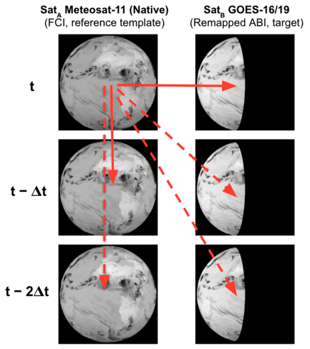
The GEO–GEO stereo wind methodology relies on two to three temporally separated repetitions from the reference satellite (SatA, and one to three repetitions from the secondary satellite (SatB), with the constraint that all repetitions within each satellite originate from the same scene type and channel/band pairing. In this study, MTG-I serves as SatA and provides the native fixed grid and reference template to serve as the tracer, while GOES-East serves as SatB and is fully remapped to the MTG-I grid. This reprojection step yields a region on the western edge of the MTG-I disk where corresponding GOES-East pixels exist within the GOES-East horizon. Figure 2 illustrates the temporal pairing strategy used for the stereo retrievals, showing the use of MTG-I images at times t, t–Δt, and t–2Δt in combination with one or more temporally aligned GOES-East images. The overall approach follows the framework described in Carr et al., 2020 [10], adapted here for the MTG-I and GOES-East pairing. Up to seven bands can be used by HRW with the FCI radiometer for AMV calculation (VIS06, VIS08, IR038, WV063, WV073, IR105, IR123), which are paired, respectively, in the ABI radiometer with the equivalent bands 2, 3, 7, 8, 10, 13, 15 in the same part of the spectrum. At least one pairing with SatB is required to observe the parallax of the tracer and derive the height. Additional pairings may be considered, as will be discussed later.

2.2. Integration of the Stereo Functionality into HRW Processing

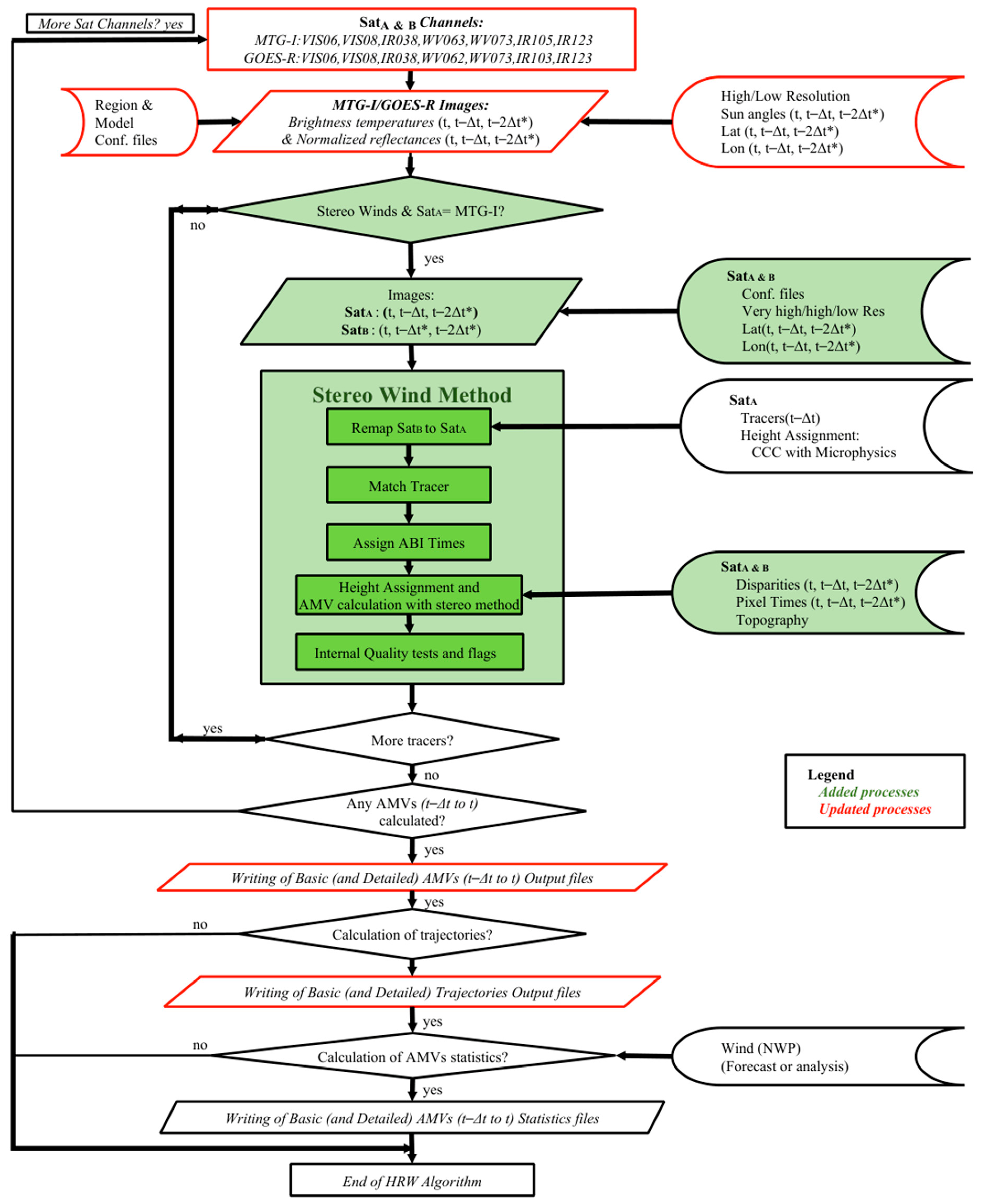
Figure 3 illustrates how the stereo height assignment functionality is integrated into the HRW processing chain. This functionality is included as an additional capability within the existing HRW processing (with more details in Friberg et al., 2025 [25]). So, if it is skipped, the process remains exactly equivalent to the previous non-stereo one. Due to this, once each tracer is defined, tracked and height-assigned using the original process (using “Cross Correlation Contribution height assignment method” in the default configuration), the stereo height is calculated. For this, after remapping all ABI scenes to the FCI fixed grid, the stereo module performs image registration to match and assign a time for each tracer across all SatA and SatB images (using the same cross-correlation method used for the non-stereo AMVs). The stereo module then computes the 3-D AMV solution, deriving stereo heights, pressures, and displacement vectors. Once the stereo processing is complete, the processing returns to the original HRW workflow, where the original quality control screening takes place, the AMVs are compiled across all processed channels, trajectory information is calculated, and both basic and detailed output files (if so configured) are written. The diagram highlights the modular insertion of the stereo method within the existing HRW architecture, ensuring compatibility with the operational HRW processing steps downstream.

2.3. Remapping of GOES-R/ABI Images into MTG-I/FCI Geometry

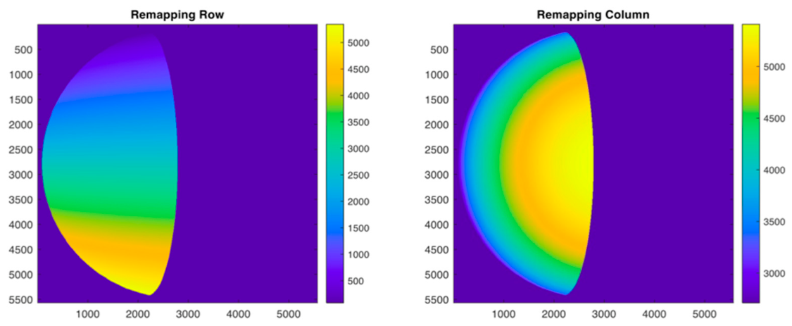
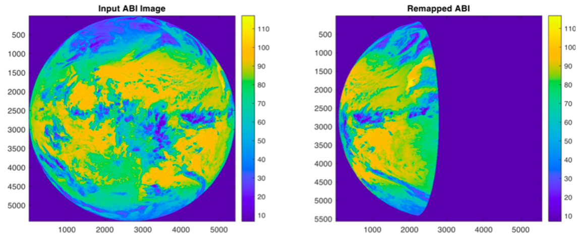
To enable the tracer matching across all images and so the stereo height retrievals, the GOES-East imagery used as the secondary satellite input is reprojected into the native MTG-I viewing geometry using Look-Up Tables (LUTs) (Figure 4). LUTs are calculated once and saved in auxiliary NetCDF files. Remapping LUTs are applied to the ABI images to remap them into the FCI fixed grid (Figure 5). The process looks up a floating-point row and column address at each FCI pixel location and interpolates the value for that location from a neighborhood of the site addressed in the ABI image. Bilinear interpolation is used. The corresponding reprojection errors have not been specifically quantified within the timeframe of this study.

2.4. MTG-I/FCI and GOES-R/ABI Pixel Times

The handling of FCI pixel acquisition times was revised to use channel-specific data obtained from the FCI satellite images, replacing the earlier approximation in HRW that applied the same values across all channels. This per-channel implementation accounts for small but meaningful timing differences inherent to FCI’s scanning strategy.
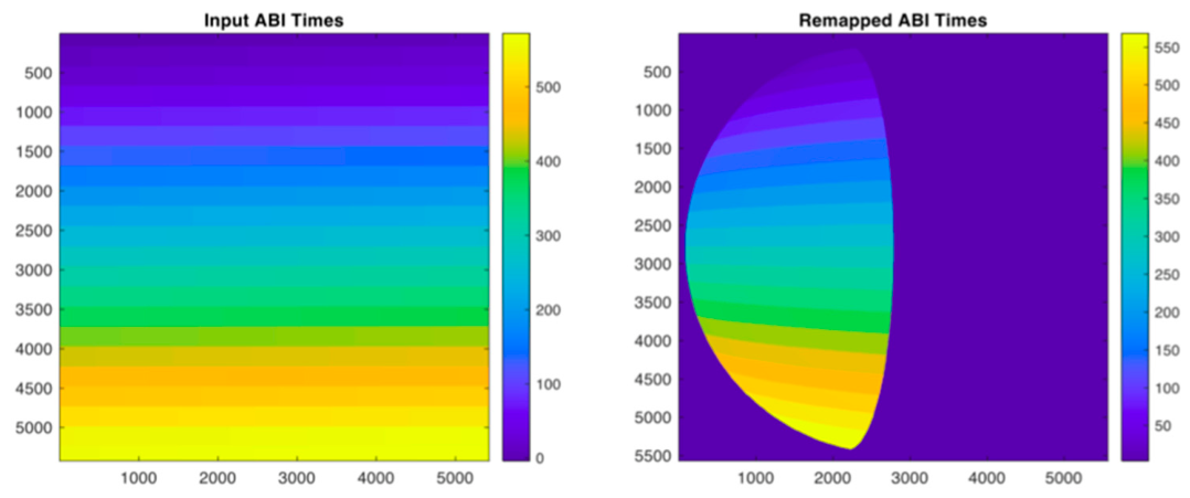
Specifically defined LUT-based pixel acquisition times are used for the ABI images, valid for Mode 6 full-disk scanning, which provide a more accurate representation of ABI pixel acquisition times than the scan rate and speed model previously used by the HRW algorithm (ABI satellite files do not provide per-pixel acquisition time information). This LUT-based pixel time model for ABI pixels is shown in Figure 6 below, based on increments in seconds with respect to the “product time” (encoded after “s” for “start” in the satellite file name). More details about how these LUTs were defined can be found at Carr et al., 2020 [10].
Both changes in pixel acquisition time for MTG-I and GOES-R also imply a slight improvement in the AMVs for MTG-I and GOES-R satellites when the stereo process is not used and are made available to users in the NWCSAF GEO-I HRW v2025.2 patch.

2.5. Stereo Parallax and Height

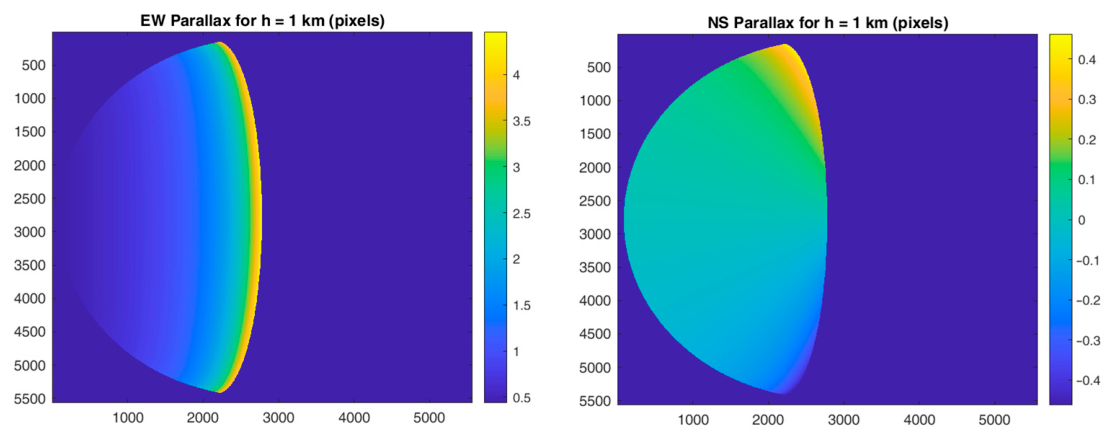
An initial guess for the stereo wind vectors and heights was made considering the non-stereo AMV obtained previously with the original HRW procedure. With this, other than initializing the stereo search window for efficiency, the NWP does not enter into the stereo wind retrieval. Additional LUTs are provided to translate a kilometer of altitude into a parallax (Figure 7).
After the tracer matching between images from the two satellites, parallax measurements are converted into geometric heights using the satellite ephemerides and full viewing-geometry information for both platforms, after which equivalent pressure levels are obtained through standard HRW thermodynamic conversion routines. The resulting quantities, “AMV stereo height” and “AMV stereo pressure,” are integrated directly into the HRW output structure alongside existing non-stereo height assignments. All newly developed modules were validated for numerical consistency, error-handling robustness, and full compatibility with the operational HRW processing chain.

2.6. Stereo Wind Retrieval

The stereo wind retrieval itself is formulated as an optimization problem that uses the apparent positions of a tracer observed multiple times by SatA and SatB. Using a reference scene from SatA at time t, and additional scenes from both SatA and SatB at t and adjacent t as shown in Figure 2, the algorithm solves for the height and horizontal motion for each tracer by minimizing weighted residuals between modeled and observed displacements. Two models (configurable) are supported: a three-parameter (order-3) version, which calculates the height and the components of the horizontal displacement of the tracer (h, u, v), and a five-parameter (order-5) version which additionally calculates a horizontal relocation of the tracer related to potential image-navigation errors (h, u, v, Δx, Δy).
The five-parameter version is preferred because it provides a richer representation of the feature and its motion, and because its need to process more images from both satellites increases the trust in the tracking process. It also absorbs systematic navigation biases and yields more noise-like residuals, which are essential for quality control.
The problem is solved iteratively using linearized updates, with convergence assessed via position and velocity tolerances. Overdetermination, using more scenes than the minimum required, improves robustness but must be balanced against the assumption that tracers translate without evolving.
Appendix A provides a full mathematical description of how this works.

2.7. Control Check and Output-Filtering Procedure

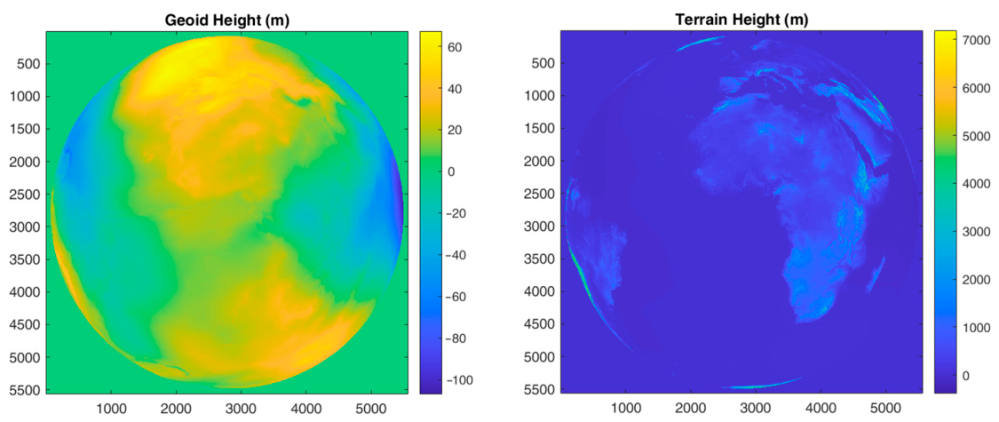
The final stage of the stereo workflow applies a consolidated control check and output-filtering procedure to ensure that the retrieved winds, heights, and parallax values are geometrically consistent and scientifically robust. Unlike the traditional CCC method used in the non-stereo HRW chain, which emphasizes the most visually striking feature within a cloud pattern, the stereo implementation defines the height of patterns at the centers of the tracked cloud features explicitly. This enables direct comparison of disparities between the two satellites in terms of paired latitude–longitude displacements. These disparities feed into the stereo height solution, which now incorporates geoid-referenced height information for computing pressure more accurately (Figure 8).
To capture the quality of the stereo fit, the system produces residual metrics derived from the difference between measured and modeled disparities. The residual sum of squares is retained in the output. The covariance matrices, either 3 × 3 or 5 × 5 depending on whether an order-3 (h, u, v) or order-5 (h, u, v, Δx, Δy) solution is used, are stored separately. Error bars are represented as the square roots of the diagonal elements of these covariance matrices and are written to the output files to provide pixel-level uncertainty estimates. Retrievals are also tested against terrain height to identify below-ground or below-water unphysical cases.
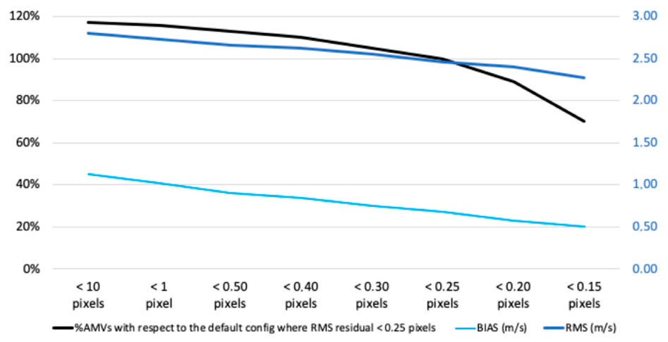
Additional refinements exist in the HRW algorithm to improve computational efficiency and retrieval fidelity. The tracking-window dimensions are dynamically determined based on the estimated displacement and the true inter-image time difference Δt, replacing the former static ~70 × 70 window with adaptive sizes typically near 42 × 42 pixels. This adjustment significantly reduces the computation time. Moreover, applying an internal filter of root mean square (RMS) residuals < 0.25 pixels within the HRW chain, prior to the standard quality control sequence, was found to yield slightly improved performance compared to applying the same criterion as a post-processing filter.
Considering the RMS residuals, a sensitivity analysis against ECMWF model analysis was performed. The results of this analysis show that the dependence is not too significant, as shown in Figure 9. The value of RMS residuals of <0.25 pixels was chosen because it defines a balance between the amount of AMV data and the corresponding reduction in errors.

3. Results

We exercised HRW to produce stereo and non-stereo AMVs for 24-h test cases from 00:00Z to 23:50Z, beginning 3 January 2025 and ending 28 March 2025 in 14-day steps. There are runs for each 10-min MTG-I/FCI FDHSI product time slot. Three types of examinations were undertaken. First, we made direct comparisons between the stereo and non-stereo height assignments. Second, we compared the AMVs with reanalysis winds from the ERA5 model. ERA5 reanalysis variables exist on a 0.25-degree grid, and the geopotential height is used as the vertical datum. Thirdly, we compared the AMV heights with Mie Attenuated Backscatter (MAB) curtains from the EarthCARE ATLID LiDAR. ERA5 and EarthCARE comparisons focus primarily on IR10.5 along LiDAR tracks, which enables all methods to be examined simultaneously day and night.

3.1. Direct Comparison of Stereo and Non-Stereo HRW Heights

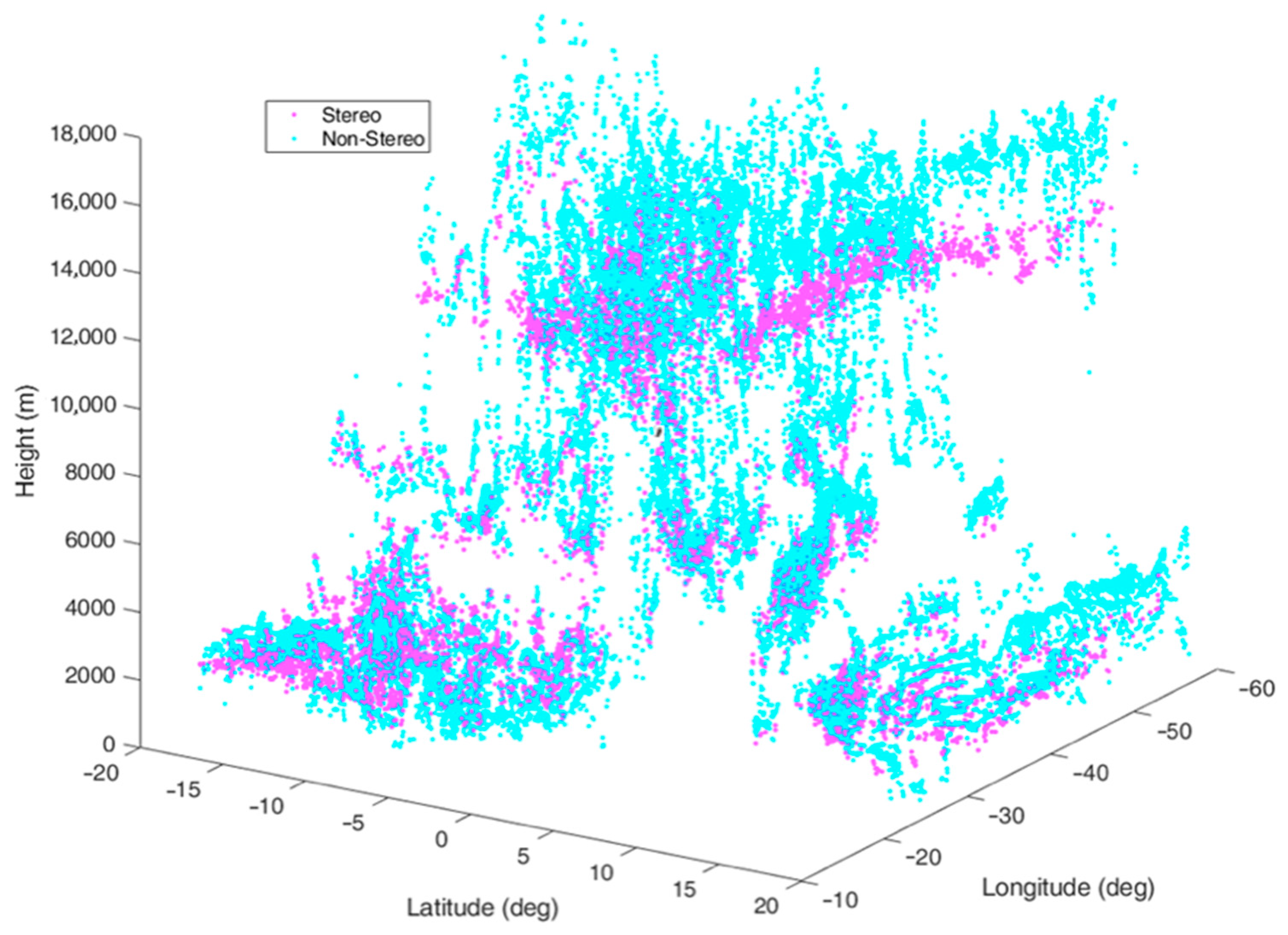
HRW tracks the same patterns regardless of the mode used for height assignment, which facilitates the collocations. The stereo mode generally produces fewer retrievals since additional high-quality matches are needed between the tracking templates from the FCI and the remapped ABI imagery for a stereo retrieval. The reduction is between 70% when three images are used and 90% when six images are used; the reduction for order 5 is larger than for order 3. As already shown in Figure 9, a second contributing factor is the additional quality screening applied to the stereo retrievals where the root-mean-square residual disparity needs to be less than 25% of a pixel. Figure 10 illustrates a typical comparison between the two height assignments in the tropics, which is where the largest differences are observed at upper levels. These differences can be larger than 1 km. Smaller height differences typically exist at lower levels. The implications of these differences are the main subject of our investigations.

3.2. HRW-ERA5-ATLID Comparisons

Cases where stereo and non-stereo AMVs are collocated along LiDAR curtains are a small subset of the full dataset, but important for comparing qualitatively observational winds to both LiDAR and reanalysis at the same time. In many cases, both stereo and non-stereo AMVs show similar results that align with both LiDAR and reanalysis. In other cases, there are significant differences, particularly at upper levels.
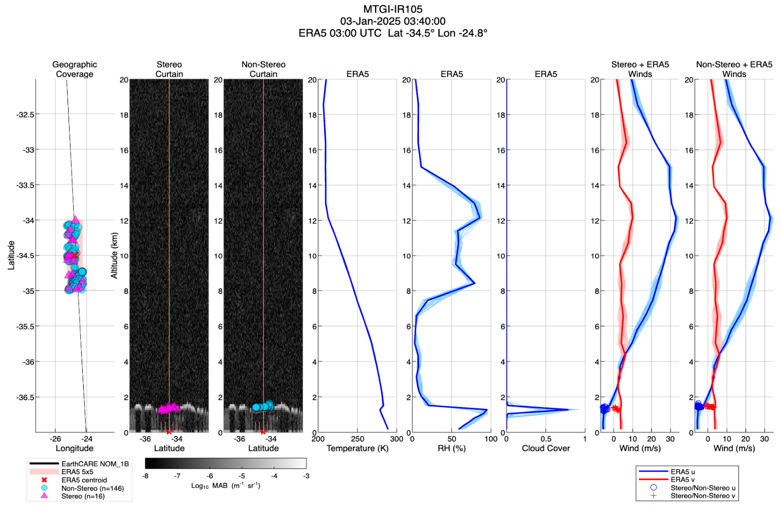
Figure 11 is an eight-panel display of a typical comparison where stereo and non-stereo AMVs are similar. The figure shows the path of the LiDAR curtain through a low-level cloud layer and a 5 × 5 box of ERA5 0.25° grid points. Both height assignment methods are quite consistent with the LiDAR representation of optically thick liquid-phase clouds. The five panels on the right show corresponding vertical profiles from ERA5. ERA5 layers are plotted by their geopotential heights rather than pressure levels to facilitate geometric comparison. The thick lines represent the center grid point, and the fainter lines show the other 24 grid points, indicating the spread of each variable across the 5×5 box. The rightmost panels are the wind profiles with the stereo and non-stereo AMVs overplotted. Non-stereo AMVs are assigned heights very close to the stereo assignments, even in the presence of a temperature inversion. Both sets of AMVs deviate from the reanalysis. It is likely that the observational AMVs are a better representation here of the atmospheric state than the reanalysis. The lack of perfect simultaneity between the observational AMVs and the reanalysis winds also plays a role.
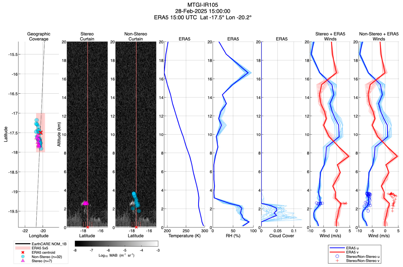
Figure 12 shows a case where a low-level non-stereo AMV calculation has gone wrong in the presence of a vanishing temperature lapse rate (vertical change in temperature with altitude). It is common for several non-stereo AMVs to occur near a stereo AMV, with some scattering in their heights around the height defined by the stereo AMV. In the case of big clouds, this can be understood through variations in the properties of the cloud (height and depth from the center to the edges), which are then reflected as variations in the heights of several non-stereo AMVs. However, in this specific case, the non-stereo AMVs deviate further from the reanalysis winds than they would have were they assigned the proper altitude. The ERA5 time is the same as the observational wind product time in this case.
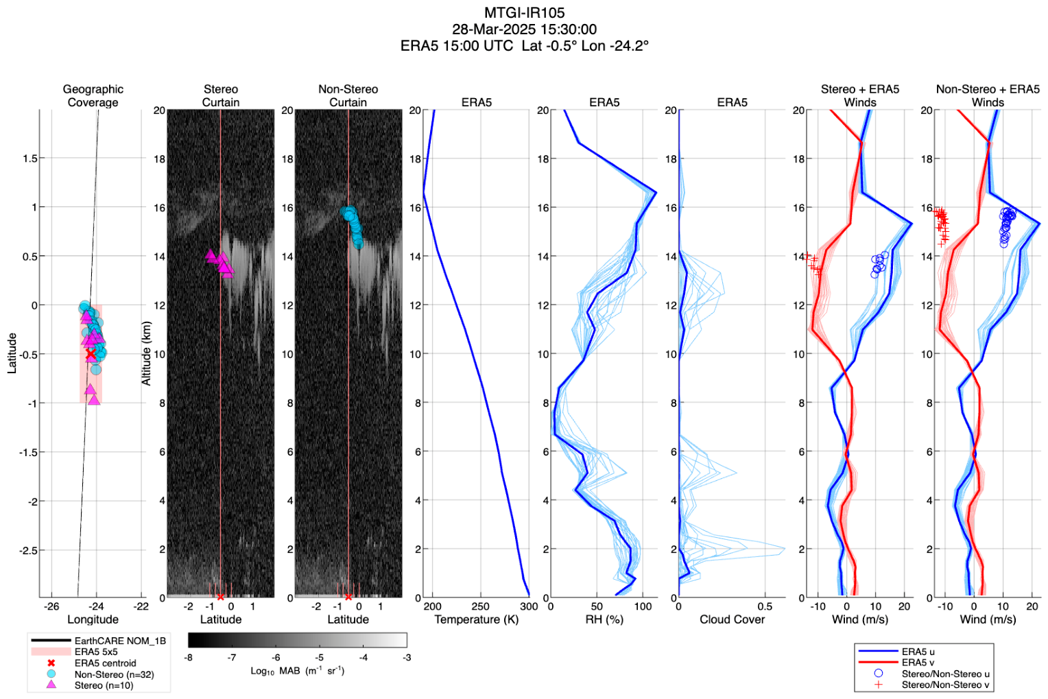
More dramatic differences can occur at high levels, as seen in Figure 13. In this example, the optically thick structure at ~13.5 km is clearly tracked by the stereo AMVs that align well with the reanalysis. On the other hand, the non-stereo AMVs define a similar displacement but have been assigned much higher values and so do not align well with the reanalysis. This is likely caused by the NWCSAF GEO-I Cloud outputs the non-stereo height assignment is based on, which define a higher cloud top in the presence of the higher transparent clouds at ~16 km which are not tracked by the AMV, as the non-stereo AMVs are essentially the same as the stereo ones raised ~2 km higher in the atmosphere. The consequence of height assignment error depends of course on the amount of wind shear (change in wind with altitude) present. In the absence of shear, the observational AMV is correct regardless of height assignment.
Even though such triple comparisons are possible only along a LiDAR curtain, the LiDAR is quite useful for showing the altitudes of trackable features case by case. There are 797 plots showing the stereo and non-stereo AMVs against LiDAR and the reanalysis available for comparison, as later explained in the “Supplementary Materials.” In this collection, we have interpolated the reanalysis winds to the assigned height in each case and calculated the vector difference with the observed wind. There are 134 cases that have adequate numbers of both stereo and non-stereo collocated winds (defined as >10, a value that characterizes an empirical compromise between sample availability and representativeness).
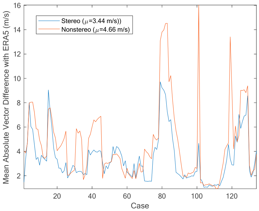
The Mean Absolute Vector Difference (average of V u + V v ) with the reanalysis winds are shown in Figure 14 for such cases. We note that the non-stereo cases typically deviate more from the reanalysis than do the stereo cases; however, both exhibit instances where there are large deviations from the reanalysis, probably indicating that the reanalysis is not correctly representing the atmospheric state at that place and time. The differences between observed and collocated, height-interpolated reanalysis winds are 3.44 m/s for stereo height assignment and 4.66 m/s for non-stereo height assignment when averaged over all cases.
A benefit of LiDAR is that it qualitatively indicates how well the HRW stereo heights correlate with cloud tops, taking into account that the method used by both processes to detect the cloud tops is very different (passively from visible or infrared satellite images, or actively processing the LiDAR signal). Many figures in the “Supplementary Materials” show a similar behavior: the HRW stereo heights correlate well with the apparent LiDAR cloud tops in thin clouds at all levels, although the HRW stereo heights can be slightly higher at the low levels and slightly lower at the high levels occasionally. In thick clouds, the situation becomes different, and the HRW stereo heights tend to correlate with a level in the middle of the cloud MAB profile. With high transparent clouds over lower opaque clouds, the HRW stereo heights correlate in the infrared channel with the lower opaque clouds.

3.3. ERA5-HRW Comparisons

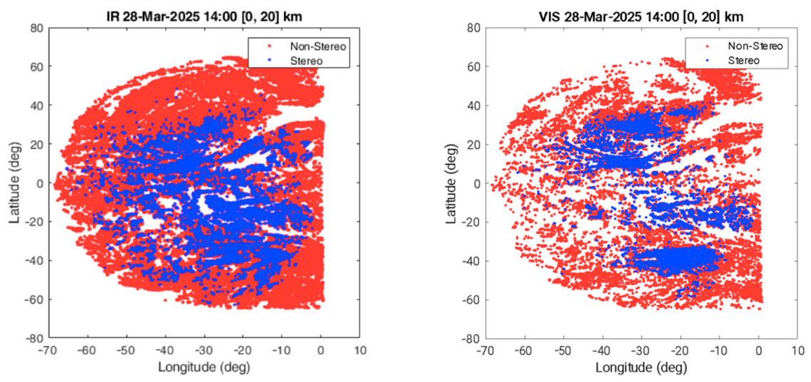
The global reach of ERA5 reanalysis allows a broader comparison between observational AMVs and reanalysis winds once freed from the need to collocate with a LiDAR curtain. Figure 15 shows an example of the geographic range of infrared and visible winds of each type from 28 March 2025 14:00Z. Non-stereo winds populate the western half of almost a full hemisphere. Stereo winds populate most of the overlap of the two satellite images, but less densely than the non-stereo ones, particularly for the visible winds. It is noon at −30° longitude and mid-morning at the western edge, where there remain many non-stereo wind sites and few stereo ones. In general, the stereo winds thin near the extremities of the overlap region for all winds and near the terminator region for the visible winds, as the viewing geometry from the respective satellites becomes less similar and the footprints of pixels elongate.
In this analysis, we look for the stereo and non-stereo winds to compare with ERA5 at the top of each hour. There are sometimes missing slots when subsequent 10-min slots are tried. The result, in all cases, is that the selected stereo and non-stereo HRW are simultaneous and equally displaced in time from ERA5. Next, we identify all winds of each type collocated within ±0.125° in latitude and longitude of each ERA5 grid site. When there are winds of both types found for a site, we compare the one wind of each type nearest the ERA5 grid site with the ERA5 wind interpolated to the respective height assignment. There is no interpolation of ERA5 in space or time except for the interpolation of the wind in the vertical column with the geopotential height as the vertical datum, which reduces uncertainty that could arise from spatial gradients or temporal evolution.
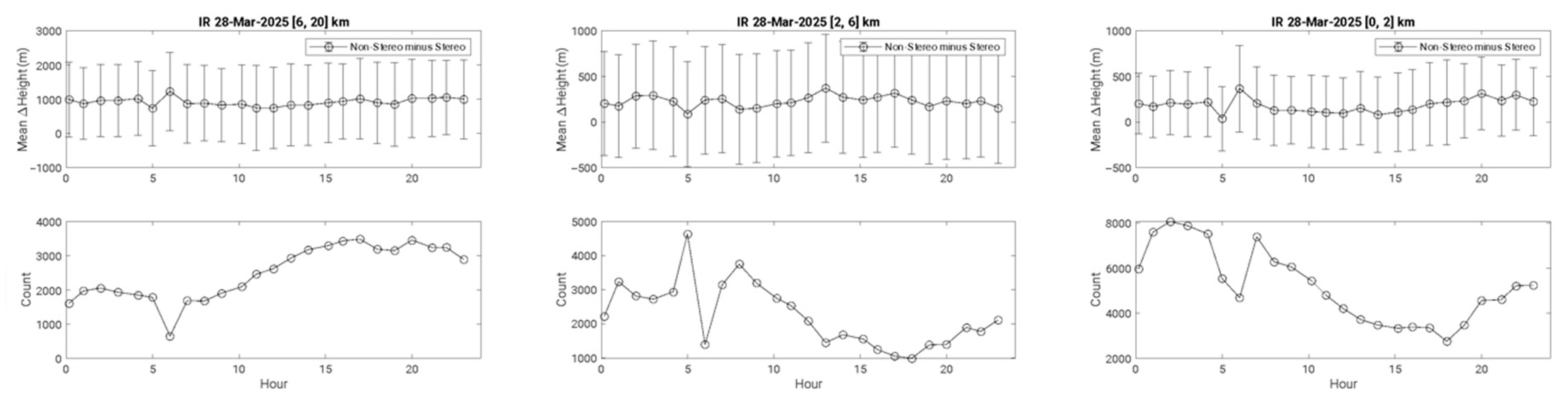
With stereo, non-stereo, and ERA5 winds all effectively collocated, we can compare both stereo and non-stereo results to ERA5 without favoring one or the other. Figure 16 shows the mean difference in height assignment with the standard deviation as error bars and counts of such triply collocated data points for each hour of one day (28 March 2025). Winds have been divided into high (>6 km), mid (2–6 km), and low levels (<2 km) according to the stereo height (from left to right). There could be cases where a stereo wind belongs to one level, but a very close neighboring non-stereo wind clearly belongs to another. In such a case, the height difference would be anomalous because the two winds belong to different layers; both could be equally correct, just different winds that belong in different layers and should not be compared. We try to exclude such situations by not counting either type of wind when the non-stereo wind is more than 1 km outside the level to which the stereo wind belongs. These are relatively few, and including or excluding these cases has almost no impact on the results.
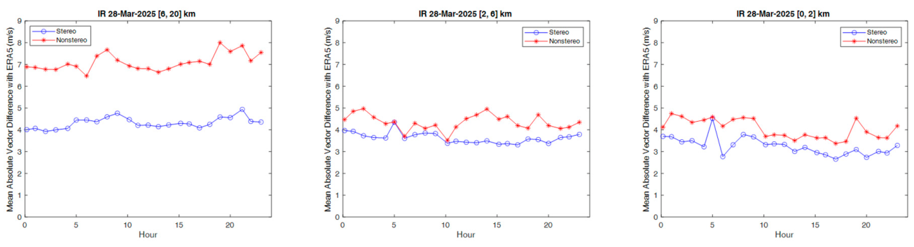
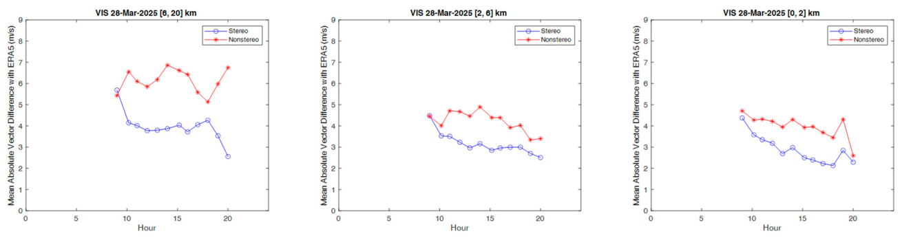
We can observe that the non-stereo heights are on average uniformly higher than the stereo heights. Therefore, we should expect that the comparisons with the ERA5 winds will be different in the two cases. This comparison is shown in Figure 17 for the infrared winds, where we can observe that the stereo winds are closer to the ERA5 winds. The difference is most important at high levels and less at the mid- and low levels. The same pattern is seen for the visible winds in Figure 18 when there is sufficient illumination to produce a visible image. In general, the visible differences with respect to ERA5 are smaller than the infrared differences for both types of winds, and more significantly for the stereo winds. This may be indicative of visible winds being more accurate because of the higher resolution of the visible channel, which improves the results for both methods.
The comparisons for the other dates tested are similar to those shown for 28 March 2025 above (plots for all dates are in the Supplementary Materials). Table 1 provides a summary of daily statistics stratified by level for each band and test date. We report the difference in height assignments, showing that the non-stereo height assignments are consistently higher than the stereo assignments. The height assignment differences lead to different wind velocities interpolated along the ERA5 vertical profile for the comparison. The stereo method consistently exhibits better agreement with ERA5 winds at high levels according to all metrics. These are Mean Absolute Vector Difference (MAVD), Mean Vector Difference (MVD), and Root Mean Square Vector Difference (RMSVD). MAVD, already introduced, is the average of V u + V v . MVD is the average of V u 2 + V v 2 , and RMSVD is the root-mean-square average of the same. The differences are less pronounced for the mid- and low-level winds, but still generally favor the stereo method. Statistics are aggregated across the full population for the date and level, with the population count given for each.

4. Discussion

In the evaluated datasets, we observe better quantitative agreement of stereo winds relative to ERA5. The most pronounced distinctions emerge at high levels (>6 km) where the height assignments differ the most; but at all levels, the non-stereo height assignments are higher than those of stereo on average. These observations can be explained with the stereo height assignments being more accurate than the non-stereo ones, indicating a benefit to improving the non-stereo assignments, especially at high levels.
Considering the mean RMSVD for all days in Table 1, we can see that it is at least 40% smaller for high-level stereo AMVs and at least 10% smaller for both medium and low-level stereo AMVs.
The comparisons with ERA5 along LiDAR traces show, in many cases, qualitative errors in the height assignment by the non-stereo AMVs, with a lack of clear evidence of trackable features in the LiDAR curtains, most probably related to the NWCSAF GEO-I Cloud outputs they are based on. The stereo height assignment appears more consistent with LiDAR/ERA5 in these cases.
In both cases, the size of the evaluated datasets is limited, and so the stratification of the results for different cloud types and geographical regions was not done, which could have some impact on the generality of the current conclusions.
Considering the operational implications of using the stereo AMVs with MTG-I and GOES-East, the stereo method can only be applied over less than half of the MTG-I full-disk pixels (as shown, for example, in Figure 15). Additionally, the stereo mode produces fewer AMVs since additional high-quality matches are needed from both FCI and ABI imagery for stereo retrieval. The reduction is between 70% and 90%. Considering processing time, the amount added for the stereo processing is small, and the added processing time for stereo AMVs is offset by their lower numbers.
For operational use by the NWCSAF users, the HRW product inside the NWCSAF GEO-I v2027 software package will have the option to include both stereo AMVs and non-stereo AMVs, and each will have its own “Quality indicator” values considering their specific height/pressure values. With this, an assimilation strategy would be simple: use and assimilate non-stereo AMVs in locations where stereo AMVs are not available, and use and assimilate the AMVs with better “Quality indicator” values in places where both are available. With this simple procedure, we are not missing any information previously available when only non-stereo AMVs were calculated, and we are resolving the question of which of the stereo or non-stereo AMVs is better in each location (as in general it has been seen for many years that the quality of the AMVs is better with higher “Quality indicator values”). Alternatively, for a tracer where we can calculate both stereo and non-stereo AMVs, we can define an additional quality check that compares the “Quality indicator” for both and rejects both if the difference is over a defined threshold (due to the discrepancy between both AMVs).
It is here necessary to remark, however, that the AMV best-fit level (defined as the pressure level at which the horizontal wind defined by the AMV fits best with the wind defined by any reference observation, like a NWP wind analysis or a radiosounding wind profile) does not necessarily relate to the highest opaque cloud-top level (which is the pressure level defined by the stereo method and also by CCC method using CTTH product as input), as several studies have already shown [26,27,28], and which HRW itself has evaluated through the correction in the AMV level based on the cloud depth, represented by the liquid/ice water path obtained from the Cloud Microphysics product (explained in [1], chapter 2.4.3, pp 14–17). This correction locates, in general, the AMV best-fit level in a level below this cloud top, nearer to the ground, except for AMVs with very small ice/liquid water path values. The difference between both pressure values increases approximately linearly with the liquid/ice water path.
Due to this, the relationship between the stereo height (related to the optimal calculation of this cloud top through a geometrical procedure), the CCC method non-stereo height (related to the calculation of the same cloud top through physical considerations) and the AMV best-fit height implies additional studies based on the different behavior considering different satellite channels, cloud types, cloud heights and cloud depths.
Plans have already been defined inside NWCSAF during the following phase (2027–2032) to better relate the stereo height, the alternative CCC height, the cloud-top height and the AMV best-fit height for AMVs related to the different cloud types with the use of larger validation datasets and with the objective of improving the CCC height assignment method, which can be used anywhere without the geometric limitations of the stereo method. These additional studies will consider, for example, the EarthCARE ATLID L2 cloud-layer height product as a reference for cloud-top height or the height of significant backscatter layers for the AMVs related to the different cloud types, to calculate corresponding statistics and error distributions. Here it is clear, however, that the relationship between all these variables can be different for the different cloud types, and the conclusions can be different for the different cloud types. The additional studies would also include examination of cloudy and clear-sky water vapor winds, which were left unexamined in the present study in favor of window-channel infrared and visible winds, and would improve the quantity of stereo retrievals without significantly compromising their quality.
Additionally, while the ERA5 comparison results are interesting, we must ask if conformance with reanalysis should be the standard against which to judge the correctness of the observed AMVs, or whether we are engaging in a sort of circular reasoning. Numerical models such as ERA5 assimilate operational AMVs from European, American and Japanese geostationary and polar satellites, distinct from HRW, with diverse NWP-dependent height assignment methods related to the AMV temperature [29], but their modeling of the atmosphere might be expected to be influenced by whatever errors or biases that might exist in these operational height assignments.

5. Conclusions

The quantitative and qualitative comparisons shown in this paper indicate the potential benefit of stereo height assignment relative to the non-stereo “Cross Correlation Contribution (CCC)” method, as implemented in HRW, to accurately represent the state of the atmosphere.
The “stereo height assignment method” implemented in the HRW product will be available to NWCSAF users inside the following software package version (NWCSAF GEO-I v2027), to be released in 2027, and will support additional studies to improve the existing non-stereo height assignment methods, based on the different behavior of corresponding stereo and non-stereo AMVs for the different satellite channels, cloud types, cloud heights and cloud depths.

Supplementary Materials

Supplementary Materials are available for download as Friberg, M.D.; Carr, L.C.; Madani, H.; García-Pereda, J.; Wu, D.L.; Lei X. (2026) NWCSAF GEO-I High Resolution Winds stereo and non-stereo AMV curtain-plot comparisons with EarthCARE and ERA5 over the Atlantic Ocean. Dryad Dataset: https://doi.org/10.5061/dryad.qbzkh190b. They include the 797 plots (figures) defined in Section 3.2 and a complete set of comparisons with ERA5 defined in Section 3.3. The MATLAB R2024B code to make these plots and aggregate statistics from the HRW output is accessible here too.

Author Contributions

Conceptualization and methodology, J.L.C.; Software, J.G.-P., J.L.C., X.L. and M.D.F.; Validation, J.L.C., M.D.F., H.M. and X.L.; Formal analysis, J.L.C., M.D.F., H.M. and X.L.; Writing—original draft preparation, J.L.C., J.G.-P., M.D.F., H.M. and X.L.; Writing—review and editing, J.L.C., J.G.-P., M.D.F., H.M., X.L. and D.L.W.; Funding acquisition, J.G.-P., D.L.W., M.D.F. and J.L.C. All authors have read and agreed to the published version of the manuscript.

Funding

This research is funded by the “European Organisation for the Exploitation of Meteorological Satellites (EUMETSAT)” through the “Satellite Application Facility on Support to Nowcasting and Very Short Range Forecasting (NWCSAF)” and its “Fourth Continuous Development and Operations Phase (CDOP-4, 2022–2027)” Visiting Scientist Activity (VSA) program, and by the “National Aeronautics and Space Administration (NASA)” under the “Support for Atmospheres, Modeling, and Data Assimilation (SAMDA)” contract NNG17HP01C at Goddard Space Flight Center. The Article Processing Charge (APC) is funded by “Agencia Estatal de Meteorología (AEMET),” also with funds coming from EUMETSAT for the NWCSAF.

Data Availability Statement

The updated HRW product (including the whole stereo processing module and all needed LUTs and auxiliary data) will be released to registered NWCSAF users in early 2027 inside the following software package version (NWCSAF GEO-I v2027), once it is approved by the NWCSAF Steering Group. As there are no general restrictions to becoming an NWCSAF user, the HRW algorithm and the NWCSAF GEO-I v2027 software package can thus be considered free of charge after the corresponding license acceptance, and any interested person will have the option to test it and use it once it becomes available.

Acknowledgments

The authors want to acknowledge the financial support from the involved institutions, without which this study would not have been possible. The authors also want to acknowledge Pilar Rípodas, Project Manager of the NWCSAF in AEMET, for her work related to the administration and funding acquisition, without which this study would not have been possible either.

Conflicts of Interest

Authors James L. Carr, Houria Madani and Xuming Lei were employed by the company Carr Astronautics Corporation. The remaining authors declare that the research was conducted in the absence of any commercial or financial relationships that could be construed as a potential conflict of interest.

Abbreviations

The following abbreviations are used in this manuscript:
3-Dthree-dimensional
ABIGOES-R Advanced Baseline Imager
AEMETAgencia Estatal de Meteorología of Spain
AMVAtmospheric Motion Vector
ATBDAlgorithm Theoretical Basis Document
EUMETSATEuropean Organisation for the Exploitation of Meteorological Satellites
CCCCross Correlation Contribution height assignment method for AMVs
CMICNWCSAF GEO-I and PPS Cloud Microphysics product
CTNWCSAF GEO-I and PPS Cloud Type product
CTTHNWCSAF GEO-I and PPS Cloud Top Temperature and Height product
EarthCAREEarth Cloud, Aerosol and Radiation Explorer (European/Japanese mission)
ECMWFEuropean Centre for Medium-Range Weather Forecasts
ERA5ECMWF’s Atmospheric Reanalysis of the Global Climate, Version 5
FCIMTG-I Flexible Combined Imager
FDHSIMTG-I/FCI Full-Disk High Spectral Resolution Imagery
GEO, GEO-IGeostationary
GOES-EastNOAA’s GOES satellite positioned over the equator at 75.2° West longitude
GOES-RNOAA’s Third-Generation Geostationary Operational Environmental Satellites
GSFCNASA’s Goddard Space Flight Center
Himawari-8/9 JMA’s Himawari Third generation of geostationary satellites
HRWNWCSAF GEO-I and PPS High Resolution Winds AMV product
INRImage Navigation and Registration
IRInfrared channel in a meteorological satellite imager
JMAJapan Meteorological Agency
JPSSNASA/NOAA’s Joint Polar Satellite System
LUTLook-Up Table
MABEarthCARE’s Mie Attenuated Backscatter
MAVDMean Absolute Vector Difference
MTGEUMETSAT’s Meteosat Third-Generation Satellites
MTG-IEUMETSAT’s Meteosat Third-Generation Satellites Imager
MVDMean Vector Difference
NASAUnited States National Aeronautics and Space Administration
NetCDFNetwork Common Data Format
NOAAUnited States National Oceanic and Atmospheric Administration
NWCSAFEUMETSAT’s Satellite Application Facility on Support to Nowcasting and Very Short Range Forecasting
NWCSAF/GEO-INWCSAF software package for geostationary satellites
NWCSAF/PPSNWCSAF software package for polar satellites
NWPNumerical Weather Prediction
RMSRoot Mean Square
RMSVDRoot Mean Square Vector Difference
SatAReference satellite in the stereo process
SatBSecondary satellite in the stereo process
VIIRSJPSS Visible Infrared Imaging Radiometer Suite
VISVisible channel in a meteorological satellite imager
VRValidation Report
WVWater vapor channel in a meteorological satellite imager

Appendix A

Stereo Wind Retrieval Algorithm
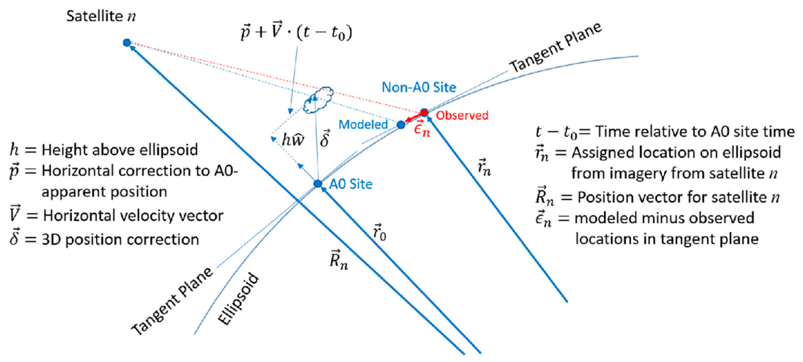
The stereo wind retrieval is an optimization problem using the apparent locations of a tracer on the ellipsoid, as observed by MTG-I/FCI and GOES-R/ABI radiometers at various times. One of the scenes is designated to be the “reference” scene from which the tracking template is taken. We designate it as the “A0” scene. Other repetitions from the same satellite are designated “A1,” “A2,” etc. The other satellite is designated as the “B” satellite. For the NWCSAF GEO-I HRW algorithm, the reference scene “A0” will be from FCI, and the “B” scenes are from ABI (in a parallel NASA implementation, the roles of FCI and ABI are swapped). The apparent location of the tracer on the ellipsoid and a time tag for its acquisition in each scene will have been found already by the original tracer tracking process of the HRW algorithm.
The mathematics of the retrieval algorithm is explained with reference to Figure A1. It shows the view of a tracer from a satellite n ( n = 0 is A0, n 0 are A1, B0, B1, etc.) with position vector R n . The apparent location r 0 of the tracer on the ellipsoid as seen in A0 is marked. The three-dimensional location of the tracer relative to this point on the ellipsoid is δ , which can be decomposed into a horizontal distance the wind ( V ) has carried it in the time t n t 0 and a vertical height h w ^ . The unit vector w ^ is perpendicular to the tangent plane at A0 and V · w ^ = 0 . The apparent location r n of the tracer on the ellipsoid as observed by satellite n 0 is similarly marked.
Figure A1. Geometry for the retrieval algorithm.
Remotesensing 18 02940 g0a1
The optimization problem seeks to minimize the sum of the weighted squared deviations between the modeled and observed apparent locations of the tracer across all scenes. This is expressed mathematically in Equation (A1).
χ 2 = n = 1 N ϵ n T W n ϵ n
The weighting matrices W n will be taken to be diagonal with the diagonal elements being inverse to the assumed errors in measurement ( = 1 σ 2 ). The residual displacements ϵ n are in the tangent plane at the site of each observation and represent the distance between the observed and modeled apparent sites.
Two models are supported. The first is a three-parameter model X = h , V   T and the second is a five-parameter model X = p , h , V   T . In the first case, the vector δ is constrained so that it points from the apparent site A0 to the A0 satellite (i.e., along its line of sight). In the second case, the apparent position of A0 can be adjusted in the tangent plane, supposing that there may have been a small error in the Image Navigation and Registration (INR) of the A0 satellite. Such an INR error will be absorbed into p ; otherwise, it will find its way into the residuals.
The problem is mildly nonlinear in X , and solved iteratively, where at each step a change X is computed from a linearized version of the problem. The iteration is stopped when certain convergence criteria are met, or the maximum number of allowable loops has been attempted without converging (failure). The convergence can also fail in the pathological case where applying p for the next iteration would put the tracer over the horizon or too close to the limb of one of the satellites (rare occurrence). Below, we describe and derive each step of this process, which has been implemented in the HRW product.
The general solution to this kind of problem is as follows. Given a guess X , we imagine an updated guess X + X and expand each ϵ n as a Taylor series to linear order in X as in Equation (A2).
χ 2 n = 1 N ϵ n X + A n · X T W n ϵ n X + A n · X
The matrix A n is the 2-by-3 (or 2-by-5) matrix of partial derivatives of ϵ n with respect to each component of X . Each update is calculated to minimize χ 2 . We find this minimum by differentiating χ 2 with respect to the X and setting that to zero. The result is a linear system of equations that can be solved using any standard linear algebra method, as in Equation (A3).
n = 1 N A n T W n A n · X + n = 1 N A n T W n ϵ n X = 0
A necessary condition for the coefficient matrix to be nonsingular and for there to be a unique solution is that the number of scalar measurements exceeds the number of parameters being solved. Each pairing, A1-A0, A2-A0, B0-A0, etc., contributes two scalar measurements as ϵ n sits in a two-dimensional tangent plane; therefore, we need to have 2 N > 3 or 2 N > 5 , counting zero as the reference scene. The loop is terminated when the norm of the position components of X and the norm of the velocity components of X are both less than specified tolerances.
It remains to describe the calculations of ϵ n and A n . The first term on the right in Equation (A4) is a vector to the tracer with a scale factor λ > 1 applied such that it extends towards the surface from the n = 0 satellite. The second term is a vector from satellite n 0 to the observed apparent location of the tracer.
ϵ n = λ r 0 + δ R 0 r n R n
Since ϵ n is to be in the tangent plane at r n , it must be perpendicular to the local vertical w ^ n there, i.e., w ^ n · ϵ n = 0 , which is a condition that allows us to solve for λ in Equation (A5).
λ = w ^ n   · r n R n w ^ n   · r 0 + δ R 0
Therefore,
ϵ n = w ^ n   · r n R n w ^ n   · r 0 + δ R 0 r 0 + δ R 0 r n R n
The vector δ is parameterized by either five or three independent variables X :
δ ( X ) =   p + h w ^ 0 + V · t n t 0   X = p , h , V   T h · R n r 0 w ^ 0 · R n r 0 + V · t n t 0   X = h , V   T
We substitute these definitions directly in Equation (A6) to calculate ϵ n ( X ) and to also find the matrix of partial derivatives A n for the two cases:
A n = w ^ n   · r n R n w ^ n   · r 0 + δ R 0 I r 0 + δ R 0 w ^ n   · r 0 + δ R 0   w ^ n T δ X
The position vector calculations are coded in a geographic frame where the xy-plane is the equator and the x-axis is at the Greenwich Meridian; however, we wish to represent the winds in a local coordinate system at r 0 where the frame is defined by a triad of unit vectors that are respectively east-pointing (u, zonal), north-pointing (v, meridional), and vertical (w). We define a matrix M 0 = u ^ 0   v ^ 0   w ^ 0 , with each column being a triad vector in the geographic frame, that transforms the vector components from the local tangent frame into the geographic frame. The matrix M 0 T does the inverse. In the two parameterizations (recall that V · w ^ = 0 in our model)
δ X = u ^ 0   v ^ 0     w ^ 0   t n t 0 u ^ 0   t n t 0 v ^ 0 R n r 0 w ^ 0 · R n r 0   t n t 0 u ^ 0   t n t 0 v ^ 0
The linear system in Equation (A3) expressed in the local tangent frame is, therefore
n = 1 N M 0 T A n T W n A n M 0 · X = n = 1 N M 0 T A n T W n b n b n = ϵ n X X = p u   p v   h   V u   V v T h   V u   V v T
When the weights relate approximately to the uncertainty of the measurements, the coefficient matrix n = 1 N A n T W n A n can be useful to estimate the uncertainty for the retrieved variables in accordance with least-squares fitting theory (e.g., Gibbs, 2011 [30]). We can see this easily by assuming that we have a solution under perfect conditions and then we add noise so that each b n is a pair of zero-mean random numbers with covariance c o v b n = R n . Let us assume independence across n , and calculate the expectation values ( E   ·   ) across an ensemble of trials using Equations (A10).
First, calculate
E n = 1 N M 0 T A n T W n A n M 0 · X = n = 1 N M 0 T A n T W n A n M 0 · E X                 = E n = 1 N M 0 T A n T W n b n = n = 1 N M 0 T A n T W n E b n = 0
From which we conclude that E X = 0 , so the distribution of retrieval errors is zero mean. Now consider the second order statistic E X · X T . We take advantage of the symmetry of the matrices and the assumed independence of the measurements, so that E b n b m T is nonzero only when n = m , i.e., E b n b m T = R n , and calculate
E X · X T = n = 1 N M 0 T A n T W n A n M 0 1 · E n = 1 N M 0 T A n T W n b n · n = 1 N M 0 T A n T W n b n T · n = 1 N M 0 T A n T W n A n M 0 T 1                                 = n = 1 N M 0 T A n T W n A n M 0 1 n = 1 N M 0 T A n T W n R n W n A n M 0 n = 1 N M 0 T A n T W n A n M 0 1
Now, if we had selected W n = R n 1 then Equation (A12) reduces to the statement that the covariance of the retrieval uncertainty is the inverse of the coefficient matrix of Equation (A10).
c o v X = E X · X T = n = 1 N M 0 T A n T W n A n M 0 1
The uncertainties on each retrieved parameter individually would be the square root of the diagonal elements of c o v X .
We remarked earlier that it is necessary to have 2 N > 3 or 2 N > 5 , in the three- or five-parameter model, where N is the number of scenes other than the reference one. The overdetermination is then either 2 N 3 or 2 N 5 . Overdetermination is generally a good thing in fitting problems if random measurement errors were the only factor to consider. However, there is an implicit assumption in satellite winds that the tracer is only translating. This assumption is best respected when the time between observations is least but then that makes the translation smaller and harder to distinguish from noise. If we continue to add extra scenes for more overdetermination then the assumption becomes less well respected, so there is a tradeoff.
There are several obvious configurations that can work. With the three-parameter model, we can have as few as three scenes ( N = 2 ) , e.g., (A0, A1, B0) or (A0, B0, B1) that move only one time stamp from A0. With the five-parameter model, we need at least four scenes e.g., (A0, A1, B0, B1). Both cases are overdetermined by only one. In the three-parameter case, there is no loss in treating the A and B satellites equivalently, so (A0, A1, B0, B1) is a better choice. This configuration would be overdetermined by three. In the five-parameter case, it would seem that we would pay a penalty against the translation assumption by adding scenes; however, this need not be the case. Consider (A0, A1, A2, B0, B1, B2), which is overdetermined by five, where A0 is slot T , A1 is slot T T , and A2 is slot T + T , and similarly for the B satellite with repeat period T . Since all matches are against a tracer template from A0, they are never further than T away. This is the usual configuration chosen for the NASA research code, the preoperational NOAA code, and the implementation in HRW code. The penalty is that the AMVs are produced one slot behind in a real-time system. Even with (A0, A1, A2) and (B0, B1, B2) ordered backwards in time, the benefit of overdetermination is an incentive for using six scenes. There is no reason that this configuration could also not apply to the three-parameter model.
In general, we prefer the five-parameter model because INR errors (the geographic assignments to the A0 tracers) are generally systematic. Such errors would find their way into the residuals, and we would like the residuals to be noise-like. Noise-like residuals can be used for testing whether the data being fit is likely conforming to the model (i.e., the tracer translates as it moves in the wind and the parallax observed is related to the height). If the measurement errors were simply Gaussian then the mean-squared statistics of the residuals would be expected to be χ -squared with degrees of freedom equal to the overdetermination. The real world is more complicated, and we do not exactly know the underlying distribution; however, we can empirically make it from the ensemble of all wind retrievals. Some experimentation can determine what threshold to apply to the root-mean-squared residual to screen out cases that are possibly nonconforming with the model from erroneous matches or other reasons.

References

  1. García-Pereda, J.; Fernández-Serdán, J.M.; Alonso, Ó.; Sanz, A.; Guerra, R.; Ariza, C.; Santos, I.; Fernández, L. NWCSAF High Resolution Winds (NWCSAF GEO-I HRW) Stand-Alone Software for Calculation of Atmospheric Motion Vectors and Trajectories. Remote Sens. 2019, 11, 2032. [Google Scholar] [CrossRef] [Scilit]
  2. García-Pereda, J. Algorithm Theoretical Basis Document for “High Resolution Winds” for Geostationary Satellites (NWCSAF GEO-I HRW v2025); NWCSAF/AEMET: Madrid, Spain, 2025. [Google Scholar] [CrossRef]
  3. García-Pereda, J. Algorithm Theoretical Basis Document for “High Resolution Winds” for Polar Satellites (NWCSAF PPS HRW v2021.3); NWCSAF/AEMET: Madrid, Spain, 2022. [Google Scholar] [CrossRef]
  4. García-Pereda, J. Validation Report for “High Resolution Winds” for Geostationary Satellites (NWCSAF GEO-I HRW v2025); NWCSAF/AEMET: Madrid, Spain, 2025. [Google Scholar] [CrossRef]
  5. García-Pereda, J. Validation Report for “High Resolution Winds” for Polar Satellites (NWCSAF PPS HRW v2021.3); NWCSAF/AEMET: Madrid, Spain, 2022. [Google Scholar] [CrossRef]
  6. Velden, C.S.; Bedka, K.M. Identifying the uncertainty in determining satellite-derived atmospheric motion vector height attribution. J. Appl. Meteorol. Climatol. 2009, 48, 450–463. [Google Scholar] [CrossRef] [Scilit]
  7. Borde, R.; Oyama, R. A direct link between feature tracking and height assignment of operational AMVs. In Proceedings of the 9th International Winds Workshop, Annapolis, MD, USA, 14–18 April 2008; Available online: https://cgms-info.org/html/IWW09_PROC/groups/cps/documents/document/pdf_conf_p51_s3_13_borde_v.pdf (accessed on 17 August 2026).
  8. Purdom, J.F.W.; Dills, P.N. Cloud motion and height measurements from multiple satellites including cloud heights and motions in polar regions. In Proceedings of the 2nd International Winds Workshop, Tokyo, Japan, 13–15 December 1993; Available online: https://cgms-info.org/html/iww2/p245-248_Purdom-Cloud%20Motion.pdf (accessed on 17 August 2026).
  9. Carr, J.L.; Daniels, J.; Wu, D.L.; Bresky, W.; Madani, H.; Friberg, M.D.; Summers, T.C. Advances in stereo winds. In Proceedings of the 16th International Winds Workshop, Montreal, QC, Canada, 8–12 May 2023; Available online: https://cgms-info.org/html/iww16_html/session2/Monday_1430_IWW16_Jim_Carr.pdf (accessed on 17 August 2026).
  10. Carr, J.L.; Wu, D.L.; Daniels, J.; Friberg, M.D.; Bresky, W.; Madani, H. GEO–GEO Stereo-Tracking of Atmospheric Motion Vectors (AMVs) from the Geostationary Ring. Remote Sens. 2020, 12, 3779. [Google Scholar] [CrossRef] [Scilit]
  11. Carr, J.L.; Wu, D.L.; Kelly, M.A.; Gong, J. MISR-GOES 3D Winds: Implications for Future LEO-GEO and LEO-LEO Winds. Remote Sens. 2018, 10, 1885. [Google Scholar] [CrossRef] [Scilit]
  12. Carr, J.L.; Wu, D.L.; Wolfe, R.E.; Madani, H.; Lin, G.; Tan, B. Joint 3D-wind retrievals with stereoscopic views from MODIS and GOES. Remote Sens. 2019, 11, 2100. [Google Scholar] [CrossRef] [Scilit]
  13. Carr, J.L.; Wu, D.L.; Friberg, M.D.; Summers, T.C. Multi-LEO satellite stereo winds. Remote Sens. 2023, 15, 2154. [Google Scholar] [CrossRef] [Scilit]
  14. Carr, J.L.; Horváth, Á.; Wu, D.L.; Friberg, M.D. Stereo plume height and motion retrievals for the record-setting Hunga Tonga-Hunga Ha’apai eruption of 15 January 2022. Geophys. Res. Lett. 2022, 49, e2022GL098131. [Google Scholar] [CrossRef] [Scilit]
  15. Horváth, Á.; Carr, J.L.; Girina, O.A.; Wu, D.L.; Bril, A.A.; Mazurov, A.A.; Melnikov, D.V.; Hoshyaripour, G.A.; Buehler, S.A. Geometric estimation of volcanic eruption column height from GOES-R near-limb imagery—Part 1: Methodology. Atmos. Chem. Phys. 2021, 21, 12189–12206. [Google Scholar] [CrossRef] [Scilit]
  16. Horváth, Á.; Girina, O.A.; Carr, J.L.; Wu, D.L.; Bril, A.A.; Mazurov, A.A.; Melnikov, D.V.; Hoshyaripour, G.A.; Buehler, S.A. Geometric estimation of volcanic eruption column height from GOES-R near-limb imagery—Part 2: Case studies. Atmos. Chem. Phys. 2021, 21, 12207–12226. [Google Scholar] [CrossRef] [Scilit]
  17. Horváth, Á.; Carr, J.L.; Wu, D.L.; Bruckert, J.; Hoshyaripour, G.A.; Buehler, S.A. Measurement report: Plume heights of the April 2021 La Soufrière eruptions from GOES-17 side views and GOES-16–MODIS stereo views. Atmos. Chem. Phys. 2022, 22, 12311–12330. [Google Scholar] [CrossRef] [Scilit]
  18. Muth, L.J.; Bierbauer, S.; Hoose, C.; Vogel, B.; Vogel, H.; Hoshyaripour, G.A. Influence of Fire-Induced Heat and Moisture Release on Pyro-Convective Cloud Dynamics During the Australian New Year’s Event: A Study Using Convection-Resolving Simulations and Satellite Data. Atmos. Chem. Phys. 2025, 25, 16027–16040. [Google Scholar] [CrossRef] [Scilit]
  19. Friberg, M.D.; Wu, D.L.; Carr, J.L.; Limbacher, J.; Zou, Y.; O’Neill, S. Diurnal Observations of Wildfires Boundary Layer Dynamics and Aerosol Plume Convection using Stereo-Imaging Techniques. In Proceedings of the European Geophysical Union General Assembly 2021, Online, 19–30 April 2021. [Google Scholar] [CrossRef] [Scilit]
  20. Horváth, Á.; Bresky, W.; Daniels, J.; Vogelzang, J.; Stoffelen, A.; Carr, J.L.; Wu, D.L.; Seethala, C.; Günther, T.; Buehler, S.A. Evolution of an atmospheric Kármán vortex street from High Resolution satellite winds: Guadalupe Island case study. J. Geophys. Res. Atmos. 2020, 125, e2019JD032121. [Google Scholar] [CrossRef] [Scilit]
  21. Wu, D.L.; Carr, J.L.; Friberg, M.D.; Summers, T.C.; Lee, J.N.; Horváth, Á. A GEO-GEO Stereo Observation of Diurnal Cloud Variations over the Eastern Pacific. Remote Sens. 2024, 16, 1133. [Google Scholar] [CrossRef] [Scilit]
  22. Huang, X.; Chen, Y.; Li, P. Dual-satellite Stereoscopic Retrieval of Cloud Top Height Using FY-4A and FY-4B. J. Meteorol. Res. 2024, 38, 1141–1149. [Google Scholar] [CrossRef] [Scilit]
  23. Mitra, A.; Ghate, V.P. Towards Retrieving Cloud Top Entrainment Velocities from MISR Cloud Motion Vectors. Atmos. Meas. Tech. 2026, 19, 2025–2045. [Google Scholar] [CrossRef] [Scilit]
  24. Loveridge, J.; Di Girolamo, L. Errors in Stereoscopic Retrievals of Cloud Top Height for Single-layer Clouds. Atmos. Meas. Tech. 2025, 18, 3009–3033. [Google Scholar] [CrossRef] [Scilit]
  25. Friberg, M.D.; Carr, J.L.; García-Pereda, J.; Lei, X.; Madani, H.; Jackson, S. NWCSAF GEO-I HRW Stereo AMV Integration; NWCSAF/AEMET: Madrid, Spain, 2025. [Google Scholar] [CrossRef]
  26. Lean, P.; Kelly, G.; Migliorini, S. Characterizing AMV height assignment errors in a simulation study. In Proceedings of the 12th International Winds Workshop, Copenhagen, Denmark, 16–20 June 2014; Available online: https://cgms-info.org/html/iww12/talks/04_Thursday/1020_IWW12_S8_lean.pdf (accessed on 17 August 2026).
  27. Hernández-Carrascal, Á.; Bormann, N. Cloud top, Cloud centre, Cloud layer—Where to place AMVs? In Proceedings of the 12th International Winds Workshop, Copenhagen, Denmark, 16–20 June 2014; Available online: https://cgms-info.org/html/iww12/talks/04_Thursday/1000_IWW12_slides_Hernandez_Bormann_17Jun.pdf (accessed on 17 August 2026).
  28. Salonen, K.; Bormann, N. Investigations of alternative interpretations of AMVs. In Proceedings of the 12th International Winds Workshop, Copenhagen, Denmark, 16–20 June 2014; Available online: https://cgms-info.org/html/iww12/talks/04_Thursday/1110_Alternative_interpretations_Salonen.pdf (accessed on 17 August 2026).
  29. ERA5: Data Documentation: Observations. Table 14: Satellite Data. Available online: https://confluence.ecmwf.int/display/CKB/ERA5%3A+data+documentation#ERA5:datadocumentation-Table14 (accessed on 17 August 2026).
  30. Gibbs, B.P. Advanced Kalman Filtering, Least-Squares and Modeling: A Practical Handbook; John Wiley & Sons: Hoboken, NJ, USA, 2011; Available online: https://onlinelibrary.wiley.com/doi/book/10.1002/9780470890042 (accessed on 17 August 2026).
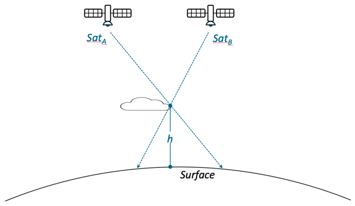
Figure 1. Displacement (difference in the apparent position) over the Earth surface of a tracer/AMV observed with different angles by two different satellites, SatA and SatB. This displacement is related to the tracer/AMV height, h, over the surface.
Remotesensing 18 02940 g001
Figure 2. Satellite A and Satellite B pairings (mandatory matches as solid lines; optional matches as dashed lines).
Remotesensing 18 02940 g002
Figure 3. Stereo implementation into HRW algorithm. Optional elements marked with an asterisk.
Remotesensing 18 02940 g003
Figure 4. Row (left) and column (right) static Look-Up Tables used to remap GOES-East/ABI imagery into the native MTG-I/FCI viewing geometry.
Remotesensing 18 02940 g004
Figure 5. Example of native GOES-East/ABI imagery (left) and once remapped with the defined Look-Up Tables into the native MTG-I/FCI viewing geometry (right), for 14 February 2025 at 1200 UTC. Radiance units for Channel 13 are mW m−2 sr−1 cm.
Remotesensing 18 02940 g005
Figure 6. Input and remapped Time Look-Up Tables for GOES-R/ABI, in seconds.
Remotesensing 18 02940 g006
Figure 7. East–West and North–South parallax Look-Up Tables, in pixels per km of height.
Remotesensing 18 02940 g007
Figure 8. Geoid and terrain height Look-Up Tables, in m.
Remotesensing 18 02940 g008
Figure 9. Sensitivity analysis of HRW stereo height assignment method for several values of the RMS residual threshold (in the lower scale) against ECMWF model analysis winds. The BIAS (in m/s, in light blue), the RMS (in m/s, in dark blue) and the percentage of AMVs with respect to the default configuration where RMS residuals < 0.25 pixels (in black) are shown.
Remotesensing 18 02940 g009
Figure 10. Direct comparison of assigned heights for 28 March 2025 15:30Z in the tropics for IR10.5 HRW AMVs.
Remotesensing 18 02940 g010
Figure 11. Low-level stereo and non-stereo HRW AMVs compared with LiDAR and ERA5 reanalysis. Zonal winds are indicated by the symbol “u” and meridional winds are indicated by the symbol “v” appearing in separate panels for stereo and non-stereo wind comparisons to ERA5. ERA5 Temperature, Relative Humidity (RH), and Cloud Coverage profiles provide additional context for meteorological conditions, showing where ERA5 has represented trackable cloud features and the presence of inversions that could challenge non-stereo height assignment methods relying on temperature versus height.
Remotesensing 18 02940 g011
Figure 12. Stereo and non-stereo AMVs, LiDAR and reanalysis comparison with vanishing lapse rate.
Remotesensing 18 02940 g012
Figure 13. High-level stereo and non-stereo AMVs, LiDAR and reanalysis with a large non-stereo AMV height assignment error.
Remotesensing 18 02940 g013
Figure 14. Comparison statistics between observed and reanalysis wind for stereo and non-stereo height assignments by case ordered chronologically.
Remotesensing 18 02940 g014
Figure 15. Distribution of stereo and non-stereo AMVs.
Remotesensing 18 02940 g015
Figure 16. Comparison between stereo and non-stereo height assignments for infrared AMVs.
Remotesensing 18 02940 g016
Figure 17. Comparison between ERA5 and HRW stereo and non-stereo infrared AMVs.
Remotesensing 18 02940 g017
Figure 18. Comparison between ERA5 and HRW stereo and non-stereo visible AMVs.
Remotesensing 18 02940 g018
Table 1. Daily statistics for stereo and non-stereo AMVs. High-level winds are those above 6 km, mid-level winds are between 2 km and 6 km, and low-level winds are below 2 km, using the stereo height assignment for the stratification.
ΔHeight (m)Stereo to ERA5 (m/s)Non-Stereo to ERA5 (m/s)
DateBandLevelCountMeanSigmaMAVDMVDRMSVDMAVDMVDRMSVD
03-Jan-2025IRHigh68,743116812654.13.83.97.47.47.6
17-Jan-2025IRHigh81,54810209784.34.04.08.08.08.1
31-Jan-2025IRHigh49,447128711414.54.24.28.78.68.6
14-Feb-2025IRHigh54,229135011534.13.83.88.89.29.3
28-Feb-2025IRHigh31,707115413223.83.53.57.57.67.7
14-Mar-2025IRHigh26,339112210414.44.24.27.27.27.2
28-Mar-2025IRHigh59,87092211334.34.04.07.16.96.9
03-Jan-2025IRMid19,7511436303.93.73.73.93.63.6
17-Jan-2025IRMid30,1303875563.12.92.94.24.04.0
31-Jan-2025IRMid17,342−1364823.73.43.53.13.03.0
14-Feb-2025IRMid46,7971345953.13.03.03.53.43.4
28-Feb-2025IRMid61,190976613.12.92.93.13.03.1
14-Mar-2025IRMid13,8462345973.43.33.33.94.04.0
28-Mar-2025IRMid53,9372285973.73.43.44.44.34.3
03-Jan-2025IRLow73,4661663263.63.33.34.23.93.9
17-Jan-2025IRLow63,9872404113.12.92.94.13.93.9
31-Jan-2025IRLow81,2701613262.92.72.73.22.92.9
14-Feb-2025IRLow134,6762273542.82.62.63.33.03.0
28-Feb-2025IRLow59,5571074723.73.53.54.24.14.1
14-Mar-2025IRLow42,2041413353.63.23.34.34.04.0
28-Mar-2025IRLow124,6271843953.33.13.14.13.93.9
03-Jan-2025VISHigh15258317063.73.53.55.75.85.9
17-Jan-2025VISHigh63156476573.83.43.46.76.56.5
31-Jan-2025VISHigh8649277754.23.93.98.78.58.6
14-Feb-2025VISHigh148510508953.53.23.27.57.67.7
28-Feb-2025VISHigh14234897613.22.82.85.35.15.2
14-Mar-2025VISHigh7958097263.43.13.14.95.15.1
28-Mar-2025VISHigh18107008173.93.63.66.26.06.0
03-Jan-2025VISMid28783664453.33.03.03.63.33.3
17-Jan-2025VISMid40284825002.92.72.73.93.73.7
31-Jan-2025VISMid10891884933.33.13.13.63.53.5
14-Feb-2025VISMid43603914682.72.52.53.73.53.5
28-Feb-2025VISMid65964384852.82.72.73.43.23.3
14-Mar-2025VISMid13655054962.72.52.54.34.24.3
28-Mar-2025VISMid57683585003.22.93.04.54.14.1
03-Jan-2025VISLow30,8192102712.82.52.63.83.53.5
17-Jan-2025VISLow22,3263113002.62.42.43.63.43.4
31-Jan-2025VISLow10,8343582052.52.32.32.92.82.8
14-Feb-2025VISLow35,8153102982.52.32.33.33.13.1
28-Feb-2025VISLow15,3323283153.22.92.94.34.14.1
14-Mar-2025VISLow24,6252212683.02.72.74.13.73.7
28-Mar-2025VISLow35,5512873042.92.62.74.13.73.7
Disclaimer/Publisher’s Note: The statements, opinions and data contained in all publications are solely those of the individual author(s) and contributor(s) and not of MDPI and/or the editor(s). MDPI and/or the editor(s) disclaim responsibility for any injury to people or property resulting from any ideas, methods, instructions or products referred to in the content.