Article

Complex-Valued HRU-Net with Cross-Gated Attention for PolSAR Semantic Segmentation

1
School of Physics and Electronic Information, Gannan Normal University, Ganzhou 341000, China
2
Jiangxi Province Key Laboratory of Multidimensional Intelligent Perception and Control, School of Information Engineering, Jiangxi University of Science and Technology, Ganzhou 341000, China
3
China Mobile Communications Group Jiangxi Co., Ltd. Ganzhou Branch, Ganzhou 341000, China
*
Author to whom correspondence should be addressed.
Remote Sens. 2026, 18(17), 2947; https://doi.org/10.3390/rs18172947
Submission received: 13 June 2026 / Revised: 8 August 2026 / Accepted: 20 August 2026 / Published: 2 September 2026
(This article belongs to the Section Engineering Remote Sensing)

Highlights

What are the main findings?
  • A lightweight complex-valued high-resolution U-Net (CV-HRU-Net) is proposed for polarimetric synthetic aperture radar (PolSAR) semantic segmentation. It maintains high-resolution complex-valued representations while progressively incorporating multi-resolution high-level semantic information during decoding.
  • A novel complex-valued cross-gated attention (CV-CGA) module uses encoder features to adaptively calibrate core decoder features through channel–spatial enhancement, Transformer-style cross-attention, and gated recalibration.
What are the implications of the main findings?
  • Experimental results demonstrate that the proposed CV-HRU-Net with CV-CGA jointly exploits phase-sensitive polarimetric information, high-resolution spatial details, and multi-resolution semantic information, thereby improving PolSAR land-cover segmentation accuracy and boundary delineation.
  • The performance gains achieved by CV-CGA indicate that encoder-guided calibration of core decoder features can improve semantic selectivity and boundary representation with only marginal model-size overhead.

Abstract

In recent years, U-Net-based architectures have been widely applied to polarimetric synthetic aperture radar (PolSAR) semantic segmentation. However, successive downsampling may lead to the loss of fine spatial details, while conventional U-Net-style decoder directly concatenates encoder features with the corresponding decoder features without explicitly accounting for their semantic discrepancy, potentially introducing redundant or irrelevant information and weakening feature discrimination. To address these limitations, this paper proposes a lightweight complex-valued high-resolution U-Net (CV-HRU-Net) with a complex-valued cross-gated attention (CV-CGA) module for PolSAR semantic segmentation. CV-HRU-Net employs a complex-valued high-resolution network (CV-HRNet) as the encoder to maintain high-resolution representations through parallel multi-resolution streams, while a complex-valued U-Net (CV-U-Net) decoder progressively incorporates multi-resolution high-level semantic features for pixel-wise prediction. To improve encoder–decoder feature interaction, CV-CGA adaptively calibrates the core decoder features using encoder information. Specifically, CV-CGA integrates the Convolutional Block Attention Module, Transformer-style cross-attention with decoder features as queries and encoder features as keys and values, and adaptive gated recalibration to enhance semantic selectivity and boundary representation. Experiments on two airborne and two spaceborne PolSAR datasets demonstrate that the proposed network achieves accurate land-cover segmentation and precise boundary delineation by jointly exploiting polarimetric phase relationships, fine spatial details, and multi-resolution semantic information. Furthermore, CV-CGA substantially improves segmentation accuracy and boundary F1 scores while introducing only marginal model-size overhead.

1. Introduction

Polarimetric synthetic aperture radar (PolSAR) provides all-weather and day-and-night active microwave imaging capabilities, enabling the acquisition of surface scattering information under complex observation conditions [1,2]. Effectively extracting discriminative information from PolSAR images for accurate land-cover semantic interpretation has long been an important research topic in this field [3,4,5,6]. As an important means of image interpretation, PolSAR semantic segmentation assigns a corresponding category to each image pixel, thereby transforming polarimetric observations into pixel-level land-cover interpretation results with explicit spatial distributions, regional structures, and boundary information. Therefore, it has important applications in agricultural monitoring, forest resource assessment, urban land-use mapping, environmental monitoring, and disaster management.
In recent years, substantial advances have been made in deep learning-based PolSAR semantic segmentation. According to the network architectures, existing methods can be broadly divided into CNN-based networks [7,8,9,10,11,12,13] and hybrid architectures combining CNNs with Transformers or multilayer perceptrons (MLPs) [14,15,16]. Owing to their local receptive fields, weight sharing, and hierarchical feature extraction capabilities, CNNs can effectively characterize the local spatial structures, texture information, and multiscale contextual information of PolSAR images. Therefore, CNN-based models remain widely used in PolSAR semantic segmentation. As a representative CNN architecture, U-Net adopts an encoder–decoder structure and employs skip connections to integrate the spatial details retained by the encoder with the semantic information recovered by the decoder, thereby providing an effective pixel-wise prediction [17]. However, the original U-Net was developed for medical image segmentation, and its direct application to PolSAR imagery is challenging because of substantial differences in imaging mechanisms and data characteristics between medical and polarimetric SAR images.
To adapt U-Net to PolSAR imagery, various architectural improvements have been proposed, including lightweight network structure [18], multiscale feature extraction [19], residual attention enhancement [20], and graph-based structural modeling [21,22]. Despite these improvements, these U-Net variants generally retain the hierarchical encoder–decoder paradigm, in which feature resolution is progressively reduced during encoding and subsequently recovered during decoding. Successive downsampling enlarges the receptive field and facilitates high-level semantic representation, but progressively decreases spatial resolution, making small-scale structures and boundary information susceptible to degradation. Moreover, encoder and decoder features differ in semantic level and information distribution, and their direct fusion may introduce redundant or irrelevant responses. For PolSAR images, shallow features are additionally susceptible to speckle noise and local scattering fluctuations, which may be propagated to the decoder through skip connections.
Beyond architectural improvements for feature extraction and information modeling, fully exploiting the complex-valued (CV) scattering information inherent in PolSAR data is another important means of improving semantic segmentation performance. Building on the theoretical foundations and basic computational framework for deep CV networks established by Trabelsi et al. [23], CV operations have been introduced into architectures such as U-Net and BiSeNet, enabling magnitude and phase information to be jointly modeled in the complex domain while preserving their intrinsic coupling [18,24,25]. Although these methods improve the utilization of CV polarimetric information, most are developed by extending conventional RV networks to the complex domain and have yet to adequately coordinate CV information modeling, high-resolution spatial representation, and multilevel semantic fusion. Moreover, the specific role of phase-sensitive polarimetric information in feature learning and its contribution to segmentation performance have not yet been systematically and intuitively analyzed.
To address the above issues, we propose a lightweight CV high-resolution U-Net (CV-HRU-Net) with a CV cross-gated attention (CV-CGA) module for PolSAR semantic segmentation, building upon the CV U-Net architecture. Specifically, a lightweight CV high-resolution encoder (CV-HRNet) is constructed based on the high-resolution network (HRNet) [26]. It continuously maintains high-resolution CV representations through parallel multiresolution branches and repeatedly exchanges information across different resolutions, thereby preserving fine spatial structures while capturing multiscale contextual features. Subsequently, a CV-U-Net decoder progressively fuses the multiresolution high-level semantic features produced by the encoder and gradually recovers spatial resolution, ultimately generating pixel-level land-cover segmentation results. To further improve information interaction between the encoder and decoder, CV-CGA is introduced to use encoder features as auxiliary information for adaptively calibrating the core decoder features. This design alleviates the semantic discrepancy between the two feature streams while suppressing redundant information and noise interference, thereby enhancing the semantic selectivity and boundary representation capability of the decoder features.
The main contributions of this study are summarized as follows:
(1)
A lightweight CV-HRU-Net is proposed, which integrates a CV high-resolution encoder and a CV-U-Net decoder within a unified end-to-end framework. Through parallel multiresolution branches, the network continuously maintains high-resolution CV representations and progressively fuses spatial details and high-level semantic information from different resolution branches during decoding, thereby facilitating the coordinated exploitation of polarimetric phase relationships, fine spatial structures, and multiscale semantic context.
(2)
A novel CV-CGA module is proposed to alleviate the semantic discrepancy between encoder and decoder features. The module integrates Convolutional Block Attention Module (CBAM)-based feature enhancement, Transformer-style cross-attention, and adaptive gated recalibration. It uses encoder features as auxiliary information to selectively calibrate the core decoder features, thereby suppressing redundant information and noise interference while enhancing their semantic selectivity and boundary representation capability.
(3)
Experiments are conducted on two airborne and two spaceborne PolSAR datasets. The experimental results demonstrate that the proposed network achieves highly accurate land-cover segmentation and performs particularly well in delineating complex boundaries. Further phase-randomization experiments verify the important contribution of polarimetric phase information to feature learning and semantic segmentation performance.

2. Related Work

2.1. U-Net-Based PolSAR Semantic Segmentation

U-Net extracts increasingly semantic features through its encoder and restores spatial resolution through its decoder, while skip connections fuse features from different levels. It has therefore been increasingly applied to PolSAR semantic segmentation. Early studies mainly focused on adapting this general encoder–decoder framework to PolSAR data. On the one hand, to address the limited availability of labeled PolSAR samples, transfer learning was introduced into fully convolutional segmentation networks such as U-Net to improve model training and generalization under limited training data [27]. On the other hand, different polarimetric representations, including coherency-matrix and polarimetric decomposition features, were employed as U-Net inputs to better exploit polarimetric scattering information represented in different forms [28].
Subsequent studies shifted toward architectural improvements to U-Net. Lightweight encoders and decoders combined with capsule-based feature modeling were introduced to enhance deep feature representation [18]. Multiscale residual learning and efficient convolutions were incorporated to improve feature extraction for land-cover objects at different scales [19], while CV residual attention was further employed to enhance multiresolution discriminative feature representation in PolSAR images [20]. More recently, the encoder–decoder paradigm of U-Net has been extended to the graph domain, where graph convolution, hierarchical graph representations, and cross-level or multiscale feature interactions have been introduced to improve the modeling of spatial neighborhoods and polarimetric relationships [21,22].
Overall, U-Net-based methods have made considerable progress in PolSAR image semantic segmentation. Nevertheless, effectively coordinating fine spatial representations, multiscale semantic information, and cross-level feature interactions remains an important research issue.

2.2. Attention-Based Feature Enhancement and Fusion for PolSAR Semantic Segmentation

Attention mechanisms have been widely applied to PolSAR semantic segmentation to suppress redundant and noise-induced responses, enhance discriminative features, and facilitate the effective fusion of information from different levels or sources. According to their information-modeling strategies, existing methods can be broadly categorized into three groups: convolutional feature recalibration, self-attention and Transformer-based modeling, and cross-attention and adaptive fusion.
In convolutional feature recalibration, channel attention, spatial attention, or their combination is commonly employed to adaptively adjust feature responses across different dimensions, such as polarimetric channels, feature channels, scale branches, and spatial locations, thereby emphasizing discriminative features while suppressing irrelevant information [9,29,30]. In self-attention and Transformer-based modeling, self-attention establishes long-range dependencies within the same feature stream and aggregates semantically related features from different spatial locations, thereby enhancing global contextual modeling and regional consistency [8]; Transformer architectures built upon multi-head self-attention can further capture semantic relationships across regions, scales, or feature levels [14,21]. In cross-attention and adaptive fusion, some methods establish correspondences between features from different sources to enable selective interactions among cross-level graph features, different polarimetric branches, and local and global information [21,31]; other methods further integrate scattering-distribution awareness, Transformer-based modeling, and boundary refinement to promote the coordinated representation of semantic information and spatial structures [15].
From the perspective of where attention modules are placed within the network, existing methods can be further grouped into four categories. The first places attention modules at the input stage or in the shallow layers of the encoder, mainly to select polarimetric features, regulate channel responses, and suppress redundant information [30]. The second incorporates them within the encoder or at the bottleneck, where channel attention, multiscale attention, self-attention, or Transformer architectures are employed to enhance feature representation, contextual modeling and high-level semantic representations [8,9,14,29,32]. The third deploys them in parallel branches, cross-level pathways, or encoder–decoder skip connections to establish relationships among features from different sources, scales, or semantic levels [21,31]. The fourth introduces them into the decoder, multiscale fusion head, or immediately before prediction to aggregate multiresolution features, recover spatial details, and strengthen the representation of land-cover boundaries and uncertain regions [15,31].
Overall, existing attention-based methods have effectively enhanced the feature extraction, information interaction, and multiscale fusion capabilities of PolSAR imagery. This study further investigates the interaction and fusion between encoder and decoder features within the U-Net architecture to alleviate their semantic discrepancy, reduce feature redundancy and noise interference, and thereby improve PolSAR semantic segmentation performance.

2.3. Utilization of CV Polarimetric Information in PolSAR Image Interpretation

Effectively exploiting the rich polarimetric information contained in PolSAR data is a fundamental issue in PolSAR image interpretation. Li and Chen proposed a generalized polarimetric correlation pattern to jointly characterize scattering correlations across multiple dimensions, including polarization, frequency, and space. They demonstrated the potential value of multidomain polarimetric correlation information for fine-grained target interpretation [33]. PolSAR observations are inherently CV, and each CV element can be equivalently represented in Cartesian and polar forms as z = x + i y = A e i ϕ , where x and y denote the real and imaginary components, respectively, while A and ϕ denote the magnitude and phase, respectively. The magnitude reflects the backscattering intensity of a target, whereas the relative phase and complex correlations among different polarimetric components contain complementary information related to target structure, orientation, and scattering mechanisms. From a deep learning perspective, existing approaches to exploiting CV PolSAR information can be broadly categorized into three categories.
The first category converts CV PolSAR data, such as the T matrix, into multichannel real-valued (RV) representations by separating magnitude, phase, real, and imaginary components or using polarimetric descriptors derived from scattering or coherency matrices. Zhang et al. separately modeled magnitude and phase information and fused them at multiple levels [34], while Jing et al. proposed PSRN to reconstruct spatial and relational information among polarimetric components [8]. These approaches can directly leverage mature RV network architectures and optimization techniques. However, decomposing CV data into separate RV channels does not explicitly preserve the intrinsic coupling between real and imaginary components or between magnitude and phase. Related comparisons further indicate that both input representation and computational domain affect the exploitation of polarimetric information [32,35].
The second category directly processes PolSAR data using CV networks to preserve the intrinsic coupling between real and imaginary components while jointly modeling magnitude, phase, and interchannel complex correlations. Representative studies include CV FCNs for pixel-level classification [36], lightweight CV DeepLabv3+ (L-CV-DeepLabv3+) [37] and CV U-Net with capsule embedding (CV-Cap-U-Net) [18], CV segmentation networks with Lovász–Softmax optimization [25], CV BiSeNetV2 with lightweight attention [24], lightweight CV Siamese networks with contrastive learning [38], CV convolutional Kolmogorov–Arnold networks [39], and three-dimensional CV networks for multiscale polarimetric–spatial feature extraction [40]. These methods preserve complex relationships more explicitly during feature transformation. However, many of them are developed by extending established RV backbones to the complex domain, while largely retaining their original network structures and feature-fusion strategies.
The third category adopts joint RV–CV dual-domain modeling, where the RV branch captures polarimetric power, statistical characteristics, and physically interpretable descriptors, while the CV branch preserves magnitude–phase coupling and interchannel complex correlations. Cross-domain fusion is then used to exploit their complementarity. Ma et al. jointly modeled physically meaningful RV polarimetric features and CV information containing relative phase and interchannel correlations within a dual-domain network [41]. Alkhatib et al. further integrated RV polarimetric descriptors derived from the coherency matrix with the original CV coherency information through cross-domain feature fusion [42]. Although this strategy integrates the interpretability of RV features with the information-preserving capability of CV representations, it may increase architectural and cross-domain fusion complexity.
Overall, RV networks offer mature computational frameworks but may weaken the intrinsic coupling of CV components, whereas CV networks preserve magnitude–phase relationships and interchannel complex correlations more explicitly. Joint RV–CV networks exploit the complementarity of both representations but introduce additional fusion complexity. In this work, we focus on CV representation learning for PolSAR semantic segmentation to exploit discriminative polarimetric information.

3. Method

3.1. Overall Architecture

The proposed lightweight CV-HRU-Net with CV-CGA is illustrated in Figure 1. It adopts an encoder–decoder framework, in which feature extraction and fusion are performed in the complex domain. Both the encoder and decoder are designed to be lightweight to reduce the risk of overfitting on relatively small PolSAR datasets [4,18,37]. The encoder employs CV-HRNet, which uses parallel multi-resolution branches and cross-resolution feature interaction to extract multi-scale information while maintaining high-resolution CV representations, thereby alleviating the loss of spatial details caused by successive downsampling. The decoder adopts a lightweight U-Net-style progressive reconstruction structure. It first aggregates deep semantic features from multi-resolution branches of the encoder and then continuously propagates the deep semantic information during progressive upsampling while successively incorporating intermediate- and shallow-level encoder features. In this manner, semantic information at different levels and high-resolution spatial details are progressively integrated into the decoder representations, enabling refined reconstruction of land-cover regions and their boundaries. Furthermore, a CV-CGA module is introduced into the feature interaction between the encoder and decoder. It uses encoder features at the corresponding resolution to adaptively calibrate the core decoder features, thereby enhancing their semantic selectivity and suppressing redundant or irrelevant information. Finally, the segmentation head maps the decoder features to produce pixel-wise land-cover segmentation results.

3.2. Complex-Valued Encoder

Inspired by the parallel multi-resolution representation strategy of HRNet, we construct a lightweight CV-HRNet as the encoder to extract multi-resolution CV features from PolSAR images. The encoder consists of three stages, each comprising a feature extraction module and a transition module. The feature extraction modules perform feature extraction within each branch while maintaining its spatial resolution. The transition modules are responsible for scale transformation between adjacent stages and, as required by the network architecture, perform cross-resolution feature interaction and construct new low-resolution branches, as illustrated in Figure 1.
The feature extraction module of the first stage consists of two CV convolution and activation blocks with 3 × 3 kernels and a stride of 1. These blocks perform preliminary feature extraction without changing the input spatial resolution and replace the computationally expensive residual blocks used in the original HRNet. In the transition module of the first stage, the original-resolution branch is retained, while a CV convolution with a stride of 2 is used to generate a branch at 1/2 of the input resolution.
The feature extraction module of the second stage contains two parallel branches, each comprising two 3 × 3 CV convolution and activation blocks. The two branches perform feature extraction at the original input resolution and 1/2 of the input resolution, respectively. In the transition module of the second stage, the two branches are spatially aligned and interact through 2× upsampling and CV convolutional downsampling with a stride of 2. Meanwhile, the lowest-resolution branch is further downsampled to generate a branch at 1/4 of the input resolution.
The feature extraction module of the third stage contains three parallel branches, each comprising three 3 × 3 CV convolution and activation blocks. The three branches perform feature extraction while maintaining the original input resolution, 1/2 of the input resolution, and 1/4 of the input resolution, respectively. In the transition module of the third stage, the three branches are spatially aligned and interact across resolutions through 2× and 4× upsampling, CV convolutional downsampling with a stride of 2, and two successive CV convolutional downsampling operations with a stride of 2. In addition, the lowest-resolution branch is further downsampled to generate a deep feature at 1/8 of the input resolution.
The principal operations in the CV encoder include CV convolution, ReLU activation, and integer-factor nearest-neighbor upsampling. CV convolutions with a stride of 1 are used to extract features while maintaining spatial resolution, whereas those with a stride of 2 are used to reduce feature resolution and construct new low-resolution branches.
Denote the input CV feature as X , and the CV convolution kernel as W . Then the output of the CV convolution is expressed as,
Y = X W = X W X W + i X W + W X
where denotes the convolution operation, and and denote the real and imaginary components, respectively.
For a CV feature X , the CV ReLU activation is defined as,
CReLU X = ReLU X + i ReLU X
where ReLU denotes the RV ReLU activation function.
During cross-resolution feature interaction, nearest-neighbor interpolation is employed to perform 2× or 4× upsampling of CV features. Let s be the upsampling factor, where s 2 , 4 . For a CV feature X , the upsampled feature can then be expressed as,
U s X = X 1 s
where U denotes the upsampling operation, denotes the channel-wise Kronecker product, and 1 s s × s is an all-ones matrix.

3.3. Complex-Valued Cross-Gated Attention Module

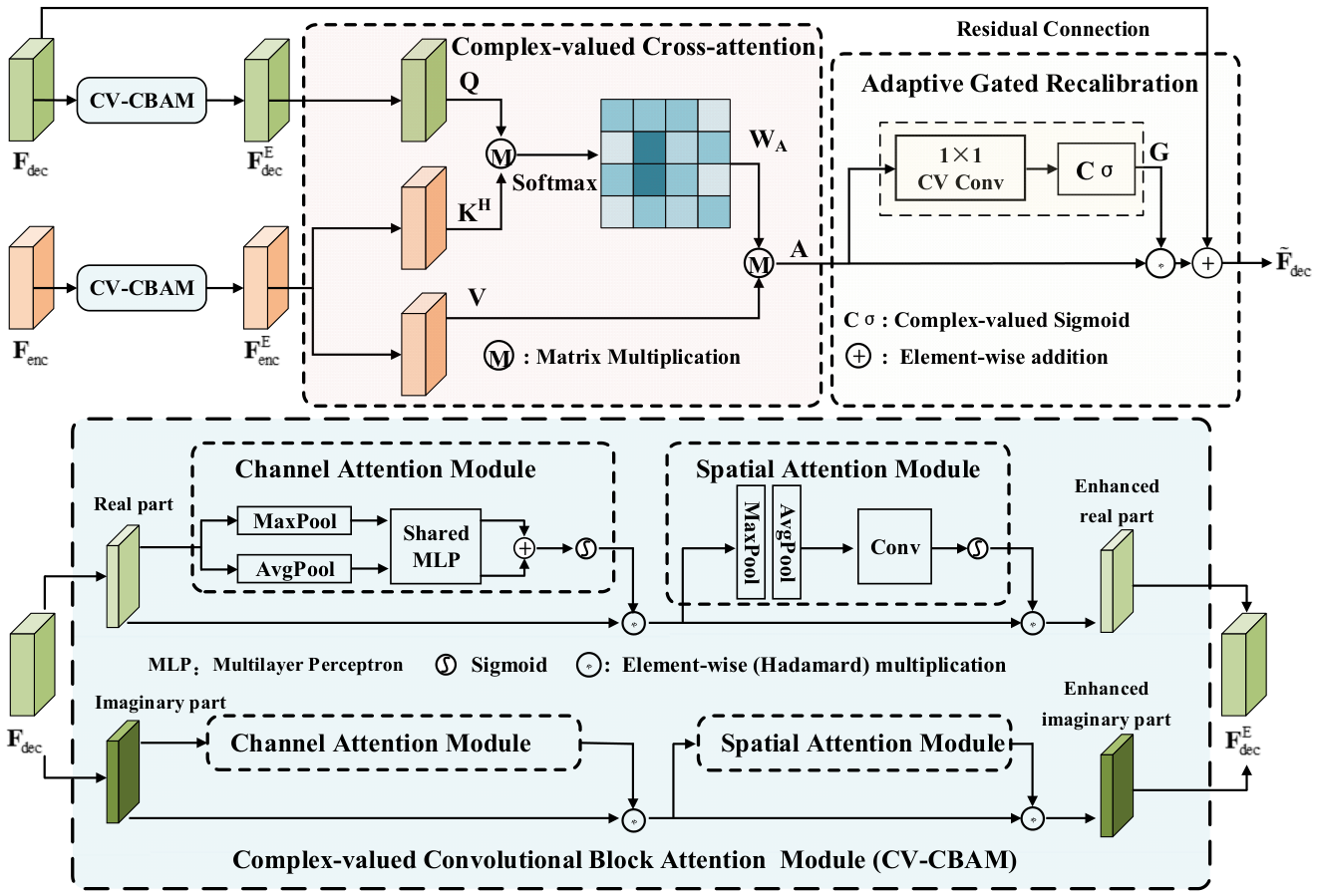
The CV-CGA module aims to adaptively calibrate the core decoder features using encoder features, thereby enhancing the semantic selectivity of the decoder representations while suppressing redundant or irrelevant responses. Features extracted at different depths of the encoder exhibit distinct representational characteristics. Shallow features retain abundant local textures and spatial details but have relatively limited semantic abstraction capability, whereas deep features contain stronger category-level semantic information but may lose some fine-grained spatial information during successive feature transformations. In comparison, intermediate encoder features provide a better balance between local structural representation and high-level semantic expression. Therefore, the intermediate features from the second encoder stage are selected to calibrate the core decoder features adaptively. As illustrated in Figure 2, CV-CGA consists of three main stages: CV channel–spatial attention enhancement, CV cross-attention, and adaptive gated recalibration.
Complex-Valued Channel–Spatial Attention Enhancement: The RV-CBAM [43] is extended to the complex domain to construct CV-CBAM, which enhances important channel and spatial responses in the encoder and decoder features, respectively, as illustrated in Figure 2. Both the channel-attention and spatial-attention components of conventional CBAM involve max-pooling operations. However, complex numbers do not possess a natural total ordering on the complex plane, and CV max-pooling therefore lacks a unique and generally accepted definition. To address this issue, the RV-CBAM is separately applied to the real and imaginary components of each CV feature, after which the two enhanced components are recombined into a CV representation.
Let the CV encoder features be F e n c , then the enhanced encoder feature obtained using CV-CBAM is expressed as,
F e n c E = CBAM F e n c + i CBAM F e n c
where CBAM denotes the RV channel- and spatial-attention enhancement performed by the RV-CBAM.
Similarly, for the CV decoder features F d e c , the enhanced decoder feature F d e c E is obtained in the same manner. This process emphasizes informative responses in both the encoder and decoder features along the channel and spatial dimensions.
Complex-Valued Cross-Attention: The enhanced decoder feature is used as the query ( Q ), whereas the enhanced encoder feature is used as the key ( K ) and value ( V ) for CV cross-attention. In this manner, the decoder feature can adaptively retrieve complementary information from the encoder feature according to its current semantic state. The query, key, and value are respectively expressed as,
Q = F d e c E W Q , K = F e n c E W K , V = F e n c E W V
where W Q , W K , and W V are trainable CV projection weights.
Then the Hermitian inner product between the query and key is calculated, and its real part is used as the similarity measure between the CV features. The attention-weight matrix W A and cross-attention output A are respectively given by
W A = Softmax Q K H d , A = W A V
where the superscript H denotes the Hermitian transpose, and d denotes the projected feature dimension of the query and key.
For an individual CV query element q and key element k , the real part of their Hermitian inner product can be written as
q k = q k cos ϕ q ϕ k
where ϕ q and ϕ k denote the phases of q and k , respectively.
Equation (7) describes the contribution of an individual feature dimension to the correlation score. When the query and key exhibit strong magnitude responses and a small phase difference in the corresponding feature dimension, that dimension produces a relatively large positive correlation contribution. In contrast, a response with a larger phase difference contributes a lower correlation score. The complete attention score is obtained by accumulating the correlation contributions over all feature dimensions. Therefore, the proposed CV cross-attention jointly exploits magnitude responses and relative phase relationships to establish content-dependent correlations between the encoder and decoder features.
Adaptive Gated Recalibration: Although cross-attention can retrieve complementary information from the encoder features, its output may still contain responses that are weakly related to the current decoding task. Therefore, a local CV adaptive gating mechanism is further introduced to selectively modulate the cross-attention output, suppress irrelevant responses, and enhance useful complementary information.
First, a 1 × 1 CV convolution is applied to the cross-attention output for channel mapping, after which a CV Sigmoid function is used to generate the gating weights,
G = C σ W g A
where W g denotes the weights of the 1 × 1 CV convolution, and C σ denotes the CV Sigmoid function. The CV Sigmoid function is defined as,
C σ = σ + i σ
where σ denotes the RV Sigmoid function.
Then the CV gating weights are used to modulate the cross-attention output element-wise. The modulated result is injected into the original core decoder feature as a residual calibration term, producing the calibrated decoder feature:
F ˜ d e c = F d e c + G A
where denotes CV Hadamard multiplication performed channel-wise and element-wise at each spatial location.
To further explain the effect of the CV gate, the gating weight and attention output are written in polar form as G = G e j ϕ G and A = A e j ϕ A , and their element-wise CV multiplication can then be expressed as,
G A = G A e i ϕ G + ϕ A
Equation (11) shows that the proposed gating mechanism jointly modulates the magnitude and phase of the attention features. On the one hand, the magnitude G of the gating weight adaptively attenuates or moderately enhances the attention responses. On the other hand, the phase ϕ G introduces an adaptive phase shift to the attention features. Because the CV Sigmoid function is independently applied to the real and imaginary components, both components of the gating weights lie within (0,1). Consequently, their magnitude and phase satisfy G 0 , 2 and ϕ G 0 , π 2 , respectively. It means that the resulting phase modulation corresponds to a constrained adaptive phase shift. Through this joint magnitude–phase modulation, CV-CGA not only controls the transmission strength of the cross-attention information but also adjusts its CV response relationships. The modulated complementary information is ultimately incorporated into the core decoder feature through a CV residual connection, enabling adaptive encoder-guided calibration of the decoder representation.
The procedure of CV-CGA is summarized in Algorithm 1.
Algorithm 1. CV-CGA Module
Input: Encoder feature F e n c ,
   Decoder feature F d e c
Output: Enhanced decoder feature F ˜ d e c
Stage 1: CV-CBAM Enhancement
  1. Decompose the encoder features into real and imaginary components:
            F e n c = F e n c + i F e n c
  2. Apply the RV-CBAM separately to the two components:
        F e n c E = CBAM F e n c , F e n c E = CBAM F e n c
  3. Recombine the enhanced components into the complex domain:
                 F e n c E = F e n c E + i F e n c E
  4. Apply Steps 1-3 to the decoder features F d e c :
             F d e c E = CBAM F d e c + i CBAM F d e c
Stage 2: Complex-Valued Cross-Attention
  5. Generate the query, key, and value:
             Q = F d e c E W Q , K = F e n c E W K , V = F e n c E W V
  6. Compute the attention-weights W A and the cross-attention output A :
             W A = Softmax Q K H d , A = W A V
Stage 3: Adaptive Gated Recalibration
  7. Generate the CV gating weights: G = C σ W g A
  8. Modulate the cross-attention output and perform residual calibration:
                 F ˜ d e c = F d e c + G A
Return:  F ˜ d e c

3.4. Complex-Valued Decoder

The decoder adopts a lightweight CV-U-Net to progressively fuse multi-resolution CV features and restore spatial resolution through three reconstruction stages, as shown in Figure 1. Unlike the original U-Net, each decoding stage receives two skip-connected features: the same-resolution feature from the corresponding encoder stage and the same-resolution aggregated feature generated after cross-resolution interaction at the end of the encoder. The former preserves stage-specific representations, while the latter provides complementary multi-resolution high-level semantic information. The three-stage decoding process is described as follows.
In the first decoding stage, the deep encoder feature at 1/8 of the input resolution is used as the initial core feature. It is first upsampled by a factor of 2 and then concatenated along the channel dimension with the two 1/4-resolution encoder features delivered through the skip connections. The concatenated features are subsequently fused through CV convolution to obtain the output of the first decoding stage.
In the second decoding stage, the output of the first stage is upsampled by a factor of 2 to obtain the core decoder feature at 1/2 of the input resolution. Because this stage lies between deep semantic propagation and high-resolution reconstruction, the CV-CGA module described in Section 3.3 is employed to adaptively calibrate the core decoder feature using the intermediate feature from the second encoder stage. The calibrated feature is then concatenated along the channel dimension with the two 1/2-resolution encoder features delivered through the skip connections. The resulting features are fused using CV convolution and activation blocks to produce the output of the second decoding stage.
In the third decoding stage, the output of the second stage is further upsampled by a factor of 2 to recover the original input resolution. It is then concatenated along the channel dimension with the two original-resolution encoder features delivered through the skip connections. CV convolution and activation blocks are subsequently applied to obtain the final high-resolution CV decoder feature.
To enable supervised learning with RV class labels, a CV segmentation head first maps the final decoder feature to C class channels, where C denotes the number of land-cover classes. Let F c denote the CV output corresponding to the c-th class, where c = 1, 2, …, C. Its magnitude is used as the RV class score, and the probability that each pixel belongs to class c is computed using the Softmax function,
P c = exp F c c = 1 C exp F c
where denotes the magnitude operation.
Finally, a RV cross-entropy loss is employed to supervise the discrepancy between the predicted class probabilities and the ground truth. The CV convolution, activation, and nearest-neighbor upsampling operations used in the decoder follow the definitions given in Section 3.2.

4. Experiments and Result Analysis

4.1. Datasets and Preprocessing

Two airborne and two spaceborne PolSAR datasets are used for the ablation and comparative experiments.
(1)
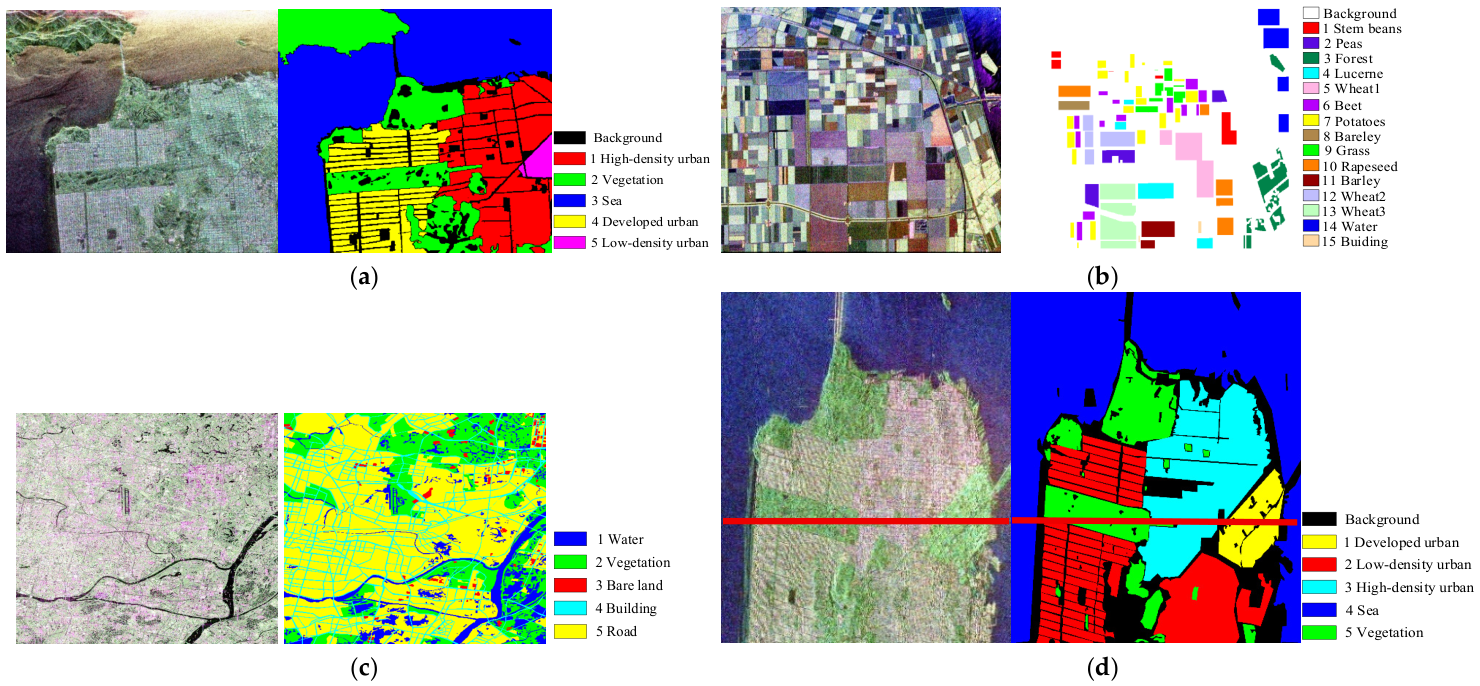
Airborne San Francisco Dataset [44]: The PolSAR data were acquired over the San Francisco Bay area in 1989 by the NASA/JPL Airborne Synthetic Aperture Radar (AIRSAR) system. The ground-truth map contains five annotated land-cover categories. The Pauli RGB image, corresponding ground-truth map, and class legend are shown in Figure 3a.
(2)
Airborne Flevoland dataset [45]: The PolSAR data were acquired over the agricultural region of Flevoland in 1989 by the AIRSAR system. The ground-truth map contains fifteen annotated land-cover categories. The Pauli RGB image, corresponding ground-truth map, and class legend are shown in Figure 3b.
(3)
Spaceborne AIR-PolSAR-Seg-2.0 dataset [46]: This dataset contains PolSAR data acquired by the Gaofen-3 satellite over four regions. In this study, the Guangzhou subset acquired in 2016 is used. Its ground-truth map contains five annotated land-cover categories. The Pauli RGB image, corresponding ground-truth map, and class legend are shown in Figure 3c.
(4)
Spaceborne San Francisco dataset [47]: The PolSAR data were acquired over the San Francisco Bay area in 2008 by the RADARSAT-2 satellite. The ground-truth map contains five annotated land-cover categories. The Pauli RGB image, corresponding ground-truth map, and class legend are shown in Figure 3d.
For data preprocessing, the airborne San Francisco and airborne Flevoland datasets are first mirror-padded along their boundaries so that both the image height and width are divisible by 64. The padded images are then cropped into non-overlapping 64 × 64 patches. To maintain spatial independence between the training and test sets as much as possible, these patches are partitioned according to their spatial locations, with 30% assigned to the training set and the remaining 70% assigned to the test set. For the Guangzhou subset of the spaceborne AIR-PolSAR-Seg-2.0 dataset, the publicly released data are provided as patches cropped with a 50% overlap ratio. In this study, these patches are further divided into training, validation, and test sets at a ratio of 7:2:1. For the spaceborne San Francisco dataset, a fixed spatial partition is adopted. As indicated by the red dividing line in Figure 3d, approximately 60% of the region above the line is assigned to the test set, whereas approximately 40% of the region below the line is assigned to the training set, thereby maintaining spatial independence between the training and test regions as much as possible. All training samples are augmented through rotation.
Under the monostatic reciprocity assumption, the 3 × 3 polarimetric coherency matrix T , derived from the fully polarimetric SAR scattering matrix, satisfies Hermitian symmetry. Therefore, only the six independent elements in its upper triangular part are required. The proposed CV network and the other CV networks used for comparison take these elements as input, i.e., T 11 , T 12 , T 13 , T 22 , T 23 , T 33 . The RV diagonal elements are represented as CV channels with zero imaginary components. To ensure that the RV comparison networks receive the same information content as their CV counterparts, the six independent coherency-matrix elements are decomposed into nine RV channels, expressed as T 11 , T 12 , T 13 , T 22 , T 23 , T 33 , T 12 , T 13 , T 23 .

4.2. Experimental Setup and Evaluation Metrics

All experiments are conducted in the following computing environment: Ubuntu 20.04.6 LTS, an Intel Xeon E5-2680 v4 CPU operating at 2.40 GHz (Intel, Santa Clara, CA, USA), an NVIDIA Tesla P100 PCIe GPU with 16 GB of memory (NVIDIA, Santa Clara, CA, USA), Keras 2.2, and Python 3.6. The network parameters are optimized using the Adam optimizer.
The intersection over union (IoU) is employed to evaluate the segmentation performance of each land-cover category. The mean intersection over union (mIoU), overall accuracy (OA), and mean pixel accuracy (MPA) are used to assess the overall segmentation performance [37]. In addition, the boundary F1 score (BF1) is adopted as a boundary-based metric to evaluate the ability of each model to delineate land-cover boundaries.
To define BF1, the boundary pixel sets are extracted from the predicted segmentation map and the corresponding ground-truth map using image-processing operations, and are denoted by B p and B g , respectively. For each predicted boundary pixel p B p , its Euclidean distance to the nearest ground-truth boundary pixel is defined as
d p = min g B g   d p , g
where g denotes a ground-truth boundary pixel and d , represents the Euclidean distance.
A predicted boundary pixel is considered correctly matched if its distance to the nearest ground-truth boundary pixel does not exceed a predefined tolerance threshold τ . Accordingly, the boundary precision is defined as,
P b = 1 B p p B p I d p τ
where B p denotes the number of predicted boundary pixels, I is the indicator function, and τ is set to 2 pixels.
Similarly, for each ground-truth boundary pixel g B g , its Euclidean distance to the nearest predicted boundary pixel is defined as
d g = min p B p   d g , p
The boundary recall, defined as the proportion of ground-truth boundary pixels correctly matched by the predicted boundaries, is expressed as
R b = 1 B g g B g I d g τ
where B g denotes the number of ground-truth boundary pixels.
BF1 is then calculated as the harmonic mean of the boundary precision and recall:
BF 1 = 2 P b R b P b + R b
A higher BF1 value indicates greater spatial consistency between the predicted and ground-truth boundaries, reflecting a stronger ability to recover land-cover contours and accurately delineate inter-class boundaries.

4.3. Ablation Experiments

Ablation Study on the Major Architectural Components: To evaluate the contributions of the high-resolution encoder, CV representation, and CGA module, a series of network variants are progressively constructed under a unified lightweight setting. First, a lightweight three-stage encoder–decoder U-Net with RV operations, denoted as RV-U-Net, is adopted as the baseline model. Its convolution, activation, upsampling, and other operations are then extended to the complex domain to construct CV-U-Net. Subsequently, the lightweight RV-HRNet and CV-HRNet designed according to Figure 1 are employed as high-resolution encoders and combined with the corresponding U-Net-style progressive decoders, forming RV-HRNet + RV-U-Net and CV-HRNet + CV-U-Net, respectively. RV-CGA is the RV counterpart of CV-CGA, as illustrated in Figure 2. The ablation results on the four datasets are presented in Table 1.
The results are analyzed following the progressive construction of the network variants. First, compared with RV-U-Net, RV-HRNet + RV-U-Net consistently achieves better overall performance across the four datasets. This demonstrates that parallel multi-resolution representations and cross-resolution feature interactions facilitate the extraction of multi-level semantic information while preserving fine spatial details. Second, replacing the RV architecture with its CV counterpart generally leads to further performance improvements, although minor fluctuations are observed in a few individual metrics. This indicates that CV operations can better preserve and exploit the intrinsic coupling between the real and imaginary components of PolSAR coherency matrices, thereby providing more informative feature representations. Third, incorporating RV-CGA into RV-HRNet + RV-U-Net improves most evaluation metrics across the four datasets, demonstrating the effectiveness of encoder-guided cross-attention and gated recalibration in the RV feature space. Nevertheless, BF1 decreases slightly on the spaceborne San Francisco dataset, suggesting that the boundary-enhancement effect of RV-CGA may vary with dataset characteristics. Finally, incorporating CV-CGA into CV-HRNet + CV-U-Net produces consistent improvements across all four datasets. The complete CV-HRNet + CV-U-Net + CV-CGA model achieves the best performance for every overall metric on all datasets. It also consistently outperforms the complete RV counterpart, confirming the complementarity of CV representation, the high-resolution architecture, CV representation, and CV-CGA-based feature calibration.
Ablation Study on the Internal Components of CV-CGA: Using the airborne San Francisco dataset as an example, a component-wise ablation study is conducted to evaluate the contributions of CV-CBAM, CV cross-attention, and adaptive gated recalibration within CV-CGA. CV-HRNet + CV-U-Net is adopted as the baseline model, and the results are presented in Table 2.
Compared with the baseline, CV-CBAM improves mIoU and BF1, while OA and MPA exhibit only minor changes. This suggests that CV-CBAM primarily strengthens local structural details and class-boundary representations through channel–spatial recalibration. CV cross-attention improves all four metrics, demonstrating that cross-level interactions between encoder and decoder features effectively exploit complementary semantic and spatial information.
Combining CV-CBAM with CV cross-attention further improves BF1, while mIoU, OA, and MPA change only marginally compared with using CV cross-attention alone. This indicates that CV-CBAM primarily complements cross-attention by refining local structures and boundary representations. Adding adaptive gated recalibration to CV cross-attention further improves both region segmentation and boundary delineation, confirming that the gating mechanism can adaptively regulate the injection of encoder information and reduce ineffective or excessive feature modulation.
When the three components are jointly employed, the complete model achieves the best performance across all four metrics. These results demonstrate that CV-CBAM enhances local structural and boundary information, CV cross-attention facilitates cross-level feature interaction, and adaptive gated recalibration controls the intensity of feature enhancement. Their complementary effects validate the effectiveness of the complete CV-CGA design on the airborne San Francisco dataset.
Ablation Study on the Insertion Position of CV-CGA: To investigate the influence of the insertion position, CV-CGA is individually applied to Stage 1, Stage 2, and Stage 3 of the decoder, as shown in Figure 1. A configuration in which CV-CGA is simultaneously applied to all three stages is also evaluated. The results on the airborne San Francisco dataset are presented in Table 3. Among the evaluated configurations, inserting CV-CGA only at Stage 2 achieves the best performance across all four metrics, indicating that the effectiveness of CV-CGA is closely related to the feature characteristics of the insertion stage.
Stage 1 is located in the deep, low-resolution portion of the decoder, where the features contain strong semantic information but substantially compressed spatial details. This limits the ability of CV-CGA to refine fine-grained structures and class boundaries. Stage 3 is close to the final prediction layer and preserves richer local textures and boundary details. However, its features are more susceptible to speckle noise and local fluctuations, while offering limited scope for further semantic refinement. By contrast, Stage 2 provides a more favorable balance between semantic abstraction and spatial resolution, enabling CV-CGA to effectively integrate encoder information and refine decoder features.
Applying CV-CGA to all three stages does not yield further improvements over the Stage 2 configuration. This may be because features at different decoder stages vary substantially in spatial resolution, semantic level, and response distribution. Repeated cross-attention and gated recalibration across multiple stages may therefore introduce redundant or inconsistent feature modulation. Overall, inserting CV-CGA only at Stage 2 provides the most effective configuration.

4.4. Comparative Experiments

Comparative experiments are conducted on four datasets. For the two airborne datasets, seven RV segmentation models are included for comparison: FCN [48], DeepLabv3+ [49], TransUNet [50], SegFormer [51], DSNet [52], CGRSeg [53], and VWFormer [54]. DSNet adopts a dual-branch same-resolution architecture, CGRSeg performs context-guided spatial feature reconstruction, and VWFormer employs a varying-window-attention-based multiscale decoder. Two CV models, L-CV-DeepLabv3+ [37] and CV-Cap-U-Net [18], are also included. For the two spaceborne datasets, two lightweight RV models, Fast-SCNN [55] and BiSeNetv2 [56], and two lightweight CV models, L-CV-DeepLabv3+ [37] and CV-Cap-U-Net [18], are selected for comparison.
Results on the Airborne San Francisco Dataset: Each model is independently trained ten times using different random seeds. Table 4 reports the mean and standard deviation of the test-set performance, where the class-wise results are measured using IoU. Among the seven RV models, TransUNet achieves the strongest overall performance, suggesting that global contextual modeling is beneficial for PolSAR land-cover segmentation. Among the existing CV models, L-CV-DeepLabv3+ achieves performance comparable to that of the best-performing RV models, whereas CV-Cap-U-Net provides clear improvements in mIoU, OA, and MPA. These results indicate that CV operations are beneficial for preserving and exploiting the coupled real and imaginary information in PolSAR data. However, the existing CV models do not achieve corresponding improvements in BF1, suggesting that CV representation alone does not guarantee superior boundary delineation.
The proposed method achieves the best performance across all four overall evaluation metrics and obtains the highest class-wise IoU for high-density urban, vegetation, developed urban, and low-density urban. Its advantage is particularly pronounced for the low-density urban class, for which several methods exhibit relatively low accuracy and large performance variations. For the sea class, the proposed method performs slightly below CV-Cap-U-Net, but the difference is small, and most methods already achieve high accuracy for this category. The proposed method also exhibits low standard deviations in the overall metrics, indicating stable performance across different random seeds. Overall, the proposed network achieves simultaneous improvements in region-level segmentation accuracy, class-balanced recognition, and boundary delineation.
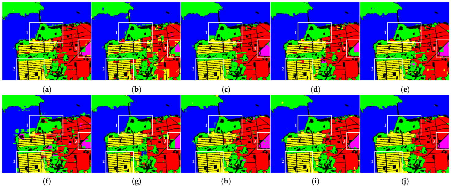
The full-scene segmentation results of all models are visualized in Figure 4. Three regions of interest, marked by white boxes 1–3, are selected for qualitative comparison with the ground truth shown in Figure 3a. Box 1 mainly contains sea, vegetation, and high-density urban areas. Several methods produce fragmented predictions or class confusion near the sea–vegetation and vegetation–high-density urban boundaries. In contrast, the proposed method preserves more coherent vegetation regions and produces clearer sea–land and vegetation–urban boundaries. Box 2 mainly contains developed urban areas and background. Some methods misclassify developed urban areas as high-density urban or produce incomplete regions, whereas the proposed method substantially reduces such confusion and better preserves the spatial integrity of the developed urban areas. Box 3 mainly contains low-density and high-density urban areas. Several methods misclassify parts of the low-density urban area as vegetation, while the proposed method more closely matches the ground truth and better preserves the boundary between the two urban categories. Overall, the proposed method reduces interclass confusion, improves regional completeness, and produces clearer class boundaries, consistent with its superior mIoU and BF1.
Results on the Airborne Flevoland dataset: Each model is independently trained ten times using different random seeds. Table 5 reports the mean and standard deviation of the test-set performance, with the class-wise results measured using IoU. Among the RV models, DSNet and VWFormer achieve relatively strong overall performance. Both existing CV models outperform the best-performing RV models across all four overall metrics, indicating that CV operations are more effective in preserving and exploiting the coupled real and imaginary information in PolSAR data. The proposed method achieves the highest mean values for mIoU, OA, MPA, and BF1. At the class level, it obtains the highest IoU for seven of the 15 land-cover categories and ranks among the top three methods for all categories, indicating balanced recognition performance across different land-cover types. It also exhibits relatively low standard deviations in the overall metrics, reflecting stable performance across different random seeds.
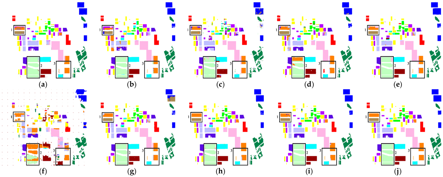
The full-scene segmentation results are shown in Figure 5. Three regions of interest, marked by black boxes 1–3, are selected for qualitative comparison with the ground truth in Figure 3b. In Boxes 1 and 2, several methods exhibit boundary deviations, incomplete predictions, or internal misclassifications, whereas the proposed method better preserves regional shapes and more closely matches the ground truth. Box 3 contains a small-scale land-cover region adjacent to two other classes. Several RV models partially misclassify or omit this region, while the existing CV models still show local boundary errors. In contrast, the proposed method recovers the small-scale region more completely and delineates adjacent class boundaries more accurately. Overall, these observations are consistent with its superior mIoU and BF1.
Results on the Guangzhou Subset of the Spaceborne AIR-PolSAR-Seg-2.0 Dataset: Each model is independently trained ten times using different random seeds. Table 6 reports the mean and standard deviation of the test-set performance, with the class-wise results measured using IoU. Among the two lightweight RV models, BiSeNetV2 achieves better overall performance than Fast-SCNN. L-CV-DeepLabv3+ yields slightly lower mIoU, OA, and MPA than BiSeNetV2 but achieves a higher BF1, indicating stronger boundary delineation. CV-Cap-U-Net further improves the region-level metrics, although its BF1 is slightly lower than that of L-CV-DeepLabv3+. The proposed method achieves the highest mean values for all four overall metrics and obtains the highest class-wise IoU for four of the five land-cover categories.
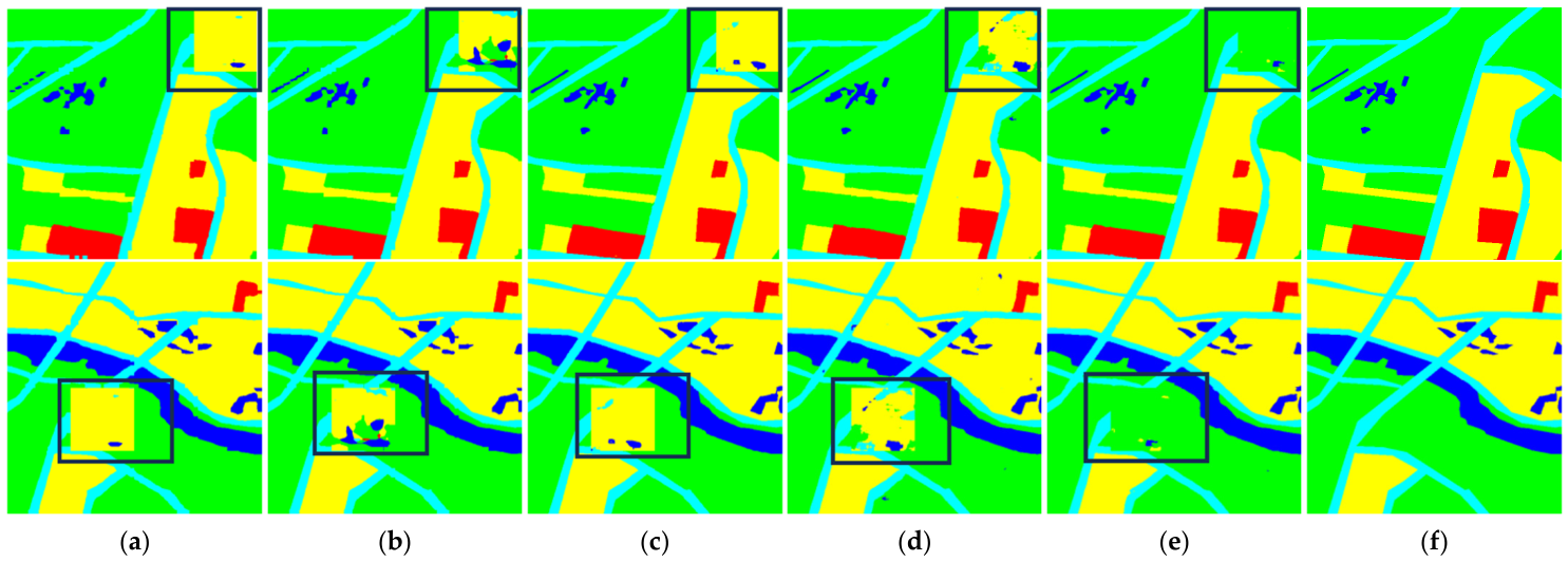
The segmentation results on two representative test patches are shown in Figure 6. Figure 6a–e present the results of the five lightweight models, while the corresponding ground truth is shown in Figure 6f. In the black-boxed regions, several methods exhibit local region fragmentation, spurious predictions, or interclass confusion. In contrast, the proposed method reduces these errors and better preserves the completeness of the land-cover regions. Although a few local misclassifications remain, its results more closely match the ground truth. These qualitative observations are consistent with its mIoU and BF1.
Results on the Spaceborne San Francisco Dataset: Each model is independently trained ten times using different random seeds. Table 7 reports the mean and standard deviation of the test-set performance, with the class-wise results measured using IoU. Among the two lightweight RV models, BiSeNetv2 achieves better overall performance than Fast-SCNN. It also outperforms L-CV-DeepLabv3+ across all four overall metrics. CV-Cap-U-Net further improves both region-level segmentation and boundary delineation. The proposed method achieves the highest values for mIoU, OA, MPA, and BF1 and obtains the highest class-wise IoU for four of the five land-cover categories.
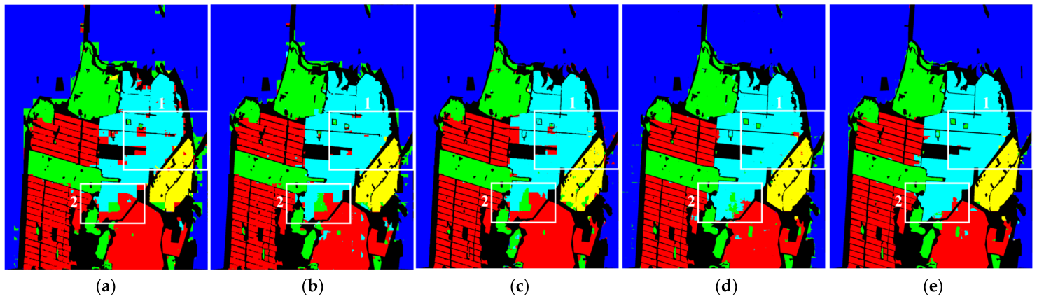
The full-scene segmentation results are shown in Figure 7. Two regions of interest, marked by white boxes 1 and 2, are selected for qualitative comparison with the ground truth shown in Figure 3d. In Box 1, several comparison methods confuse high-density urban areas with low-density urban areas to varying degrees, whereas the proposed method better distinguishes the two categories and delineates clearer class boundaries. In Box 2, some methods misclassify high-density urban areas as vegetation or low-density urban areas. In contrast, the proposed method substantially reduces such confusion and preserves a more complete high-density urban region, although a few local errors remain near the boundaries. Overall, the proposed method produces more coherent regions and clearer class boundaries, consistent with its leading mIoU and BF1.

5. Discussion

This section discusses the influence of phase perturbation on segmentation performance, visual analysis of the CV-CGA mechanism, and analysis of model complexity and performance. All analyses are conducted on the airborne San Francisco dataset.

5.1. Impact of Channel-Wise Phase Perturbation on Segmentation Performance

To investigate whether the proposed model exploits polarimetric phase relationships in addition to magnitude information, channel-wise phase perturbations are applied only to the CV polarimetric coherency matrices T in the test set, while the trained model parameters remain fixed. Specifically, for each pixel ( x , y ) , two independent channel-wise phase offsets, θ 1 x , y and θ 2 x , y , are randomly sampled, with the first polarimetric component used as the phase reference. A diagonal unitary matrix is then constructed as
U ( x , y ) = d i a g 1 , e i θ 1 x , y , e i θ 2 x , y
where θ 1 , θ 2 U δ , δ , δ 0 , π , and δ denotes the channel-wise phase-offset bound.
The perturbed coherency matrix is then obtained through the following unitary similarity transformation:
T ˜ ( x , y ) = U ( x , y ) T ( x , y ) U H ( x , y ) .
Because U ( x , y ) is unitary, this transformation preserves the diagonal elements and the magnitudes of the off-diagonal elements, while ensuring that T ˜ ( x , y ) remains Hermitian and positive semidefinite. The phases of the three perturbed off-diagonal elements after perturbation are given by
ϕ ˜ 12 = ϕ 12 θ 1 , ϕ ˜ 13 = ϕ 13 θ 2 , ϕ ˜ 23 = ϕ 23 + θ 1 θ 2 .
where ϕ 12 , ϕ 13 , and ϕ 23 are the original phases of T 12 , T 13 , and T 23 respectively. Thus, the phase changes in the three off-diagonal elements are physically consistent but mutually correlated rather than independently assigned. This perturbation scheme modifies the interchannel phase relationships while preserving the magnitudes and physical validity of the coherency matrix.
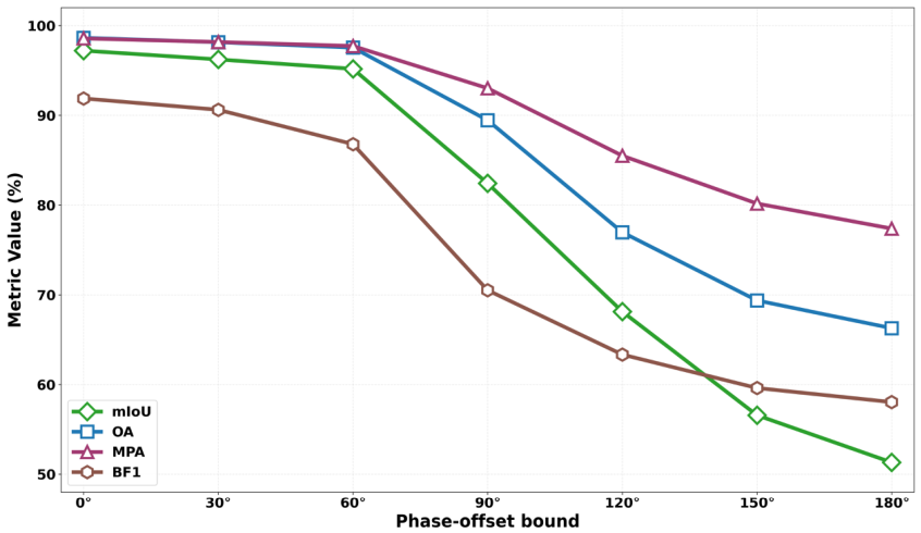
The channel-wise phase-offset bound δ is set to 0°, 30, 60°, 90°, 120°, 150°, and 180°. The corresponding test-set results are reported in Table 8, and the performance trends are shown in Figure 8. As δ increases, all four evaluation metrics decrease monotonically, indicating that the segmentation performance is sensitive to changes in polarimetric phase relationships. Within the range of 0–60°, mIoU, OA, and MPA decrease only slightly, whereas BF1 exhibits a more noticeable reduction, suggesting that boundary delineation is more sensitive to mild phase perturbations. When δ exceeds 60°, the performance deteriorates markedly, indicating that strong phase perturbations disrupt the original complex correlations among the polarimetric channels and weaken both class discrimination and boundary localization. At δ = 180 , mIoU and BF1 decrease from 97.21% and 91.88% to 51.32% and 58.04%, respectively. These results confirm that the proposed model effectively exploits polarimetric phase relationships rather than relying solely on magnitude information.

5.2. Visual Analysis of the CV-CGA Mechanism

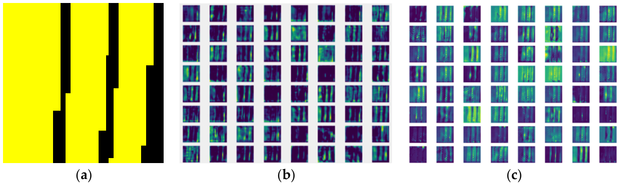
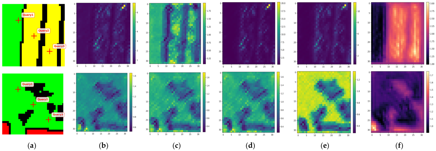
Visual Comparison of Decoder Features With and Without CV-CGA: To examine the influence of CV-CGA on decoder representations, the feature maps at decoder Stage 2, highlighted by the red dashed ellipse in Figure 1, are visualized before and after the introduction of CV-CGA. Figure 9a shows the ground truth of the input test sample, while Figure 9b and Figure 9c show the corresponding decoder features without and with CV-CGA, respectively. As shown in Figure 9a, the sample contains several elongated background regions with narrow and irregular boundaries. Without CV-CGA, some feature channels respond to these structures, but the activations are relatively scattered and spatially discontinuous. After introducing CV-CGA, the responses in multiple channels become more concentrated and continuous along the elongated background regions. In addition, some channels emphasize the interiors of these regions, whereas others respond more strongly to their boundaries, suggesting improved complementarity among the decoder features. These observations indicate that CV-CGA enhances the spatial selectivity of the decoder representations and suppresses scattered or irrelevant responses.
Visualization of Cross-Attention and Feature Recalibration: To further examine the working mechanism of CV-CGA, the cross-attention weights and the strength of encoder-guided feature correction are visualized. Assuming that both the encoder and decoder feature maps have a spatial size of 32 × 32, the encoder keys and decoder queries each contain 1024 spatial positions. The complete cross-attention matrix W A 1024 × 1024 describes the attention relationships between all decoder-query and encoder-key positions. Each row of W A corresponds to a decoder query, each column corresponds to an encoder key, and W A i , j denotes the attention weight assigned by the i-th (1 ≤ i ≤ 32) decoder position to the j-th (1 ≤ j ≤ 32) encoder position.
Since the complete attention matrix is too large for direct visualization, two complementary strategies are adopted. First, the i-th row of W A is reshaped into a 32 × 32 map to obtain a query-specific attention map, which shows the encoder positions from which a particular decoder location retrieves information. Second, all rows of W A are averaged and reshaped into a 32 × 32 map to obtain the global attention map, which reflects the overall contribution of different encoder positions to the decoder. In addition, the magnitude of the encoder-guided correction term in (11) is visualized as a correction-strength map, characterizing the spatial distribution of the residual feature updates after adaptive gated recalibration.
Figure 10a shows the ground-truth maps of two test samples, with three selected query locations marked by red crosses. The upper sample contains several continuous elongated background regions, whereas the lower sample contains irregular and relatively isolated background regions. Figure 10b presents the corresponding global attention maps, Figure 10c–e show the query-specific attention maps, and Figure 10f presents the correction-strength maps.
For both samples, the global attention maps exhibit clear spatial nonuniformity, indicating that the decoder assigns different levels of importance to different encoder positions rather than aggregating them uniformly. Although the three query-specific attention maps share some common spatial patterns, they also display distinct local responses. This suggests that different decoder positions adaptively retrieve contextual information from different encoder regions according to their semantic requirements. The correction-strength maps also exhibit spatially nonuniform responses. Relatively stronger feature updates tend to occur around structurally complex regions and class-transition areas, whereas broad homogeneous regions generally receive weaker corrections. Consequently, CV-CGA provides spatially selective feature correction and strengthens the representation of complex structures and class boundaries.

5.3. Analysis of Model Complexity and Performance

The model complexity, runtime efficiency, and segmentation accuracy of the RV- and CV-HRU-Net variants are reported in Table 9. The RV- and CV-HRU-Net share the same overall network topology, differing primarily in their numerical representations and corresponding RV or CV operations. Doubling the channel width of RV-HRU-Net substantially increases both the parameters and FLOPs but decreases mIoU, indicating that simply enlarging the capacity of the RV network does not necessarily improve PolSAR segmentation performance. Compared with the doubled-width RV-HRU-Net, CV-HRU-Net without CV-CGA achieves higher mIoU with fewer parameters, suggesting that CV modeling is more effective than merely increasing the capacity of the RV network. After CV-CGA is incorporated, the parameters and FLOPs increase by only approximately 1.0% and 1.4%, respectively, while mIoU improves by 3.62 percentage points. This demonstrates that CV-CGA provides a substantial performance gain with only marginal increases in model size and theoretical computational complexity. Nevertheless, the inference latency increases and the FPS decreases, mainly because CV cross-attention involves matrix multiplication, Softmax normalization, tensor rearrangement, and gated modulation. Overall, the proposed model achieves the highest segmentation accuracy among the evaluated variants while maintaining a compact parameter scale, demonstrating a favorable accuracy–model-size trade-off.

6. Conclusions

A lightweight CV-HRU-Net with CV-CGA is proposed for PolSAR semantic segmentation in this paper. The proposed network consists of a CV-HRNet encoder, a CV-CGA-enhanced skip connection, and a progressive CV-U-Net decoder. The encoder adopts parallel multi-resolution branches, while the decoder progressively integrates multi-resolution features. Embedded in the second skip connection, CV-CGA combines CV-CBAM, CV cross-attention, and adaptive gated recalibration. In addition to conventional region-based metrics, BF1 is introduced as a complementary measure of class-boundary quality. Experimental results on two airborne and two spaceborne PolSAR datasets demonstrate that the proposed network achieves superior overall segmentation performance and more accurate delineation of complex class boundaries by jointly exploiting polarimetric phase information, high-resolution spatial details, and multi-resolution high-level semantic information. Meanwhile, the proposed model maintains a compact parameter scale, and CV-CGA provides substantial performance improvements with only marginal increases in parameters. Future work will focus on incorporating explicit physical scattering mechanisms into the CV feature-learning process to improve the physical interpretability and discriminative capability of the learned representations. Domain adaptation will also be investigated to enhance the generalization ability of the network across different sensors, imaging conditions, spatial resolutions, and geographical regions. In addition, more efficient CV operations will be explored to reduce runtime costs while retaining the advantages of CV representation learning.

Author Contributions

Conceptualization, X.X.; methodology, X.X. and L.Y.; software, P.X., Y.G. and X.J.; investigation, P.X. and X.J.; formal analysis, P.X. and X.J.; validation, X.X., L.Y. and M.L.; resources, X.X.; data curation, L.Y. and M.L.; writing—original draft preparation, P.X. and X.X.; writing—review and editing, X.X., P.X., L.Y., M.L., Y.G. and X.J.; visualization, L.Y. and P.X.; supervision, X.X. and L.Y.; project administration, X.X. and L.Y.; funding acquisition, X.X., L.Y. and M.L. All authors have read and agreed to the published version of the manuscript.

Funding

This research was funded by the National Natural Science Foundation of China (no. 62561003, no. 62261027, no. 62566028, and no. 62266020), the Natural Science Foundation of Jiangxi Province (no. 20262BAC240426 and no. 20252BAC240198), and the Jiangxi Provincial Graduate Innovation Special Foundation under Grant YC2024-S571.

Data Availability Statement

The AIRSAR Flevoland dataset is available online at https://airsar.jpl.nasa.gov/, accessed on 1 June 2026. The AIRSAR San Francisco and RADARSAT-2 San Francisco datasets are available online at https://ietr-lab.univ-rennes1.fr/polsarpro-bio/, accessed on 1 June 2026. The Gaofen-3 AIR-PolSAR-Seg-2.0 dataset is available online at https://radars.ac.cn/web/data/getData?dataType=SARDataset, accessed on 1 June 2026. The source code for the proposed CV-HRU-Net method is available online at https://github.com/SmartSensingRadar/CV-HRUNet, accessed on 20 June 2026.

Acknowledgments

During the preparation of this manuscript, the authors used DeepSeek (V4-Flash version), Gemini (3.6 Flash version), and ChatGPT (5.6 version) for the purposes of preliminary language polishing and grammar correction. The authors have reviewed and edited the output and take full responsibility for the content of this publication.

Conflicts of Interest

Author Yuting Guo was employed by the company China Mobile Communications Group Jiangxi Co., Ltd. Ganzhou Branch. The remaining authors declare that the research was conducted in the absence of any commercial or financial relationships that could be construed as a potential conflict of interest.

References

  1. Zhang, Q.; He, C.; He, B.; Tong, M. Learning Scattering Similarity and Texture-Based Attention With Convolutional Neural Networks for PolSAR Image Classification. IEEE Trans. Geosci. Remote Sens. 2023, 61, 5207419. [Google Scholar] [CrossRef] [Scilit]
  2. Wang, S.; Guo, Y.; Hua, W.; Liu, X.; Song, G.; Hou, B.; Jiao, L. Semi-Supervised PolSAR Image Classification Based on Improved Tri-Training With a Minimum Spanning Tree. IEEE Trans. Geosci. Remote Sens. 2020, 58, 8583–8597. [Google Scholar] [CrossRef] [Scilit]
  3. Zhang, J.; Han, F.; Zhuang, D.; Zhang, L.; Zou, B.; Yuan, L. Toward Interpretable PolSAR Image Classification: Polarimetric Scattering Mechanism Informed Concept Bottleneck and Kolmogorov–Arnold Network. IEEE Trans. Geosci. Remote Sens. 2026, 64, 5200716. [Google Scholar] [CrossRef] [Scilit]
  4. Huang, J.; Liu, X. A Method for Land-Cover Classification of Fully Polarimetric SAR Images by Fusing LiteDSANet and Polarization Feature-Guided DenseCRF. Remote Sens. 2026, 18, 1631. [Google Scholar] [CrossRef] [Scilit]
  5. Ghanbari, M.; Xu, L.; Clausi, D.A. Local and Global Spatial Information for Land Cover Semisupervised Classification of Complex Polarimetric SAR Data. IEEE J. Sel. Top. Appl. Earth Obs. Remote Sens. 2023, 16, 3892–3904. [Google Scholar] [CrossRef] [Scilit]
  6. Liao, L.; Zhao, Q.; Song, W. Monitoring of Oil Spill Risk in Coastal Areas Based on Polarimetric SAR Satellite Images and Deep Learning Theory. Sustainability 2023, 15, 14504. [Google Scholar] [CrossRef] [Scilit]
  7. Ding, L.; Zheng, K.; Lin, D.; Chen, Y.; Liu, B.; Li, J.; Bruzzone, L. MP-ResNet: Multipath Residual Network for the Semantic Segmentation of High-Resolution PolSAR Images. IEEE Geosci. Remote Sens. Lett. 2022, 19, 4014205. [Google Scholar] [CrossRef] [Scilit]
  8. Jing, H.; Wang, Z.; Sun, X.; Xiao, D.; Fu, K. PSRN: Polarimetric Space Reconstruction Network for PolSAR Image Semantic Segmentation. IEEE J. Sel. Top. Appl. Earth Obs. Remote Sens. 2021, 14, 10716–10732. [Google Scholar] [CrossRef] [Scilit]
  9. Sun, J.; Yang, S.; Gao, X.; Ou, D.; Tian, Z.; Wu, J.; Wang, M. MASA-SegNet: A Semantic Segmentation Network for PolSAR Images. Remote Sens. 2023, 15, 3662. [Google Scholar] [CrossRef] [Scilit]
  10. Chu, B.; Chen, J.Y.; Chen, J.; Pei, X.Y.; Yang, W.; Gao, F.; Wang, S.C. SDCAFNet: A Deep Convolutional Neural Network for Land-Cover Semantic Segmentation With the Fusion of PolSAR and Optical Images. IEEE J. Sel. Top. Appl. Earth Obs. Remote Sens. 2022, 15, 8928–8942. [Google Scholar] [CrossRef] [Scilit]
  11. Zeng, X.; Wang, Z.R.; Sun, X.; Chang, Z.H.; Gao, X.; Zhao, L.J.; Kang, J. DENet: Double-Encoder Network With Feature Refinement and Region Adaption for Terrain Segmentation in PolSAR Images. IEEE Trans. Geosci. Remote Sens. 2022, 60, 5217419. [Google Scholar] [CrossRef] [Scilit]
  12. Xiao, D.; Wang, Z.; Wu, Y.; Gao, X.; Sun, X. Terrain Segmentation in Polarimetric SAR Images Using Dual-Attention Fusion Network. IEEE Geosci. Remote Sens. Lett. 2022, 19, 4006005. [Google Scholar] [CrossRef] [Scilit]
  13. Mohammadimanesh, F.; Salehi, B.; Mandianpari, M.; Gill, E.; Molinier, M. A new fully convolutional neural network for semantic segmentation of polarimetric SAR imagery in complex land cover ecosystem. ISPRS J. Photogramm. Remote Sens. 2019, 151, 223–236. [Google Scholar] [CrossRef] [Scilit]
  14. Liu, K.; Zheng, D.; Fan, J. Hybrid CNN-Transformer For Marine Aquaculture Semantic Segmentation Based on Polsar Images. In Proceedings of the 2024 IEEE International Geoscience and Remote Sensing Symposium (IGARSS), Athens, Greece, 7–12 July 2024; pp. 8255–8258. [Google Scholar] [CrossRef] [Scilit]
  15. Fang, X.; Chen, N.; Jiang, Y.; He, B.; He, C. A Hybrid Framework With Scattering Distribution Perception and Edge Refinement for PolSAR Image Segmentation. IEEE J. Sel. Top. Appl. Earth Obs. Remote Sens. 2025, 18, 29032–29049. [Google Scholar] [CrossRef] [Scilit]
  16. Wang, Z.; Wang, Z.; Qiu, X.; Zhang, Z. Global Polarimetric Synthetic Aperture Radar Image Segmentation with Data Augmentation and Hybrid Architecture Model. Remote Sens. 2024, 16, 380. [Google Scholar] [CrossRef] [Scilit]
  17. Ronneberger, O.; Fischer, P.; Brox, T. U-Net: Convolutional Networks for Biomedical Image Segmentation. In Medical Image Computing and Computer-Assisted Intervention—MICCAI 2015; Lecture Notes in Computer Science; Springer: Cham, Switzerland, 2015; Volume 9351, pp. 234–241. [Google Scholar] [CrossRef] [Scilit]
  18. Yu, L.; Shao, Q.; Guo, Y.; Xie, X.; Liang, M.; Hong, W. Complex-Valued U-Net with Capsule Embedded for Semantic Segmentation of PolSAR Image. Remote Sens. 2023, 15, 1371. [Google Scholar] [CrossRef] [Scilit]
  19. Xie, W.; Wang, R.N.; Yang, X.; Li, Y.H. Research on Multi-scale Residual UNet Fused with Depthwise Separable Convolution in PolSAR Terrain Classification. J. Electron. Inf. Technol. 2023, 45, 2975–2985. [Google Scholar] [CrossRef]
  20. Ren, S.; Zhou, F. PolSAR Image Classification with Complex-Valued Residual Attention Enhanced U-NET. In Proceedings of the 2021 IEEE International Geoscience and Remote Sensing Symposium (IGARSS), Brussels, Belgium, 11–16 July 2021; pp. 3045–3048. [Google Scholar] [CrossRef] [Scilit]
  21. Ren, S.; Zhou, F.; Bruzzone, L. Transfer-Aware Graph U-Net with Cross-Level Interactions for PolSAR Image Semantic Segmentation. Remote Sens. 2024, 16, 1428. [Google Scholar] [CrossRef] [Scilit]
  22. Song, W.; Liu, Q.; Pu, K.; Jiang, Y.; Wu, Y. Multiscale Attention-Enhanced Complex-Valued Graph U-Net for PolSAR Image Classification. Remote Sens. 2025, 17, 3943. [Google Scholar] [CrossRef] [Scilit]
  23. Trabelsi, C.; Bilaniuk, O.; Zhang, Y.; Serdyuk, D.; Subramanian, S.; Santos, J.F.; Mehri, S.; Rostamzadeh, N.; Bengio, Y.; Pal, C.J. Deep Complex Networks. In Proceedings of the International Conference on Learning Representations (ICLR 2018), Vancouver, BC, Canada, 30 April–3 May 2018. [Google Scholar]
  24. Xu, R.; Zhang, S.; Dong, C.; Mei, S.; Zhang, J.; Zhao, Q. Lightweight Attention Refined and Complex-Valued BiSeNetV2 for Semantic Segmentation of Polarimetric SAR Image. Remote Sens. 2025, 17, 3527. [Google Scholar] [CrossRef] [Scilit]
  25. Guo, R.; Zhao, X.; Guo, L.; Xu, R.; Liang, Y. A Complex-Valued PolSAR Image Segmentation Network With Lovász-Softmax Loss Optimization. IEEE J. Miniat. Air Space Syst. 2024, 5, 100–107. [Google Scholar] [CrossRef] [Scilit]
  26. Sun, K.; Xiao, B.; Liu, D.; Wang, J. Deep High-Resolution Representation Learning for Human Pose Estimation. In Proceedings of the 2019 IEEE/CVF Conference on Computer Vision and Pattern Recognition (CVPR), Long Beach, CA, USA, 16–20 June 2019; pp. 5686–5696. [Google Scholar] [CrossRef] [Scilit]
  27. Wu, W.; Li, H.; Li, X.; Guo, H.; Zhang, L. PolSAR Image Semantic Segmentation Based on Deep Transfer Learning—Realizing Smooth Classification With Small Training Sets. IEEE Geosci. Remote Sens. Lett. 2019, 16, 977–981. [Google Scholar] [CrossRef] [Scilit]
  28. Turkar, V.; Checker, J.; De, S.A.; Singh, G. Impact of G4U and 7-component target decomposition on PolSAR image semantic segmentation. Adv. Space Res. 2022, 70, 3798–3810. [Google Scholar] [CrossRef] [Scilit]
  29. Fang, Z.; Zhang, G.; Dai, Q.; Xue, B.; Wang, P. Hybrid Attention-Based Encoder–Decoder Fully Convolutional Network for PolSAR Image Classification. Remote Sens. 2023, 15, 526. [Google Scholar] [CrossRef] [Scilit]
  30. Zhou, X.Y.; Li, T.; Peng, D.L. PCA-Aware Attention Feature Fusion With Complex-Valued Adaptive Weighted UNet for PolSAR Classification. IEEE J. Sel. Top. Appl. Earth Obs. Remote Sens. 2026, 19, 7058–7083. [Google Scholar] [CrossRef] [Scilit]
  31. Chen, H.; Hou, Y.; Fang, X.; He, C. Enhanced PolSAR Image Segmentation with Polarization Channel Fusion and Diffusion-Based Probability Modeling. Electronics 2025, 14, 791. [Google Scholar] [CrossRef] [Scilit]
  32. Hochstuhl, S.; Pfeffer, N.; Thiele, A.; Hammer, H.; Hinz, S. Your Input Matters—Comparing Real-Valued PolSAR Data Representations for CNN-Based Segmentation. Remote Sens. 2023, 15, 5738. [Google Scholar] [CrossRef] [Scilit]
  33. Li, H.-L.; Chen, S.-W. General Polarimetric Correlation Pattern: A Visualization and Characterization Tool for Target Joint-Domain Scattering Mechanisms Investigation. IEEE Trans. Geosci. Remote Sens. 2026, 64, 5200417. [Google Scholar] [CrossRef] [Scilit]
  34. Zhang, L.M.; Dong, H.W.; Zou, B. Efficiently utilizing complex-valued PolSAR image data via a multi-task deep learning framework. ISPRS J. Photogramm. Remote Sens. 2019, 157, 59–72. [Google Scholar] [CrossRef] [Scilit]
  35. Barrachina, J.A.; Ren, C.; Morisseau, C.; Vieillard, G.; Ovarlez, J.-P. Comparison Between Equivalent Architectures of Complex-valued and Real-valued Neural Networks—Application on Polarimetric SAR Image Segmentation. J. Signal Process. Syst. 2023, 95, 57–66. [Google Scholar] [CrossRef] [Scilit]
  36. Cao, Y.; Wu, Y.; Zhang, P.; Liang, W.; Li, M. Pixel-Wise PolSAR Image Classification via a Novel Complex-Valued Deep Fully Convolutional Network. Remote Sens. 2019, 11, 2653. [Google Scholar] [CrossRef] [Scilit]
  37. Yu, L.; Zeng, Z.; Liu, A.; Xie, X.; Wang, H.; Xu, F.; Hong, W. A Lightweight Complex-Valued DeepLabv3+ for Semantic Segmentation of PolSAR Image. IEEE J. Sel. Top. Appl. Earth Obs. Remote Sens. 2022, 15, 930–943. [Google Scholar] [CrossRef] [Scilit]
  38. Jiang, Y.; Du, R.; Song, W.; Zhang, P.; Liu, L.; Zhang, Z. Lightweight Complex-Valued Siamese Network for Few-Shot PolSAR Image Classification. Remote Sens. 2026, 18, 344. [Google Scholar] [CrossRef] [Scilit]
  39. Kuang, Z.; Liu, S.; Bi, H.; He, L.; Li, F. CV-CPKAN: Complex-Valued Convolutional Kolmogorov–Arnold Framework for PolSAR Image Classification. Remote Sens. 2026, 18, 330. [Google Scholar] [CrossRef] [Scilit]
  40. Jiang, N.; Zhao, W.; Guo, J.; Zhao, Q.; Zhu, J. Multi-Scale Feature Extraction with 3D Complex-Valued Network for PolSAR Image Classification. Remote Sens. 2025, 17, 2663. [Google Scholar] [CrossRef] [Scilit]
  41. Ma, Y.; Aghababaei, H.; Chang, L.; Deng, X.; Wei, J. A Joint Real- and Complex-Valued Network for Classification of Pol(In)SAR Images. IEEE J. Sel. Top. Appl. Earth Obs. Remote Sens. 2025, 18, 22256–22270. [Google Scholar] [CrossRef] [Scilit]
  42. Alkhatib, M.Q. DDF2Pol: A Dual-Domain Feature Fusion Network for PolSAR Image Classification. Pattern Recognit. Lett. 2025, 197, 110–116. [Google Scholar] [CrossRef] [Scilit]
  43. Woo, S.; Park, J.; Lee, J.-Y.; Kweon, I.S. CBAM: Convolutional Block Attention Module. In Computer Vision—ECCV 2018; Lecture Notes in Computer Science; Springer: Cham, Switzerland, 2018; Volume 11211, pp. 3–19. [Google Scholar] [CrossRef] [Scilit]
  44. ASF/NASA. AIRSAR Flevoland Polarimetric SAR Dataset. Available online: https://airsar.jpl.nasa.gov/.
  45. IETR/PolSARpro. AIRSAR San Francisco Polarimetric SAR Dataset. Available online: https://ietr-lab.univ-rennes1.fr/polsarpro-bio/san-francisco/dataset/SAN_FRANCISCO_AIRSAR.zip.
  46. Wang, Z.R.; Zhao, L.J.; Wang, Y.L.; Zeng, X.; Kang, J.; Yang, J.; Sun, X. AIR-PolSAR-Seg-2.0: Polarimetric SAR ground terrain classification dataset for large-scale complex scenes. J. Radars. 2025, 14, 353–365. [Google Scholar] [CrossRef]
  47. IETR/PolSARpro. RADARSAT-2 San Francisco Polarimetric SAR Dataset. Available online: https://ietr-lab.univ-rennes1.fr/polsarpro-bio/san-francisco/dataset/SAN_FRANCISCO_RS2.zip.
  48. Long, J.; Shelhamer, E.; Darrell, T. Fully Convolutional Networks for Semantic Segmentation. In Proceedings of the 2015 IEEE Conference on Computer Vision and Pattern Recognition (CVPR), Boston, MA, USA, 7–12 June 2015; pp. 3431–3440. [Google Scholar] [CrossRef] [Scilit]
  49. Chen, L.-C.; Zhu, Y.; Papandreou, G.; Schroff, F.; Adam, H. Encoder-Decoder with Atrous Separable Convolution for Semantic Image Segmentation. In Computer Vision—ECCV 2018; Lecture Notes in Computer Science; Springer: Cham, Switzerland, 2018; Volume 11211, pp. 833–851. [Google Scholar] [CrossRef] [Scilit]
  50. Chen, J.; Mei, J.; Li, X.; Lu, Y.; Yu, Q.; Wei, Q.; Luo, X.; Xie, Y.; Adeli, E.; Wang, Y.; et al. TransUNet: Rethinking the U-Net Architecture Design for Medical Image Segmentation through the Lens of Transformers. Med. Image Anal. 2024, 97, 103280. [Google Scholar] [CrossRef] [Scilit] [PubMed]
  51. Xie, E.; Wang, W.; Yu, Z.; Anandkumar, A.; Alvarez, J.M.; Luo, P. SegFormer: Simple and Efficient Design for Semantic Segmentation with Transformers. In Proceedings of the 35th International Conference on Neural Information Processing Systems (NeurIPS 2021), Red Hook, NY, USA, 6–14 December 2021; pp. 12077–12090. [Google Scholar]
  52. Guo, Z.; Bian, L.; Wei, H.; Li, J.; Ni, H.; Huang, X. DSNet: A Novel Way to Use Atrous Convolutions in Semantic Segmentation. IEEE Trans. Circuits Syst. Video Technol. 2025, 35, 3679–3692. [Google Scholar] [CrossRef] [Scilit]
  53. Ni, Z.; Chen, X.; Zhai, Y.; Tang, Y.; Wang, Y. Context-Guided Spatial Feature Reconstruction for Efficient Semantic Segmentation. In Computer Vision—ECCV 2024; Lecture Notes in Computer Science; Springer: Cham, Switzerland, 2025; Volume 15110, pp. 234–251. [Google Scholar] [CrossRef] [Scilit]
  54. Yan, H.; Wu, M.; Zhang, C. Multi-Scale Representations by Varying Window Attention for Semantic Segmentation. In Proceedings of the International Conference on Learning Representations (ICLR), Vienna, Austria, 7–11 May 2024; pp. 9895–9911. [Google Scholar]
  55. Poudel, R.P.; Liwicki, S.; Cipolla, R. Fast-scnn: Fast semantic segmentation network. arXiv 2019, arXiv:1902.04502. [Google Scholar]
  56. Yu, C.; Gao, C.; Wang, J.; Yu, G.; Shen, C.; Sang, N. BiSeNet V2: Bilateral Network with Guided Aggregation for Real-Time Semantic Segmentation. Int. J. Comput. Vis. 2021, 129, 3051–3068. [Google Scholar] [CrossRef] [Scilit]
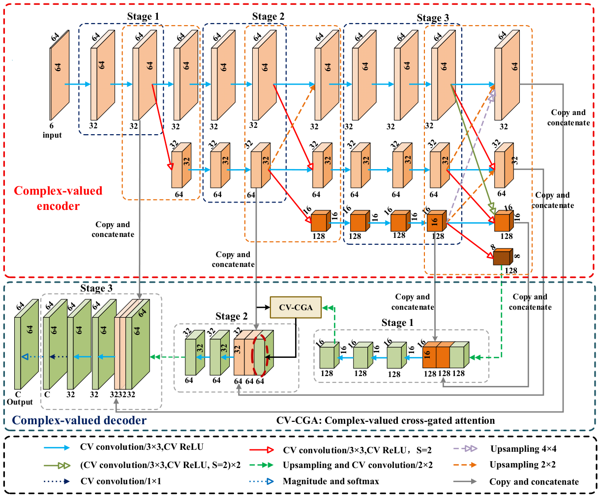
Figure 1. Overall architecture of the proposed complex-valued high-resolution U-Net (CV-HRU-Net) with the complex-valued cross-gated attention (CV-CGA) module.
Remotesensing 18 02947 g001
Figure 2. Architecture of the CV-CGA module.
Remotesensing 18 02947 g002
Figure 3. Pauli RGB images, corresponding ground-truth maps, and class legends for the four datasets. (a) Airborne San Francisco dataset. (b) Airborne Flevoland dataset. (c) Guangzhou subset of the spaceborne AIR-PolSAR-Seg-2.0 dataset. (d) Spaceborne San Francisco dataset. In (d), the red line indicates the spatial boundary separating the test region (above) from the training region (below).
Remotesensing 18 02947 g003
Figure 4. Full-scene segmentation results on the airborne San Francisco dataset. (a) FCN. (b) DeepLabv3+. (c) TransUNet. (d) SegFormer. (e) DSNet. (f) CGRSeg. (g) VWFormer. (h) L-CV-DeepLabv3+. (i) CV-Cap-U-Net. (j) Proposed method. White boxes 1–3: regions of interest selected for qualitative comparison.
Remotesensing 18 02947 g004
Figure 5. Full-scene segmentation results on the airborne Flevoland dataset. (a) FCN. (b) DeepLabv3+. (c) TransUNet. (d) SegFormer. (e) DSNet. (f) CGRSeg. (g) VWFormer. (h) L-CV-DeepLabv3+. (i) CV-Cap-U-Net. (j) Proposed method. Black boxes 1–3: regions of interest selected for qualitative comparison.
Remotesensing 18 02947 g005
Figure 6. Segmentation results on two test patches from the Guangzhou subset of the spaceborne AIR-PolSAR-Seg-2.0 dataset. (a) Fast-SCNN. (b) BiSeNetv2. (c) L-CV-DeepLabv3+. (d) CV-Cap-U-Net. (e) Proposed method. (f) Ground truth. Black box: region of interest selected for qualitative comparison.
Remotesensing 18 02947 g006
Figure 7. Full-scene segmentation results on the spaceborne San Francisco dataset. (a) Fast-SCNN. (b) BiSeNetv2. (c) L-CV-DeepLabv3+. (d) CV-Cap-U-Net. (e) Proposed method. White boxes 1–2: regions of interest selected for qualitative comparison.
Remotesensing 18 02947 g007
Figure 8. Effect of the channel-wise phase-offset bound on overall segmentation performance.
Remotesensing 18 02947 g008
Figure 9. Visualization of decoder features at Stage 2. (a) Ground truth of the input test sample. (b) Decoder features without CV-CGA. (c) Decoder features with CV-CGA.
Remotesensing 18 02947 g009
Figure 10. Visualization of cross-attention and feature recalibration for two test samples. The upper and lower rows correspond to two different samples. (a) Ground-truth maps with the selected query locations. (b) Global attention maps. (c) Attention maps for query 1. (d) Attention maps for query 2. (e) Attention maps for query 3. (f) Correction-strength maps.
Remotesensing 18 02947 g010
Table 1. Ablation Results on the Major Architectural Components (%).
DatasetRV-
U-Net
RV-
HRNet
RV-
CGA
CV-
U-Net
CV-
HRNet
CV-
CGA
mIoUOAMPABF1
Airborne
San Francisco
89.3496.5093.5175.28
92.8497.1295.5780.27
94.4498.3895.8885.94
93.5998.0796.5684.07
97.2198.6498.5791.88
Airborne
Flevoland
96.0099.5698.2592.25
96.4899.6598.6093.44
96.8699.6198.1793.51
97.3899.7598.8693.68
97.7999.7698.9495.41
Spaceborne
AIR-PolSAR-Seg-2.0
(Guangzhou
subset)
71.8595.0676.3788.72
89.6096.3293.7192.18
90.0196.2293.5292.34
90.2296.3793.4392.26
91.3296.8494.1592.74
Spaceborne
San Francisco
94.4197.7997.1985.89
95.3498.2797.6288.71
95.9298.4797.9087.85
96.0398.5797.8988.52
96.6698.7798.4689.13
Note: “✓” denotes selected items.
Table 2. Ablation Results for the internal components of CV-CGA on the Airborne San Francisco Dataset) (%).
BaselineCV-CBAMCV Cross-AttentionAdaptive Gated RecalibrationmIoUOAMPABF1
93.5998.0796.5684.07
94.2198.4595.9586.37
95.3598.5497.6386.76
95.3998.4196.9489.30
96.7698.4797.7891.05
97.2198.6498.5791.88
Note: “✓” denotes selected items.
Table 3. Ablation Results on the Insertion Position of CV-CGA on the Airborne San Francisco Dataset) (%).
Stage 1 Stage 2 Stage 3 mIoU OA MPA BF1
94.3598.5295.8084.85
97.2198.6498.5791.88
96.3298.2897.9390.29
96.3598.4797.8089.37
Note: “✓” denotes selected items.
Table 4. Semantic Segmentation Performance on the Airborne San Francisco Dataset (%).
Class FCN DeepLabv3+ TransUNet SegFormer DSNet CGRSeg VWFormer L-CV-DeepLabv3+ CV-Cap-U-Net Proposed
188.96 ± 0.7870.12 ± 2.5293.66 ± 1.9788.04 ± 1.1892.39 ± 1.2779.20 ± 3.5490.92 ± 0.7092.41 ± 1.0894.72 ± 1.2796.06 ± 0.70
286.34 ± 0.8679.39 ± 2.6291.89 ± 0.7885.93 ± 1.4189.89 ± 0.4175.28 ± 2.9290.45 ± 1.5891.70 ± 1.6894.94 ± 1.1495.59 ± 0.19
395.25 ± 4.7896.20 ± 1.2298.81 ± 0.3898.30 ± 0.1798.44 ± 0.4392.27 ± 4.4697.22 ± 4.1098.54 ± 0.5599.32 ± 0.2999.01 ± 0.18
488.47 ± 5.3260.00 ± 2.8294.09 ± 0.3481.68 ± 2.6592.00 ± 0.8174.61 ± 7.8390.66 ± 1.6190.50 ± 1.0194.55 ± 2.1595.37 ± 0.87
575.81 ± 5.6733.19 ± 6.2685.15 ± 4.6457.76 ± 12.4671.56 ± 11.3456.22 ± 20.1285.78 ± 5.4687.97 ± 5.9186.70 ± 3.6997.27 ± 1.90
mIoU85.45 ± 1.1371.52 ± 1.4992.41 ± 0.8281.79 ± 2.1989.39 ± 1.6177.37 ± 1.0491.68 ± 0.9692.25 ± 1.6195.03 ± 1.1097.21 ± 0.06
OA94.62 ± 0.3689.90 ± 0.6597.30 ± 0.1894.01 ± 0.6996.72 ± 0.1590.62 ± 1.7396.47 ± 0.7497.00 ± 0.6298.46 ± 0.3598.64 ± 0.15
MPA90.57 ± 0.9579.50 ± 0.9395.32 ± 0.6988.09 ± 2.2993.65 ± 0.7186.11 ± 2.2595.32 ± 1.4595.73 ± 0.9597.57 ± 0.4998.57 ± 0.02
BF175.66 ± 1.8061.01 ± 1.4089.50 ± 1.3177.22 ± 2.9281.67 ± 0.6968.25 ± 0.9085.27 ± 0.8984.66 ± 2.1685.71 ± 2.1591.88 ± 0.90
Table 5. Semantic Segmentation Performance on the Airborne Flevoland Dataset (%).
ClassFCNDeepLabv3+TransUNetSegFormerDSNetCGRSegVWFormerL-CV-DeepLabv3+CV-Cap-U-NetProposed
194.15 ± 1.5797.54 ± 1.5590.23 ± 4.2084.19 ± 0.6098.42 ± 0.3762.59 ± 17.0692.84 ± 0.3196.26 ± 0.5594.68 ± 1.2599.01 ± 1.26
286.87 ± 6.1785.67 ± 5.4564.86 ± 18.2277.76 ± 6.9195.60 ± 1.6670.51 ± 11.6494.70 ± 0.2395.67 ± 0.9598.33 ± 1.1695.86 ± 1.68
394.05 ± 1.0191.26 ± 1.9391.86 ± 0.5090.09 ± 0.8794.83 ± 0.8270.75 ± 4.8692.02 ± 1.6895.03 ± 0.4097.19 ± 0.7999.64 ± 0.22
490.77 ± 2.1284.64 ± 3.1568.09 ± 2.1188.82 ± 7.6487.33 ± 2.2133.58 ± 24.6092.47 ± 3.1797.78 ± 1.7897.93 ± 1.6396.68 ± 1.74
591.62 ± 3.3981.89 ± 4.1881.66 ± 3.0289.79 ± 2.5784.76 ± 3.4565.57 ± 11.4892.90 ± 1.0497.53 ± 0.9298.02 ± 0.3896.17 ± 1.55
683.03 ± 5.2787.27 ± 6.2970.68 ± 3.1386.74 ± 3.2395.52 ± 2.9734.02 ± 16.8396.50 ± 0.4798.07 ± 0.4899.30 ± 0.2098.91 ± 0.97
795.70 ± 0.4294.54 ± 2.3790.59 ± 1.7790.51 ± 0.9597.49 ± 0.8768.12 ± 5.3593.57 ± 1.3598.41 ± 0.6898.10 ± 0.9399.11 ± 0.34
884.78 ± 8.7787.43 ± 8.4172.68 ± 10.3284.37 ± 6.5492.10 ± 6.0524.07 ± 12.6154.96 ± 12.1999.19 ± 0.3293.40 ± 8.2299.94 ± 0.03
986.94 ± 2.4866.85 ± 9.0738.30 ± 4.6684.04 ± 3.2781.45 ± 3.030.43 ± 0.4087.38 ± 4.2393.60 ± 1.3996.79 ± 3.3896.15 ± 1.97
1078.70 ± 6.9643.90 ± 6.1264.25 ± 4.6373.64 ± 11.4073.91 ± 11.8729.05 ± 3.6784.76 ± 1.6495.82 ± 3.0797.19 ± 3.5294.27 ± 2.39
1196.95 ± 2.1596.37 ± 2.8184.56 ± 5.3691.13 ± 4.3297.65 ± 1.6921.59 ± 18.6695.92 ± 3.0899.41 ± 0.4499.25 ± 0.7399.83 ± 0.27
1284.37 ± 1.5546.43 ± 6.6778.79 ± 8.1079.54 ± 4.4573.74 ± 12.7918.91 ± 8.4888.73 ± 4.2091.84 ± 2.0696.46 ± 3.1897.28 ± 1.43
1394.93 ± 1.1993.66 ± 1.2190.82 ± 2.2188.35 ± 5.9397.05 ± 1.4136.33 ± 17.5796.91 ± 0.4297.36 ± 1.4398.78 ± 0.2798.71 ± 0.95
1495.07 ± 2.0489.26 ± 7.5887.79 ± 5.5591.47 ± 1.0492.03 ± 1.9728.66 ± 21.5473.49 ± 7.2696.47 ± 0.7896.53 ± 1.3198.08 ± 0.17
1559.36 ± 15.664.54 ± 10.0924.37 ± 9.4114.47 ± 0.8573.90 ± 9.7212.60 ± 11.0882.59 ± 2.9474.35 ± 3.9097.77 ± 0.7495.12 ± 2.67
mIoU88.22 ± 2.1081.88 ± 1.7974.51 ± 1.6781.60 ± 1.2189.05 ± 1.3440.64 ± 1.4588.30 ± 1.2895.34 ± 0.6497.36 ± 0.1197.79 ± 0.34
OA98.71 ± 0.1997.59 ± 0.3197.17 ± 0.1697.75 ± 0.2598.79 ± 0.1964.49 ± 8.5598.42 ± 0.7599.52 ± 0.0599.74 ± 0.0699.76 ± 0.05
MPA93.40 ± 1.7488.29 ± 1.2083.48 ± 1.4187.84 ± 0.6894.22 ± 0.9064.55 ± 12.3294.58 ± 0.5497.90 ± 0.1098.83 ± 0.2698.94 ± 0.11
BF181.23 ± 1.4277.45 ± 3.1270.76 ± 0.9282.22 ± 0.9987.92 ± 1.8336.95 ± 0.9385.27 ± 0.8891.96 ± 1.6094.62 ± 0.7195.41 ± 0.70
Table 6. Semantic Segmentation Performance on the Guangzhou Subset of the Spaceborne AIR-PolSAR-Seg-2.0 Dataset (%).
ClassFast-SCNNBiSeNetv2L-CV-DeepLabv3+CV-Cap-U-NetProposed
188.70 ± 0.4592.95 ± 0.3093.83 ± 0.4195.27 ± 0.4295.20 ± 0.55
284.06 ± 0.1887.72 ± 0.7786.48 ± 0.0388.91 ± 0.3190.59 ± 0.39
374.23 ± 0.7879.97 ± 0.5375.85 ± 0.4983.11 ± 1.6083.32 ± 0.88
485.22 ± 0.2889.46 ± 0.5190.88 ± 0.2191.30 ± 0.4792.09 ± 0.53
592.22 ± 0.1693.76 ± 0.3993.66 ± 0.1594.57 ± 0.2095.39 ± 0.17
mIoU84.89 ± 0.2888.77 ± 0.4088.14 ± 0.2090.63 ± 0.1791.32 ± 0.50
OA94.19 ± 0.1195.70 ± 0.2395.66 ± 0.0196.36 ± 0.1496.84 ± 0.16
MPA91.86 ± 1.9492.69 ± 0.3892.12 ± 0.0194.09 ± 0.4594.15 ± 0.40
BF187.20 ± 0.2290.37 ± 0.3492.66 ± 0.0791.81 ± 1.1092.74 ± 0.37
Table 7. Semantic Segmentation Performance on the Spaceborne San Francisco Dataset (%).
ClassFast-SCNNBiSeNetv2L-CV-DeepLabv3+CV-Cap-U-NetProposed
186.68 ± 0.6292.46 ± 1.4191.04 ± 4.5896.59 ± 0.2696.31 ± 0.82
284.74 ± 1.3788.54 ± 0.6084.29 ± 2.6496.07 ± 0.4896.16 ± 0.64
383.70 ± 1.9388.24 ± 1.4686.41 ± 1.1493.41 ± 0.6094.86 ± 1.24
496.36 ± 2.3796.71 ± 0.1898.81 ± 0.1898.97 ± 0.2299.16 ± 0.09
581.37 ± 7.1282.57 ± 1.2786.76 ± 1.1291.28 ± 0.9993.53 ± 1.11
mIoU87.17 ± 2.1090.01 ± 0.6788.61 ± 1.2596.05 ± 0.1496.66 ± 0.39
OA94.45 ± 1.1595.58 ± 0.2195.54 ± 0.6598.51 ± 0.0598.77 ± 0.10
MPA93.11 ± 0.6695.02 ± 0.4593.91 ± 0.5298.17 ± 0.1798.46 ± 0.29
BF172.66 ± 4.0177.49 ± 1.1172.90 ± 8.9585.44 ± 0.8889.13 ± 1.42
Table 8. Segmentation Performance under Different Channel-wise Phase-Offset Bounds on the Airborne San Francisco Dataset (%).
30°60°90°120°150°180°
mIoU97.2196.2395.1882.4268.1356.5851.32
OA98.6498.1597.5589.4576.9769.3766.28
MPA98.5798.1797.7393.0285.5080.1777.38
BF191.8890.6286.7970.5163.3459.6158.04
Table 9. Model Complexity and Performance on the Airborne San Francisco Dataset.
ModelInputParameters
(M)
FLOPs
(G)
FPSTraining Time
(s/epoch)
Inference latency
(ms/image)
mIoU
(%)
RV-HRU-Net
w RV-CGA
9-channel
real-valued
1.470.69202.2316.504.9494.44
RV-HRU-Net
w RV-CGA
(2 × width)
9-channel
real-valued
5.862.74198.1920.745.0591.35
CV-HRU-Net
w/o CV-CGA
6-channel
complex-valued
4.024.8929.83140.1133.5393.59
CV-HRU-Net
w CV-CGA
6-channel
complex-valued
4.064.9625.25145.7139.6097.21
Disclaimer/Publisher’s Note: The statements, opinions and data contained in all publications are solely those of the individual author(s) and contributor(s) and not of MDPI and/or the editor(s). MDPI and/or the editor(s) disclaim responsibility for any injury to people or property resulting from any ideas, methods, instructions or products referred to in the content.