Surface Subsidence Analysis and Prediction in an Open-Pit Mine Using Time-Series InSAR and a CL-TSF Hybrid Model

Highlights

What are the main findings?

• Time-series InSAR analysis of 70 Sentinel-1A images revealed a continuously evolving subsidence bowl in the Fushun West Open-pit Mine, with a maximum subsidence rate of 143.00 mm/yr and a cumulative displacement of −337.89 mm.
• A hybrid CNN–LSTM time-series forecasting model (CL-TSF) was developed for subsidence prediction, achieving higher accuracy than conventional CNN and LSTM models, with a MAPE of 2.24% and an RMSE of 5.260.

What are the implications of the main findings?

• Rainfall was identified as the dominant external factor controlling surface subsidence, while regional seismic activity exerted only a negligible influence, improving the understanding of mining-induced deformation mechanisms.
• The integrated TS-InSAR and CL-TSF framework enables accurate multi-step forecasting of mining subsidence and provides an effective tool for geohazard early warning, risk assessment, and sustainable mine management.

Abstract

Surface subsidence in mining areas is a widespread, long-term, and slow-onset geological hazard that can induce cascading failures, including slope instability and ground collapse, thereby threatening infrastructure and human safety. Accurate characterization of its spatiotemporal evolution and reliable prediction of future trends are therefore essential for effective mine safety management and hazard assessment. This study investigates an open-pit mine by integrating time-series Interferometric Synthetic Aperture Radar (InSAR) monitoring with a deep learning–based prediction framework. A total of 70 Sentinel-1A synthetic aperture radar (SAR) images acquired between January 2023 and May 2025 were processed to quantify surface deformation. The results reveal a large-scale subsidence funnel, with a maximum subsidence rate of 143.00 mm/yr and a cumulative displacement of −337.89 mm. The observed deformation is controlled by combined effects of rainfall, seismic activity, and local geological conditions. To predict the temporal evolution of subsidence, a hybrid convolutional neural network–long short-term memory (CNN–LSTM) time-series forecasting model (CL-TSF) is proposed. By integrating convolutional feature extraction with long short-term memory–based sequence modeling, the model effectively captures spatial patterns and long-term temporal dependencies. Compared with conventional CNN and LSTM models, the proposed approach achieves superior performance, with a Mean Absolute Percentage Error (MAPE) of 2.24% and a Root Mean Square Error (RMSE) of 5.260. Its robustness is validated through accurate multi-step prediction of the final five deformation periods. These findings provide insights into mining-induced subsidence mechanisms and demonstrate the potential of the proposed framework for dynamic early warning and risk assessment in mining areas.

1. Introduction

Open-pit mining is a key approach for extracting near-surface mineral resources and has long supported global industrial and economic development. However, large-scale excavation significantly disturbs the in situ stress equilibrium of rock–soil masses, rendering mining areas highly susceptible to geohazards such as landslides and surface subsidence, which pose serious threats to operational safety as well as to lives and property [1].

As one of Asia’s largest and longest-operating open-pit coal mines, the Fushun West Open-pit Mine has undergone more than a century of intensive excavation, resulting in complex and evolving geohazard processes that have attracted sustained research attention. Numerous studies have investigated instability mechanisms at this site. Li et al. [2] combined field monitoring with numerical modeling to reveal the multi-mode failure behavior of a soft–hard interbedded anti-dip slope on the northern wall. Sun et al. [3] reconstructed the rainfall-induced landslide of 26 July 2016 using integrated field investigation, laboratory testing, and seepage–stability analysis. Gao et al. [4] quantified the effects of pit-lake formation and water impoundment during mine closure and evaluated their impact on slope stability. Wei et al. [5] retrieved long-term surface deformation time series from multi-temporal InSAR data and analyzed their relationship with precipitation variability. Collectively, these studies demonstrate that surface deformation and slope instability are particularly pronounced at the Fushun West Open-pit Mine, highlighting its value as a representative natural laboratory for mining-related geohazards. Consequently, long-term, high-precision deformation monitoring and reliable prediction of future evolution are essential for effective early warning and sustainable post-mining management.

Traditional land-subsidence monitoring techniques, including leveling, total-station surveys, and Global Navigation Satellite Systems (GNSS), provide high-accuracy point-based measurements but are generally costly, labor-intensive, and spatially sparse. As a result, they are often insufficient for capturing the spatial heterogeneity and temporal evolution of deformation over large and geologically complex areas such as the Fushun West Open-pit Mine [6]. In contrast, Interferometric Synthetic Aperture Radar (InSAR) has emerged as a transformative technology for surface-deformation monitoring due to its wide spatial coverage, high resolution, and all-weather, day–night acquisition capability. To overcome the limitations of conventional Differential InSAR (D-InSAR), including temporal and spatial decorrelation and atmospheric disturbances, time-series InSAR (TS-InSAR) techniques—particularly Persistent Scatterer InSAR (PS-InSAR) and Small Baseline Subset InSAR (SBAS-InSAR)—have been developed [7,8].

These techniques have been widely applied and continuously refined across diverse geohazard settings. Recent advances further demonstrate their robustness in complex environments. For example, Lv et al. [9] employed a phase-gradient stacking method to detect large-scale landslides in the Sichuan–Tibet region, achieving reliable results where ground-based surveys are impractical. Wang et al. [10] used TS-InSAR to monitor deformation at Beijing Daxing International Airport, achieving millimeter-level agreement with in situ observations, thereby confirming its applicability for large-scale infrastructure safety assessment. In coastal reclaimed areas, Pirunjinda et al. [11] integrated InSAR observations with unsupervised machine-learning techniques to assess subsidence hazards and resolve spatial variability. These studies highlight the effectiveness and versatility of TS-InSAR for monitoring deformation associated with urban subsidence, volcanic activity, and mining operations [12].

Despite the availability of high-quality deformation records, monitoring alone is insufficient for effective disaster prevention and mitigation; reliable prediction of future subsidence trends is essential for timely early warning. Mining-induced subsidence is a complex, nonlinear, and non-stationary process governed by coupled geological conditions, mining activities, rainfall, and other external drivers [13]. This complexity limits the applicability of traditional predictive approaches, such as statistical grey models and classical linear time-series methods. Comparative studies by Zhao et al. [14] and Wang et al. [15] demonstrate that these methods often fail to adequately capture nonlinear and non-stationary behaviors, resulting in limited predictive accuracy.

Recent advances in artificial intelligence have enabled deep learning models—particularly long short-term memory (LSTM) networks and convolutional neural networks (CNNs)—to emerge as powerful tools for predicting landslide displacement and mining-induced subsidence due to their capabilities in nonlinear feature extraction and temporal dependency modeling [16]. Early studies leveraged LSTM networks to capture long-term dependencies in deformation time series [17], while subsequent research improved prediction performance through architectural enhancements, such as the attention-based LSTM [18] and the improved mLSTM model [19]. More recently, hybrid CNN–LSTM frameworks have gained increasing attention in InSAR-based deformation prediction by enabling joint extraction of spatial and temporal features. For example, Zhang et al. [20] applied a CNN–BiLSTM model to the Longtantian open-pit coal mine, achieving favorable results, while Yao et al. [21] successfully used a ConvLSTM model to predict spatiotemporal deformation in the Jinchuan mining area. These studies confirm the effectiveness of hybrid deep learning approaches for deformation prediction.

A key challenge in accurate forecasting lies in capturing the multi-scale dynamic characteristics of deformation time series, which typically consist of long-term trends and short-term fluctuations. While traditional single-model approaches can represent overall trends, they often oversmooth short-term variations and may overlook critical precursory signals. Therefore, developing a hybrid predictive framework capable of capturing both components is essential.

This requirement highlights the advantages of integrating CNN and LSTM architectures. In a CNN–LSTM hybrid model, the CNN serves as an efficient feature-extraction module, identifying localized transient patterns (e.g., accelerated subsidence or short-term rebound) and encoding them into high-level representations. These representations are subsequently processed by the LSTM network, which captures long-term temporal dependencies and evolutionary behavior. Compared with more complex spatiotemporal frameworks that rely on multi-source external data to explain spatial heterogeneity [22,23], the CNN–LSTM hybrid approach provides an efficient, data-driven solution by fully exploiting the intrinsic dynamics of InSAR time series, reducing dependence on auxiliary datasets while maintaining strong generalization capability.

In light of the above, this study focuses on the Fushun West Open-pit Mine and integrates TS-InSAR monitoring with a hybrid deep learning model to analyze and predict the spatiotemporal evolution of surface subsidence. SBAS-InSAR is first applied to process SAR images acquired from 2023 to 2025, generating subsidence velocity fields and displacement time series. These results, combined with external factors such as rainfall and seismic activity, are used to investigate the driving mechanisms of subsidence. Subsequently, a hybrid CNN–LSTM time-series forecasting model (CL-TSF) is developed and trained using InSAR-derived data to predict future subsidence trends in key areas. The proposed framework provides an effective and practical solution for high-precision deformation prediction and offers valuable support for geohazard early warning and risk assessment in large-scale open-pit mining regions.

2. Study Area and Datasets

2.1. Study Area Overview

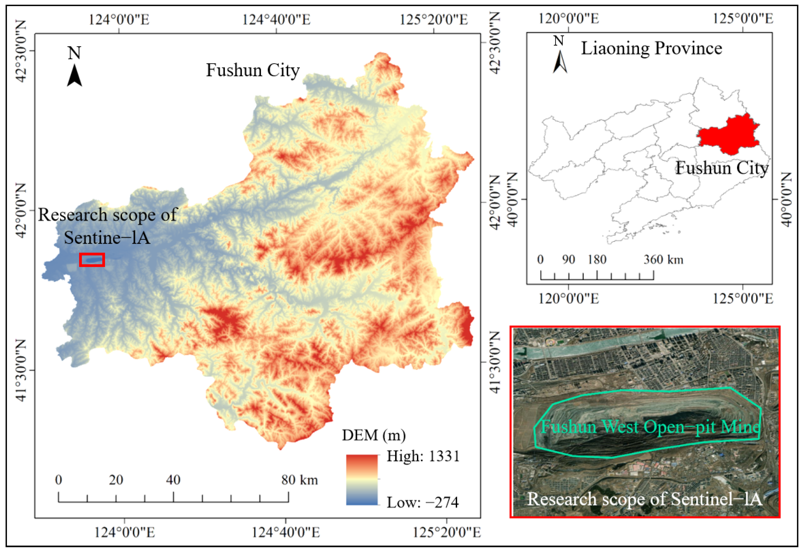
The Fushun West Open-pit Mine is located southwest of Fushun City, Liaoning Province, on the southern bank of the Hunhe River [24] (Figure 1). The study area extends from 123°55′E to 123°59′E and 41°41′N to 41°43′N, with elevations ranging from 50 to 150 m [25]. Geologically, the mine is situated within the Hunhe Fault Zone and is structurally controlled by the Fushun compound syncline. The region is characterized by NE75°-dipping synclinal folds and NEE-dipping reverse faults [26], forming a typical upper-hard/lower-soft lithological assemblage.

More than a century of intensive mining has significantly expanded the pit, which currently extends approximately 6.6 km in the east–west direction and 2.2 km north–south, covering an area of about 14.52 km², with a maximum depth of 420 m below sea level [27]. Prolonged excavation has severely disturbed the geological structure, inducing large-scale ground subsidence and deformation. These processes have resulted in building damage, foundation settlement, and large-scale population relocation. Persistent ground fissures and extensive coal-gangue accumulation further introduce hazards such as spontaneous combustion, soil and water contamination, and environmental degradation. In addition, precipitation infiltration and weathering accelerate slope loosening, increasing the likelihood of secondary geohazards—including landslides and collapses—which pose significant threats to regional ecological systems and infrastructure safety [28].

2.2. Data Sources and SBAS-InSAR Methodology

This study utilizes 70 Sentinel-1A SAR images acquired between 10 January 2023 and 23 May 2025. All images were collected from descending orbit track 105 in Interferometric Wide (IW) swath mode with VV polarization. The SRTM 1 Arc-Second Global DEM (30 m resolution) was used to remove the topographic phase, particularly in areas affected by waste dumps. Precise Orbit Ephemerides (POD), with an accuracy better than 5 cm, were applied to correct orbital phase errors.

The SBAS-InSAR method [29] derives deformation time series by combining multiple differential interferograms with small spatial and temporal baselines. Singular Value Decomposition (SVD) is employed to invert the interferometric network, enabling retrieval of mean deformation rates and displacement time series for coherent targets, thereby improving temporal sampling and spatial coverage.

All SBAS-InSAR processing procedures in this study were executed using the ENVI SARscape platform (version 5.6.2). To ensure the reliability of the interferometric network and minimize decorrelation, key processing parameters were established based on the temporal characteristics of the dataset and the surface conditions of the study area.

The SBAS-InSAR processing workflow consists of five steps:

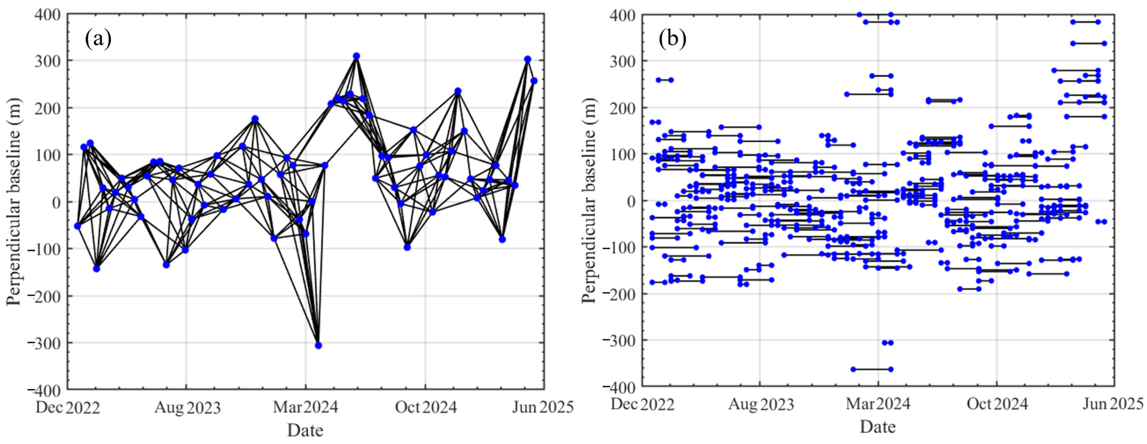
Step 1: To construct a robust and well-connected interferometric network while minimizing spatiotemporal decorrelation, interferometric pairs were selected using a temporal baseline threshold of 90 days and a spatial baseline threshold of 40% of the critical baseline. The image acquired on 29 March 2024 was selected as the super master. The spatial–temporal and temporal baseline distributions are shown in Figure 2a and Figure 2b, respectively.

Step 2: Interferogram generation included flattening, filtering, and phase unwrapping. A multilooking factor of 4:1 was applied to reduce speckle noise and improve phase quality. Goldstein adaptive filtering [30] was used to suppress phase noise, followed by phase unwrapping using the Minimum Cost Flow (MCF) algorithm [31] with a coherence threshold of 0.2. This specific threshold was selected to maximize the retention of valid measurement points while effectively mitigating phase unwrapping errors in low-coherence regions.

Step 3: In the first inversion, 40 high-coherence Ground Control Points (GCPs) located outside deformation zones were selected. Residual phase optimization was applied to estimate and remove constant phase offsets and phase ramps.

Step 4: In the second inversion, linear deformation and residual topographic effects were removed from the unwrapped phase. The remaining phase, containing the Atmospheric Phase Screen (APS) and nonlinear deformation, was processed using temporal high-pass and spatial low-pass filtering to separate APS and extract nonlinear deformation, yielding the final deformation time series.

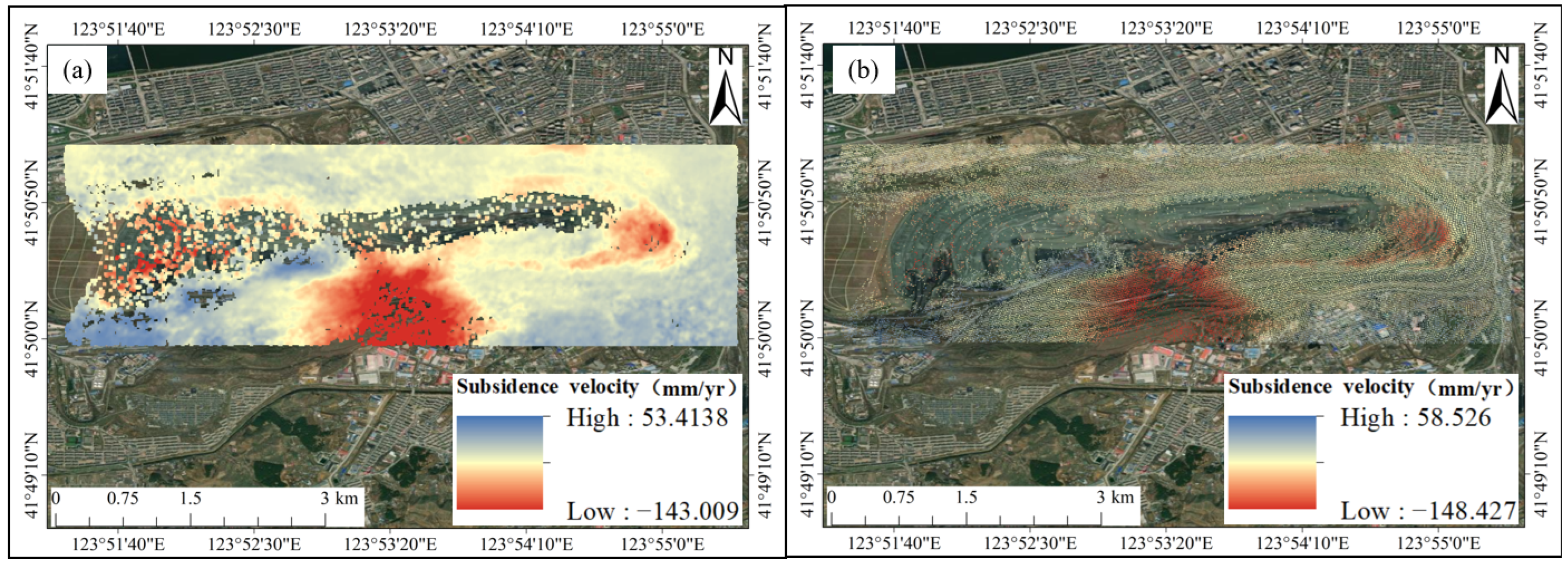
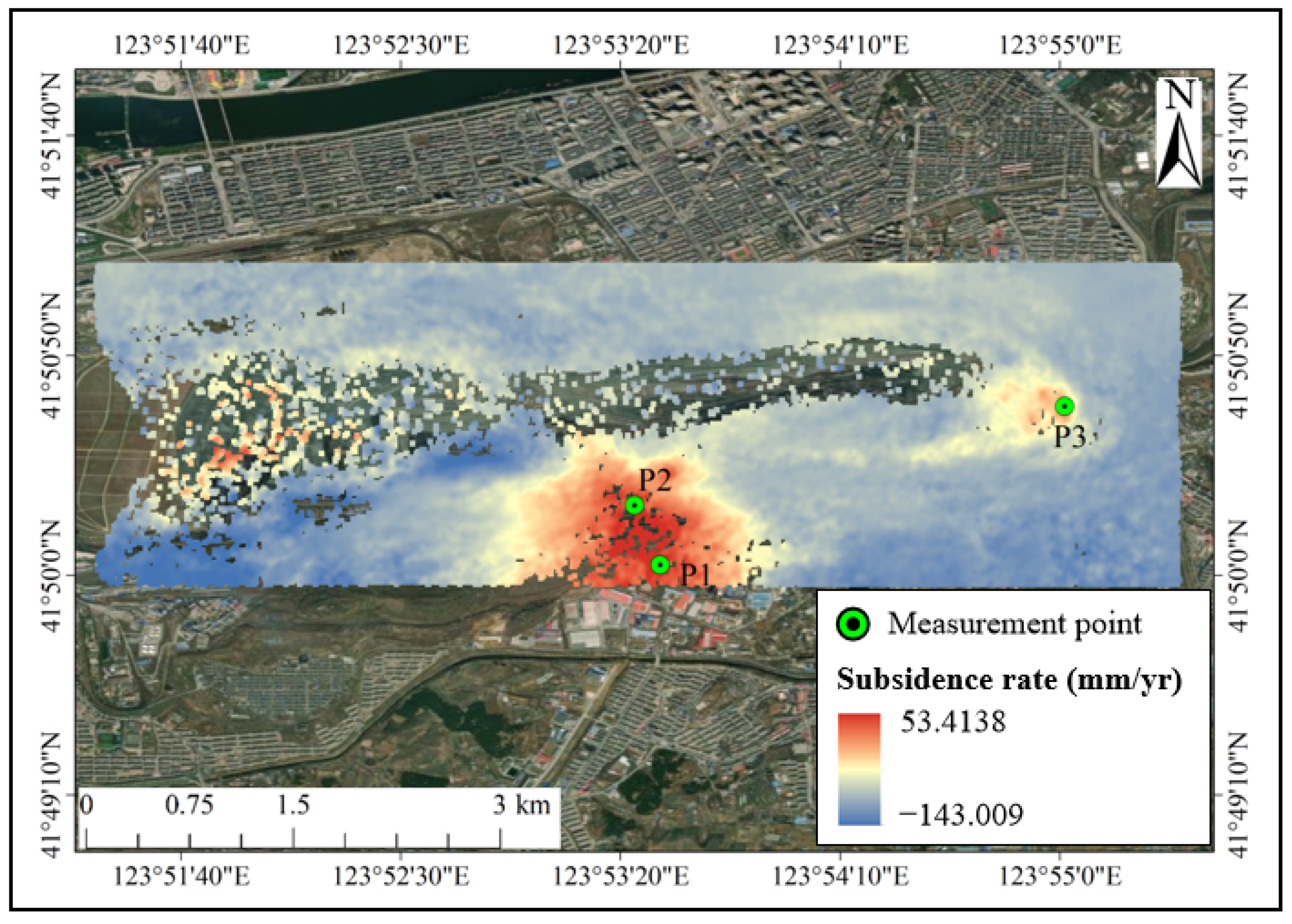
Step 5: The inversion results were geocoded to the GCS-WGS-84 coordinate system using the DEM as a reference. Line-of-sight (LOS) deformation and mean deformation rates were projected and geocoded, with the resulting velocity field shown in Figure 3a.

2.3. Validation of Data Accuracy

To verify the reliability of the SBAS-InSAR results, an independent time-series deformation analysis was conducted using the PS-InSAR technique applied to the same Sentinel-1A dataset for cross-validation. The PS-InSAR method identifies highly coherent point targets (coherence ≥ 0.75 in this study). Given the continuous surface disruption and complex topography inherent to the Fushun West Open-pit Mine, temporal and spatial decorrelation is significant, resulting in spatially sparse PS measurements [32]. To maintain data fidelity and avoid introducing artifacts from interpolation algorithms [33], the original PS points are directly visualized without any smoothing or interpolation (Figure 3b). Although spatially sparse, these highly reliable, non-interpolated permanent scatterers serve as precise anchor points that strongly corroborate the broader deformation patterns captured by the SBAS-InSAR approach.

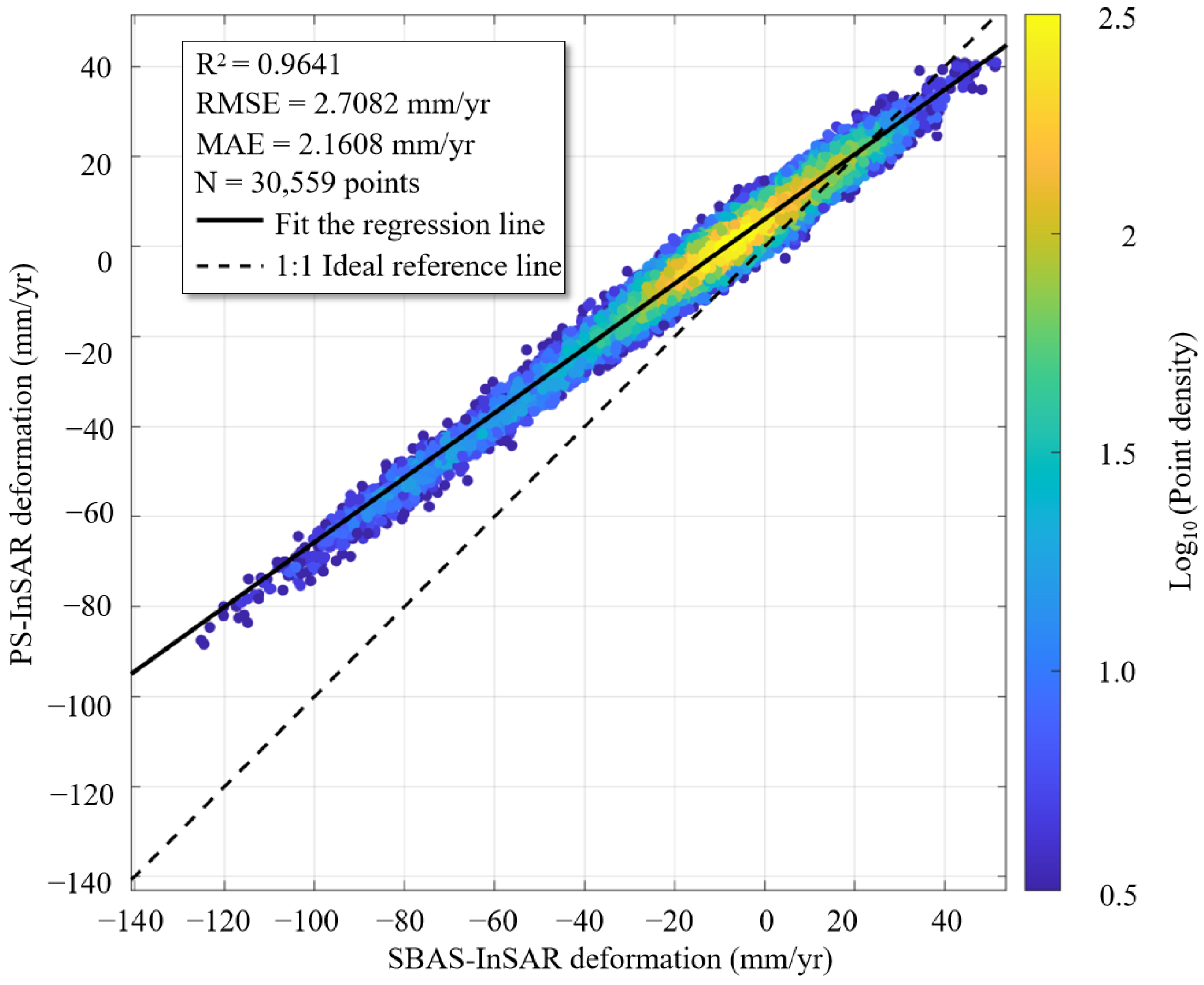
For a more rigorous evaluation, point-to-point cross-validation was performed using the original, non-interpolated datasets. A strict Nearest Neighbor (NN) spatial matching strategy was adopted. Specifically, each PS point was matched exclusively to its spatially closest SBAS observation point within a maximum search radius of 10 m. In rare instances of spatial ambiguity—where multiple equidistant SBAS pixels were located at the exact same minimum distance to a single PS point—the pair with the minimum deformation-rate difference was selected merely as a secondary tie-breaking criterion. Following this rigorous matching strategy, a total of 30,559 valid homologous point pairs were successfully extracted (denoted by N = 30,559 in Figure 4). This substantially large sample size (N) provides a strong statistical foundation for the linear regression analysis. It effectively mitigates the impact of random outliers and ensures high statistical significance, thereby guaranteeing the robustness and credibility of the derived validation metrics (e.g., R², RMSE, and MAE).

Regression analysis of the matched pairs (Figure 4) demonstrates strong consistency between the two methods. The coefficient of determination (R² = 0.9641) indicates excellent agreement in deformation patterns and magnitudes. The low Root Mean Square Error (RMSE = 2.7028 mm/year) and Mean Absolute Error (MAE = 2.1608 mm/year) further confirm minimal discrepancies. These results indicate that, despite differences in scatterer selection mechanisms, the deformation rates derived from SBAS-InSAR and PS-InSAR are highly consistent, validating the robustness and reliability of the SBAS-InSAR results.

It should be noted that incorporating independent ground-based measurements (e.g., GNSS or leveling data) is typically the optimal approach for validating the absolute accuracy of InSAR results. However, the study area, Fushun West Open-pit Mine, is a strictly controlled industrial and mining site. The in situ GNSS monitoring data and geological surveying records are classified as confidential. Due to these strict data security regulations, obtaining concurrent ground-truth measurements for this study was unattainable. Consequently, we relied on the rigorous point-to-point cross-validation between two independent InSAR time-series methodologies. While the absence of ground data limits the assessment of absolute geometric accuracy, the substantial statistical agreement (N = 30,559, R² = 0.9641) between SBAS-InSAR and PS-InSAR provides strong confidence in the relative accuracy and the overall reliability of the identified spatiotemporal deformation patterns.

To ensure a rigorous and unbiased comparison, identical Ground Control Points (GCPs) were utilized as the spatial reference for both the SBAS and PS-InSAR processing workflows. Furthermore, consistent spatial filtering strategies were applied to minimize methodological discrepancies. As shown in the updated Figure 3, the deformation velocity fields derived from both methods exhibit exceptional spatial and numerical consistency. The maximum subsidence rate detected by SBAS-InSAR is −143.00 mm/yr, while PS-InSAR captures a nearly identical maximum rate of −148.42 mm/yr. This minor difference (approximately 5.4 mm/yr) falls well within the acceptable error margin for InSAR applications in extreme deformation environments, thereby mutually validating the absolute reliability of both operational methods and robustly justifying the use of these datasets for the subsequent deep learning predictive models.

3. Subsidence Mechanisms and Deformation Analysis

3.1. Surface Subsidence Analysis

The SBAS-InSAR–derived deformation field reveals pronounced spatial heterogeneity and sustained ground activity across the Fushun West Open-pit Mine. A well-defined, large-scale subsidence bowl has developed within the pit and along its southern slope. The central zone exhibits the most intense deformation, with annual subsidence rates ranging from −98.33 to −143.00 mm/yr (Figure 3a) and a maximum cumulative displacement of −337.89 mm (Figure 5). Subsidence gradually decreases outward from the center, reflecting progressive stress release induced by long-term mining and the associated downward movement of rock masses.

In contrast, localized uplift is observed along the southeastern and eastern margins, with maximum annual rates of 53.41 mm/yr and cumulative uplift up to 119.61 mm. This uplift is likely associated with compaction within waste dumps or stress readjustment following excavation-induced unloading. Overall, the deformation-rate field and cumulative displacement patterns are highly consistent, delineating the current active deformation regime. Notably, the persistent high-rate subsidence along the southern slope indicates a critical stability concern and elevated geohazard risk.

3.2. Spatiotemporal Evolution of Surface Subsidence

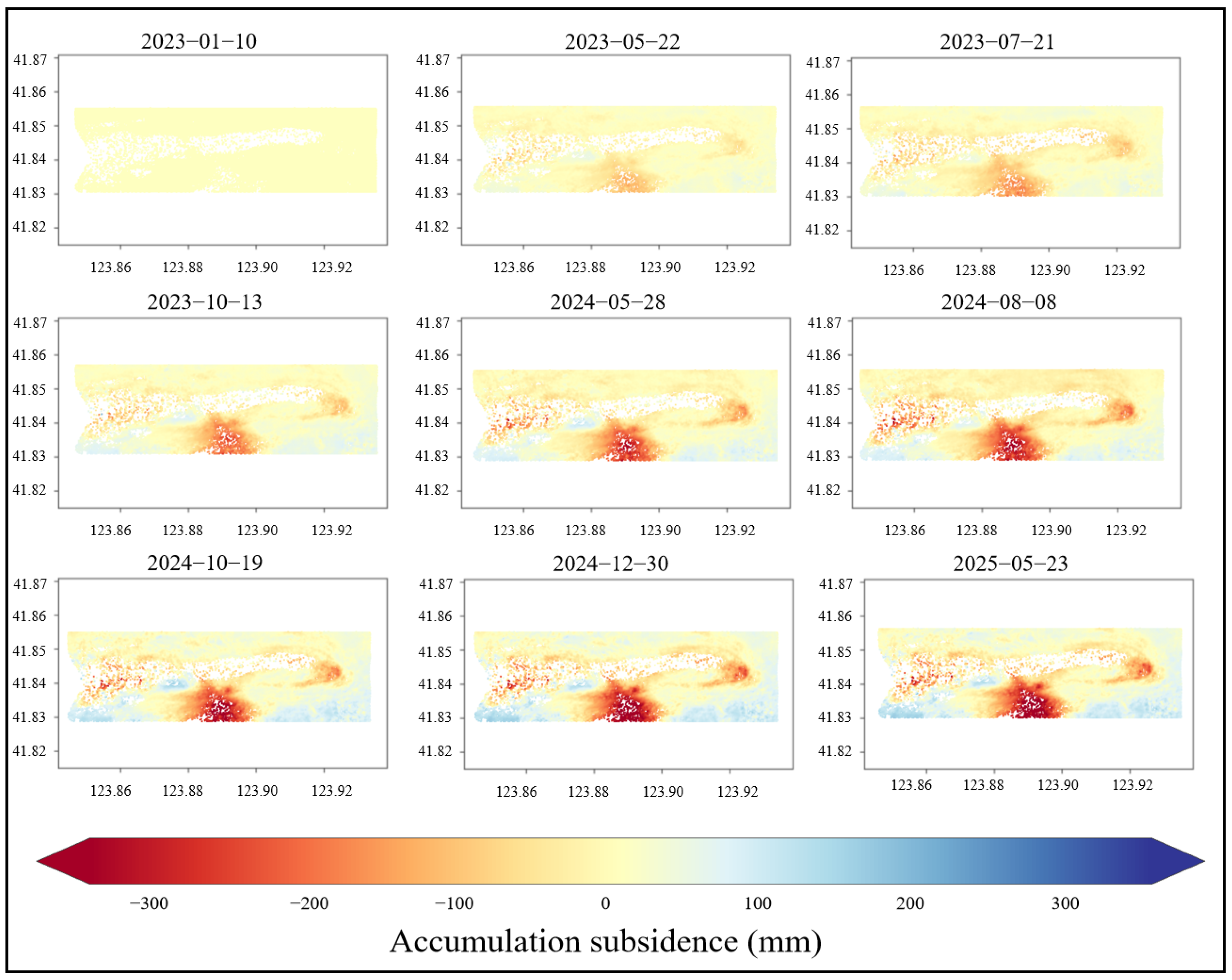
To characterize the spatiotemporal evolution of surface deformation at the open-pit mine, the image acquired on 10 January 2023 was selected as the reference (with cumulative deformation set to zero), and a continuous time-series dataset was generated through 23 May 2025. To clearly reveal the extreme deformation centers previously masked by a narrow color scale, the color range was expanded (i.e., −350 to 350 mm). Within this updated scheme, warm colors (red) indicate surface subsidence moving away from the satellite, while cool colors (blue) represent surface uplift. Based on these settings, the spatiotemporal evolution map of cumulative deformation was produced (Figure 5). By integrating Figure 3a and Figure 5, several key characteristics can be identified:

(1)

Spatiotemporal heterogeneity and strong localization of deformation. Surface deformation exhibits pronounced spatial heterogeneity and is highly localized rather than uniformly distributed across the mining area. A distinct subsidence bowl has developed in the south-central sector (123°53′0″E–123°54′10″E; 41°49′30″N–41°50′10″N). Its irregular geometry suggests that vertical goaf instability is coupled with lateral creep of slope materials toward the pit interior. The bowl center experiences the most severe deformation, with a maximum cumulative subsidence of −337.89 mm, decreasing progressively toward the periphery. In contrast, the northern and far-field areas remain largely stable, with localized uplift reaching up to 119.61 mm, highlighting the high-risk nature of the southern subsidence core.

(2)

Dynamic evolution of an active subsidence bowl. The temporal evolution reflects the full development cycle of an active geohazard. During the initial latency stage (January–June 2023), deformation signals were weak and scattered. From July 2023 to early 2024, subsidence accelerated markedly, with the core area intensifying and expanding, indicating the formation of a well-defined subsidence bowl. Since early 2024, the zone has remained in a sustained high-activity state, with annual subsidence rates reaching up to −143 mm/yr and no evidence of attenuation. This indicates a continuously evolving hazard source that poses a significant structural threat to overlying industrial facilities.

(3)

High deformation gradients at the bowl margins. A pronounced deformation gradient is observed at the bowl margins, transitioning from more than −200 mm at the center to less than −60 mm within a horizontal distance of less than 1 km. This sharp gradient induces strong differential settlement, forming zones of stress concentration where tensile and shear stresses accumulate in the surface and shallow strata. These conditions favor the development of secondary hazards, including surface cracking, differential foundation failure, road deformation, and pipeline rupture. The color-transition zones at the bowl edges therefore delineate the most vulnerable areas for surface damage.

(4)

Divergent deformation modes and hazard mechanisms. A comparative analysis reveals two distinct deformation modes on the southern and northern slopes. The southern slope exhibits rapid, localized “funnel-type” subsidence, associated with a high risk of sudden collapse and rapid infrastructure failure; mitigation strategies should emphasize emergency response, evacuation, and stabilization measures such as grouting. In contrast, the northern slope displays slow but large-scale “creep-type” deformation (−10 to −48 mm/yr). Although the deformation rate is lower, the larger affected mass implies a potential for catastrophic, slope-scale failure. Accordingly, risk mitigation on the northern slope should focus on long-term monitoring and comprehensive engineering measures, including slope unloading and the installation of anti-slide structures.

3.3. Influence of Rainfall on Surface Subsidence

Before delving into the dominant hydro-mechanical drivers, an initial exclusionary evaluation of regional seismic activity was conducted [34,35]. Analysis utilizing Ground Motion Prediction Equations (GMPEs) and linear regression revealed that peak ground acceleration (PGA) and peak ground velocity (PGV) exhibited negligible correlation with short-term post-seismic subsidence (R² = 0.014 and 0.005, respectively) [36,37]. Given the relatively low magnitude and distant epicenters of recorded events during the observation period, regional seismicity constitutes only a minor external perturbation with negligible influence on the mine’s overall deformation [38]. Consequently, this factor was excluded from the subsequent predictive framework, allowing the analysis to focus entirely on the primary driving factors. To elucidate the coupling between precipitation and surface deformation in the Fushun West Open-pit Mine, a comprehensive analysis was conducted. High-resolution SBAS-InSAR processing of time-series radar imagery yielded a millimeter-precision deformation record for 2023–2024. To facilitate multi-source data integration, the InSAR-derived deformation series was subsequently aligned with monthly precipitation data from three monitoring stations (P1, P2, and P3) obtained from the National Tibetan Plateau Data Center (Figure 6). These preprocessing steps established a robust foundation for the ensuing quantitative assessments.

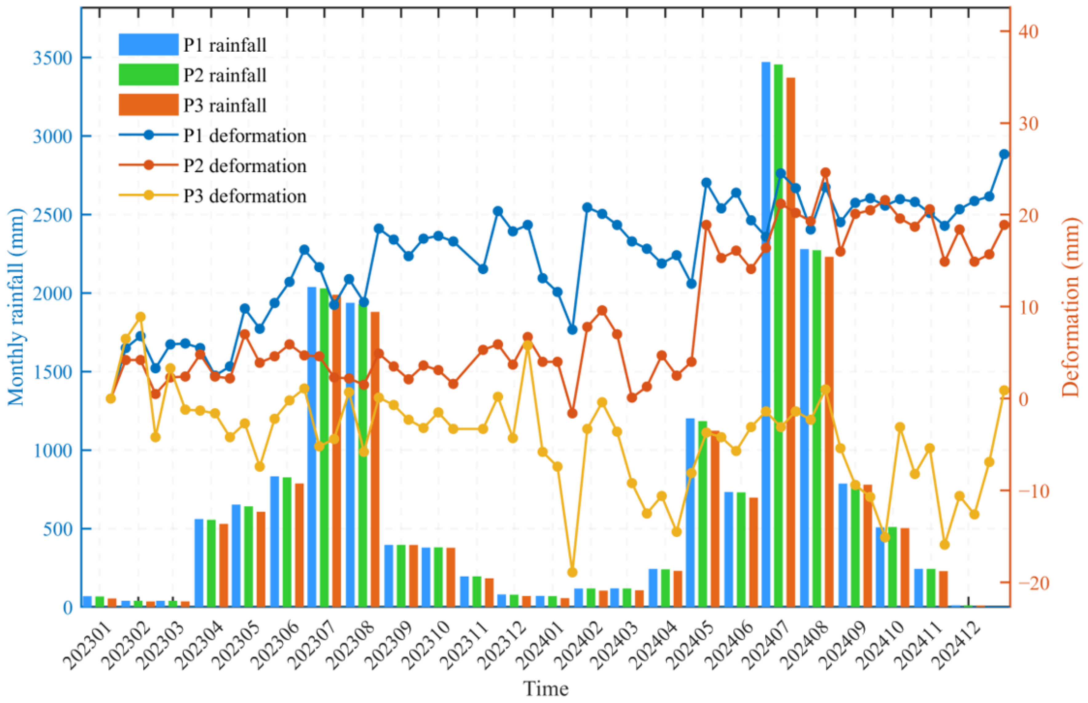
A quantitative comparison between the deformation time-series curves and the precipitation histograms (Figure 7) reveals a clear seasonal correspondence, indicating that precipitation is a primary external control on surface deformation in the mining area. Precipitation influences not only the magnitude and rate of deformation but also its spatiotemporal evolution, with the hydro-mechanical coupling becoming particularly evident under extreme rainfall conditions.

In July 2024, cumulative precipitation reached 3487.6 mm—a recent peak—during which deformation at P1 and P2 accelerated to approximately 27 mm and 22 mm, respectively, while P3 rebounded sharply from −10 mm to nearly 0 mm, demonstrating a synchronous response to intense rainfall. A comparable pattern occurred in summer 2023 (June–September), when cumulative precipitation exceeded 2000 mm. Over this interval, displacement at P1 and P2 increased from roughly 15 mm to about 25 mm (with P2 peaking at 20 mm in August), whereas P3 progressively recovered from −5 mm to 0 mm. These observations collectively indicate that heavy precipitation markedly enhances subsidence rates and induces consistent but spatially variable deformation responses across monitoring points.

To statistically quantify the linear relationship between precipitation and surface deformation, the Pearson correlation coefficient was employed for detailed analysis [39,40]. The coefficient is defined as follows:

$$r={\displaystyle \frac{{\displaystyle \sum _{i=1}^n\left(x_i-\overline{x})(y_i-\overline{y}\right)}}{\sqrt{{\displaystyle \sum _{i=1}^n{(x_i-\overline{x})}^2}}\cdot \sqrt{{\displaystyle \sum _{i=1}^n{(y_i-\overline{y})}^2}}}}$$

(1)

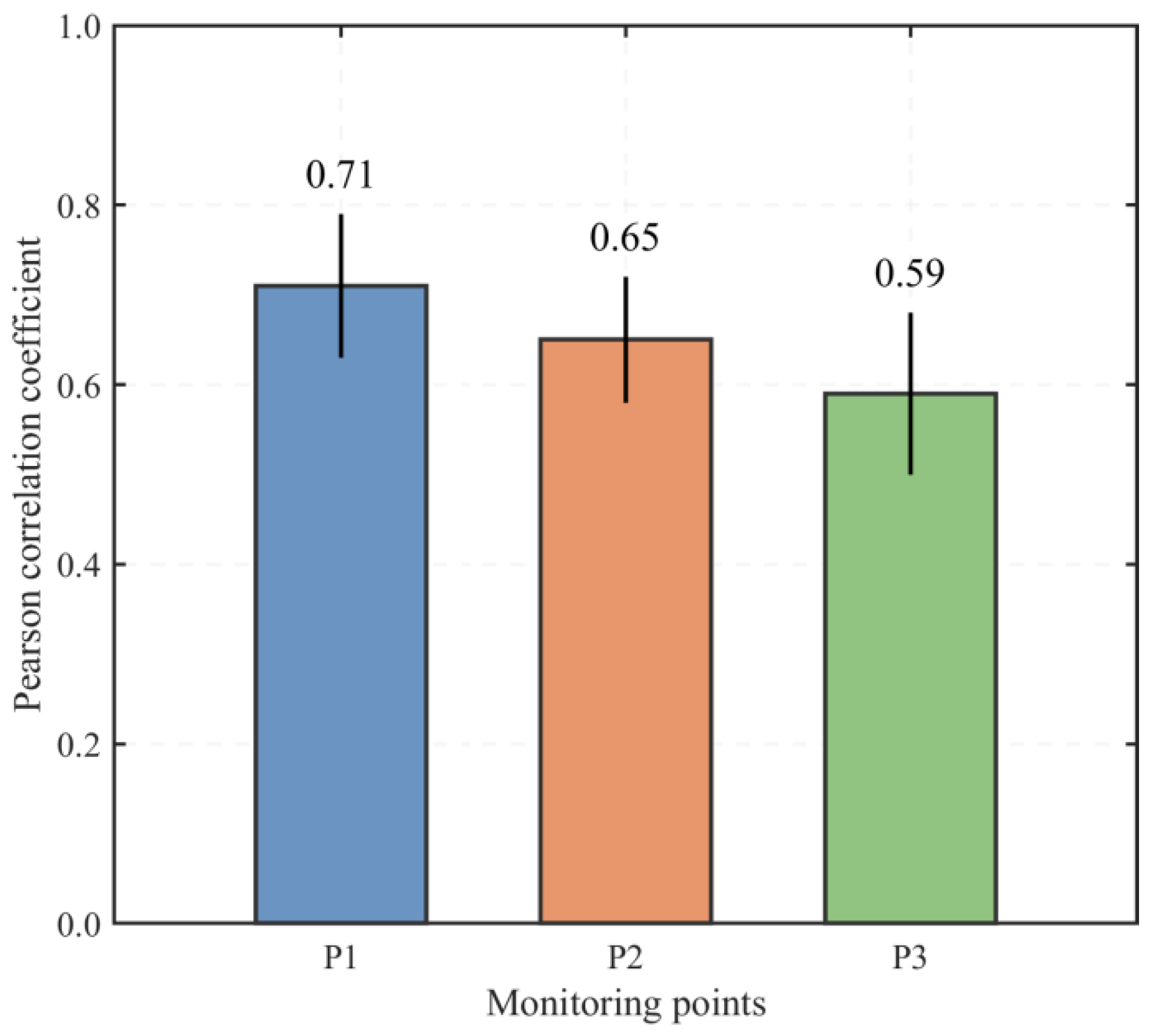
where x_i and y_i represent the observed precipitation and deformation at the i-th time step, and $\overline{x}$ and $\overline{y}$ denote their respective mean values. The coefficient ranges from −1 to 1, with values approaching ±1 indicating a stronger correlation; positive values denote a positive correlation, whereas negative values indicate the opposite. As shown in Figure 8, the Pearson correlation coefficients at P1, P2, and P3 are 0.71, 0.65, and 0.59, respectively. All coefficients passed the significance test, indicating statistically significant moderate-to-strong positive correlations. While these values do not exceed the conventional threshold for strict linear “high correlation” (r > 0.8), they are highly significant within the context of complex geotechnical systems. Mining-induced subsidence is a nonlinear process governed by multiple coupled factors, where the response to precipitation involves complex temporal dynamics, such as delayed surface runoff infiltration and cumulative pore water pressure variations. Given these inherent hydro-mechanical complexities and time-lag effects, achieving a correlation coefficient of 0.71 provides robust quantitative evidence that precipitation acts as a primary external driver of surface deformation in the study area.

It is important to note that the deformation response to precipitation is not instantaneous but exhibits clear time-lag effects and seasonal variability. This time-lag effect can be attributed to the slow infiltration process of surface runoff into the fractured rock mass. The progressive accumulation of infiltrating water gradually elevates the pore water pressure and softens the weak structural planes, eventually leading to delayed macroscopic deformation. Although the Pearson correlation coefficient primarily indicates a strong statistical correlation rather than strict causality, this consistent seasonal time-lag strongly supports precipitation as a dominant external triggering mechanism. For example, although precipitation at P1 peaked during July–August 2023 (monthly rainfall exceeding 2000 mm), the corresponding deformation maximum (~25 mm) occurred in September, indicating a response delay of one to two months. As the region transitioned into the autumn–winter dry season (October–December 2023), cumulative deformation at P1 decreased from 25 mm to approximately 18 mm, reflecting a distinct seasonal rebound.

The combined effects of delayed response and cumulative loading are particularly evident at P3. After reaching a deformation minimum of ~−15 mm in January 2024, P3 exhibited a notable rebound of 10 mm during the dry month of February, despite virtually no precipitation, recovering to −5 mm. This behavior indicates that deformation at P3 is influenced not only by individual rainfall events but also by cumulative precipitation and antecedent hydrological conditions [41]. This observation aligns with established findings on rainfall-induced landslides, where precipitation can function as both a direct trigger and a progressive weakening mechanism for rock and soil masses.

The differential deformation responses among the monitoring points highlight the influence of local geological and hydrological settings. Both P1 and P2, located within the subsidence-prone zone, exhibited markedly higher sensitivity to precipitation than P3, situated in a more peripheral area. During the 2023 rainy season (June–September), cumulative subsidence at P1 and P2 increased by ~10 mm, whereas P3 showed a rebound of ~5 mm (from −5 mm to 0 mm). This contrast became more pronounced during the extreme rainfall event of July 2024: P1 subsided by ~9 mm (18 mm to 27 mm), while P3 displayed an opposite rebound of ~12 mm (−12 mm to near 0 mm). Such divergent deformation patterns underscore the controlling roles of local lithology, fracture-network characteristics, and groundwater recharge pathways at each site.

In summary, this study verifies the physical mechanism by which precipitation accelerates slope subsidence through the increase in pore water pressure and the consequent reduction in effective stress and shear strength in soil and rock masses. It also highlights the nonlinear and spatially heterogeneous nature of this hydro-mechanical process. The use of multi-temporal SBAS-InSAR data enables dynamic characterization of the spatiotemporal evolution of surface deformation and quantification of the relationship between precipitation thresholds and subsidence rates. This integrated framework provides significant value for early warning of slope instability in open-pit mines. By coupling high-resolution precipitation records with InSAR-derived deformation time series, cumulative and time-lag effects can be effectively captured, allowing for timely identification of potential high-risk periods. The findings not only support disaster risk management in the Fushun West Open-pit Mine but also offer methodological guidance for enhancing operational safety in other large-scale mines with similar geological settings. Future work incorporating numerical modeling and groundwater-level monitoring will further refine the quantitative understanding of precipitation–deformation coupling and contribute to the development of more accurate hazard prediction and risk mitigation strategies [6,42,43].

3.4. Influence of Geological Conditions on Surface Subsidence

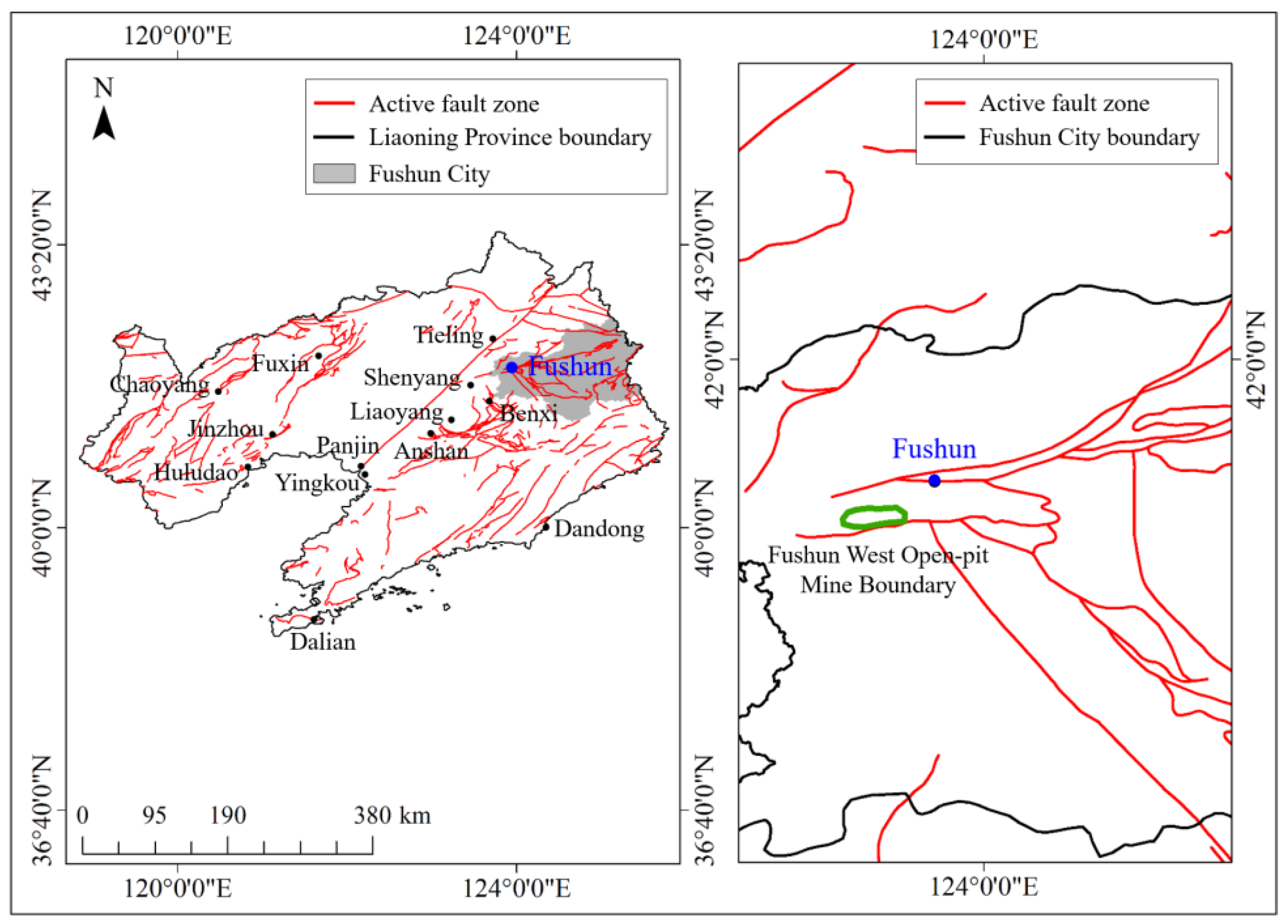
The surface subsidence at the Fushun West Open-pit Mine is not a uniform response to mining-induced unloading; rather, its deformation patterns, magnitudes, and spatial distribution are fundamentally controlled by the geological structural framework at both regional and mine scales. Regionally, the mine lies within a tectonic domain of Liaoning Province characterized by densely developed active faults (Figure 9). It is strongly influenced by the northern extension of the Tan-Lu Fault Zone and its subsidiary Hunhe Fault [44]. This structural inheritance provides the pre-existing tectonic foundation that governs the large-scale deformation regime of the mine [45].

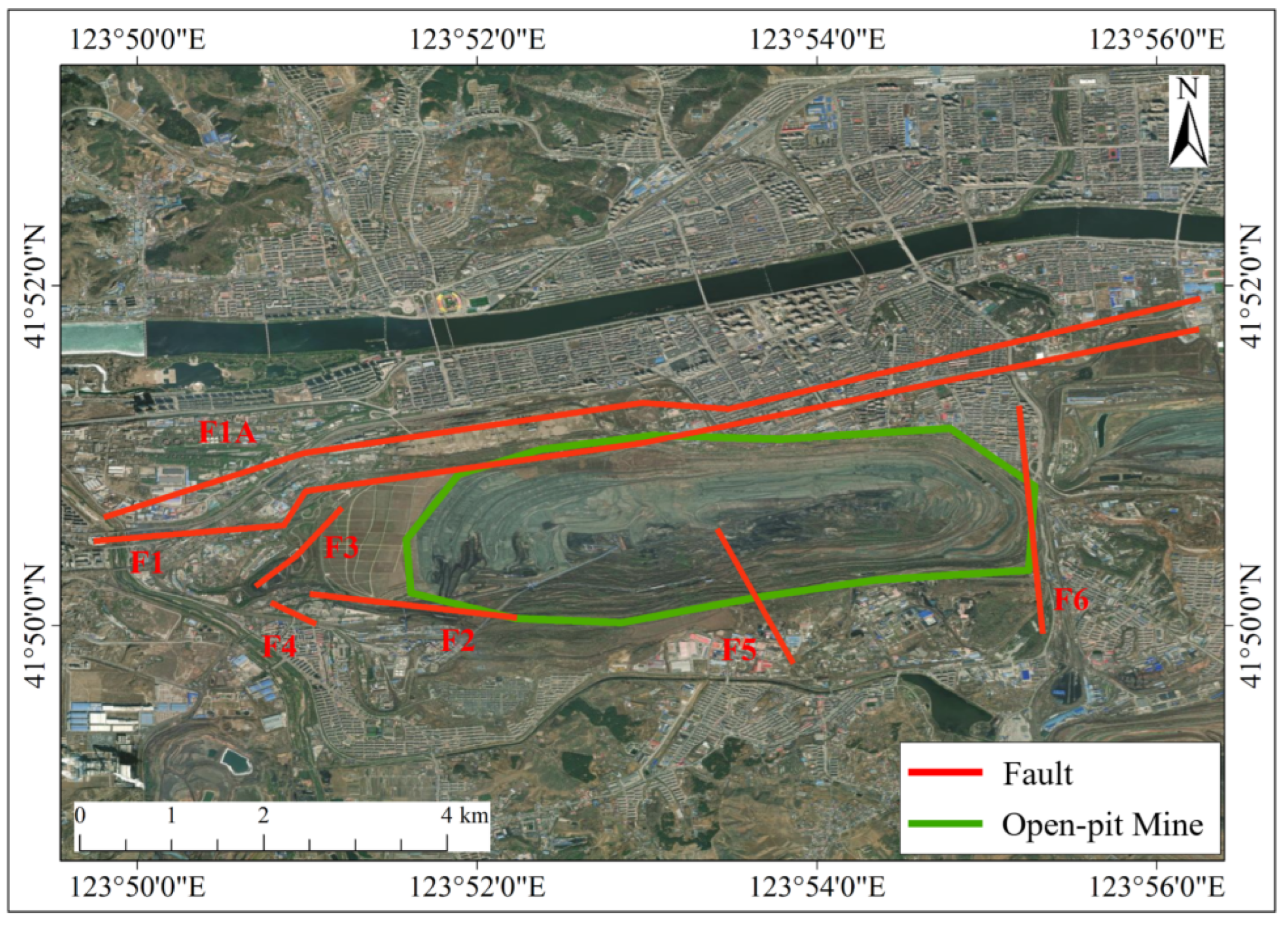
At the mine scale, structural control becomes more explicit. As shown in Figure 10, the open pit is intersected or bounded by a series of active faults with varying orientations. The stability of the northern slope is primarily controlled by the NE–SW-striking Hunhe Fault (F1) and the nearly E–W-striking faults F3 and F4, whereas deformation on the southern slope is closely associated with secondary structures such as F2 and F5. These long-lived fault zones constitute mechanically weakened surfaces with reduced strength [46]. Once mining disturbs the original in situ stress equilibrium, these inherited faults transform from passive geological features into preferential pathways for stress concentration and strain release, thereby becoming key structural elements that actively control surface deformation [3].

The controlling influence of geological structures on subsidence deformation is directly supported by the SBAS-InSAR results (Figure 3a). The non-uniform, block-like and strip-like subsidence patterns observed at the surface correspond closely to the geometry of the underlying fault system. The main subsidence center, with a maximum rate of −143.00 mm/yr, is spatially constrained by multiple intersecting faults including F1, F2, F3, and F5. This structural control is particularly evident near the F1 fault zone, where closely spaced subsidence contours delineate a pronounced deformation gradient, highlighting the role of the fault as a dominant deformation boundary. These characteristics demonstrate that the mine does not exhibit a simple, continuous subsidence basin, but instead reflects a typical “block–fault kinematic” pattern, in which fault-bounded rock masses undergo differential subsidence, slip, and rotation [47]. Within this framework, the fault system plays a dual role: as a kinematic boundary, it provides low-resistance slip surfaces that facilitate relative block movement; and as a hydraulic conduit, it strongly influences subsurface seepage pathways [48]. Mining-induced groundwater drawdown further weakens fault planes through reduced effective stress, enhancing or accelerating shear slip along these structurally weakened zones [49].

In conclusion, the fault system within and around the Fushun West Open-pit Mine functions not as a passive geological backdrop but as the primary structural framework governing the present surface deformation pattern. This controlling role is clearly substantiated by the SBAS-InSAR results: the block-like, highly non-uniform subsidence distribution is effectively a surface manifestation of the mine’s underlying “block–fault kinematics.” The fault network dictates the potential failure modes and deformation pathways, while also constraining the position of subsidence centers, the geometry of the subsidence basin, and the occurrence of sharp deformation gradients. These observations demonstrate that the fundamental mechanism driving surface deformation arises from the interaction between mining-induced stress redistribution and the inherited tectonic fault architecture. It is this interaction that establishes both the structural foundation and the intrinsic deformation mechanism responsible for the observed mining-related subsidence.

4. Predictive Methods for Surface Subsidence

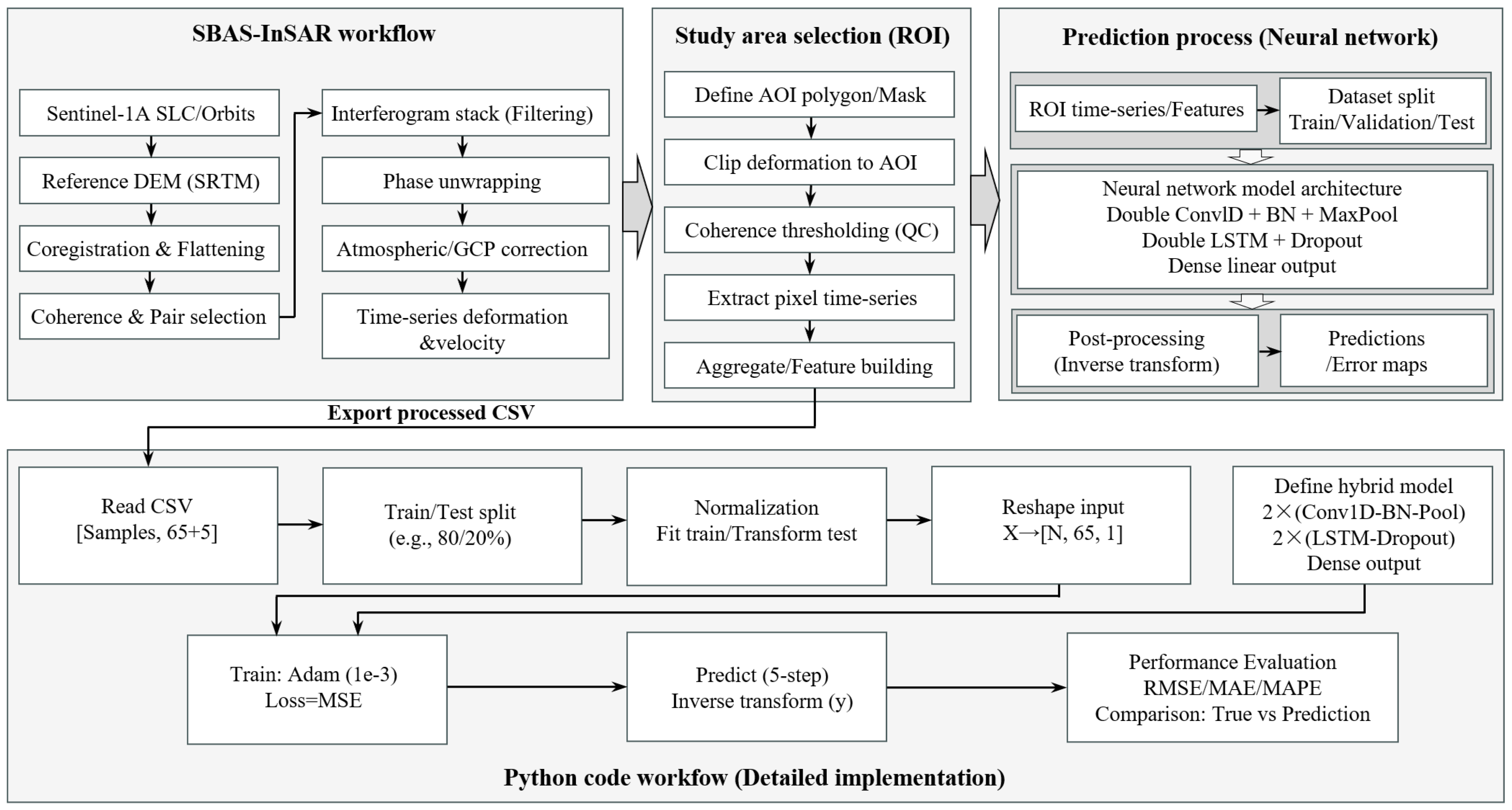
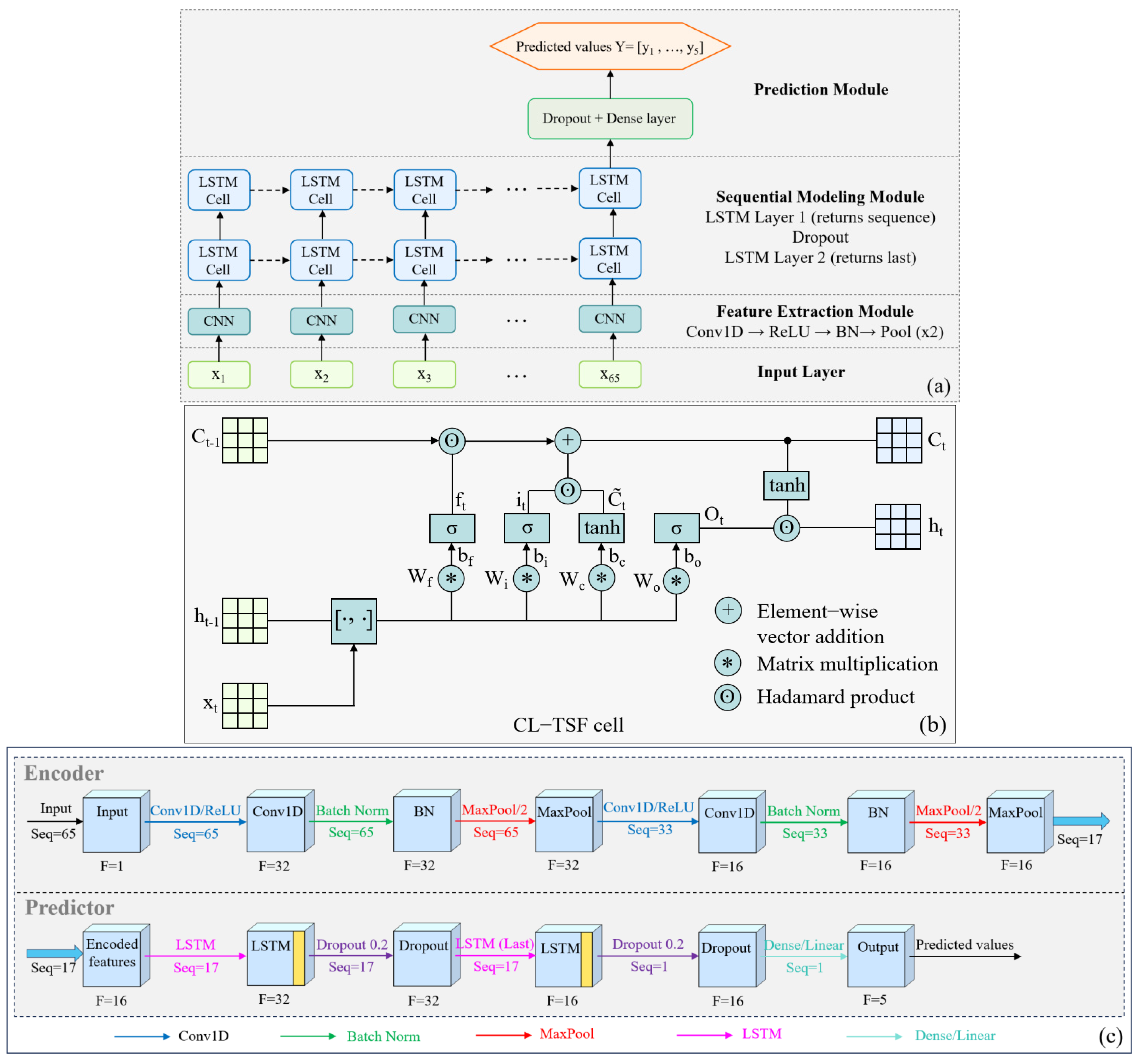
To achieve high-precision forecasting of complex time-series data, this study develops a hybrid deep learning model, CL-TSF (Convolutional–LSTM for time-series forecasting). The model integrates a one-dimensional convolutional neural network (1D-CNN) with an LSTM network within a unified end-to-end framework. This architecture leverages the strength of CNNs in extracting local temporal features and the capability of LSTM networks to capture long-term dependencies in sequential data. The overall workflow of the CL-TSF model, from data input to prediction output, is illustrated in Figure 11.

4.1. Data Preprocessing and Supervised Sample Formulation

The original dataset was obtained using the SBAS-InSAR technique, providing a time-series cumulative surface subsidence field for the study area. It comprises 70 epochs derived from SAR scenes acquired between January 2023 and May 2024. As the raster-formatted SBAS-InSAR outputs cannot be directly used in the CL-TSF model, which requires discrete time-series inputs, data conversion and quality optimization were necessary.

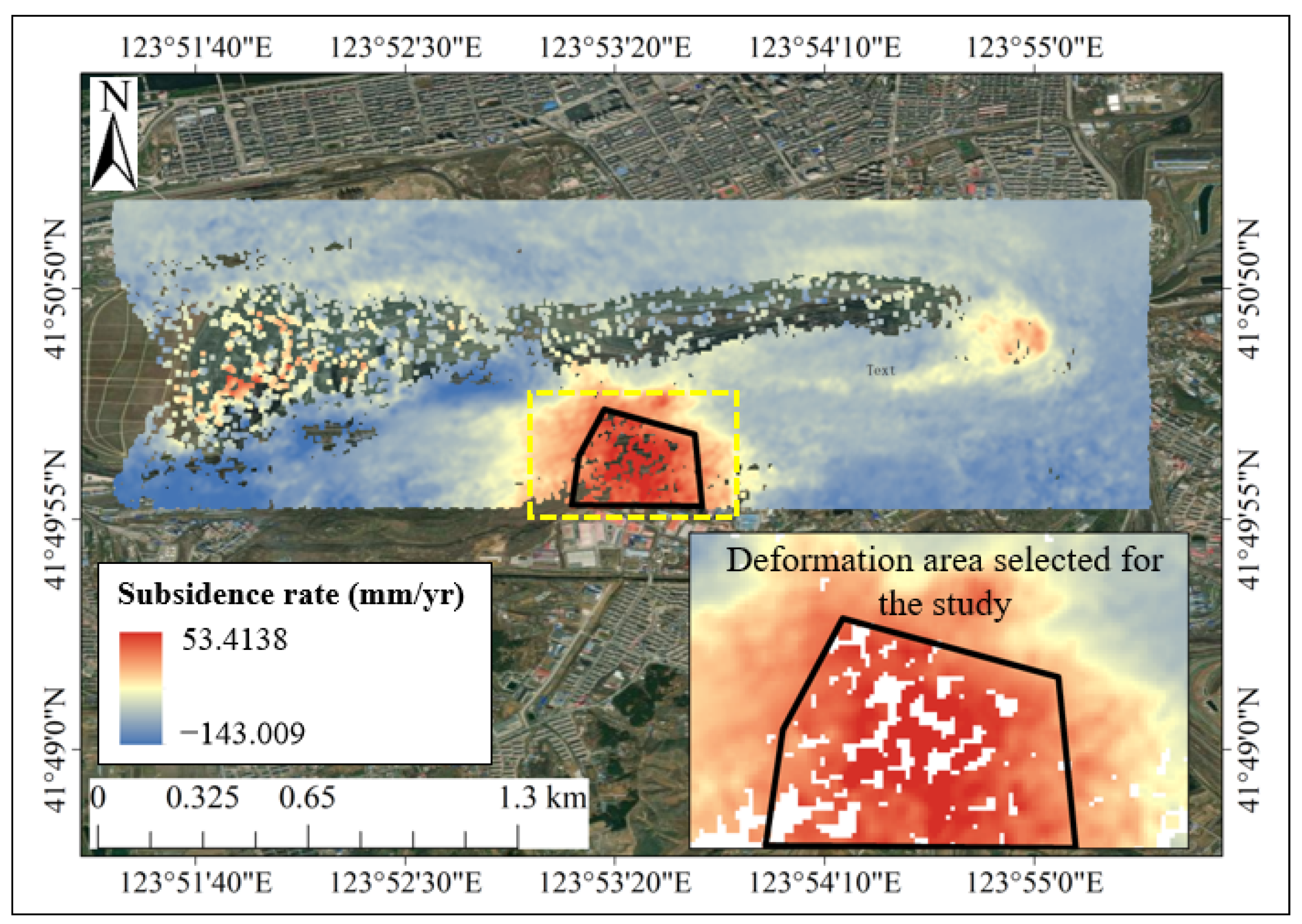
To meet the model requirements, the raster subsidence field was vectorized to extract high-coherence PS points. The initial PS point cloud, however, often contained noise and outliers caused by spatiotemporal decorrelation and atmospheric delays, while raster-to-vector conversion could introduce spatial sampling artifacts. To ensure reliable modeling, a rigorous data optimization procedure was applied. The vectorized PS points were first screened to remove low-coherence or anomalous points. Subsequently, a core region exhibiting strong deformation signals and spatial continuity was selected as the final dataset (Figure 12). This approach focused the analysis on the primary subsidence bowl, substantially improving the signal-to-noise ratio (SNR) and ensuring the dataset reliably represents the key deformation dynamics of the region.

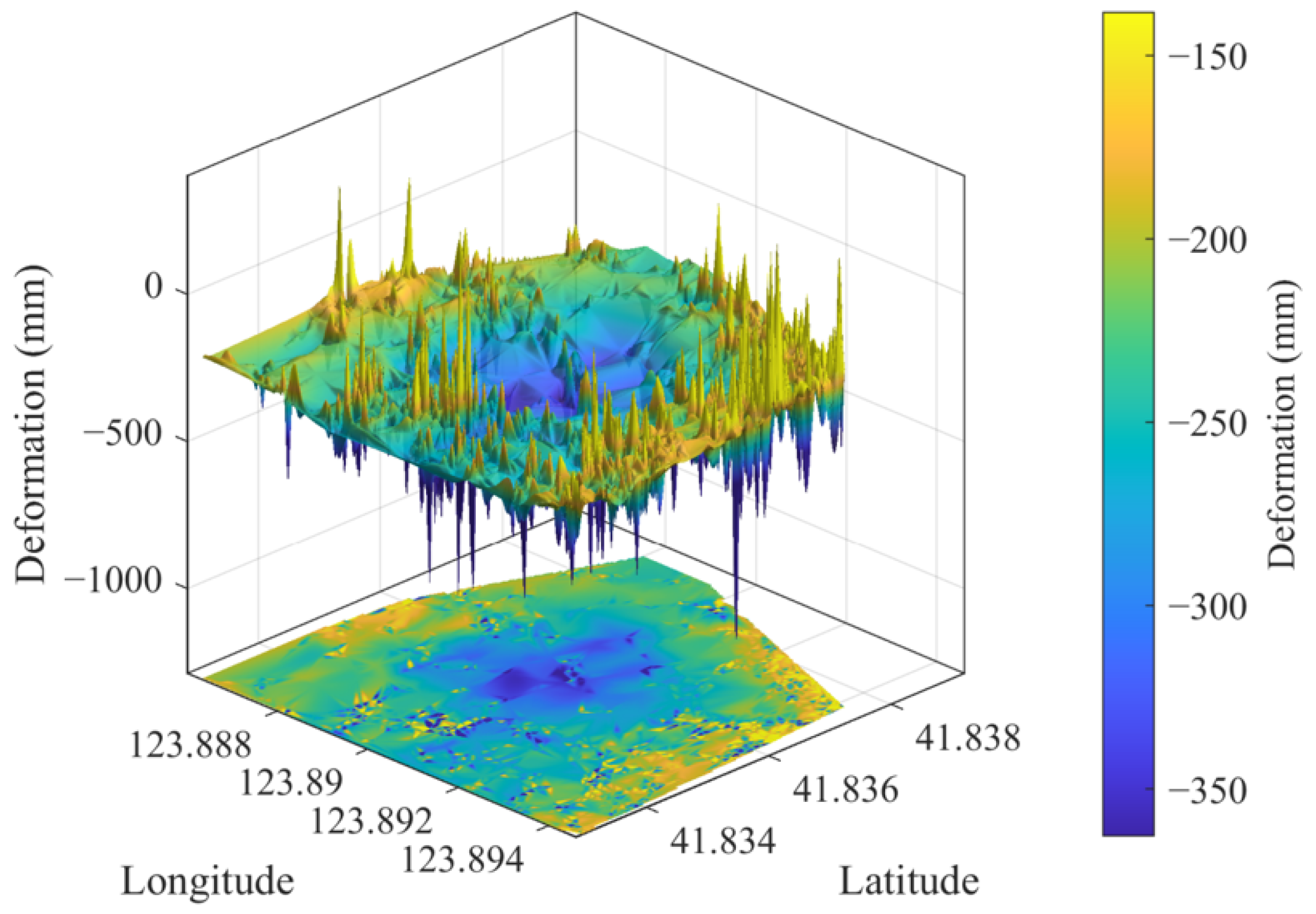
To further interpret the deformation characteristics of the selected core region, a three-dimensional (3D) deformation field was constructed (Figure 13). In this representation, the cumulative subsidence (mm) at each PS point is assigned as the elevation value (Z-axis) and projected onto its geographic coordinates (X–Y plane). This 3D visualization clearly illustrates the geometric morphology of the subsidence bowl, including the location of the maximum subsidence center and the spatial pattern of deformation gradients. The transition from 2D spatial filtering to 3D morphological analysis enhances understanding of the field’s heterogeneity and provides essential physical and geometric constraints for parameterizing and validating the subsequent prediction model.

Following the acquisition of high-quality PS point time series from the core deformation region, the data were subsequently converted into a supervised format suitable for deep learning training. A sliding-window method was applied to reconstruct each continuous PS time series into independent input–output sample pairs. For each PS point, a sequence of 65 consecutive time steps (infer_seq_length) was defined as the input features (X), capturing the recent subsidence evolution, while the subsequent 5 time steps (forecast_steps) served as the prediction labels (y).

To rigorously evaluate the model’s generalization capability for unknown future deformation and avoid data leakage (i.e., the “time travel” problem common in random shuffling), a strict chronological dataset splitting strategy was implemented. For every monitoring point, the sliding windows were divided strictly along the time axis into training, validation, and test sets. The earlier temporal sequences were used exclusively for model training, the intermediate sequences were allocated for validation, and the latest temporal sequences (representing the final five deformation periods) were reserved entirely as an unseen test set. Furthermore, Min–Max Scaling was applied to map both features and labels to a consistent numerical range, which improves the convergence efficiency of gradient-based training. Crucially, the normalization scalers were fitted solely on the training set and then applied to transform the validation and test sets. This strict separation ensures that adjacent overlapping sliding windows are never mixed across datasets, meaning no future information is inadvertently introduced during the preprocessing phase, thereby guaranteeing that the model performs genuine out-of-sample forecasting.

4.2. CL-TSF Hybrid Model Architecture

The proposed CL-TSF model follows a cascaded “feature extraction–sequence modeling–prediction” architecture. As shown in Figure 14a, it comprises three primary modules: a convolutional feature extraction module, a sequential modeling module, and a prediction module. The convolutional module functions as an encoder, converting raw one-dimensional inputs into abstract, information-rich features. The sequential modeling module serves as the core predictor, capturing long-term temporal dependencies through a stacked LSTM network. The prediction module then uses a fully connected layer to map the learned temporal features to multi-step forecast outputs. The detailed processing workflow for a single time step is shown in Figure 14b, illustrating how CNN-extracted features drive the state evolution of the LSTM cell.

(1) Convolutional Feature Extraction Module. The encoder transforms the original one-dimensional time-series input (length 65) into a shorter, feature-enhanced representation through two stages of convolutional downsampling (Figure 14c).

• First convolutional block. The input sequence is first processed by a Conv1D layer with 32 filters (kernel size = 3) to capture local patterns and short-term variations. Batch Normalization is then applied to stabilize activations and improve convergence, followed by MaxPooling (stride = 2), which reduces the sequence length from 65 to 33 while retaining salient features.
• Second convolutional block. The output is further refined by a second Conv1D layer with 16 filters (kernel size = 3), again followed by Batch Normalization and MaxPooling. This block produces a condensed feature sequence of length 17 with 16 channels, representing an abstract and information-dense encoding of the original input.

Through this hierarchical design, the encoder efficiently extracts key temporal features, reduces sequence length, mitigates computational load for the subsequent LSTM module, and enhances robustness to minor temporal shifts.

(2) Sequential Modeling Module. Serving as the key link between feature extraction and final prediction, the sequential modeling module is designed to capture complex temporal dynamics and long-term dependencies within the encoded feature sequences. As shown in Figure 14a, an LSTM architecture is employed to progressively aggregate and refine temporal information through cascaded nonlinear transformations.

• Temporal feature retention and high-dimensional encoding. The first LSTM layer contains 32 hidden units and operates in a sequence-to-sequence mode. It projects the CNN-extracted features into a higher-dimensional latent space while preserving the temporal structure of the sequence, thereby retaining the evolving dynamics at each time step and providing a solid basis for deeper temporal abstraction.
• Deep semantic compression and global representation. The second LSTM layer, with 16 hidden units, functions as a temporal information aggregator in a many-to-one configuration, outputting only the final hidden state. Through its internal gating mechanism, this layer integrates information over the entire sequence, yielding a compact representation that encapsulates the global temporal context of the subsidence process.
• Stochastic dropout regularization. To enhance generalization and suppress overfitting, a dropout layer with a rate of 0.2 is applied after each LSTM layer. This stochastic regularization strategy effectively mitigates overfitting during the training phase. Furthermore, to evaluate the reliability of the forecasting results in real-world early warning scenarios, this study introduces the Monte Carlo (MC) Dropout technique for uncertainty quantification. During the inference phase, the dropout layers in the sequential modeling module are kept active. By performing 100 independent stochastic forward passes for each test sample, the model generates a predictive distribution. The mean of these predictions serves as the final point estimate, while the 95% confidence interval is derived from the standard deviation, providing a statistically bounded error range for future deformation.

(3) Prediction Module. As the terminal regression component of the CL-TSF architecture, the prediction module is responsible for transforming the high-level abstract features produced by the sequential modeling module into physically meaningful predictive values.

• Linear mapping and multi-step forecasting. This module is implemented as a fully connected layer that serves as the output interface of the network. It receives the 16-dimensional final hidden-state vector from the LSTM layers and projects the learned latent features into the target observation space through a linear weighted transformation with bias. The output layer contains five neurons, corresponding to the predicted land-subsidence values for the subsequent five time steps, thereby completing the transformation from high-dimensional feature representations to quantitative multi-step time-series forecasts.

4.3. Model Compilation and Training Strategy

Once the model architecture had been established, its compilation and training parameters were configured to ensure that the nonlinear mapping from historical to future subsidence sequences could be learned through iterative optimization. The Adam optimizer was selected with an initial learning rate of 0.001. Owing to its computational efficiency, low memory demand, and adaptive adjustment of parameter-specific learning rates, excellent convergence performance is typically achieved when Adam is applied in deep learning tasks. The loss function was defined as Mean Squared Error (MSE) [50], which is computed as the average squared difference between predicted and observed values. Its sensitivity to large errors is considered particularly beneficial for enabling substantial prediction deviations to be rapidly reduced during the early stages of training.

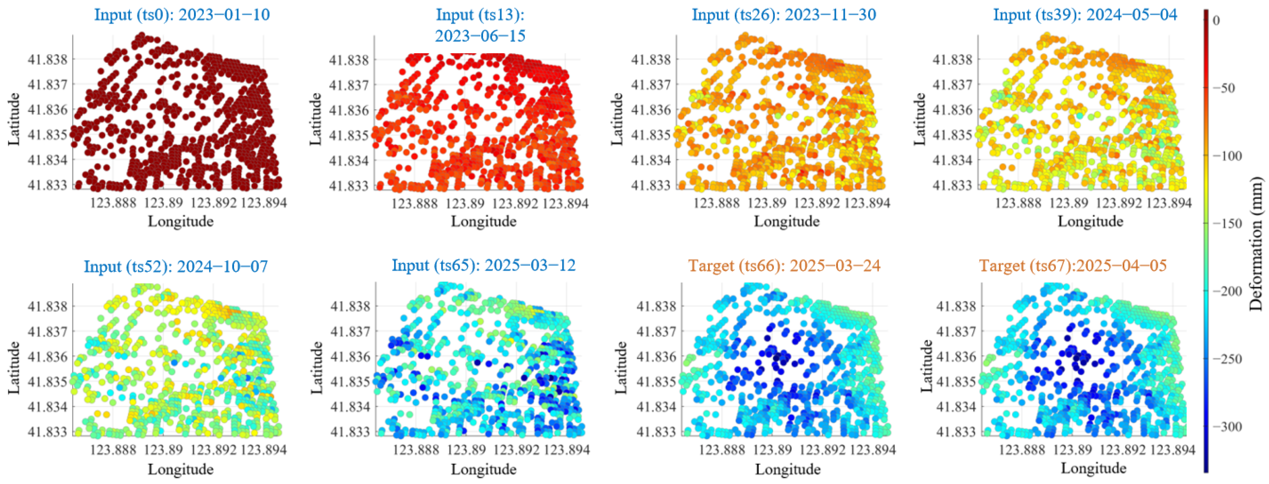
To illustrate the model’s learning task, Figure 15 presents the spatial deformation maps of a representative training sample across multiple time steps. The first six subplots (“Input”) visualize part of the input sequence and depict the temporal evolution of the surface deformation field, with the colormap transitioning from dark red (early stage, ts0) to cyan (late stage, ts65). This captures the dynamic information encoded in the 65-step input sequence. The last two subplots (“Target”) show the corresponding ground-truth deformation fields at ts66 and ts67, which constitute the prediction targets. During training, the model is required to extract the spatiotemporal features embedded in the “Input” and generate predictions that closely approximate the “Target” both numerically and spatially.

Guided by this objective, the model was designed to be trained for a maximum of 100 epochs with a batch size of 64. To effectively mitigate the risk of overfitting during the training process, an Early Stopping mechanism was incorporated. The model continuously monitored the validation loss (val_loss) at the end of each epoch. If the validation loss failed to improve for 15 consecutive epochs, the training process was automatically halted, and the model weights from the epoch with the lowest validation loss were restored. This approach provides a key measure of generalization performance and an automated corrective measure against overfitting. Furthermore, standard k-fold cross-validation was explicitly avoided in this study, as it inherently disrupts the strict temporal order of the time-series data and would reintroduce the risk of data leakage.

4.4. Evaluation of Forecasting Performance

To quantitatively evaluate the forecasting performance of the CL-TSF model for surface subsidence time series, three commonly used regression metrics were adopted: Root Mean Square Error (RMSE), Mean Absolute Error (MAE), and Mean Absolute Percentage Error (MAPE). Together, these indices provide a comprehensive assessment of predictive accuracy from different statistical perspectives.

$$\mathrm{RMSE}=\sqrt{{\displaystyle \frac{1}{N}}{\displaystyle \sum _{i=1}^N{(Y_i-y_i)}^2}}$$

(2)

$$\mathrm{MAE}={\displaystyle \frac{{\displaystyle \sum _{i=1}^N|}{Y}_i-y_i|}{N}}$$

(3)

$$\mathrm{MAPE}={\displaystyle \frac{1}{N}}{\displaystyle \sum _{i=1}^N\frac{|Y_i-y_i|}{\left|y_i\right|}}\times 100\%$$

(4)

In these equations, N denotes the total number of prediction samples; Y_i is the predicted value for the i-th sample; and y_i is the corresponding SBAS-derived ground truth.

5. Surface Subsidence Forecasting with the CL-TSF Model

5.1. Model Performance Comparison

To assess the predictive performance of the proposed CL-TSF model, its test-set outputs were compared with ground-truth labels following the previously established framework. Three models were included in the evaluation:

(1)

CNN: Used as a baseline emphasizing local temporal feature extraction. To ensure a fair comparison, its network complexity was configured to match the convolutional module of the CL-TSF model. It comprises two stacked Conv1D layers (with 32 and 16 filters, respectively, and a kernel size of 3), each followed by Batch Normalization and MaxPooling, and culminates in a fully connected dense layer.

(2)

LSTM: A second baseline designed to capture long-range temporal dependencies. Similarly, its structure was aligned with the sequential module of the CL-TSF model, consisting of two stacked LSTM layers (with 32 and 16 hidden units, respectively), with a dropout rate of 0.2 applied after each layer to prevent overfitting, followed by a fully connected dense layer.

(3)

Proposed CL-TSF hybrid model: Integrates the complementary strengths of CNNs and LSTMs—local feature extraction and long-term dependency modeling—to enhance overall prediction accuracy. To guarantee an equitable and unbiased comparison, all three models were strictly subjected to identical data preprocessing, sliding-window configurations (65 input steps and 5 output forecast steps), and unified training strategies. Specifically, all models were trained using the Adam optimizer with an initial learning rate of 0.001, a batch size of 64, and the Mean Squared Error (MSE) loss function over 100 epochs. Furthermore, to ensure fairness and objectivity, all models were trained and evaluated under a unified experimental protocol using the strictly chronologically split dataset described in Section 4.1. Because the test set comprises purely future time steps that the models have never encountered during training, this evaluation authentically reflects each model’s capacity for genuine temporal extrapolation. Although model training was performed on normalized data to promote stable convergence, performance evaluation was carried out on the original data scale by applying an inverse transformation to the predictions before comparison with the ground-truth values. This standardized workflow ensures that the reported MAE, MAPE, and RMSE values faithfully reflect each model’s predictive accuracy in physical units.

After repeated trials over the full sample set, the comparative performance of the three models is summarized in

Table 1. Overall performance comparison of different models on the test dataset.

Index	CL-TSF	LSTM	CNN
RMSE	5.260	6.634	11.366
MAE	4.723	5.863	10.289
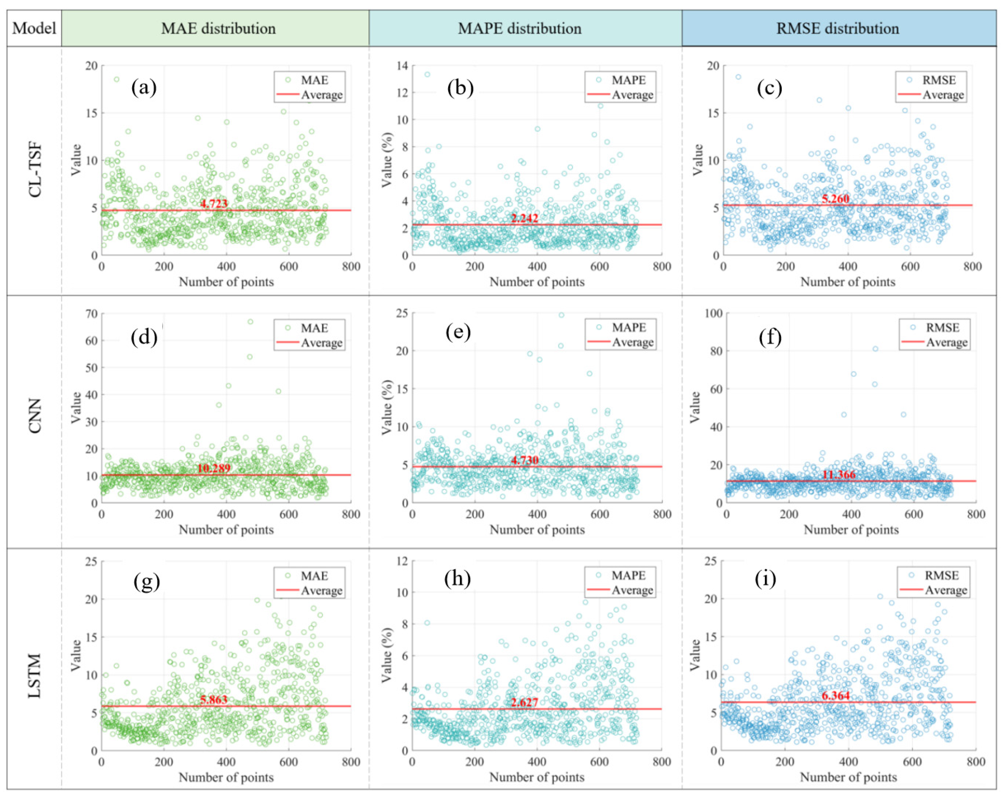
MAPE	2.24%	2.63%	4.73%

. To further illustrate their error characteristics, the corresponding MAE, MAPE, and RMSE distributions are shown as scatter plots in Figure 16. As summarized in Table 1, the CL-TSF model outperforms both benchmark models across all evaluation metrics. Compared with the next-best model, LSTM, CL-TSF achieves reductions of 20.7% in RMSE, 19.4% in MAE, and 14.8% in MAPE. This quantitative advantage is corroborated by the error distributions shown in Figure 16, which presents scatter plots for the CL-TSF model (Figure 16a–c), CNN (Figure 16d–f), and LSTM (Figure 16g–i). A row-by-row comparison shows that CL-TSF errors are characterized by the lowest mean and the tightest clustering for all metrics. In contrast, the CNN model exhibits the widest dispersion, the highest mean error, and numerous large outliers, indicating substantial instability. The LSTM model displays intermediate performance, with a more concentrated error distribution than CNN but a wider scatter and higher mean than CL-TSF. These results confirm that the CL-TSF model not only achieves superior average accuracy but also provides the highest stability and reliability.

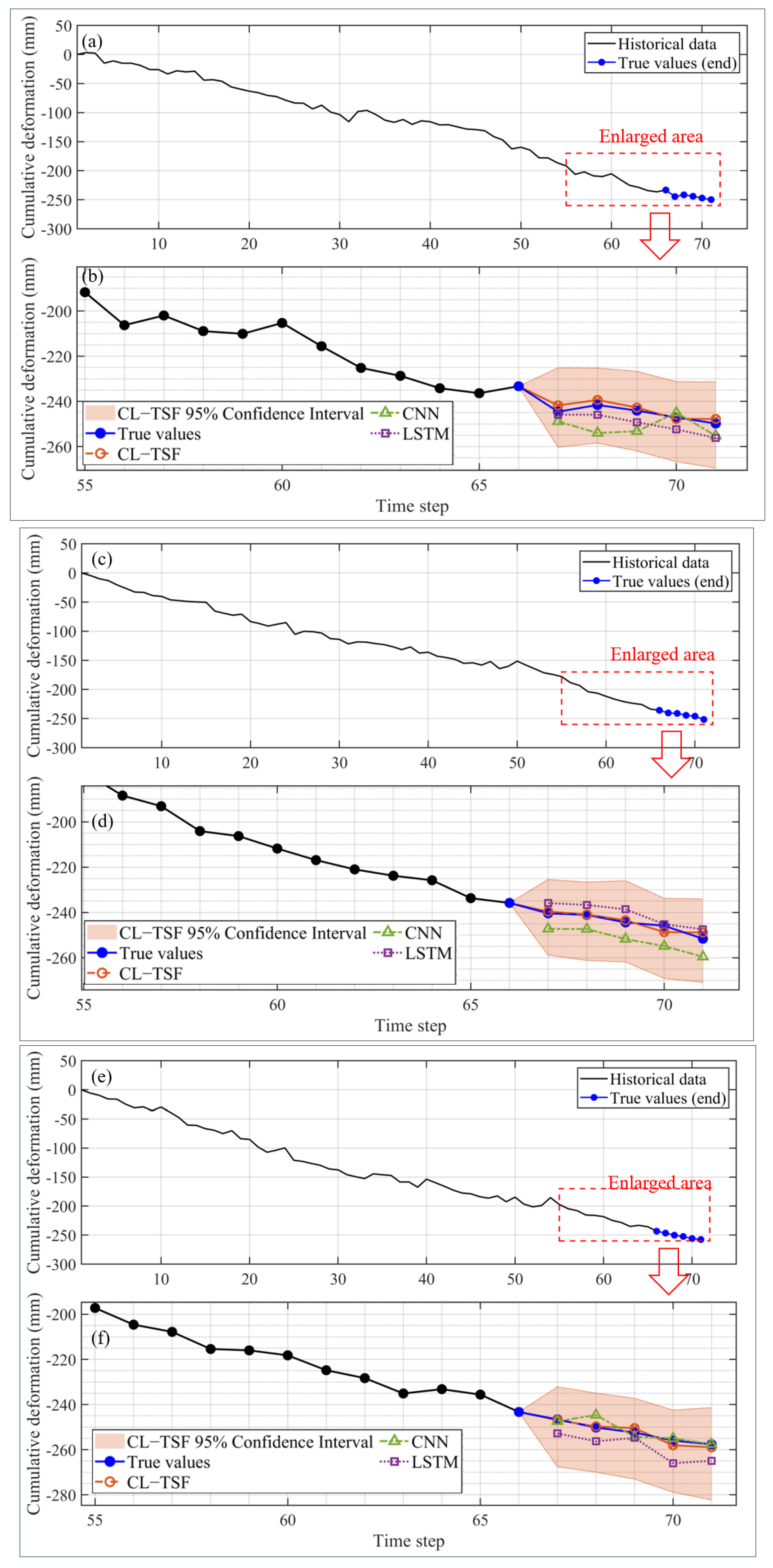
To examine the predictive behavior of different models at the micro scale, three representative monitoring points were selected from the 720-sample test set, located at the beginning (Row 11), middle (Row 421), and end (Row 691) of the dataset. This selection strategy was designed to assess model generalization and performance consistency across different sample positions. The corresponding multi-step prediction results are shown in Figure 17, and the associated quantitative error metrics are summarized in

Table 2. Error statistics of prediction results at representative monitoring points (Figure 17).

Monitoring Point	Model	RMSE	MAE	MAPE
11	CL-TSF	1.9466	1.7966	0.73%
	CNN	7.6092	6.6678	2.73%
	LSTM	4.8079	4.4890	1.83%
421	CL-TSF	1.8127	1.4732	0.60%
	CNN	7.5336	7.4755	3.05%
	LSTM	4.2663	3.9098	1.60%
691	CL-TSF	1.4279	1.2364	0.49%
	CNN	2.6852	1.8647	0.74%
	LSTM	6.8534	6.3972	2.53%

. Based on the combined analysis of Figure 17 and Table 2, the following observations can be made.

(1)

Adaptation to nonlinear dynamics (Monitoring point 11; Figure 17a−b). This monitoring point exhibits pronounced short-term nonlinear fluctuations prior to the prediction horizon. Under such conditions, the CL-TSF model achieves the lowest MAPE (0.73%), demonstrating strong robustness and superior capability in capturing complex temporal dynamics.

(2)

Performance consistency (Monitoring point 421; Figure 17c−d). Located near the center of the dataset, monitoring point 421 is characterized by a relatively stable downward deformation trend. The CL-TSF model again yields the lowest MAPE (0.60%), while the CNN and LSTM models produce MAPEs of 3.05% and 1.60%, respectively. This result indicates that the performance advantage of the CL-TSF model is stable and not dependent on specific sample locations.

(3)

Performance under stable trends (Monitoring point 691; Figure 17e–f). This monitoring point exhibits an approximately linear and steady subsidence trend. Although all models are able to capture the overall deformation tendency under such simplified conditions, notable differences in prediction accuracy are observed. The CL-TSF prediction closely matches the ground truth, achieving a MAPE of only 0.49%, which is substantially lower than those of the CNN (0.74%) and LSTM (2.53%). Notably, the CNN outperforms the LSTM in this case, suggesting that short-term local features may be more informative than long-term dependencies for this specific temporal segment.

As shown in Figure 17, the 95% confidence intervals (shaded regions) generated by the MC Dropout method are incorporated into the multi-step predictions. The relatively narrow confidence bands across monitoring points 11, 421, and 691 indicate that the CL-TSF model maintains high predictive certainty, even when extrapolating future trends. This uncertainty quantification is highly significant for engineering practices; it transitions the model from providing mere deterministic values to offering a statistically bounded risk range, thereby enabling more reliable threshold-based early warning decisions in open-pit mines.

By integrating macroscopic statistical results with microscopic case analyses, the superior performance of the CL-TSF model can be attributed to the synergistic design of its hybrid architecture. The CNN module efficiently extracts discriminative local features, the importance of which is evident from the results at monitoring point 691. These abstracted representations are subsequently fed into the LSTM module, which effectively captures their temporal evolution. This “feature extraction–sequential modeling” paradigm enables the CL-TSF model to better characterize the underlying complex deformation dynamics, thereby outperforming standalone CNN or LSTM models in terms of both prediction accuracy and stability. Consequently, the proposed CL-TSF model provides more accurate and reliable deformation forecasts for the study area.

5.2. Subsidence Prediction Results of the CL-TSF Model

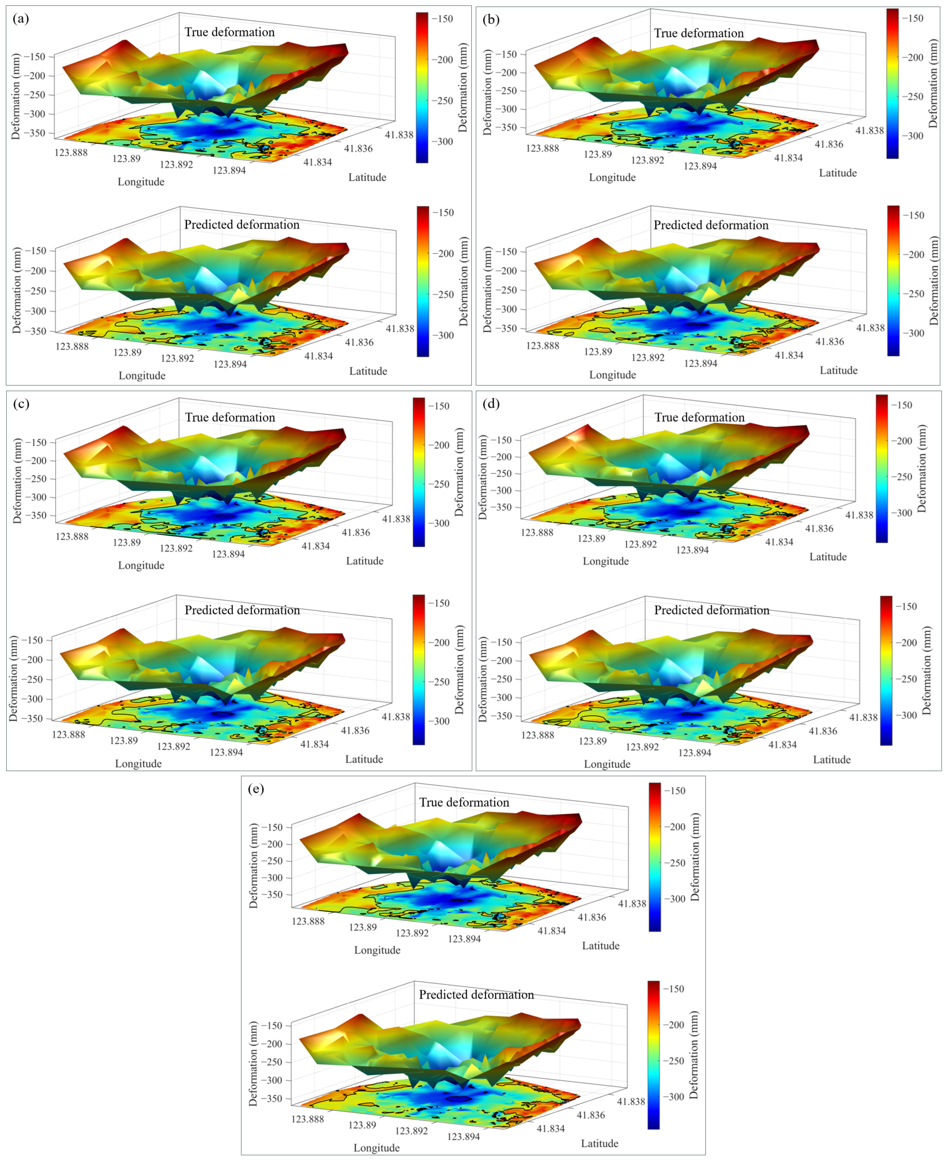
This section provides a comprehensive evaluation of the CL-TSF model’s performance in forecasting dynamic surface subsidence under the complex geological conditions of the Fushun West Open-pit Mine. A detailed comparison was conducted between the model predictions and SBAS-InSAR–derived ground-truth data across five consecutive periods (66–70). As shown in Figure 18, each subfigure presents paired 3D views in which the upper plot depicts the SBAS-InSAR–derived subsidence field and the lower plot shows the corresponding model prediction. A uniform colormap and scale were applied to both datasets at each time step to enable an objective, one-to-one comparison between color gradients and subsidence magnitude, allowing a clear visual assessment of the model’s predictive accuracy.

A sequential analysis of the prediction results is summarized as follows:

(1)

Initial prediction (Period 66; Figure 18a). The ground-truth subsidence field shows a well-defined primary subsidence bowl centered at 123.892–123.894°E and 41.834–41.836°N. The CL-TSF model reproduces this feature with high fidelity, accurately capturing its location, extent, and gradient, with subsidence deepening from roughly −160 mm at the margins to −320 mm at the center.

(2)

Stable evolution (Periods 67–68; Figure 18b,c). During periods 67 and 68, the observed subsidence evolves steadily, with a slight expansion of the bowl footprint while the maximum magnitude remains unchanged. The model maintains strong temporal coherence and continues to match the spatial morphology and magnitude of the observed fields.

(3)

Complex dynamics (Period 69; Figure 18d). Period 69 marks the appearance of a secondary subsidence zone in the southwestern sector. The model successfully captures this emerging feature, demonstrating its ability to track both the growth of existing subsidence and the development of new deformation patterns—reflecting the CNN’s strength in extracting localized spatial signatures.

(4)

Long-term forecast performance (Period 70; Figure 18e). By period 70, the true subsidence field exhibits increased complexity with multiple irregular sub-zones. Despite the greater predictive difficulty, the model continues to generalize well, accurately representing the ongoing evolution of the main bowl and providing reasonable approximations of the more intricate secondary features.

Overall, the performance across the entire prediction sequence indicates that the CL-TSF model effectively captures the multi-stage subsidence process—from steady progression to complex spatial reorganization. Its hybrid architecture leverages CNN-based spatial feature extraction and LSTM-based temporal dependency modeling, enabling it to learn the nonlinear spatiotemporal deformation dynamics and deliver high-fidelity predictions that reflect both broad-scale trends and fine-scale variations.

5.3. Prediction Error Analysis

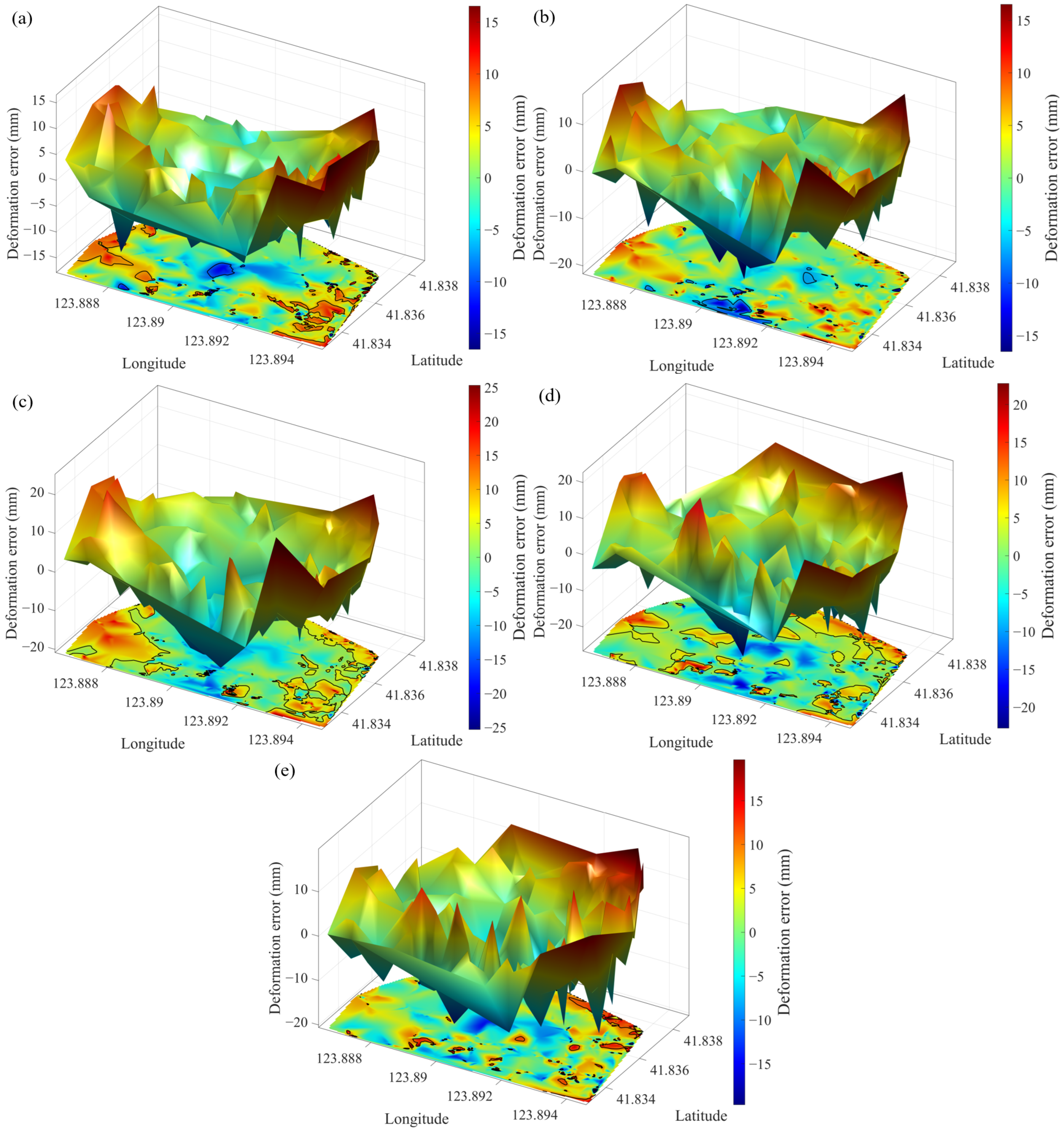
To quantitatively validate the aforementioned visual comparisons, the prediction error—defined as the difference between the true and predicted subsidence values—was calculated for each monitoring period. The spatial distribution of these errors is shown in Figure 19. Positive values (red) indicate under-prediction, where the predicted subsidence is smaller than the SBAS-InSAR measurements, while negative values (blue) represent over-prediction, where the predicted magnitude exceeds the true deformation.

A temporal evolution analysis of the prediction error is summarized as follows:

(1)

Initial prediction error (Period 66; Figure 19a). At the start of the forecast, the error is spatially localized and small across the study area. Most values fall within ±10 mm, with slightly larger errors (up to ±15 mm) appearing only along the steep deformation gradients at the bowl margins. This indicates high predictive fidelity even in zones with strong spatial variability.

(2)

Error stability (Periods 67–68; Figure 19b,c). The error patterns in periods 67 and 68 remain highly consistent with those in period 66, confirming the model’s predictive stability. Large areas show near-zero error, indicating an excellent match between predicted and observed values. Importantly, peak errors do not increase over time; the maximum absolute error stays at roughly 15 mm, demonstrating effective suppression of short-term error accumulation.

(3)

Long-sequence error control (Periods 69–70; Figure 19d,e). Toward the end of the forecast horizon, the model continues to maintain tight error control. In period 70, despite slightly increased fluctuations, more than 90% of the area retains absolute errors within 20 mm. The maximum positive error (~+20 mm) occurs along the northeastern boundary, while the maximum negative error (~−20 mm) appears near the subsidence center. Given the complex deformation patterns of the mine and the inherent noise in InSAR data, this level of accuracy reflects excellent long-term predictive performance and surpasses that of many conventional time-series models.

In conclusion, the five-period analysis demonstrates the strong predictive capability of the CL-TSF model for surface subsidence at the Fushun West Open-pit Mine. The model accurately reproduces both the spatial pattern and magnitude of the deformation field, effectively tracks its temporal evolution, and maintains very low cumulative errors over extended forecast horizons. Its high accuracy and stability highlight its potential to support real-time deformation monitoring, geohazard risk assessment, and scientific mining management.

5.4. Remaining Challenges

The primary contribution of this study is the development and validation of the CL-TSF deep learning model, which synergistically fuses spatiotemporal features to achieve accurate dynamic subsidence forecasting in an operational mining environment. The model integrates a CNN module to extract local spatial features of the subsidence field and an LSTM module to capture their temporal evolution, thereby overcoming key limitations of traditional approaches in modeling complex nonlinear deformation processes. Beyond providing valuable insights into the subsidence mechanisms of the Fushun West Open-pit Mine, the high-fidelity forecasts generated by the CL-TSF model offer a practical and robust framework for dynamic early warning and geohazard risk assessment in mining areas.

While this study provides promising results, it also acknowledges certain limitations regarding causal analysis. Surface subsidence in mining areas is a complex process governed by coupled hydro-mechanical interactions. Ideally, identifying strict causality requires isolating confounding variables such as precise underground mining intensity and dynamic groundwater level fluctuations. However, as the Fushun West Open-pit Mine is a strictly controlled industrial site, high-resolution operational data and internal hydrological records are classified as confidential. Consequently, this study primarily relies on statistical correlation and time-lag analysis to infer the triggering role of rainfall. Future work, upon the declassification of or authorized access to such multi-source engineering data, could integrate physics-based numerical modeling to decouple these confounding variables and achieve a more rigorous causal inference. Moreover, applying the validated CL-TSF model to mining sites with varying geological and operational settings is essential for evaluating its generalization and transferability [51,52]. Assessing the model’s performance over longer forecast horizons (e.g., 6–12 months) and examining error-accumulation behavior and mitigation strategies also represent important research avenues [53]. Overall, the findings of this study hold substantial theoretical value and offer broad potential for practical application.

5.5. Practical Implementation and Generalization

Regarding model generalization, while this study validates the CL-TSF model within the specific hydrogeological context of the Fushun West Open-pit Mine, its underlying architecture possesses strong transferability. For future applications in other mining sites with varying geological settings, a Transfer Learning (TL) strategy is recommended [54,55]. The pre-trained weights from the current CNN-LSTM network can serve as a foundational model. When migrating to a new site, only a small amount of local InSAR time-series data and meteorological records would be required to fine-tune the fully connected layers. This approach significantly reduces the data dependency and training costs for new mining areas, enabling rapid deployment.

Furthermore, to translate the predictive outputs of the CL-TSF model into actionable dynamic early warning operations, a multi-tier threshold system integrated with a Digital Twin framework is conceptualized [56]. The early warning thresholds should be dynamically defined based on industry standards and local geological tolerance. For instance, a three-tier system can be established based on the predicted deformation rates: Level III (Yellow, attention required) for rates exceeding 2 mm/day; Level II (Orange, restricted access) for rates exceeding 5 mm/day; and Level I (Red, immediate evacuation) for sudden acceleration indicating potential landslide failure [57]. In practical implementation, the InSAR-derived long-term predictions from the CL-TSF model should be fused with real-time, high-frequency IoT sensors (e.g., GNSS, crack meters, and piezometers) [58]. The CL-TSF model provides the macro-scale spatial trend and mid-to-long-term forecasting, while real-time sensors provide micro-scale validation, together forming a robust, closed-loop geohazard early warning system.

6. Conclusions

This study addresses safety risks associated with slow-onset, mining-induced geohazards by integrating time-series InSAR monitoring with deep learning–based prediction for the Fushun West Open-pit Mine. The spatiotemporal evolution and driving mechanisms of surface subsidence were systematically analyzed, and the main conclusions are as follows:

(1)

Time-series InSAR analysis of 70 Sentinel-1A images acquired between January 2023 and May 2025 identified a large-scale, continuously evolving subsidence bowl within the mining area. The maximum subsidence rate reached 143.00 mm/yr, with a cumulative displacement of −337.89 mm.

(2)

Rainfall was identified as the dominant external control on surface deformation. Comparative analysis of InSAR-derived deformation and monthly precipitation records revealed strong seasonal coherence, with Pearson correlation coefficients of up to 0.71 at key monitoring points. Surface subsidence exhibits pronounced lagged and cumulative responses, characterized by a one- to two-month delay following major rainfall events and sustained modulation by antecedent hydrological conditions.

(3)

The influence of regional seismic activity on subsidence was quantitatively evaluated using the SESA framework, in combination with linear regression and Grey Relational Analysis. The results indicate no meaningful linear relationship (R² < 0.014) between peak ground motion parameters (PGA and PGV) and short-term post-seismic subsidence. Although PGV exhibited the highest relative correlation, its absolute influence was negligible and indistinguishable from the background deformation signal, indicating that regional seismicity acted only as a minor perturbation during the study period.

(4)

To accurately predict the complex subsidence process, a CL-TSF hybrid model was developed. Comparative evaluations demonstrate that the proposed model significantly outperforms conventional CNN and LSTM approaches, achieving a MAPE of 2.24% and an RMSE of 5.260. Its accuracy, stability, and robustness were further validated through reliable multi-step prediction and 95% confidence interval estimation of the final five deformation periods, supported by three-dimensional visualization and detailed error analysis.

Overall, this study establishes an integrated framework for the monitoring, interpretation, and prediction of mining-induced surface subsidence, providing robust technical support for dynamic early warning and risk mitigation in open-pit mining environments and analogous geological settings.