Article

Monitoring Coastal Geomorphic Change and Sediment Transport Using Kite Aerial Photography (KAP) and Structure-from-Motion (SfM) Photogrammetry

by
Julia Sarachik-Epstein
,
Jerry D. Davis
* and
Andrew J. Oliphant
School of the Environment, San Francisco State University, San Francisco, CA 94132, USA
*
Author to whom correspondence should be addressed.
Remote Sens. 2026, 18(17), 2998; https://doi.org/10.3390/rs18172998
Submission received: 26 May 2026 / Revised: 16 August 2026 / Accepted: 19 August 2026 / Published: 3 September 2026

Highlights

What are the main findings?
  • Kite aerial photography (KAP) with spatially variable error modeling using a fuzzy inference system was effective for assessing geomorphic change in dune systems, with mean error < 5 cm.
  • KAP-based observations of sand accumulation over time scaled closely with wind-driven estimates of sediment transport for the same periods, with morphological change providing a measure of captured accumulated sediment representing between 50 and 80% (R2 = 0.98) of wind modeled estimates from cross-sections aligned with the prevailing wind.
What are the implications of the main findings?
  • KAP is a reliable survey method for the monitoring and analysis of geomorphic change when paired with RTK or NTRIP GNSS, robust spatially variable error modeling, and accuracy assessments.
  • KAP-derived DEM of Difference (DoD) allows for assessing seasonal changes in sediment mass transport and comparison with wind model-derived estimates.

Abstract

Coastal areas are particularly suitable study sites for kite aerial photography (KAP) surveys because of consistent wind and open space. This study uses KAP surveys conducted in January, March, June, August, and October 2025, combined with Structure from Motion photogrammetry and spatially variable error modeling for DEM of Difference (DoD) thresholding to monitor a dune revegetation project at Ocean Beach in San Francisco. Two independent ground surveys were conducted in June and October to compare measured elevation data with KAP-derived elevation. A fuzzy inference system was used to model spatially variable error for uncertainty thresholding with a 95% confidence interval based on point cloud density and surface roughness. The elevation models (raw and thresholded) were then analyzed through geomorphic change detection to assess volumetric change over time. DoD estimates from the four sampling periods between flights were used to derive mass transport rates (120.09, 415.04, 270.86, and 102.22 kg m−1 d−1, respectively) from cross-sections aligned with estimated wind directions, with results similar to wind model estimates from the same time periods, ranging from 50 to 80% (R2 = 0.98) of the latter. This method holds promise for better connecting geomorphic to atmospheric research methods, especially important when pursuing process-based restoration.

1. Introduction

Kite aerial photography (KAP) can be a low-cost option for high-spatial-resolution, low-altitude remote sensing [1,2]. Coastal dunes and intertidal landscapes are particularly suitable study areas for KAP-based surveys because of consistent wind and open space [3,4,5]. This study uses KAP as a method for monitoring a dune revegetation project at Ocean Beach in San Francisco at a study site experiencing persistent erosion and applies spatially variable errors measured from KAP-derived elevation data to develop a more reliable surface raster of sand deposition above the uncertainty threshold that may have resulted from the restoration project. From this surface, we estimated downwind sand transport rates to compare with wind model-derived rates for sediment transport. Our methods contribute to the call for research on understanding mass transfer in landscape elements at the local scale [6], compared with nonlocal transfer estimates driven by processes in the atmospheric boundary layer.

1.1. KAP and Other SfM Methods for Environmental Monitoring

Remote sensing from satellite data offers large-area coverage, multispectral imaging, and availability for broad spatial coverage and long-term environmental change monitoring. Satellite imagery is becoming available in increasingly finer resolution and has been used for monitoring coastal dunes in shoreline progradation/erosion studies [7]. However, there remain limitations in achieving the spatial resolution needed to generate digital elevation models sufficiently precise to assess short-term, local geomorphic change at the scale of coastal dune features [7,8,9,10]. For the assessment of morphological changes, aside from a few studies, researchers commonly rely on terrestrial or UAV-based monitoring approaches [11,12,13,14,15].
Unoccupied aerial systems or unoccupied aerial vehicles (UAVs) typically refer to drones, but also include balloons, blimps, and kites. The rapid data collection and processing capabilities make UASs an attractive survey method, especially when paired with other types of data [16]. Imagery and data gathered from these platforms can help to bridge the gap between in situ measurements and those collected by coarser-resolution satellite sensors [2].
Though drones have become the platform of choice for many researchers, there are myriad challenges with drones, including complex maintenance and operational requirements, cost, regulation, inability to operate in high winds, and potential wildlife disturbance [2,17]. In contrast, kites are low-cost, low-energy-use, operationally simple, legally uncomplicated, and less disturbing to sensitive wildlife [2,18]. KAP presents an alternative survey technique for low-disturbance studies where there may be sensitivity for vegetation, nesting birds, or mammals, or at visitor-heavy parks and beaches. There are many places, such as Ocean Beach, San Francisco, California, where kites can fly without much impact, but drones are not permitted or could have unintended impacts on wildlife.
For KAP-based surveying, researchers must consider materials (e.g., kite type, camera, rigging system), flight height and ground sampling distance, ground control points, and accuracy assessments. For the most part, studies that document UAS-SfM workflows for creating high-resolution digital elevation models are applicable to KAP [19,20,21]. For instance, ground control points (GCPs) are used to georeference the three-dimensional landscape models constructed from the collected imagery, and camera limitations due to weight constraints may make this more critical. Because high-accuracy GNSS is not as easily integrated with the lightweight devices used for KAP, kite-based surveys typically rely entirely on GCPs for location information.
Structure-from-Motion (SfM) photogrammetric methods use images acquired from multiple positions to construct 3D point clouds or digital elevation model (DEM) surfaces [19,21,22]. In contrast to traditional photogrammetry that employs very large frame negatives, images from most camera models can be used, with a high degree of overlap sometimes from non-nadir perspectives capturing the scene from many different viewpoints, making up for the much smaller sensors [19,20,21]. SfM data is often combined with LiDAR and terrestrial laser scanner point clouds [23,24,25] that provide better penetration to terrain surfaces through vegetation.
SfM from UAVs clearly provides advantages for geomorphic change detection at an appropriate scale for the equipment and research time available [26], and has been widely useful for assessing the effectiveness of landscape restoration such as riverscapes and ecogeomorphic features in meadows [6,20,27,28,29,30,31]. This relatively simple and low-cost technique for producing high-resolution topographic data mostly involves drones, but some studies may be well-suited to KAP surveying [20,21,32]. Though KAP surveys can be unpredictable, under optimal conditions, kites can allow for the required acquisition of overlapping photos from multiple viewpoints. Furthermore, while photogrammetric effectiveness at low cost and suitability for use in difficult terrains such as gullies and landslides have often been noted as advantages of SfM methods [20,29,33,34,35], particularly significant to KAP and for use in a popular recreation area is the suitability of lightweight snapshot cameras that can be easily raised by kites and do not present a significant hazard for people.
While accuracy assessments are of critical importance across all studies which use UAS-derived data, the inconsistencies in KAP surveying make testing for error and accuracy, and spatially variable error in particular, especially important. Assessment is commonly conducted by comparing KAP-SfM data products with outputs from other data sources such as terrestrial laser scanning and LiDAR [20,21,22,26] or from GNSS point observations [1,21]. Quantifying error allows the user to determine a minimum level of detection (minLoD) threshold by which geomorphic change can be measured, to filter out a level of error, either using a spatially consistent or spatially variable uncertainty threshold [36,37,38]. Multiple methods have been developed to assess the spatial variability of error, including using fuzzy inference systems that apply probabilistic thresholding, employing a specified confidence level [38]. We build on this work in the application of fuzzy logic to KAP survey techniques, and compare KAP-derived geomorphic change detection results with wind modeled rates to assess whether KAP-derived data can be used to accurately predict sediment transport.

1.2. Coastal Dunes

The application of this study is in mapping coastal sand dunes: Aeolian landforms that are present along many coasts, marking the transition from marine to terrestrial environments, are the most landward component of the sand-sharing system between the highly mobile beach and more stable dune. They develop where there is a supply of loose sand available to be transported by wind [39]. Primary factors that influence dune formation and morphology are wind, sand, and vegetation [39,40,41]. Coastal sand dunes are distinguished from other dunes mainly because of the presence of vegetation that affects coastal dune development by inhibiting the inland penetration of sand, depending largely on the height and density of plants [40,41,42,43,44,45,46].
Vegetation traps wind-blown sand and holds it in place, where it collects around the stems of plants specially adapted to grow upward through sand accumulation [40,45,46,47]. Vegetation disrupts the otherwise smooth surface, which slows down wind and consequently wind-blown sand, leading to deposition. It serves as a roughness element that slows the momentum transferred to the soil by the wind [48,49]. Dunes that are highly vegetated can be relatively stable landforms [50].
Climate and broader regional context also play a role in dune morphology because beaches in wet or humid tropics tend to experience less aeolian transport and less salt spray and are altogether more stable than beaches in temperate regions [51]. In San Francisco, this can mean more sediment transport in the summer: when the climate is driest and when onshore winds are stronger and more consistent.
Dunes can store and supply sand, and a strong dune ecosystem can reduce erosional impacts and sediment transport from waves, wind and storms [43,47,50]. Dunes provide ecosystem services and functions in coastal environments, including coastal protection from storms, filtering of pollutants, and generating biological productivity and diversity [47]. They are also niches for plants; refuge areas and habitat for insects, reptiles, birds and mammals, including for endangered species such as western snowy plovers; and recreational space for people [47]. Dunes are commonly an important part of shorebird migration paths, such as in San Francisco, where dunes are a critical corridor along the coastline [52].
Sand dunes in San Francisco originally ranked as one of the four most extensive complexes in California before urbanization, but very little of the once vast dune fields remains [42,52]. In California, much of the coastline has been filled, paved over, and cut off from natural sediment supply [42,52,53,54]. The protection of the dunes and sand management are particularly important in San Francisco because the dunes run alongside miles of critical infrastructure, including a highway, coastal armoring, and storm and wastewater infrastructure.
Where dunes have been destroyed, restoration and improvement strategies can involve rebuilding dunes where they have been eliminated, augmenting their space, or allowing natural processes to reform them into the landforms that naturally emerge, providing a diverse habitat with varied topography [47]. Dune building with vegetation, as is ongoing at the study site, is one method for restoration and uses vegetation to increase surface roughness and drag, which eventually slows wind speed and leads to sand deposition in plant species [40,45]. For a coastal dune to be stable (not growing or deflating), the dune must 1) be far enough from the shoreline to be unimpacted by wave erosion, 2) have complete vegetation cover so surface sand is not as exposed to wind, and 3) have no external source of sand for deposition [55].
Aeolian sand transport models using local wind observations can be helpful in relating observed dune changes to transport regimes over time. For example, Craig (2000) compared coastal dune slip face advance rates with transport predicted using local wind data [56] and Lamy et al. (2024) used the combination of modeling and observational approaches to examine the role of changing grain sizes on transportation rates [57]. There are many aeolian sand transport models based on boundary layer principles and the assumption that the transport rate is proportional to friction velocity to the third power. Though it has evolved over time, the first physics-based, laboratory- and field-tested, aeolian transport model in 1937 still performs well in recent model comparisons [40,58].

1.3. Research Objectives

This study assesses geomorphic changes in a dune and embankment area under restoration (using dune grass planting) through the collection of a succession of elevation surfaces at a coastal dune study site in San Francisco, California. Data were collected using kite aerial photography (KAP) as well as more traditional survey methods for ground truthing and accuracy assessments. The analysis of the KAP-derived data includes a spatially variable error analysis and geomorphic change detection of the elevation data.
Our research objectives are two-fold: (1) to test the feasibility and accuracy of kite aerial photography as a method for collecting high-resolution topographic data using a spatially variable error threshold for geomorphic change detection; and (2) to compare estimates of sand transport using KAP-based morphological DEM-differencing with micrometeorological wind-based estimates for understanding sediment transport. These objectives provide a better understanding of the key systems at play that should help to guide the long-term success of a process-based dune restoration project. Our method holds promise for better connecting geomorphic to atmospheric research methods, especially important in studying spatiotemporally dynamic systems such as coastal dunes.

2. Materials and Methods

2.1. Study Site

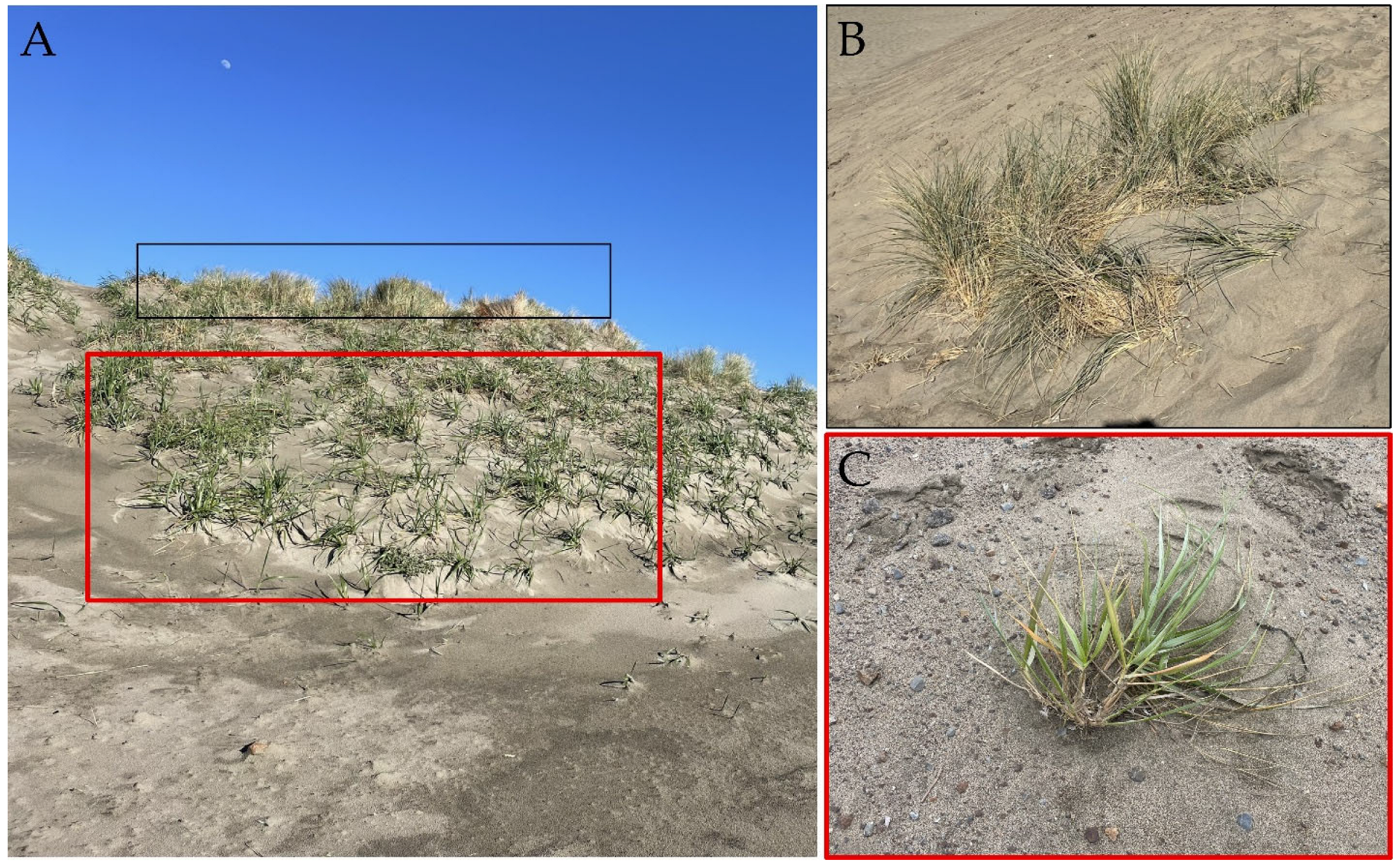
The study site is a roughly 1.5-hectare sand embankment area located at Ocean Beach in San Francisco, California. This is part of the unceded ancestral homeland and territory of the Ramaytush Ohlone, the original peoples of the San Francisco Peninsula. At the start of the study, the site was completely unvegetated and experiencing persistent erosion and sediment transport landward (eastward) due to a combination of strong onshore wind and a lack of vegetation to hold sand in place [52,59]. What began as a trail to the beach slowly destabilized and lost vegetation, leading to an enlarged blowout that eventually evolved into the unvegetated embankment that is present today (see Figure 1) [59]. A revegetation pilot project that aimed to slow eastward dune migration by planting beach wildrye (Leymus mollis), native beach grass, began in winter 2025, which initiated the start of this study [60,61].
This part of Ocean Beach features a wide beach, general trend of sand accretion, landward migration of foredunes, and generally onshore wind. San Francisco is a unique environment, where the offshore bathymetry and shoreline to the North and South are irregular and impact waves and littoral sand transport in unexpected ways [62,63]. Along Ocean Beach, since at least the turn of the 20th century, the north end of the beach has been accreting sand and the south end of the beach has been eroding [52,59,63]. Waves, currents, bathymetry, sediment characteristics, and wind, among other natural parameters, have an impact on sediment transport and are spatially and temporally variable [64]. Wave power is strongest in the winter due to the strengthening of the Aleutian Low in the North Pacific. Winds are most frequently onshore from the west to northwest (Figure 1) and tend to be strongest in spring and summer [42,62]. In the Pacific, El Niño/Southern Oscillation (ENSO) is the dominant driver of interannual climate variability and can have significant impacts on Pacific shorelines [65]. Major ENSO events impact erosion rates and can even trigger prolonged erosion phases [66]. Anthropogenic factors also have a great impact on sediment transport.
Near the site, the dominant vegetation is marram grass (Ammophila arenaria) on the ocean side and ice plant (Carpobrotus edulis, C. edulis x chilensis) on the lower-lying landward side, both nonnative [59]. There is a small native stand of beach wildrye about 150 m north of the study area, which served as the source grass site for planting (Figure 2).

2.2. Data Acquisition

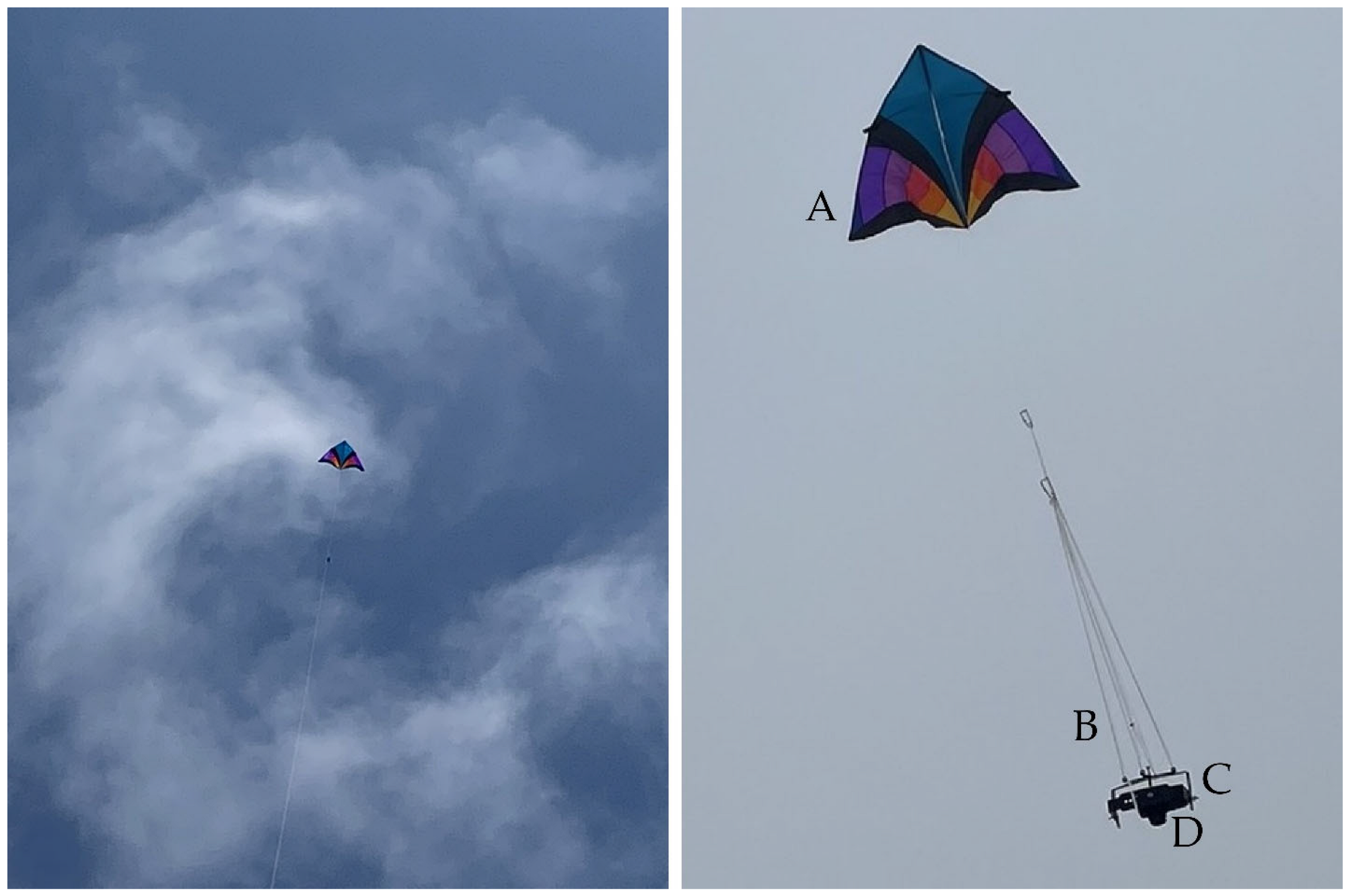
The kite aerial photography survey method we employed required a kite, kite line and spool, a camera with intervalometer capability, a rig to attach the camera to the kite line, a camera box, ground control points, and real-time kinematic (RTK) GNSS equipment. The kite used for the first three surveys was a Hi Sky Delta (Hi-Flier Manufacturing Co. (Decatur, IL, USA)) (213 × 106 cm, 7 × 3.5 ft) with 45 kg (100 lb) line; later, the kite used was a Levitation Delta (Into The Wind (Boulder, CO, USA)) of the same size (see Figure 3), with 68 kg (150 lb) line and a spool with a winder for controlling the kite. The camera used was a Canon PowerShot S95 (Canon Inc. (Ota, Tokyo, Japan)), especially suitable for SfM due to its global shutter sensor [33,67], with the Canon Hack Development Kit (CHDK) firmware update, which includes an intervalometer for photo capture at a predefined time interval [68]. A Picavet rig and camera box were used to attach the camera to the kite line and to help to stabilize the camera in high and irregular winds. The general camera settings used were low ISO, low aperture (F-Stop), fast shutter speed, and manual focus set to infinity. These settings ensure high-quality and sharp images, especially due to the fast shutter speed and manual focus. For all surveys, camera settings were adjusted manually for consistency across all images and were adapted based on field conditions to balance exposure as needed.
Based on the desired ground sampling distance (GSD) and parameters, including the field of view, camera angles, pixel size, scene width and length, and other KAP-based parameters, we aimed for a camera height between 60 and 90 m. Spatial resolutions less than 10 cm typically require altitudes lower than 100 m; other KAP-based surveys reviewed a range in flying heights between 10 and 180 m, with most between 50 and 100 m [1,3,69,70,71,72]. Flying heights were also adjusted based on field conditions. On a particularly foggy and misty day (August survey), the kite was flown lower so as not to compromise clarity in the imagery by flying at an altitude where the fog would obscure the photographs. The Picavet rig was placed on the kite line about 10 m below the kite for stabilizing the camera and ensuring a clear field of view.
Given the formula for GSD (assuming vertical camera angle at nadir), where h = height above ground level (AGL), p = pixel size on the camera sensor, and f = focal length, we can solve for average height AGL using the ground pixel size derived for the photogrammetric results as the GSD.
G S D = h × p f
h = G S D × f p
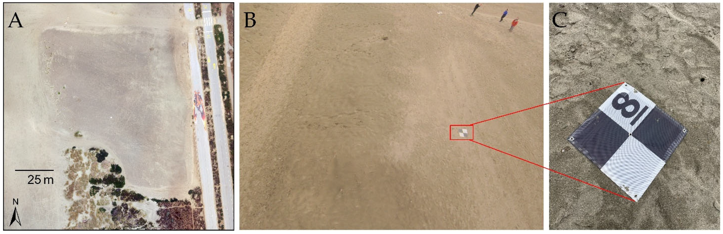
We used between 9 and 12 ground control points (GCPs) for each survey, which is consistent with or denser than the number used in similar studies [4,5]. Ground control points were established using 0.6 by 0.6 m black and white checker targets labeled with numbers for easier visual identification during processing in Pix4Dmapper (see Figure 4). GCP locations were collected in NAD83 (2011), based on the datum used by a nearby base station, accessed via NTRIP (Networked Transport of RTCM [Radio Technical Commission for Maritime Services] via Internet Protocol) [73,74]. Geolocation information was collected using an RTK-GNSS (EOS Arrow Gold) receiver set to stream NTRIP data, which delivers highly precise location information at about 1 cm 3D accuracy, in part thanks to the proximity of the base station. GCP data points (id, x, y, z, horizontal precision, vertical precision) were collected in ArcGIS Field Maps (version 25) prior to each KAP flight.

2.3. Data Processing

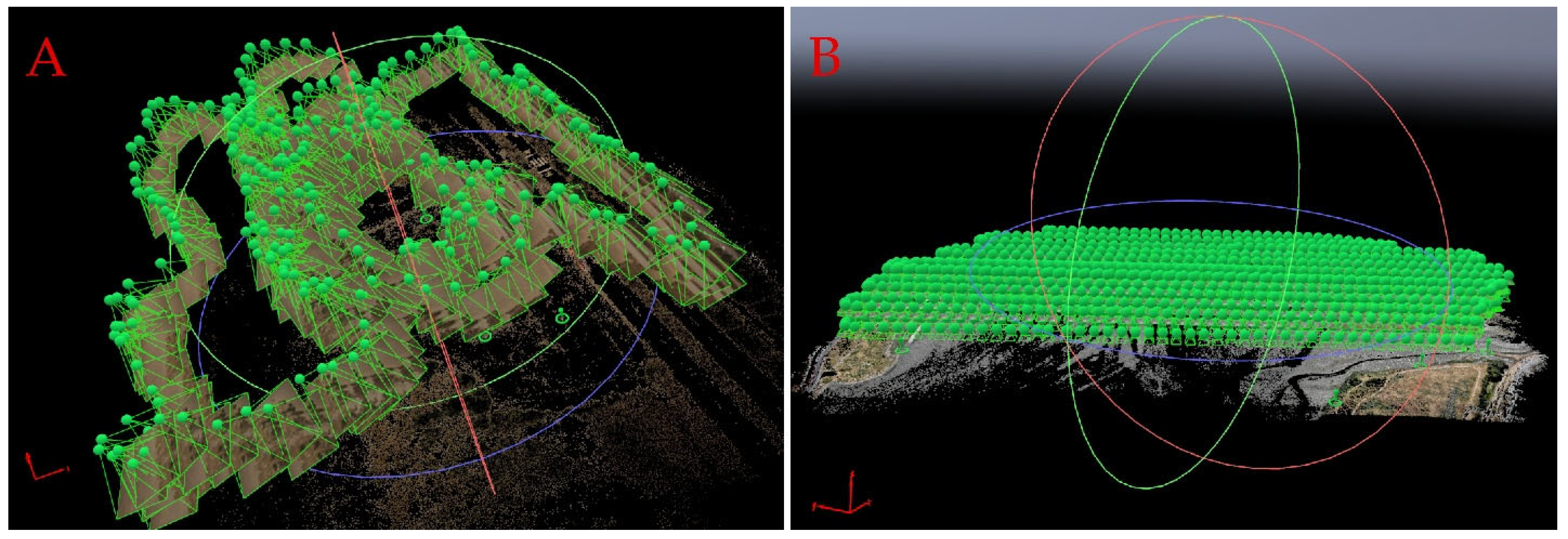
The photogrammetry software Pix4Dmapper (version 4.10.1) was used for processing the individual images and ground control points for each survey. Prior to bringing the GCPs into Pix4Dmapper, horizontal coordinates were referenced to NAD83 (2011) Universal Transverse Mercator (UTM) Zone 10, using the same datum as the base station, and the vertical datum to NAVD88 for mean sea level in meters. The GNSS receiver provides the vertical datum as Height Above Ellipsoid (HAE), which is converted to NAVD88 by subtracting the local geoid height (−32.4) determined using an online geoid height calculator from UNAVCO (https://unavco.org/software/geodetic-utilities/geoid-height-calculator/geoid-height-calculator.html (accessed on 6 Feb 2025)). Pix4Dmapper also generates a quality report as part of the processing process, which includes point cloud density and the horizontal and vertical root mean square error (RMSE) of the GCPs. Although the flight planning of image front- and side-lap at defined flying heights similar to that used with drones was not possible, the quality report for the October 2025 capture (displayed in Figure 5A) identified that 97% of images were calibrated, with a median of 212,285 key points per image, a median of 2788 matches attained per calibrated image, and a mean RMSE of 0.012 m for 12 well-distributed GCPs.
Because of the manual nature of KAP, each of the five surveys covers a slightly different area, in part due to variations in flight path (Figure 5), as opposed to drone surveys, for which one can program a flight path and height, and for which the resulting outputs have consistent extents. Table 1 shows the ground sampling distance, number of photographs, RMSE, area covered, and average camera height, which differed between surveys.
After processing in Pix4Dmapper, the data outputs are (1) digital elevation models and (2) high-resolution imagery. Here, DEMs refer to digital surface models (DSMs), as opposed to digital terrain (also called bare earth) models. DSMs can include surface features like vegetation, whereas bare earth models have those features ‘removed’. For this study, we used digital surface models; during the study period, vegetation was not yet very established and DEMs were clipped to the fenced area to focus on volumetric change where the embankment was mostly bare earth.
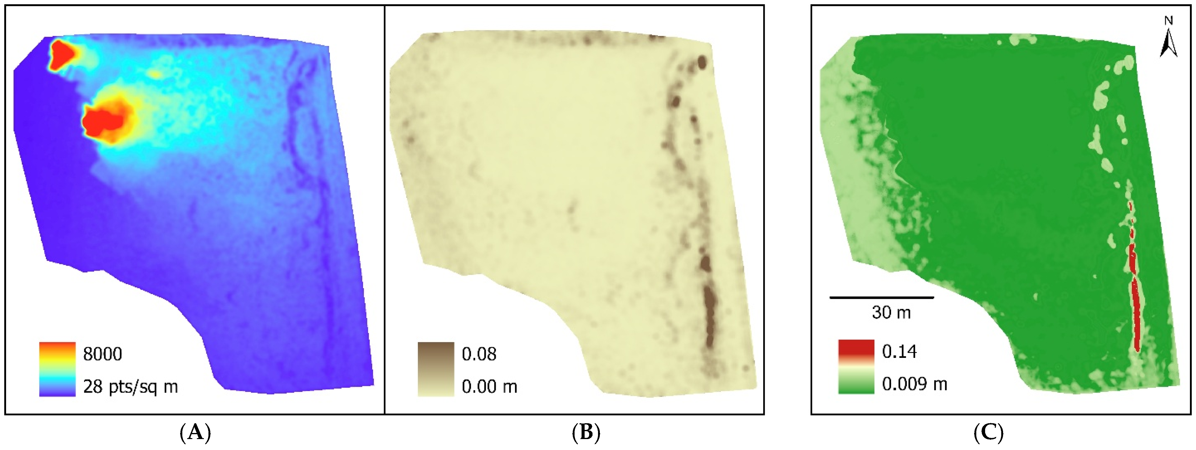
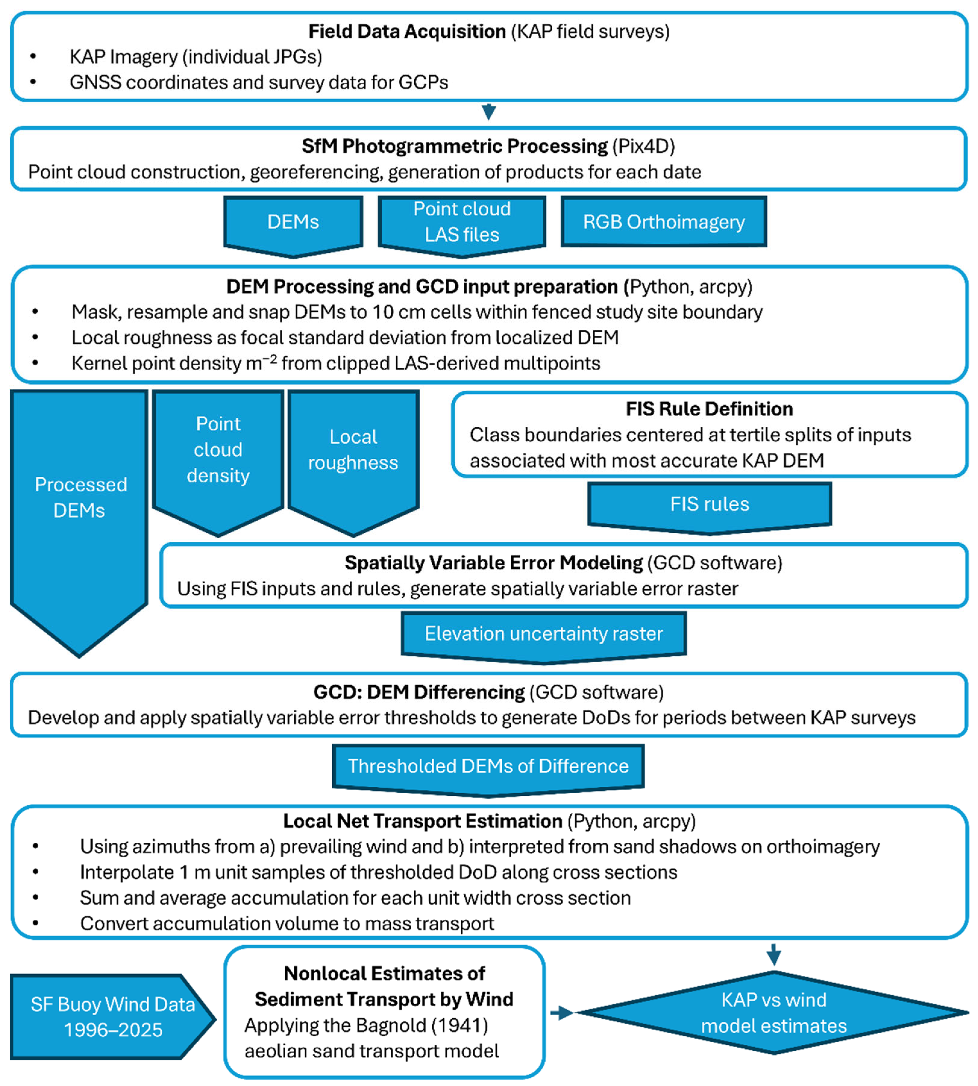
Figure 6 shows the workflow from data acquisition through analysis. Python (Jupyter) notebooks (version 3.13.7) with the arcpy module from ArcGIS Pro 3.6 (Esri Inc., Redlands, CA, USA) were developed to process the DEM outputs from Pix4Dmapper to create suitable inputs for use in geomorphic change detection. Imagery and DEMs were clipped and resampled to a consistent extent and pixel size (0.1 m). For the DEMs and all other GCD inputs, this also involved defining a polygon mask within a fence around the revegetation area and aligning the cells with a snap raster. This allows for comparison across surveys on a cell-by-cell basis because all resulting DEMs and GCD inputs have the same extent, cell size, and cell alignment. A local DEM roughness raster was developed by employing the standard deviation method [75] applied to a local DEM. We created the local DEM in a similar manner to detrending [27], but instead used a 1 m circular focal mean instead of a low-order polynomial surface to subtract from the DEM. The focal mean DEM was also used to create a more generalized slope raster. For point density, we used the LAS point cloud output from Pix4Dmapper, converting this to multipoints, then to points, and finally a kernel density, generating output points per square meter.

2.4. Data Analysis

Data analysis involved error assessment and geomorphic change detection (using Geomorphic Change Detection, GCD Standalone version 7.5, from Riverscapes Consortium, Logan, UT, USA) to derive thresholded DoDs, followed by subsequent analysis using Python notebooks in ArcGIS Pro 3.6 with the arcpy module to evaluate volumetric and mass change from sediment transport along downwind cross sections with wind azimuths set both from the 310° prevailing wind direction at the SF buoy and interpreted from sand shadows in orthoimagery developed in this study.

2.4.1. Accuracy Assessment

Error can be the result of various factors, including low point cloud density, steep slope, insufficient coverage, the density or accuracy of GCPs, or KAP flight behavior. We conducted accuracy assessments to measure error in the DEMs by comparing independently collected ground survey data with KAP-derived elevation values. Two assessments were conducted: a leveling survey as part of the 16 June data collection, and a scattered points survey during the 30 October data collection. The two separate methods for assessment also serve to further test the consistency and uncertainty of the KAP-derived data.
The leveling survey consisted of four transects from the center GCP to each of the four corner GCPs (northwest, northeast, southwest, southeast). A tape was stretched from the center out to each of the four corners, and data points were recorded along the four lines, spaced a few meters apart. Measurements were taken using a Topcon DL-503 digital level (vertical error 1.5 mm standard deviation over a 1 km double run with the BGS50 leveling rod used). The October accuracy assessment was conducted by surveying 39 scattered point locations using the GNSS receiver, the same device used for GCP data collection. These points were not used in processing the model.
These accuracy assessments can be used to inform limitations to the use of the methods, as they are assumed to be random errors. Systematic errors were also assessed where possible, such as a +0.36 m bias in the August DEM detected in an area of elevation stability resulting from erosion to the resistant embankment, affecting both August–June and October–August DoDs; this offset was subtracted and new DoDs created for further analysis.
In addition, Pix4Dmapper generates RMSE as part of model processing (see Table 1). This is the measure of error comparing the ground control points in the model to their true position. As an additional accuracy check, we reprocessed the model for each survey after reassigning a subsection of the GCPs as independent checkpoints to assess their vertical accuracy without contributing to the model creation (see Figure 4). We chose targets which covered lower elevations and where there would still be a reasonable distribution of GCPs over the embankment area. The final model used for analysis included all GCPs.
The independent accuracy assessments and RMSE of the GCPs and checkpoints were used to inform a minLoD uncertainty threshold for geomorphic change detection.

2.4.2. Spatially Variable Error

In addition to applying minLoD thresholds, we conducted spatially variable error modeling using a fuzzy inference system in the Geomorphic Change Detection software. Raster inputs commonly used for FIS thresholding in geomorphic change detection are point density, slope, and roughness [38,75]. In the original FIS rules, Wheaton et al. [38] use point density to refer to survey points from total stations or scattered GNSS points, while more recently LiDAR or SfM point clouds have been employed, with densities higher by orders of magnitude than survey points; our densities were commonly over a thousand per square meter at the 95th percentile. Relatively flat landforms are commonly areas of reliable elevation detection, so slope angle, easily derived from a DEM, is commonly used in a geomorphic change detection analysis employing FIS [75]. The availability of terrestrial laser scanning and airborne LiDAR has provided roughness estimates that can be used to identify deposits like coarse river gravels [75], breaks in slope and other geomorphic elements that can contribute effectively in a fuzzy inference classification [75].
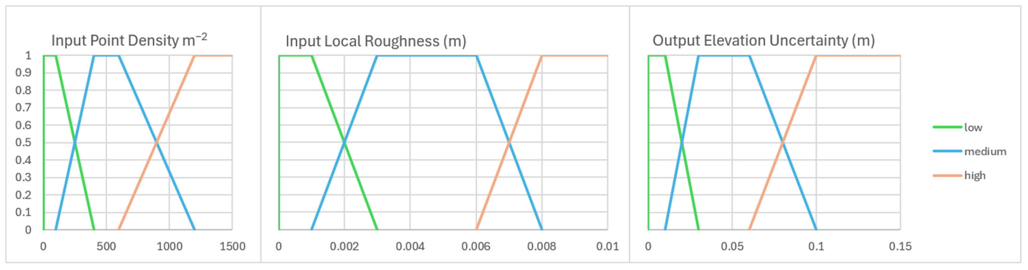
In our study site, roughness may be telling us more than slope as a source of error. With dry sands, dune slip faces typically reach an angle of repose of approximately 35° [76] and, along the eastern edge of our dunes, the slopes are often even steeper, especially if moisture is a factor, which it often is in foggy San Francisco. However, our study site is too small to consider variations in wetness as an additional FIS input, and, if slope as a factor relates mostly to local anomalies of high slope resulting from errors, then excluding high slopes would exclude real parts of the landscape. After experimentation, we used a model employing point density and roughness alone (see Figure 7), applying the local DEM roughness measure described above. Figure 8 shows the FIS categories and Table 2 shows the rules used to build the model.

2.4.3. Geomorphic Change Detection

After error modeling, we assessed geomorphic change using DEM Differencing, a technique used for evaluating changes in deposition and erosion on a surface between repeat topographic surveys [77]. DEM Differencing can show changes on a cell-by-cell basis by subtracting an earlier from a later DEM [38,77,78]. Here, it is used as a tool for understanding patterns of change in sand movement, above a given threshold.
DoDs were derived for March to October and between each survey using the GCD software to assess volumetric change over time. For March to October, we derived DoDs using several different error analyses to assess the impact on results: unthresholded (raw), uniform 10 cm and 20 cm minLoD, and spatially variable probabilistic with 80% and 95% confidence intervals based on the FIS rules. In addition to the thresholded DoD spatial results, GCD analysis results provide information on areal and volumetric change overall. For comparison between each survey, we assessed unthresholded (raw) DoDs and thresholded DoDs using the FIS model with a 95% confidence interval.

2.5. Sediment Transport by Wind

Since the relative changes in sand accumulation and erosion could be determined across the study over four periods throughout the year, approximations of sand transport rates were made using a simple form of the Bagnold equation [40],
q = C ρ g u 3 1 u * t 2 u * 2
where q is sand transport rate (kg m−1 s−1); C is the Bagnold constant, which ranges from 1.5 to 3.5, depending upon the surface sediments; ρ is atmospheric density; g is acceleration due to gravity; u*t is a threshold friction velocity to initiate sand transport (0.25 m s−1); and u* is friction velocity, which we determined from wind speed using
u = κ U ( z ) l n ( z z 0 )
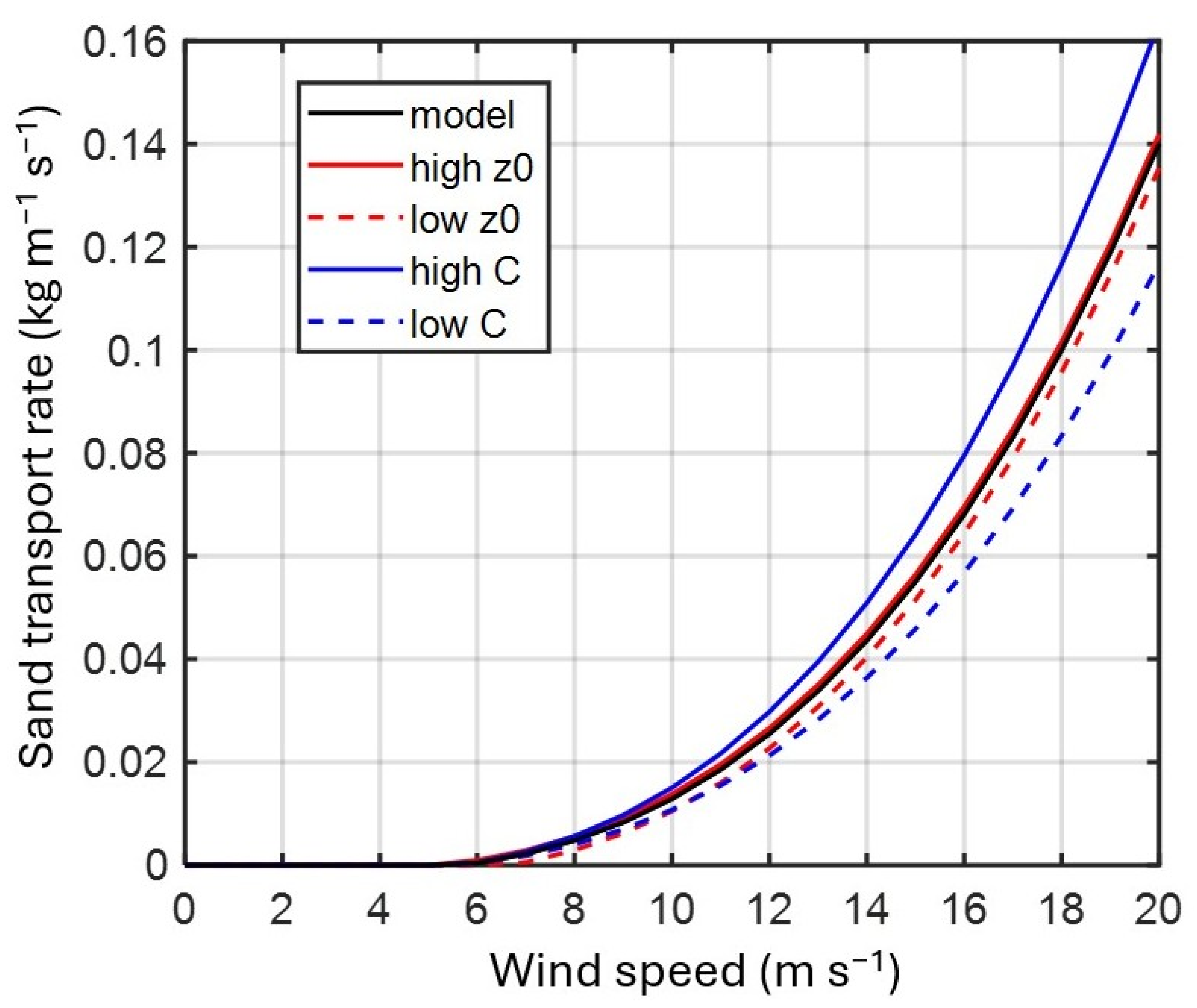
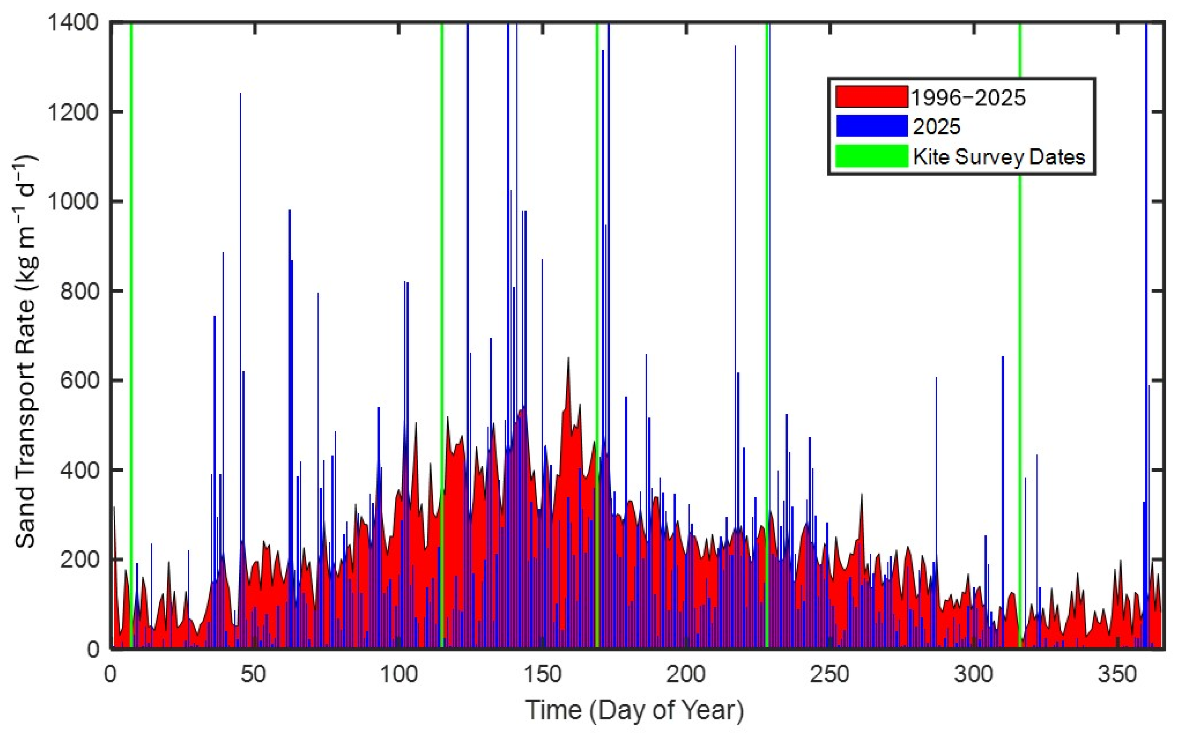
where κ is von Kármán’s constant (0.4), U is wind speed (m s−1), z is observation height, and z0 is the surface roughness length (m) [40]. Wind speed was obtained from the San Francisco Buoy (United States National Data Buoy Center (NDBC) Station 46026), located 33 km offshore from Ocean Beach. Due to some missing data in 2025, wind speeds were gap-filled using wind speed recorded at San Francisco Airport, adjusted based on linear regression between values collected simultaneously at both locations. We used C = 1.8, recommended for naturally graded dune sands with similar sand grain size [49], and approximated z0 at 0.0005 m, based on literature estimates of sand grain size of 0.2–0.3 mm for Ocean Beach [79]. Figure 9 shows the sediment transport rates estimated for Ocean Beach. Upper and lower estimates of two of the most uncertain inputs are added to illustrate the impact of some key model uncertainties on sand transport estimates for the site.

3. Results

Results include the primary outputs: high-resolution imagery and digital elevation models, results of the independent accuracy assessments, geomorphic change based on the spatially variable uncertainty thresholds, and the wind-driven transport rates as compared with the accumulation rates from the KAP-SfM survey data.
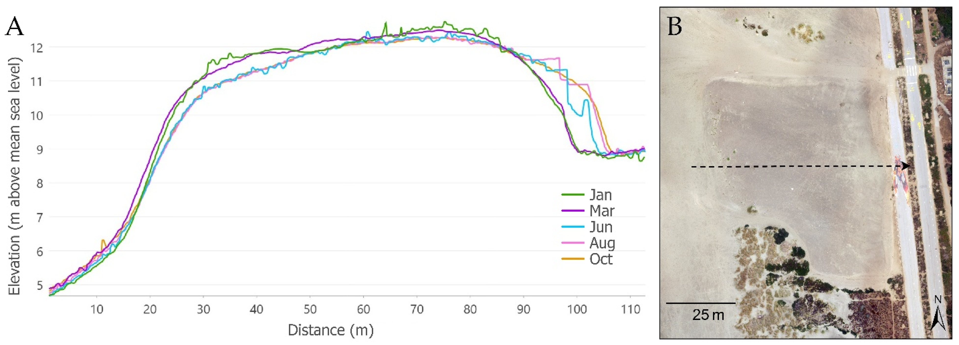
Figure 10 shows a cross-sectional profile of the embankment from west to east to compare elevations between the five KAP surveys using the unthresholded (raw) DEMs. Elevation appears relatively stable, suggesting erosion and deposition are in balance, on the lower foredune slopes (~20 m on the x-axis) and near the leeward edge of the ridge (~60 to ~80 m), but decreased at the foredune ridge windward (beach) side (~25 to ~50 m) and increased on the leeward side of the embankment (~90 to ~105 m). The greatest variance between surveys is between the 90 and 110 m positions on the x-axis, on the lee (east) side of the embankment, where there was significant deposition. Figure 10 shows little change between January and March, which may be due to stronger spring and summer winds.
In part due to the challenge of maintaining a consistent flight plan, we can expect to find areas of insufficient coverage, leading to errors. Even after smoothing with a low-pass filter and resampling the DEMs, there are visible errors in the elevation models (Figure 10). Because there has been no error analysis or threshold, spikes and dips may be from DEM noise rather than true elevation values. These surface errors are the clearest in the January elevation model, which is consistent with Pix4Dmapper-reported RMSE.

3.1. Independent Accuracy Assessments

Table 3 shows the results of the accuracy assessments comparing vertical values from ground surveys with KAP-derived elevation model values. The average random error was 4.5 cm in June and 2.9 cm in October. Error was computed at each point by subtracting the KAP-derived DEM value from the observed elevation. Systematic error was computed by averaging all error values and was −1.8 for June and −0.6 for October. Systematic error was then subtracted from all raw error readings to find random error for each point. For both assessments, the mean of all the random error values was zero, meaning the errors are equally weighted between positive and negative values, and the random error values are normally distributed.
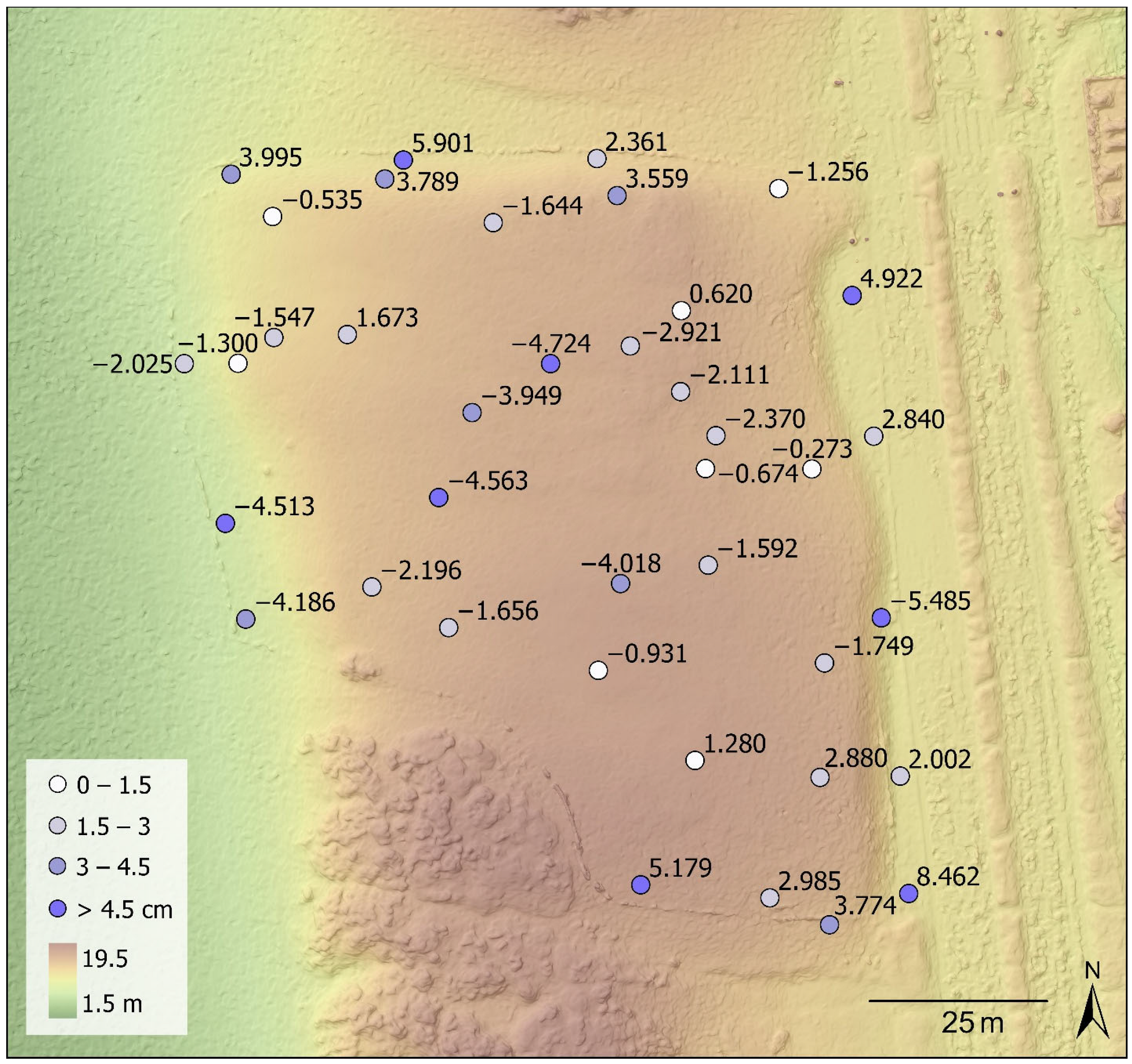
The June accuracy assessment results show random error values between −13.6 and +12.3 cm, with a mean absolute value of error of 4.5 cm and standard deviation of 3.4 cm (for absolute value of random error). The average absolute value of random error from the October accuracy assessment is lower than June at about 2.9 cm, with a range between −5.5 and 8.5 and standard deviation of 1.8 cm for absolute value of random error. Building on the accuracy assessments, the mean absolute random error (μ < 5) and overall range of values (±13) (Table 3) informed our selection of 10 and 20 cm minLoD thresholds to compare uncertainty modeling at various thresholds.
The accuracy assessments were conducted using different survey equipment and methodological design, so they are not directly comparable but rather are for comparing KAP-derived elevation to true elevation values. For this purpose, October is a more useful assessment because of the accuracy of the surveying equipment and ability to conduct spatial statistics to understand the spatial variability of error. The points also cover a wider range of elevation values, where the points along the transects mostly cover the top of the embankment where elevation values are relatively consistent.
Figure 11 shows the distribution of scattered points across the embankment, and the absolute value of random error in centimeters, and seems to show a clustering of the magnitude of error (absolute value) in particular areas. A test of spatial autocorrelation using Global Moran’s I for random error had a positive Global Moran’s I of 0.3 and p < 0.001, indicating spatial autocorrelation, which is to be expected with regional systematic bias (however small) due to local conditions of slope and landscape elements, as well as with ‘doming’ errors commonly observed in drone-based surveys [80] and especially with KAP-SfM [5]. The same test for the absolute value of random error was not found to be statistically significant, suggesting that it is more likely truly random than systematic. Still, given the irregularity between surveys, inconsistency of independent accuracy assessments, and a relatively small sample set for assessing error, we can assume there is a benefit in investigating spatial variability of error in the KAP-derived elevation models.
These validation assessments were completely independent of DEM generation, so are a more reliable test for validation than the RMSE readings reported by Pix4Dmapper. Still, the RMSE values were between 1.4 and 3.1 cm for the vertical accuracy of GCPs, and between 1.6 and 4.3 cm for checkpoints (reclassified) (Table 1). While the results of the accuracy assessment are higher than the RMSE, the results are consistent in that the October model has lower error than the June model.

3.2. Geomorphic Change

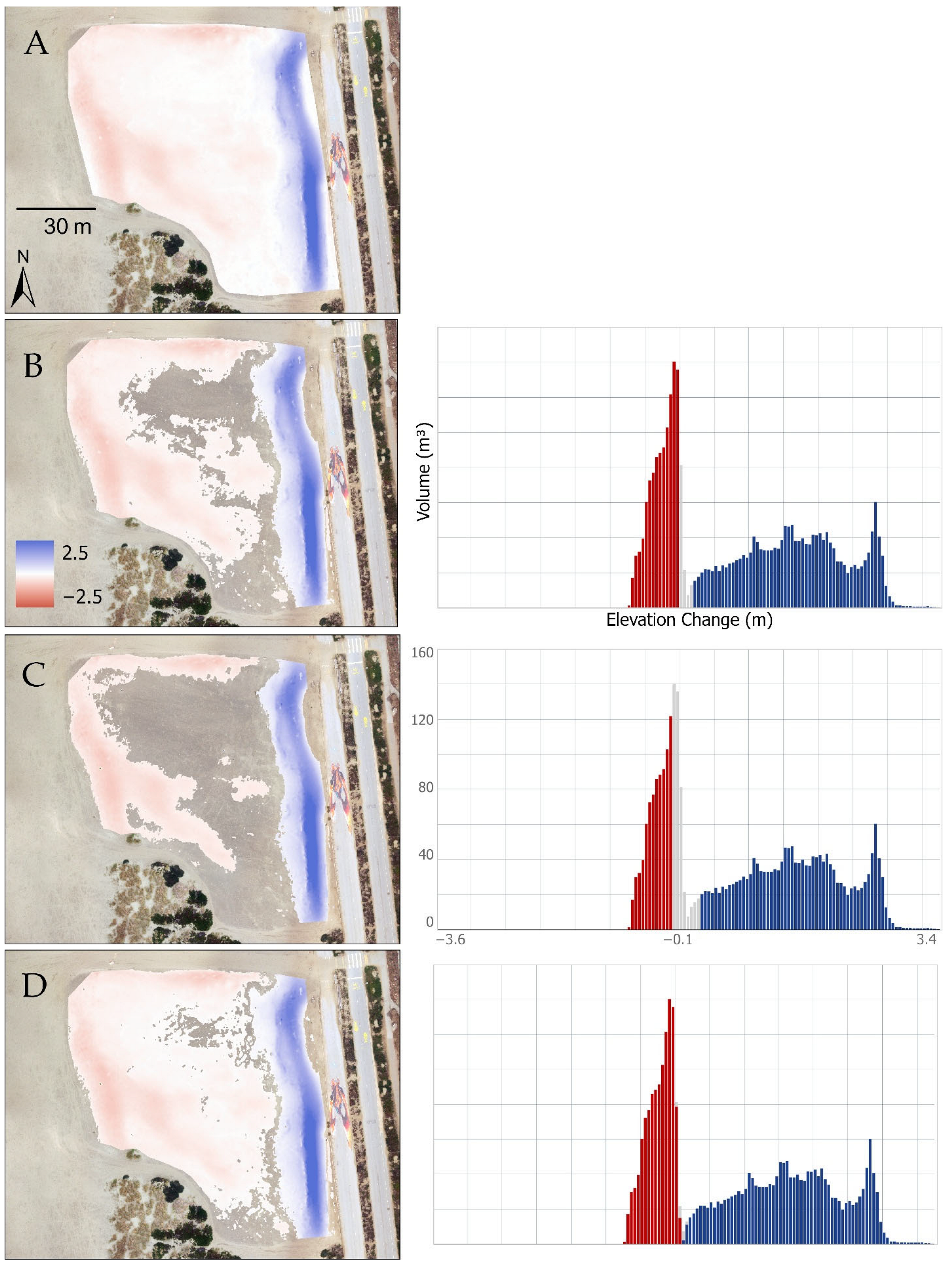
Using the DoD for March to October, we compared the results with different types of error modeling for thresholding. Table 4 shows the difference in erosion, deposition and net change for raw (no error analysis), uniform minLoD at 10 cm and 20 cm, and spatially variable probabilistic error for 80% and 95% confidence intervals based on fuzzy logic, as described in Section 2.4.2.
Figure 12 depicts the difference between these error models for the March to October DoD. It does not include the SVE visualizations for 80% CI probabilistic threshold, which was quite similar to the 95% CI (see Table 4). The minLoD uniform thresholds are the most restrictive for filtering the DoD surface. The March and October surveys had the least visible surface error, based on the visual representations of the model, and had the lowest RMSE (1.4 and 2.2, respectively) (see Table 1). The DoD shows sand movement east and some moderate erosion over the surface and along the western, southern, and northern edges of the study area. These results, seen also in Figure 10, exhibit distinct north–south banding, with the greatest geomorphic change being net deposition on the leeward edge. There is moderate erosion on the western side of the dune toe and on the top surface of the embankment where wind is accelerating due to terrain conditions, and deposition occurring on the leeward side of the foredune where wind is decreasing. Here, even raw DoD results showed the magnitude of sand movement landward is in meters, where mean error is below 5 cm.
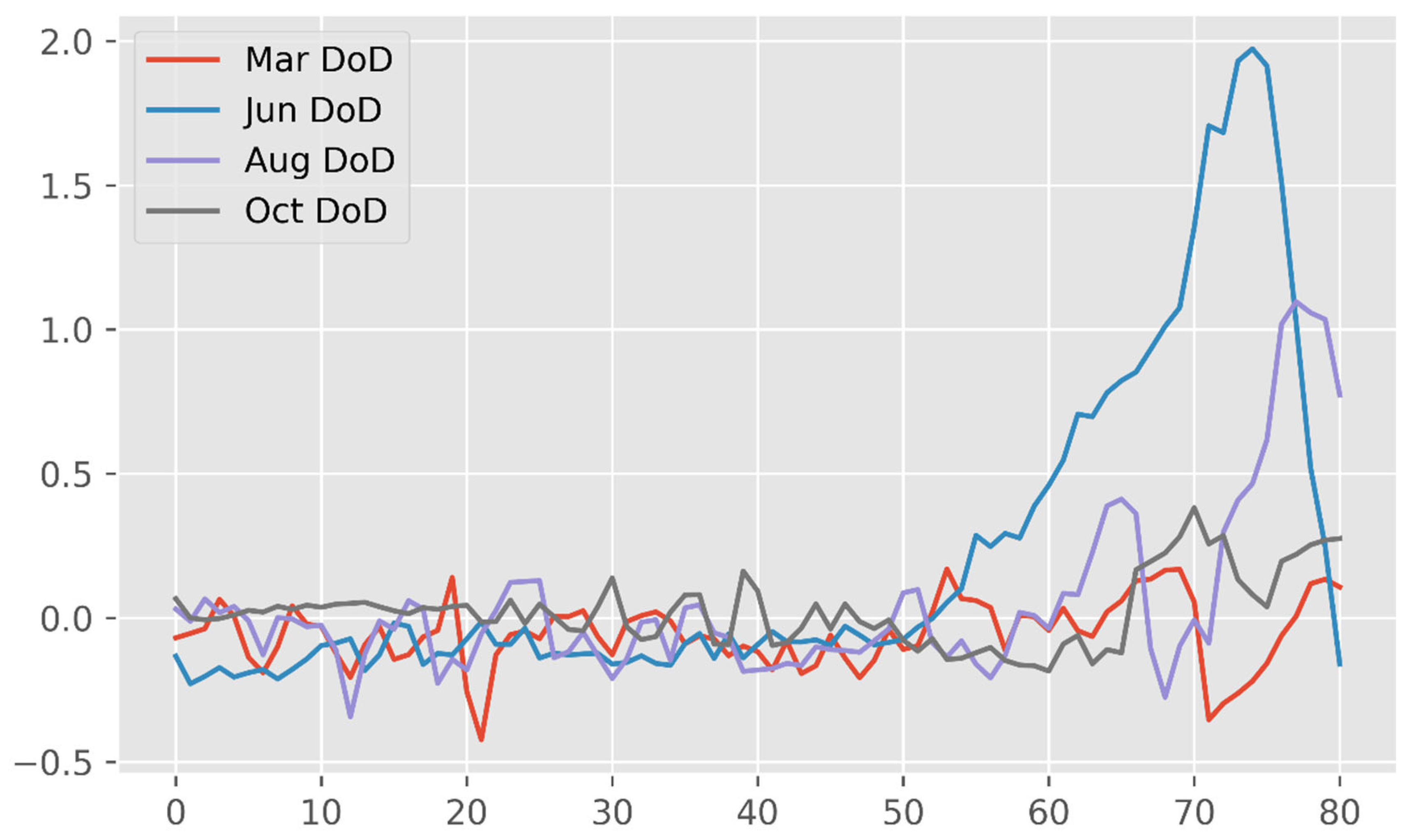
Based on the results shown in Table 4 and the similarity of the probabilistic thresholds with 80% CI and 95%, we used the FIS rules-based error threshold for the other DoDs. Table 5 shows geomorphic change results between each survey from the raw DoD and thresholded DoD (95% CI). The greatest volumetric change in deposition occurred between March and June on the landward edge of embankment, though that is not the highest net change period because a similar level of erosion also occurred.
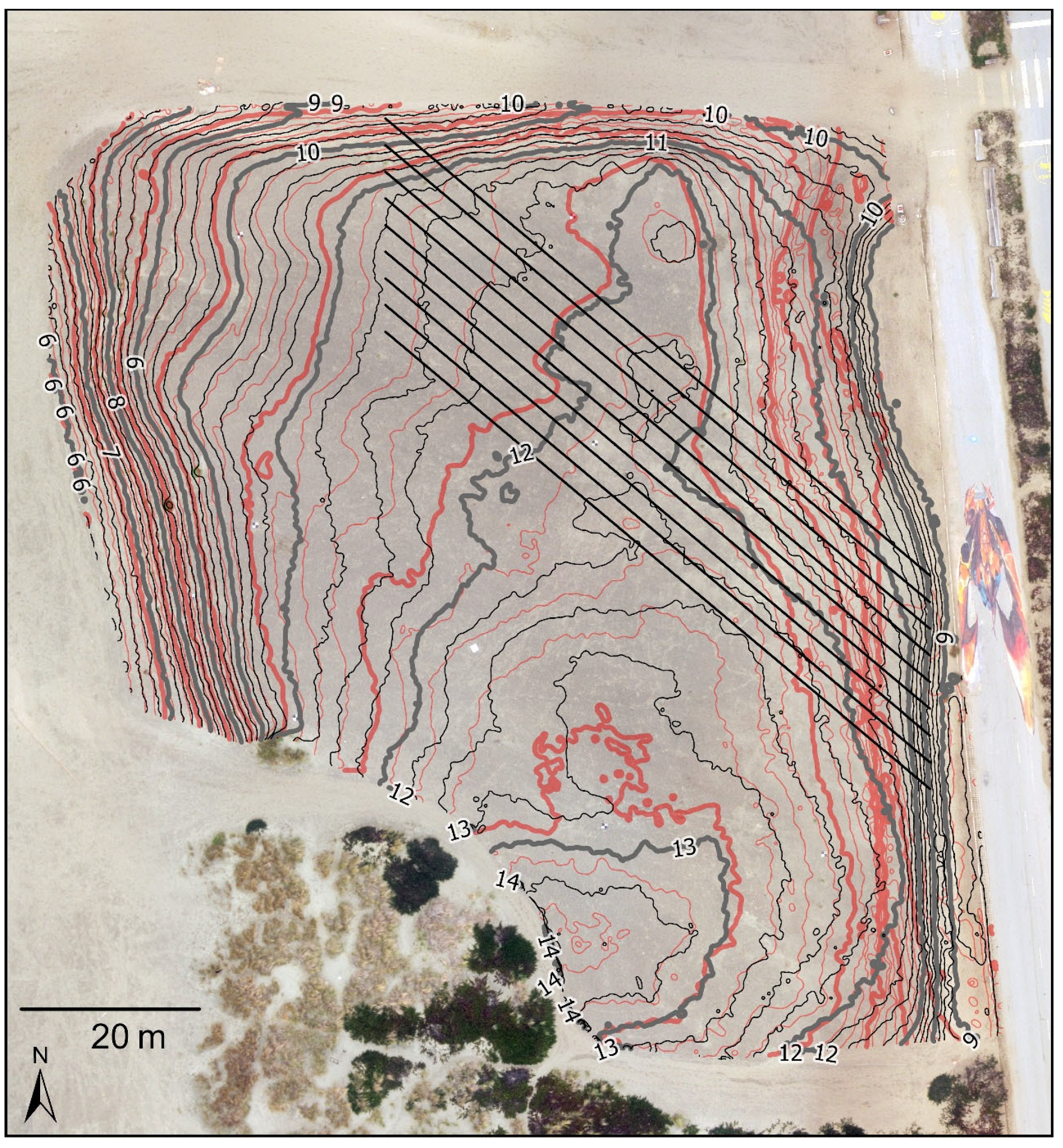
To assess the overall downwind sediment transport and illustrate areas of net erosion and deposition, we created nine upwind to downwind cross-sections spaced 3 m apart, all covering the greatest extent (80 m) of the embankment feature in the downwind direction, where the downwind azimuth is based on the prevailing wind direction at the SF Buoy, 310° (Figure 13). This allows us to compare the four sampling periods and visualize the landward system of sand migration in a seasonal context (Figure 14). The largest accumulation is seen in the Mar–Jun period, but this was also the longest number of days (95), as opposed to 65 (March–January), 61 (August–June), and 75 (October–August). We also derived cross sections based on wind directions based on sand shadow evidence on our orthoimagery collected in March (290°), June (270°), August (260°) and October (280°), and used these for alternative estimates of sand migration for the respective time periods ending in those months.

3.3. Wind-Driven Transport Rate Estimates for Ocean Beach

An estimation was made for daily average sediment transport rates using the Bagnold equation (Equation (3)) [40] based on wind data from the San Francisco Buoy for both the year of study (2025) and the 30 yr record from 1996 to 2025 (see Figure 15; Section 2.5 for details). These magnitudes are generally comparable to those found for aeolian sand transport rates published elsewhere [81,82,83]. The estimate for the annual total sediment transport by wind on Ocean Beach in 2025 was 77 Mg m−1 a−1, which was slightly lower than the long-term average of 79.5 Mg m−1 a−1. In both the long-term record and in 2025, sediment transport was highest during spring, followed by the summer. The number of hours of wind speed above the entrainment threshold at Ocean Beach declined steadily as wind speed increased, yet the transport rate increased exponentially (Figure 9). The resulting sediment transport frequency across wind speeds was normally distributed and peaked at 10 m s−1. Winds in the range of 8–12 m s−1 alone were responsible for 72% of the sediment transport over the year despite occurring for only 18% of hours. June had the greatest number of hours with wind speeds in the range 8–12 m s−1, followed by May, July, August, and April, and this trend was the same for the 3-year record.
The mean rate of sediment transport for the four periods that lie between kite survey dates is provided in Table 6. Spring (Mar to Jun) was the period with strongest average wind-driven transport, closely followed by summer (15% lower), with winter and autumn months producing significantly lower rates (52% and 58% respectively).

Accumulation-Derived Transport Rates from Kite Survey DoDs

In this study, positive DoD values (accumulation cells) can be seen to be most likely to produce the clearest indication of sand transport, both in the raw DoD and in the thresholded DoDs, where the lower magnitude erosional cells are more commonly excluded by the threshold (Figure 12). This is to be expected from an understanding of dune development processes [40] and consideration that our study site is not a closed system. Thus, our spatial analysis of downwind sediment transport using cross-section data focused only on accumulation cells, where DoD > 0.
Using a density of quartz 2650 kg m−3 and a beach dune porosity of 0.356 from Lopez et al. [84], we derived mass in kg for a unit square meter as
m a s s = D o D 1 0.356 2650
While the accumulation of sand detected in cross-sections of the DoDs is not the same as transport rate, since accumulation results from the balance of deposition and erosion, it does tell us about net transport detected on that part of the dune, typically more on the southeastern edge of the cross-sections (Figure 13); accumulation represents what passes through a width of 1 m in that zone. Table 6 displays sediment mass accumulation rates in two ways, based upon different assumptions about the meaning of the analysis: (a) individual cell results assume that we are looking only at an individual square meter, while (b) looks at sand transport through the cross-section, considered as transport either the entry or exit cell, with a unit 1 m width. Essentially, the accumulation cells downwind serve as a capture system for sediment that passes through the unit-width cross-section entry, but neither method captures all the transport. The former ends up with a very low rate compared to the wind model due to the open system and inability to quantify what goes through, while the latter accumulation can end up deposited anywhere along the cross-section, which lessens the effect of the open system.
Accumulation capture for either assumption is consistently less than the modeled prediction of total sand transport rates, but the through-section assumption predicted between 64% and 80% of the wind model prediction. This is to be expected with sand lost from the open system. In fact, sand is removed annually from the roadway immediately to the east of the study site to maintain accessway [85]. As with the wind-driven estimates of sand transport rates in the previous section, the largest net accumulation rates occurred during spring, followed by summer, with an order of magnitude drop to winter and autumn months. Nevertheless, with only four periods to compare, the wind-driven sand transport estimates scale closely with the observed accumulation rates (Table 6) over time, with very high R2 values for either assumption.

4. Discussion

This study focuses on two separate goals to which KAP surveys are applied: (1) assessing the accuracy of the method for geomorphic change detection for monitoring the revegetation project, and (2) understanding the sand transport system of the dunes, including estimating sediment transport to compare with wind modeled rates. While there is always a measure of uncertainty, the exploration of error in these data showed relatively small uncertainty relative to the differences observed, suggesting that DoDs from KAP surveys can provide meaningful information on erosion and deposition trends and sediment volumetric change.

4.1. Sand Migration and Geomorphic Change

The dune system experienced a high magnitude of sand migration. Our results show several meters of sand movement landward, even after various types of error modeling and with the most restrictive uniform 20 cm minLoD threshold. The results of the independent accuracy assessment also have a mean error (μ < 5 cm) well below the magnitude of geomorphic change observed.
Dune migration landward is expected and consistent with the scientific and management-related literature on Ocean Beach [52,59,62], and our study allows us to visualize this phenomenon spatially and to understand seasonal accumulation rates. That the wind model estimates of sand transport scaled closely with accumulation rates over the year provides an independent cross-check to the KAP-derived estimates of sediment accumulation changes over time and may allow us to assess past blowout events from archived buoy data. There is clearly a net loss of sand landward of the study site given the observed accumulation of sand accounted for only about 48% of the total estimated sediment transport. This is further corroborated by the observation of sand excavation from the roadway immediately east of the study area following strong wind events.
In terms of implications for the revegetation project and for dune grass survival, we know that sand accretion should be at a level where there is some burial, which supports plant growth, but not so much accretion that sand will bury and subsequently kill plants [86]. Most of the transplants on the eastern slope of the sand embankment where deposition occurred were fully buried and did not survive. Though not reported here, parallel studies that consider biotic factors are investigating plant survival, employing both the KAP imagery and field observations [61], with sand shadows clearly visible in the high-resolution imagery. Observed plant survivorship is clustered along the western and northern edges of the embankment where there has also been lateral clonal expansion, consistent with the literature on the expected growth area for native embryonic foredunes on the seaward slope [46,86,87]. The GCD results also show the greatest stability in some of the most vegetated areas, likely due to the stabilizing influence of both the marram grass with deep roots as well as the long, laterally expanding rhizomes of Leymus mollis.
At this stage, it cannot be said what effect the revegetation or individual transplants are having at the scale of volumetric change, and indeed longer-term and continued aerial and field surveying will be necessary for assessment at that scale. It would be interesting to see whether sand is migrating at similar rates landward at other similarly sized dune areas at Ocean Beach, in particular where there are hotspots for sand encroachment onto the promenade. One would expect that most of the dune encroachment onto the road is occurring in the largest blowouts and where the sand embankments are less densely vegetated. Additional research could compare wind-based models with observed sediment transport on different dune types at different levels of vegetation cover. As vegetation becomes more established, future studies at this site could compare rates of transport to assess whether vegetation leads to meaningful change in sediment transport and at what point it becomes significant.
In understanding sand transport in this evolving dune system, the second goal of our study, the site experiences more sand movement landward during seasons with heavier onshore wind (from the northwest) during spring and summer. However, the study site is part of a larger system where sand movement is more complex than the localized southeastward movement occurring at the site. At Ocean Beach, the general trend is wave-driven beach erosion in winter and accretion in the summer and fall, and progradation in the northern half and retrogradation in the south [52,62]. Further, patterns of sand movement change from year to year, depending on factors like ENSO, which affect winter storm wave environments, seasonal wind speeds and direction, winter precipitation and sediment supply. As we have documented, while DoDs provide a picture of the effect of wind transport, the open system makes it an imperfect measurement of the transport rate, representing approximately half of what is predicted from wind models. However, seasonal and spatial patterns are clearly illustrated. The comparison of wind-driven sand transport between 2025 and the 30 yr record suggests the year of this study was close to, but slightly lower than, the average for sand transport based on observed wind speeds. Though 2025 was seasonally consistent with the long-term record, the comparison also shows that sand transport is dominated by distinct wind events, with strong day-to-day variability.

4.2. Assessment of Kite-Based Method

While we did not conduct congruent drone-based UAV surveys, our study is consistent with centimeter-scale accuracy previously demonstrated in successful KAP-SfM applications using similar survey-grade geolocation equipment. While studies that conducted direct comparisons found that drone-derived data generally had lower error and uncertainty [3,4,5], KAP data still produced viable results, with vertical RMSE under 6 cm [3,4] and uncertainty budgets between 2 and 7 cm [5]. KAP presents challenges related to consistency and general predictability, relying on appropriate wind and meteorological conditions. Unlike a drone, it is not possible to automate a flight path for KAP: a break or change in the wind, a pedestrian, or a dip in the dune all have an impact on flight path and stability. Micrometeorological conditions such as turbulence also impact kite-flying capability, especially near buildings. Given the limitation of suitable sample dates to times with sufficient and consistent wind for KAP, it was impossible to create equal sampling periods. Another particularity of KAP is the need to use a lightweight camera, which in our case required a camera firmware update that provided an intervalometer.
Some limitations and particularities of our study included the relatively small number of validation points in early KAP flights, as our study methods were being developed at the same time as the restoration project was underway, also coincident with a marked increase in recreational use due to the conversion of a highway to a city park. While the eastern margin was still a highway during early flights, we needed to limit kite operation walks to the beach side, though this turned into a benefit of biasing sample dates to times of more stable onshore winds, which fortunately occurred frequently enough to capture the four periods in our sampling design.
While there are many limitations, there are also clear advantages to KAP, including the potential for a semi-random variability of camera angles and flight path that could be beneficial for SfM photogrammetry, but especially the ability to conduct surveys in areas where drones cannot fly, the low energy usage and cost, the relative ease of material procurement, and the application potential in ecologically sensitive areas.
Regardless of whether a kite or drone is used, error and uncertainty continue to vary, depending on factors including equipment, survey design, ground control placement, processing, and terrain. There are several ways to improve accuracy in KAP-based studies. Error is related to the placement and density of ground control points, as well as the positioning equipment used. Our study benefited from the use of a high-precision RTK-GNSS receiver, used in NTRIP mode, with a nearby base station providing ~1 cm vertical accuracy, coupled with carefully planned GCP placement. Other ways to reduce error include lower flights (though this can dramatically increase flight times and create greater demands on camera battery), using different kites for varying wind speeds and conditions, and taking more photographs during each flight. Though not as well-documented, lower camera placement (15–30 m below kite) may reduce error by minimizing the impact of vibrations and sudden movements for a more stable flight [88].
Consistent and moderate wind speeds are required for successful repeat topographic surveys using KAP. Winds along coastlines commonly meet this requirement, with low frictional drag over the water surface and the development of a diurnal sea breeze circulation across the coastline. These circulations produce moderate onshore flows during the day, which tend to build in speed from midmorning until late afternoon, a pattern that is repeated in coastal locations throughout the world [89]. The wind patterns in our study site, as depicted in Figure 1D, provided ideal KAP flying conditions, with very consistent W-to-NW moderate-strength winds. The range of wind speeds during daylight hours allows users to find appropriate wind speeds for a wide range of kite designs. Kite sondes have been successfully used in meteorological studies focusing on sea breezes elsewhere, though mostly during daylight hours because the nocturnal land breeze is typically too weak for successful kite flying [90]. Furthermore, the consistent onshore direction allows the KAP researcher to use the accessible beach area to fly the kite while ensuring the images capture the foredune study site well.
We found the ideal wind is onshore wind, blowing from the west at about 21 to 29 km per hour (13–18 mi/h). In winds below 20 km per hour (12.5 mi/h), the kite flies well but loses its stability and ability to lift the Picavet rig and camera; above 29 to 32 km per hour (18–20 mi/h), patterns become erratic and too powerful for the kite line and for a steady flight.
One effect of the irregular flight path and difficulty in assessing the kite position is a highly variable point density, with a possibility of major gaps in coverage. During our fieldwork, we developed improvements in methods, one of which was the use of a visual observer connected by radio to the kite flyer to aid in monitoring kite height with a laser rangefinder and communicating guidance information to help to position the kite and camera over the planned flight path. While we explored this general method during all our flights, finding the best vantage point path and field protocol was developed over time; our best results were derived from the final survey, in October. Unfortunately, the August flight had significant gaps over the main accumulation areas, and we could not know this until we had processed the imagery. Given the many challenges in finding the right winds at the right time of day (with available personnel), an important capture may be missed. Fortunately, the FIS probabilistic thresholding model still produced useful DoDs for the two periods affected (October–August, August–June), with a higher correlation with the wind model than seen with the unthresholded DoD.

4.2.1. Application of Spatially Variable Error Modeling

The most important thing in KAP-SfM workflows is understanding the potential sources of error and their spatial distribution where predictable by topographic conditions and data quality measures (such as point cloud density). Prior KAP studies have typically dealt with uncertainty by quantifying error through comparison with independent checkpoints and other data sources. We examined three different accuracy measures: vertical RMSE, independent validation points, and error modeling. While error modeling and uncertainty thresholds have become integrated into UAS-SfM workflows, they are largely absent from KAP-based surveying, save for a handful of studies. Duffy et al. [4] used precision mapping [30] for a spatially variable uncertainty threshold, and Hilgendorf et al. [5] used a uniform uncertainty budget based on GCP error, RTK accuracy, and RMSE. We build on this work by adapting Wheaton’s FIS spatially variable error model for KAP [40]. When using DSMs, vegetation and other surface characteristics can impact DEM quality, so we aimed in part to reduce the impact of vegetation by using roughness as a parameter in error modeling [26], without explicitly including vegetation. Local roughness may also be a better predictor of general collection error than slope on dunes with many smooth yet steep surfaces. Others have built on Wheaton’s original model (applied to more sparse point capture) and created more sophisticated FIS rules with additional inputs, including vegetation and wetness [91,92]. The FIS system could be further developed for application in KAP-SfM in more complex hydrological, ecological, and geomorphological environments. After exploring alternatives, however, our final FIS rules were purposefully minimal, relying only on point cloud density and surface roughness, given that error tends to be higher in areas of high roughness and sparse survey point density [38,77,93]; a small number of dimensions allows rules to be defined clearly.

4.2.2. Practical Implications

The question of scale is critical in the determination of methods for environmental monitoring. For geomorphic change studies, the magnitude of change determines the level of reasonable error, scale, and precision required of the methods. As described, there have been great advancements in the use of satellite imagery for habitat- and landscape-level modeling and the integration of large processing models for feature identification and classification [94,95]. Still, at the plot scale and particularly for GCD, there is no replacement for localized studies, which require detailed and precise monitoring.
Our study demonstrates the viability of KAP-based surveying for high-precision coastal dune monitoring, combining KAP-SfM workflows with spatially variable error modeling using fuzzy logic for GCD, greatly improving the reliability and accuracy of results for understanding sediment transport and geomorphic change at this scale. KAP methods, similar to other remote sensing methods, can be further strengthened when combined with field survey observations or applied to broader landscape scales when combined with satellite imagery [7].
Future work could follow a similar model for study sites that are sensitive to drone-caused disturbance, such as nesting or brooding sites in ecologically sensitive areas and highly populated urban areas, or where drones are not allowed. As already established, KAP is particularly suitable in intertidal landscapes for assessing ecosystem restoration, beach nourishment, and even long-term coastal monitoring. KAP is viable in areas without large obstructions like tall trees, and which have consistent wind and open space such as marshlands and meadows, in addition to coastal dune environments.

5. Conclusions

Our results show that KAP-SfM is a viable method for producing high-accuracy and high-resolution elevation data in a coastal dune area. Mean vertical error from independent accuracy assessments, as well as the RMSE of GCPs and checkpoints, were below 5 cm, well below the magnitude of geomorphic change observed. We were able to achieve this low error in large part due to high-precision survey GPS equipment (RTK-GNSS). KAP can provide an alternative to more typical UAS-SfM methods so long as there are suitable winds, ideally onshore, and the mission is executed to ensure good image overlap, well-placed and precisely surveyed ground control, and validation data available for independent error modeling.
We found that KAP-derived data can reliably measure volumetric change through DEM differencing after applying probabilistic uncertainty thresholds using fuzzy logic rules based on roughness and point cloud density, with a 95% confidence interval. After applying a spatially variable uncertainty analysis, we found KAP-derived sediment transport rates and modeling to be directly comparable in magnitude with wind modeled rates of sediment transport at the study site at Ocean Beach.
This spatially variable error thresholding brought observed volumetric change into closer correlation with wind modeled transport rates, with R2 improved from 0.93 for the raw DoD to 0.99 (accumulation cell average) for the thresholded DoD using a probabilistic model with a confidence level of 95%. This holds promise for better connecting geomorphic to atmospheric research methods, especially important when pursuing process-based restoration.

Author Contributions

Conceptualization, J.S.-E. and J.D.D.; methodology, J.S.-E. and J.D.D.; software, J.S.-E. and J.D.D.; validation, J.S.-E., J.D.D. and A.J.O.; formal analysis, J.S.-E., J.D.D. and A.J.O.; investigation, J.S.-E.; resources, J.S.-E. and J.D.D.; data curation, J.S.-E. and J.D.D.; writing—original draft preparation, J.S.-E.; writing—review and editing, J.S.-E., J.D.D. and A.J.O.; visualization, J.S.-E., J.D.D. and A.J.O.; supervision, J.D.D. and A.J.O.; project administration, J.S.-E.; funding acquisition, J.S.-E. All authors have read and agreed to the published version of the manuscript.

Funding

This research received no external funding.

Data Availability Statement

KAP-derived imagery and DEMs are freely available by contacting the corresponding author. Wind data for the San Francisco Buoy (46026) were downloaded from the US National Data Buoy Center: https://ndbc.noaa.gov/station_page.php?station=46026 (accessed on 10 May 2026), with gap-filling using wind data from the San Francisco airport (KSFO), downloaded from the US National Centers for Environmental Information: https://ncei.noaa.gov/products/land-based-station/automated-surface-weather-observing-systems (accessed on 10 May 2026).

Acknowledgments

The fieldwork which was the basis for this research was conducted as part of a master’s thesis. The authors thank everyone who volunteered, Chloe Martin in particular, to support that fieldwork, Leora Nanus for contributions to the thesis manuscript, the project managers and planners at the San Francisco Recreation and Park Department and all who contributed to the revegetation project at Ocean Beach. Raymond LeBeau, Geographer at the US Geological Survey Western Geographic Science Center, provided timely expertise in helping us to develop our rules for the fuzzy inference system used in geomorphic change detection. Finally, thank you to the School of the Environment at San Francisco State University for materials and funding.

Conflicts of Interest

The authors declare no conflicts of interest.

References

  1. Smith, M.J.; Chandler, J.; Rose, J. High spatial resolution data acquisition for the geosciences: Kite aerial photography. Earth Surf. Processes Landf. 2009, 34, 155–161. [Google Scholar] [CrossRef] [Scilit]
  2. Duffy, J.P.; Anderson, K. A 21st-century renaissance of kites as platforms for proximal sensing. Prog. Phys. Geogr. Earth Environ. 2016, 40, 352–361. [Google Scholar] [CrossRef] [Scilit]
  3. Bryson, M.; Duce, S.; Harris, D.; Webster, J.M.; Thompson, A.; Vila-Concejo, A.; Williams, S.B. Geomorphic changes of a coral shingle cay measured using Kite Aerial Photography. Geomorphology 2016, 270, 1–8. [Google Scholar] [CrossRef] [Scilit]
  4. Duffy, J.P.; Shutler, J.D.; Witt, M.J.; DeBell, L.; Anderson, K. Tracking fine-scale structural changes in coastal dune morphology using kite aerial photography and uncertainty-assessed structure-from-motion photogrammetry. Remote Sens. 2018, 10, 1494. [Google Scholar] [CrossRef] [Scilit]
  5. Hilgendorf, Z.; Marvin, M.C.; Turner, C.M.; Walker, I.J. Assessing geomorphic change in restored coastal dune ecosystems using a multi-platform aerial approach. Remote Sens. 2021, 13, 354. [Google Scholar] [CrossRef] [Scilit]
  6. Passalacqua, P.; Belmont, P.; Staley, D.M.; Simley, J.D.; Arrowsmith, J.R.; Bode, C.A.; Crosby, C.; DeLong, S.B.; Glenn, N.F.; Kelly, S.A.; et al. Analyzing high resolution topography for advancing the understanding of mass and energy transfer through landscapes: A review. Earth-Sci. Rev. 2015, 148, 174–193. [Google Scholar] [CrossRef] [Scilit]
  7. Martín-Gallego, P.; Delgado-Fernandez, I.; Marston, C. The application of satellite remote sensing to coastal dune environments: A systematic review. Prog. Phys. Geogr. Earth Environ. 2026, 50, 138–160. [Google Scholar] [CrossRef] [Scilit]
  8. Klemas, V.V. Coastal and environmental remote sensing from unmanned aerial vehicles: An overview. J. Coast. Res. 2015, 31, 1260–1267. [Google Scholar] [CrossRef] [Scilit]
  9. Colomina, I.; Molina, P. Unmanned aerial systems for photogrammetry and remote sensing: A review. ISPRS J. Photogramm. Remote Sens. 2014, 92, 79–97. [Google Scholar] [CrossRef] [Scilit]
  10. Burvingt, O.; Castelle, B.; Marieu, V.; Lubac, B.; Nicolae Lerma, A.; Robin, N. Using pleiades satellite imagery to monitor multi-annual coastal dune morphological changes. Remote Sens. 2025, 17, 1522. [Google Scholar] [CrossRef] [Scilit]
  11. Cruz, C.; O’Connell, J.; McGuinness, K.; Martin, J.R.; Perrin, P.M.; Connolly, J. Assessing the effectiveness of UAV data for accurate coastal dune habitat mapping. Eur. J. Remote Sens. 2023, 56, 2191870. [Google Scholar] [CrossRef] [Scilit]
  12. Pinton, D.; Canestrelli, A.; Moon, R.; Wilkinson, B. Estimating ground elevation in coastal dunes from high-resolution UAV-LIDAR point clouds and photogrammetry. Remote Sens. 2023, 15, 226. [Google Scholar] [CrossRef] [Scilit]
  13. Smith, A.; Lunardi, B.; George, E.; Lehner, J.; Houser, C. Coastal dune eco-geomorphology: sUAS Applications and opportunities. In sUAS Applications in Geography; Konsoer, K., Leitner, M., Lewis, Q., Eds.; Springer International Publishing: Cham, Switzerland, 2022; pp. 263–299. ISBN 978-3-031-01976-0. [Google Scholar]
  14. Gracia, V.; Dietrich, M.M.; Sierra, J.P.; Valero, F.; Espanya, A.; Mösso, C.; Sánchez-Arcilla, A. Using UAVs to monitor the evolution of restored coastal dunes. Remote Sens. 2025, 17, 3263. [Google Scholar] [CrossRef] [Scilit]
  15. Agrillo, E.; Filipponi, F.; Salvati, R.; Pezzarossa, A.; Casella, L. Modeling approach for coastal dune habitat detection on coastal ecosystems combining very high-resolution UAV imagery and field survey. Remote Sens. Ecol. Conserv. 2023, 9, 251–267. [Google Scholar] [CrossRef] [Scilit]
  16. Sturdivant, E.J.; Lentz, E.E.; Thieler, E.R.; Farris, A.S.; Weber, K.M.; Remsen, D.P.; Miner, S.; Henderson, R.E. UAS-SfM for coastal research: Geomorphic Feature extraction and land cover classification from high-resolution elevation and optical imagery. Remote Sens. 2017, 9, 1020. [Google Scholar] [CrossRef] [Scilit]
  17. Afridi, S.; Laporte-Devylder, L.; Maalouf, G.; Kline, J.M.; Penny, S.G.; Hlebowicz, K.; Cawthorne, D.; Lundquist, U.P.S. Impact of drone disturbances on wildlife: A review. Drones 2025, 9, 311. [Google Scholar] [CrossRef] [Scilit]
  18. Delord, K.; Roudaut, G.; Guinet, C.; Barbraud, C.; Bertrand, S.; Weimerskirch, H. Kite aerial photography: A low-cost method for monitoring seabird colonies. J. Field Ornithol. 2015, 86, 173–179. [Google Scholar] [CrossRef] [Scilit]
  19. Smith, M.W.; Carrivick, J.L.; Quincey, D.J. Structure from motion photogrammetry in physical geography. Prog. Phys. Geogr. Earth Environ. 2016, 40, 247–275. [Google Scholar] [CrossRef] [Scilit]
  20. Westoby, M.J.; Brasington, J.; Glasser, N.F.; Hambrey, M.J.; Reynolds, J.M. ‘Structure-from-Motion’ photogrammetry: A low-cost, effective tool for geoscience applications. Geomorphology 2012, 179, 300–314. [Google Scholar] [CrossRef] [Scilit]
  21. Fonstad, M.A.; Dietrich, J.T.; Courville, B.C.; Jensen, J.L.; Carbonneau, P.E. Topographic structure from motion: A new development in photogrammetric measurement. Earth Surf. Processes Landf. 2013, 38, 421–430. [Google Scholar] [CrossRef] [Scilit]
  22. James, M.R.; Robson, S. Straightforward reconstruction of 3D surfaces and topography with a camera: Accuracy and geoscience application. J. Geophys. Res. Earth Surf. 2012, 117, 03017. [Google Scholar] [CrossRef] [Scilit]
  23. Błaszczyk, M.; Laska, M.; Sivertsen, A.; Jawak, S.D. Combined use of aerial photogrammetry and terrestrial laser scanning for detecting geomorphological changes in Hornsund, Svalbard. Remote Sens. 2022, 14, 601. [Google Scholar] [CrossRef] [Scilit]
  24. Kelly, A.; Blesius, L.; Davis, J.D.; Bentley, L.P. Using Unoccupied Aerial Systems (UAS) and Structure-from-Motion (SfM) to measure forest canopy cover and individual tree height metrics in northern California forests. Forests 2025, 16, 564. [Google Scholar] [CrossRef] [Scilit]
  25. Guisado-Pintado, E.; Jackson, D.W.T.; Rogers, D. 3D mapping efficacy of a drone and terrestrial laser scanner over a temperate beach-dune zone. Geomorphology 2019, 328, 157–172. [Google Scholar] [CrossRef] [Scilit]
  26. Cook, K.L. An evaluation of the effectiveness of low-cost UAVs and structure from motion for geomorphic change detection. Geomorphology 2017, 278, 195–208. [Google Scholar] [CrossRef] [Scilit]
  27. LeBeau, R.L.; Villarreal, M.L.; Davis, J.D. UAS-based geomorphic change detection of incised montane meadow stream channels with low-tech process-based restoration treatments. Landsc. Ecol. 2025, 40, 135. [Google Scholar] [CrossRef] [Scilit]
  28. Daniels, L.J.; Williams, R.D.; Creed, M.J.; Quick, L.; MacDonell, C.J.; Moir, H.; Roberts, K. Let the riverscape grow! Riverscape rewilding restores lateral connectivity and promotes geomorphic recovery in a Scottish gravel-bed river. Sci. Total Environ. 2026, 1010, 181102. [Google Scholar] [CrossRef] [Scilit] [PubMed]
  29. Smith, M.W.; Vericat, D. From experimental plots to experimental landscapes: Topography, erosion and deposition in sub-humid badlands from Structure-from-Motion photogrammetry. Earth Surf. Processes Landf. 2015, 40, 1656–1671. [Google Scholar] [CrossRef] [Scilit]
  30. James, M.R.; Robson, S.; Smith, M.W. 3-D uncertainty-based topographic change detection with structure-from-motion photogrammetry: Precision maps for ground control and directly georeferenced surveys. Earth Surf. Processes Landf. 2017, 42, 1769–1788. [Google Scholar] [CrossRef] [Scilit]
  31. Villarreal, M.L.; Bishop, T.B.B.; Sankey, T.T.; Smith, W.K.; Burgess, M.A.; Caughlin, T.T.; Gillan, J.K.; Havrilla, C.A.; Huang, T.; LeBeau, R.L.; et al. Applications of unoccupied aerial systems (UAS) in landscape ecology: A review of recent research, challenges and emerging opportunities. Landsc. Ecol. 2025, 40, 43. [Google Scholar] [CrossRef] [Scilit]
  32. Tarolli, P. High-resolution topography for understanding Earth surface processes: Opportunities and challenges. Geomorphology 2014, 216, 295–312. [Google Scholar] [CrossRef] [Scilit]
  33. Christian, P.; Davis, J. Hillslope gully photogeomorphology using structure-from-motion. Z. Geomorphol. 2016, 60, 59–78. [Google Scholar] [CrossRef] [Scilit]
  34. Lissak, C.; Bartsch, A.; De Michele, M.; Gomez, C.; Maquaire, O.; Raucoules, D.; Roulland, T. Remote Sensing for assessing landslides and associated hazards. Surv. Geophys. 2020, 41, 1391–1435. [Google Scholar] [CrossRef] [Scilit]
  35. Wang, Q.; Fang, N.; Zeng, Y.; Yuan, C.; Dai, W.; Fan, R.; Chang, H. Optimizing UAV-SfM photogrammetry for efficient monitoring of gully erosion in high-relief terrains. Measurement 2025, 256, 118154. [Google Scholar] [CrossRef] [Scilit]
  36. Brasington, J.; Langham, J.; Rumsby, B. Methodological sensitivity of morphometric estimates of coarse fluvial sediment transport. Geomorphology 2003, 53, 299–316. [Google Scholar] [CrossRef] [Scilit]
  37. Lane, S.N.; Westaway, R.M.; Murray Hicks, D. Estimation of erosion and deposition volumes in a large, gravel-bed, braided river using synoptic remote sensing. Earth Surf. Processes Landf. 2003, 28, 249–271. [Google Scholar] [CrossRef] [Scilit]
  38. Wheaton, J.M.; Brasington, J.; Darby, S.E.; Sear, D.A. Accounting for uncertainty in DEMs from repeat topographic surveys: Improved sediment budgets. Earth Surf. Processes Landf. 2009, 35, 136–156. [Google Scholar] [CrossRef] [Scilit]
  39. Martínez, M.L.; Psuty, N.P. (Eds.) Coastal Dunes: Ecology and Conservation; Springer: Berlin/Heidelberg, Germany, 2004; Volume 171, ISBN 978-3-540-74001-8. [Google Scholar]
  40. Bagnold, R.A. The Physics of Blown Sand and Desert Dunes; Chapman & Hall: London, UK, 1941. [Google Scholar]
  41. Hesp, P.A.; Walker, I.J. 11.17 Coastal dunes. In Treatise on Geomorphology; Elsevier: Amsterdam, Netherlands, 2013; pp. 328–355. ISBN 978-0-08-088522-3. [Google Scholar]
  42. Cooper, W.S. Coastal Dunes of California; The Geological Society of America, Inc.: Boulder, CO, USA, 1967. [Google Scholar]
  43. Hesp, P.A. Dune coasts. Treatise Estuar. Coast. Sci. 2011, 3, 193–221. [Google Scholar] [CrossRef] [Scilit]
  44. Hesp, P.A. Foredunes and blowouts: Initiation, geomorphology and dynamics. Geomorphology 2002, 48, 245–268. [Google Scholar] [CrossRef] [Scilit]
  45. Lyles, L.; Schrandt, R.L.; Schmeidler, N.F. Schmeidler How aerodynamic roughness elements control sand movement. Trans. ASAE 1974, 17, 134–139. [Google Scholar] [CrossRef] [Scilit]
  46. Warren, A. Dunes: Dynamics, Morphology, History, 1st ed.; Wiley-Blackwell: Oxford, UK, 2013; ISBN 978-1-4443-3969-7. [Google Scholar]
  47. Nordstrom, K.F.; Jackson, N.L. Beach and Dune Restoration, 2nd ed.; Cambridge University Press: Cambridge, UK, 2021; ISBN 978-1-108-86645-3. [Google Scholar]
  48. Durán, O.; Herrmann, H.J. Vegetation Against Dune Mobility. Phys. Rev. Lett. 2006, 97, 188001. [Google Scholar] [CrossRef] [Scilit] [PubMed]
  49. Owen, P.R. Saltation of uniform grains in air. J. Fluid Mech. 1964, 20, 225–242. [Google Scholar] [CrossRef] [Scilit]
  50. Hesp, P.A. Coastal Sand Dunes: Form and Function; Forest Research: Rotorua, New Zealand, 2000. [Google Scholar]
  51. Hesp, P.A.; Martínez, M.L. Disturbance processes and dynamics in coastal dunes. In Plant Disturbance Ecology; Elsevier: Amsterdam, Netherlands, 2007; pp. 215–247. ISBN 978-0-12-088778-1. [Google Scholar]
  52. SPUR; AECOM; ESA; PWA; Nelson\Nygaard; King, P.G. Ocean Beach Master Plan; SPUR: San Francisco, CA, USA, 2012. [Google Scholar]
  53. Pickart, A.J.; Sawyer, J.O. Ecology and Restoration of Northern California Coastal Dunes; California Native Plant Society: Sacramento, CA, USA, 1998. [Google Scholar]
  54. Barnard, P.L.; Schoellhamer, D.H.; Jaffe, B.E.; McKee, L.J. Sediment transport in the San Francisco Bay coastal system: An overview. Mar. Geol. 2013, 345, 3–17. [Google Scholar] [CrossRef] [Scilit]
  55. Johnson, E.A.; Miyanishi, K. Coastal dune succession and the reality of dune processes. In Plant Disturbance Ecology; Elsevier: Amsterdam, The Netherlands, 2007; ISBN 978-0-12-088778-1. [Google Scholar]
  56. Craig, M.S. Aeolian sand transport at the Lanphere Dunes, Northern California. Earth Surf. Processes Landf. 2000, 25, 239–253. [Google Scholar] [CrossRef]
  57. Lamy, A.; Robin, N.; Smyth, T.A.G.; Hesp, P. Impact of the beach grain size variability on observed and calculated aeolian transport rates. J. Coast. Res. 2024, 113, 483–487. [Google Scholar] [CrossRef] [Scilit]
  58. Sherman, D.J.; Li, B. Predicting aeolian sand transport rates: A reevaluation of models. Aeolian Res. 2012, 3, 371–378. [Google Scholar] [CrossRef] [Scilit]
  59. SFEI; ESA; Baye, P. Growing Resilience: Recommendations for Dune Management at North Ocean Beach; San Francisco Estuary Institute: Richmond, CA, USA, 2023. [Google Scholar]
  60. Ocean Beach Sand Dune Replanting Project Launches. Available online: https://sfrecpark.org/CivicAlerts.aspx?AID=2073 (accessed on 29 September 2025).
  61. Epstein, J. Assessment of Coastal Dune-Vegetation Dynamics Using Kite Aerial Photography. Master’s Thesis, San Francisco State University, San Francisco, CA, USA, 2026. [Google Scholar] [CrossRef] [Scilit]
  62. Battalio, R.T.; Trivedi, D. Sediment transport processes at Ocean Beach, San Francisco, California. Coast. Eng. 1996, 2691–2704. [Google Scholar] [CrossRef] [Scilit]
  63. Barnard, P.L.; Eshleman, J.; Erikson, L.; Hanes, D.M. Coastal Processes Study at Ocean Beach, San Francisco, CA: Summary of Data Collection 2004–2006; Open-File Report 2007-1217; U.S. Geological Survey: Reston, VA, USA, 2007. [Google Scholar]
  64. Barnard, P.L.; Erikson, L.H.; Elias, E.P.L.; Dartnell, P. Sediment transport patterns in the San Francisco Bay coastal system from cross-validation of bedform asymmetry and modeled residual flux. Mar. Geol. 2013, 345, 72–95. [Google Scholar] [CrossRef] [Scilit]
  65. Vos, K.; Splinter, K.D.; Harley, M.D. Pacific shoreline erosion and accretion patterns controlled by El Niño/Southern Oscillation. Nat. Geosci. 2023, 16, 140–146. [Google Scholar] [CrossRef] [Scilit]
  66. Barnard, P.L.; Kaminsky, G.; Hansen, J.; Allan, J.; Ruggiero, P.; Hoover, D. The impact of the 2009–10 El Niño on West Coast beaches. Geophys. Res. Lett. 2011, 38. [Google Scholar] [CrossRef] [Scilit]
  67. Litwiller, D. CCD vs. CMOS: Facts and fiction. Photonics Spectra 2001, 35, 154–158. [Google Scholar]
  68. CHDK Wiki. Available online: https://chdk.fandom.com/wiki/CHDK (accessed on 16 October 2025).
  69. Currier, K. Mapping with strings attached: Kite aerial photography of Durai Island, Anambas Islands, Indonesia. J. Maps 2015, 11, 589–597. [Google Scholar] [CrossRef] [Scilit][Green Version]
  70. Wigmore, O.; Mark, B. High altitude kite mapping: Evaluation of kite aerial photography (KAP) and structure from motion digital elevation models in the Peruvian Andes. Int. J. Remote Sens. 2018, 39, 4995–5015. [Google Scholar] [CrossRef] [Scilit]
  71. Vericat, D.; Brasington, J.; Wheaton, J.; Cowie, M. Accuracy assessment of aerial photographs acquired using lighter-than-air blimps: Low-cost tools for mapping river corridors. River Res. Appl. 2009, 25, 985–1000. [Google Scholar] [CrossRef] [Scilit]
  72. Anderson, K.; Griffiths, D.; DeBell, L.; Hancock, S.; Duffy, J.P.; Shutler, J.D.; Reinhardt, W.J.; Griffiths, A. A grassroots remote sensing toolkit using live coding, smartphones, kites and lightweight drones. PLoS ONE 2016, 11, e0151564. [Google Scholar] [CrossRef] [Scilit] [PubMed]
  73. Lenz, E. Networked transport of RTCM via internet protocol (NTRIP)—Application and benefit in modern surveying systems. In Proceedings of the FIG Working Week, Athens, Greece, 22–27 May 2004. [Google Scholar]
  74. Weber, G.; Dettmering, D.; Gebhard, H. Networked transport of RTCM via internet protocol (NTRIP). In Proceedings of the A Window on the Future of Geodesy; Sansò, F., Ed.; Springer: Berlin/Heidelberg, Germany, 2005; pp. 60–64. [Google Scholar]
  75. Schwendel, A.C.; Milan, D.J. Terrestrial structure-from-motion: Spatial error analysis of roughness and morphology. Geomorphology 2020, 350, 106883. [Google Scholar] [CrossRef] [Scilit]
  76. Carrigy, M.A. Experiments on the angles of repose of granular materials. Sedimentology 1970, 14, 147–158. [Google Scholar] [CrossRef] [Scilit]
  77. Williams, R. DEMs of difference. Geomorphol. Tech. 2012, 2, 1–17. [Google Scholar]
  78. James, L.A.; Hodgson, M.E.; Ghoshal, S.; Latiolais, M.M. Geomorphic change detection using historic maps and DEM differencing: The temporal dimension of geospatial analysis. Geomorphology 2012, 137, 181–198. [Google Scholar] [CrossRef] [Scilit]
  79. Yates, M.L.; Guza, R.T.; O’Reilly, W.C.; Hansen, J.E.; Barnard, P.L. Equilibrium shoreline response of a high wave energy beach. J. Geophys. Res. Oceans 2011, 116, 1–13. [Google Scholar] [CrossRef] [Scilit]
  80. James, M.R.; Robson, S. Mitigating systematic error in topographic models derived from UAV and ground-based image networks. Earth Surf. Processes Landf. 2014, 39, 1413–1420. [Google Scholar] [CrossRef] [Scilit]
  81. Shen, Y.; Zhang, C.; Huang, X.; Wang, X.; Cen, S. The effect of wind speed averaging time on sand transport estimates. CATENA 2019, 175, 286–293. [Google Scholar] [CrossRef] [Scilit]
  82. Davidson-Arnott, R.; Bauer, B.O.; Walker, I.J.; Hesp, P.A.; Ollerhead, J.; Delgado-Fernandez, I. Instantaneous and mean aeolian sediment transport rate on beaches: An intercomparison of measurements from two sensor types. J. Coast. Res. 2009, 56, 297–301. [Google Scholar]
  83. Udo, K. New Method for estimation of aeolian sand transport rate using ceramic sand flux sensor (UD-101). Sensors 2009, 9, 9058–9072. [Google Scholar] [CrossRef] [Scilit] [PubMed]
  84. Lopez, O.M.; Hegy, M.C.; Missimer, T.M. Statistical comparisons of grain size characteristics, hydraulic conductivity, and porosity of barchan desert dunes to coastal dunes. Aeolian Res. 2020, 43, 100576. [Google Scholar] [CrossRef] [Scilit]
  85. San Francisco Department of Public Works. Annual Ocean Beach Sand Relocation Project Starts Monday, June 17. Available online: https://sfpublicworks.org/calendar/annual-ocean-beach-sand-relocation-project-starts-monday-june-17 (accessed on 24 May 2026).
  86. Maun, M.A. Burial of Plants as a Selective Force in Sand Dunes. In Coastal Dunes: Ecology and Conservation; Martínez, M.L., Psuty, N.P., Eds.; Springer: Berlin/Heidelberg, Germany, 2004; pp. 119–135. ISBN 978-3-540-74002-5. [Google Scholar]
  87. Hesp, P.A. A review of biological and geomorphological processes involved in the initiation and development of incipient foredunes. Proc. R. Soc. Edinb. Sect. B Biol. Sci. 1989, 96, 181–201. [Google Scholar] [CrossRef] [Scilit]
  88. Aber, J.S.; Aber, S.W. Unmanned Small-Format Aerial Photography from Kites for Acquiring Large-Scale, High-Resolution, Multiview-Angle Imagery. In Proceedings of the Pecora 15/Land Satellite Information IV/ISPRS Commission I/FIEOS 2002, Denver, CO, USA, 8–15 November 2002. [Google Scholar]
  89. Shen, L.; Zhao, C.; Hang, R.; Zhang, Z.; Yang, Y.; Zhu, Y.; Li, J. Progress in the study of sea land breeze: Identification, observation, and interacting factors. Sci. China Earth Sci. 2026, 69, 974–991. [Google Scholar] [CrossRef] [Scilit]
  90. Oliphant, A.J.; Sturman, A.P.; Tapper, N.J. The evolution and structure of a tropical island sea/land-breeze system, northern Australia. Meteorol. Atmos. Phys. 2001, 78, 45–59. [Google Scholar] [CrossRef] [Scilit]
  91. Schaffrath, K.R.; Belmont, P.; Wheaton, J.M. Landscape-scale geomorphic change detection: Quantifying spatially variable uncertainty and circumventing legacy data issues. Geomorphology 2015, 250, 334–348. [Google Scholar] [CrossRef] [Scilit]
  92. Bangen, S.; Hensleigh, J.; McHugh, P.; Wheaton, J. Error modeling of DEMs from topographic surveys of rivers using fuzzy inference systems. Water Resour. Res. 2016, 52, 1176–1193. [Google Scholar] [CrossRef] [Scilit]
  93. Heritage, G.L.; Milan, D.J.; Large, A.R.G.; Fuller, I.C. Influence of survey strategy and interpolation model on DEM quality. Geomorphology 2009, 112, 334–344. [Google Scholar] [CrossRef] [Scilit]
  94. Binetti, M.S.; Massarelli, C.; Uricchio, V.F. Machine learning in geosciences: A review of complex environmental monitoring applications. Mach. Learn. Knowl. Extr. 2024, 6, 1263–1280. [Google Scholar] [CrossRef] [Scilit]
  95. Lansu, E.M.; Reijers, V.C.; Daniëls, F.; James, R.; Christianen, M.J.A.; van der Heide, T. Habitat mapping of coastal dunes with deep learning. Ecol. Inform. 2025, 92, 103444. [Google Scholar] [CrossRef] [Scilit]
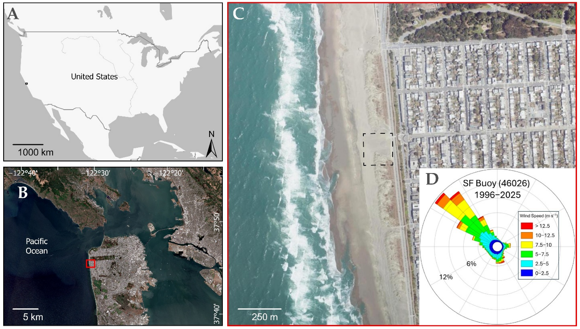
Figure 1. (A) The location of the San Francisco Bay Area within the United States; (B) the study area within the broader region; (C) the study area with a dashed border at Ocean Beach; (D) a wind rose for San Francisco Buoy (NDBC Station 46026), located 33 km offshore. Aerial imagery is from Sentinel-2 (B) and the National Agriculture Imagery Program (FSA) (C).
Remotesensing 18 02998 g001
Figure 2. (A) Shows a section of the source grass harvest area with both (B) nonnative Ammophila arenaria grass, the dominant grass near the study site, and (C) native Leymus mollis, the grass transplanted as part of the revegetation project.
Remotesensing 18 02998 g002
Figure 3. The KAP survey components shown in the image on the left are (A) the Delta kite, (B) Picavet suspension cross, fasteners, and line, (C) camera box, and (D) Canon camera.
Remotesensing 18 02998 g003
Figure 4. Ground control points. (A) Study site with the locations of the October GCPs (red and green), showing the subsection of targets used as checkpoints (green) to test horizontal accuracy; (B) dune surface with a visible target as captured from the kite; (C) 0.6 × 0.6 m target used for GCPs.
Remotesensing 18 02998 g004
Figure 5. Screenshots of Pix4Dmapper ray cloud views, in which each green sphere is an individual photograph taken from the kite (A) or UAV (B), and the location and angle from which it was taken, illustrating the contrasting variable KAP flight compared with the tightly organized, automated path of traditional UAVs.
Remotesensing 18 02998 g005
Figure 6. Data processing and analysis workflow showing core inputs and outputs for KAP-SfM data processing, spatially variable error modeling, and GCD analysis [40].
Remotesensing 18 02998 g006
Figure 7. Spatially variable error inputs and raster surface for the March survey: (A) point cloud density and (B) roughness to create (C) elevation uncertainty (spatially variable error raster)—probabilistic 95% CI. The units are points per square meter (A) and meters (B,C).
Remotesensing 18 02998 g007
Figure 8. Fuzzy categories for FIS model. Bounds of low, medium, and high categories for inputs are centered at tertile splits derived for the most accurate KAP survey, in October 2025.
Remotesensing 18 02998 g008
Figure 9. Estimates of aeolian sand transport rates as a function of wind speed applied to the study site, with C = 1.8 and z0 = 0.0005, as well as variations that include low C = 1.5, high C = 2.1, low z0 = 0.0001, and high z0 = 0.001 using the Bagnold equation (Equation (3)) [40].
Remotesensing 18 02998 g009
Figure 10. Cross-sectional profile: (A) KAP-derived elevation profiles for each of the five surveys along the same transect drawn from west to east; (B) KAP-derived imagery from the October survey with the transect symbolized by a black dotted arrow. The elevation data (A) is unthresholded (raw).
Remotesensing 18 02998 g010
Figure 11. Scattered points accuracy assessment. Points are symbolized for magnitude of random error (absolute value) and labeled by the true value of random error. Point locations were collected via RTK-GNSS on 30 October 2025. Error values are in centimeters; elevation values are in meters above mean sea level.
Remotesensing 18 02998 g011
Figure 12. March to October DoDs: (A) Raw DoD, no error thresholding; (B) DoD with uniform 10 cm minLoD; (C) DoD with uniform 20 cm minLoD; and (D) DoD with spatially variable thresholding based on FIS at 95% CI. Histograms show the volume in cubic meters, with erosion in red and deposition in blue, comparing each of the error models to the raw, unthresholded DoD in grey.
Remotesensing 18 02998 g012
Figure 13. Map of nine 80 m cross-sections spaced 3 m apart, aligned with the 310° prevailing wind at the SF Buoy (see Figure 1), each extending 80 m across the dune/embankment study area. These cross sections are shown over the October imagery with 0.25 m elevation contours, with labeled 1 m index contours, from March (red) and October (black). Cross sections aligned with wind directions interpreted from sand shadows of 290°, 270°, 260° and 280° for Mar, Jun, Aug and Oct, respectively, were also produced and used for alternative estimates of downwind sand transport.
Remotesensing 18 02998 g013
Figure 14. Means of 9 thresholded DoD NW (310°) to SE (130°) cross-sections for 4 periods, based on the 310° prevailing wind at the SF Buoy.
Remotesensing 18 02998 g014
Figure 15. Daily total sand transport rates estimated for Ocean Beach for both 2025 and the long-term record based on the Bagnold equation (Equation (3)) [40], applied to wind data from the San Francisco Buoy (NDBC Station 46026). Kite survey dates are indicated by the vertical green bars.
Remotesensing 18 02998 g015
Table 1. Ground sampling distance, camera height, area covered, number of images, total number of GCPs and checkpoints, and associated vertical RMSE for the five KAP surveys.
KAP SurveyJanuaryMarchJuneAugustOctober
Avg Ground Sampling Distance (m)0.02830.03000.02830.01530.0231
Derived Avg Camera Height (m)83.388.383.345.068.0
Area Covered by Survey (km2)0.0590.0690.0420.0300.046
Number of Images207517173422316
Total Number of GCPs99121112
RMSE (z) GCPs (m)0.0210.0140.0300.0310.022
Checkpoints44455
RMSE (z) Checkpoints (m)0.0320.0160.0430.0410.025
Table 2. FIS rules, using fuzzy classification shown in Figure 8. The inputs are point density and local roughness, and the output is spatially variable uncertainty. In general, lower point density and higher roughness increase elevation uncertainty, and this uncertainty is used to define a spatially variable DoD threshold.
Point DensityRoughnessElevation Uncertainty
LowLowMedium
LowMediumMedium
LowHighHigh
MediumLowLow
MediumMediumMedium
MediumHighHigh
HighLow Low
HighMediumLow
HighHighMedium
Table 3. Vertical error (cm) in independent accuracy assessments. The June accuracy assessment used transects and October used scattered points. The RMSE values are included here for comparison and were generated during photogrammetric processing in during DEM generation; they were not derived from the independent accuracy assessment ground surveys. Number of samples refers to the number of point locations surveyed for comparison with KAP-derived elevation values.
JuneOctober
Systematic Bias−1.783−0.625
Random Error Mean (Absolute Value)4.5022.884
Random Error Median (Absolute Value)3.8112.370
Random Error Standard Deviation (Absolute Value)3.3851.769
Random Error Range (Absolute Value)0.044, 13.5960.274, 8.462
Random Error Range−13.596, 12.345−5.485, 8.462
Number of Samples4639
Pix4Dmapper-reported RMSE of GCPs3.02.2
Table 4. Geomorphic change results for the clipped area between March and October 2025 based on different error analysis: none, uniform minimum level of detection, and spatially variable error based on fuzzy logic. All values are in cubic meters.
Erosion (m3)Deposition (m3)Net Change (m3)
No Uncertainty Analysis (Raw)−1197.991807.25609.26
10 cm minLoD−1095.301786.92691.62
20 cm minLoD−819.291753.94934.66
Spatially Variable Error—80% CI−1187.151799.96612.81
Spatially Variable Error—95% CI−1173.391793.68620.292
Table 5. Geomorphic change results for the clipped area between each survey by raw DEM differencing and probabilistic spatially variable error based on fuzzy logic. The table also includes October–June (marked with *) because August had lower coverage on the eastern edge of the study site.
Erosion (m3)Deposition (m3)Net Change (m3)
No Uncertainty Analysis (Raw)
March–January−530.39770.30239.91
June–March−1192.271398.00205.74
August–June−385.01613.35228.35
* October–June−312.14715.66403.52
October–August−166.57341.74175.17
Spatially Variable Error: FIS (95% Confidence Interval)
March–January−365.04629.60264.56
June–March−1047.631347.42299.79
August–June−181.12470.11288.99
* October–June −147.27572.36425.09
October–August−92.26205.71113.45
Table 6. Modeled wind-driven sand mass transportation rates compared with downwind sand mass accumulation rates, from mean cell rates of sand accumulation and that crossing the 1 m unit width of cross sections and deposited throughout the cross section, a cross section rate. Accumulation cells are those with net positive values of DoD. Units are in kg m−1 d−1. Downwind azimuths are derived from both the SF Buoy 310° prevailing wind and alternatively from measurements of sand shadows on end-month KAP orthoimagery collected in this study. Comparing mean cell rates for the 310° cross sections to wind model rates produced an R2 of 0.99, with 0.96 for the cross section rate.
DoD PeriodWind Model RateMean Cell RatestdCross Section RatestdWind AzimuthMean Cell RatestdCross Section Ratestd
Wind azimuth sourceUsing 310° prevailing wind at SF Buoy Using wind azimuths interpreted from sand shadows in orthoimagery
March–January183.005.060.85120.0944.87290°3.931.5086.8232.02
June–March378.1015.223.18415.0430.95270°14.961.23301.0312.02
August–June321.4011.471.29270.8649.62260°11.712.21195.8719.35
October–August159.703.640.73102.2230.13280°4.061.4487.9619.35
Disclaimer/Publisher’s Note: The statements, opinions and data contained in all publications are solely those of the individual author(s) and contributor(s) and not of MDPI and/or the editor(s). MDPI and/or the editor(s) disclaim responsibility for any injury to people or property resulting from any ideas, methods, instructions or products referred to in the content.