Model-Based Multiframe Radiometric Spatial Reconstruction for Optical Satellite Video

Highlights

What are the main findings?

• A model-based radiometric and spatial reconstruction framework is proposed for short optical satellite video sequences.
• The method jointly incorporates multiframe data fidelity, effective blur modeling, intensity consistency, and spatial regularization.

What are the implications of the main findings?

• Controlled experiments with known HR references show a measurable benefit from retaining sampling phases explicitly in the forward model.
• Real-data results after registration to a common grid are interpreted as multiframe restoration, while static observation weighting shows scene-dependent effects.

Abstract

Satellite video provides repeated observations of the same ground scene within short acquisition intervals, but blur, detector sampling, radiometric differences, noise, and registration errors complicate joint reconstruction. This study presents mixed sparse representation-based collaborative quality improvement (MSR-CQI), a model-based method for joint radiometric and spatial reconstruction of short optical satellite video sequences. The method combines multiframe fidelity, effective PSF modeling, an intensity prior, overlapping group sparsity, high-order nonconvex regularization, intensity bounds, and optional static observation weighting. In controlled ×2 experiments with known HR references, MSR-CQI achieved 42.8714 dB PSNR and 0.9756 SSIM. With the same seven input frames, it achieved 43.1049 dB/0.9714, compared with 42.1369 dB/0.9698 for PnP-NLM and 38.1675 dB/0.9404 for DUF-16L. Retaining measured sampling shifts in the observation operators yielded 45.7461 dB/0.98046, versus 45.0380 dB/0.97904 after LR registration and resampling. The proxy derived from the reserved real frames instead favored the common-grid reconstruction, showing that agreement with this proxy does not establish recovery beyond the native sensor resolution. Static observation weighting was also scene-dependent. These results support retaining sampling phases explicitly in controlled spatial SR, while the real-data results after common-grid resampling are interpreted as multiframe restoration and proxy agreement.

1. Introduction

Satellite video repeatedly observes the same ground area within a short acquisition interval. Compared with conventional multitemporal remote-sensing imagery, adjacent video frames usually contain limited scene change together with small subpixel displacements and local appearance differences [1,2,3,4,5]. When scene content remains approximately stable, these differences provide complementary spatial samples that are unavailable from a single frame. This is the basis of classical multiframe super-resolution (SR), in which several low-resolution (LR) observations are combined to recover finer spatial detail [6,7].

Practical satellite video reconstruction is more difficult because several degradation processes act at the same time. Spatial resolution, image sharpness, and signal-to-noise ratio are closely related in very-high-resolution satellite imagery [8]. Optical blur, detector sampling, noise, and residual registration errors further constrain multiframe reconstruction. Simply increasing the number of input frames therefore does not guarantee better reconstruction. Poorly aligned or locally inconsistent observations may instead introduce bias, blurred boundaries, or duplicated structures into the reconstructed image.

Multiframe information has been widely used in satellite video and remote sensing reconstruction [2,3,4,5,9]. Recent studies have improved reconstruction through frequency-domain processing, multiscale integration of spatial and temporal information, long-range spatial representation, and explicit treatment of image degradation [5,10,11,12,13,14,15]. Variational methods that combine observation models with image priors have also been investigated for remote sensing super-resolution [16]. Although these studies have improved spatial detail recovery and temporal alignment, blur variation, intensity differences among frames, observation weighting, and spatial regularization are less often considered together within one inverse formulation.

Satellite video restoration commonly involves registration, intensity correction, denoising, and spatial reconstruction. Residual errors introduced during these operations may affect the final HR estimate, particularly when the observations differ in registration accuracy, intensity consistency, or spatial degradation. This motivates a joint formulation in which the contributions of individual frames and spatial constraints are considered within the reconstruction model.

Radiometric enhancement and exposure-fusion methods provide useful ideas for handling unequal intensity information [17,18,19], but their assumptions do not directly match the satellite video setting considered here. Conventional HDR methods often rely on multiple exposure settings, camera-response estimation, or explicit exposure fusion. In contrast, the short satellite video bursts used in this study are acquired under fixed or nearly fixed imaging conditions. We therefore do not estimate physical exposure parameters or a camera-response curve. The reconstruction is performed in the normalized digital-intensity domain, and the output should not be interpreted as calibrated radiance or reflectance.

Based on these considerations, we formulate satellite video restoration as a model-based radiometric and spatial inverse problem and develop a mixed sparse representation-based collaborative quality improvement framework, termed MSR-CQI. The method operates on registered and per-channel normalized LR observations. It combines multiframe fidelity, an effective blur model, a weak intensity prior, overlapping-group sparsity, high-order regularization, and intensity constraints. Static observation weights derived from valid support, normalized intensity range, and post-registration temporal consistency are included as an optional component and are examined through direct comparison with uniform observation weighting rather than assumed to be uniformly beneficial. The resulting objective is optimized using the alternating direction method of multipliers (ADMM).

The main contributions of this study are threefold. First, we formulate normalized satellite video reconstruction as a unified inverse problem that combines multiframe observation fidelity, effective blur and sampling, a weak intensity constraint, spatial regularization, and bounded intensity. Second, we provide an operator-based ADMM solution that decomposes the reconstruction into data-consistency, grouped-sparsity, high-order regularization, and intensity-projection subproblems. Third, we evaluate the formulation using controlled experiments with known HR references, analysis of real sequences after registration to a common grid, component analysis, and controlled sensitivity experiments, and characterize the effects of inter-frame inconsistency and static observation weighting.

The experiments focus on short satellite video sequences with limited structural change. Controlled ×2 experiments retain known subpixel sampling phases and use independent HR references. In the real-data pathway, frames are resampled to a common LR grid before reconstruction; these experiments are therefore interpreted as multiframe restoration with ×2 reconstruction after registration and resampling to a common LR grid. Reserved frames provide only proxy references for relative consistency analysis and are not treated as independent HR ground truth.

The remainder of this paper is organized as follows. Section 2 describes the datasets, observation model, radiometric and spatial reconstruction framework, optimization procedure, and evaluation protocol. Section 3 presents the analysis of the real sequences, comparisons using known HR references, component analysis, sensitivity experiments, and computational analysis.

2. Materials and Methods

Satellite video restoration is formulated as a joint radiometric and spatial reconstruction problem in which consecutive frames are treated as degraded observations of a common latent image.

Blur, undersampling, noise, radiometric variation, and inter-frame differences are considered jointly. MSR-CQI combines multiframe information, a weak intensity constraint, OGS and high-order regularization, and intensity-bounds projection. Optional static observation weights are estimated from valid support, normalized intensity range, and temporal consistency after registration. Because the real frames are first registered and resampled to a common LR grid, the principal real-data pathway is interpreted as multiframe radiometric and spatial restoration rather than direct acquisition-phase super-resolution.

2.1. Satellite Video Datasets and Experimental Frame Protocol

Three satellite video datasets comprising four test sequences were used: OVS-1A, Jilin-1, and two regions of interest (ROIs) from Luojia03-01. For each sequence, reconstruction frames, reserved evaluation frames, and a registration reference frame were specified before reconstruction.

The OVS-1A sequence was acquired over Damascus, Syria, on 19 June 2017. The sensor records nominal 10-bit video at 20 fps, with a reported multispectral ground sampling distance (GSD) of approximately 1.98 m. Nine RGB frames (0030–0038), each 1064 × 1032 pixels, were used. Frames 0030–0036 were used for reconstruction, frames 0037–0038 were reserved for evaluation, and frame 0033 served as the registration reference. After per-channel normalization, translation-based registration, and common-valid cropping, an 800 × 800 LR region was retained.

The Jilin-1 sequence was acquired over Hohhot, Inner Mongolia, China, on 21 September 2020, with an effective frame rate of 10 fps and a GSD of approximately 2.88 m. Ten RGB frames (0143–0152), each 1024 × 1024 pixels, were used. Frames 0143–0150 were used for reconstruction, frames 0151–0152 were reserved for evaluation, and frame 0147 served as the registration reference. The same normalization, registration, and common-valid cropping procedure produced an 800 × 800 LR region.

Luojia03-01 was evaluated using two ROIs acquired at 6 fps, with a nominal nadir GSD of approximately 0.7 m. ROI-1 covers Port Elizabeth, South Africa, and was acquired on 5 April 2024, with a working size of 850 × 1298 pixels. ROI-2 covers Dubai Airport and was acquired on 21 February 2024, with a working size of 871 × 1189 pixels. For both ROIs, frames 1–8 were used for reconstruction, frames 9–10 were reserved for evaluation, and frame 5 served as the registration reference. After registration and common-valid cropping, an 800 × 800 LR region was retained for the principal real sequence evaluation.

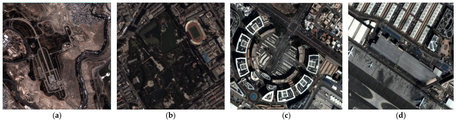
Representative frames from the four sequences are shown in Figure 1. The experiments focus on short image sequences with limited scene change; sensitivity to larger geometric and structural inconsistencies is examined separately in Section 3.6.

2.2. Satellite Video Image Formation Under Coupled Radiometric and Spatial Degradations

Classical multiframe SR similarly represents each LR observation as a geometrically shifted, blurred, and sampled measurement of an underlying HR image [20,21].

To describe the combined spatial and radiometric degradation in satellite video observations, each frame is represented as a degraded measurement of a common latent high-resolution image. The reconstruction is carried out in the normalized digital-intensity domain and does not recover physically calibrated radiance or reflectance. Let $\mathbf{z}$ denote the latent HR image. For the $i$-th frame, the observed LR frame ${\mathit{g}}_i$ is conceptually generated by geometric displacement, effective blur, detector sampling, the sensor-dependent digital response, and additive observation noise:

$${\mathit{g}}_i=f_i{(D_{i}B}_i{M}_i\mathbf{z})+n_i,i=1,2,\dots ,N.$$

(1)

where $M_i$, $B_i$ and $D_i$ denote geometric warping, effective blur, and detector-sampling operators, respectively. The function $f_i(\cdot )$ represents the acquisition-level digital response, $n_i$ denotes additive observation noise, and $N$ is the number of observed frames. Equation (1) is used as a conceptual description of the image-formation process. 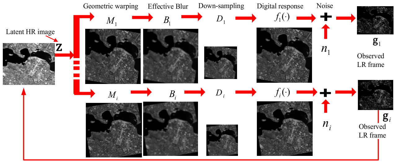The implemented method does not estimate or invert $f_i(\cdot )$, nor does it estimate a physical exposure parameter. The acquisition model and its relation to the implemented reconstruction pathway are illustrated in Figure 2.

Before reconstruction, each RGB channel is normalized using scaling factors determined exclusively from the reconstruction frames. For the principal real-data pathway, the observations are first interpolated onto the designated LR reference grid and cropped to common valid support. The resulting normalized LR observation is denoted by $y_i$, and the working model is written as

$$y_i=A_i\mathbf{z}+{\tilde{n}}_i,A_i=D_i{B}_i{M}_i,$$

Because geometric displacement has already been compensated during registration and resampling, the residual geometric operator is set to $M_i=I$ for the common-grid reconstruction. This resampling step does not explicitly retain the original detector-grid sampling locations within the subsequent inverse operator. The principal real-data pathway is therefore interpreted as multiframe radiometric and spatial restoration with regularized ×2 reconstruction on a common LR grid.

In the controlled experiments with known HR references, prescribed subpixel shifts are retained explicitly in the forward operators. A separate paired Jilin-1 experiment also retains the measured translations within $A_i$ without LR pre-registration. These experiments examine the effect of retaining the sampling shifts explicitly in the observation model.

The blur term is represented by an effective discrete point-spread function (PSF) rather than by a sensor-specific modulation transfer function. The prescribed degradation kernel is used in the controlled experiments. For the real satellite video sequences, four PSF forms were considered: Identity 1 × 1, Gaussian 3 × 3 ($\sigma =0.8$), Gaussian 5 × 5 ($\sigma =1.0$), and Gaussian 7 × 7 ($\sigma =1.2$). The procedure used to determine the effective PSF for the real sequences is described in Section 2.6.

The formulation assumes that scene structure remains approximately stable within each short satellite video sequence. Residual registration error, occlusion, local parallax around elevated structures, and persistent target motion may introduce ghosting, duplicated edges, or local radiometric deviations. Their effects are evaluated separately in the controlled sensitivity experiments.

2.3. Unified Radiometric and Spatial Reconstruction Model

Starting from the normalized observation model in Section 2.2, MSR-CQI estimates the latent HR image using multiframe observations, a weak intensity prior, first-order grouped sparsity, high-order regularization, and an intensity-range constraint. The formulation permits diagonal observation weights; the uniform-weight case is included explicitly in the component analysis. The reconstruction problem is formulated as

$${\mathrm{m}\mathrm{i}\mathrm{n}}_{\mathbf{z}}{\displaystyle \frac{\lambda }{2}}{\displaystyle {\sum }_{i=1}^N}{∥{\mathsf{\Omega }}_i^{{\displaystyle \frac{1}{2}}}\left(A_i\mathbf{z}-{\mathbf{y}}_i\right)∥}_2^2+{\displaystyle \frac{\eta }{2}}{∥{\mathsf{\Omega }}_0^{{\displaystyle \frac{1}{2}}}\left(\mathbf{z}-{\mathbf{z}}_{\mathrm{p}\mathrm{r}\mathrm{e}}\right)∥}_2^2+\alpha {\Phi }_{\mathrm{O}\mathrm{G}\mathrm{S}}\left(\nabla \mathbf{z}\right)+\beta {∥{\nabla }^2\mathbf{z}∥}_p^p+{\iota }_{\mathcal{C}}\left(\mathbf{z}\right),$$

(2)

where $\mathbf{z}\in {\mathbb{R}}^M$ is the vectorized HR image containing $M$ pixels, whereas ${\mathbf{y}}_i\in {\mathbb{R}}^m$ denotes the $i$-th registered normalized LR observation with m pixels. The operator ${\mathbf{A}}_i\in {\mathbb{R}}^{m\times M}$ maps the HR image to the LR observation domain. The diagonal matrix ${\mathsf{\Omega }}_i=\mathrm{D}\mathrm{i}\mathrm{a}\mathrm{g}\left({\mathbf{q}}_i\right)\in {\mathbb{R}}^{m\times m}$ weights the data fidelity of frame $i$, whereas ${\mathsf{\Omega }}_0=\mathrm{D}\mathrm{i}\mathrm{a}\mathrm{g}\left({\mathsf{\omega }}_0\right)\in {\mathbb{R}}^{M\times M}$ controls the spatial contribution of the preliminary estimate ${\mathbf{z}}_{\mathrm{p}\mathrm{r}\mathrm{e}}$. Both weighting matrices are computed before optimization and remain unchanged during each ADMM run; their construction is given in Section 2.5.

The parameters $\lambda$, $\eta$, $\alpha$, and $\beta$ control the multiframe fidelity, weak intensity prior, OGS regularization, and high-order regularization, respectively. The exponent $0<p<1$ introduces a nonconvex sparsity penalty on the second-order response,

$$\parallel {\nabla }^2\mathbf{z}{\parallel }_p^p={\displaystyle {\sum }_{j=1}^M} |({\nabla }^2\mathbf{z}{)}_j{|}^p.$$

The operator $\nabla$ is the periodic first-order forward difference used in the implementation, and ${\nabla }^2={\nabla }^{\mathrm{T}}\nabla$ denotes the corresponding positive periodic Laplacian.

The first-order regularizer acts on overlapping neighborhoods of the gradient field. Its penalty is defined by

$${\mathsf{\Phi }}_{\mathrm{O}\mathrm{G}\mathrm{S}}(\mathbf{v})={\sum }_x {[{\sum }_{r\in {\mathcal{G}}_x} \parallel \mathbf{v}(r){\parallel }_2^2+ {ϵ}_{\mathrm{O}\mathrm{G}\mathrm{S}}]}^{1/2},$$

where ${\mathcal{G}}_x$ denotes the 3 × 3 overlapping neighborhood centered at pixel $x$, $\mathbf{v}\left(r\right)$ denotes the local first-order gradient vector, and ${ϵ}_{\mathrm{O}\mathrm{G}\mathrm{S}}={10}^{-6}$ provides numerical stabilization in the majorization-minimization update.

The reconstructed normalized intensity is restricted elementwise to [0, 1]. The feasible set is therefore

$$C=\{\mathbf{z}\in {\mathbb{R}}^M\mid 0\le {\mathbf{z}}_j\le 1, j=1,\dots ,M\}.$$

Its indicator function is

$${\iota }_{\mathcal{C}}(\mathsf{\xi })=\left\{\begin{array}{c}0,\mathbf{\xi }\in \mathcal{C},\\ +\infty ,\mathbf{\xi }\notin \mathcal{C}.\end{array}\right.$$

(3)

A relatively small weight is assigned to the intensity prior in the reported experiments, with $\eta /\lambda =0.001.$

To separate the nonsmooth terms, three auxiliary variables are introduced:

$$\mathbf{v}=\nabla \mathbf{z},\mathbf{w}={\nabla }^2\mathbf{z},\mathbf{u}=\mathbf{z}.$$

Using the auxiliary variables and the indicator function defined in Equation (3), Equation (2) can be rewritten as

$$\begin{gathered} \underset{\mathbf{z},\mathbf{v},\mathbf{w},\mathbf{u}}{\min }{\displaystyle \frac{\lambda }{2}}{\displaystyle \sum _{i=1}^N}{∥{\mathsf{\Omega }}_i^{1/2}\left(A_i\mathbf{z}-y_i\right)∥}_2^2+{\displaystyle \frac{\eta }{2}}{∥{\mathsf{\Omega }}_0^{1/2}\left(\mathbf{z}-{\mathbf{z}}_{\mathrm{p}\mathrm{r}\mathrm{e}}\right)∥}_2^2 \\ +\alpha {\Phi }_{\mathrm{O}\mathrm{G}\mathrm{S}}\left(\mathbf{v}\right)+\beta {∥w∥}_p^p+{\iota }_{\mathcal{C}}\left(\mathbf{u}\right), \\ \mathrm{s}.\mathrm{t}.\mathbf{v}=\nabla \mathbf{z}, \mathbf{w}={\nabla }^2\mathbf{z}, \mathbf{u}=\mathbf{z}. \end{gathered}$$

(4)

Equation (4) is solved using the alternating direction method of multipliers (ADMM) [22]. With scaled dual variables $d_1$, $d_2$, and $d_3$, the scaled augmented-Lagrangian expression, up to additive constants independent of the primal variables, is

$$\begin{gathered} L_{\rho }\left(\mathbf{z},\mathbf{v},\mathbf{w},\mathbf{u};d_1,d_2,d_3\right)={\displaystyle \frac{\lambda }{2}}{\displaystyle \sum _{i=1}^N}{∥{\mathsf{\Omega }}_i^{1/2}\left(A_i\mathbf{z}-y_i\right)∥}_2^2+{\displaystyle \frac{\eta }{2}}{∥{\mathsf{\Omega }}_0^{1/2}\left(\mathbf{z}-{\mathbf{z}}_{\mathrm{p}\mathrm{r}\mathrm{e}}\right)∥}_2^2 \\ +\alpha {\Phi }_{\mathrm{O}\mathrm{G}\mathrm{S}}\left(\mathbf{v}\right)+\beta {∥\mathbf{w}∥}_p^p+{\iota }_{\mathcal{C}}\left(\mathbf{u}\right) \\ +{\displaystyle \frac{{\rho }_1}{2}}{∥\nabla \mathbf{z}-\mathbf{v}+d_1∥}_2^2+{\displaystyle \frac{{\rho }_2}{2}}{\parallel {\nabla }^2\mathbf{z}-\mathbf{w}+d_2\parallel }_2^2+{\displaystyle \frac{{\rho }_3}{2}}{∥\mathbf{z}-\mathbf{u}+d_3∥}_2^2 \end{gathered}$$

(5)

In Equation (5), the positive penalties ${\rho }_1$, ${\rho }_2$, and ${\rho }_3$ correspond to the first-order splitting, high-order splitting, and intensity bounds constraint, respectively. This variable decomposition isolates the quadratic reconstruction step from the OGS, nonconvex high-order, and projection updates.

2.4. ADMM-Based Optimization for Unified Reconstruction

The optimization alternates between the latent HR image and the three auxiliary variables, followed by updates of the scaled dual variables. The static observation weight matrices used in Equations (2) and (4)–(7) are obtained from the registered normalized observations before optimization and are not recomputed from the ADMM residuals.

(1) 

Update of $\mathbf{z}$

With $\mathbf{v}$, $\mathbf{w}$ and $\mathbf{u}$ fixed at iteration k, the latent image is updated by solving

$$\begin{gathered} {\mathbf{z}}^{k+1}=\mathrm{a}\mathrm{r}\mathrm{g}\underset{z}{\mathrm{m}\mathrm{i}\mathrm{n}}{\displaystyle \frac{\lambda }{2}}{\displaystyle \sum _{i=1}^N}{∥{\mathsf{\Omega }}_i^{1/2}\left(A_i\mathbf{z}-{\mathbf{y}}_i\right)∥}_2^2+{\displaystyle \frac{\eta }{2}}{∥{\mathsf{\Omega }}_0^{1/2}\left(\mathbf{z}-{\mathbf{z}}_{\mathrm{p}\mathrm{r}\mathrm{e}}\right)∥}_2^2 \\ +{\displaystyle \frac{{\rho }_1}{2}}{∥\nabla \mathbf{z}-{\mathbf{v}}^k+d_1^k∥}_2^2+{\displaystyle \frac{{\rho }_2}{2}}{∥{\nabla }^2\mathbf{z}-{\mathbf{w}}^k+d_2^k∥}_2^2+{\displaystyle \frac{{\rho }_3}{2}}{∥\mathbf{z}-{\mathbf{u}}^k+d_3^k∥}_2^2 \end{gathered}$$

(6)

Taking the derivative of Equation (6) with respect to z and setting it to zero gives

$$\begin{gathered} \left(\lambda {\displaystyle \sum _{i=1}^N}{A}_i^T{\mathsf{\Omega }}_i{A}_i+\eta {\mathsf{\Omega }}_0+{\rho }_1{\nabla }^T\nabla +{\rho }_2{\left({\nabla }^2\right)}^T{\nabla }^2+{\rho }_{3}I\right){\mathbf{z}}^{k+1} \\ =\lambda {\displaystyle {\sum }_{i=1}^N}{A}_i^T{\mathsf{\Omega }}_i{y}_i+\eta {\mathsf{\Omega }}_0{\mathbf{z}}_{\mathrm{p}\mathrm{r}\mathrm{e}}+{\rho }_1{\nabla }^T\left({\mathbf{v}}^k-d_1^k\right)+{\rho }_2{\left({\nabla }^2\right)}^T\left({\mathbf{w}}^k-d_2^k\right)+{\rho }_3\left({\mathbf{u}}^k-d_3^k\right), \end{gathered}$$

(7)

where $I$ is the identity matrix. Because ${\mathsf{\Omega }}_i$ and ${\mathsf{\Omega }}_0$ are diagonal nonnegative matrices and ${\rho }_3>0$, the coefficient matrix in Equation (7) is symmetric positive definite. The $\mathbf{z}$-subproblem therefore has a unique solution and is suitable for conjugate-gradient iteration.

Equation (7) is solved using MATLAB’s pcg routine without an explicit preconditioner. The relative tolerance is 10⁻⁴, and the maximum number of inner iterations is 30. Blur is represented by linear convolution. Warping and sampling remain linear operators in the general formulation, while the residual warping operator is set to the identity for the registered real-data inputs.

(2) 

Update of $\mathbf{v}$

The first-order auxiliary variable is obtained from

$${\mathbf{v}}^{k+1}=\mathrm{a}\mathrm{r}\mathrm{g}\underset{\mathbf{v}}{\mathrm{m}\mathrm{i}\mathrm{n}}\alpha {\Phi }_{\mathrm{O}\mathrm{G}\mathrm{S}}\left(\mathbf{v}\right)+{\displaystyle \frac{{\rho }_1}{2}}{∥\mathbf{v}-q_{\mathbf{v}}^k∥}_2^2, q_{\mathbf{v}}^k=\nabla {\mathbf{z}}^{k+1}+d_1^k.$$

(8)

The overlapping-group penalty follows the OGS formulation in [23], while its inner update is implemented using a majorization-minimization strategy consistent with [24]. The update acts on overlapping gradient neighborhoods rather than applying independent shrinkage to individual pixels. The number of inner MM iterations is fixed as specified in Section 2.7.

(3) 

Update of $\mathbf{w}$

With $\mathbf{z}$, $\mathbf{v}$, and $\mathbf{u}$ fixed, the $\mathbf{w}$-subproblem is

$${\mathbf{w}}^{k+1}=\underset{\mathbf{w}}{\mathrm{a}\mathrm{r}\mathrm{g}\mathrm{m}\mathrm{i}\mathrm{n}}\beta \parallel \mathbf{w}{\parallel }_p^p+ {\displaystyle \frac{{\rho }_2}{2}}\parallel \mathbf{w}-{\mathbf{q}}_w^k{\parallel }_2^2, {\mathbf{q}}_w^k={\nabla }^2{\mathbf{z}}^{k+1}+d_2^k.$$

(9)

Since $0<p<1$, the ${\mathcal{l}}_p$ term is nonconvex. An iterative reweighted ${\mathcal{l}}_1$ surrogate is therefore used [25]. At iteration k, the elementwise weight is

$${\theta }_j^k=\beta p{\left(\left|w_j^k\right|+\zeta \right)}^{p-1},\zeta >0.$$

(10)

The corresponding surrogate becomes

$${\mathbf{w}}^{k+1}=\mathrm{a}\mathrm{r}\mathrm{g}\underset{\mathbf{w}}{\mathrm{m}\mathrm{i}\mathrm{n}} {\displaystyle \frac{{\rho }_2}{2}}{∥\mathbf{w}-{\mathbf{q}}_w^k∥}_2^2+{\sum }_j {\theta }_j^k|{\mathbf{w}}_j|.$$

(11)

For fixed ${\theta }^k$, Equation (11) is convex and separable. Its minimizer is obtained by elementwise soft thresholding:

$${\mathbf{w}}^{k+1}=\mathrm{s}\mathrm{o}\mathrm{f}\mathrm{t}({\mathbf{q}}_{\mathrm{w}}^k,{\displaystyle \frac{{\theta }^k}{{\rho }_2}}),$$

(12)

where

$$\mathrm{s}\mathrm{o}\mathrm{f}\mathrm{t}(\mathbf{q},\tau )=\mathrm{s}\mathrm{i}\mathrm{g}\mathrm{n}\left(\mathbf{q}\right)\odot max\left(\right|\mathbf{q}|-\tau ,0).$$

(13)

Here $\odot$, $\mid \cdot \mid$ and $\mathrm{m}\mathrm{a}\mathrm{x}(\cdot ,0)$ are applied elementwise. The small constant $\zeta$ prevents singular weights when the current high-order coefficient approaches zero.

(4) 

Update of $\mathbf{u}$

The variable $\mathbf{u}$ enforces the intensity bounds:

$${\mathbf{u}}^{k+1}=\underset{\mathbf{u}}{\mathrm{a}\mathrm{r}\mathrm{g}\mathrm{m}\mathrm{i}\mathrm{n}}{\iota }_{\mathcal{C}}\left(\mathbf{u}\right)+{\displaystyle \frac{{\rho }_3}{2}}\parallel \mathbf{u}-{\mathbf{q}}_u^k{\parallel }_2^2, {\mathbf{q}}_u^k={\mathbf{z}}^{k+1}+d_3^k.$$

(14)

This subproblem is the Euclidean projection onto $\mathcal{C}$:

$${\mathbf{u}}^{k+1}={\mathsf{\Pi }}_{\mathcal{C}}\left({\mathbf{q}}_{\mathbf{u}}^k\right)=min\left(max\right({\mathbf{q}}_{\mathbf{u}}^k,0),1).$$

(15)

where ${\mathsf{\Pi }}_{\mathcal{C}}(\cdot )$ denotes projection onto the feasible set $\mathcal{C}=\{\mathbf{u}\in {\mathbb{R}}^M:0\le u_j\le 1\}$, which reduces to elementwise clipping.

(5) 

Scaled dual-variable updates

After updating $\mathbf{z}$, $\mathbf{v}$, $\mathbf{w}$, and $\mathbf{u}$, the scaled dual variables are updated as

$$d_1^{k+1}=d_1^k+\nabla {\mathbf{z}}^{k+1}-{\mathbf{v}}^{k+1},$$

(16)

$$d_2^{k+1}=d_2^k+{\nabla }^2{\mathbf{z}}^{k+1}-{\mathbf{w}}^{k+1},$$

(17)

$$d_3^{k+1}=d_3^k+{\mathbf{z}}^{k+1}-{\mathbf{u}}^{k+1}.$$

(18)

For the experiments reported in this study, the solver uses a fixed budget of K_max = 30 ADMM iterations. Relative iterate change together with the primal and dual residuals is recorded for numerical diagnosis but is not used for early termination. This fixed iteration budget keeps the computational setting identical across the reported component analyses.

Because the objective contains a nonconvex ${\mathcal{l}}_p$ term and the OGS subproblem is solved using a finite number of MM iterations, convergence behavior is evaluated numerically using the objective value and primal and dual residuals.

2.5. Static Observation Weighting and Normalized Intensity Prior

Static observation weights are derived from the registered and normalized LR observations before ADMM optimization. For each frame, a pixelwise weight map $q_i$ modulates the data-fidelity term, while an HR weight map ${\mathit{\omega }}_0$ controls the spatial contribution of the preliminary estimate. These quantities are computed once before reconstruction and remain unchanged during optimization. Because the influence of static weighting varies among scenes, the uniform-weight case is retained as a direct comparison.

Let $y_i\left(x\right)\in \left[0,1\right]$ denote the normalized intensity at pixel $x$ in frame $i$, and let $m_i\left(x\right)\in \{0,1\}$ indicate valid support. The temporal median over valid observations and the corresponding residual are defined as

$$y_{\mathrm{m}\mathrm{e}\mathrm{d}}\left(x\right)={\mathrm{m}\mathrm{e}\mathrm{d}\mathrm{i}\mathrm{a}\mathrm{n}}_{i:m_i\left(x\right)=1}{y}_i\left(x\right), r_i\left(x\right)=y_i\left(x\right)-y_{\mathrm{m}\mathrm{e}\mathrm{d}}\left(x\right).$$

(19)

A robust residual scale is then estimated from the valid observations. Defining

$$\overline{r}={\mathrm{m}\mathrm{e}\mathrm{d}\mathrm{i}\mathrm{a}\mathrm{n}}_{(j,x^{\prime }):m_j(x^{\prime })=1}{r}_j(x^{\prime }).$$

gives

$${\sigma }_{\mathrm{r}\mathrm{e}\mathrm{g}}=1.4826{\mathrm{m}\mathrm{e}\mathrm{d}\mathrm{i}\mathrm{a}\mathrm{n}}_{(i,x):m_i\left(x\right)=1}\left|r_i\right(x)-\overline{r}|+{10}^{-6}.$$

(20)

To reduce the contribution of normalized intensities close to the lower and upper bounds, an intensity-range weighting term is defined as

$$c_{\mathrm{i}\mathrm{n}\mathrm{t},i}(x)=\mathrm{c}\mathrm{l}\mathrm{i}\mathrm{p}\left[\mathrm{e}\mathrm{x}\mathrm{p}\left(-{\displaystyle \frac{{\left(y_i\left(x\right)-0.5\right)}^2}{2{\sigma }_{\mathrm{i}\mathrm{n}\mathrm{t}}^2}}\right),{\omega }_{min},1\right].$$

(21)

This term is defined solely in the normalized digital-intensity domain. It does not use sensor exposure time, gain, full-well capacity, radiometric calibration, saturation thresholds, or a calibrated noise model, and therefore should not be interpreted as a physical exposure or sensor-reliability measure. The clipping operator is defined as

$$\mathrm{c}\mathrm{l}\mathrm{i}\mathrm{p}(a,l,u)=min\left\{max\right(a,l),u\}$$

Temporal consistency after registration is measured by

$$c_{\mathrm{t}\mathrm{c},i}(x)=\mathrm{c}\mathrm{l}\mathrm{i}\mathrm{p}\left[\mathrm{e}\mathrm{x}\mathrm{p}\left(-{\displaystyle \frac{1}{2}}{\left({\displaystyle \frac{r_i\left(x\right)}{{\sigma }_{\mathrm{r}\mathrm{e}\mathrm{g}}}}\right)}^2\right),{\omega }_{\mathrm{m}\mathrm{i}\mathrm{n}},1\right].$$

(22)

Pixelwise disagreement across frames is summarized by

$$MA{D}_t\left(x\right)={\mathrm{m}\mathrm{e}\mathrm{d}\mathrm{i}\mathrm{a}\mathrm{n}}_{i:m_i\left(x\right)=1}\left|y_i\right(x)-y_{\mathrm{m}\mathrm{e}\mathrm{d}}(x\left)\right|.$$

(23)

and converted to an agreement factor:

$$c_{\mathrm{a}\mathrm{g}\mathrm{r}}(x)=\mathrm{c}\mathrm{l}\mathrm{i}\mathrm{p}\left[\mathrm{e}\mathrm{x}\mathrm{p}\left(-{\displaystyle \frac{1}{2}}{\left({\displaystyle \frac{{\mathrm{M}\mathrm{A}\mathrm{D}}_t\left(x\right)}{{\sigma }_{\mathrm{r}\mathrm{e}\mathrm{g}}}}\right)}^2\right),{\omega }_{\mathrm{m}\mathrm{i}\mathrm{n}},1\right].$$

(24)

The observation weight is then

$$q_i\left(x\right)=m_i\left(x\right)c_{\mathrm{i}nt,i}\left(x\right)c_{\mathrm{t}\mathrm{c},i}\left(x\right).$$

(25)

and its locally normalized allocation weight is

$$a_i\left(x\right)={\displaystyle \frac{q_i\left(x\right)}{{\displaystyle {\sum }_{j=1}^N}{q}_j\left(x\right)+\epsilon }}.$$

(26)

The preliminary HR estimate and its spatial weight map are

$$z_{\mathrm{p}\mathrm{r}\mathrm{e}}={\mathcal{U}}_{\mathrm{b}\mathrm{i}\mathrm{c}}\left({\displaystyle \sum _{i=1}^N} a_i{y}_i\right),$$

$${\mathsf{\omega }}_0={\mathcal{U}}_{\mathrm{n}\mathrm{n}}\left[\mathrm{c}\mathrm{l}\mathrm{i}\mathrm{p}\left({\displaystyle \frac{1}{N}}{\displaystyle {\sum }_{i=1}^N} q_i{c}_{\mathrm{a}\mathrm{g}\mathrm{r}},{\omega }_{\mathrm{m}\mathrm{i}\mathrm{n}},1\right)\right],{\mathsf{\Omega }}_0=\mathrm{D}\mathrm{i}\mathrm{a}\mathrm{g}\left({\mathsf{\omega }}_0\right).$$

(27)

Here, ${\mathcal{U}}_{\mathrm{b}\mathrm{i}\mathrm{c}}$ and ${\mathcal{U}}_{\mathrm{n}\mathrm{n}}$ denote bicubic and nearest-neighbor upsampling to the HR grid. The reported implementation uses ${\sigma }_{\mathrm{i}nt}=0.25$, ${\omega }_{\mathrm{m}\mathrm{i}\mathrm{n}}=0.02$. The small positive constant $\epsilon$ in Equation (26) prevents division by zero; it is distinct from the 10⁻⁶ stabilization term in Equation (20).

Finally,

$${\Omega }_i=\mathrm{d}\mathrm{i}\mathrm{a}\mathrm{g}\left({\mathbf{q}}_i\right).$$

(28)

Accordingly, ${\mathbf{z}}_{\mathrm{p}\mathrm{r}\mathrm{e}}$ serves as a weak intensity prior, ${\Omega }_0$ controls its spatial contribution, and ${\Omega }_i$ weights observation $i$. None of these weighting quantities is updated from the ADMM residuals.

The ADMM penalty parameters ${\rho }_1$, ${\rho }_2$, and ${\rho }_3$ were selected separately to balance first-order structural consistency, high-order regularization, and bounded intensity projection. In the final implementation, ${\rho }_1=0.35$, ${\rho }_2=0.04$, and ${\rho }_3=0.80$. The implementation details of the proposed method are summarized in Algorithm 1.

Algorithm 1. ADMM solver for the proposed MSR-CQI reconstruction

(1) Initialization: Input: Observed LR RGB frames $\{g_i{\}}_{i=1}^N$; preprocessing registration transforms; PSF set; ×2 sampling operator; parameters $\lambda , \eta , \alpha , \beta , p, {\rho }_1, {\rho }_2, {\rho }_3, {\sigma }_{\mathrm{i}\mathrm{n}\mathrm{t}}, {\omega }_{\mathrm{m}\mathrm{i}\mathrm{n}}$; maximum ADMM iterations $K_{max}=30$. 1. Apply the preprocessing normalization and fixed registration transforms to obtain $y_i$. 2. Determine the effective PSF using the spatially separated protocol described in Section 2.6, and then construct $A_i=D_i{B}_i{M}_i$. For the common-grid reconstruction, set the residual geometric operator to $M_i=I$. For the paired reconstruction on the original sampling grid, retain the measured transformation within $A_i$. 3. Compute ${\mathit{z}}_{\mathrm{p}\mathrm{r}\mathrm{e}}$, $\{{\mathsf{\Omega }}_i{\}}_{i=1}^N$, and ${\mathsf{\Omega }}_0$ according to Equations (19)–(28). 4. Initialize ${\mathbf{z}}^0={\mathbf{z}}_{\mathrm{p}\mathrm{r}\mathrm{e}},{\mathbf{v}}^0=\nabla {\mathbf{z}}^0,{\mathbf{w}}^0={\nabla }^2{\mathbf{z}}^0,{\mathbf{u}}^0={\mathbf{z}}^0,$ and ${\mathbf{d}}_1^0={\mathbf{d}}_2^0={\mathbf{d}}_3^0=\mathbf{0}.$ 5. For $k=0,1,\dots ,K_{max}-1$ do:    (a) Update ${\mathbf{z}}^{k+1}$ by solving Equation (7);    (b) Update ${\mathbf{v}}^{k+1}$ by Equation (8);    (c) Update ${\mathbf{w}}^{k+1}$ by Equations (9)–(13);    (d) Update ${\mathbf{u}}^{k+1}$ by Equations (14) and (15);    (e) Update ${\mathbf{d}}_1^{k+1}$, ${\mathbf{d}}_2^{k+1}$, and ${\mathbf{d}}_3^{k+1}$ by Equations (16)–(18);    (f) Record the relative iterate change and primal/dual residuals. 6. Stop after $K_{max}=30$ ADMM iterations. 7. Output: reconstructed image $\widehat{\mathbf{z}}={\mathbf{z}}^{K_{\mathrm{m}\mathrm{a}\mathrm{x}}}$.

Implementation note: The static observation weight maps are computed from the registered observations before optimization and remain fixed during each ADMM run.

2.6. Evaluation Protocol and Metrics

Native HR reference images are unavailable for the real satellite video sequences. For each sequence, two LR frames reserved from reconstruction were registered, averaged, and bicubically upsampled to provide a common reference for relative comparison. Because this reference is derived entirely from LR observations, it contains no independent HR information and cannot be used to demonstrate spatial-detail recovery beyond the native sensor sampling. PSNR and SSIM calculated against this reference are therefore reported as proxy-agreement metrics and are used only for relative comparison among reconstruction methods. Assessment of spatial reconstruction accuracy relies primarily on the controlled experiments, for which the HR image is known, and the corresponding LR observations are generated under prescribed degradation conditions.

LOE [26] was used to measure changes in relative brightness ordering, whereas VIF [27] was used to evaluate information fidelity relative to the reference image. The same metric implementations and image pairs were used for all compared methods.

The frame assignments specified in Section 2.1 were used unchanged for normalization, reconstruction, proxy construction, and evaluation. Channel normalization was determined from the reconstruction frames and subsequently applied without modification to the reserved frames. OVS-1A digital numbers were normalized by 1023. The Luojia03-01 data were stored in uint16 format but occupied a measured digital-number range of 0–255 and were therefore normalized by 255. Registration transforms were estimated relative to the designated reference frame and retained unchanged during reconstruction and evaluation.

For the real-data effective-PSF determination, four PSF forms defined in Section 2.2 were examined using spatially separated regions. Two nonoverlapping 256 × 256 regions were defined on the registered images. The UpperLeft region was [129:384] × [129:384], and the LowerRight region was [H − 383:H − 128] × [W − 383:W − 128]. The effective PSF was determined on one region and evaluated on the other, after which the two regions were interchanged.

For Jilin-1 and the two Luojia03-01 ROIs, frames 1–6 were used for PSF determination, frames 7–8 for the corresponding temporal check, frames 1–8 for the reported reconstruction, and frames 9–10 for the final against the proxy reference evaluation. For OVS-1A, the corresponding frame groups were 1–5, 6–7, 1–7, and 8–9. PSF determination was based successively on PSNR, SSIM, and kernel size, using the same criterion for all four sequences. For OVS-1A and the two Luojia03-01 ROIs, an additional central 256 × 256 RGB region sharing no pixels with either corner region was used as a further spatial check. A 16-pixel HR border was excluded from metric calculation.

Because all real-data references remain LR-derived, the spatially separated PSF evaluation assesses only the regional consistency of the selected effective PSF. It does not provide evidence of absolute resolution improvement or recovery beyond the native sensor sampling.

An additional paired experiment was performed using the original unresampled Jilin-1 Band01 frames to examine the effect of retaining the measured sampling shifts explicitly in the observation operator. Frames 0143–0150 were used for reconstruction, frame 0147 served as the reference frame, and frames 0151–0152 were reserved exclusively for construction of the real-data proxy reference.

The fractional sampling phase of each frame was defined as the fractional part of its measured LR alignment shift. For descriptive purposes, the row and column phases were divided at 0.5 to form four coarse 2 × 2 phase regions. All four regions were represented, although the distribution was nonuniform and the minimum pairwise toroidal separation was 0.0876 LR pixel. The measured shifts therefore contain complementary phase information but do not represent ideal or uniformly distributed 2 × 2 sampling.

The dataset, frame division, ×2 reconstruction scale, 7 × 7 Gaussian PSF ($\sigma =1.2$), regularization parameters, 30 ADMM iterations, PCG settings, validity margin, and evaluation region were kept unchanged between the two reconstruction pathways. Uniform observation weights were used so that the comparison reflected the treatment of geometric sampling rather than differences introduced by static observation weighting. In the original-grid reconstruction, the original LR samples are retained, and the measured translations remain explicitly in the observation operators, $A_i=D_i{B}_i{M}_i$, whereas in the common-grid reconstruction, the LR observations were first interpolated onto the reference grid and the residual geometric operator was set to $M_i=I$.

The controlled comparison used a 512 × 512 known HR image and eight corresponding 256 × 256 LR observations generated using the measured shift pattern. The real-data comparison used a fixed 256 × 256 LR region, with the reserved-frame proxy used only to measure relative agreement. The measured translations and corresponding fractional phases are listed in Supplementary Table S9.

2.7. Parameter Settings and Computational Complexity

Unless stated otherwise, ×2 reconstruction uses $\lambda =18$, $\eta /\lambda =0.001$, $\alpha =0.01$, $\beta =3\times {10}^{-5}$, with $p=0.8$, $\left({\rho }_1,{\rho }_2,{\rho }_3\right)=\left(0.35,0.04,0.80\right)$. ADMM is run for a fixed 30 iterations. Relative iterate change and primal/dual residuals are retained only for numerical diagnostics. The PCG tolerance is ${10}^{-4}$, with at most 30 inner iterations. OGS uses 3 × 3 overlapping groups and five MM iterations. The IRL1 stabilization parameter is $\zeta ={10}^{-6}$, and the minimum observation weight is ${\omega }_{min}=0.02$. Circular boundary handling is used for filtering; downsampling uses exact block averaging; the high-order operator is the positive periodic Laplacian.

Assuming fixed-size convolution kernels and $O\left(M\right)$ application of the forward and adjoint operators, the dominant cost of one ADMM iteration is $O\left(K_{\mathrm{p}\mathrm{c}\mathrm{g}}NM\right)$ where $K_{\mathrm{p}\mathrm{c}\mathrm{g}}$ is the number of PCG iterations. The OGS proximal update adds $O\left(K_{\mathrm{i}\mathrm{n}\mathrm{n}\mathrm{e}\mathrm{r}}M{g}^2\right)$, with $K_{\mathrm{i}\mathrm{n}\mathrm{n}\mathrm{e}\mathrm{r}}=5$ and group width $g=3$. Measured runtime and memory are reported in Section 3.7; registration, file I/O, parameter search, metric calculation, and figure export are excluded from reconstruction time.

RGB channels are reconstructed independently. Registration and the selected PSF are shared across channels, whereas normalization and observation weight estimation are computed for each normalized channel separately.

3. Results

3.1. Results for the Real Satellite Video Sequences

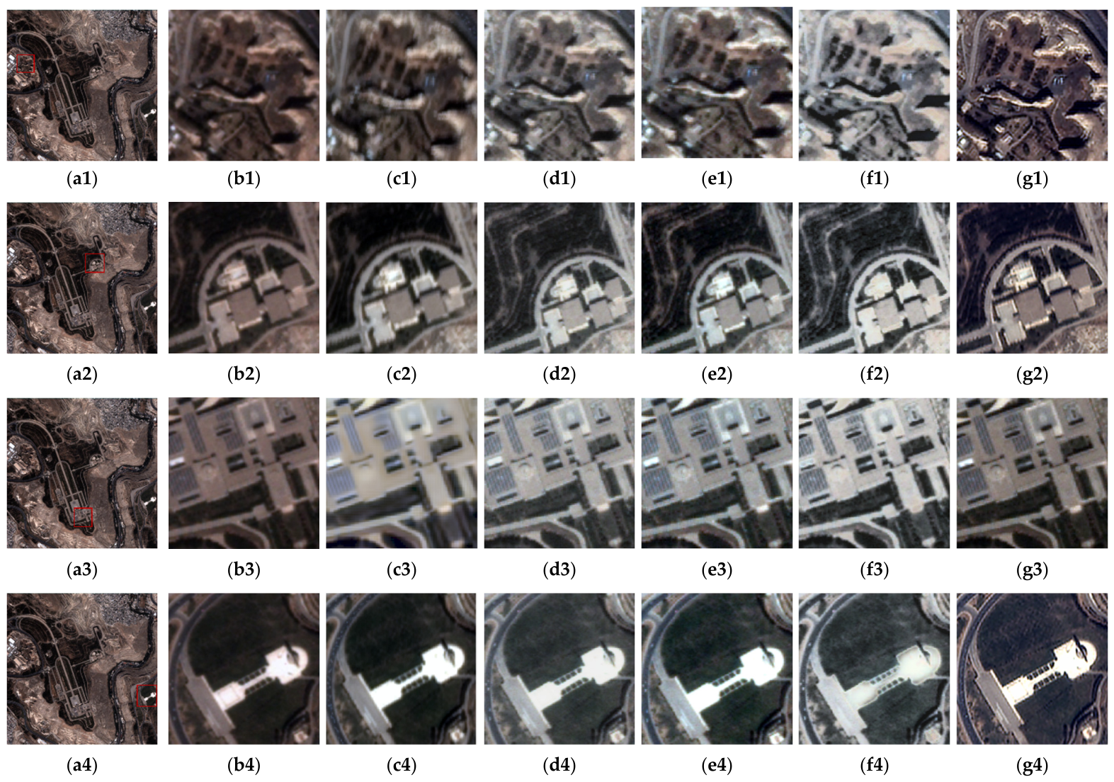
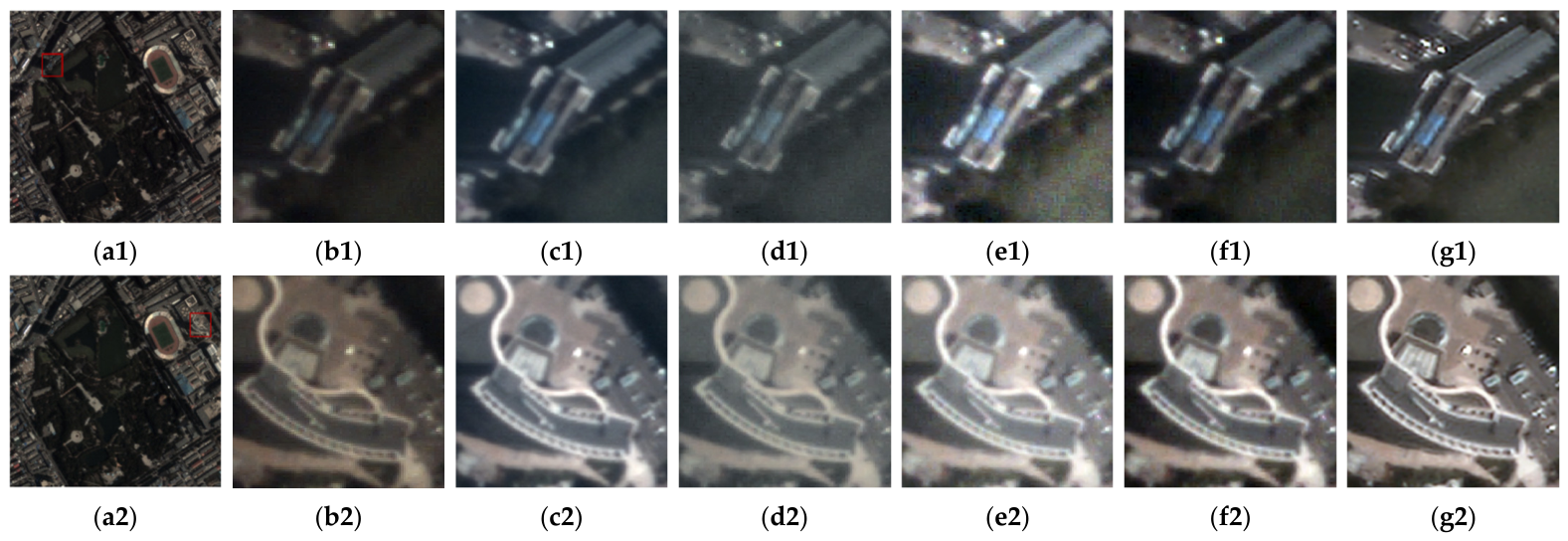
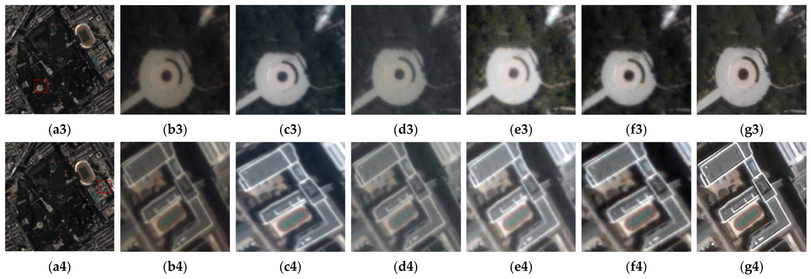
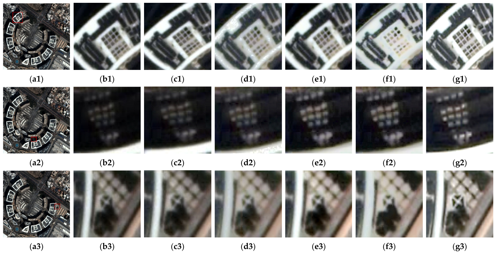
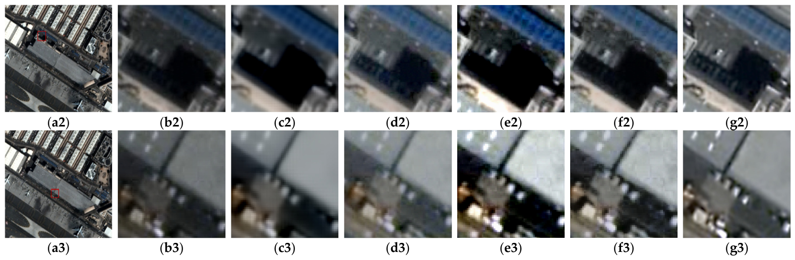
Figure 3, Figure 4, Figure 5 and Figure 6 compare MSR-CQI with four representative enhancement and restoration methods, SSIF [28], LLM [29], MPESPDF [30], and ALSP+ [31], on the OVS-1A, Jilin-1, and Luojia03-01 sequences. The displayed PSNR and SSIM values quantify agreement with the reserved-frame proxy under the adopted protocol; they do not establish recovery of independent information beyond the sensor native resolution. The corresponding visual comparisons are interpreted as evidence of radiometric and structural behavior on the registered grid. The PSNR and SSIM values calculated against the proxy reference are summarized in

Table 1. PSNR and SSIM against the proxy reference for four real satellite video sequences after registration to a common LR grid.

Dataset	Bicubic PSNR/SSIM	MSR-CQI PSNR/SSIM	ΔPSNR/ΔSSIM
Jilin-1	45.7883/0.9855	49.6786/0.9961	+3.8904/+0.0106
OVS-1A	29.9918/0.8492	30.5610/0.8844	+0.5693/+0.0352
Luojia ROI-1	31.7647/0.9384	32.4881/0.9593	+0.7234/+0.0209
Luojia ROI-2	35.4393/0.9461	37.7037/0.9704	+2.2644/+0.0243

Note: PSNR and SSIM are calculated against the LR-derived proxy reference. The effective PSF was Identity 1 × 1 for all four sequences.

.

Representative regions in Figure 3, Figure 4, Figure 5 and Figure 6 show differences around building edges, road boundaries, narrow linear structures, and locally high-contrast targets. These real-data results are interpreted as radiometric and structural behavior on the registered grid. Because the reference is constructed from reserved LR observations, neither the visual comparisons nor the proxy PSNR/SSIM values demonstrate recovery of independent spatial information beyond the native sensor sampling.

Across the four real sequences, visible differences occur mainly along building edges, narrow linear structures, and locally high-contrast targets. These real-data results are interpreted as multiframe restoration and qualitative evidence of structural and radiometric behavior on the common grid. Quantitative evidence for spatial super-resolution is evaluated separately using controlled experiments with known HR references in Section 3.2 and Section 3.4.

3.2. Controlled ×2 Reconstruction with Known HR

The controlled ×2 experiment provides the principal assessment of spatial reconstruction using a known HR reference. A 1024 × 1024 region from Jilin-1 frame 0147 was used as the HR reference. Eight 512 × 512 LR observations were generated using prescribed subpixel shifts, a normalized 7 × 7 Gaussian PSF ($\sigma =1.2$), exact 2 × 2 block averaging, and additive Gaussian noise with a standard deviation of 1/255. Metrics were calculated after excluding 16 HR pixels from each image border.

The reconstruction parameters for MSR-CQI were determined using a spatially separate validation region and were then kept unchanged for evaluation on the HR test region. Bicubic interpolation, IBP [6], TV [24], and OGS-TV [23] were evaluated under the same degradation and evaluation conditions. The resulting PSNR and SSIM values are listed in

Table 2. Controlled ×2 reconstruction using a known HR reference.

Method	PSNR (dB)	SSIM
Bicubic	38.473980	0.955010
IBP	42.770477	0.972880
TV	41.933434	0.972247
OGS-TV	42.845072	0.975325
MSR-CQI (complete formulation)	42.837530	0.975250
MSR-CQI	42.871415	0.975576

.

MSR-CQI achieved 42.8714 dB and 0.9756, compared with 42.8451 dB and 0.9753 for OGS-TV, 42.7705 dB and 0.9729 for IBP, 41.9334 dB and 0.9722 for TV, and 38.4740 dB and 0.9550 for bicubic interpolation. The difference between MSR-CQI and OGS-TV was 0.0263 dB in PSNR and 0.00025 in SSIM, indicating comparable reconstruction accuracy under this controlled setting.

3.3. Brightness-Order and Information-Fidelity Evaluation

To complement the controlled spatial-reconstruction experiment in Section 3.2, LOE and VIF were evaluated for the real sequence radiometric/restoration comparison using MPESPDF, LLM, ALSP+, SSIF, and MSR-CQI. Lower LOE indicates better preservation of relative brightness ordering, whereas higher VIF indicates greater reference-related information fidelity. Using the same image pairs for all methods, MSR-CQI obtained the lowest LOE and the highest VIF among the five evaluated methods for all four sequences. The complete LOE and VIF results for the four real sequences are given in

Table 3. Recomputed brightness-order and information-fidelity metrics for the real sequence radiometric/restoration comparison.

Dataset	Method	LOE ↓	VIF ↑
Jilin-1	SSIF	893.8971	0.5582
	LLM	369.0933	0.7034
	MPESPDF	923.186	0.6776
	ALSP+	436.0116	0.5396
	MSR-CQI	203.542	0.991
OVS-1A	SSIF	560.5136	0.7238
	LLM	384.0939	0.898
	MPESPDF	344.4099	0.8062
	ALSP+	671.8348	0.6837
	MSR-CQI	163.211	0.9682
Luojia ROI-1	SSIF	795.5671	0.6015
	LLM	248.7376	0.9301
	MPESPDF	417.7268	0.6535
	ALSP+	276.953	0.5142
	MSR-CQI	100.75	0.9818
Luojia ROI-2	SSIF	372.7186	0.585
	LLM	337.5856	0.9688
	MPESPDF	474.1136	0.7683
	ALSP+	725.0659	0.6422
	MSR-CQI	272.035	0.9822

Note: ↓ indicates that lower values are better; ↑ indicates that higher values are better. Bold values indicate the best result for each dataset. LOE is interpreted as a brightness-order diagnostic, whereas VIF measures reference-related information fidelity.

. Specifically, its LOE/VIF values were 203.5421/0.9910 for Jilin-1, 163.2105/0.9682 for OVS-1A, 100.7500/0.9818 for Luojia03-01 ROI-1, and 272.0345/0.9822 for Luojia03-01 ROI-2.

3.4. Spatial Super-Resolution Comparison Under Identical Input Conditions

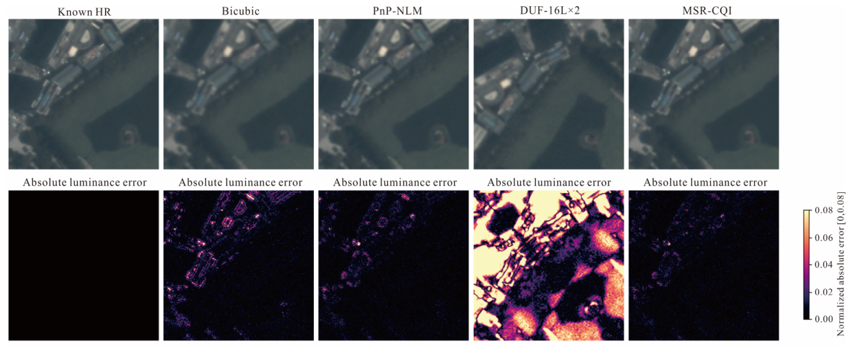
A spatially separate 256 × 256 Jilin-1 region from frame 0147 was used as the HR reference for an additional ×2 comparison using seven input frames. Each method received the same seven 128 × 128 LR observations and was evaluated on the same border-excluded HR region.

PnP-NLM combines the plug-and-play reconstruction framework [32] with a nonlocal-means denoiser [33]. Its reconstruction parameters were determined using a spatially separate validation region. DUF-16L [34] was evaluated using the published ×2 weights without additional training on the present satellite video data. The results of the seven-frame comparison are summarized in

Table 4. Controlled ×2 comparison using the same seven LR input frames and evaluation region.

Method	PSNR (dB)	SSIM
MSR-CQI	43.1049	0.971385
PnP-NLM	42.1369	0.969819
Bicubic	39.5793	0.955296
DUF-16L ×2	38.1675	0.940420

.

MSR-CQI achieved 43.1049 dB PSNR and 0.971385 SSIM. PnP-NLM achieved 42.1369 dB and 0.969819, bicubic interpolation achieved 39.5793 dB and 0.955296, and DUF-16L achieved 38.1675 dB and 0.940420.

These values describe the performance of the tested implementations under the adopted seven input frames ×2 setting. They are not intended as a general ranking among different reconstruction frameworks.

3.4.1. Effect of Retaining the Original Sampling Shifts

The paired experiment compares two representations of the same measured sampling shifts. In the original-grid reconstruction, the translations remain explicit in the forward and adjoint operators. In the common-grid reconstruction, each LR observation is bilinearly resampled onto the reference grid, and the residual transformation is set to the identity. All other reconstruction settings are unchanged. The paired results are summarized in

Table 5. Comparison between reconstruction on the original sampling grid and reconstruction after registration to a common grid.

Evaluation Setting	Reconstruction	PSNR (dB)	SSIM
Controlled, known HR	Original sampling grid	45.7461	0.98046
	Common grid after registration	45.0380	0.97904
Jilin-1, LR proxy	Original sampling grid	45.4288	0.98921
	Common grid after registration	46.4211	0.99186
	Bicubic reference frame	44.1409	0.98252

Note: All paired reconstructions used the same data, PSF, regularization parameters, ×2 scale, and 30 ADMM iterations.

.

For the controlled experiment with a known HR reference, reconstruction on the original sampling grid achieved 45.7461 dB PSNR and 0.98046 SSIM, whereas reconstruction after registration to a common grid achieved 45.0380 dB and 0.97904. Retaining the measured shifts in the observation operators therefore increased PSNR by 0.7081 dB and SSIM by 0.00143 for the tested shift pattern.

The eight measured translations occupied all four coarse phase regions defined in Section 2.6. Their distribution was nevertheless nonuniform, with a minimum pairwise toroidal separation of 0.0876 LR pixel. The result therefore reflects retention of the measured phase distribution and should not be interpreted as evidence of ideal 2 × 2 lattice sampling.

For the real Jilin-1 ROI, the common-grid reconstruction produced higher proxy PSNR and SSIM than reconstruction on the original sampling grid. The opposite ranking relative to the controlled experiment with a known HR reference shows that agreement with the LR-derived proxy is not equivalent to agreement with independent HR. The real-data proxy values are therefore used only as relative consistency measures.

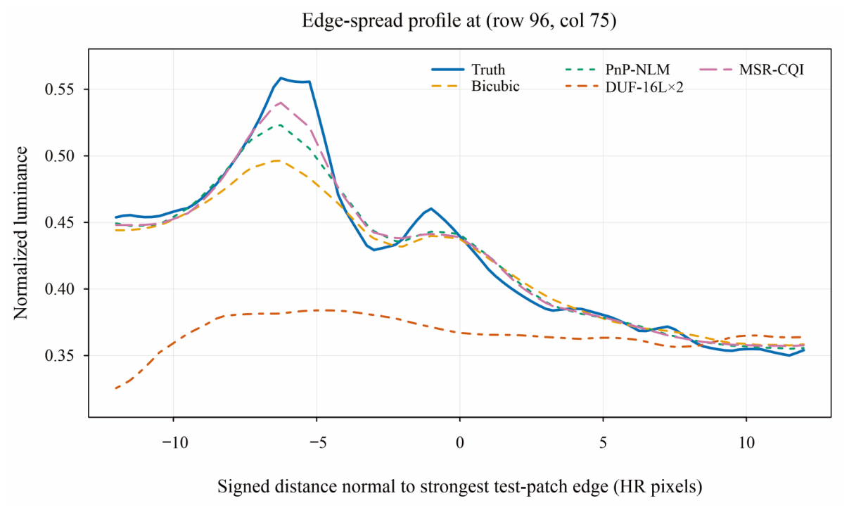
Figure 7 compares the reconstructed images and absolute luminance-error maps under the identical seven input frames ×2 setting. Figure 8 further shows the edge-normal luminance profiles at a representative high-gradient location selected from the known HR reference. These visual diagnostics are used to complement the PSNR and SSIM results rather than to provide independent quantitative metrics.

3.4.2. Spatially and Temporally Disjoint PSF Validation Across Real Sequences

The spatially separated PSF evaluation selected Identity 1 × 1 in both region directions for all four real satellite video sequences. The same kernel also produced the highest proxy PSNR/SSIM on each corresponding nonoverlapping evaluation region.

For Jilin-1, the two evaluation-region results were 46.0732 dB/0.990160 and 40.6440 dB/0.983212. For OVS-1A, the corresponding values were 27.3806 dB/0.780305 and 34.1743 dB/0.951834. Luojia03-01 ROI-1 produced 36.2312 dB/0.970163 and 34.0007 dB/0.968219, whereas ROI-2 produced 37.5471 dB/0.974994 and 38.4330 dB/0.978255.

For OVS-1A and the two Luojia03-01 ROIs, the additional central RGB region gave the same PSF result. Identity 1 × 1 produced 29.7089 dB/0.875233 for OVS-1A, 32.7124 dB/0.963236 for ROI-1, and 38.3502 dB/0.973120 for ROI-2.

These results show that the Identity PSF remained consistent across the tested spatial regions. Because the evaluation references are derived from reserved LR observations, the reported values assess regional consistency of the PSF determination and proxy agreement rather than absolute spatial-resolution recovery.

3.5. Analysis of Individual Reconstruction Terms and Parameter Sensitivity

The contribution of the principal reconstruction terms was examined by removing individual components in turn. A complete $2^5$ factorial experiment was performed for OVS-1A. For Jilin-1, the RGB component comparison used the Identity 1 × 1 PSF determined by the spatially separated evaluation. The two Luojia03-01 ROIs were evaluated using the complete formulation, four with individual components removed configurations, and a fixed Gaussian-PSF comparison under unchanged for each sequence reconstruction settings.

The second-order term $\beta \parallel {\nabla }^{2}z{\parallel }_p^p$ is referred to hereafter as the high-order nonconvex total-variation (HONCTV) regularizer.

Table 6. Component comparison based on the proxy reference.

Variant	Jilin-1	OVS-1A	Luojia ROI-1	Luojia ROI-2
Complete	49.6786/0.9961	30.5610/0.8844	32.4881/0.9593	37.7037/0.9704
Uniform weights	49.7431/0.9960	30.9731/0.8957	32.4769/0.9600	37.9041/0.9719
No intensity prior	49.6793/0.9961	30.5610/0.8844	32.4880/0.9593	37.7037/0.9704
No OGS	49.3917/0.9954	30.4024/0.8745	32.3920/0.9567	37.4114/0.9678
No HONCTV	49.6816/0.9961	30.5603/0.8844	32.4870/0.9593	37.6967/0.9704
Gaussian PSF	48.1507/0.9945	29.9437/0.8659	31.2467/0.9486	36.1182/0.9621

Note: Each entry is PSNR (dB)/SSIM. “Gaussian PSF” denotes a 7 × 7 Gaussian kernel with $\sigma =1.2$.

summarizes the component-comparison results for the real sequences. Replacing the static observation weights with uniform weights increased proxy PSNR by 0.0644 dB for Jilin-1, 0.4121 dB for OVS-1A, and 0.2004 dB for Luojia ROI-2. Luojia ROI-1 showed a negligible PSNR change, and the SSIM differences were small and mixed. Static observation weighting therefore did not provide a consistent improvement across the four sequences.

Removing OGS reduced both PSNR and SSIM for all four sequences. For Jilin-1, the reduction was 0.2869 dB in PSNR and 0.000635 in SSIM. Replacing Identity 1 × 1 with the fixed 7 × 7 Gaussian PSF reduced Jilin-1 proxy PSNR by 1.5279 dB and SSIM by 0.001584. Across the four sequences, the fixed Gaussian PSF reduced proxy PSNR by approximately 0.62–1.59 dB.

Removing the weak intensity prior or HONCTV produced smaller and, in some cases, sign-reversed metric changes. Under the present protocol against the proxy reference, OGS and effective-PSF specification therefore showed the most consistent numerical influence among the tested model components.

The sequential OGS → HONCTV procedure and the joint ADMM formulation produced similar PSNR and SSIM values. The sequential procedure yielded slightly higher values in two evaluated cases, whereas the joint formulation incorporates OGS and high-order regularization within a single inverse problem. The principal distinction between the two procedures is therefore the organization of the reconstruction terms rather than a uniform numerical advantage.

For OVS-1A, the factorial analysis showed an average PSNR effect of +1.0530 dB for effective-PSF specification and +0.5468 dB for OGS. Static observation weighting produced a negative average effect in this sequence, whereas the intensity prior and HONCTV had comparatively small individual effects. The full factorial analysis was performed only for OVS-1A and is not generalized to the other sequences.

The numerical behavior of the ADMM solution was also recorded over the fixed 30-iteration budget. For the representative OVS-1A runs, the objective value decreased throughout the iterations and all PCG calls returned flag 0. Nonzero primal and dual residuals remained after 30 iterations; these values are reported as numerical diagnostics rather than as evidence of formal convergence.

3.6. Sensitivity to Registration Error, Noise, Parallax, Motion, and Structural Change

Controlled sensitivity experiments were performed on a separate 128 × 128 HR region using three fixed realizations for each perturbation level. The experiments examined residual registration error, Gaussian noise, localized parallax, persistent target motion, and structural change. The resulting values are specific to the adopted synthetic conditions and are used to describe sensitivity rather than general operating limits.

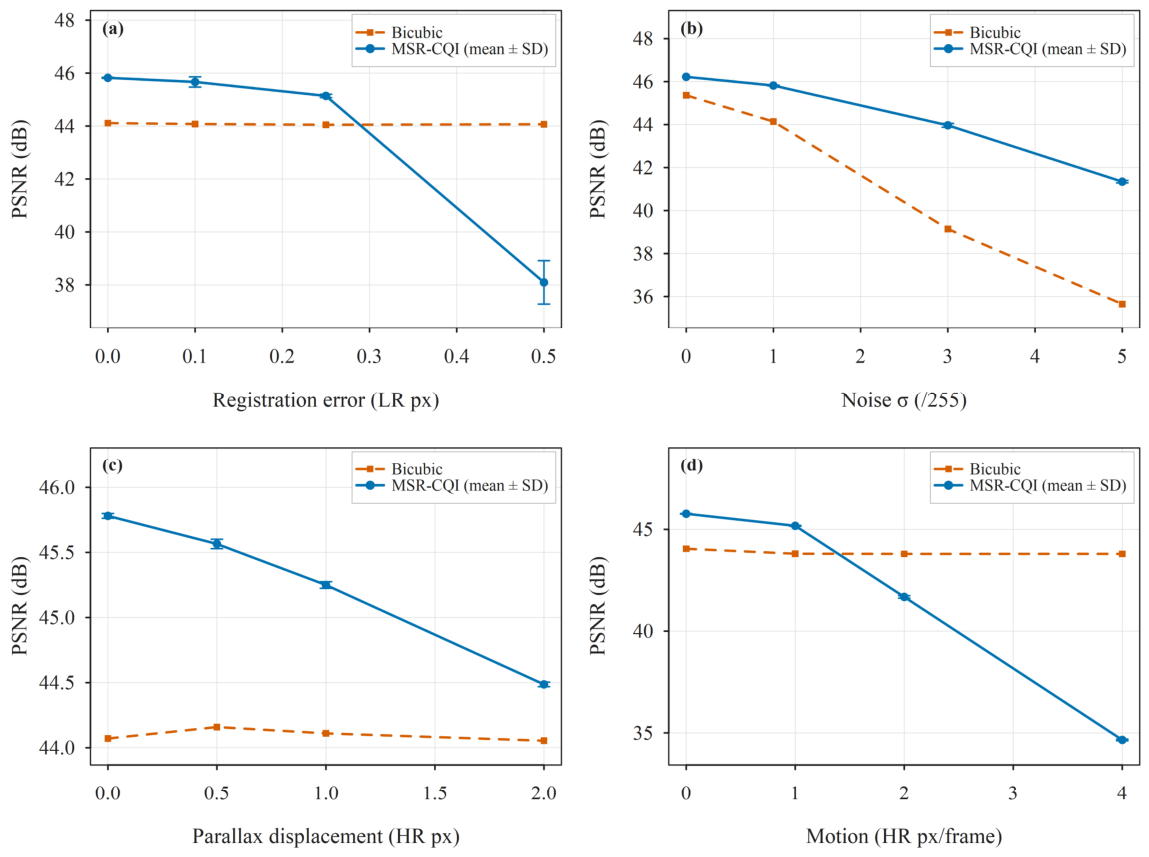
At a residual registration error of 0.5 LR pixel, MSR-CQI achieved 38.0945 ± 0.8214 dB, compared with 44.0678 dB for center-frame bicubic interpolation. At a Gaussian-noise level of $\sigma =5/255$, MSR-CQI achieved 41.3437 ± 0.0567 dB, exceeding bicubic interpolation by 5.6975 dB. Representative endpoint values for registration error, noise, parallax, and target motion are summarized in

Table 7. Sensitivity results for selected perturbation levels.

Perturbation Level	MSR-CQI PSNR (dB) Mean ± SD	Bicubic PSNR (dB)	ΔPSNR (dB)
Registration error, 0.5 LR px	38.0945 ± 0.8214	44.0678	−5.9733
Noise, $\sigma =5/255$	41.3437 ± 0.0567	35.6462	+5.6975
Localized parallax, 2 HR px	44.4864 ± 0.0175	44.0538	+0.4326
Target motion, 2 HR px/frame	41.6819 ± 0.0615	43.7967	−2.1148
Target motion, 4 HR px/frame	34.6540 ± 0.0394	43.7976	−9.1437

, while the persistent structural-change results are reported in

Table 8. Sensitivity to persistent structural change.

Changed Area	MSR-CQI PSNR (dB)	MSR-CQI SSIM	Bicubic PSNR (dB)	RMSE in Changed Region
0%	45.8155 ± 0.0267	0.987432 ± 0.000067	44.0960 ± 0.0686	0.00512/0.00624
1%	30.3959 ± 1.0277	0.972248 ± 0.000943	44.0609 ± 0.0270	0.23971/0.00576
5%	23.1899 ± 0.9473	0.941655 ± 0.011447	44.1156 ± 0.0725	0.25140/0.00566
10%	20.1021 ± 0.9079	0.912444 ± 0.024903	44.0943 ± 0.0624	0.25478/0.00565

Note: Values are reported as mean ± SD. The last column gives MSR-CQI/Bicubic RMSE within the changed region.

.

For localized parallax of 2 HR pixels, MSR-CQI retained a small positive difference of 0.4326 dB relative to bicubic interpolation. Persistent target motion had a stronger effect. At 2 HR pixels per frame, MSR-CQI was 2.1148 dB below bicubic interpolation, and at 4 HR pixels per frame the difference increased to −9.1437 dB.

Persistent structural change produced a similar loss of multiframe consistency. With no injected change, MSR-CQI exceeded bicubic interpolation by approximately 1.72 dB. When persistent change affected 1% of the HR image, MSR-CQI fell below the center-frame bicubic result, and the discrepancy increased as the changed area expanded to 5% and 10%. The PSNR trends for registration error, Gaussian noise, localized parallax, and persistent target motion are shown in Figure 9.

3.7. Computational Efficiency, Memory, and Runtime Analysis

The computational cost is dominated by the PCG solution of the z-subproblem, with a leading per-iteration complexity of $O\left(K_{\mathrm{p}\mathrm{c}\mathrm{g}}NM\right)$, in addition to the OGS update. Across three full-RGB OVS-1A runs, peak working memory is 2.820 ± 0.001 GiB, or 1.706 GiB above the recorded baseline. In a matched reduced-iteration test performed in MATLAB R2025b (The MathWorks, Inc., Natick, MA, USA), the CPU and NVIDIA GeForce GTX 1050 Ti Max-Q GPU (NVIDIA Corporation, Santa Clara, CA, USA) require 3.69 ± 0.79 s and 4.42 ± 1.63 s, respectively. No runtime reduction was observed with the tested GPU implementation on the reported hardware configuration.

4. Discussion

The results distinguish two different roles of multiframe information in the present study. In the controlled experiments with known HR references, retaining measured or prescribed sampling shifts within the forward model improved reconstruction relative to LR pre-registration under the tested shift pattern. This result is consistent with the classical MFSR principle that complementary sampling locations should be represented explicitly when spatial-detail recovery is the objective.

The real satellite video experiments address a different problem. Because the principal real-data pathway first resamples the observations onto a common LR grid, these experiments evaluate multiframe restoration after resampling to a common LR grid rather than direct acquisition-phase super-resolution. The LR-derived proxy reference provides a consistent basis for comparison within each sequence but contains no independent spatial information beyond the original sampling. The opposite rankings obtained for the two reconstruction approaches against known HR and against the real-data proxy further show that proxy agreement is not equivalent to HR reconstruction accuracy. Proxy PSNR and SSIM should therefore be interpreted only as relative consistency measures.

The controlled ×2 experiments also show that the proposed formulation provides reconstruction accuracy comparable to OGS-TV under the adopted degradation conditions. In the separate seven-frame comparison, MSR-CQI produced higher PSNR and SSIM than the tested PnP-NLM and DUF-16L implementations. These results are specific to the adopted inputs, parameter settings, and available implementations and should not be interpreted as a general ranking among reconstruction approaches.

The component comparisons clarify which terms contribute most consistently under the protocol used for the real sequences. OGS and effective-PSF specification produced the largest and most consistent changes in proxy PSNR and SSIM. By comparison, the weak intensity prior, HONCTV, and static observation weighting produced smaller or scene-dependent effects. In particular, uniform observation weights improved proxy PSNR for Jilin-1, OVS-1A, and Luojia ROI-2. Static observation weighting should therefore be regarded as an optional component rather than a necessary source of reconstruction improvement.

The intensity weighting centered at 0.5 is an empirical intensity-range term defined in the normalized digital domain. It is not derived from sensor exposure time, gain, full-well capacity, radiometric calibration, saturation thresholds, or a calibrated noise model. A more physically grounded weighting strategy would require sensor-dependent noise and saturation characteristics, registration uncertainty, local structural consistency, occlusion information, and possibly reconstruction residuals.

The spatially separated PSF evaluation reduced the risk that the effective PSF was determined and assessed on the same image region. Identity 1 × 1 remained consistent across both nonoverlapping region directions for all four real sequences and across the additional central regions available for OVS-1A and the Luojia03-01 ROIs. These results support the regional consistency of the selected effective reconstruction kernel. They do not identify the physical sensor PSF or MTF and do not establish absolute resolution improvement.

The controlled sensitivity experiments further define the applicability of the current formulation. Residual registration error, persistent target motion, and structural change can introduce spatially inconsistent observations that violate the common-scene assumption underlying multiframe reconstruction. The method is therefore most appropriate for short satellite video sequences with limited geometric and structural variation. Explicit treatment of motion, occlusion, and local parallax would be required for more dynamic scenes.

Several limitations remain. First, the principal real-data evaluation uses common-grid resampling, and the real-data experiment performed on the original sampling grid is limited to a single Jilin-1 Band01 region. Extension to full RGB sequences and additional sensors is required. Second, none of the real satellite video sequences provides an independent HR, sensor MTF, edge-response, or resolution-target reference. Third, the current static observation weighting does not provide consistent improvement across scenes and is not based on a physical sensor-noise model. Fourth, the factorial component analysis was performed only for OVS-1A, and the available matched video-SR comparisons remain limited.

Future work should therefore extend reconstruction on the original sampling grid to additional sensors and full-resolution RGB sequences, incorporate independent sensor-resolution evidence where available, and improve handling of motion, occlusion, and parallax. Observation weighting should also be reformulated using sensor-specific noise and saturation characteristics, registration uncertainty, and local structural consistency. More efficient implementations are additionally required for large satellite video sequences.

5. Conclusions

This study presents MSR-CQI as a model-based radiometric and spatial reconstruction framework for short optical satellite video sequences. The formulation combines multiframe fidelity, effective blur representation, a weak intensity prior, overlapping-group sparsity, high-order regularization, intensity bounds projection, and optional static observation weighting within an ADMM framework.

Controlled experiments with known HR references show that retaining measured sampling shifts explicitly in the forward model improves reconstruction relative to LR pre-registration under the tested shift pattern. Under identical ×2 inputs, the proposed formulation also provided reconstruction accuracy comparable to the strongest model-based baseline evaluated in the controlled experiment and higher PSNR and SSIM than the tested PnP-NLM and DUF-16L implementations.

For the real satellite video sequences, the principal real-data results are interpreted as multiframe radiometric and spatial restoration after registration and resampling to a common LR grid rather than as direct sampling-phase super-resolution. The reserved-frame references are derived from LR observations and therefore provide relative consistency measures only; they cannot establish recovery beyond native sensor sampling. Spatially separated PSF evaluation eliminated direct reuse of the PSF-determination region, while the component comparisons showed that OGS and effective-PSF specification had more consistent effects than the weak intensity term, HONCTV, or static observation weighting.

The present method is most applicable to short sequences with limited geometric and structural change. Future work should extend reconstruction on the original sampling grid to full RGB data and additional sensors, incorporate independent sensor-resolution validation, explicitly address motion and occlusion, and improve computational efficiency.