Article

STAMP-GAN: A Spatiotemporal Attention-Modulated Generative Adversarial Network for Precipitation Nowcasting


1
School of Artificial Intelligence, Zhejiang A&F University, Hangzhou 311300, China
2
School of Artificial Intelligence, Guangdong Polytechnic Normal University, Guangzhou 510665, China
3
School of Electronic and Information Engineering, Nanjing University of Information Science and Technology, Nanjing 210044, China
4
Hangzhou Meteorological Observatory, Hangzhou 310051, China
*
Author to whom correspondence should be addressed.
Remote Sens. 2026, 18(17), 3026; https://doi.org/10.3390/rs18173026
Submission received: 30 May 2026 / Revised: 6 August 2026 / Accepted: 1 September 2026 / Published: 4 September 2026

Highlights

  • STAMP-GAN improves regional hourly precipitation sequence prediction.
  • Attention-modulated ConvLSTM captures multiscale spatiotemporal evolution.
  • Dual-branch temporal discrimination strengthens long-lead forecast structure.
  • Hybrid intensity-aware losses improve heavy-precipitation representation.

Abstract

Precipitation nowcasting aims to predict short-term precipitation evolution over forecast lead times of 1–6 h and can support hydrological-risk and disaster-prevention applications when near-real-time observations are available. However, precipitation forecasting remains challenging because of rapid spatiotemporal evolution, spatial displacement, and the difficulty of representing localized high-intensity precipitation. To address these issues, this study proposes STAMP-GAN, a spatiotemporal attention-modulated generative adversarial network for regional precipitation sequence prediction. STAMP-GAN combines an AM-ConvLSTM temporal evolution module with spatial attention, efficient channel attention, large-receptive-field context modeling, and temporal-index-conditioned feature modulation. A spatially aligned two-dimensional digital elevation model (DEM) field is retained as static auxiliary geographical information. The STAMP-Net generator uses hierarchical multi-scale feature extraction to reconstruct precipitation structures at different spatial scales while a dual-branch temporal PatchGAN provides adversarial supervision for both the complete forecast sequence and the final three forecast frames. A hybrid objective combines regression, event-based, structural, temporal, and adversarial constraints. Experiments on the ERA5 and CMA-S datasets show that, compared with the best-performing baseline for each metric, STAMP-GAN achieves relative CSI improvements of approximately 6.5% and 9.5%, respectively. The proposed framework provides a data-driven approach for retrospective hourly regional precipitation sequence prediction under gridded meteorological-data conditions, rather than a fully validated operational real-time nowcasting system.

1. Introduction

Precipitation nowcasting generally refers to quantitative short-term precipitation forecasting within a 0–6 h lead-time window [1]. When driven by near-real-time observation streams with sufficiently low latency, such forecasts can support disaster prevention and mitigation, urban flood-risk management, traffic safety, and emergency response. Unlike synoptic-scale forecasting, precipitation nowcasting focuses on rapidly evolving convective systems characterized by pronounced spatial heterogeneity and high temporal variability, making accurate prediction highly challenging [2].
In recent decades, the combined effects of global climate change and rapid urbanization have contributed to marked increases in both the frequency and intensity of extreme short-duration heavy precipitation events. The catastrophic “7·20” rainstorm [3] in Zhengzhou in 2021 caused severe urban waterlogging and substantial casualties, highlighting the need for timely and reliable short-term precipitation information. To evaluate the proposed method under representative real-world conditions, Zhejiang Province in eastern China was selected as the experimental region. The region is characterized by complex mountainous terrain in the west and highly urbanized coastal plains in the east, and it frequently experiences Meiyu-season rainfall and typhoon-related convective systems. Together, these factors give rise to precipitation patterns with strong spatial variability and pronounced extremes [4]. Therefore, developing nowcasting models capable of representing spatially heterogeneous and high-impact precipitation processes over complex terrain has broad scientific significance and operational value.
Regional precipitation nowcasting is also an important downstream application of Earth observation and remote sensing. Modern regional forecasting systems increasingly integrate gridded meteorological observation products, reanalysis datasets, station-derived fields, and terrain information to improve the representation of rapidly evolving precipitation systems. Developing deep-learning methods capable of effectively exploiting these multi-source geospatial observation products therefore remains an important research topic in remote sensing applications. Optical-flow [5] methods infer the spatiotemporal evolution of precipitation fields and are computationally efficient. However, these methods assume the spatial stationarity of precipitation structures. Consequently, their performance deteriorates rapidly beyond lead times of 30–60 min, particularly when capturing convective initiation and dissipation. Early nowcasting systems mainly relied on optical-flow concepts and used Lagrangian extrapolation methods based on radar echo fields, such as STEPS [6] and PySTEPS [7]. In addition, radar-echo extrapolation methods [2,8] do not adequately account for the dynamic evolution of precipitation systems, limiting their applicability at longer forecast lead times. In this study, gridded reanalysis products and station-interpolated observation datasets were adopted as multi-source geospatial observation products to investigate the capability of deep generative models under different meteorological observation conditions and to improve regional applicability in areas with limited radar coverage. Compared with optical-flow methods, numerical weather prediction (NWP) [9] models provide more physically consistent dynamical forecasts. However, they are computationally expensive, and their spatial and temporal resolutions are often insufficient for real-time, high-precision precipitation nowcasting.
The rapid development of deep learning has substantially advanced precipitation nowcasting [10,11]. Convolutional recurrent architectures, such as ConvLSTM [12] and TrajGRU [13], established the feasibility of end-to-end spatiotemporal learning from precipitation sequences, while encoder–decoder networks, such as U-Net++ [14], improved the recovery of spatial details. Physics-informed methods, such as PhyDNet [15], and attention-based architectures, such as Swin Transformer [16], further enhanced feature representation and spatiotemporal structural regularization. More recently, GAN-based methods, represented by DGMR [17], SpateGAN [18], and related ERA5-based generative downscaling approaches [19], and diffusion-based methods, represented by PreDiff [20] and Diffusion Nowcasting [21], have shown strong potential for generating sharp and probabilistic precipitation fields. Large-scale data-driven models, such as GraphCast [22] and MetNet-3 [23], have achieved substantial advances in medium-range forecasting; however, their direct transfer to kilometer-scale and hourly regional nowcasting remains challenging because of scale mismatch and regional-data constraints.
Despite these advances, existing precipitation sequence prediction methods still face several limitations. First, multi-step prediction errors accumulate with increasing forecast lead times, resulting in blurred precipitation structures, spatial displacement errors, and intensity attenuation in later forecast frames. Second, many generative precipitation forecasting methods apply relatively uniform constraints across different prediction times, which limits their ability to provide enhanced supervision for later frames where structural degradation becomes more pronounced. Third, pixel-wise regression losses tend to produce over-smoothed precipitation fields and insufficiently penalize misplaced or underestimated localized heavy-precipitation cores. Furthermore, precipitation systems exhibit complex spatial structures across multiple scales, ranging from large-scale precipitation bands to localized convective cells, making it difficult for single-scale architectures to simultaneously preserve broad precipitation organization and fine-scale extreme rainfall features. Therefore, a generative forecasting framework that jointly enhances temporal evolution modeling, multi-scale spatial reconstruction, long-lead structural constraints, and intensity-sensitive optimization is required.
To address these limitations, this study proposes STAMP-GAN, a Spatiotemporal Attention-Modulated Precipitation Generative Adversarial Network, as a novel generative nowcasting framework. The proposed model is evaluated on two independent datasets: an ERA5 reanalysis-based gridded dataset containing multiple meteorological variables and a high-resolution station-observation interpolation dataset. In both datasets, the spatially aligned two-dimensional DEM field is incorporated as a static auxiliary input channel to provide background elevation information. The DEM field remains unchanged across time steps and is used only as supplementary geographical information rather than as an explicit representation of terrain–precipitation physical processes. Each dataset is used independently for model training and evaluation to assess the generalizability of the proposed framework across different data sources. The main contributions of this study are summarized as follows: First, an AM-ConvLSTM temporal evolution module is proposed. It integrates spatial attention, efficient channel attention, and large-receptive-field context modeling into the recurrent state-update process to enhance the representation of critical precipitation regions, effective feature channels, and long-range spatial dependencies. A lightweight temporal-index-conditioned feature modulation mechanism is further introduced to provide explicit sequence-position information for the shared recurrent unit. Second, a STAMP-Net generator with a multi-scale fusion bottleneck is designed. Through parallel multi-scale feature extraction, residual feature representation, and hierarchical skip connections, the generator simultaneously reconstructs large-scale precipitation structures and localized heavy-precipitation details. Third, a dual-branch temporal PatchGAN discriminator is proposed, comprising a global discriminator that covers the full forecast sequence and a focal discriminator that concentrates on the final three frames, denoted as D last 3 . This design provides task-specific adversarial supervision for later forecast frames, where structural degradation and precipitation-intensity attenuation are generally more pronounced. Multi-seed experiments further show directionally consistent CSI improvements at moderate-to-heavy precipitation thresholds, although the effect is interpreted cautiously because statistical significance at the conventional 0.05 level is not established with five paired runs. Fourth, a hybrid loss-function framework is constructed by combining Wasserstein adversarial loss, weighted L1 regression, multi-threshold focal classification loss, precipitation-occurrence supervision, and spatiotemporal structural regularization, thereby jointly improving numerical accuracy, precipitation-event identification, spatial sharpness, and structural consistency for moderate and heavy precipitation forecasting.
In summary, this study proposes STAMP-GAN, a novel deep learning framework evaluated on two independent datasets. The proposed framework focuses on improving long-lead precipitation structure preservation, multi-scale spatial representation, and intensity-sensitive forecasting using multi-source geospatial observation products, thereby providing a deep-learning framework for regional precipitation sequence prediction using multi-source geospatial observation products. The two-dimensional DEM field is retained as a static auxiliary input and is not considered an independent physical modeling component. The remainder of this paper is organized as follows: author:We corrected the “organization of the paper” summary in the Introduction so that it correctly matches the actual sections (Materials and Methods/Results/Discussion/Conclusions/Implementation and Robustness Analyses) Section 2 introduces the study area, datasets, and the proposed STAMP-GAN method; Section 3 presents the experimental results; Section 4 discusses the main findings; and Section 5 concludes the paper. Section 6 provides additional implementation details and robustness analyses.

2. Materials and Methods

2.1. Study Area

This study focuses on Zhejiang Province, China (118–122°E, 27–31°N), as shown in Figure 1. The region is characterized by a typical subtropical monsoon climate and is jointly influenced by the East Asian monsoon, Meiyu frontal systems, and typhoon activity, resulting in frequent precipitation events with pronounced spatiotemporal heterogeneity [24]. The long-term mean annual precipitation in the region ranges from approximately 1100 to 2200 mm, with rainfall mainly concentrated during the Meiyu season (May–June) and the typhoon-affected summer period. Spatially, precipitation generally decreases from the southwestern mountainous areas and southeastern coastal regions toward the northeastern plains. The terrain ranges from coastal lowlands to inland mountains with elevations exceeding 1800 m. The interaction between complex terrain and various weather systems gives rise to multi-scale precipitation structures and highly nonlinear evolution, providing a representative and challenging experimental environment for precipitation nowcasting research.

2.2. Datasets

To evaluate the applicability of the proposed framework under different data sources and spatial resolutions, two independent precipitation-nowcasting datasets were constructed, as summarized in Table 1.
The first dataset is a regular gridded dataset derived from ERA5 reanalysis, whereas the second is a higher-resolution gridded dataset generated by interpolating hourly surface-station observations, hereafter referred to as CMA-S. ERA5 uses a 16 × 16 grid with a spatial resolution of 0.25 , whereas CMA-S uses an 80 × 80 grid with a spatial resolution of 0.05 .
The two datasets were treated as separate forecasting tasks. STAMP-GAN and all comparison models were initialized, trained, validated, and tested independently on each dataset. No model weights, learned feature representations, normalization statistics, or intermediate states were transferred or shared between ERA5 and CMA-S. Therefore, the CMA-S experiment does not reuse spatial features learned from the coarser ERA5 grid, and vice versa.
The two datasets provide complementary but not directly comparable evaluation settings because they differ in data source, grid resolution, temporal coverage, precipitation distribution, and reference-field construction. Both datasets were used for retrospective model development and evaluation. ERA5 is a reanalysis product rather than a real-time observation stream, while the CMA-S field is constructed by interpolating hourly surface-station observations rather than directly using native radar or satellite image sequences. Accordingly, the experiments demonstrate retrospective hourly regional precipitation sequence prediction under gridded meteorological-data conditions and do not constitute validation of a fully operational real-time nowcasting system.
Operational deployment would require further assessment of data latency, real-time data availability, preprocessing time, inference speed, and end-to-end warning-chain reliability. Quantitative performance is therefore interpreted only through comparisons among models within the same dataset. Except for dataset-specific input and output dimensions and the adaptations required by individual baseline architectures, experiments within each dataset followed the same forecasting-task definition, chronological data-partitioning principle, preprocessing procedure, and evaluation protocol.
In both datasets, digital elevation model (DEM) information was incorporated as a static auxiliary input to account for the influence of topography on precipitation distribution and evolution. In both datasets, the spatially aligned two-dimensional digital elevation model (DEM) field was incorporated as a static auxiliary input channel to provide grid-level background elevation information. The DEM field remained unchanged across all time steps and was not used as an explicit representation of orographic precipitation processes.

2.2.1. ERA5 Reanalysis Dataset

The ERA5 dataset was constructed from the fifth-generation global atmospheric reanalysis product released by the European Centre for Medium-Range Weather Forecasts (ECMWF) [25]. Hourly single-level ERA5 data during the main rainy seasons from April to September in 2021–2024 were used. The native spatial resolution of ERA5 is 0.25 × 0.25 . After spatial cropping, the data were organized into a regular 16 × 16 grid covering the study region.
Seven meteorological variables were selected as dynamic inputs, including total precipitation (tp), 2 m dew-point temperature (d2m), 10 m zonal wind component (u10), 10 m meridional wind component (v10), mean sea-level pressure (msl), total cloud cover (tcc), and relative humidity (rh). Relative humidity was calculated from 2 m temperature (t2m) and 2 m dew-point temperature (d2m) using the saturation vapor pressure relationship. Because preliminary correlation analysis indicated a relatively weak direct correlation between t2m and precipitation, t2m was used only to derive relative humidity and was not included as an independent input variable. Total precipitation was converted to millimeters, and mean sea-level pressure was converted from Pa to hPa. All dynamic variables were temporally aligned at 1 h intervals and spatially cropped to the same 16 × 16 grid.
Data quality checks were conducted before model training. Samples containing NaN or Inf values were removed. Three extremely small negative precipitation values, ranging from approximately 3 × 10 6 to 1 × 10 7 mm, were identified in the ERA5 dataset. These values were attributable to numerical precision during data processing rather than missing observations and were therefore truncated to the physical lower bound of zero. Abnormal values in the other meteorological variables were inspected and were removed or interpolated only when they were identified as evident erroneous records. All normalization statistics, including the mean and standard deviation of continuous meteorological variables, were calculated exclusively from the training set. The same normalization parameters were then applied unchanged to the validation and test sets to avoid information leakage.
For the ERA5 dataset, the processed two-dimensional DEM field was aligned to the 0.25 grid, expanded along the temporal dimension, and concatenated with the dynamic meteorological variables as a static auxiliary input channel. Further details on DEM preprocessing and usage are provided in Section 2.2.3.

2.2.2. Station Observation Dataset (CMA-S)

To further evaluate the model under high-resolution observational constraints, a station-observation interpolated gridded dataset, denoted as CMA-S, was constructed using hourly surface precipitation observations provided by the Hangzhou Meteorological Bureau for Zhejiang Province. The original station dataset contains observations from 5243 meteorological stations within Zhejiang Province, among which regional automatic weather stations account for approximately 82%, national-level stations account for approximately 2%, and the remaining stations belong to other types. Because the station records became relatively complete from 2022 onward, observations from April to September in 2022–2024 were used.
The original station observations are irregularly distributed point measurements. To obtain regular gridded fields for convolution-based spatiotemporal prediction, inverse distance weighting (IDW) interpolation [26] was used to map the station observations onto a 0.05 × 0.05 regular grid. The IDW power parameter was set to p = 2 , and interpolation was performed independently at each hourly time step. The resulting CMA-S dataset has a spatial size of 80 × 80 , corresponding to an approximate grid spacing of 5 km over the study region.
Before interpolation, quality control was performed on the station observations. Records coded as 999999 were treated as missing values, converted to NaN, and excluded from interpolation. These records accounted for 5,373,911 observations, or 4.57% of the 117,671,073 original precipitation records. No negative values were found among the valid PRE_1h observations. Other physically unrealistic records were removed only after quality-control inspection. Missing station observations were not replaced by zero rainfall, so that artificial dry signals were not introduced into the gridded CMA-S fields. Potential extreme precipitation values were not removed solely because of their magnitude; neighboring-station consistency and temporal continuity were also considered before interpolation.
To assess how strongly the interpolated grid is constrained by the physical observation network, the great-circle distance from each grid-cell center to its nearest rain-gauge station was calculated. Of the 6400 grid cells, 5179 cells (80.92%) were located within 5 km of at least one station, while 90.88% and 94.70% were within 10 and 20 km, respectively. The mean nearest-station distance was 5.6 km. These statistics indicate that most of the CMA-S grid is supported by a relatively dense station network, although IDW interpolation can still smooth localized precipitation extremes.
For the CMA-S dataset, the processed two-dimensional DEM field was aligned to the 0.05 grid, expanded along the temporal dimension, and concatenated with the dynamic observation variables as a static auxiliary input channel. Further details on DEM preprocessing and usage are provided in Section 2.2.3.
ERA5 therefore provides a coarse-resolution reanalysis-based evaluation setting, whereas CMA-S provides a higher-resolution observation-based setting.
ERA5 and CMA-S are used as two independent gridded precipitation-sequence prediction tasks in this study. The two datasets differ in data source, grid size, spatial resolution, precipitation distribution, and reference-field construction. Therefore, their absolute verification scores are not directly compared across datasets. Instead, model performance is evaluated only among competing methods within the same dataset. For each dataset, all models are initialized, trained, validated, and tested independently, and no model weights, hidden states, learned spatial features, or normalization statistics are shared between ERA5 and CMA-S.

2.2.3. Digital Elevation Model Data

The digital elevation model used in this study was derived from the SRTMGL1 product, with an original spatial resolution of approximately 30 m [27]. The tiles covering Zhejiang Province were mosaicked, clipped to the study domain, and checked for invalid or no-data values before being resampled to match the spatial grids of the two datasets.
For ERA5, the DEM was aligned to the 0.25 regular grid, while for CMA-S it was aligned to the 0.05 grid. Bilinear interpolation was used when resizing the elevation field to an intermediate grid, followed by linear interpolation for final grid alignment. Nearest-neighbor interpolation was used only for spatial masks and was not applied to DEM elevation values.
The resulting two-dimensional DEM fields were retained as spatially explicit static auxiliary inputs and remained unchanged across the input time steps. Unlike the original design, the DEM field was not spatially averaged into a regional scalar for FiLM conditioning. The DEM therefore provides grid-level background elevation information rather than an explicit representation of orographic precipitation processes.

2.3. Data Preprocessing and Sample Construction

Each sample was constructed using a sliding temporal window of 12 consecutive hourly time steps. The first six time steps were used as the input sequence, and the subsequent six time steps were used as the prediction target, thereby defining a sequence-to-sequence forecasting task that uses the preceding 6 h of meteorological information to predict hourly precipitation at lead times of 1–6 h. This temporal configuration was predefined as a common experimental setting for all models and was not selected through optimization or comparison of alternative input-history lengths.
Given the pronounced zero inflation and heavy-tailed distribution of hourly precipitation, a dry-wet event-aware resampling strategy was applied only to the training set to increase the representation of rainy and heavy-precipitation samples during optimization. The validation and test sets retained their original chronological distributions and were not resampled. Model selection and final evaluation were therefore conducted under the natural precipitation-event frequencies of the validation and test periods.
The datasets were partitioned chronologically by year to avoid temporal information leakage. For ERA5, data from April–August 2021–2023 were used for training, September 2023 for validation, and April–September 2024 for testing. For CMA-S, data from April–August 2022–2023 were used for training, September 2023 for validation, and April–September 2024 for testing. The numbers of sliding-window samples and the precipitation-event distributions for each split are summarized in Table 15. Event statistics were calculated over all target precipitation pixels in the generated samples. Dry, light, moderate, and heavy precipitation were defined as p < 0.1 , 0.1 p < 2.5 , 2.5 p < 6 , and p 6 mm h−1, respectively.

2.4. Problem Formulation

Precipitation nowcasting aims to predict the spatial distribution and intensity evolution of precipitation over a short future horizon based on historical meteorological fields. Precipitation processes are nonlinear and spatiotemporally nonstationary, with their evolution influenced by interactions among large-scale circulation, mesoscale and small-scale dynamical processes, and local topographic conditions. In the present data-driven formulation, the DEM field is used as static auxiliary background information and does not explicitly encode these terrain-related dynamical processes. Accordingly, the forecasting task is formulated as a conditional spatiotemporal sequence prediction problem that maps historical meteorological states to future precipitation fields.
Let the current time be denoted by t and the historical input length by L. The input sequence is defined as
X = { X t L + 1 , X t L + 2 , , X t } .
Here, X τ R C × H × W denotes the multi-channel meteorological input field at time step τ , τ = t L + 1 , , t ; C is the number of input channels, and H and W denote the spatial grid dimensions. Let the forecast length be K. The ground-truth future precipitation sequence is expressed as
Y = { Y t + 1 , Y t + 2 , , Y t + K } ,
and the corresponding predicted sequence is
Y ^ = { Y ^ t + 1 , Y ^ t + 2 , , Y ^ t + K } .
where Y t + k , Y ^ t + k R H × W denote the ground-truth and predicted precipitation fields at the k-th lead time, respectively. The model therefore learns the mapping
Y ^ = F θ ( X ) ,
where F θ ( · ) denotes the proposed spatiotemporal precipitation forecasting model and θ represents its trainable parameters.
In the experiments, both L and K are set to 6. Thus, the preceding six-hourly meteorological fields are used to predict precipitation at lead times of 1–6 h. These values were predefined as part of the forecasting-task design rather than selected through a hyperparameter search or comparison of alternative history lengths. The same input-history length and forecast horizon were used for all models to ensure a consistent comparison.

2.5. Overall Architecture of STAMP-GAN

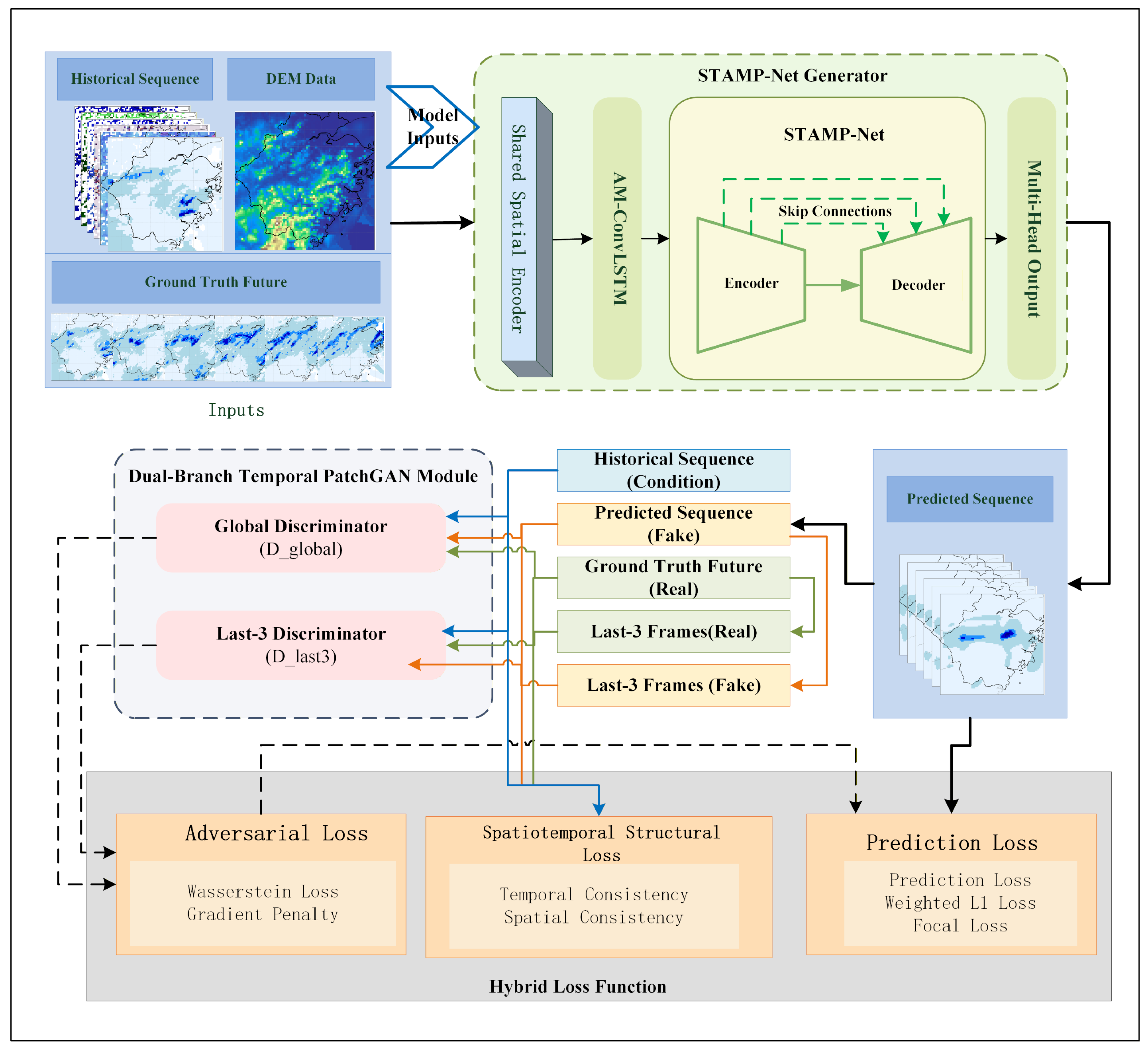
To address the spatiotemporal sequence-to-sequence prediction problem, this study proposes STAMP-GAN, a generative adversarial framework whose overall architecture is shown in Figure 2.
As shown in Figure 2, the input sequence X is first processed by a two-dimensional convolutional encoder to extract spatial features from each input frame, producing a feature sequence { F 0 , t } t = 1 L . The AM-ConvLSTM module then processes these features recurrently to model their temporal evolution and produces a compact temporal representation F temp . Temporal-position-conditioned modulation is introduced during recurrent feature evolution to provide relative sequence-position information.
The temporal representation is subsequently passed to the STAMP-Net encoder–decoder to reconstruct the future precipitation sequence Y ^ . A multi-scale fusion module is used to represent precipitation structures at different spatial scales, while hierarchical skip connections retain spatial details during reconstruction. Lead-time-conditioned modulation provides the decoder with relative forecast-position information. In addition, the spatially aligned two-dimensional DEM field is retained as static auxiliary geographical information. Unlike the original design, the DEM field is not spatially averaged into a regional scalar for FiLM conditioning.
A three-head output structure separates precipitation occurrence from precipitation-intensity estimation. During adversarial training, a dual-branch temporal PatchGAN discriminator provides supervision at two temporal ranges. The global discriminator D evaluates the complete predicted sequence, whereas the last-three-frame discriminator D last 3 focuses on the final three forecast frames, where forecast degradation is generally more pronounced. Both branches use the PatchGAN formulation to provide local structural supervision. The full framework is trained end-to-end using a hybrid loss that combines regression, event-based, structural, and adversarial constraints.

2.6. STAMP-Net Generator

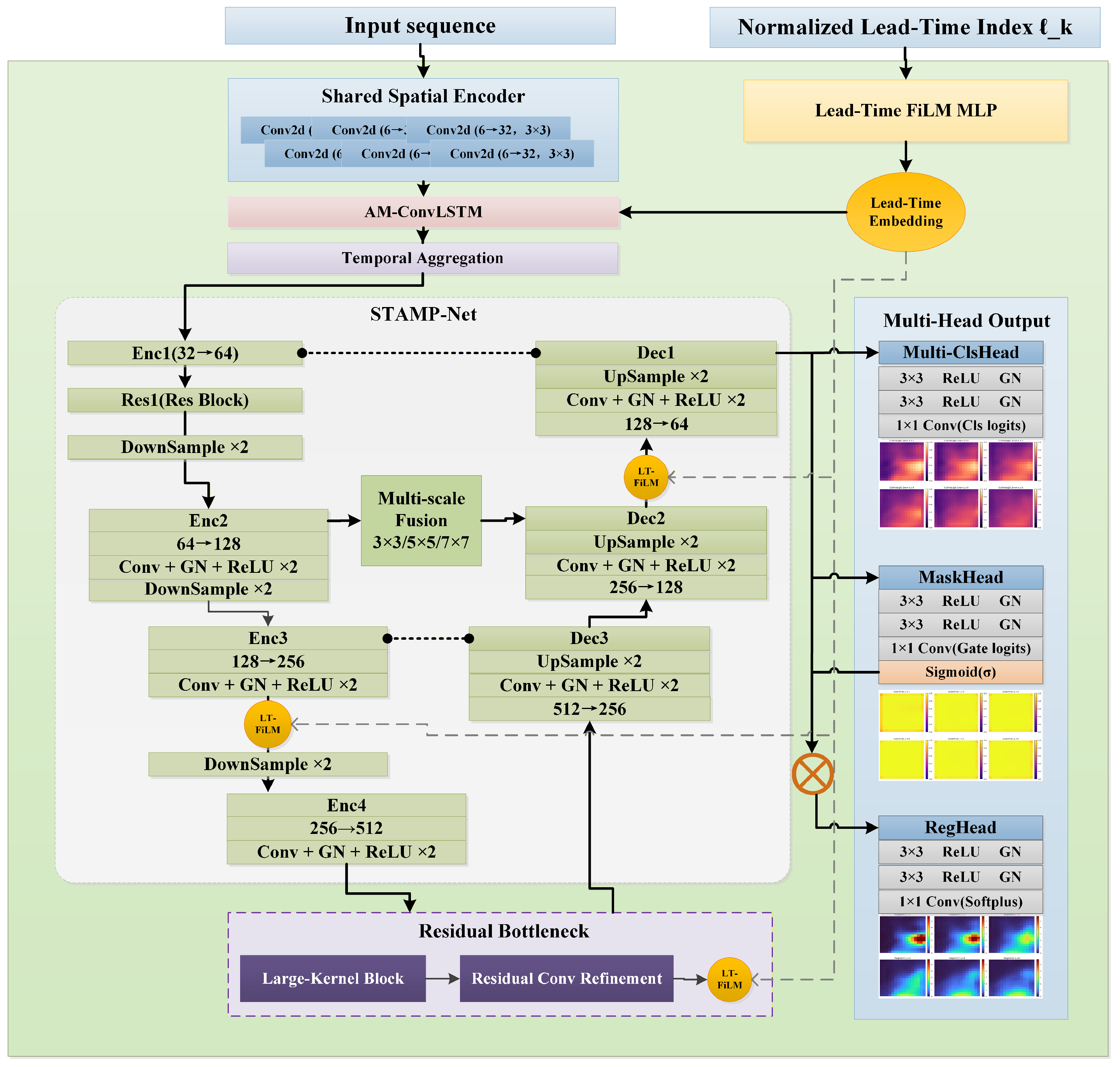
Near-surface precipitation systems exhibit spatial structures at multiple scales, ranging from broad precipitation bands to localized convective cores. These structures are difficult to represent simultaneously using a single-scale convolutional architecture. To address this issue, the STAMP-Net generator adopts a hierarchical encoder–decoder architecture with residual feature extraction, multi-scale fusion, hierarchical skip connections, and lightweight lead-time-conditioned feature modulation, as shown in Figure 3.
Taking the temporal representation F temp R C × H × W produced by the AM-ConvLSTM module as input, the encoder extracts hierarchical spatial features through progressive downsampling and residual connections. A large-kernel convolutional residual bottleneck is introduced in the deep encoder to enlarge the effective receptive field:
F b = F in + R c K l ( F in ) ,
where F in denotes the deep encoder feature map, K l ( · ) represents the large-kernel convolution operation, and R c ( · ) denotes convolutional refinement.
To represent precipitation structures at different spatial scales, the multi-scale fusion (MSF) module is introduced at intermediate encoder layers. Parallel convolutions with kernel sizes of 3 × 3 , 5 × 5 , and 7 × 7 are applied, followed by a 1 × 1 convolution for feature fusion:
F ms = Conv 1 × 1 Cat Conv 3 × 3 ( F ) , Conv 5 × 5 ( F ) , Conv 7 × 7 ( F ) ,
where F is the intermediate encoder feature map and Cat [ · ] denotes channel-wise concatenation. The parallel branches provide spatial context over different receptive-field sizes, covering both localized precipitation structures and broader precipitation regions.
The decoder restores the spatial resolution through progressive upsampling and hierarchical skip connections. High-resolution encoder features retain fine-scale spatial information, while deeper multi-scale features provide broader spatial context. Lead-time-conditioned feature modulation is applied during reconstruction so that the shared decoder can adapt its representations to different forecast positions.
To separate precipitation-occurrence identification from continuous intensity estimation at the learning-objective level, a three-head prediction structure is used at the output layer. The regression head H reg produces non-negative continuous precipitation amounts through a Softplus activation. The classification head H cls outputs logits associated with multiple precipitation-intensity thresholds and is supervised using focal loss. The occurrence-gating head H occ generates a spatial map that modulates the continuous precipitation estimate. The prediction for the k-th forecast frame is given by
Y ^ t + k = H reg ( F ) σ H occ ( F ) ,
where Y ^ t + k R H × W denotes the predicted precipitation field at lead time k, σ ( · ) is the sigmoid function, and ⊙ denotes element-wise multiplication. In this way, precipitation occurrence and continuous intensity estimation are handled by separate output branches before being combined into the final precipitation field.

2.7. AM-ConvLSTM Temporal Evolution Module

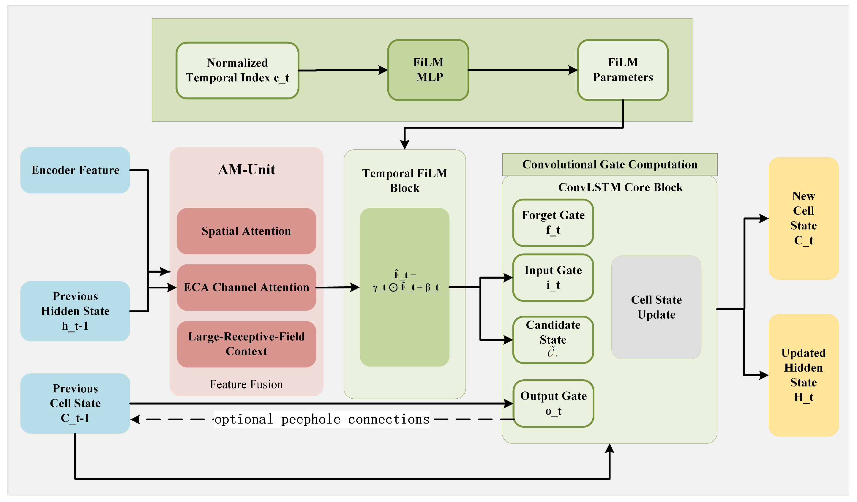
Precipitation systems evolve through successive stages of initiation, development, and decay. Standard ConvLSTM units apply shared recurrent operations to all spatial locations and channels and do not explicitly distinguish spatially relevant features or the relative position of each frame within the input sequence. To address this issue, the proposed AM-ConvLSTM module processes the shared encoder feature sequence { F 0 , t } t = 1 L using three components: an attention-augmented representation unit (AM-Unit), a temporal-index-conditioned FiLM module, and a ConvLSTM recurrent core. The resulting temporal representation F temp is subsequently passed to the STAMP-Net generator. The structure of AM-ConvLSTM is shown in Figure 4.
At each input time step t, the feature F 0 , t R C × H × W is first processed by the AM-Unit. The unit combines spatial attention, efficient channel attention (ECA) [28], and a large-receptive-field branch. Spatial attention reweights responses across spatial locations, ECA performs lightweight channel-wise recalibration, and the large-receptive-field branch provides broader spatial context than standard local convolutions. The attention-enhanced feature is written as
F ˜ t = ϕ a ( F 0 , t ) ,
where F ˜ t R C × H × W denotes the output of the AM-Unit and ϕ a ( · ) represents the composite attention mapping.
To provide the shared recurrent unit with information about the relative position of each input frame, temporal-index-conditioned feature-wise linear modulation (FiLM) is introduced. For an input sequence of length L, the normalized temporal index at time step t is defined as
c t = t 1 L 1 , t = 1 , 2 , , L .
The condition c t represents only the relative position of a frame within the input sequence; it does not encode calendar date, season, absolute time, or an explicit precipitation-dynamics mechanism. A lightweight two-layer multilayer perceptron maps c t to channel-wise scaling and shifting parameters:
( γ t , β t ) = f FiLM ( c t ) ,
where γ t , β t R C . These parameters are broadcast along the spatial dimensions and applied to the attention-enhanced feature:
F ^ t = γ t F ˜ t + β t ,
where F ^ t R C × H × W denotes the modulated feature and ⊙ represents element-wise multiplication with channel-wise spatial broadcasting. The spatially aligned two-dimensional DEM field is retained elsewhere in the model as static auxiliary geographical information; it is not spatially averaged and is not used as a FiLM conditioning variable in the final AM-ConvLSTM design.
The modulated feature F ^ t and the previous hidden state H t 1 are then passed to the ConvLSTM gating operations to compute the forget gate, input gate, candidate state, and output gate, followed by updates of the cell state C t and hidden state H t . In contrast to directly feeding the encoder feature into the recurrent core, AM-ConvLSTM applies the AM-Unit and temporal-index-conditioned modulation before the gating operations. Thus, each recurrent update receives a feature representation containing spatial attention, channel recalibration, broader spatial context, and relative sequence-position information.
Using only the final hidden state H L may discard recent temporal information distributed across the preceding recurrent states. The temporal readout module therefore retains the final three hidden states and fuses them through a learnable projection. Given the hidden-state sequence { H t } t = 1 L , the temporal representation is defined as
F temp = Φ r { H t } t = 1 L = f proj Concat c H L 2 , H L 1 , H L ,
where Concat c ( · ) denotes concatenation along the channel dimension and f proj ( · ) is a learnable 1 × 1 convolutional projection. Each hidden state has dimensions H t R C h × H × W . In the present implementation, C h = 32 , so concatenating the final three states produces a 96 × H × W tensor. The projection uses a 1 × 1 convolution with 96 input and 96 output channels, yielding F temp R 96 × H × W for subsequent processing by STAMP-Net. This operation is neither temporal average pooling nor selection of only the final hidden state.

2.8. Dual-Branch Temporal PatchGAN Discriminator

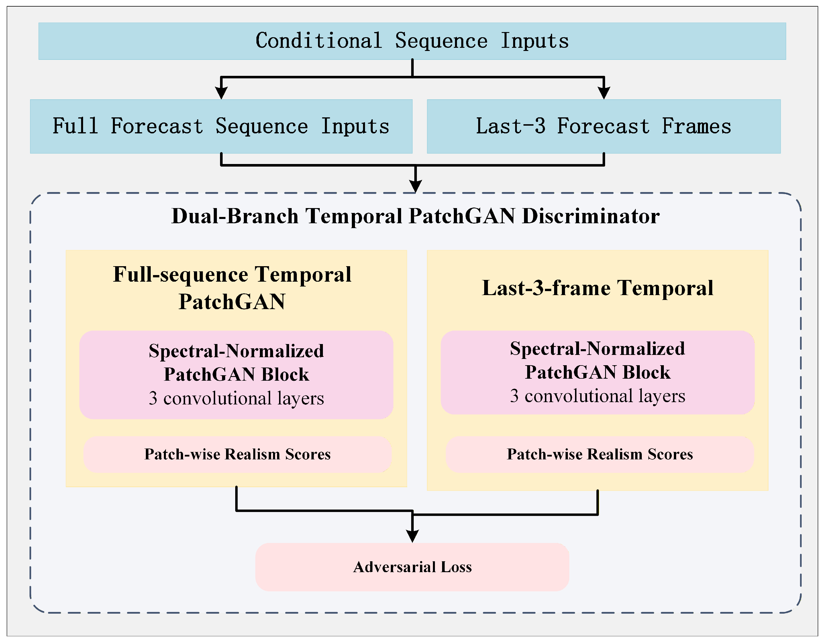
In precipitation nowcasting, forecast uncertainty increases with lead time, which may result in blurred precipitation boundaries, weakened heavy-rainfall cores, and degraded local structures in later prediction frames. Conventional temporal discriminators usually evaluate the complete forecast sequence with uniform temporal constraints and therefore provide limited supervision for specific late-stage degradation. To address this issue, a dual-branch temporal PatchGAN discriminator is introduced, consisting of a full-sequence discriminator D and a late-stage focal discriminator D last 3 , as shown in Figure 5.
The full-sequence discriminator D takes the generated sequence Y ^ , the corresponding conditional input X, and the ground-truth sequence Y as conditional adversarial inputs. It evaluates the overall realism of the predicted sequence and provides supervision for maintaining spatiotemporal consistency throughout the forecast window.
The discriminator adopts the PatchGAN formulation, which evaluates local patch-level realism rather than assigning a single score to the entire sequence. This local discrimination strategy provides constraints on spatial structures such as precipitation boundaries and localized heavy-precipitation regions. The global discriminator is optimized using the WGAN-GP objective:
L D global = E D ( Y ^ X ) E D ( Y X ) + λ gp E ( Y ˜ D 2 1 ) 2
where Y ˜ = ϵ Y + ( 1 ϵ ) Y ^ , ϵ U ( 0 , 1 ) , denotes an interpolated sample between real and generated sequences, and λ gp is the gradient penalty coefficient.
The late-stage focal discriminator D last 3 operates only on the final K = 3 frames of the prediction sequence. These frames generally contain larger accumulated forecast errors and are therefore more likely to suffer from structural degradation. By introducing an additional adversarial signal, this branch provides focused supervision for the precipitation structures and intensity distributions of later forecast frames.
The corresponding loss is defined as
L D last 3 = E D last 3 ( Y ^ last 3 X ) E D last 3 ( Y last 3 X ) + λ gp E ( Y ˜ last 3 D last 3 2 1 ) 2
where Y ˜ last 3 = ϵ Y last 3 + ( 1 ϵ ) Y ^ last 3 represents the interpolation between real and generated samples over the last three forecast frames.
The generator adversarial objective combines the signals from the two discriminator branches:
L adv = λ adv L adv global + λ adv 3 L adv last 3
where λ adv and λ adv 3 control the relative contributions of global sequence realism and late-stage structural supervision, respectively. Through this dual-branch design, the discriminator provides complementary adversarial constraints over both the complete forecast sequence and the later forecast frames.

2.9. Loss Functions

A single reconstruction loss is usually insufficient for precipitation nowcasting. Pixel-wise losses such as MSE and L1 may lead to spatially smoothed predictions, while adversarial training alone can make optimization unstable. In addition, neither type of loss explicitly constrains temporal continuity or spatial-gradient consistency. The generator is therefore trained using a hybrid objective:
L total = L reg + L cls + λ m L mask + λ adv L adv global + λ adv 3 L adv last 3 + λ t L temp + λ s L grad ,
where λ m is the occurrence-mask loss weight, λ adv and λ adv 3 control the strengths of the full-sequence and late-frame adversarial signals, respectively, λ t is the temporal-consistency weight, and λ s is the spatial-gradient consistency weight.
To impose stronger constraints on heavy precipitation regions, an intensity-dependent weight w ( Y ) is introduced:
L reg = E w ( Y ) · Y ^ Y 1
where Y ^ and Y denote the predicted and ground-truth precipitation fields, respectively, and w ( Y ) dynamically weights samples according to precipitation intensity, allowing heavy-precipitation regions, which carry the most severe operational consequences, to receive greater attention.
To address the imbalance between precipitation and non-precipitation samples, as well as the rarity of high-intensity events, a multi-threshold focal classification loss is used:
L cls = k α k FL ( M ^ k , M k ) , M k = I ( Y τ k ) ,
where τ k { 0.1 , 0.5 , 1.0 , 5.0 , 10.0 , 15.0 , 20.0 , 25.0 , 30.0 } mm h−1 denotes the set of precipitation-intensity thresholds, α k is the threshold-specific weight, and FL ( · ) is the focal loss [29].
The occurrence-gating head H occ is supervised using binary cross-entropy:
L mask = BCE σ H occ ( F ) , I ( Y τ occ ) ,
where τ occ = 0.1 mm h−1 and σ ( · ) is the sigmoid function. This term provides direct supervision for distinguishing precipitating and non-precipitating regions.
To encourage temporal continuity in the predicted sequence, abrupt inter-frame changes are penalized:
L temp = E k = 1 K 1 Y ^ t + k + 1 Y ^ t + k 1 .
This term constrains the predicted precipitation sequence to vary smoothly between adjacent lead times.
Spatial-gradient consistency is used to constrain precipitation boundaries and local spatial structures:
L grad = E Y ^ Y 1 ,
where ∇ denotes the two-dimensional spatial-gradient operator.
The adversarial terms L adv global and L adv last 3 are provided by the full-sequence and late-stage discriminators, respectively, as described in the previous subsection. Together, they provide adversarial supervision for the complete forecast sequence and the final three forecast frames. The complete set of loss weights is summarized in Table 2.
The hybrid-loss weights were determined empirically through preliminary manual tuning rather than through an exhaustive grid search or an automatic uncertainty-weighting strategy. During model development, several weight combinations were examined according to training stability and validation-set performance. The regression-related terms were treated as the main objectives for precipitation-intensity reconstruction, while the classification, gradient, and adversarial terms were used as complementary constraints for event identification and structural preservation.
The adversarial weights were intentionally set to relatively small values, 0.05 and 0.08, to reduce the risk of adversarial gradients dominating the numerical reconstruction terms. After the reported configuration was selected, all loss weights were fixed and used unchanged in the subsequent experiments. The test set was not used for loss-weight selection. These values should therefore be regarded as validation-based empirical settings rather than globally optimal weights.

2.10. Experimental Setup

2.10.1. Computational Configuration

The proposed STAMP-GAN model was implemented in PyTorch 2.8.0 and trained on a single NVIDIA RTX 4090D GPU with 24 GB of memory. Adam was used with an initial learning rate of 1 × 10 4 , a maximum of 80 epochs, and a batch size of 4. Early stopping was applied when the validation loss did not improve for 20 consecutive epochs.
The ERA5 and CMA-S configurations were trained as separate models from random initialization. The model trained on one dataset was not used to initialize, fine-tune, or evaluate the model on the other dataset. The 16 × 16 and 80 × 80 experiments therefore represent two independent applications of the same high-level STAMP-GAN framework rather than a cross-resolution transfer experiment.

2.10.2. Baseline Adaptation and Fair-Comparison Protocol

To evaluate STAMP-GAN under a common regional precipitation-forecasting setting, we selected representative recurrent, convolutional, Transformer-based, graph-based, adversarial, and diffusion-based models as comparative baselines. These include ConvLSTM [12], TrajGRU [13], U-Net++ [14], PhyDNet [15], Swin Transformer [16], DGMR [17], MetNet3-R [23], PreDiff-R [20], SpateGAN [18], GraphCast-R [22], Diffusion Nowcasting [21], and Fusion-2025 [30]. The selected methods cover several commonly used modeling strategies for spatiotemporal precipitation prediction.
ConvLSTM and TrajGRU represent recurrent spatiotemporal forecasting architectures. ConvLSTM replaces fully connected state transitions with convolutional operations, whereas TrajGRU introduces dynamically determined recurrent connections to better represent spatial motion. U-Net++ uses a nested encoder–decoder structure with dense skip connections, while PhyDNet separates learned physical dynamics from residual components through a dual-branch recurrent architecture. Swin Transformer introduces shifted-window self-attention for hierarchical spatial feature extraction. DGMR and SpateGAN represent adversarial generative approaches, and PreDiff-R and Diffusion Nowcasting represent diffusion-based forecasting approaches. These models provide comparisons across different temporal, spatial, and generative forecasting strategies.
For clarity, the suffix “-R” denotes a regional adaptation implemented for the present local-data forecasting task. GraphCast-R, MetNet3-R, and PreDiff-R should therefore not be interpreted as complete reproductions of the corresponding original large-scale systems. Instead, they retain the principal modeling ideas of the original architectures while adapting the required input, output, temporal, and spatial interfaces to the regional datasets used in this study.
MetNet3-R is a regional implementation inspired by the spatial-context modeling and probabilistic forecasting principles of MetNet-3 [23]. Its input and output interfaces were reconstructed for the regional grid and the six-step hourly forecasting task. PreDiff-R is based on the conditional latent-diffusion formulation of PreDiff [20]; its conditioning interface, spatial dimensions, and forecast output were adapted to the present regional input–output setting while retaining the conditional diffusion principle.
GraphCast-R is a regional graph-based implementation inspired by the message-passing architecture of GraphCast [22]. Because the original GraphCast system was developed for global medium-range forecasting using a multi-resolution icosahedral representation, its full configuration is not directly transferable to the present regional hourly forecasting task. Accordingly, the regional spatial grid was represented as a graph, while the input and output interfaces were adapted to the local forecasting setting. The GraphCast-R results therefore evaluate GraphCast-style graph message passing under the present regional configuration rather than the operational performance of the original GraphCast system.
All compared models were evaluated under the same regional forecasting task as STAMP-GAN. Each model used observations from the previous six-hourly time steps as input and generated precipitation forecasts for lead times of 1–6 h. ERA5 and CMA-S were treated as two independent forecasting tasks. Models were trained and evaluated separately on the corresponding datasets, and performance comparisons were conducted only among models evaluated on the same dataset. No weights, learned features, intermediate states, or normalization statistics were transferred between ERA5 and CMA-S.
Within each dataset, the chronological training, validation, and test partitions, quality-control procedures, normalization rules, test samples, forecast horizon, precipitation thresholds, and evaluation metrics were kept consistent across the compared methods. The absolute metric values obtained on ERA5 and CMA-S were not used for direct cross-dataset ranking because the two datasets differ in spatial resolution, data source, precipitation distribution, and reference-field construction.
Because the baseline models were originally developed for different spatial resolutions, input modalities, and forecasting settings, implementation changes were restricted to those required by the present regional task. These changes mainly involved the available input variables, grid dimensions, temporal input length, forecast horizon, conditioning interface, and output dimensions. Architecture-specific modeling mechanisms were retained whenever applicable.
For recurrent sequence models, including ConvLSTM, TrajGRU, and PhyDNet, the input and output interfaces were configured for six historical time steps and six future precipitation fields. For encoder–decoder and Transformer architectures, including U-Net++ and Swin Transformer, the temporal inputs were organized according to the corresponding model formulation and the output layers were adjusted to produce the required six forecast lead times. For the regional graph-based baseline, the global-domain graph representation was replaced by a graph constructed from the regional spatial grid. For adversarial and diffusion-based models, the corresponding generative or denoising mechanisms were retained while their conditioning and output interfaces were adapted to the regional forecasting task.
All compared models were trained from random initialization on the corresponding local training sets, without using official pretrained weights. Training progress, hyperparameter selection, early stopping, and checkpoint selection were determined using only the training and validation partitions, while the test partition was reserved for final evaluation. Unless otherwise specified, random seed 42 was used for the baseline experiments.
No exhaustive or automated hyperparameter search was performed. Model-specific settings, including learning rate, batch size, hidden dimensions, loss function, optimizer, and learning-rate schedule, were determined with reference to the corresponding architecture and available implementation, subject to GPU-memory constraints, numerical stability, convergence behavior, and validation-set performance. The final checkpoint for each model was selected according to validation CSI. Test-set results were not used for hyperparameter selection or checkpoint selection.
For stochastic generative baselines, including DGMR, SpateGAN, PreDiff-R, and Diffusion Nowcasting, one forecast realization was generated for each test sample and evaluated using the same deterministic verification metrics as the other models. No ensemble averaging, best-sample selection, or multi-sample post-processing was applied. This protocol provides a consistent single-realization comparison under the common regional evaluation setting, but it does not characterize the full probabilistic performance of these models. Probabilistic calibration, ensemble spread, reliability, and spread–skill relationships are therefore outside the scope of the present comparison.
Within each dataset, categorical performance was evaluated using POD, HSS, FAR, and CSI, continuous performance was evaluated using MAE, RMSE, CORR, and MBE, and neighborhood-scale spatial agreement was additionally assessed using FSS. Detailed model-specific input variables, spatial configurations, adaptations, parameter counts, stochastic sampling settings, loss functions, optimizers, learning rates, learning-rate schedules, training epochs, batch sizes, random seeds, and checkpoint-selection rules are reported in the Supplementary Materials (Tables S1 and S2).

2.10.3. Robustness Experiment for the Last-Three-Frame Discriminator

To assess the robustness of the dual-branch discriminator against the stochasticity of GAN training, the full STAMP-GAN and the variant without the last-three-frame discriminator D last 3 were independently trained using five paired random seeds, namely, 42, 123, 2024, 3407, and 5678. For each seed, the two configurations used identical data partitions, sampling procedures, optimization settings, and model-selection criteria. The only difference was that D last 3 and its associated adversarial loss term were removed from the reduced configuration. Results are reported as the mean and standard deviation over the five paired runs.

2.11. Evaluation Metrics

To comprehensively evaluate model performance across different precipitation intensity levels, this study adopts an integrated assessment framework combining categorical verification metrics and continuous regression metrics. Categorical metrics are calculated at multiple precipitation-intensity thresholds to evaluate precipitation-event detection. Because grid-point metrics may penalize small spatial displacement errors, neighborhood-based verification is additionally introduced to evaluate spatial agreement.
The critical success index (CSI) [31] is defined as
CSI = TP TP + FP + FN
where TP, FP, and FN denote true positives, false positives, and false negatives, respectively. CSI provides a balanced measure of categorical forecast skill by accounting for both missed events and false alarms. It is used as one of the primary categorical verification metrics in this study.
The probability of detection (POD) [31] and false alarm ratio (FAR) [31] are defined as
POD = TP TP + FN
FAR = FP TP + FP
POD measures the fraction of observed precipitation events that are correctly predicted, while FAR quantifies the fraction of forecast events that fail to materialize.
The Heidke skill score (HSS) [31] evaluates forecast skill relative to random chance:
HSS = 2 ( TP · TN FP · FN ) ( TP + FN ) ( FN + TN ) + ( TP + FP ) ( FP + TN )
HSS ranges from to 1, where 1 indicates perfect skill and 0 indicates no skill beyond random chance.
Because grid-point verification metrics may impose a double penalty on precipitation forecasts with small spatial displacement errors, the Fractions Skill Score (FSS) was additionally used to evaluate neighborhood-scale spatial agreement. For a precipitation threshold τ and an n × n neighborhood, the forecast and observed fractional coverages are denoted by f i ( n , τ ) and o i ( n , τ ) , respectively. The FSS is defined as
FSS ( n , τ ) = 1 i = 1 N f i ( n , τ ) o i ( n , τ ) 2 i = 1 N f i ( n , τ ) 2 + i = 1 N o i ( n , τ ) 2 .
The binary precipitation fields were first constructed using thresholds of 0.5, 5, and 10 mm h−1, after which neighborhood event fractions were calculated using 1 × 1 , 3 × 3 , and 5 × 5 windows. An FSS value closer to 1 indicates better neighborhood-scale spatial agreement. FSS was calculated separately at each forecast lead time and then averaged over T1–T6. The 1 × 1 scale corresponds to strict grid-point verification, whereas the 3 × 3 and 5 × 5 scales provide increasing tolerance to small spatial displacement errors.
For continuous precipitation fields, the mean absolute error (MAE) [32,33] and root mean square error (RMSE) [32,33] are defined as
MAE = 1 N i = 1 N | y i y ^ i |
RMSE = 1 N i = 1 N ( y i y ^ i ) 2
where y i and y ^ i denote the values at grid point i in the ground-truth precipitation field Y and the predicted field Y ^ , respectively, and N is the total number of valid grid points.
The mean bias error (MBE) [34] quantifies systematic overestimation or underestimation of precipitation fields:
MBE = 1 N i = 1 N ( y ^ i y i ) ,
where y i and y ^ i denote the observed and predicted precipitation values at grid point i, respectively, and N is the total number of valid grid points. An MBE value close to zero indicates that the model has little systematic bias. Positive MBE values indicate overestimation, whereas negative MBE values indicate underestimation.
The Pearson correlation coefficient (CORR) [32] measures the linear consistency between the predicted and observed fields:
CORR = i = 1 N ( y i y ¯ ) ( y ^ i y ^ ¯ ) i = 1 N ( y i y ¯ ) 2 i = 1 N ( y ^ i y ^ ¯ ) 2
The Kling–Gupta efficiency (KGE) [35] provides a multi-component evaluation that decomposes forecast quality into correlation, bias ratio, and variability ratio:
KGE = 1 ( r 1 ) 2 + ( α 1 ) 2 + ( β 1 ) 2
where r is the Pearson correlation coefficient, α = σ y ^ / σ y is the variability ratio, and β = μ y ^ / μ y is the bias ratio. All metrics are computed on the original, non-resampled test set to ensure objective evaluation.
In addition to the full-grid evaluation, a station-constrained sensitivity analysis was conducted for the CMA-S dataset. Grid cells located within 5 km of at least one physical rain-gauge station were retained using a fixed spatial mask. The 5 km threshold approximately corresponds to one CMA-S grid spacing and retains 80.92% of the evaluation domain. The same mask was applied to the predictions and reference fields of all evaluated models. CSI, POD, and FAR were calculated separately at each forecast lead time and then averaged over T1–T6, consistent with the primary evaluation protocol.
To evaluate the statistical robustness of CSI improvements between competing methods, paired block-bootstrap analysis was additionally performed. Two temporal block lengths (24 h and 72 h) were considered to evaluate the sensitivity of the estimated confidence intervals. The complete paired block-bootstrap confidence intervals are reported in the Supplementary Materials (Table S3).

3. Results

3.1. Ablation Study

The ablation analysis consists of four parts. First, a progressive component ablation evaluates the cumulative changes obtained by sequentially adding the main components of STAMP-GAN. Second, a removal-based ablation starts from the full model and removes each major component individually. Third, a paired multi-seed experiment is conducted to examine the robustness of the last-three-frame discriminator. Finally, different DEM usage strategies are compared to distinguish the effect of the spatially explicit two-dimensional DEM input from that of the regional-mean DEM condition.

3.1.1. Progressive Component Ablation

To examine the cumulative performance changes associated with the progressive incorporation of the principal model components, ablation experiments were conducted on the ERA5-based dataset with the auxiliary two-dimensional DEM input. Starting from a baseline model, the following components were added sequentially: the STAMP-Net generator with multi-scale spatial reconstruction, the AM-ConvLSTM temporal-modeling module, the dual-branch discriminator, and the hybrid loss formulation. All configurations used the revised DEM strategy, in which the spatially aligned two-dimensional DEM field was retained as a static auxiliary input and the regional-mean DEM condition was removed from FiLM. Unless otherwise stated, categorical metrics were calculated at the 0.5 mm h−1 precipitation threshold and averaged over forecast lead times T1–T6.
Table 3 summarizes the progressive ablation results. Because the components were introduced sequentially, the differences among configurations should be interpreted as cumulative and order-dependent changes rather than as fully independent estimates of individual component effects.
Adding STAMP-Net improves CSI from 0.5998 to 0.6193 and increases POD from 0.5359 to 0.8406. FAR decreases from 0.3597 to 0.2984, and the regression errors also decrease, with MAE reduced from 0.4799 to 0.4502 and RMSE reduced from 1.8165 to 1.1459. These changes indicate that the multi-scale spatial generator improves precipitation-event detection and reduces average prediction error relative to the baseline. CORR also increases from 0.4855 to 0.5431, although KGE decreases from 0.3804 to 0.3427, suggesting that the improvement is not uniform across all continuous metrics.
Introducing AM-ConvLSTM further increases CSI from 0.6193 to 0.6232 and slightly increases POD from 0.8406 to 0.8442. FAR decreases marginally from 0.2984 to 0.2961, and MAE decreases from 0.4502 to 0.4365. CORR and KGE also increase to 0.5558 and 0.4535, respectively. RMSE, however, increases from 1.1459 to 1.2828. These results suggest that the temporal-evolution module improves event detection, average absolute error, and correlation-based performance, while also introducing some sensitivity to larger errors.
Adding the dual-branch discriminator increases CSI from 0.6232 to 0.6333 and POD from 0.8442 to 0.8689. FAR decreases from 0.2961 to 0.2560, while MAE and RMSE decrease to 0.4274 and 1.0587, respectively. MBE also moves closer to zero, changing from 0.0431 to 0.0258 . These results indicate that, in the progressive setting, the dual-branch discriminator is associated with improved event detection and reduced error. Because this comparison comes from a single sequential ablation run, the robustness of the last-three-frame discriminator is examined separately in Section 3.1.3.
The full configuration with the hybrid loss gives the best overall balance among the progressive ablation settings. CSI increases to 0.6379, POD reaches 0.9350, and FAR decreases to 0.2495. MAE and RMSE are further reduced to 0.3892 and 0.9260, respectively, while CORR and KGE increase to 0.6180 and 0.5866. MBE is also close to zero, with a value of 0.0026. These results suggest that the hybrid loss helps balance precipitation-event detection, intensity regression, and overall field consistency.
Overall, the progressive ablation results show cumulative improvements after the main components are added sequentially. However, because the configurations are order-dependent, these results should not be interpreted as fully isolated component contributions. The specific effect of D last 3 is therefore examined using paired multi-seed experiments in Section 3.1.3, and the effects of different DEM usage strategies are analyzed separately in Section 3.1.4.

3.1.2. Removal-Based Component Ablation

Table 4 shows the effect of removing each major component from the full STAMP-GAN model. Removing the dual-branch discriminator decreases CSI from 0.6379 to 0.6272 and POD from 0.9350 to 0.8850, while FAR, MAE, and RMSE increase. This indicates that the discriminator design contributes to event detection and adversarial supervision, although the robustness of this effect is examined separately through the multi-seed analysis in Section 3.1.3.
Removing STAMP-Net leads to lower CSI, POD, CORR, and KGE, together with a substantially larger RMSE. This suggests that the multi-scale generator is important for stable spatial reconstruction. This configuration gives a slightly lower MAE than the full model, but its weaker CSI, POD, RMSE, CORR, and KGE indicate that lower average absolute error alone does not imply better event detection or better overall field consistency.
Removing AM-ConvLSTM also reduces CSI, POD, CORR, and KGE, while increasing FAR, MAE, and RMSE. This result supports the role of temporal-evolution modeling in the proposed framework. Finally, removing the hybrid loss produces the highest FAR and lower CSI, CORR, and KGE than the full model, indicating that the hybrid objective helps balance precipitation occurrence detection, intensity regression, and spatial-structure preservation.
Because the dual-branch discriminator is designed to provide additional supervision for later forecast frames, its lead-time dependence is further examined through the T1–T6 and T4–T6 multi-seed analysis in Section 3.1.3. This lead-time-focused evaluation complements the removal-based ablation by examining whether the effect of D last 3 is more evident in the final three forecast frames.

3.1.3. Multi-Seed Robustness Analysis of the Last-Three-Frame Discriminator

Because GAN training is sensitive to random initialization and stochastic optimization, the small performance difference observed in a single ablation run may not be sufficient to assess the robustness of an additional discriminator branch. Therefore, the full STAMP-GAN and the reduced configuration without D last 3 were trained using five paired random seeds. All experimental settings were kept identical except for the removal of the last-three-frame discriminator and its associated adversarial loss.
As shown in Table 5, when averaged over all six forecast lead times, the full model achieved CSI values of 0.6343 ± 0.0040 , 0.2931 ± 0.0070 , and 0.1455 ± 0.0084 at thresholds of 0.5, 5, and 10 mm h−1, respectively. These values are higher than those of the configuration without D last 3 , which obtained 0.6294 ± 0.0052 , 0.2568 ± 0.0095 , and 0.1304 ± 0.0062 .
For the final three lead times, the full model obtained T4–T6 CSI values of 0.5811 ± 0.0068 , 0.1995 ± 0.0081 , and 0.0604 ± 0.0067 , compared with 0.5777 ± 0.0056 , 0.1699 ± 0.0056 , and 0.0383 ± 0.0059 for the model without D last 3 . The full model achieved higher T4–T6 CSI for all five paired seeds at all three thresholds, indicating directionally consistent improvements in the later forecast frames. Nevertheless, the exact two-sided Wilcoxon signed-rank tests did not reach the conventional 0.05 significance level. Therefore, the last-three-frame discriminator is interpreted as a task-specific late-frame supervision mechanism rather than as an independently proven source of statistically significant quantitative improvement.

3.1.4. Ablation of DEM Usage Strategies

To distinguish the effects of the spatially explicit two-dimensional DEM input and the regional-mean DEM condition, three configurations are compared. The original DEM-conditioning configuration retains both the two-dimensional DEM input and the regional-mean DEM condition used in FiLM. The revised model retains the two-dimensional DEM input but removes the regional-mean DEM condition. The revised model without DEM input removes both the two-dimensional DEM input and the DEM-mean condition. All other network components, data partitions, training settings, and evaluation procedures are kept unchanged.
The results in Table 6 show that removing the regional-mean DEM condition while retaining the spatially explicit two-dimensional DEM input provides the best overall balance among the three DEM usage strategies. Compared with the original DEM-conditioning configuration, the revised model increases CSI from 0.6267 to 0.6379 and POD from 0.9284 to 0.9350, while reducing FAR from 0.2695 to 0.2495. MBE moves closer to zero, decreasing from 0.0450 to 0.0026, and the error metrics also improve, with MAE decreasing from 0.4331 to 0.3892 and RMSE decreasing from 0.9950 to 0.9260. CORR and KGE increase from 0.6021 and 0.5557 to 0.6180 and 0.5866, respectively. These changes indicate that the revised DEM usage strategy improves the balance among event detection, bias reduction, regression accuracy, and overall field consistency.
Because the study domain is fixed, the regional-mean DEM value remains nearly constant across samples and therefore provides limited sample-specific conditioning information. Compressing the complete terrain field into a single scalar also removes spatial elevation differences among mountainous, hilly, and coastal regions. As a result, the regional-mean DEM condition acts mainly as a sample-invariant conditioning term rather than as an informative representation of local terrain heterogeneity.
Compared with removing the DEM input entirely, retaining the two-dimensional DEM field produces higher CSI and POD, lower FAR, lower MBE, lower MAE, lower RMSE, higher CORR, and higher KGE. This indicates that the spatially explicit DEM field provides useful auxiliary geographical information even without the regional-mean conditioning. Accordingly, the regional-mean DEM condition was removed from the final model, while the spatially aligned two-dimensional DEM field was retained as a static auxiliary input channel.

3.2. Overall Comparison on the ERA5 Dataset

Categorical Verification Results on ERA5

Table 7 presents the threshold-based categorical verification results on the ERA5 test dataset. CSI, POD, and FAR are reported at precipitation thresholds of 0.5, 5, and 10 mm h−1 to evaluate model performance across light, moderate, and heavier precipitation events.
STAMP-GAN obtains the highest CSI at all three precipitation thresholds, with values of 0.6379, 0.2981, and 0.1551, respectively. As the precipitation threshold increases, the forecasting task becomes progressively more challenging for all models, resulting in lower absolute values of the categorical metrics. Nevertheless, STAMP-GAN maintains the highest CSI across all evaluated thresholds. At 5 mm h−1, STAMP-GAN attains a POD of 0.5403, outperforming the second-best model, PhyDNet, with a POD of 0.4574. At 10 mm h−1, STAMP-GAN achieves a POD of 0.3655, compared with 0.2294 for PhyDNet. These results indicate that STAMP-GAN retains a clearer performance margin over the competing methods for moderate-to-heavy precipitation events, although the absolute values of the evaluation metrics decrease as the precipitation threshold increases. STAMP-GAN also achieves the lowest FAR at all thresholds, with values of 0.2495, 0.5201, and 0.6990, indicating that the improved event-detection capability is achieved without a corresponding increase in false alarms.
Table 8 further summarizes the statistical verification results on the ERA5 dataset. STAMP-GAN achieves the highest HSS values at all three precipitation thresholds, with scores of 0.6158, 0.4088, and 0.2386 at 0.5, 5, and 10 mm h−1, respectively. In terms of continuous metrics, STAMP-GAN obtains the lowest MAE (0.3892) and the smallest absolute MBE (0.0026), indicating accurate intensity reconstruction with limited systematic bias. It also achieves competitive RMSE (0.9260) and correlation coefficient (0.6180), demonstrating balanced performance in error control and field consistency.
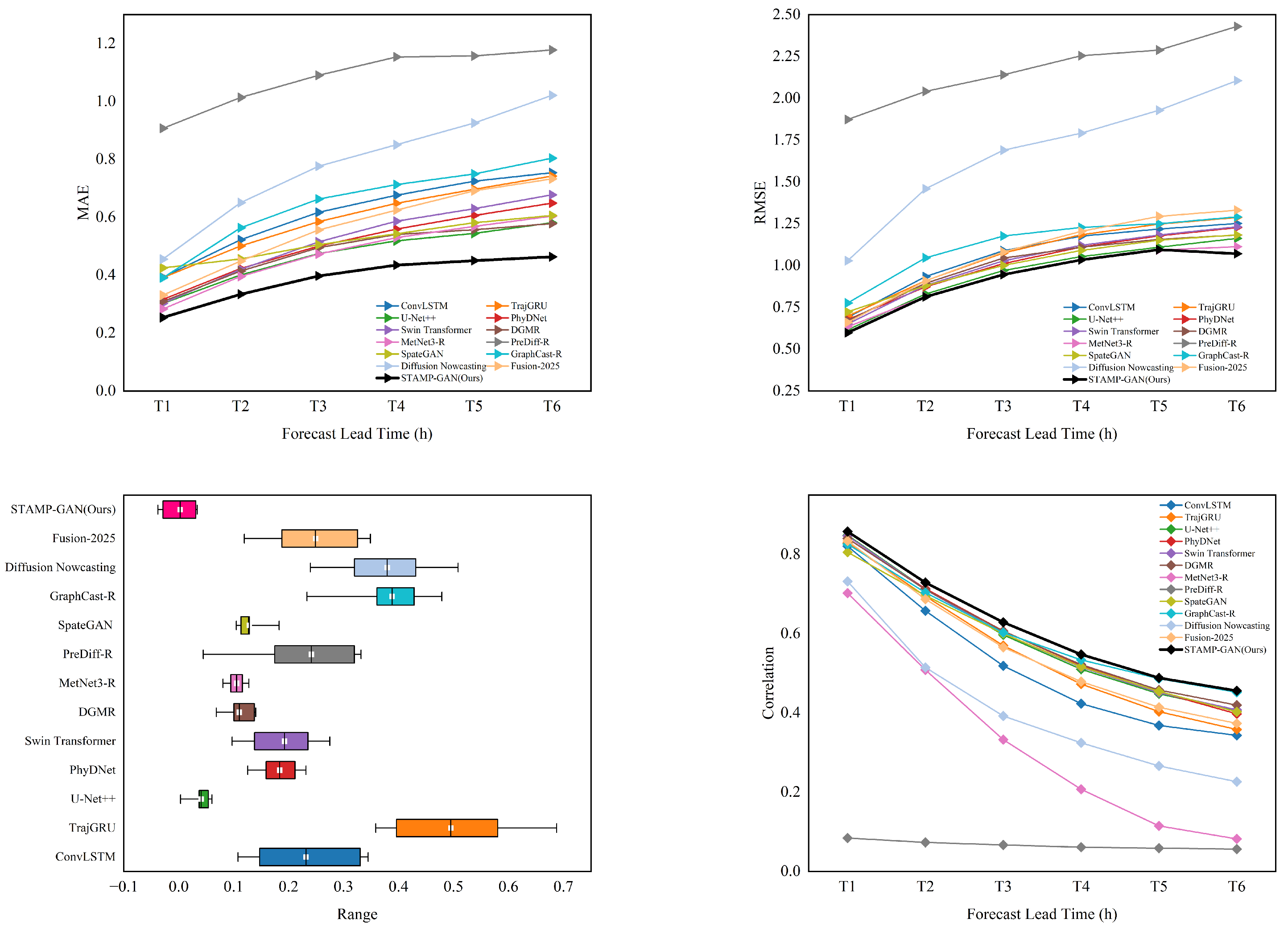
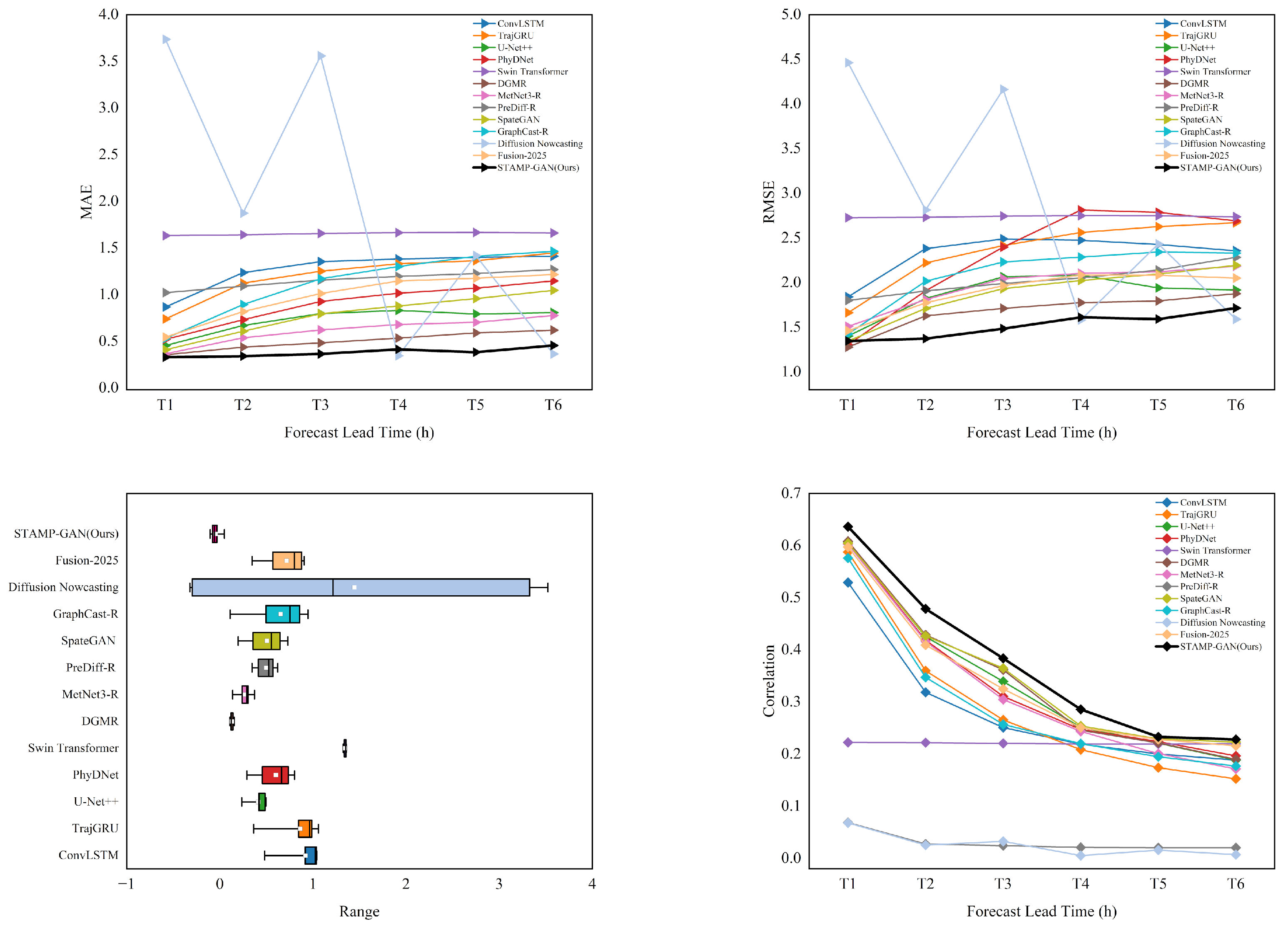
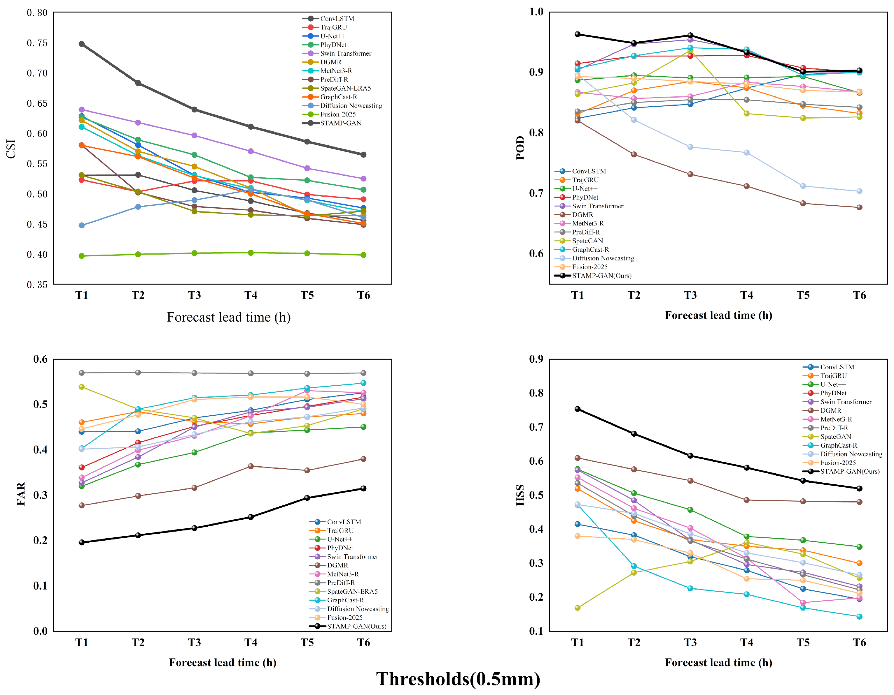
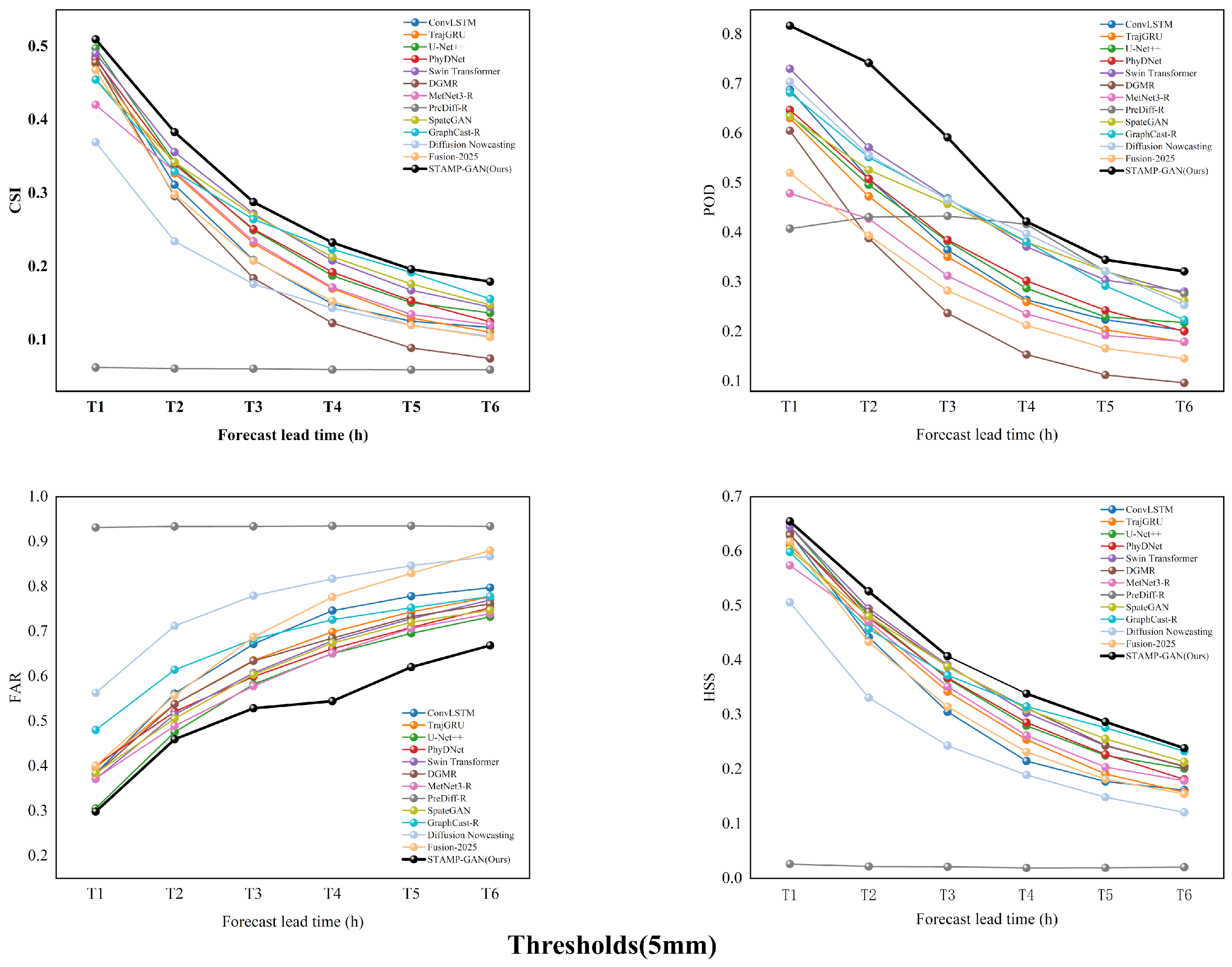
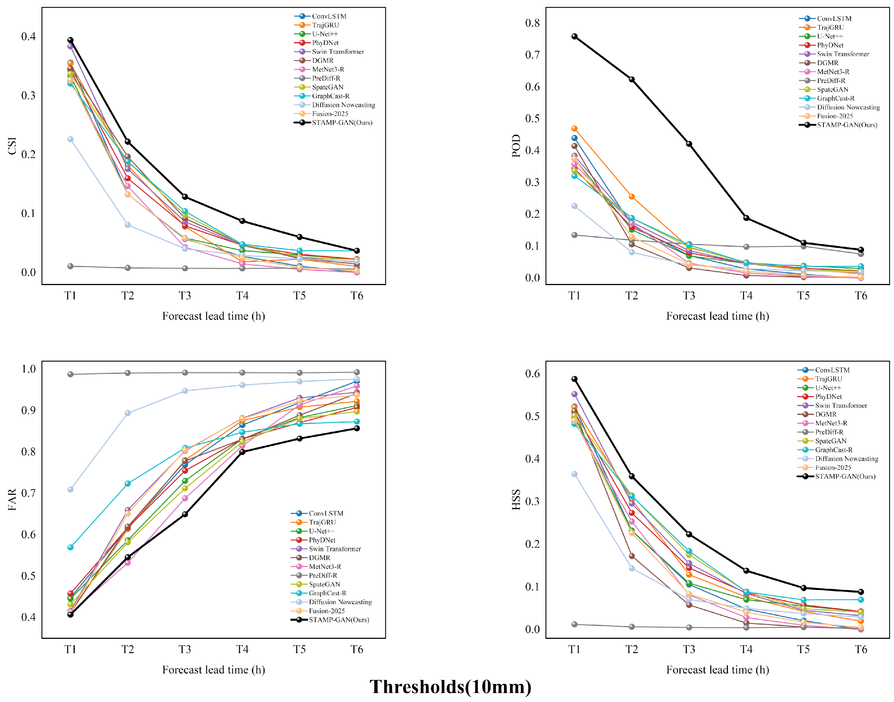
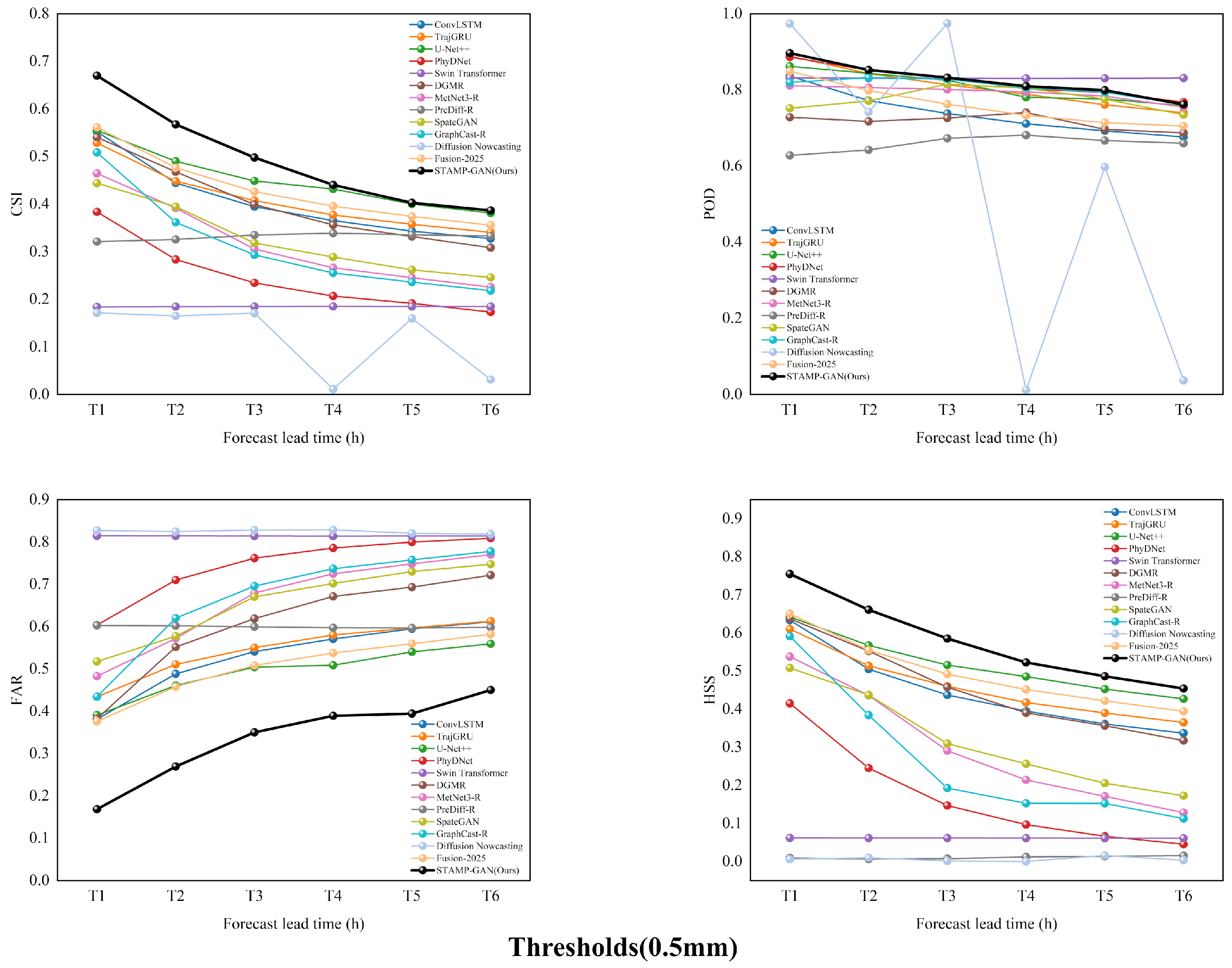
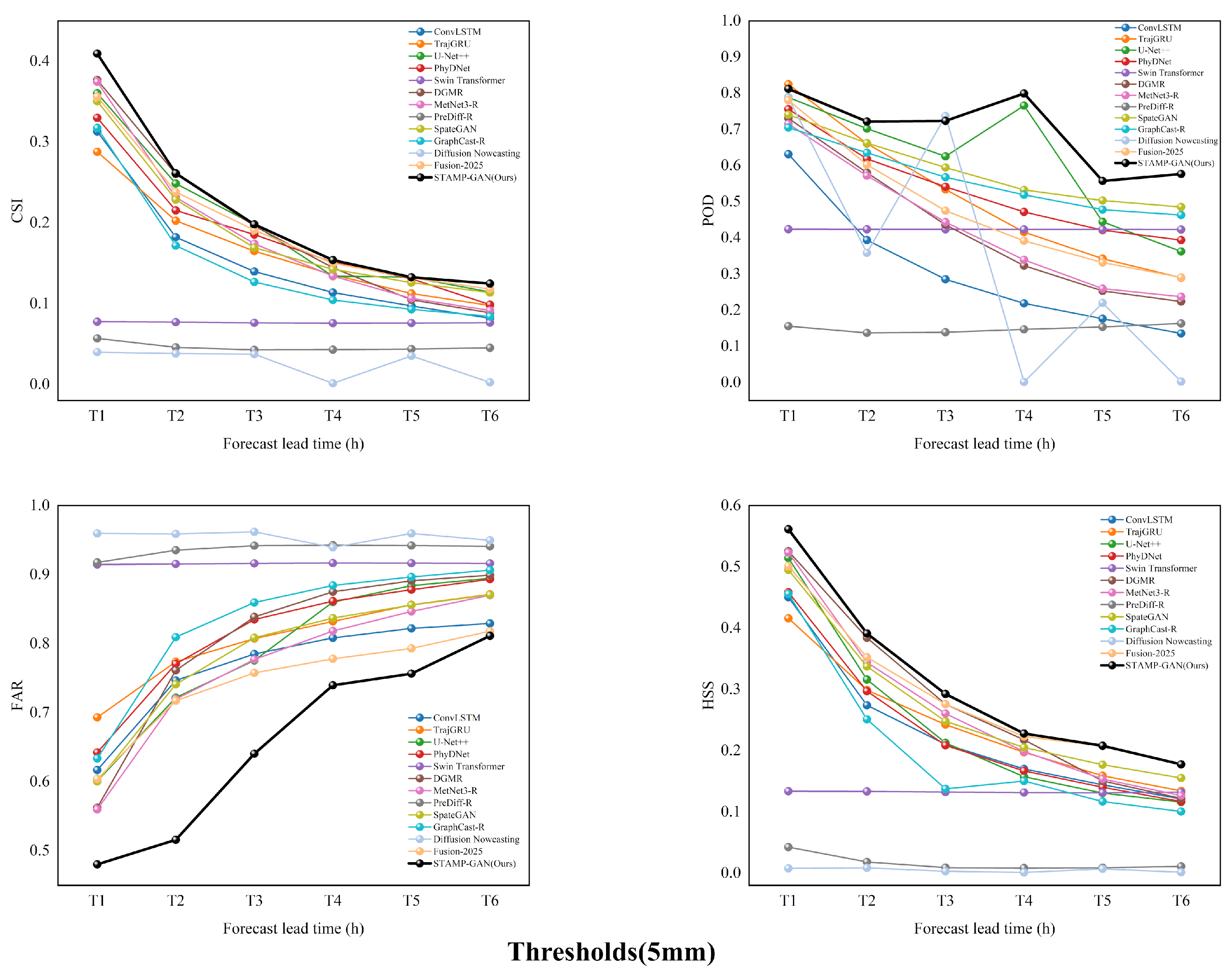
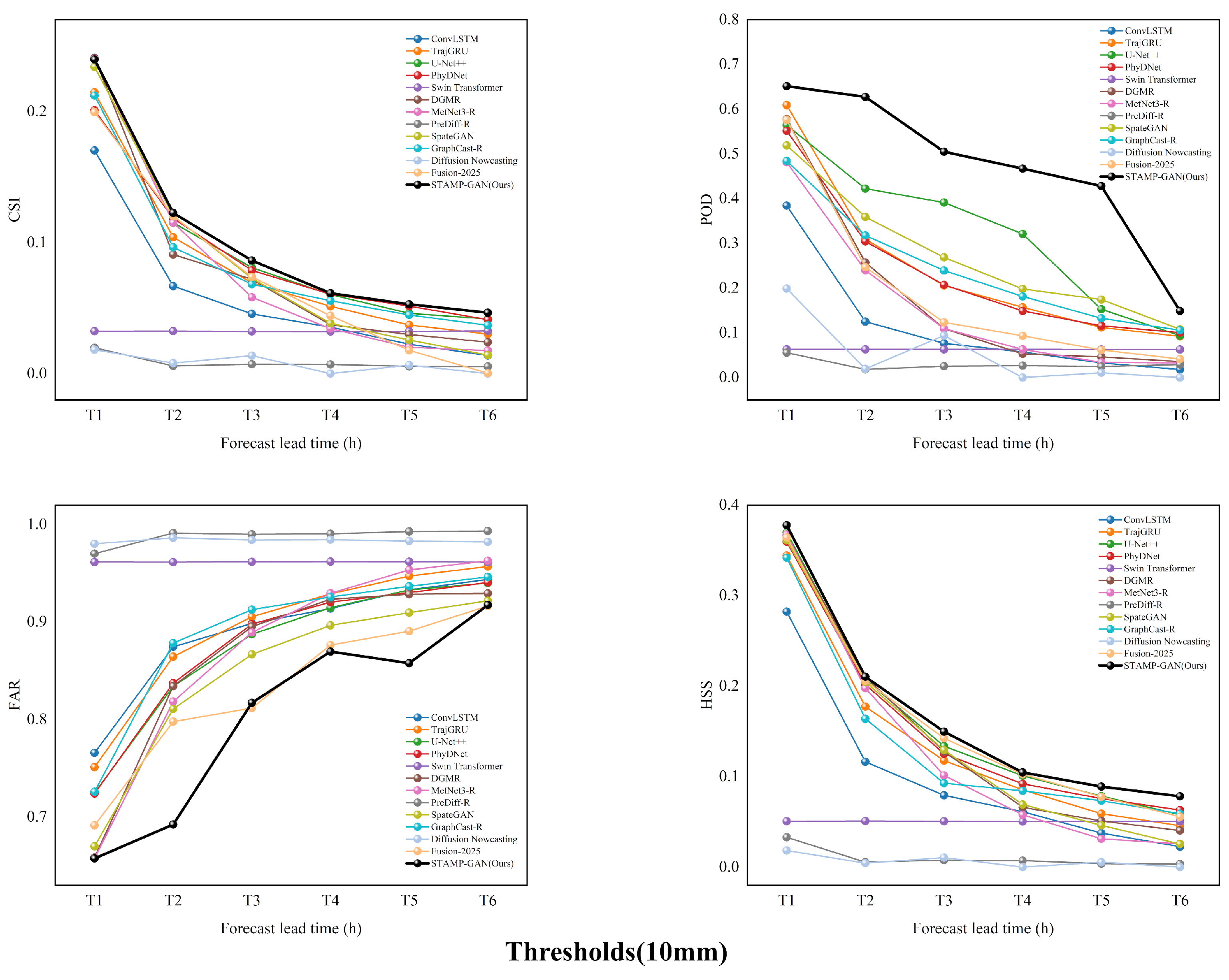
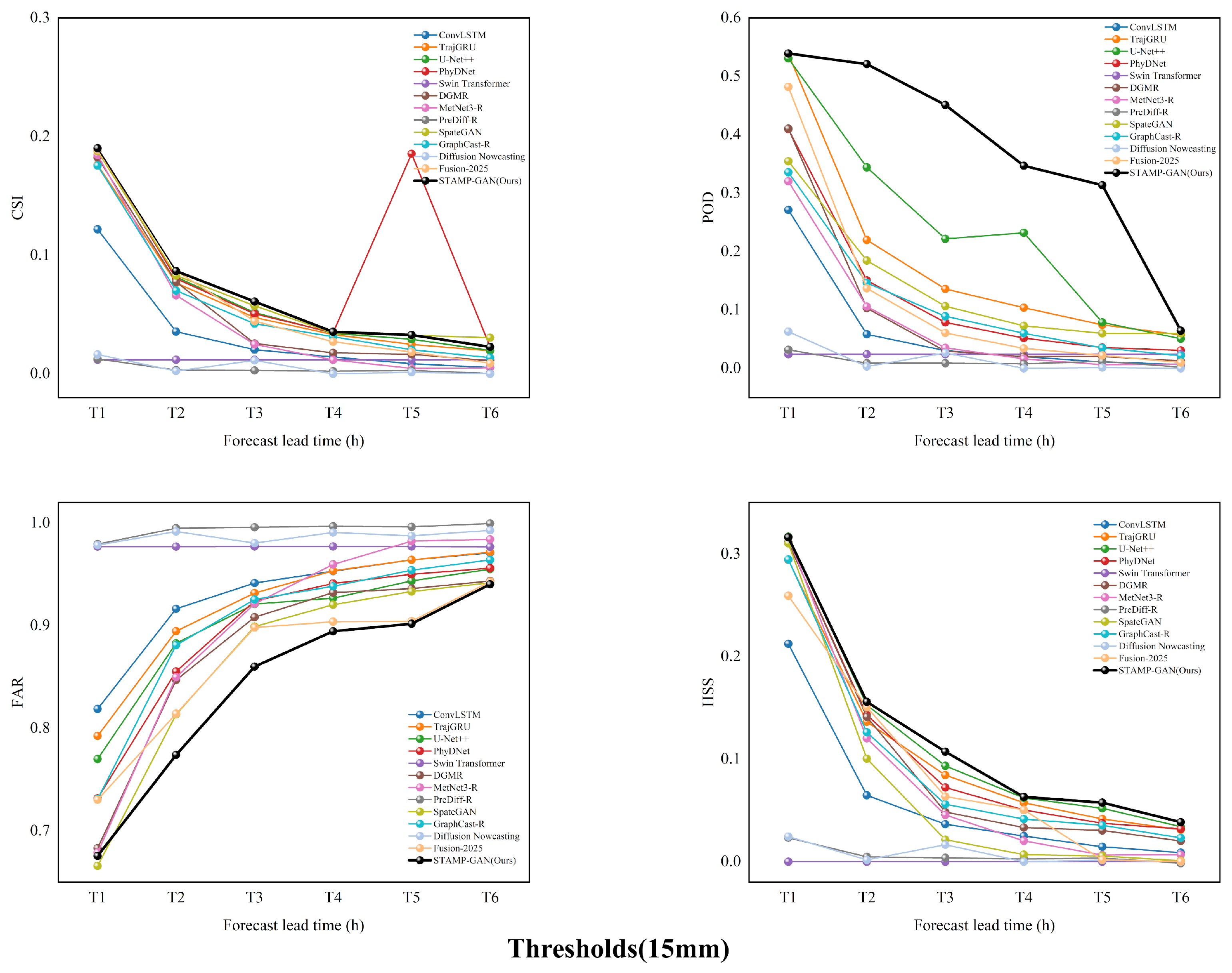
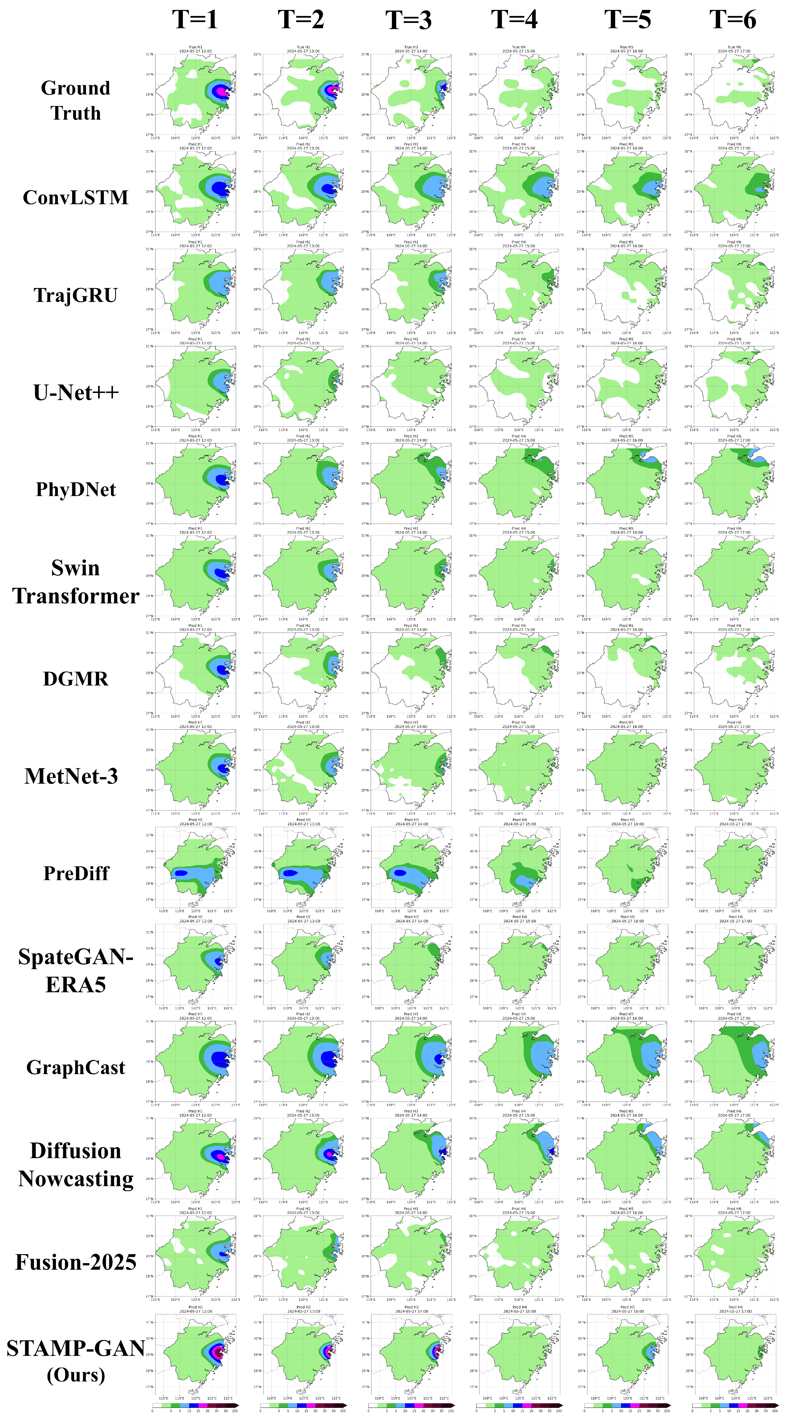
Lead-time-resolved categorical and regression metrics are shown in Figure 6, Figure 7, Figure 8 and Figure 9.
Figure 6, Figure 7, Figure 8 and Figure 9 show the lead-time-resolved categorical and regression metrics over T1–T6. STAMP-GAN generally maintains higher CSI, POD, and HSS than the baseline models across most lead times and thresholds, while its FAR remains relatively low. The separation between STAMP-GAN and the compared models becomes more visible at later lead times. This trend may be related to the combined effects of multi-scale spatial reconstruction, temporal-evolution modeling, the hybrid loss design, and the late-frame adversarial supervision.
At the 0.5 mm h−1 threshold, the CSI of STAMP-GAN decreases gradually from approximately 0.74 at T = 1 to approximately 0.56 at T = 6 , indicating a relatively slow decline in categorical skill. At the 5 mm h−1 threshold, the FAR of STAMP-GAN remains below 0.65 at T = 6 , whereas most baselines exceed 0.80 by T = 4 . This suggests that the final model maintains better false-alarm control under stricter intensity thresholds. At the 10 mm h−1 threshold, several models show very high FAR values at later lead times, indicating that high-intensity precipitation remains difficult to predict accurately.
Among the baseline models, conventional recurrent architectures, including ConvLSTM and TrajGRU, perform reasonably well at the light-precipitation threshold but degrade at higher thresholds. The evaluated diffusion-based baselines, including PreDiff-R and Diffusion Nowcasting, obtain relatively low CSI values under the adopted single-realization deterministic evaluation protocol. This result should be interpreted as regional deterministic forecasting performance rather than as a complete evaluation of their probabilistic forecasting capability.
The regional adaptations of large-scale models, including GraphCast-R and MetNet3-R, show comparatively limited performance in the present hourly regional nowcasting task. This result may reflect the mismatch between the spatial and temporal regimes for which the original architectures were developed and the substantially smaller local training domain considered here. It should therefore be interpreted as the performance of the present regional implementations rather than that of the original operational systems. Notably, SpateGAN is also evaluated under the same ERA5-based regional task setting and achieves a CSI of 0.4781 at the 0.5 mm h−1 threshold, which is lower than the 0.6379 achieved by STAMP-GAN. This comparison suggests that the observed gain is not solely due to the ERA5-based input setting.
In summary, STAMP-GAN achieves the strongest categorical forecasting skill on the ERA5 dataset and the lowest MAE among all compared models. The results indicate consistent advantages in event detection and false-alarm control across precipitation-intensity levels and forecast lead times.

3.3. Overall Comparison on the CMA-S Dataset

3.3.1. Categorical Verification Results

Table 9 and Table 10 present the threshold-based categorical verification results on the CMA-S dataset at five precipitation-intensity thresholds: 0.5, 5, 10, 15, and 20 mm h−1. Compared with ERA5, the higher spatial resolution of CMA-S ( 0.05 , 80 × 80 grid) allows evaluation at the 15 and 20 mm h−1 thresholds. These high thresholds are used to examine heavier precipitation events, but the results should be interpreted together with event rarity and the uncertainty associated with the IDW-derived reference field.
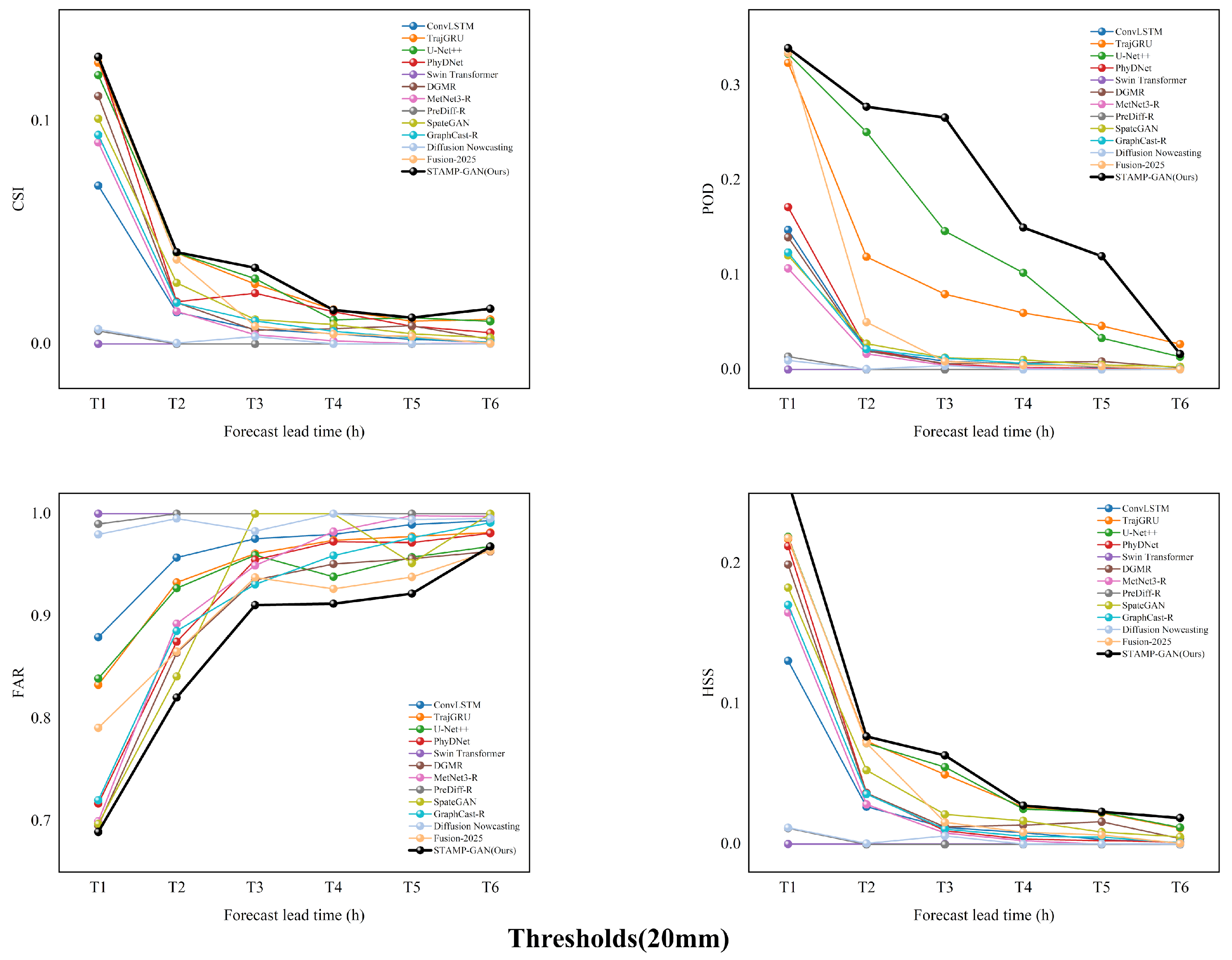
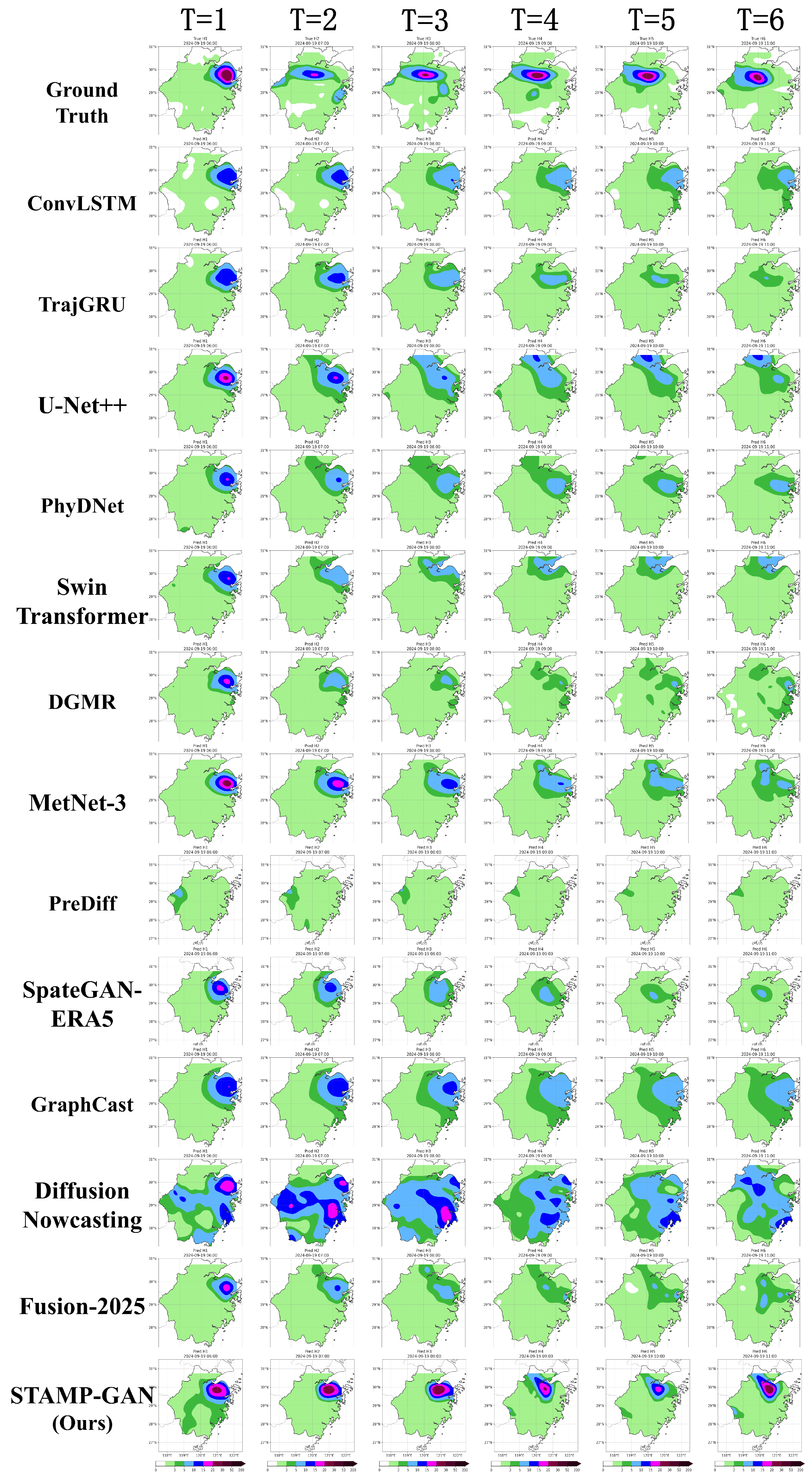
According to Table 9 and Table 10, STAMP-GAN obtains the highest CSI at the 0.5, 5, 10, and 15 mm h−1 thresholds, with values of 0.4941, 0.2134, 0.1016, and 0.0715, respectively. At the 20 mm h−1 threshold, TrajGRU obtains the highest CSI of 0.0421, while STAMP-GAN ranks second with a CSI of 0.0412. For POD, STAMP-GAN achieves the highest values at the 5, 10, 15, and 20 mm h−1 thresholds, whereas PhyDNet and Swin Transformer show slightly higher POD at the 0.5 mm h−1 threshold. These results indicate that STAMP-GAN maintains competitive categorical performance across precipitation-intensity levels, although its advantage at the 15 and 20 mm h−1 thresholds is metric-dependent. In particular, STAMP-GAN achieves substantially higher POD and lower FAR than U-Net++ at the high-intensity thresholds, whereas the CSI differences between the two models are limited. Therefore, the CMA-S results primarily demonstrate enhanced high-intensity event detection and false-alarm control rather than uniform superiority across all categorical metrics.
For FAR and HSS, STAMP-GAN shows a favorable overall balance. It obtains the lowest FAR at all five thresholds and the highest HSS from 0.5 to 15 mm h−1. At 20 mm h−1, TrajGRU achieves the highest HSS, whereas STAMP-GAN ranks second. These results indicate that STAMP-GAN remains competitive across precipitation-intensity levels. However, the high-threshold results are metric-dependent and should not be interpreted as uniform superiority across all categorical metrics.
Because the 15 and 20 mm h−1 thresholds correspond to rare heavy-precipitation events in the CMA-S test set, the high-threshold categorical scores were further examined using contingency-table counts. As reported in Table 18, the number of observed events decreases substantially as the threshold increases. For STAMP-GAN, accumulated over T1–T6, the observed event counts decrease from 1,350,982 at 10 mm h−1 to 708,830 at 15 mm h−1 and 287,419 at 20 mm h−1. These results show that the 15 and 20 mm h−1 scores are based on much smaller event samples and are therefore more sensitive to individual hits, misses, and false alarms than lower-threshold scores.
Paired block-bootstrap uncertainty analysis was further extended to the CMA-S high-threshold CSI differences between STAMP-GAN and Fusion-2025. As shown in the Supplementary Materials (Table S3), at 15 mm h−1, the CSI difference is small and the 95% confidence intervals overlap zero for both 24 h and 72 h block lengths, indicating that the 15 mm h−1 advantage should be interpreted cautiously. At 20 mm h−1, the CSI difference remains positive and the 95% confidence intervals exclude zero under both block lengths, suggesting a more stable positive difference at the rarest threshold evaluated here. Nevertheless, because the event sample is much smaller at this threshold, the 20 mm h−1 result should still be interpreted together with the contingency-table counts.
Station-Proximity Sensitivity Analysis for High-Intensity Precipitation
To examine whether the CMA-S high-threshold results are sensitive to station-to-grid interpolation and station-density effects, we repeated the evaluation using only grid cells located within 5 km of at least one physical rain-gauge station. This distance approximately corresponds to one CMA-S grid spacing and retains 5179 of the 6400 grid cells, accounting for 80.92% of the evaluation domain. U-Net++ was selected for this station-proximity comparison because it provides highly competitive high-threshold CSI among the baseline models at the 15 and 20 mm h−1 thresholds. The results are summarized in Table 11.
Restricting the evaluation to station-constrained grid cells generally increases CSI and reduces FAR for both models. At 15 mm h−1, STAMP-GAN obtains a higher POD and a lower FAR than U-Net++, whereas U-Net++ obtains a higher CSI. A similar pattern is observed at 20 mm h−1. These results suggest that the high-intensity advantage of STAMP-GAN on the CMA-S dataset is mainly reflected in higher detection sensitivity and lower false-alarm ratio, rather than in uniformly higher CSI. The station-constrained analysis therefore supports a more cautious interpretation of the CMA-S high-threshold results.

3.3.2. Continuous Verification Results

In terms of continuous metrics (Table 12), STAMP-GAN obtains the lowest MAE and RMSE and has an MBE close to zero. It also achieves the highest correlation coefficient. These results indicate lower overall intensity error and limited systematic bias on the CMA-S test set.

3.3.3. Lead-Time-Resolved Results

Lead-time-resolved categorical and regression metrics on the CMA-S dataset are shown in Figure 10, Figure 11, Figure 12, Figure 13, Figure 14 and Figure 15.
Figure 10, Figure 11, Figure 12, Figure 13, Figure 14 and Figure 15 present the lead-time-resolved performance on the CMA-S dataset. At the 0.5 mm h−1 threshold, STAMP-GAN maintains higher CSI than the compared models across most lead times, while its FAR remains relatively low. At the 5 and 10 mm h−1 thresholds, the advantage remains visible for several lead times, although the categorical scores decrease as the threshold increases.
At the 15 and 20 mm h−1 thresholds, the lead-time curves fluctuate more strongly because the number of observed events is much smaller. STAMP-GAN generally maintains higher POD and lower FAR than most compared models, but the CSI differences are limited and vary with lead time. These results are consistent with the table-based analysis and support a cautious interpretation of high-intensity precipitation skill on the IDW-derived CMA-S reference field.
For the regression metrics shown in Figure 15, STAMP-GAN generally maintains lower MAE and RMSE across the six lead times. Its MBE remains close to zero compared with most baselines, indicating limited systematic bias in the overall precipitation fields.
In summary, the CMA-S results indicate that STAMP-GAN performs competitively under the higher-resolution station-interpolated evaluation setting. Its main advantages are reflected in event detection, false-alarm control, and overall intensity-error reduction. For the 15 and 20 mm h−1 thresholds, the results should be interpreted together with the event-count statistics, bootstrap uncertainty analysis, and station-proximity sensitivity analysis because these scores are affected by event rarity and the IDW-derived reference field. Because the present evaluation covers only one rainy season, the paired block-bootstrap analysis is intended to quantify sampling uncertainty rather than eliminate the limitation of limited temporal coverage. Evaluation over multiple years will be included in future work to further assess long-term robustness.

3.4. Neighborhood-Based Spatial Verification

Grid-point verification metrics such as CSI, MAE, and RMSE are sensitive to small spatial displacement errors. A spatially coherent precipitation system may therefore receive a relatively large penalty when its predicted location is slightly shifted from the reference field. To provide a complementary spatially tolerant evaluation, the Fractions Skill Score (FSS) was calculated at precipitation thresholds of 0.5, 5, and 10 mm h−1 using 1 × 1 , 3 × 3 , and 5 × 5 neighborhoods. For each threshold, the continuous precipitation fields were first converted into binary event fields, after which, neighborhood event fractions were calculated. FSS was computed separately at each forecast lead time and then averaged over T1–T6. The results for ERA5 and CMA-S are reported in Table 13 and Table 14, respectively.
On the ERA5 dataset, STAMP-GAN obtains the highest FSS across all evaluated precipitation thresholds and neighborhood sizes. At the 0.5 mm h−1 threshold, its FSS increases from 0.771 at the 1 × 1 scale to 0.934 at the 5 × 5 scale. At 5 mm h−1, the corresponding values are 0.439, 0.663, and 0.759, while at 10 mm h−1 they are 0.227, 0.424, and 0.527. These results indicate that the performance advantage of STAMP-GAN on ERA5 is retained not only at the strict 1 × 1 grid-point scale but also under the more spatially tolerant 3 × 3 and 5 × 5 neighborhood settings.
On the CMA-S dataset, STAMP-GAN obtains the highest FSS at all three neighborhood sizes for the 0.5 and 5 mm h−1 thresholds. At 10 mm h−1, it ranks first at the 1 × 1 and 3 × 3 scales, with FSS values of 0.341 and 0.367, respectively. At the 5 × 5 scale, PreDiff-R obtains the highest FSS of 0.423, while STAMP-GAN ranks second with 0.408. These results show that the favorable performance of STAMP-GAN is also present under neighborhood-based verification, although the model ranking varies with precipitation intensity and neighborhood size on CMA-S.

3.5. Case Studies

To provide a qualitative illustration of the spatial forecast characteristics of the compared models, two representative precipitation events from the ERA5 test set were selected. Figure 16 and Figure 17 present the ERA5 reference precipitation fields together with the corresponding forecasts produced by all compared models for forecast lead times from T 1 to T 6 (1–6 h). Both events are defined on the ERA5 16 × 16 grid covering Zhejiang Province. The first column in each figure corresponds to the ERA5 reference field, whereas the remaining columns present the corresponding model forecasts on the same grid. All panels use an identical precipitation color scale ranging from 0 to 200 mm h−1. These case studies are intended to illustrate representative spatial and temporal forecast behaviors rather than provide an independent quantitative ranking of the models.
The first case corresponds to an ERA5 test event initialized at 00:00 UTC on 27 May 2024, and the corresponding precipitation forecasts for lead times T 1 T 6 (1–6 h) are shown in Figure 16. This event was characterized by a localized heavy-precipitation system along the northeastern coast of Zhejiang Province. In the ERA5 reference fields, the high-intensity precipitation core was concentrated near the coastal region at the early lead times, with a compact spatial structure and a pronounced intensity gradient along its southern boundary. As the lead time increased, the precipitation core gradually weakened and contracted and was substantially dissipated by T 6 . This case therefore illustrates the challenges associated with locating a localized heavy-precipitation core and representing its subsequent weakening.
STAMP-GAN reproduces the approximate location of the coastal precipitation core at T 1 and T 2 , while retaining a relatively compact high-value region and a discernible spatial boundary. From T 3 to T 5 , it continues to represent the main precipitation area and the overall weakening tendency, although differences from the ERA5 reference remain in both intensity and spatial extent. Several baseline models also capture the general location or coverage of the event, but their forecasts display different combinations of intensity underestimation, spatial smoothing, displacement, or excessive expansion.
ConvLSTM and TrajGRU identify the approximate core location at the early lead times, but their forecasts show decreasing intensity and increasing spatial dispersion as the lead time increases. U-Net++ and Fusion-2025 reproduce parts of the precipitation coverage at several lead times, although the intensity of the localized precipitation center is generally weaker than that in the ERA5 reference fields. PhyDNet and Swin Transformer generate comparatively smooth forecast fields and underestimate the localized high-intensity region. DGMR and Diffusion Nowcasting produce sharper localized structures in some frames, but the predicted precipitation regions show spatial displacement at several lead times. GraphCast-R captures the broad spatial envelope of the precipitation system but produces comparatively smooth regional forecasts and does not fully reproduce the fine-scale intensity gradients evident in the ERA5 reference fields.
Overall, Figure 16 shows that STAMP-GAN captures the approximate location and weakening tendency of the localized coastal precipitation system. Differences among the models vary across lead times and across different aspects of the precipitation field. This case is therefore used as a qualitative illustration of forecast behavior rather than as independent evidence of model superiority.
The second case corresponds to an ERA5 test event initialized at 00:00 UTC on 19 September 2024, and the corresponding precipitation forecasts for lead times T 1 T 6 (1–6 h) are shown in Figure 17. Unlike the first case, which was dominated by a localized coastal heavy-precipitation core, this event represents a persistent large-scale precipitation system affecting the northern part of the study region. The ERA5 reference fields indicate that precipitation remained concentrated over the northern to northeastern region throughout the forecast window, with the strongest precipitation generally located in the northeastern quadrant. At the later lead times, particularly at T 6 , the observed precipitation field also exhibits a noticeable southward extension. This case therefore illustrates the models’ ability to maintain a persistent precipitation pattern while representing changes in spatial coverage over successive forecast steps.
STAMP-GAN reproduces the north-biased precipitation distribution and maintains the main northern precipitation structure throughout the 6 h forecast window. At T 1 and T 2 , the predicted high-value region is located near the northeastern precipitation center shown in the ERA5 reference fields. At T 3 and T 4 , the model retains the principal precipitation band, although differences remain in the detailed intensity distribution and local boundaries. At T 5 and T 6 , STAMP-GAN captures part of the observed southward extension of the precipitation area. This extension is not reproduced exclusively by STAMP-GAN: U-Net++ and Fusion-2025 also represent portions of the expanded spatial coverage, although their predicted intensities and local structures differ from the ERA5 reference fields. The visual differences among these models therefore appear mainly in the combined representation of precipitation intensity, spatial continuity, and local boundaries, rather than in precipitation coverage alone.
ConvLSTM and TrajGRU identify the general northeastern precipitation region at the early lead times, but their predicted intensities are generally weaker than those in the ERA5 reference fields, and the precipitation structures become smoother at later lead times. U-Net++, PhyDNet, and Swin Transformer capture portions of the broad precipitation coverage, but their forecasts generally show weaker high-intensity regions and smoother spatial gradients. DGMR and SpateGAN produce more localized precipitation structures in some frames but represent a smaller spatial extent than the ERA5 field at several lead times. GraphCast-R captures the broad precipitation envelope over the northern and northeastern parts of the study region, although its forecasts are comparatively smooth and do not fully reproduce the observed high-intensity core and local gradients.
Diffusion Nowcasting produces relatively sharp spatial structures at individual lead times, but noticeable changes in intensity and spatial organization occur between consecutive forecast frames. Fusion-2025 represents the northeastern precipitation region at the early lead times and also captures part of the broader precipitation coverage at the later lead times. However, its high-intensity precipitation region is generally weaker than that in the ERA5 reference fields, particularly toward the end of the forecast window. These visual comparisons indicate that different models capture different aspects of the event, and no single visual characteristic, such as spatial coverage alone, is sufficient to establish an unambiguous advantage.
Overall, Figure 17 shows that STAMP-GAN captures the persistent northern precipitation pattern and part of its later southward extension. Several baseline models also reproduce portions of the large-scale precipitation coverage, and the visual differences are relatively subtle. Accordingly, this case is interpreted as a qualitative illustration of forecast behavior, while the overall model assessment remains based primarily on the dataset-level quantitative results.

4. Discussion

4.1. Summary and Interpretation of the Main Findings

STAMP-GAN shows generally favorable performance across the two independent evaluation datasets, multiple precipitation-intensity thresholds, and forecast lead times. On ERA5, the model achieves the strongest overall categorical verification performance among the compared methods and the lowest MAE, while the CMA-S results show favorable event-detection and false-alarm-control performance under the higher-resolution station-interpolated setting. The high-threshold CMA-S results are more metric-dependent and should therefore be interpreted with greater caution.
The different verification metrics describe complementary aspects of forecast quality. MAE and RMSE quantify pointwise precipitation-intensity errors, while CSI evaluates strict grid-point event agreement and is sensitive to spatial displacement. FSS provides a neighborhood-based assessment that is more tolerant of small location errors. STAMP-GAN obtains the highest FSS across all evaluated thresholds and neighborhood sizes on ERA5 and in most configurations on CMA-S. The assessment of spatial forecast quality is therefore based on the combined evidence from grid-point and neighborhood-based verification rather than on a single metric.
The robustness of the principal CSI comparisons was additionally examined using paired block-bootstrap analysis with temporal block lengths of 24 and 72 h. The improvement at the principal 0.5 mm h−1 threshold remains positive under both block-length settings on ERA5 and CMA-S. Some higher-threshold comparisons are less conclusive, particularly at 5 and 15 mm h−1 on CMA-S, where the corresponding confidence intervals include zero. These results indicate that the magnitude and robustness of the observed differences vary with precipitation intensity and dataset.

4.2. Contributions of the Model Components

The component analyses suggest that the performance of STAMP-GAN results from the combined effects of temporal-evolution modeling, multi-scale spatial reconstruction, task-specific adversarial supervision, and the hybrid optimization objective rather than from a single module. The progressive ablation results describe the cumulative effect of adding these components, whereas the removal-based experiments provide a more direct view of their roles within the full model.
The temporal-index-conditioned FiLM module embedded in AM-ConvLSTM provides relative sequence-position information to the shared recurrent unit. Because the recurrent parameters are shared across input time steps, this modulation allows features from different historical positions to be recalibrated differently. The normalized temporal index represents only the relative position of a frame within the input sequence and should not be interpreted as calendar time, seasonality, or an explicit precipitation-dynamics variable.
The multi-scale fusion design in STAMP-Net provides spatial context at different receptive-field sizes. Together with the hierarchical encoder–decoder and skip connections, it allows the generator to represent both localized precipitation structures and broader precipitation regions. The ablation results indicate that removing STAMP-Net degrades several categorical and continuous metrics, although individual error measures do not change uniformly. This trade-off also shows why the model components should be evaluated using multiple metrics rather than a single error score.
The hybrid loss also contributes to the balance among different aspects of forecast quality. In the removal-based ablation, removing this objective leads to lower CSI and correlation and a higher FAR, although the changes are not uniform across all metrics. This result suggests that combining regression, event-based, structural, and adversarial constraints is useful for balancing precipitation detection and intensity reconstruction rather than optimizing a single metric alone.
The multi-seed experiment provides a more cautious interpretation of the last-three-frame discriminator. Across the five paired runs, the full model shows directionally consistent CSI improvements, particularly at later lead times. However, the exact two-sided Wilcoxon signed-rank tests do not reach the conventional 0.05 significance level. The last-three-frame discriminator is therefore interpreted as a task-specific complementary adversarial supervision mechanism for later forecast frames rather than as an independently established source of statistically significant improvement.

4.3. Role of DEM and Terrain Information

The treatment of terrain information was substantially revised following the ablation analysis. The original configuration used the regional mean of the DEM as an additional FiLM condition. For the fixed study domain, however, this regional-mean value changes little among samples and therefore contains limited sample-specific information. More importantly, reducing the spatially distributed elevation field to a single scalar removes elevation differences among mountainous, plain, and coastal regions.
The DEM usage ablation shows that removing the regional-mean DEM condition while retaining the spatially explicit two-dimensional DEM field provides the best overall balance among the evaluated configurations. Compared with removing the DEM input entirely, retaining the two-dimensional elevation field also gives a better overall balance across the evaluated metrics. The final model therefore retains the spatially aligned DEM field as static auxiliary geographical information but does not use DEM to construct the FiLM conditions.
This result should not be interpreted as evidence that STAMP-GAN explicitly models orographic precipitation processes. Elevation alone does not represent windward lifting, leeward rain-shadow effects, terrain-induced convergence, land–sea interactions, or moisture transport. More physically explicit terrain–atmosphere modeling would require additional information such as slope, aspect, terrain relief, low-level winds, moisture flux, and land–sea distribution.

4.4. Comparison with Existing Approaches

The comparison with existing approaches illustrates several differences among the modeling strategies considered in this study. Conventional recurrent models such as ConvLSTM [12] and TrajGRU [13] provide direct spatiotemporal sequence modeling, but their performance decreases at higher precipitation thresholds in the present regional experiments. Architectures with stronger spatial representation, including U-Net++ and the transformer-based baseline, show different trade-offs between event detection and continuous-error metrics. These results are consistent with the broader difficulty of preserving localized precipitation structures as forecast lead time and precipitation intensity increase.
Generative approaches provide a different modeling perspective. DGMR [17], SpateGAN [18], and diffusion-based approaches are designed to represent spatially structured or stochastic precipitation evolution, whereas STAMP-GAN combines adversarial supervision with a single-output sequence-prediction setting. In the present evaluation, the stochastic baselines were assessed using one forecast realization per input sequence. The resulting deterministic scores therefore describe their performance under the common regional verification protocol but do not constitute a complete assessment of their probabilistic forecast distributions.
The regional adaptations of GraphCast, MetNet-3, and PreDiff require particularly careful interpretation because their original formulations were developed for different spatial scales, input settings, or forecast objectives [20,22,23]. GraphCast-R, MetNet3-R, and PreDiff-R were trained locally under the present forecasting configuration and should not be regarded as complete reproductions of the original systems. Their results are therefore useful for examining the applicability of the corresponding modeling principles to this regional task, rather than for comparing STAMP-GAN with the operational performance of the original large-scale systems.

4.5. Practical Implications

The relatively small inference-time model size of STAMP-GAN is useful for regional sequence prediction. On the RTX 4090D benchmark, the generator contains approximately 1.03 million trainable parameters and requires about 5.03 ms for the reported batch-size-1 inference setting. These measurements indicate that model inference itself is computationally inexpensive relative to the hourly forecast interval.
However, inference latency alone does not establish operational nowcasting capability. The experiments in this study use ERA5 reanalysis and an IDW-interpolated station product rather than native near-real-time radar or satellite streams. Practical deployment would additionally depend on data latency, observation availability, preprocessing time, quality control, and integration with an end-to-end warning workflow. The computational results therefore indicate potential feasibility at the model-inference stage rather than validation of a complete real-time forecasting system.

4.6. Limitations and Future Work

Several limitations should be considered when interpreting the results. First, the present experiments demonstrate retrospective hourly regional precipitation sequence prediction under gridded meteorological-data conditions rather than a fully operational real-time nowcasting system. ERA5 is a retrospective reanalysis product, while CMA-S is an IDW-interpolated field derived from hourly surface-station observations. Validation using native near-real-time observation streams remains necessary before operational application.
Second, the CMA-S high-threshold evaluation remains affected by event rarity and interpolation uncertainty. Events exceeding 15 and 20 mm h−1 occupy a much smaller fraction of the test data, making categorical scores more sensitive to individual hits, misses, and false alarms. IDW interpolation can also smooth localized extremes. The contingency-table analysis, block-bootstrap intervals, and station-proximity sensitivity analysis reduce some of this uncertainty but do not remove it. Future evaluation using native radar or satellite observations would provide a stronger basis for assessing localized high-intensity precipitation.
Third, ERA5 and CMA-S represent independent tasks with substantially different grid resolutions and reference-field constructions. The models were trained independently, and no weights, learned features, intermediate states, or normalization statistics were shared between the datasets. Identical grid-space operations therefore do not represent identical physical spatial scales. The current architecture is not claimed to be resolution-optimal, and resolution-specific kernel sizes, dilation rates, or encoder depths warrant future investigation.
Fourth, the two-dimensional DEM field provides only static background elevation information and does not explicitly represent terrain–atmosphere interactions. Future work may incorporate slope, aspect, terrain relief, land–sea distribution, low-level wind, and moisture-transport information to develop a more physically interpretable representation.
Finally, several probabilistic or large-scale baseline architectures were adapted to the regional task. The stochastic baselines were evaluated using one forecast realization per test sample, which provides a common deterministic comparison but does not assess calibration, reliability, ensemble spread, or spread–skill relationships. Multi-member probabilistic verification using metrics such as CRPS and reliability diagnostics should be considered in future work. The present study is also limited to warm-season precipitation over one regional domain, and further evaluation in other climatic regions and over different forecast horizons is needed.

5. Conclusions

This study proposed STAMP-GAN, a spatiotemporal attention-modulated generative adversarial framework for hourly regional precipitation sequence prediction. The framework integrates attention-enhanced temporal evolution modeling, multi-scale spatial reconstruction, late-frame adversarial supervision, and intensity-sensitive optimization. Temporal-index-conditioned modulation provides relative sequence-position information during recurrent feature evolution, while lead-time-conditioned modulation distinguishes features associated with different forecast positions.
The spatially aligned two-dimensional DEM field is retained only as static auxiliary geographical information. It is not used to construct the FiLM conditions, is not treated as an independent methodological contribution, and should not be interpreted as explicit physical modeling of orographic precipitation processes. The DEM usage ablation shows that removing the regional-mean DEM condition while retaining the spatially explicit two-dimensional DEM field provides the best overall balance among the tested terrain-input configurations.
Experiments on the ERA5 reanalysis dataset and the station-interpolated CMA-S dataset show that STAMP-GAN performs favorably across categorical, continuous, and neighborhood-based verification metrics. On ERA5, the model achieves the strongest overall categorical performance and the lowest MAE among the compared methods. On CMA-S, the model shows favorable event-detection and false-alarm control, although the results at the 15 and 20 mm h−1 thresholds are metric-dependent and should be interpreted together with event rarity, bootstrap uncertainty, and the limitations of the IDW-derived reference field. The FSS results further indicate that the favorable spatial performance is not limited to strict grid-point verification and remains evident under neighborhood-based evaluation.
The component analyses suggest that the overall performance results from the combined effects of temporal-evolution modeling, multi-scale spatial reconstruction, the hybrid loss design, and task-specific adversarial supervision. For the last-three-frame discriminator, the five-seed paired experiments show directionally consistent CSI improvements, particularly at later forecast lead times. However, the corresponding Wilcoxon signed-rank tests do not reach the conventional 0.05 significance level. Its contribution is therefore interpreted as complementary late-frame adversarial supervision rather than as an independently established source of statistically significant performance improvement.
Overall, STAMP-GAN provides a data-driven framework for retrospective hourly regional precipitation sequence prediction under gridded meteorological-data conditions. The present experiments do not constitute validation of a fully operational real-time nowcasting system because ERA5 is a retrospective reanalysis product and CMA-S is an IDW-interpolated field derived from hourly surface-station observations. Operational application would require further evaluation of near-real-time data availability, preprocessing latency, inference efficiency, and end-to-end forecasting and warning workflows.
Future work will focus on incorporating native radar and satellite observations, evaluating the framework at finer temporal resolutions, and extending it to other climatic regions and longer forecast horizons. More physically interpretable terrain–atmosphere representations may also incorporate slope, aspect, terrain relief, land–sea distribution, low-level winds, and moisture-transport variables. In addition, multi-member probabilistic verification should be considered to assess calibration, reliability, forecast spread, and uncertainty beyond the single-realization deterministic evaluation used in the present study.

6. Implementation and Robustness Analyses

6.1. Dataset Split and Event Statistics

To document the chronological data partitions and precipitation-event distributions used in the experiments, Table 15 reports the number of sliding-window samples and the distribution of target precipitation pixels in the training, validation, and test sets. The dry–wet event-aware resampling strategy was applied only to the training partition, whereas the validation and test partitions retained their original chronological distributions.

6.2. Baseline Implementation Details

Tables S1 and S2 in the Supplementary Materials summarize the dataset-specific input organization, structural adaptations, parameter counts, stochastic-sampling settings, and training configurations of the compared models. Parameter counts follow the inference-time convention. For adversarial models, training-only discriminators are excluded from the reported parameter count.

6.3. Robustness Analysis of the Last-Three-Frame Discriminator

To examine run-to-run variability associated with the last-three-frame discriminator, the full STAMP-GAN and the variant without D last 3 were trained using five paired random seeds. The comparison was conducted over both the complete forecast period (T1–T6; Table 16) and the later forecast period (T4–T6; Table 17). Mean values, standard deviations, and two-sided exact Wilcoxon signed-rank test results are reported below.

6.4. CMA-S High-Threshold Event Counts

To document the event samples underlying the high-threshold comparisons, Table 18 reports the normalized contingency-table counts for STAMP-GAN and Fusion-2025 on the CMA-S test set across precipitation thresholds and forecast lead times.

6.5. Paired Block-Bootstrap Uncertainty Analysis

Paired block-bootstrap resampling was used to examine the robustness of the principal CSI comparisons while accounting for temporal dependence in the test sequences. Temporal block lengths of 24 and 72 h were considered. The 24 h setting was treated as the primary analysis, while the 72 h setting was used as a sensitivity analysis. Table S3 in the Supplementary Materials summarizes the resulting confidence intervals for the paired CSI differences.

Supplementary Materials

The following supporting information can be downloaded at https://www.mdpi.com/article/10.3390/rs18173026/s1, Table S1: Detailed input, structural adaptation, inference-time parameter counts, and sampling settings of the compared models; Table S2: Training and optimization configurations of the compared models; Table S3: Paired block-bootstrap confidence intervals for CSI differences between STAMP-GAN and selected competitive baselines.

Author Contributions

Conceptualization, X.M.; methodology, X.M.; software, X.M.; validation, X.M.; formal analysis, X.M.; investigation, X.M. and F.W.; resources, Z.L. and H.F.; data curation, X.M. and B.L.; writing—original draft preparation, X.M.; writing—review and editing, B.L., Z.L., and H.F.; visualization, X.M. and F.W.; supervision, Z.L. and H.F.; project administration, Z.L. and H.F.; funding acquisition, Z.L. and H.F. All authors have read and agreed to the published version of the manuscript.

Funding

This research was funded by the Joint Fund of Zhejiang Provincial Natural Science Foundation of China, grant number LZJMD25D050002.

Data Availability Statement

The ERA5 reanalysis data used in this study are publicly available from the Copernicus Climate Data Store at https://cds.climate.copernicus.eu/, accessed on 6 June 2024. The SRTMGL1 digital elevation model data are publicly available from NASA Earthdata at https://earthdata.nasa.gov/, accessed on 25 August 2024. The hourly surface-station observations used to construct the CMA-S dataset were provided by the Hangzhou Meteorological Bureau and are subject to data-use and redistribution restrictions. Therefore, neither the original station observations nor the derived CMA-S gridded dataset can be publicly released by the authors. The procedures used for quality control, IDW interpolation, data splitting, normalization, and sample construction are described in the manuscript and Supplementary Materials. The current implementation and trained weights are part of ongoing follow-up research and are not publicly available at this stage. The authors plan to release a cleaned and documented implementation after completion of the related research.

Conflicts of Interest

The authors declare no conflicts of interest.

References

  1. Wilson, J.W.; Crook, N.A.; Mueller, C.K.; Sun, J.; Dixon, M. Nowcasting thunderstorms: A status report. Bull. Am. Meteorol. Soc. 1998, 79, 2079–2099. [Google Scholar] [CrossRef] [Scilit]
  2. Zhang, Y.; Long, M.; Chen, K.; Xing, L.; Jin, R.; Jordan, M.I.; Wang, J. Skilful nowcasting of extreme precipitation with NowcastNet. Nature 2023, 619, 526–532. [Google Scholar] [CrossRef] [Scilit] [PubMed]
  3. Wang, Z.; Yao, C.; Dong, J.; Yang, H. Precipitation characteristic and urban flooding influence of “7·20” extreme rainstorm in Zhengzhou. J. Hohai Univ. (Nat. Sci.) 2022, 50, 17–22. (In Chinese) [Google Scholar] [CrossRef]
  4. Yu, P. Temporal and spatial distribution characteristics of short-time heavy rainfall in Zhejiang Province. Clim. Environ. Res. 2022, 27, 397–407. (In Chinese) [Google Scholar] [CrossRef]
  5. Ayzel, G.; Heistermann, M.; Winterrath, T. Optical flow models as an open benchmark for radar-based precipitation nowcasting (rainymotion v0.1). Geosci. Model Dev. 2019, 12, 1387–1402. [Google Scholar] [CrossRef] [Scilit]
  6. Bowler, N.E.; Pierce, C.E.; Seed, A.W. STEPS: A probabilistic precipitation forecasting scheme which merges an extrapolation nowcast with downscaled NWP. Q. J. R. Meteorol. Soc. 2006, 132, 2127–2155. [Google Scholar] [CrossRef] [Scilit]
  7. Pulkkinen, S.; Nerini, D.; Pérez Hortal, A.A.; Velasco-Forero, C.; Seed, A.; Germann, U.; Foresti, L. Pysteps: An open-source Python library for probabilistic precipitation nowcasting (v1.0). Geosci. Model Dev. 2019, 12, 4185–4219. [Google Scholar] [CrossRef] [Scilit]
  8. Naz, F.; She, L.; Sinan, M.; Shao, J. Enhancing radar echo extrapolation by ConvLSTM2D for precipitation nowcasting. Sensors 2024, 24, 459. [Google Scholar] [CrossRef] [Scilit] [PubMed]
  9. Sun, J.; Xue, M.; Wilson, J.W.; Zawadzki, I.; Ballard, S.P.; Onvlee-Hooimeyer, J.; Joe, P.; Barker, D.M.; Li, P.W.; Golding, B.; et al. Use of NWP for nowcasting convective precipitation: Recent progress and challenges. Bull. Am. Meteorol. Soc. 2014, 95, 409–426. [Google Scholar] [CrossRef] [Scilit]
  10. Ye, Y.; Gao, F.; Cheng, W.; Liu, C.; Zhang, S. MSSTNet: A multi-scale spatiotemporal prediction neural network for precipitation nowcasting. Remote Sens. 2023, 15, 137. [Google Scholar] [CrossRef] [Scilit]
  11. Niu, D.; Zang, Z.; Huang, J.; Xu, L.; Che, H.; Tang, Y. Two-stage spatiotemporal context refinement network for precipitation nowcasting. Remote Sens. 2021, 13, 4285. [Google Scholar] [CrossRef] [Scilit]
  12. Shi, X.; Chen, Z.; Wang, H.; Yeung, D.Y.; Wong, W.K.; Woo, W.C. Convolutional LSTM network: A machine learning approach for precipitation nowcasting. In Proceedings of the Advances in Neural Information Processing Systems; Curran Associates: Red Hook, NY, USA, 2015; Volume 28. [Google Scholar]
  13. Shi, X.; Gao, Z.; Lausen, L.; Wang, H.; Yeung, D.Y.; Wong, W.K.; Woo, W.C. Deep learning for precipitation nowcasting: A benchmark and a new model. In Proceedings of the Advances in Neural Information Processing Systems; Curran Associates: Red Hook, NY, USA, 2017; Volume 30. [Google Scholar]
  14. Zhou, Z.; Siddiquee, M.M.R.; Tajbakhsh, N.; Liang, J. UNet++: A nested U-Net architecture for medical image segmentation. In Proceedings of the Deep Learning in Medical Image Analysis and Multimodal Learning for Clinical Decision Support; Springer: Berlin/Heidelberg, Germany, 2018; pp. 3–11. [Google Scholar] [CrossRef] [Scilit] [PubMed]
  15. Le Guen, V.; Thome, N. Disentangling physical dynamics from unknown factors for unsupervised video prediction. In Proceedings of the IEEE/CVF Conference on Computer Vision and Pattern Recognition, Seattle, WA, USA, 13–19 June 2020; pp. 11471–11481. [Google Scholar] [CrossRef] [Scilit]
  16. Liu, Z.; Lin, Y.; Cao, Y.; Hu, H.; Wei, Y.; Zhang, Z.; Lin, S.; Guo, B. Swin Transformer: Hierarchical vision transformer using shifted windows. In Proceedings of the IEEE/CVF International Conference on Computer Vision, Montreal, QC, Canada, 10–17 October 2021; pp. 9992–10002. [Google Scholar] [CrossRef] [Scilit]
  17. Ravuri, S.; Kavukcuoglu, K.; Willson, M.; Kangin, D.; Lam, R.; Mirowski, P.; Fitzsimons, M.; Athanassiadou, M.; Kashem, S.; Madge, S.; et al. Skilful precipitation nowcasting using deep generative models of radar. Nature 2021, 597, 672–677. [Google Scholar] [CrossRef] [Scilit] [PubMed]
  18. Klemmer, K.; Xu, T.; Acciaio, B.; Neill, D.B. SPATE-GAN: Improved generative modeling of dynamic spatio-temporal patterns with an autoregressive embedding loss. Proc. AAAI Conf. Artif. Intell. 2022, 36, 4523–4531. [Google Scholar] [CrossRef] [Scilit]
  19. Glawion, L.; Polz, J.; Kunstmann, H.; Fersch, B.; Chwala, C. Global spatio-temporal ERA5 precipitation downscaling to km and sub-hourly scale using generative AI. npj Clim. Atmos. Sci. 2025, 8, 219. [Google Scholar] [CrossRef] [Scilit]
  20. Gao, Z.; Shi, X.; Han, B.; Wang, H.; Jin, X.; Liang, D.; Yeung, D.Y. PreDiff: Precipitation nowcasting with latent diffusion models. Adv. Neural Inf. Process. Syst. 2023, 36, 78621–78656. [Google Scholar] [CrossRef] [Scilit]
  21. Asperti, A.; Merizzi, F.; Paparella, A.; Pedrazzi, G.; Angelinelli, M.; Colamonaco, S. Precipitation nowcasting with generative diffusion models. Appl. Intell. 2025, 55, 187. [Google Scholar] [CrossRef] [Scilit]
  22. Lam, R.; Sanchez-Gonzalez, A.; Willson, M.; Wirnsberger, P.; Fortunato, M.; Alet, F.; Ravuri, S.; Ewalds, T.; Eaton-Rosen, Z.; Hu, W.; et al. Learning skillful medium-range global weather forecasting. Science 2023, 382, 1416–1421. [Google Scholar] [CrossRef] [Scilit] [PubMed]
  23. Andrychowicz, M.; Espeholt, L.; Li, D.; Merchant, S.; Merose, A.; Zyda, F.; Agrawal, S.; Kalchbrenner, N. Deep learning for day forecasts from sparse observations. arXiv 2023, arXiv:2306.06079. [Google Scholar]
  24. Fang, Y.; Ma, H.; Cao, L. Analysis on typical and atypical spatiotemporal characteristics of Mei-yu precipitation over Zhejiang Province in 2024. Torrential Rain Disasters 2025, 45, 576–587. (In Chinese) [Google Scholar] [CrossRef]
  25. Hersbach, H.; Bell, B.; Berrisford, P.; Hirahara, S.; Horányi, A.; Muñoz-Sabater, J.; Nicolas, J.; Peubey, C.; Radu, R.; Schepers, D.; et al. The ERA5 global reanalysis. Q. J. R. Meteorol. Soc. 2020, 146, 1999–2049. [Google Scholar] [CrossRef] [Scilit]
  26. Shepard, D. A two-dimensional interpolation function for irregularly-spaced data. In Proceedings of the 1968 23rd ACM National Conference; Association for Computing Machinery: New York, NY, USA, 1968; pp. 517–524. [Google Scholar] [CrossRef] [Scilit]
  27. NASA JPL. NASA Shuttle Radar Topography Mission Global 1 Arc Second. Available online: https://www.earthdata.nasa.gov/data/catalog/lpcloud-srtmgl1-003 (accessed on 1 June 2025). [CrossRef] [Scilit]
  28. Wang, Q.; Wu, B.; Zhu, P.; Li, P.; Zuo, W.; Hu, Q. ECA-Net: Efficient channel attention for deep convolutional neural networks. In Proceedings of the IEEE/CVF Conference on Computer Vision and Pattern Recognition, Seattle, WA, USA, 13–19 June 2020; pp. 11534–11542. [Google Scholar]
  29. Lin, T.Y.; Goyal, P.; Girshick, R.; He, K.; Dollár, P. Focal loss for dense object detection. In Proceedings of the IEEE International Conference on Computer Vision, Venice, Italy, 22–29 October 2017; pp. 2980–2988. [Google Scholar]
  30. Curcio, F.; Castro, P.; Fonseca, A.; Castro, R.; Franco, R.; Ogasawara, E.; Stepanenko, V.; Porto, F.; Ferro, M.; Bezerra, E. Towards a spatiotemporal fusion approach to precipitation nowcasting. arXiv 2025, arXiv:2505.19258. [Google Scholar] [CrossRef] [Scilit]
  31. Brooks, H.E.; Flora, M.L.; Baldwin, M.E. A rose by any other name: On basic scores from the 2 × 2 table and the plethora of names attached to them. Artif. Intell. Earth Syst. 2024, 3, e230104. [Google Scholar] [CrossRef] [Scilit]
  32. Willmott, C.J.; Matsuura, K. Advantages of the mean absolute error (MAE) over the root mean square error (RMSE) in assessing average model performance. Clim. Res. 2005, 30, 79–82. [Google Scholar] [CrossRef] [Scilit]
  33. Gurjar, S.; Goel, N.K.; Arora, M.; Goel, M.K. Short-range monsoon rainfall forecasting using multi-model ensembles and analysis of threshold-based rainfall verification. Theor. Appl. Climatol. 2026, 157, 155. [Google Scholar] [CrossRef] [Scilit]
  34. Nurmi, P. Recommendations on the Verification of Local Weather Forecasts; ECMWF Technical Memorandum 430; European Centre for Medium-Range Weather Forecasts: Reading, UK, 2003. [Google Scholar]
  35. Gupta, H.V.; Kling, H.; Yilmaz, K.K.; Martinez, G.F. Decomposition of the mean squared error and NSE performance criteria: Implications for improving hydrological modelling. J. Hydrol. 2009, 377, 80–91. [Google Scholar] [CrossRef] [Scilit]
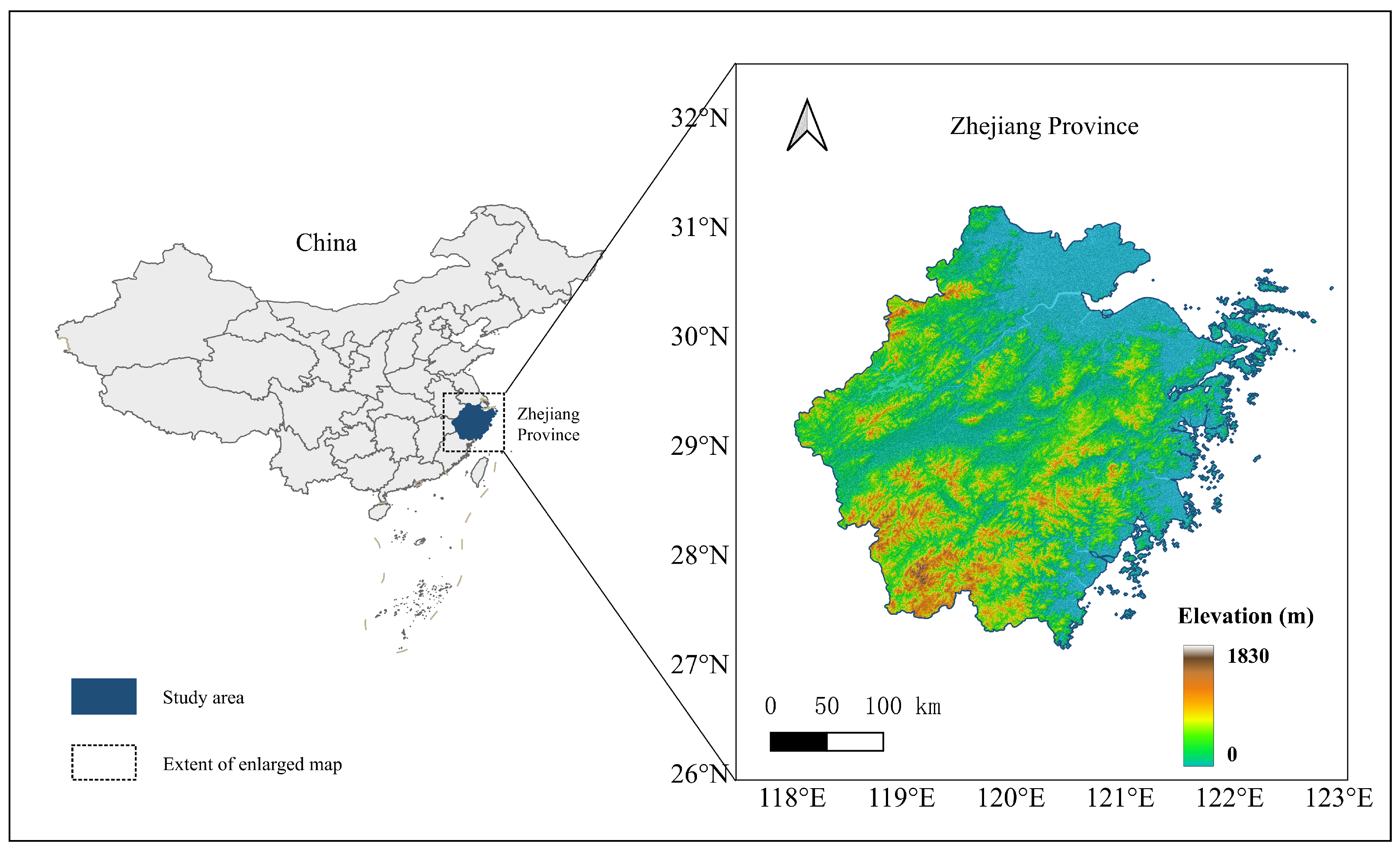
Figure 1. Geographical location and terrain elevation of the study area.
Remotesensing 18 03026 g001
Figure 2. Overall architecture of the proposed STAMP-GAN model.
Remotesensing 18 03026 g002
Figure 3. Structure of the STAMP-Net generator.
Remotesensing 18 03026 g003
Figure 4. Structure of the AM-ConvLSTM module.
Remotesensing 18 03026 g004
Figure 5. Architecture of the dual-branch temporal PatchGAN discriminator.
Remotesensing 18 03026 g005
Figure 6. Lead-time-resolved categorical metrics on the ERA5 dataset (0.5 mm h−1).
Remotesensing 18 03026 g006
Figure 7. Lead-time-resolved categorical metrics on the ERA5 dataset (5 mm h−1).
Remotesensing 18 03026 g007
Figure 8. Lead-time-resolved categorical metrics on the ERA5 dataset (10 mm h−1).
Remotesensing 18 03026 g008
Figure 9. Lead-time-resolved regression metrics on the ERA5 dataset. author:The redundant inset legend was removed, and the model names and data were checked and corrected to ensure consistency with the corresponding tables and the other lead-time-resolved figures.
Remotesensing 18 03026 g009
Figure 10. Lead-time-resolved categorical metrics on the CMA-S dataset at the 0.5 mm h−1 threshold.
Remotesensing 18 03026 g010
Figure 11. Lead-time-resolved categorical metrics on the CMA-S dataset at the 5 mm h−1 threshold.
Remotesensing 18 03026 g011
Figure 12. Lead-time-resolved categorical metrics on the CMA-S dataset at the 10 mm h−1 threshold.
Remotesensing 18 03026 g012
Figure 13. Lead-time-resolved categorical metrics on the CMA-S dataset at the 15 mm h−1 threshold.
Remotesensing 18 03026 g013
Figure 14. Lead-time-resolved categorical metrics on the CMA-S dataset at the 20 mm h−1 threshold.
Remotesensing 18 03026 g014
Figure 15. Lead-time-resolved regression metrics on the CMA-S dataset.
Remotesensing 18 03026 g015
Figure 16. Qualitative comparison of precipitation forecasts for an ERA5 test event initialized at 00:00 UTC on 27 May 2024 over Zhejiang Province. The first column shows the ERA5 reference precipitation fields, and the remaining columns show the corresponding forecasts generated by different models on the same 16 × 16 grid. T 1 T 6 denote forecast lead times of 1–6 h. All panels share the same precipitation color scale ranging from 0 to 200 mm h−1. The figure is used for qualitative comparison only and is not intended as an independent quantitative ranking of the models.
Remotesensing 18 03026 g016
Figure 17. Qualitative comparison of precipitation forecasts for an ERA5 test event initialized at 00:00 UTC on 19 September 2024 over Zhejiang Province. The first column shows the ERA5 reference precipitation fields, and the remaining columns show the corresponding forecasts generated by different models on the same 16 × 16 grid. T 1 T 6 denote forecast lead times of 1–6 h. All panels share the same precipitation color scale ranging from 0 to 200 mm h−1. The figure is used for qualitative comparison only and is not intended as an independent quantitative ranking of the models.
Remotesensing 18 03026 g017
Table 1. Summary of datasets and variables used in this study.
DatasetVariablePhysical MeaningTemporal ResolutionSpatial Resolution
ERA5tpTotal precipitation1 h0.25°
d2m2 m dewpoint temperature1 h0.25°
u10, v1010 m wind components1 h0.25°
mslMean sea-level pressure1 h0.25°
tccTotal cloud cover1 h0.25°
rh*Relative humidity1 h0.25°
DEMTerrain elevationStatic0.00028°
CMA-SPRE_1hHourly precipitation1 h0.05°
TEMAir temperature1 h0.05°
RHURelative humidity1 h0.05°
WIN_S_INSTWind speed1 h0.05°
WIN_D_INSTWind direction1 h0.05°
PRSAtmospheric pressure1 h0.05°
DPTDewpoint temperature1 h0.05°
DEMTerrain elevationStatic0.00028°
Note: rh* was derived from d2m and 2 m temperature (t2m) using the saturation vapor pressure relation; t2m was excluded from the model inputs because of its weak correlation with precipitation.
Table 2. Loss function components and corresponding weights.
Loss ComponentSymbolWeight
Weighted L1 regression L reg 1.0
Multi-threshold focal classification L cls 1.0
Occurrence-gate supervision λ m L mask 0.5
Global adversarial (WGAN-GP) λ adv L adv global 0.05
Last-3-frame adversarial (WGAN-GP) λ adv 3 L adv last 3 0.08
Temporal consistency λ t L temp 0.1
Spatial-gradient consistency λ s L grad 0.05
Table 3. Progressive component-ablation results for STAMP-GAN on the ERA5-based dataset using the revised two-dimensional DEM input strategy.
IndexConfigurationCSIPODFARMBEMAERMSECORRKGE
1Baseline0.59980.53590.3597−0.36600.47991.81650.48550.3804
2+STAMP-Net0.61930.84060.29840.06790.45021.14590.54310.3427
3+AM-ConvLSTM0.62320.84420.29610.04310.43651.28280.55580.4535
4+Dual-branch discriminator0.63330.86890.2560−0.02580.42741.05870.54490.4447
5+Hybrid loss0.63790.93500.24950.00260.38920.92600.61800.5866
Note: CSI, POD, and FAR are calculated at the 0.5 mm h−1 threshold and averaged over T1–T6. MBE, MAE, RMSE, CORR, and KGE are also averaged over T1–T6. Higher values indicate better performance for CSI, POD, CORR, and KGE; lower values indicate better performance for FAR, MAE, and RMSE; and MBE closer to zero is preferred. The table evaluates the progressive incorporation of the principal model components under the revised DEM strategy, where the two-dimensional DEM input is retained and the regional-mean DEM condition is removed from FiLM.
Table 4. Removal-based ablation results of the main components of STAMP-GAN.
ConfigurationCSIPODFARMBEMAERMSECORRKGE
Full STAMP-GAN0.63790.93500.24950.00260.38920.92600.61800.5866
w/o dual-branch discriminator0.62720.88500.27170.04680.42561.00300.60920.5290
w/o STAMP-Net0.61930.82760.2677−0.27480.37461.96490.54550.4638
w/o AM-ConvLSTM0.62730.84440.2878−0.01400.42681.02300.54480.5272
w/o hybrid loss0.61940.89070.33130.03940.43220.98850.56610.5362
Note: “w/o STAMP-Net” denotes replacing the proposed multi-scale generator with the baseline generator while retaining the remaining components. “w/o AM-ConvLSTM” removes the attention-modulated temporal evolution module. “w/o hybrid loss” removes the proposed hybrid loss configuration and uses the baseline loss setting. Higher values are better for CSI, POD, CORR, and KGE; lower values are better for FAR, MAE, and RMSE; and MBE closer to zero is preferred. Bold values indicate the best result for each metric.
Table 5. Multi-seed CSI comparison between the full STAMP-GAN and the variant without the last-three-frame discriminator. Values are reported as mean ± standard deviation over five paired runs.
Forecast RangeModelCSI at 0.5 mm h−1CSI at 5 mm h−1CSI at 10 mm h−1
T1–T6STAMP-GAN w/o D last 3 0.6294 ± 0.00520.2568 ± 0.00950.1304 ± 0.0062
T1–T6Full STAMP-GAN0.6343 ± 0.00400.2931 ± 0.00700.1455 ± 0.0084
T4–T6STAMP-GAN w/o D last 3 0.5777 ± 0.00560.1699 ± 0.00560.0383 ± 0.0059
T4–T6Full STAMP-GAN0.5811 ± 0.00680.1995 ± 0.00810.0604 ± 0.0067
Note: T1–T6 denotes the average over all six forecast lead times, whereas T4–T6 denotes the average over the final three forecast lead times. Values are reported as mean ± standard deviation over five paired random seeds. For T1–T6, the two-sided exact Wilcoxon signed-rank test yielded p = 0.4375 , p = 0.0625 , and p = 0.0625 at thresholds of 0.5, 5, and 10 mm h−1, respectively. For T4–T6, the full model achieved higher CSI for all five paired seeds at each threshold, with an exact two-sided Wilcoxon p-value of 0.0625 . The upward arrows (↑) indicate that higher CSI is better. Bold values indicate the higher CSI in each model comparison.
Table 6. Comparison of different DEM usage strategies.
ConfigurationCSIPODFARMBEMAERMSECORRKGE
Original DEM-conditioning configuration0.62670.92840.26950.04500.43310.99500.60210.5557
Revised model0.63790.93500.24950.00260.38920.92600.61800.5866
Revised model without DEM input0.61750.91770.25360.04500.40860.94960.59900.5726
Note: CSI, POD, and FAR are averaged over lead times T1–T6 at the 0.5 mm h−1 threshold. MBE, MAE, RMSE, CORR, and KGE are averaged over T1–T6. Higher values indicate better performance for CSI, POD, CORR, and KGE; lower values indicate better performance for FAR, MAE, and RMSE; and MBE closer to zero is preferred. Bold values indicate the best result for each metric.
Table 7. Threshold-based categorical verification results on the ERA5 dataset.
IndexModelsYearCSI ↑POD ↑FAR ↓
0.55100.55100.5510
1ConvLSTM20150.51330.23290.10750.86390.37570.13220.46020.58700.7651
2TrajGRU20170.54280.25090.11150.85640.34980.13580.41090.57240.7524
3U-Net++20180.55540.26070.10260.88740.37550.11860.40240.57380.7319
4PhyDNet20200.54460.27770.11400.91750.45740.22940.42980.60670.7404
5Swin Transformer20210.53460.27310.12270.92370.45490.17740.44230.61180.7728
6DGMR20210.59870.23140.09550.75770.30470.11090.33200.55630.7455
7MetNet3-R20230.53400.23520.10120.86880.30490.11370.42600.53210.7009
8PreDiff-R20230.39950.06030.00800.84740.38150.10590.56950.93400.9914
9SpateGAN20230.47810.26730.12010.86100.43090.16000.48010.60580.7217
10GraphCast-R20230.48970.26990.12280.91810.43340.21330.50230.67240.7824
11Diffusion Nowcasting20250.51360.19130.07010.77950.45020.20960.44510.76420.9103
12Fusion-202520250.48340.22620.09250.88120.30160.10580.49480.56940.7685
13STAMP-GAN (Ours)0.63790.29810.15510.93500.54030.36550.24950.52010.6990
Note: Bold values indicate the best performance, and underlined values indicate the second-best performance. The suffix “-R” denotes a regional adaptation of the corresponding architecture rather than a complete reproduction of the original system.
Table 8. Comparison of categorical and continuous verification metrics on the ERA5 dataset.
IndexModelsYearHSS ↑MAE ↓RMSE ↓MBE∼0Corr ↑
0.5510
1ConvLSTM20150.47430.36770.16980.54140.96770.12190.5819
2TrajGRU20170.53550.35670.18120.49330.95460.26860.5914
3U-Net++20180.43940.36680.16820.52221.01570.19240.5887
4PhyDNet20200.39970.38700.18610.47060.95670.04090.5871
5Swin Transformer20210.37170.38060.19460.41410.94670.11020.5783
6DGMR20210.55500.33100.15420.46100.92510.10540.5979
7MetNet3-R20230.53060.34040.16410.48490.95720.24890.5589
8PreDiff-R20230.06960.02130.00650.78011.66700.37940.4093
9SpateGAN20230.28210.37540.19540.51961.00470.12870.5793
10GraphCast-R20230.25200.37550.20170.64751.12800.38830.6009
11Diffusion Nowcasting20250.36750.25660.11640.50931.01260.18370.6033
12Fusion-202520250.53840.32390.15031.08352.17110.24140.6659
13STAMP-GAN (Ours)0.61580.40880.23860.38920.92600.00260.6180
Note: Bold values indicate the best performance, and underlined values indicate the second-best performance.
Table 9. Comparative results on the CMA-S dataset: threshold-based detection metrics (CSI and POD).
IndexModelsYearCSI ↑POD ↑
0.551015200.55101520
1ConvLSTM20150.40450.15460.05910.03430.01650.73760.30700.11570.06630.0311
2TrajGRU20170.40990.16690.08450.06290.04210.80570.51120.24760.18830.1258
3U-Net++20180.45110.20430.09960.07090.04110.80760.61460.34000.24970.1665
4PhyDNet20200.24550.18660.09450.07000.03630.86340.53370.23810.12620.0339
5Swin Transformer20210.18460.07660.03240.01190.00000.83060.42340.06300.02420.0000
6DGMR20210.40060.19520.09420.06180.02550.71590.42450.17990.09940.0306
7MetNet3-R20230.29250.16950.08450.05280.01850.79190.30150.12420.06510.0170
8PreDiff-R20230.33150.04630.00850.00400.00100.65850.14930.03000.01190.0023
9SpateGAN20230.32550.18850.08610.04420.02590.77550.58640.28190.13980.0305
10GraphCast-R20230.31230.14960.08570.05890.02190.81680.56130.24350.11470.0279
11Diffusion Nowcasting20250.11840.02580.00780.00520.00170.55610.35120.05390.01570.0024
12Fusion-202520250.43160.20450.08440.06590.03390.76030.47860.19050.12440.0685
13STAMP-GAN (Ours)0.49410.21340.10160.07150.04120.82520.69840.47140.37270.1948
Note: Bold values indicate the best performance, and underlined values indicate the second-best performance.
Table 10. Comparative results on the CMA-S dataset: threshold-based skill metrics (FAR and HSS).
IndexModelsYearFAR ↓HSS ↑
0.551015200.55101520
1ConvLSTM20150.53130.76810.88830.92750.96250.44490.22830.09990.06030.0303
2TrajGRU20170.54770.80570.89240.91810.94340.45950.24130.13830.10750.0750
3U-Net++20180.49410.78970.87230.89990.93000.51530.29420.16070.12180.0678
4PhyDNet20200.74510.81360.87510.89310.91210.16930.23130.15290.10920.0443
5Swin Transformer20210.81420.91600.96160.97711.00000.06130.13240.05070.00000.0000
6DGMR20210.60670.80470.86040.86840.88420.45220.28260.15530.10560.0468
7MetNet3-R20230.69140.79490.86970.88670.89540.29650.26770.13690.08930.0339
8PreDiff-R20230.59960.93680.98800.99380.99830.01070.01630.01020.00610.0016
9SpateGAN20230.65770.78570.84600.86040.88670.31490.26960.14440.07570.0478
10GraphCast-R20230.67060.83170.88760.89900.91060.26440.20200.13590.09620.0380
11Diffusion Nowcasting20250.82490.95490.98340.98700.99130.00610.00480.00650.00740.0030
12Fusion-202520250.50380.74310.87660.90010.89710.49420.30060.13340.11380.0602
13STAMP-GAN (Ours)0.33700.65750.80200.84100.87050.57760.30980.16830.12300.0714
Note: Bold values indicate the best performance, and underlined values indicate the second-best performance.
Table 11. Station-constrained sensitivity analysis of high-intensity precipitation detection on the CMA-S dataset.
ModelEvaluation DomainCSI@15POD@15FAR@15CSI@20POD@20FAR@20
U-Net++Full grid0.07090.24970.89990.04110.16650.9300
U-Net++Within 5 km0.08620.29030.89050.04610.16490.9254
STAMP-GANFull grid0.07150.37270.84110.04120.19480.8705
STAMP-GANWithin 5 km0.07340.37790.83850.04240.28980.8673
Note: “Within 5 km” denotes grid cells located within 5 km of at least one physical rain-gauge station, corresponding to 5179 of the 6400 grid cells. Metrics were calculated separately at each forecast lead time and subsequently averaged over T1–T6. Higher CSI and POD values and lower FAR values indicate better performance. Bold values indicate the best performance for each metric.
Table 12. Comparative results on the CMA-S dataset: continuous statistical metrics.
IndexModelsYearMAE ↓RMSE ↓MBE∼0Corr ↑
1ConvLSTM20151.27492.32770.92170.2844
2TrajGRU20171.20862.35930.86420.2914
3U-Net++20180.72521.87170.41340.3388
4PhyDNet20200.78231.88390.50580.3504
5Swin Transformer20211.65292.73921.34660.2206
6DGMR20210.50332.31670.12920.3426
7MetNet3-R20230.61381.67740.27230.3232
8PreDiff-R20231.15962.02890.49990.0303
9SpateGAN20230.98531.90340.71700.3378
10GraphCast-R20231.88232.84061.44390.0257
11Diffusion Nowcasting20251.12822.10490.65320.2954
12Fusion-202520250.90131.96210.60220.3337
13STAMP-GAN (Ours)0.38091.5205-0.04640.3743
Note: Bold values indicate the best performance, and underlined values indicate the second-best performance.
Table 13. Fractions Skill Score (FSS) on the ERA5 dataset at different precipitation thresholds and neighborhood sizes. Values are averaged over forecast lead times T1–T6.
Model0.5 mm h−15 mm h−110 mm h−1
1 × 1 3 × 3 5 × 5 1 × 1 3 × 3 5 × 5 1 × 1 3 × 3 5 × 5
ConvLSTM0.6970.8280.8640.3840.6150.7180.1810.3630.460
TrajGRU0.7030.8270.8640.3880.6020.6940.1830.3550.442
U-Net++0.7130.8400.8770.3990.6090.7010.1700.3170.384
PhyDNet0.7040.8070.8390.4230.6350.7280.2230.4190.521
Swin Transformer0.6610.7670.7960.2540.2990.3770.1610.2670.349
DGMR0.7480.8810.9220.3600.5700.6630.1560.2760.319
MetNet3-R0.6950.7960.8290.3690.5890.6850.1650.3050.357
PreDiff-R0.4290.6750.7220.4000.5050.5310.1670.3420.429
SpateGAN0.6470.7930.8260.4100.6380.7340.2000.3800.454
GraphCast-R0.5780.6120.6240.4220.6080.6770.1930.4030.516
Diffusion Nowcasting0.4410.6900.7360.3490.3570.3600.2000.3230.412
Fusion-20250.6510.7660.7970.3530.5690.6650.1520.2620.298
STAMP-GAN (Ours)0.7710.8960.9340.4390.6630.7590.2270.4240.527
Note: Bold values indicate the best performance, and underlined values indicate the second-best performance within each threshold–neighborhood combination. Higher FSS values indicate better spatial agreement.
Table 14. Fractions Skill Score (FSS) on the CMA-S dataset at different precipitation thresholds and neighborhood sizes. Values are averaged over forecast lead times T1–T6.
Model0.5 mm h−15 mm h−110 mm h−1
1 × 1 3 × 3 5 × 5 1 × 1 3 × 3 5 × 5 1 × 1 3 × 3 5 × 5
ConvLSTM0.3240.3990.4250.1920.3160.3770.1100.2410.313
TrajGRU0.3520.4210.4470.2050.3030.3440.1180.2260.268
U-Net++0.3830.5850.6260.2790.4200.4530.1500.2710.330
PhyDNet0.2700.3640.3910.2200.3000.3250.1120.2660.325
Swin Transformer0.1680.2180.2450.3080.3630.4170.2030.2460.317
DGMR0.4110.5470.6040.2730.4260.4450.1380.2660.325
MetNet3-R0.4290.5570.5940.2820.4180.4550.1590.2930.313
PreDiff-R0.2040.3860.4130.3110.3320.4420.2460.3170.423
SpateGAN0.3950.5040.5340.2630.3950.4530.1600.3250.406
GraphCast-R0.2340.2420.2450.1920.2380.2870.1330.1560.191
Diffusion Nowcasting0.2310.2730.2820.2820.2910.3140.1760.2200.288
Fusion-20250.3530.4220.4470.2570.4170.4430.1430.3330.334
STAMP-GAN (Ours)0.4880.5890.6610.3150.4290.4610.3410.3670.408
Note: Bold values indicate the best performance, and underlined values indicate the second-best performance within each threshold–neighborhood combination. Higher FSS values indicate better spatial agreement.
Table 15. Sliding-window counts and precipitation-event distributions for the training, validation, and testing splits.
DatasetSplitSliding WindowsTotal Target PixelsDryLightModerateHeavy
ERA5Training651110,000,8967,402,100 (74.0%)2,108,484 (21.1%)397,522 (4.0%)92,790 (0.9%)
ERA5Validation7201,105,920984,640 (89.0%)110,264 (10.0%)8610 (0.8%)2406 (0.2%)
ERA5Testing43816,729,2165,545,091 (82.4%)955,083 (14.2%)188,350 (2.8%)40,692 (0.6%)
CMA-STraining251496,537,60078,000,060 (80.8%)13,916,164 (14.4%)3,142,361 (3.3%)1,479,015 (1.5%)
CMA-SValidation70927,225,60025,510,728 (93.7%)1,375,212 (5.1%)231,255 (0.8%)108,405 (0.4%)
CMA-STesting4381168,230,400150,211,272 (89.3%)14,140,103 (8.4%)2,714,222 (1.6%)1,164,803 (0.7%)
Note: Each sliding-window sample contains six target precipitation frames. The total number of target pixels was calculated as the number of sliding windows multiplied by six forecast lead times and the number of grid cells per frame. Precipitation categories were calculated over all target pixels rather than sliding-window samples because each sample contains multiple forecast frames and spatial grid cells. Dry, light, moderate, and heavy precipitation were defined as p < 0.1 , 0.1 p < 2.5 , 2.5 p < 6 , and p 6 mm h−1, respectively. The dry–wet event-aware resampling strategy was applied only to the training set; the validation and test sets retained their original chronological distributions. Percentages may not sum to exactly 100% because of rounding.
Table 16. Multi-seed T1–T6 CSI comparison between the full STAMP-GAN and the variant without the last-three-frame discriminator.
SeedFull STAMP-GANSTAMP-GAN w/o D last 3
CSI@0.5 CSI@5 CSI@10 CSI@0.5 CSI@5 CSI@10
420.63790.29810.15520.62720.26950.1392
1230.63420.28110.14100.62800.26410.1308
20240.63140.29780.15300.63190.25170.1316
34070.62930.29460.14290.63680.24700.1220
56780.63860.29370.13520.62290.25180.1284
Mean ± std.0.6343 ± 0.00400.2931 ± 0.00700.1455 ± 0.00840.6294 ± 0.00520.2568 ± 0.00950.1304 ± 0.0062
Note: T1–T6 denotes the average over all six forecast lead times. CSI values are reported at precipitation thresholds of 0.5, 5, and 10 mm h−1. The two-sided exact Wilcoxon signed-rank test yielded p = 0.4375 , p = 0.0625 , and p = 0.0625 at thresholds of 0.5, 5, and 10 mm h−1, respectively. Bold values indicate the higher CSI in each model comparison.
Table 17. Multi-seed T4–T6 CSI comparison between the full STAMP-GAN and the variant without the last-three-frame discriminator.
SeedFull STAMP-GANSTAMP-GAN w/o D last 3
CSI@0.5 CSI@5 CSI@10 CSI@0.5 CSI@5 CSI@10
420.58650.20270.06180.58090.17390.0450
1230.58940.19480.05180.58500.16800.0369
20240.57920.21150.06530.57810.17520.0317
34070.57280.19810.06770.57150.17120.0440
56780.57760.19040.05540.57280.16120.0341
Mean ± std.0.5811 ± 0.00680.1995 ± 0.00810.0604 ± 0.00670.5777 ± 0.00560.1699 ± 0.00560.0383 ± 0.0059
Note: T4–T6 denotes the average over the final three forecast lead times. CSI values are reported at precipitation thresholds of 0.5, 5, and 10 mm h−1. The two-sided exact Wilcoxon signed-rank test yielded p = 0.0625 at all three precipitation thresholds. Bold values indicate the higher CSI in each model comparison.
Table 18. Normalized contingency-table counts for STAMP-GAN and Fusion-2025 on the CMA-S test set by precipitation threshold and forecast lead time.
ThresholdLeadObservedSTAMP TPSTAMP FPSTAMP FNFusion TPFusion FPFusion FN
10T1185,525120,823231,87364,702132,866480,43552,659
10T2185,572116,476262,06269,09670,451382,335115,121
10T3185,64493,741418,98191,90326,871178,107158,773
10T4185,72886,748578,75398,98011,60176,916174,127
10T5185,75179,552479,610106,199401039,065181,741
10T6185,67427,658307,631158,01677279185,597
15T197,32352,469109,30844,85464,650325,43732,673
15T297,35250,708173,69346,64422,773160,39174,579
15T397,39343,922270,03153,471495545,85392,438
15T497,44433,812286,86363,632103913,50996,405
15T597,45930,573281,07866,8869577097,364
15T697,445629299,08491,15311497,434
20T139,46013,38829,69826,07219,980158,06319,480
20T239,47310,95350,07728,520252029,75136,953
20T339,49610,508107,28128,988213631139,283
20T439,517592461,53233,593010939,517
20T539,524472855,87234,7960039,524
20T639,52165119,68638,8700039,521
Note: Observed denotes the number of observed event samples, defined as grid–time points for which the observed precipitation was greater than or equal to the specified threshold. TP, FP, and FN denote hits, false alarms, and misses, respectively.
Disclaimer/Publisher’s Note: The statements, opinions and data contained in all publications are solely those of the individual author(s) and contributor(s) and not of MDPI and/or the editor(s). MDPI and/or the editor(s) disclaim responsibility for any injury to people or property resulting from any ideas, methods, instructions or products referred to in the content.