Article

Homogeneous Terrain Unit Extraction by Integrating Superpixel Segmentation and Multiscale Region Merging: A Case Study in the Deeply Incised Valleys of Southeastern Tibet

1
College of Water Resources and Hydropower, Sichuan University, Chengdu 610065, China
2
Power China Chengdu Engineering Corporation Limited, Chengdu 610072, China
*
Author to whom correspondence should be addressed.
Remote Sens. 2026, 18(17), 3028; https://doi.org/10.3390/rs18173028
Submission received: 29 June 2026 / Revised: 22 August 2026 / Accepted: 31 August 2026 / Published: 4 September 2026

Highlights

What are the main findings?
  • SSM-HTU uses slope units as local statistical references while allowing final HTUs to cross slope-unit boundaries where terrain morphology remains continuous.
  • Compared with MSS, SSM-HTU improves reference-object coverage, spatial overlap, and boundary correspondence with a small Precision trade-off, while maintaining broadly comparable performance across contrasting geomorphological zones.
What are the implications of the main findings?
  • Separating hillslope-scale statistical context from final geometric constraints provides a practical way to represent local within-slope terrain heterogeneity in deeply incised valleys.
  • Mapping-unit support affects factor-specific spatial associations, indicating that spatial support, attribute aggregation, and scale should be considered explicitly in downstream statistical interpretation.

Abstract

Mapping mountain surfaces requires spatial units that represent both hillslope-scale structure and local within-slope terrain heterogeneity. Hydrological slope units provide limited representation of within-slope objects, whereas general object-based segmentation is sensitive to fragmentation and scale selection. We developed a homogeneous terrain unit extraction framework based on superpixel segmentation and multiscale region merging (SSM-HTU), in which initial slope units serve as local statistical references and within-slope terrain objects are generated through slope-unit-conditioned morphometric representation, superpixel initialization, distribution-sensitive region merging, and a nested partition hierarchy. The framework was applied to the 5136 km2 Yuqu River Basin in southeastern Tibet. Of 971 expert-interpreted reference HTUs, 680 were reserved for independent geometric evaluation; 1329 historical landslides were additionally used for supplementary spatial association analysis across mapping-unit schemes. Relative to the eCognition Multiresolution Segmentation (MSS) baseline, SSM-HTU showed a slight decrease in Precision from 0.8432 to 0.8340, while Recall (directional reference-object coverage) increased from 0.7615 to 0.8011, area-weighted IoU from 0.6710 to 0.6945, and Boundary F1 at a 12.5 m tolerance from 0.5980 to 0.6810, indicating greater reference-object coverage, spatial overlap, and boundary correspondence without uniform improvement across all geometric metrics. Across four geomorphological zones, area-weighted IoU ranged from 0.671 to 0.724 and Boundary F1 from 0.651 to 0.709, with non-monotonic regional variation. Mapping-unit schemes also yielded factor-dependent spatially stratified associations, underscoring the importance of spatial support in downstream statistical analysis. SSM-HTU therefore provides an object-based mapping framework for representing local within-slope terrain heterogeneity within a hillslope-scale statistical context in deeply incised valleys.

1. Introduction

Mountain surfaces vary continuously in space, whereas quantitative analysis generally requires their discretization into mapping units with explicit spatial extents to aggregate terrain and environmental attributes and represent unit-scale spatial relationships [1,2]. Terrain analysis and digital geomorphological mapping commonly describe such surfaces using terrain units, landform elements, or terrain objects [3,4], with emphasis on within-unit similarity, between-unit differentiation, and spatial connectivity [1,5]. The boundaries and internal composition of these objects are inherently scale dependent [6,7] and vary with the target feature, selected terrain attributes, and DEM spatial resolution [7,8]. In this study, a homogeneous terrain unit (HTU) is operationally defined as a spatially connected surface object delineated at a given DEM resolution and analysis scale, within which selected DEM-derived attributes are relatively consistent and distinguishable from those of adjacent units. Homogeneity is therefore relative to the selected attributes and scale rather than absolute.
Mountain mapping units can be broadly grouped into three categories according to their spatial support and boundary-generation mechanisms. Regular grids provide standardized spatial support for DEMs, remote-sensing products, and regional statistical analyses, facilitating attribute calculation, spatial matching, and cross-regional comparison [1,9]. Their boundaries, however, are determined by the sampling structure rather than terrain discontinuities, and changes in cell size can alter the representation of terrain attributes and spatial patterns [1,7]. Slope units provide a more terrain-oriented representation by organizing the surface into hillslope objects according to ridge–valley or divide–drainage relationships, with a relatively coherent hydrological–topological structure [9,10]. They are widely used in mountain environmental and landslide studies [9,11], but their internal homogeneity depends on the delineation method, parameterization, analysis scale, and terrain setting [10,11]. Individual slope units may therefore still contain local platforms, slope breaks, or contrasting slope forms, motivating local subdivision, region merging, and multiscale refinement [10,12]. A third category derives objects directly from terrain attributes. Object-based or homogeneous-surface segmentation groups pixels with similar geomorphometric, textural, and spatial-neighborhood characteristics into connected objects, allowing local within-slope terrain elements to be represented more explicitly [2,13]. These objects, however, remain sensitive to the target feature, input variables, DEM resolution, segmentation scale, and parameterization and may become fragmented or scale mismatched where terrain transitions are gradual, boundaries are weak, or objects of different scales coexist [13,14].
These three representations are therefore complementary rather than interchangeable: regular grids emphasize standardized spatial support, slope units emphasize hillslope-scale hydrological–topological organization, and attribute-driven objects emphasize local within-slope terrain heterogeneity [1,9]. Recent studies have sought to combine hillslope structure with local object information through slope-unit optimization, boundary or knowledge constraints, multiscale segmentation, graph-based representations, and region merging [10,15]. Hybrid segmentation and local-optimization approaches provide an important methodological basis for such integration [16,17]. The unresolved issue is how these different forms of spatial information should be organized during object generation. The hillslope-scale terrain context should inform local feature representation without being imposed as a non-crossable final boundary, while objects at different granularities should remain linked through a traceable nested partition hierarchy. This issue is especially relevant in deeply incised mountain valleys, where long hillslopes contain terraces, local platforms, slope breaks, and steep-to-gentle transitions; strong ridge–valley boundaries coexist with gradual slope-form transitions, and terrain objects occur at multiple nested scales [6,18]. An effective framework therefore needs to retain hillslope-scale context while allowing local terrain continuity and multiscale object relationships to shape the final partition.
To address this need, we developed a homogeneous terrain unit extraction framework based on superpixel segmentation and multiscale region merging (SSM-HTU). Initial slope units serve as local statistical references rather than final boundary constraints, while slope-unit-conditioned morphometric representation, superpixel initialization, distribution-sensitive region merging, and a nested partition hierarchy are integrated to delineate within-slope terrain objects without imposing the initial slope-unit boundaries on the final partition. Using the Yuqu River Basin in southeastern Tibet as a case study, we address three questions: (1) whether SSM-HTU can delineate HTUs with reasonable geometric correspondence to expert-interpreted terrain objects; (2) how a unified representative level performs across different geomorphological zones; and (3) how spatially stratified associations between environmental factors and unit-level landslide occurrence differ among mapping-unit schemes. This study thus provides an object-based mapping framework for jointly representing hillslope-scale terrain contexts and local within-slope terrain heterogeneity in deeply incised valleys.

2. Study Area and Data

2.1. Study Area

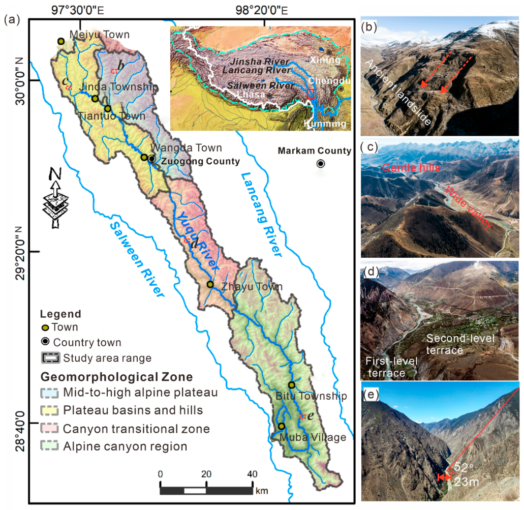
The study area covers the Yuqu River Basin in southeastern Tibet, extending southeastward from Meiyu Township to the confluence of the Yuqu and Nujiang rivers and lying predominantly within Zogang County, Chamdo City, Tibet Autonomous Region. The basin spans 97°30′–98°30′E and 28°00′–30°30′N, covers approximately 5136 km2, and extends about 335 km along the main valley, with a transverse width of approximately 10–45 km. The main stem of the Yuqu River generally trends northwest–southeast. Elevation ranges from approximately 2000 m in the valley to more than 5400 m along adjacent divides, producing pronounced local relief and a landscape characterized by deeply incised valleys, long hillslopes, and strong topographic variation.
Based on relief, valley morphology, and hillslope structure, the study area was divided into four geomorphological zones: plateau wide-valley, plateau mountainous, transitional gorge, and alpine gorge. The plateau wide-valley zone is characterized by broad, gentle valleys, intermontane basins, and platforms or terraces, whereas the plateau mountainous zone has greater relief and more continuous hillslopes. The transitional and alpine gorge zones exhibit progressively deeper valley incision, with terraces and slope breaks becoming prominent in the former and deeply incised V-shaped valleys, long steep slopes, and large relative relief in the latter [10]. Figure 1a shows the spatial distribution of the four zones, and Figure 1b–e present representative landscapes. The zoning was used only to describe geomorphological variations and evaluate regional performance and did not contribute to SSM-HTU boundary generation.

2.2. Topographic and Ancillary Data

Terrain analysis used the DEM distributed with the ALOS PALSAR high-resolution radiometric terrain-corrected product (ALOS_PSR_RTC_HIGH, Version 1) by the NASA Alaska Satellite Facility Distributed Active Archive Center (ASF DAAC). The DEM is derived from SRTM GL1, with an original pixel spacing of approximately 30 m and elevations referenced to the EGM96 orthometric datum. During RTC processing, ASF converted the elevations to ellipsoidal heights and resampled the DEM to 12.5 m. Accordingly, 12.5 m denotes the working-grid spacing used in this study rather than the native spatial scale of the source elevation information, which remains approximately 30 m. After mosaicking, clipping, and masking invalid data, the DEM was projected to WGS 84/UTM Zone 47N (EPSG:32647).
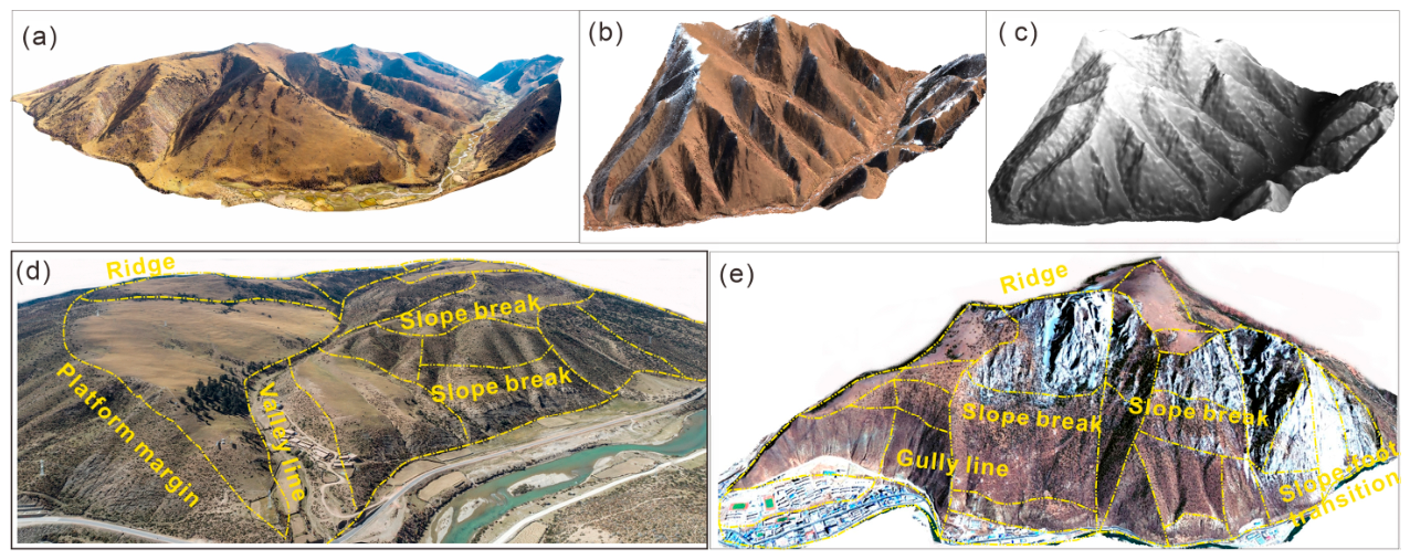
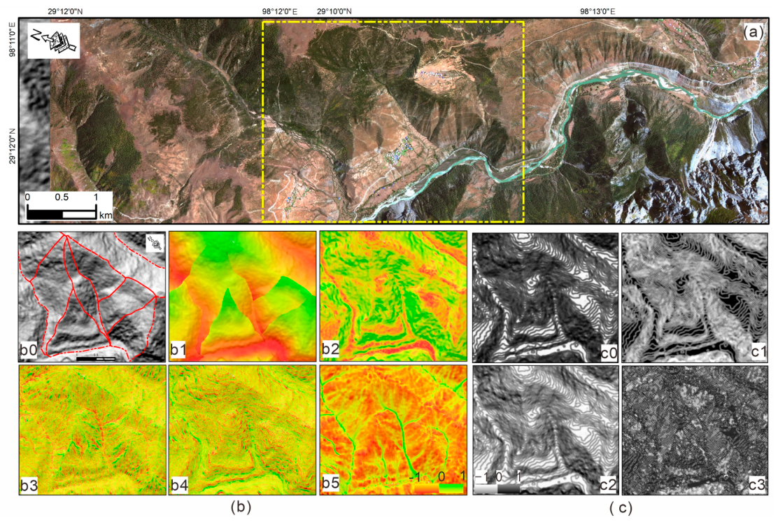
Initial slope units were generated from the same working DEM using r.slopeunits v1.0 [9] to construct the slope-unit-conditioned morphometric features; parameter settings are provided in Section 3. Ancillary data included 1 m Gaofen-2 imagery acquired on 20 January 2020 and UAV orthophotos covering part of the study area [10]. Where available, these data were used to verify platform and terrace margins, local slope breaks, and the continuity of relatively weak DEM-derived boundaries (Figure 2a–c).
The historical landslide inventory comprised 1329 landslides compiled from visual interpretation of three-dimensional Google Earth imagery, field-verification records, and landslide inventories for the Nujiang region compiled by Yang and Zhang [19]. Landslide areas were mainly 0.005–0.60 km2, with nearly 90% of the areas being smaller than 0.25 km2 [19]. The historical landslide inventory was used for the supplementary comparative spatial association analysis in Section 5; its observed area-scale distribution was also considered when defining the study-specific 5000 m2 minimum-area post-processing threshold.

2.3. Expert-Interpreted Reference Terrain Units

An expert-interpreted HTU dataset was established to evaluate the geometric agreement of automated partitions with identifiable terrain objects and their boundaries. A reference HTU was defined as a spatially connected object with a closed boundary and relatively consistent dominant terrain morphology. Boundaries were delineated primarily from consistently identifiable ridges, valleys, slope breaks, platform or terrace margins, steep-to-gentle transitions, and convex-to-concave slope-form transitions [6]. Interpretation combined three-dimensional DEM visualization, multidirectional hill-shading, topographic profiles, slope, and curvature. Gaofen-2 and available UAV imagery were used to verify local boundaries and their continuity. Detailed operational criteria for reference-HTU interpretation, retention, and low-confidence exclusion are provided in Supplementary Section S1.1 and Supplementary Table S2. Representative examples of these boundary-recognition criteria are illustrated in Figure 2d,e.
Two doctoral researchers with relevant disciplinary expertise independently interpreted the same areas using a common set of rules and then cross-checked the delineations object by object. Disagreements were jointly reviewed using topographic profiles, DEM-derived representations, and ancillary imagery. Only objects with reproducibly locatable boundaries, unambiguous topology, and consistent subdivision decisions were retained; objects with diffuse boundaries or unresolved interpretations were excluded.
Reference HTUs were delineated independently of the initial slope-unit boundaries and were allowed to cross them where terrain morphology remained continuous. The reference dataset was finalized before spatial overlay with the initial slope units and was not subsequently modified. In total, 971 high-confidence reference HTUs were retained for geometric evaluation; these objects intersected 332 initial slope units. In SSM-HTU, the initial slope units were used only for local feature conditioning and did not determine reference-HTU boundaries or subdivision levels.

3. Methodology: The SSM-HTU Model

3.1. Overview of the SSM-HTU Framework

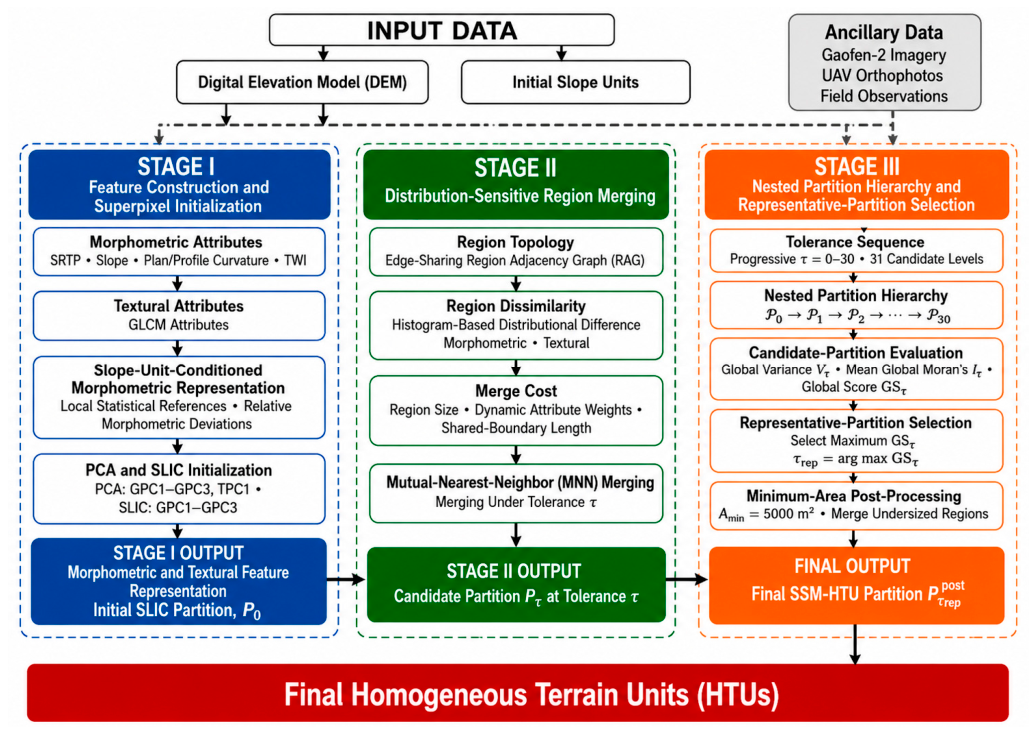
SSM-HTU uses the 12.5 m working-grid DEM and its derived morphometric and textural attributes to delineate spatially connected terrain units that are relatively homogeneous internally and distinguishable from adjacent regions. The workflow comprises five main stages: feature construction, initial-object generation, distribution-sensitive region merging, representative-partition selection, and minimum-area post-processing. First, DEM-derived morphometric attributes are converted to a slope-unit-conditioned morphometric representation; the morphometric and textural branches are then processed separately by principal component analysis (PCA) to construct their respective feature representations. SLIC is then used to generate spatially connected initial objects. These objects are progressively merged on a region adjacency graph (RAG) using a distribution-sensitive merge cost, producing a nested partition hierarchy as the merging tolerance increases. A representative partition is subsequently selected by jointly evaluating within-unit feature dispersion and spatial association among adjacent regions, after which minimum-area post-processing yields the final HTUs. Here, “multiscale” refers specifically to the nested partition hierarchy generated through progressive region merging. Figure 3 summarizes the input data, major processing stages, and corresponding outputs of SSM-HTU.

3.2. Terrain Attributes and Slope-Unit-Conditioned Morphometric Representation

3.2.1. Morphometric and Textural Attributes

The morphometric branch includes slope-unit relative topographic position (SRTP), slope, plan curvature, profile curvature, and the topographic wetness index (TWI). For pixel i within slope unit u , SRTP is defined as:
SRTP i = z i z u min z u max z u min
where z i is the elevation of pixel (i), and z u m i n and z u m a x are the minimum and maximum elevations within slope unit u , respectively. When z u m i n = z u m a x , SRTP is set to 0. SRTP ranges from 0 to 1 and represents the relative elevation position of a pixel within the corresponding slope unit.
Slope, plan curvature, and profile curvature were calculated from the projected working DEM. Slope was derived using the Horn 3 × 3 finite-difference operator, whereas plan and profile curvature were calculated using the Zevenbergen–Thorne 3 × 3 method [20,21]. For near-horizontal pixels, both curvature measures were set to 0 when the local gradient was below a predefined numerical-stability threshold, thereby avoiding numerical anomalies caused by very small denominators. Flow accumulation for TWI was calculated using the multiple-flow-direction algorithm implemented in GRASS GIS r.watershed and converted to specific catchment area a i [22,23]:
TWI i = ln a i tan max { β i , β min }
where β i is the local slope angle and β min = 0.01 is used for near-horizontal pixels. TWI was calculated only where the DEM, slope, and flow-accumulation values were all valid.
The textural branch characterizes local elevation arrangements in the working DEM using gray-level co-occurrence matrices (GLCMs). The DEM was first linearly quantized into 32 gray levels using fixed elevation bounds for the entire study area. GLCMs were then calculated within a 7 × 7-pixel moving window at a displacement of one pixel in four directions: 0°, 45°, 90°, and 135°. After symmetrization and probability normalization, angular second moment, entropy, contrast, correlation, and inverse difference moment were calculated for each direction and averaged across the four directions, yielding five textural attribute channels [24]. Figure 4 shows the initial slope units and the spatial distributions of the principal morphometric and textural attributes.

3.2.2. Slope-Unit-Conditioned Morphometric Representation

Initial slope units were generated from the same working DEM and its hydrological terrain information using r.slopeunits v1.0 [9]. The minimum circular variance of aspect was set to 0.3 and the threshold-reduction factor to 11. The initial flow-area threshold, minimum slope-unit area, and cleanup-area threshold were 1.0 × 10 6 , 3.0 × 10 5 , and 1.5 × 10 4 m2, respectively, yielding 6514 initial slope units.
Because SRTP already represents the relative elevation position of each pixel within its slope unit, as defined in Equation (1), it was not subjected to additional conditioning. Slope, plan curvature, profile curvature, and TWI were transformed into local deviations relative to the statistical background of their respective slope units:
x i , t c = x i , t μ u , t x u , t max x u , t min , i u
where x i , t is the morphometric attribute t at pixel i , and μ u , t , x u , t min , and x u , t max are the mean, minimum, and maximum of that attribute within slope unit u , respectively. When the within-unit range is zero, the conditioned value is set to 0. This slope-unit-conditioned normalization centers each attribute on its within-unit mean and scales it by the within-unit range, thereby representing positive and negative deviations from the local hillslope statistical background.
After conditioning, the results from individual slope units were mosaicked into continuous feature channels covering the common valid area. The initial slope units serve only as local statistical references: neither their identifiers nor their geometric boundaries enter the subsequent SLIC distance calculation, RAG adjacency definition, or merge-cost calculation. Consequently, SLIC initial objects and final HTUs may cross initial slope-unit boundaries where the criteria based on feature similarity and spatial adjacency are satisfied.

3.2.3. PCA Feature Representation

Morphometric and textural attributes were independently z -standardized within the common valid area of each branch and subjected to separate principal component analyses (PCA) [25]. The morphometric branch comprised SRTP together with the slope-unit-conditioned slope, plan curvature, profile curvature, and TWI, whereas the textural branch comprised the five GLCM attributes. For each branch, principal components were retained until the cumulative explained variance reached at least 90%, reducing redundancy among the input attributes while preserving separate morphometric and textural feature representations.
The retained components were then z -standardized again to place them on comparable numerical scales. The retained morphometric components were used for SLIC initial-object generation, whereas the retained components from both branches were used for region representation, distribution-sensitive region merging, and candidate-partition evaluation. The number of retained components in each branch and the corresponding explained variances are reported in Section 4.1.

3.3. Initial Object Generation by SLIC

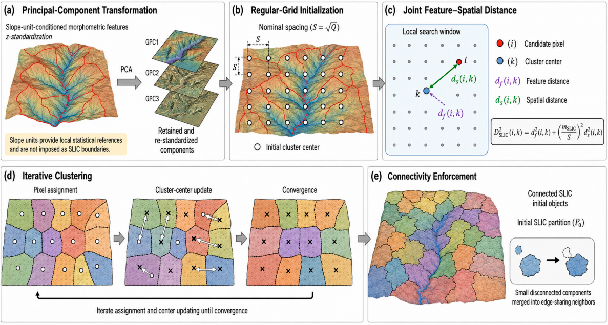
Simple linear iterative clustering (SLIC) was used to partition the standardized morphometric principal component feature field into spatially connected initial terrain objects [26]. The feature and spatial distances between pixel i and cluster center k are defined as
d f 2 i , k = c = 1 3 g i , c μ k , c 2 , d s 2 i , k = x i x k 2 + y i y k 2
and the combined SLIC distance is
D SLIC 2 i , k = d f 2 i , k + m SLIC S 2 d s 2 i , k
where g i , c and μ k , c are the feature values at pixel (i) and cluster center (k), respectively, for the (c)-th morphometric principal component; m SLIC is the compactness parameter; and S is the nominal cluster-center spacing. Larger m SLIC values increase the contribution of spatial proximity and favor more compact and regular objects, whereas smaller values increase sensitivity to local feature differences.
The target mean superpixel size Q was defined as the nominal number of valid pixels per requested initial object. For a calibration window containing Nvalid valid pixels, the requested cluster number K, target mean size Q, and nominal cluster-center spacing S satisfy
Q = N valid K , S = Q , K full = round N valid Q
Equation (5) provides an explicit link between the requested cluster number and the nominal granularity of the initial objects. Based on superpixel sizes on the order of 102 pixels considered in previous SLIC evaluations [26] and the need to balance terrain-boundary preservation against initial-object granularity, the target mean superpixel size Q was examined over a study-specific range of approximately 120–180 valid pixels. One 700 × 700-pixel calibration window was selected from each of the four geomorphological zones to represent different valley forms and hillslope structures. Within each window, K ∈ {2800,3200,3600,4000} was evaluated, corresponding to nominal mean sizes of approximately 175.0, 153.1, 136.1, and 122.5 valid pixels per superpixel, respectively.
The SLIC parameters were calibrated sequentially according to their distinct roles in initial-object generation. Because K directly controls the requested number and nominal granularity of the initial superpixels, it was evaluated first while m SLIC was held constant. Consistent with the compactness–regularity trade-off inherent in SLIC [26], a moderate compactness value around 20 has been used in remote-sensing applications to obtain compact and spatially regular initial regions [27]. Using this literature-supported moderate compactness level as a reference, m SLIC ∈ {18,20,22,24} was defined as a narrow study-specific candidate set for subsequent compactness refinement. For the initial K-sensitivity analysis, m SLIC = 22 was adopted as an interior reference value within this range. It remains close to the literature-supported value of 20 while placing slightly greater weight on spatial regularity during the comparison of different K settings. After the first-stage K calibration, the selected K was held fixed, and the full candidate set m SLIC ∈ {18,20,22,24} was evaluated to refine the trade-off between local boundary adherence and spatial regularity. All candidate settings were evaluated against the same calibration reference data using Boundary Recall, Under-segmentation Error, achieved mean superpixel area after connectivity enforcement, and the spatial continuity and regularity of the initial objects.
For each parameter setting, SLIC was initialized using the nominal center spacing S and updated through local search and iterative clustering. Additional details on the search extent, iterative updating, convergence criterion, and connectivity enforcement are provided in Supplementary Section S1.2. After iteration, connectivity was checked using a four-neighbor rule. Non-main connected components smaller than 0.25Q were merged into the raster-edge-sharing neighboring object with the smallest distance between mean morphometric principal component values. The selected parameter settings were applied uniformly across the study area without geomorphology-specific retuning, and the resulting connected superpixels constituted the initial SLIC partition (P0) for subsequent region merging. The overall SLIC initial-object generation procedure, from feature preparation and regular-grid initialization to iterative clustering and connectivity enforcement, is summarized in Figure 5.

3.4. Distribution-Sensitive Region Merging

3.4.1. Region Representation and Merge Cost

A region adjacency graph (RAG) was constructed from the SLIC initial partition P 0 [16]. Each object was represented by a graph node, and adjacency was defined only between regions sharing horizontal or vertical raster edges; corner-only contact was excluded. Initial slope-unit boundaries were not used to filter adjacency. Each active region stored its pixel count n a and histograms of the retained morphometric and textural principal components; for each adjacent region pair (a) and (b), the number of shared raster edges l a b was also recorded. The retained morphometric and textural principal component sets are denoted by M and T , with d M = M and d T = T .
For each retained and re-standardized principal component, B = 256 fixed equal-width histogram bins were defined from the range of valid pixel values across the full study area. The bin boundaries remained unchanged throughout region merging. Let p a , c , h and p b , c , h denote the probability histograms of regions a and b , respectively, for feature channel c , where h indexes the histogram bin. Their mean distribution is
r a b , c , h = p a , c , h + p b , c , h 2
Based on the Jensen—Shannon divergence, the distributional difference between regions a and b in channel c is defined as [28]
D ab , c = 2 h = 1 B p a , c , h ln p a , c , h r ab , c , h + 2 h = 1 B p b , c , h ln p b , c , h r ab , c , h
where terms with zero probability are treated as 0. Equation (6) uses natural logarithms and is numerically equal to four times the standard Jensen—Shannon divergence. Distributional differences for the morphometric and textural branches are aggregated as
D ab M = 1 d M c = 1 3 D ab , c , D ab T = 1 d T D ab , 4
To dynamically adjust the relative contributions of morphometric and textural information according to the local morphometric distributions, the morphometric peak concentration of region a is defined as
κ a = 1 d M c = 1 3 max h   p a , c , h
For adjacent regions a and b , the morphometric and textural weights are
ω ab M = min κ a , κ b , ω ab T = 1 ω ab M
and the combined attribute difference is
H ab = ω ab M D ab M + ω ab T D ab T
When the morphometric distributions of both regions are strongly concentrated, morphometric differences receive greater weight. If either region has a more dispersed morphometric distribution, the relative contribution of textural information increases. Because regional histograms change as merging proceeds, the peak concentrations and corresponding weights are updated dynamically.
The merge cost combines region size, the combined distributional difference, and shared-boundary length:
C ab = n a n b n a + n b H ab l ab γ , γ = 0.5
The region-size term affects the merging order of regions of different sizes, whereas the shared-boundary term assigns lower costs, all else being equal, to regions with greater boundary contact. The exponent γ = 0.5 gives shared-boundary length a sublinear influence on the merge cost. C a b is calculated only for adjacent regions sharing a boundary in the RAG.

3.4.2. RAG-Based Mutual Nearest Neighbor Merging

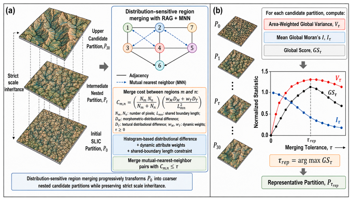
Within the current RAG, each active region first identifies the adjacent region with the minimum merge cost. Adjacent regions a and b form an admissible mutual nearest neighbor (MNN) merge pair only when each is the other’s minimum-cost neighbor and their merge cost does not exceed the current tolerance τ :
b = argmin j N a C aj , a = argmin i N b C bi   C ab τ
where N a and N b denote the current adjacency sets of regions a and b , respectively. The MNN condition restricts local competition among candidate merges and prevents the same region from participating in multiple merges during a single candidate search.
After each merge, the pixel count, feature histograms, adjacency relationships, and shared-edge counts of the merged region are updated, followed by recalculation of the weights and merge costs. The partition at the current τ is output once no adjacent pair satisfies Equation (9). Tied candidates and adjacency conflicts are resolved in a fixed deterministic order, as detailed in Supplementary Section S1.3. The tolerance τ is then increased stepwise, with each new level initialized from the preceding partition, thereby generating the nested partition hierarchy described in Section 3.5.

3.5. Nested Partition Hierarchy and Representative-Partition Selection

Let the SLIC initial partition be P 0 . Progressive merging was performed over the tolerance range τ = 0–30 in unit increments, producing 31 candidate levels. For any τ > 0 , merging started from the preceding partition P τ 1 and its RAG and proceeded according to Section 3.4 until no mutually minimum-cost adjacent pair remained whose merge cost did not exceed the current tolerance, yielding P τ .
Because the procedure permits only complete-region merges and does not allow region splitting or boundary recovery, adjacent candidate levels satisfy
R P τ , R = Q Q R Q , Q R P τ 1
Thus, every region at a coarser level consists entirely of regions from the preceding level, forming a fine-to-coarse nested partition hierarchy. The upper tolerance was set to τ = 30 , at which the number of regions remained greater than the 6514 initial slope units, thereby retaining within-slope subdivision.
Within-unit feature dispersion for each candidate partition was evaluated using area-weighted Global Variance [29]. Let P τ contain M τ regions, with n a pixels in region a . All retained principal components form the feature set C = M T , where M and T denote the retained morphometric and textural component sets, respectively, and d = d M + d T is the total number of feature channels. If σ a , c 2 denotes the population variance of feature channel c within region a , then
V τ = 1 d N a = 1 M τ n a c C σ a , c 2 , N = a = 1 M τ n a
Lower V τ indicates lower within-partition feature dispersion.
Spatial association among the mean feature values of adjacent regions was characterized using Global Moran’s I . For feature channel c , let x a , c denote the mean feature value of region a , x τ , c the corresponding mean across all regions at the current candidate level, and z a , c = x a , c x τ , c . The binary adjacency weight is w a b = 1 when regions a and b share a raster edge and w a b = 0 otherwise. Using a symmetric binary adjacency matrix without row standardization,
I τ , c = M τ W τ a b w a b z a , c z b , c a z a , c 2
W τ = a b w a b , I τ = 1 4 c = 1 4 I τ , c
Lower I τ indicates a weaker positive spatial association among the mean feature values of adjacent regions.
To jointly characterize within-unit feature dispersion and spatial association among adjacent regions, V τ and I τ were reverse min–max normalized over the fixed set of 31 candidate levels:
V ~ τ = V max V τ V max V min , I ~ τ = I max I τ I max I min G S τ = V ~ τ + I ~ τ
The tolerance corresponding to the representative partition is defined as
τ rep = argmax τ { 0 , , 30 } G S τ
If multiple candidate levels attain the same maximum score, the smaller τ is selected to retain the relatively finer partition. The resulting representative partition P τ rep is then passed to the independent minimum-area post-processing stage. The distribution-sensitive region-merging procedure, nested partition hierarchy, and representative-partition selection are summarized in Figure 6.

3.6. Minimum-Area Post-Processing

After selection of the representative partition P τ rep , minimum-area post-processing was to merge local regions that were too small to be retained as independent mapping objects. Considering the size distribution of historical landslides in the study area, the minimum mapping-unit threshold was set to A min = 5000 m2, corresponding to 32 working-grid pixels at 12.5 m spacing.
Regions were processed in ascending order of area. For any region smaller than A min , the merge target was selected only from neighboring regions sharing raster edges, with priority given to the neighbor with the smallest current merge cost C a b . If multiple neighbors had the same minimum cost, the region sharing the longer boundary was selected. Each operation merged complete regions and simultaneously updated the merged region’s area and feature histograms, together with the corresponding RAG adjacency relationships. Processing continued until all regions had areas of at least A min . The final post-processed partition is denoted by P τ rep post . The computational environment, stage-wise runtime, measured peak memory usage, and principal scaling characteristics of the basin-scale SSM-HTU workflow are reported in Supplementary Section S1.9 and Table S6.

3.7. Accuracy Assessment, Baselines, and Ablation Configurations

The 971 high-confidence reference HTUs described in Section 2.3 were used to evaluate object overlap and boundary agreement. To prevent information reuse between SLIC parameter calibration and final evaluation, any reference HTU used to evaluate candidate SLIC parameter settings in any of the four calibration windows was assigned in its entirety to the calibration subset; objects crossing window boundaries were not clipped. Consequently, 291 reference HTUs were used exclusively for SLIC parameter selection, whereas the remaining 680 constituted an independent test set for overall evaluation, geomorphological zone evaluation, and framework comparison.
Let A i denote an automatically delineated unit and R j a reference HTU. For each automatic unit, the unique reference object with the maximum IoU was selected in the automatic-unit-to-reference direction:
j i = argmax j A i R j A i R j
Multiple automatic units were allowed to match the same reference HTU. Based on this best-match relationship, Precision, Recall, and IoU for automatic unit A i are defined as [30]
P i = A i R j i A i , R i = A i R j i R j i J i = IoU i = A i R j i A i R j i
Here, P i is the proportion of the automatic unit contained within its best-matching reference object, R i is the proportion of that reference object covered by the automatic unit, and J i measures their spatial overlap. Overall Precision, Recall, and IoU were calculated using automatic-unit area weights:
w i = A i k = 1 N A A k , X aw = i = 1 N A w i X i , X { P , R , J }
The mean unweighted IoU was also calculated as
IoU ¯ unw = 1 N A i = 1 N A J i
to characterize average overlap across automatic units of different sizes and limit the influence of large units that receive greater weight in area-weighted statistics.
Boundary agreement was evaluated using deduplicated automatic and reference boundary networks, denoted as B A and B R , respectively. Shared boundaries redundantly represented by adjacent units were retained only once, while line segments coinciding with the outer study area boundary or internal NoData boundaries were excluded. The boundary-matching tolerance was set to one working-grid pixel, d = 12.5 m. This distance is used only as the tolerance for Boundary F1 evaluation and does not represent either the native spatial resolution of the source DEM or the positional accuracy of the final boundaries. Let L denote boundary length. Boundary Precision and Boundary Recall are defined as [31]
B P d = L B A Buffer B R , d L B A , B R d = L B R Buffer B A , d L B R
and Boundary F1 is
B F 1 d = 2 B P d B R d B P d + B R d
The same object-matching and boundary-evaluation rules were used for the overall assessment and the four geomorphological-zone assessments. Reference HTUs crossing geomorphological-zone boundaries were assigned to the zone with which they had the largest area of overlap. Automatic units best matched to those reference HTUs were then included in the corresponding zone-specific evaluation.
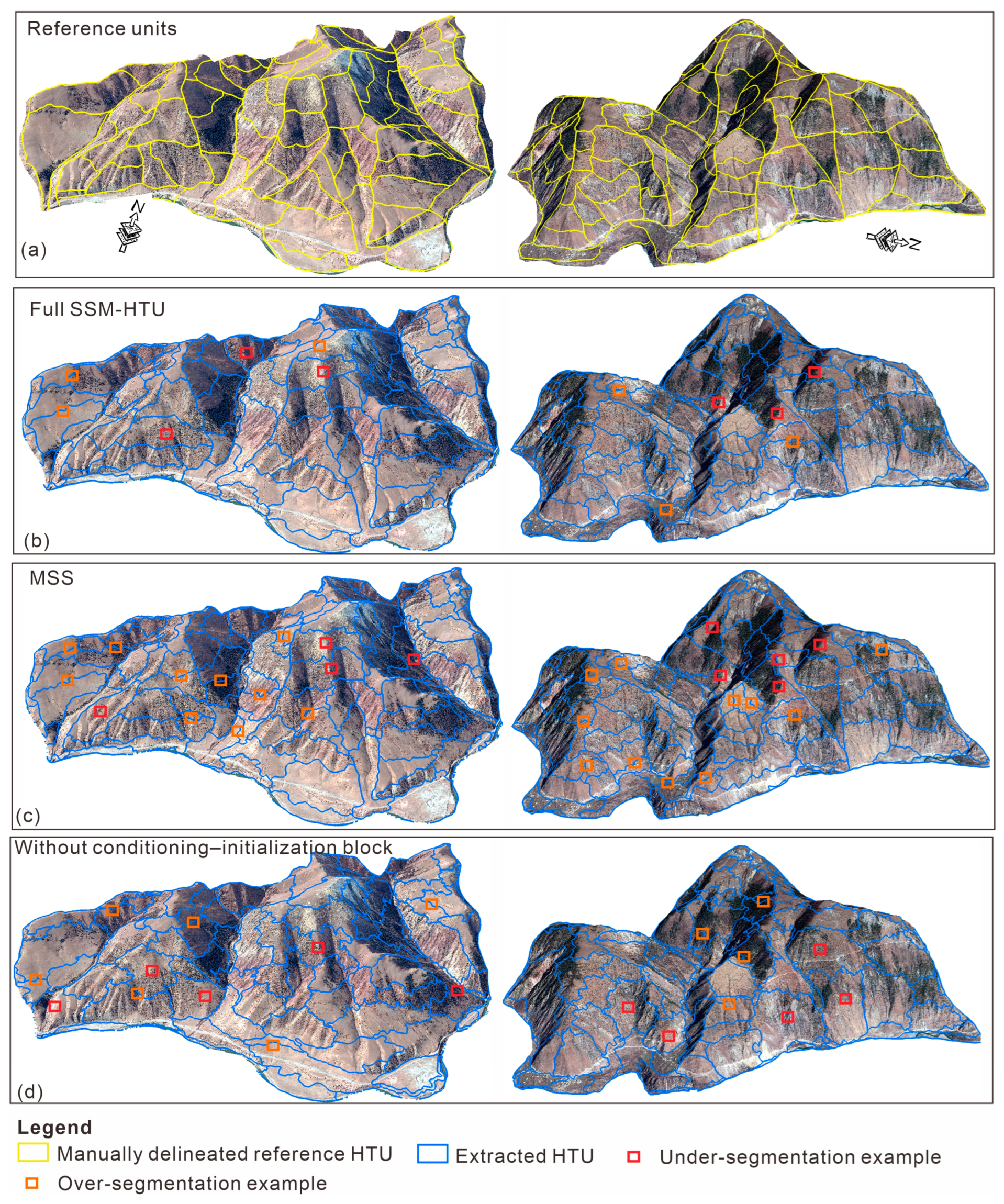
The MSS baseline, Full SSM-HTU, the Without conditioning–initialization configuration, and Mean-based SSM-HTU were compared using the same working DEM, common valid area, 680 independent test HTUs, 5000 m2 post-processing rule, and evaluation protocol. The comparison was designed to maintain broadly comparable overall partition granularity across configurations while avoiding configuration-specific retuning, except where required for the external MSS baseline. The MSS baseline used Multiresolution Segmentation in eCognition Developer 9.0 to generate terrain objects directly from pixels [32]. Input features were equally weighted; shape and compactness were set to 0.5 and 0.8, respectively; and the scale parameter was adjusted so that the resulting partition granularity was approximately comparable to that of Full SSM-HTU. Additional implementation and comparability settings for the MSS baseline are provided in Supplementary Section S1.4 and Supplementary Table S3.
Full SSM-HTU used the complete framework. Mean-based SSM-HTU replaced only the distributional differences in Equations (6) and (7) with differences between regional means while retaining all other procedures and parameter settings unchanged; its resulting partition granularity therefore remained close to that of Full SSM-HTU without additional scale retuning. The Without conditioning–initialization configuration jointly removed slope-unit conditioning and SLIC initialization while retaining the subsequent region-merging procedure, minimum-area post-processing rule, and evaluation settings. No separate tuning was introduced to force its final unit count to match Full SSM-HTU; the resulting partition remained broadly comparable in overall granularity but was somewhat finer. This configuration was therefore used to evaluate the conditioning–initialization block only at the combined module level.

4. Results

4.1. Feature Representation and SLIC Parameter Selection

Using a cumulative explained variance threshold of ≥90%, three principal components were retained for the morphometric branch. GPC1, GPC2, and GPC3 explained 51%, 25%, and 14% of the variance, respectively, whereas TPC1 alone explained 91% of the variance in the textural branch (Table 1).
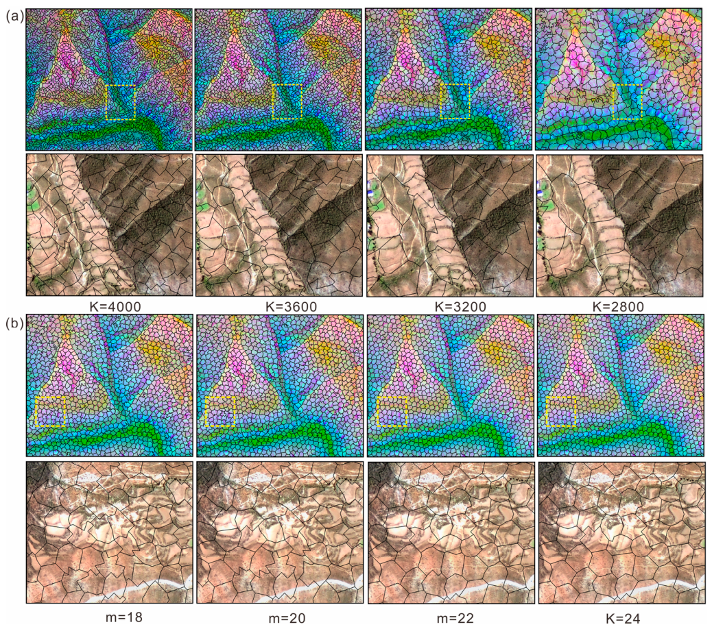
In the first calibration stage, with mSLIC = 22 fixed as the reference compactness setting defined in Section 3.3, the candidate K settings showed broadly consistent responses across the four 700 × 700-pixel calibration windows. Increasing K generally increased Boundary Recall and reduced Under-segmentation Error while producing progressively finer initial objects (Table 2). Spatially, smaller K values produced larger objects that more often spanned local slope breaks and terrain transitions, whereas larger values generated denser boundaries and a greater number of small superpixels (Figure 7a). The improvement in boundary metrics was most pronounced when K increased from 2800 to 3200, whereas further increases to 3600 and 4000 yielded progressively smaller gains while continuing to reduce initial-object size. Accordingly, K = 3200 was adopted as a compromise between boundary correspondence and limiting unnecessarily fine initial fragmentation rather than as the setting that maximized any single metric. This setting corresponded to a nominal mean superpixel size of Q = 153.1 valid pixels. Applied to approximately 3.287 × 10⁷ valid pixels across the study area, this target mean initial-object size corresponded to approximately 2.15 × 10⁵ requested clusters.
After K = 3200 had been selected in the first calibration stage, mSLIC was further evaluated at this fixed K. Across the tested values, increasing mSLIC from 18 to 24 slightly reduced Boundary Recall and increased Under-segmentation Error, while the mean superpixel area remained close to 24,000 m2 (Table 3). Smaller mSLIC values produced more irregular objects that followed local feature variations more closely, whereas larger values produced more regular objects but showed lower boundary correspondence at some terrace margins and slope transitions (Figure 7b). Although mSLIC = 18 and 20 gave slightly better Boundary Recall and Under-segmentation Error, mSLIC = 22 produced more spatially regular initial objects while retaining boundary performance close to the lower-compactness settings; increasing the value further to 24 resulted in a clearer reduction in boundary correspondence. Accordingly, mSLIC = 22 was retained as the final balanced setting between local boundary sensitivity and spatial regularity.
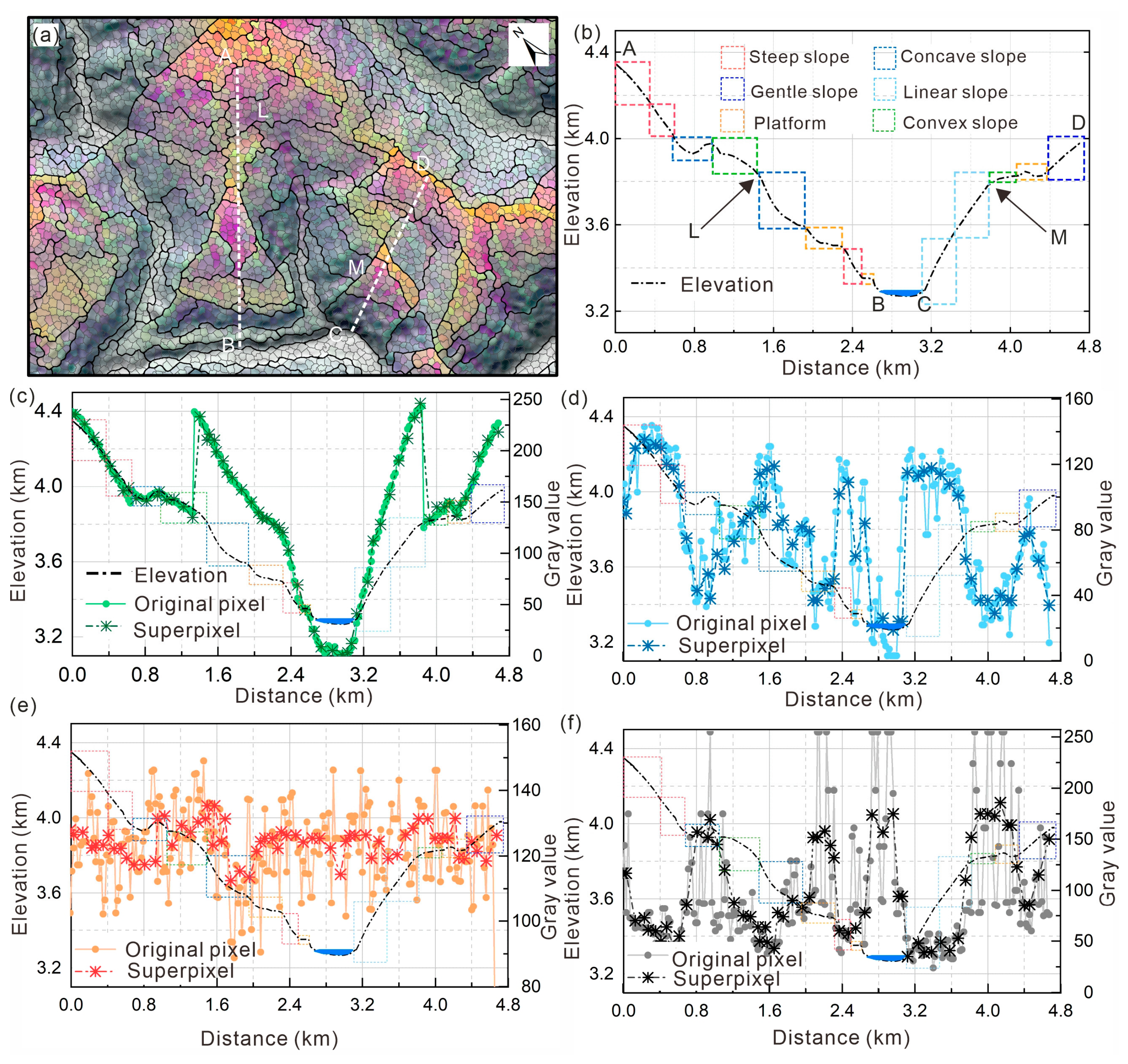
Figure 8 illustrates the pixel-to-object transformation of the retained feature components along a representative cross-valley transect. Aggregation within SLIC initial objects reduced short-range pixel fluctuations, while broader terrain trends and several transition locations remained identifiable in the illustrated transect between terrain segments. GPC1 retained a relatively continuous ridge-to-valley-floor trend, GPC2 showed clearer changes at several steep-to-gentle and slope-form transitions, and GPC3 preserved subtler local differences. Pixel-level fluctuations in TPC1 were also reduced after object aggregation while several transition locations remained identifiable. The SLIC initial objects thus formed spatially continuous feature representations for subsequent distribution-sensitive region merging.

4.2. Hierarchical Evolution and Representative-Partition Selection

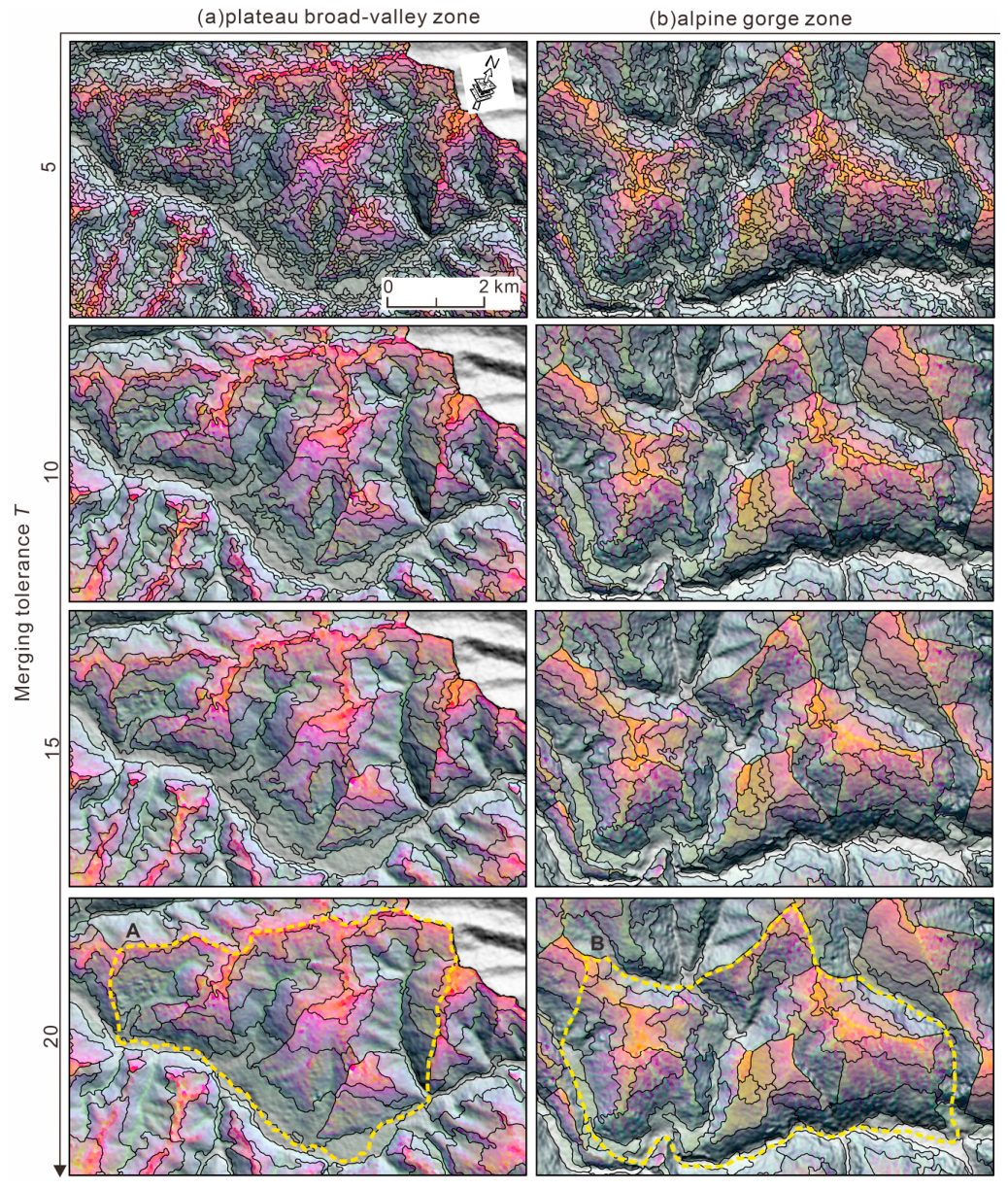
Across the predefined tolerance sequence τ = 0–30, the candidate partitions progressively coarsened as τ increased. The representative areas in Figure 9 illustrate this nested evolution. At τ = 5, the partition still retained relatively fine internal boundaries and numerous small terrain objects. By τ = 15, many of these smaller adjacent objects had been integrated, producing more spatially continuous regions while several major terrain transitions remained distinguishable. Further coarsening at τ = 20 incorporated some still-identifiable neighboring terrain elements into the same regions. These examples show how increasing τ progressively suppresses finer internal boundaries while preserving the nested parent–child relationship among candidate partitions.
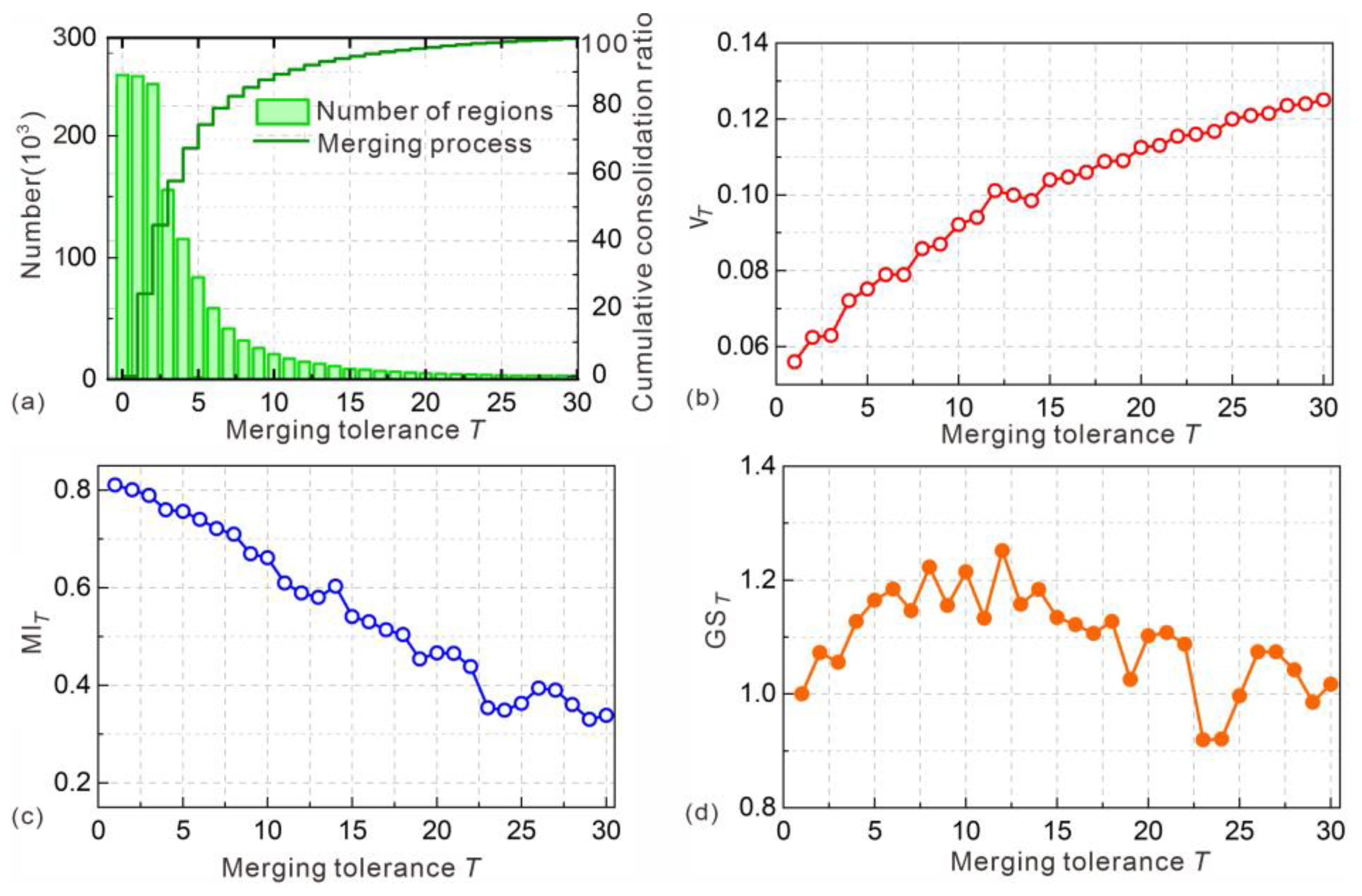
At the basin scale, the region number decreased continuously with increasing τ, whereas the cumulative merging proportion increased rapidly at lower tolerances and then gradually leveled off (Figure 10a). Area-weighted Global Variance Vτ generally increased as the partitions became coarser, whereas the mean Global Moran’s Iτ generally decreased with local fluctuations (Figure 10b,c). The Global Score GSτ increased initially and then declined, reaching its maximum at τ = 12 within the predefined candidate sequence (Figure 10d). Accordingly, τ = 12 was selected as the basin-wide representative level and P12 as the representative partition. Before minimum-area post-processing, P12 contained 37,207 regions; application of the 5000 m2 minimum-area rule reduced the number to 37,114, yielding the final partition P12post.
Figure 9. Representative nested evolution of SSM-HTU partitions at τ = 5, 10, 15, and 20 in two geomorphological settings: (a) plateau wide-valley zone; and (b) alpine gorge zone. Yellow dashed outlines indicate representative terrain domains used for visual comparison. Region A denotes the local extent presented in Figure 11, whereas region B denotes the local extent presented in Figure 12.
Remotesensing 18 03028 g009
Figure 10. Hierarchical evolution and representative-partition selection across the predefined tolerance sequence τ = 0–30: (a) region number and cumulative merging proportion; (b) area-weighted Global Variance Vτ; (c) mean Global Moran’s Iτ; and (d) Global Score GSτ, which reached its maximum at τ = 12.
Remotesensing 18 03028 g010

4.3. Spatial Characteristics and Terrain-Zone Evaluation of the Final HTUs

The final partition contained 37,114 HTUs, with an overall median area of 0.1743 km2. Across the four geomorphological zones, the median HTU area ranged from 0.1627 to 0.1885 km2, with substantial overlap among the zone-specific distributions. Based on the 680 independent test HTUs, the overall area-weighted IoU and Boundary F1 were 0.6945 and 0.6810, respectively. Zone-specific performance varied non-monotonically, with area-weighted IoU ranging from 0.671 to 0.724 and Boundary F1 from 0.651 to 0.709 (Table 4). These results indicate that the basin-wide representative level maintained broadly comparable geometric agreement across all four geomorphological zones, supporting its use for unified basin-scale mapping despite moderate regional variations in performance.
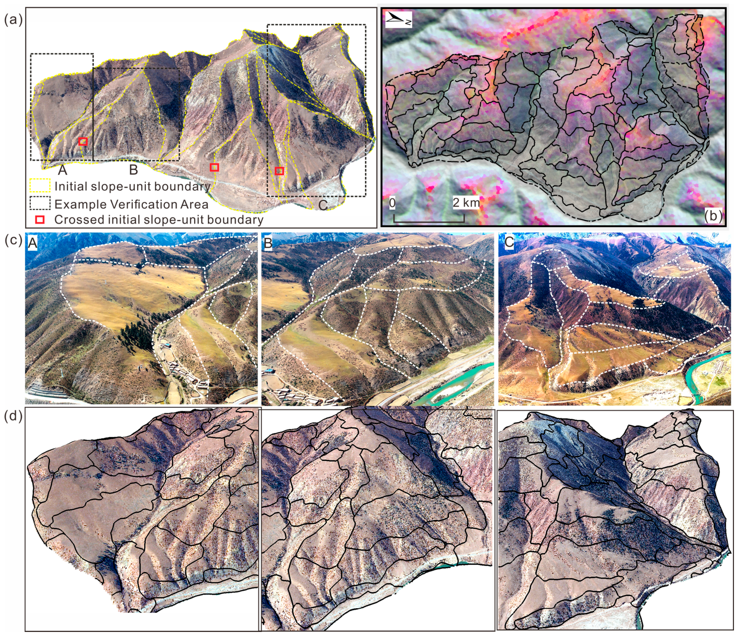
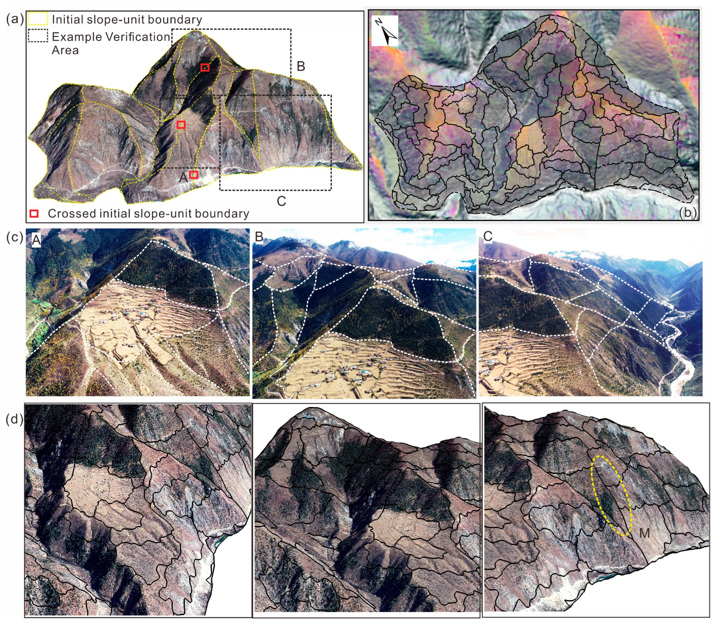
Figure 11 and Figure 12 illustrate the spatial characteristics of the final partition in the plateau wide-valley and alpine gorge zones. In the plateau wide-valley zone, extracted boundaries mainly followed broad gentle ridges, hillslope subdivisions, and slope foot-to-valley floor transitions. In the alpine gorge zone, they were more commonly aligned with distinct ridges, steep valley slopes, steep-to-gentle transitions, and local platform margins. Local discrepancies occurred mainly along gradual or weak terrain transitions in the plateau wide-valley zone and around smaller or geometrically complex objects in the alpine gorge zone.
Figure 11. Qualitative geomorphological assessment of the final SSM-HTU partition in the plateau wide-valley zone: (a) three-dimensional terrain view and representative subareas A–C; (b) plan-view HTU boundaries; (c) field and oblique-view photographs with interpreted terrain discontinuities; and (d) final HTU boundaries overlaid on optical imagery. In panel (a), A–C denote the locations of the three representative local example areas shown from left to right in panels (c,d).
Remotesensing 18 03028 g011
Figure 12. Qualitative geomorphological assessment of the final SSM-HTU partition in the alpine gorge zone: (a) three-dimensional terrain view; (b) plan-view HTU boundaries; (c) field and oblique-view photographs with interpreted ridgelines, terrace margins, and slope transitions; and (d) final HTU boundaries overlaid on optical imagery. In panel (a), A–C denote the locations of the three representative local example areas shown from left to right in panels (c,d). The yellow dashed ellipse in panel (d) highlights a representative local discrepancy, labeled M.
Remotesensing 18 03028 g012
Some final HTUs crossed initial slope-unit boundaries where terrain morphology remained continuous, without introducing new divisions along those boundaries (red boxes in Figure 11a and Figure 12a). These representative cross-boundary cases were broadly consistent with the continuous terrain objects identified by expert interpretation and with the framework design in which initial slope-unit boundaries were not imposed as final partition constraints.

4.4. Framework-Level Comparison and Targeted Ablation Analysis

The MSS baseline, Full SSM-HTU, and the two targeted ablation configurations were evaluated using the same 680 independent test HTUs, object-matching rules, and geometric metrics (Table 5). The four configurations produced broadly comparable overall partition granularity, although the Without conditioning–initialization configuration yielded a somewhat finer partition. MSS contained 36,583 units with a median area of 0.1830 km2, compared with 37,114 units and 0.1743 km2 for Full SSM-HTU. Mean-based SSM-HTU remained particularly close to the full framework, with 37,463 units and a median area of 0.1708 km2, whereas the Without conditioning–initialization configuration produced 38,351 units with a smaller median area of 0.1569 km2. As described in Section 3.7, no additional scale retuning was applied to the two internal ablation configurations.
Relative to the MSS baseline, Full SSM-HTU showed a slight decrease in Precision, whereas Recall, area-weighted IoU, mean unweighted IoU, and Boundary F1 increased. The two largest changes were in area-weighted IoU, from 0.6710 to 0.6945, and Boundary F1, from 0.5980 to 0.6810. Thus, the full framework did not improve all geometric metrics simultaneously; greater reference-object coverage, spatial overlap, and boundary correspondence were accompanied by a small loss in Precision.
Joint removal of the conditioning–initialization block reduced Recall, both IoU measures, and Boundary F1 relative to Full SSM-HTU and resulted in a somewhat finer partition. Mean-based SSM-HTU retained partition granularity close to that of the full framework and achieved a slightly higher Precision but a lower Recall, both IoU measures, and Boundary F1. Under the current experimental configuration, the distribution-sensitive representation was therefore associated with greater reference-object coverage, spatial overlap, and boundary correspondence than the mean-based alternative. The departures in the major geometric metrics were larger for the joint-removal configuration than for the mean-based replacement; however, because the joint-removal configuration also produced a somewhat finer partition, these differences are interpreted only at the combined-module level rather than as isolated effects of slope-unit conditioning or SLIC initialization.
The spatial comparisons in Figure 13 were consistent with these quantitative patterns. Within the illustrated areas, the MSS baseline and the configuration without the conditioning–initialization block showed more local subdivisions along some otherwise continuous hillslopes, whereas Full SSM-HTU produced more spatially continuous objects in these examples. These local patterns do not imply a uniformly finer basin-wide MSS partition. All configurations nevertheless exhibited local boundary displacement or partition differences near weak terrain transitions and geometrically complex boundaries.

5. Comparative Spatial Association Analysis Using Different Mapping Units

5.1. Analytical Design and Mapping-Unit Support

To examine how spatially stratified associations between environmental factors and landslide occurrence vary among mapping-unit schemes, Geodetector analysis was conducted using three spatial supports: a 30 m regular grid (GRID), locally optimized multiscale slope units (LMSO-SU) [10], and SSM-HTU. The analysis included 1329 historical landslides and 20 conditioning factors. It was designed as a supplementary downstream spatial association analysis, independent of the geometric evaluation, and was not used to assess the geometric accuracy of SSM-HTU. The candidate conditioning-factor library and screening status are summarized in Supplementary Section S1.5 and Supplementary Table S1.
For each mapping scheme, a unit was assigned Y = 1 when landslide coverage exceeded 1% of its area and Y = 0 otherwise [33]. All positive and negative units were retained without balancing or downsampling. The resulting sample sizes, mean unit areas, and positive-unit prevalence differed substantially among the three spatial supports (Table 6).
Conditioning factors were represented according to the spatial support of each mapping scheme. For GRID, values were extracted directly from the spatially aligned factor grids. For LMSO-SU and SSM-HTU, continuous factors were represented by the arithmetic mean of valid pixels within each unit, whereas categorical factors were assigned according to the class occupying the largest proportion of the unit area. Detailed rules for mapping-unit response assignment, NoData handling, and factor aggregation are provided in Supplementary Section S1.6.

5.2. Geodetector Configuration and Interpretation

Continuous factors were discretized separately for each mapping scheme. For each factor–mapping scheme combination, five discretization methods—equal interval, natural breaks, quantile, geometric interval, and standard deviation—were evaluated using 5–10 strata, yielding 30 candidate configurations. The configuration with the highest factor-detector q-value was selected and then fixed for subsequent factor, interaction, and risk detection [34]. Categorical factors retained their original classes.
Accordingly, cross-scheme differences cannot be attributed solely to mapping-unit geometry or area. They reflect the combined effects of spatial support, within-unit attribute aggregation, and scheme-specific discretization on the resulting spatially stratified associations.
The factor detector quantifies the correspondence between factor stratification and the spatial differentiation of unit-level landslide occurrence [35]:
q = 1 h = 1 L N h σ h 2 N σ 2
where L is the number of strata, Nh and σh2 are the number of mapping units and the variance of the landslide response within stratum h, respectively, and N and σ2 are the total number of units and the overall response variance. The theoretical range of q is 0–1, with higher values indicating stronger spatial statistical correspondence between factor stratification and the distribution of landslide-positive units.
The interaction detector compares the jointly stratified q(X1 ∩ X2) with the corresponding single-factor q-values to classify relationships such as bivariate enhancement, nonlinear enhancement, and independence [35]. The interaction classification criteria used in this study are provided in Supplementary Section S1.6.
The risk detector compares mean landslide responses among strata of the same factor [35]. Because Y is binary, the mean response within a stratum is equivalent to the proportion of landslide-positive units in that stratum. Pairwise differences among valid strata were evaluated using two-sided Welch’s t-tests [36] with an unadjusted threshold of p < 0.05. No additional multiple-comparison correction was applied. For the cross-scheme summary, a factor was counted when at least one pairwise contrast satisfied this criterion. Detailed risk-detector procedures and the resulting candidate high-prevalence intervals or categories are provided in Supplementary Section S1.7 and Supplementary Table S4.

5.3. Cross-Scheme Spatial-Association Results

The three mapping-unit schemes produced distinct spatial-association patterns under their respective spatial supports, aggregation procedures, and discretization configurations (Table 7). Overall, both polygon-based schemes showed higher summary single-factor and interaction q-values than GRID. The mean single-factor q was 0.04 for GRID, compared with 0.14 for SSM-HTU and 0.13 for LMSO-SU, while the corresponding maximum interaction q-values were 0.22, 0.69, and 0.67, respectively. GRID had no factor with q > 0.1 and no interaction with q > 0.6, whereas both polygon-based schemes contained multiple factors and interactions above these descriptive thresholds.
Differences between the two polygon-based schemes were comparatively small and depended on the summary measure. SSM-HTU had a slightly higher mean single-factor q and maximum interaction q, and nine interaction pairs exceeded q = 0.6, compared with six for LMSO-SU. In contrast, LMSO-SU contained 16 factors with at least one qualifying unadjusted pairwise contrast at p < 0.05, compared with 12 for SSM-HTU (Table 7). These contrasts indicate that the two polygon-based spatial supports did not exhibit a uniform ordering across association measures.
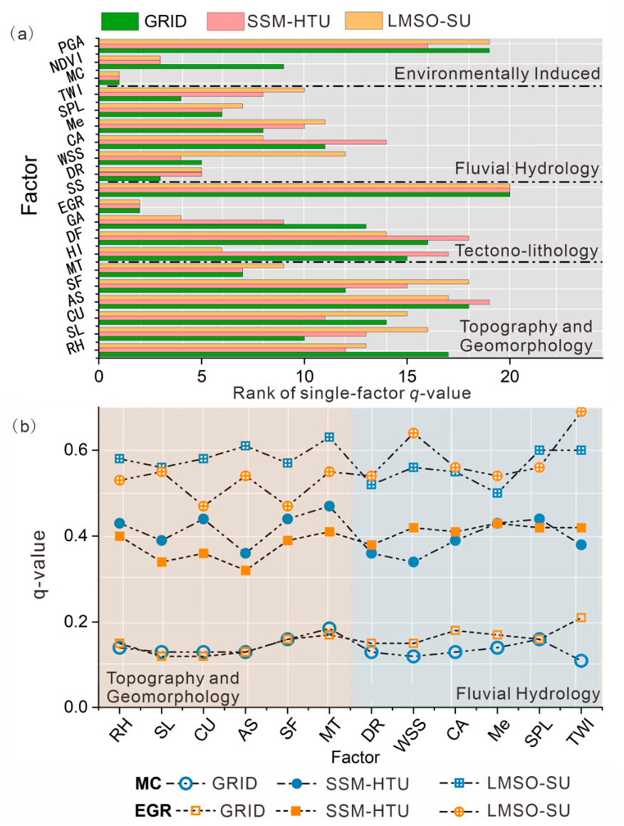
Single-factor rankings likewise varied among mapping schemes (Figure 14a). EGR ranked relatively high under all three schemes, whereas MC ranked high under both polygon-based schemes but lower under GRID. PGA and SS generally occupied lower-ranking positions. Several intermediate factors, including CU, AS, MT, HI, DF, WSS, and CA, changed position more noticeably across schemes, indicating that mapping-unit selection affected not only the overall magnitude of spatial association but also the relative ordering of factor-specific associations.
Representative interaction results showed a similar pattern (Figure 14b). For the illustrated combinations of MC and EGR with selected topographic–geomorphological and fluvial–hydrological factors, joint q-values were generally lower under GRID and higher under the two polygon-based schemes. Several illustrated LMSO-SU combinations reached or exceeded q = 0.6; across the complete interaction set, however, SSM-HTU contained more high-value interactions (nine versus six), with maximum interaction q-values of 0.69 and 0.67 for SSM-HTU and LMSO-SU, respectively. The threshold q > 0.6 is used only as a descriptive criterion for summarizing comparatively high interaction values and does not represent a criterion for statistical significance.

5.4. Sensitivity Analysis After Excluding Delineation-Related Factors

To examine the extent to which the cross-scheme comparison was influenced by factors directly involved in SSM-HTU delineation, slope (SL), curvature (CU), and the topographic wetness index (TWI) were excluded from the original 20-factor single-factor results, and the remaining 17 factors were re-summarized. AS was retained because, although DEM-derived, it was not directly used in SSM-HTU delineation. No discretization or Geodetector calculation was repeated; the analysis therefore represents a subset comparison based on the original scheme-specific stratifications and q-values.
After exclusion, GRID retained a mean q of 0.040, whereas the corresponding values for LMSO-SU and SSM-HTU were 0.131 and 0.112. Median q-values were 0.039, 0.123, and 0.103, respectively, and the numbers of factors with q > 0.1 were 0, 10, and 9. Thus, the two polygon-based schemes continued to show higher summary association statistics than GRID, but their relative ordering changed: within the 17-factor subset, both the mean and median q were higher for LMSO-SU than for SSM-HTU.
Factor-level results further showed that the highest q-values for individual factors occurred under different mapping schemes; complete factor-level results for the 17-factor sensitivity analysis are provided in Supplementary Section S1.8 and Supplementary Table S5. The two polygon-based schemes therefore exhibited factor-dependent spatial-association patterns rather than a consistent ordering across all retained factors. The sensitivity analysis consequently does not support a general statistical advantage of SSM-HTU over LMSO-SU.

6. Discussion

6.1. Framework Contribution and Methodological Implications

The principal contribution of SSM-HTU lies not in introducing a new standalone segmentation algorithm, but in reorganizing how different forms of spatial information are used to generate mountain mapping units. Initial slope units are treated as local statistical references rather than final geometric constraints: they provide hillslope-scale terrain context for morphometric representation, whereas the final within-slope objects are generated through superpixel initialization and distribution-sensitive region merging. This separation allows hillslope-scale structure to inform object delineation without being imposed as a non-crossable final boundary. In the representative cases shown in Figure 11 and Figure 12, some final HTUs crossed initial slope-unit boundaries where terrain morphology remained continuous and were broadly consistent with the continuous objects identified by expert interpretation. These cases support the intended methodological separation between the local statistical reference and final geometric boundary.
The intermediate scale represented by SSM-HTU refers not to a predefined range of unit areas but to an organizational relationship linking hillslope-scale terrain context, local within-slope objects, and a nested partition hierarchy. PCA, SLIC, and region-adjacency-based merging are established techniques [16,25,26]. Their task-specific integration in SSM-HTU consists of three linked operations: representing morphometric variations relative to a local slope-unit background, comparing adjacent regions using within-object morphometric–textural distributions, and preserving parent–child relationships through progressive merging of complete regions. Assigning these distinct roles to different sources of spatial information [7,9] provides a practical means of representing hillslope-scale context and local within-slope terrain heterogeneity while keeping statistical conditioning separate from final boundary generation.

6.2. Geometric Agreement and the Coverage–Boundary Trade-Off

The geometric evaluation indicates a trade-off rather than uniform improvement across all metrics. Relative to the MSS baseline, Full SSM-HTU achieved a higher Recall, area-weighted IoU, and Boundary F1 but a slightly lower Precision. The resulting partition therefore covered the reference HTUs more completely and showed greater spatial overlap and boundary correspondence, while extending beyond some best-matching reference objects to a limited degree. Its geometric behavior is better interpreted as a rebalancing between object coverage and boundary sensitivity than as a general reduction in segmentation error.
Several elements of the framework are consistent with this pattern. Slope-unit-conditioned morphometric representation expresses local terrain variations relative to the hillslope-scale statistical background. Aggregation within SLIC initial objects reduces short-range pixel fluctuations while retaining broader terrain trends, as illustrated in Figure 8. Subsequent region merging compares within-object feature distributions rather than regional means alone, allowing weak internal divisions between similar adjacent objects to disappear as the hierarchy coarsens. These operations may reduce local fragmentation and increase object continuity. Conversely, where terrain transitions are gradual or boundaries are weak, adjacent regions may remain sufficiently similar for merging to extend across a reference boundary.
The ablation results are consistent with this interpretation but do not support attribution to individual components. Slope-unit conditioning and SLIC initialization were removed jointly; therefore, their independent contributions cannot be quantified from the current experiments. The observed geometric behavior should therefore be interpreted at the framework or module level. More broadly, representative-partition selection reflects a balance between object integrity and the preservation of major terrain transitions rather than optimization of any single geometric metric [16,37].

6.3. Geomorphological Context and Regional Scale Dependence

Geometric performance varied non-monotonically across the four geomorphological zones, suggesting that regional differences are unlikely to be explained by terrain complexity alone. The plateau wide-valley zone contains relatively persistent slope foot–valley-floor transitions, broad ridges, and coherent hillslope subdivisions that provide recognizable object boundaries despite generally gentler relief. By contrast, the transitional gorge zone contains terraces, slope breaks, local platforms, and valley-slope objects that vary rapidly in scale, with boundaries from different hierarchical levels occurring within limited areas. Under a unified representative level, this combination may increase local under-segmentation or boundary displacement. Although relief is greater in the alpine gorge zone, major ridges, deeply incised gullies, and steep-to-gentle transitions often exhibit stronger topographic contrast, which may partly account for its higher geometric agreement than the transitional gorge zone.
Terrain complexity may therefore affect segmentation in opposing ways: increasing relief can increase within-object heterogeneity and local scale variations while also making major terrain transitions more detectable. Regional performance may consequently depend on the interaction among boundary detectability, local object scale, and hillslope organization rather than on geomorphological complexity alone [5,6].
The unified (τ = 12) level provides a common basin-wide partition while maintaining hierarchical inheritance and cross-region comparability. It should, however, be interpreted as a basin-wide representative level within the predefined candidate hierarchy rather than as a locally optimized scale for each geomorphological zone. The observed regional differences suggest that a single representative level may not fully accommodate all local object scales, consistent with the scale dependence of terrain-object representation [7,38]. Region-adaptive level selection based on boundary strength, local relief, or object-size distributions may therefore be worth evaluating in future work, provided that hierarchical comparability is retained.

6.4. Mapping-Unit Support and Spatial-Association Selectivity

The Geodetector comparison shows that mapping-unit schemes constitute different statistical spatial supports rather than neutral containers for the same environmental information. Differences in unit area, geometry, and object meaning alter the sample size, the prevalence of landslide-positive units, and the spatial aggregation of conditioning factors before stratification. This dependence is consistent with the modifiable areal unit problem and spatial-support theory [33,39].
The present comparison also includes scheme-specific attribute aggregation and discretization. It therefore does not isolate the effect of mapping-unit geometry or unit area alone; instead, it evaluates the spatially stratified associations produced by each mapping-unit representation together with its corresponding aggregation and stratification procedure. With all 20 factors, SSM-HTU produced slightly higher values than LMSO-SU for several summary statistics. After SL, CU, and TWI were excluded, however, the relative ordering of the two polygon-based schemes changed, and the highest q-values for individual factors were distributed across different schemes.
This sensitivity indicates that mapping-unit effects on spatial association are factor-dependent and, more broadly, task-dependent. A single mean q-value or a small number of high-value interactions is therefore insufficient to establish the general superiority of one mapping-unit scheme. SSM-HTU is more appropriately regarded as an object-based spatial support for representing local within-slope terrain structure alongside regular grids and complete slope units. Its suitability depends on the spatial structure of the variables, the characteristic scale of the process being analyzed, and the downstream statistical task. Likewise, higher q-values or interaction enhancement indicate stronger spatial statistical correspondence under the current support and stratification; they do not imply higher landslide prediction accuracy or establish causal or physical interactions [35,40].

6.5. Limitations and Conditions of Applicability

Several limitations define the scope of the present findings. First, the ablation analysis was conducted mainly at the framework and module levels. Slope-unit conditioning and SLIC initialization were evaluated jointly, and the independent contributions of conditioning, superpixel initialization, textural representation, and dynamic weighting were not separately quantified. Component-level causal attribution is therefore not supported by the current experiments.
Second, although the 680 independent test HTUs were separated from those used for parameter calibration, both reference interpretation and automated delineation used DEM-derived terrain information. Agreement between the two interpreters was not independently quantified. In addition, no bootstrap or other resampling-based uncertainty estimates were calculated for the geometric metrics. Differences among configurations should therefore be regarded as descriptive point estimates from the same test set, and small differences should not be interpreted as statistically significant.
Third, continuous-factor discretization in the Geodetector analysis was selected separately for each factor–mapping-unit combination by maximizing its q-value using the same response variable later used for association analysis. Cross-scheme differences may therefore include a degree of within-scheme optimization [34,41]. The sensitivity of the 1% landslide-area coverage threshold was also not evaluated, although the threshold may interact with mapping-unit area and positive-unit prevalence. Section 5 results should consequently be interpreted as spatial associations under the combined effects of spatial support, attribute aggregation, and scheme-specific discretization rather than as isolated mapping-unit effects under otherwise identical analytical conditions.
Fourth, the representative level, 5000 m2 minimum-area rule, and principal parameter settings were established for the Yuqu River Basin and the current working DEM. Their transferability across other basins, DEM spatial scales, and geomorphological settings remains unverified [42,43]. Further evaluation should therefore include single-component ablations, independent assessment of interpreter agreement, resampling-based uncertainty analysis, sensitivity to the landslide-response threshold, and repeated validation across basins and DEM spatial scales. Region-adaptive level selection could also be examined to determine whether local scale matching can be improved without sacrificing the nested hierarchy and basin-wide comparability.

7. Conclusions

This study developed and evaluated SSM-HTU in the Yuqu River Basin under the current reference design, feature representation, and comparison settings. Four main conclusions can be drawn. (1) SSM-HTU uses initial slope units as local statistical references without imposing their boundaries as constraints on the final terrain partition. This design separates the hillslope-scale statistical context from final geometric boundary generation. (2) Relative to the MSS baseline, Full SSM-HTU achieved higher Recall, both IoU measures, and Boundary F1, while Precision decreased slightly from 0.8432 to 0.8340. The framework therefore improved reference-object coverage and boundary correspondence with a limited Precision trade-off rather than uniformly improving all geometric metrics. (3) Geometric performance varied non-monotonically across the four geomorphological zones. Accordingly, (τ = 12) should be interpreted as a basin-wide representative level for continuous mapping rather than as a locally optimized scale for each geomorphological setting. (4) Spatially stratified associations varied across mapping-unit schemes in a factor- and task-dependent manner, with no single polygon-based scheme consistently dominating across factors. Mapping units therefore constitute part of the spatial support of statistical analysis, and their suitability depends on the analytical context rather than on a universally superior mapping scheme.

Supplementary Materials

The following supporting information can be downloaded at: https://www.mdpi.com/article/10.3390/rs18173028/s1, Supplementary Material S1: Definitions, data sources, and Geodetector analysis of landslide conditioning factors.

Author Contributions

Z.Y.: methodology, software, investigation, and writing—original draft; S.Z. (Shishu Zhang): conceptualization, methodology, validation, and supervision; J.D.: resources and project administration; J.M., Q.L., and S.Z. (Siyuan Zhao): investigation and data curation; J.W.: validation, writing—review and editing, and funding acquisition. All authors have read and agreed to the published version of the manuscript.

Funding

This research was funded by the National Natural Science Foundation of China, grant number U22A20601; the National Key Research and Development Program of China, grant number 2023YFC3008305; and the Science and Technology Project of Power Construction Corporation of China, grant number P61124.

Data Availability Statement

The source code for the SSM-HTU method is publicly available at https://github.com/zhongkang1214/SSM-HTU-CODE (accessed on 29 June 2026). The Gaofen-2 imagery and ALOS PALSAR 12.5 m DEM were obtained from third parties and cannot be publicly redistributed due to data-use restrictions. Other data supporting the findings are available from the corresponding author upon reasonable request.

Conflicts of Interest

Authors Zhongkang Yang, Shishu Zhang, Jingen Ma and Qingchun Li were employed by the company Power China Chengdu Engineering Corporation Limited. The remaining authors declare that the research was conducted in the absence of any commercial or financial relationships that could be construed as a potential conflict of interest. The authors declare that this study received funding from the Science and Technology Project of Power Construction Corporation of China. The funder was not involved in the study design, collection, analysis, interpretation of data, the writing of this article or the decision to submit it for publication.

References

  1. Xiong, L.; Li, S.; Tang, G.; Strobl, J. Geomorphometry and terrain analysis: Data, methods, platforms and applications. Earth-Sci. Rev. 2022, 233, 104191. [Google Scholar] [CrossRef] [Scilit]
  2. Romstad, B.; Etzelmüller, B. Mean-curvature watersheds: A simple method for segmentation of a digital elevation model into terrain units. Geomorphology 2012, 139–140, 293–302. [Google Scholar] [CrossRef] [Scilit]
  3. Bishop, M.P.; James, L.A.; Shroder, J.F., Jr.; Walsh, S.J. Geospatial technologies and digital geomorphological mapping: Concepts, issues and research. Geomorphology 2012, 137, 5–26. [Google Scholar] [CrossRef] [Scilit]
  4. Jasiewicz, J.; Netzel, P.; Stepinski, T.F. Landscape similarity, retrieval, and machine mapping of physiographic units. Geomorphology 2014, 221, 104–112. [Google Scholar] [CrossRef] [Scilit]
  5. Minár, J.; Evans, I.S. Elementary forms for land surface segmentation: The theoretical basis of terrain analysis and geomorphological mapping. Geomorphology 2008, 95, 236–259. [Google Scholar] [CrossRef] [Scilit]
  6. Evans, I.S. Geomorphometry and landform mapping: What is a landform? Geomorphology 2012, 137, 94–106. [Google Scholar] [CrossRef] [Scilit]
  7. Drăguţ, L.; Eisank, C. Object representations at multiple scales from digital elevation models. Geomorphology 2011, 129, 183–189. [Google Scholar] [CrossRef] [Scilit] [PubMed]
  8. Minár, J.; Drăguţ, L.; Evans, I.S.; Feciskanin, R.; Gallay, M.; Jenčo, M.; Popov, A. Physical geomorphometry for elementary land surface segmentation and digital geomorphological mapping. Earth-Sci. Rev. 2024, 248, 104631. [Google Scholar] [CrossRef] [Scilit]
  9. Alvioli, M.; Guzzetti, F.; Marchesini, I. Parameter-free delineation of slope units and terrain subdivision of Italy. Geomorphology 2020, 358, 107124. [Google Scholar] [CrossRef] [Scilit]
  10. Yang, Z.; Wei, J.; Deng, J.; Zhao, S. An improved method for the evaluation and local multi-scale optimization of the automatic extraction of slope units in complex terrains. Remote Sens. 2022, 14, 3444. [Google Scholar] [CrossRef] [Scilit]
  11. Chang, Z.; Catani, F.; Huang, F.; Liu, G.; Meena, S.R.; Huang, J.; Zhou, C. Landslide susceptibility prediction using slope unit-based machine learning models considering the heterogeneity of conditioning factors. J. Rock Mech. Geotech. Eng. 2023, 15, 1127–1143. [Google Scholar] [CrossRef] [Scilit]
  12. Zhang, L.; Ming, D.; Li, Y.; Cai, J.; Zhang, Z. A new slope unit extraction method based on terrain topology searching and vector similarity constraint for landslide analysis. Catena 2024, 246, 108355. [Google Scholar] [CrossRef] [Scilit]
  13. Louw, G.; van Niekerk, A. Object-based land surface segmentation scale optimisation: An ill-structured problem. Geomorphology 2019, 327, 377–384. [Google Scholar] [CrossRef] [Scilit]
  14. Su, T. Scale-variable region-merging for high resolution remote sensing image segmentation. ISPRS J. Photogramm. Remote Sens. 2019, 147, 319–334. [Google Scholar] [CrossRef] [Scilit]
  15. Zhang, X.; Xiao, P.; Song, X.; She, J. Boundary-constrained multi-scale segmentation method for remote sensing images. ISPRS J. Photogramm. Remote Sens. 2013, 78, 15–25. [Google Scholar] [CrossRef] [Scilit]
  16. Zhang, X.; Xiao, P.; Feng, X.; Wang, J.; Wang, Z. Hybrid region merging method for segmentation of high-resolution remote sensing images. ISPRS J. Photogramm. Remote Sens. 2014, 98, 19–28. [Google Scholar] [CrossRef] [Scilit]
  17. Hu, Z.; Wu, Z.; Zhang, Q.; Fan, Q.; Xu, J. A spatially-constrained color–texture model for hierarchical VHR image segmentation. IEEE Geosci. Remote Sens. Lett. 2013, 10, 120–125. [Google Scholar] [CrossRef] [Scilit]
  18. Yang, Z.; Pang, B.; Dong, W.; Li, D.; Huang, Z. Interaction of landslide spatial patterns and river canyon landforms: Insights into the Three Parallel Rivers Area, southeastern Tibetan Plateau. Sci. Total Environ. 2024, 914, 169935. [Google Scholar] [CrossRef] [Scilit] [PubMed]
  19. Yang, Z.; Zhang, S.; Deng, J.; Li, Q.; Ji, H.; Zhao, S.; Zhou, X. The impact of slope unit scale and landslide sampling methods on regional landslide susceptibility assessment. Chin. J. Rock Mech. Eng. 2025, 44, 602–617. [Google Scholar] [CrossRef] [Scilit]
  20. Horn, B.K.P. Hill shading and the reflectance map. Proc. IEEE 1981, 69, 14–47. [Google Scholar] [CrossRef] [Scilit]
  21. Zevenbergen, L.W.; Thorne, C.R. Quantitative analysis of land surface topography. Earth Surf. Process. Landf. 1987, 12, 47–56. [Google Scholar] [CrossRef] [Scilit]
  22. Beven, K.J.; Kirkby, M.J. A physically based, variable contributing area model of basin hydrology. Hydrol. Sci. Bull. 1979, 24, 43–69. [Google Scholar] [CrossRef] [Scilit]
  23. Metz, M.; Mitasova, H.; Harmon, R.S. Efficient extraction of drainage networks from massive, radar-based elevation models with least cost path search. Hydrol. Earth Syst. Sci. 2011, 15, 667–678. [Google Scholar] [CrossRef] [Scilit]
  24. Haralick, R.M.; Shanmugam, K.; Dinstein, I. Textural features for image classification. IEEE Trans. Syst. Man Cybern. 1973, SMC-3, 610–621. [Google Scholar] [CrossRef] [Scilit]
  25. Jolliffe, I.T. Principal Component Analysis, 2nd ed.; Springer: New York, NY, USA, 2002. [Google Scholar] [CrossRef] [Scilit]
  26. Achanta, R.; Shaji, A.; Smith, K.; Lucchi, A.; Fua, P.; Süsstrunk, S. SLIC superpixels compared to state-of-the-art superpixel methods. IEEE Trans. Pattern Anal. Mach. Intell. 2012, 34, 2274–2282. [Google Scholar] [CrossRef] [Scilit] [PubMed]
  27. Liu, J.; Tang, Z.; Cui, Y.; Wu, G. Local Competition-Based Superpixel Segmentation Algorithm in Remote Sensing. Sensors 2017, 17, 1364. [Google Scholar] [CrossRef] [Scilit] [PubMed]
  28. Lin, J. Divergence measures based on the Shannon entropy. IEEE Trans. Inf. Theory 1991, 37, 145–151. [Google Scholar] [CrossRef] [Scilit]
  29. Hu, Z.; Li, Q.; Zhang, Q.; Zou, Q.; Wu, Z. Unsupervised simplification of image hierarchies via evolution analysis in scale-sets framework. IEEE Trans. Image Process. 2017, 26, 2394–2407. [Google Scholar] [CrossRef] [Scilit] [PubMed]
  30. Taha, A.A.; Hanbury, A. Metrics for evaluating 3D medical image segmentation: Analysis, selection, and tool. BMC Med. Imaging 2015, 15, 29. [Google Scholar] [CrossRef] [Scilit] [PubMed]
  31. Martin, D.R.; Fowlkes, C.C.; Malik, J. Learning to detect natural image boundaries using local brightness, color, and texture cues. IEEE Trans. Pattern Anal. Mach. Intell. 2004, 26, 530–549. [Google Scholar] [CrossRef] [Scilit] [PubMed]
  32. Benz, U.C.; Hofmann, P.; Willhauck, G.; Lingenfelder, I.; Heynen, M. Multi-resolution, object-oriented fuzzy analysis of remote sensing data for GIS-ready information. ISPRS J. Photogramm. Remote Sens. 2004, 58, 239–258. [Google Scholar] [CrossRef] [Scilit]
  33. Fotheringham, A.S.; Wong, D.W.S. The modifiable areal unit problem in multivariate statistical analysis. Environ. Plan. A 1991, 23, 1025–1044. [Google Scholar] [CrossRef] [Scilit]
  34. Song, Y.; Wang, J.; Ge, Y.; Xu, C. An optimal parameters-based geographical detector model enhances geographic characteristics of explanatory variables for spatial heterogeneity analysis: Cases with different types of spatial data. GISci. Remote Sens. 2020, 57, 593–610. [Google Scholar] [CrossRef] [Scilit]
  35. Wang, J.F.; Li, X.H.; Christakos, G.; Liao, Y.L.; Zhang, T.; Gu, X.; Zheng, X.Y. Geographical detectors-based health risk assessment and its application in the neural tube defects study of the Heshun Region, China. Int. J. Geogr. Inf. Sci. 2010, 24, 107–127. [Google Scholar] [CrossRef] [Scilit]
  36. Welch, B.L. The generalization of “Student’s” problem when several different population variances are involved. Biometrika 1947, 34, 28–35. [Google Scholar] [CrossRef] [Scilit] [PubMed]
  37. Clinton, N.; Holt, A.; Scarborough, J.; Yan, L.; Gong, P. Accuracy assessment measures for object-based image segmentation goodness. Photogramm. Eng. Remote Sens. 2010, 76, 289–299. [Google Scholar] [CrossRef] [Scilit]
  38. Drăguţ, L.; Tiede, D.; Levick, S.R. ESP: A tool to estimate scale parameter for multiresolution image segmentation of remotely sensed data. Int. J. Geogr. Inf. Sci. 2010, 24, 859–871. [Google Scholar] [CrossRef] [Scilit]
  39. Gotway, C.A.; Young, L.J. Combining incompatible spatial data. J. Am. Stat. Assoc. 2002, 97, 632–648. [Google Scholar] [CrossRef] [Scilit]
  40. Wang, J.F.; Zhang, T.L.; Fu, B.J. A measure of spatial stratified heterogeneity. Ecol. Indic. 2016, 67, 250–256. [Google Scholar] [CrossRef] [Scilit]
  41. Cawley, G.C.; Talbot, N.L.C. On over-fitting in model selection and subsequent selection bias in performance evaluation. J. Mach. Learn. Res. 2010, 11, 2079–2107. [Google Scholar]
  42. Deng, Y.; Wilson, J.P.; Bauer, B.O. DEM resolution dependencies of terrain attributes across a landscape. Int. J. Geogr. Inf. Sci. 2007, 21, 187–213. [Google Scholar] [CrossRef] [Scilit]
  43. Kienzle, S. The effect of DEM raster resolution on first order, second order and compound terrain derivatives. Trans. GIS 2004, 8, 83–111. [Google Scholar] [CrossRef] [Scilit]
Figure 1. Study area and geomorphological zones of the Yuqu River Basin: (a) location, drainage network, settlements, and geomorphological zoning; (b) plateau mountainous zone with an ancient landslide; (c) plateau wide-valley zone with gentle hillslopes and a broad valley floor; (d) transitional gorge zone with fluvial terraces; and (e) alpine gorge zone with a deeply incised valley and steep hillslopes.
Remotesensing 18 03028 g001
Figure 2. Primary spatial datasets and representative expert-interpreted reference HTUs: (a) UAV orthomosaic; (b) Gaofen-2 image; (c) DEM-derived terrain representation on the 12.5 m working grid; (d) reference HTUs in the plateau wide-valley zone (yellow boundaries); and (e) reference HTUs in the alpine gorge zone (yellow boundaries).
Remotesensing 18 03028 g002
Figure 3. Overall workflow of the SSM-HTU framework for homogeneous terrain-unit extraction.
Remotesensing 18 03028 g003
Figure 4. Construction of the multidimensional terrain-attribute field: (a) optical image showing the representative terrain setting and selected demonstration area (yellow dashed box); (b) morphometric branch, comprising (b0) the initial slope units used as local statistical references and (b1b5) the morphometric attributes, including slope-unit relative topographic position (SRTP), slope, plan curvature, profile curvature, and topographic wetness index (TWI); and (c) textural branch, comprising (c0c3) representative GLCM-derived textural attributes, including angular second moment, contrast, inverse difference moment, and correlation. Red lines in panel (b0) delineate the initial slope-unit boundaries. The color gradients in panels (b1b5) represent the spatial variation of the corresponding morphometric attributes, whereas grayscale intensity in panels (c0c3) represents the corresponding textural attributes. Because the attributes have different physical meanings and value ranges, the graphical scales should be interpreted within individual panels.
Remotesensing 18 03028 g004
Figure 5. Generation of the SLIC initial partition from the standardized morphometric principal component representation: (a) PCA of the standardized morphometric feature set and re-standardization of the retained GPC1–GPC3; (b) regular-grid initialization of cluster centers with nominal spacing S; (c) local evaluation of the joint feature–spatial distance; (d) iterative pixel assignment and cluster-center updating; and (e) connectivity enforcement to produce spatially connected SLIC initial objects constituting P0.
Remotesensing 18 03028 g005
Figure 6. Distribution-sensitive region merging, nested partition hierarchy, and representative-partition selection in SSM-HTU: (a) construction of the region adjacency graph (RAG), calculation of merge costs and mutual nearest neighbor (MNN) merging under tolerance τ, producing nested candidate partitions from P0 to P30; and (b) evaluation of candidate partitions using area-weighted Global Variance Vτ, mean Global Moran’s Iτ, and Global Score GSτ, with τrep = argmaxτ∈{0,…,30}GSτ defining the representative partition. Numbers 1–7 denote schematic identifiers of the example regions (graph nodes) in the RAG and have no quantitative meaning.
Remotesensing 18 03028 g006
Figure 7. Representative spatial effects of the sequential SLIC parameter calibration in one 700 × 700-pixel calibration window: (a) effects of K = 4000, 3600, 3200, and 2800 at the reference mSLIC = 22; and (b) effects of mSLIC = 18, 20, 22, and 24 at the selected K = 3200.
Remotesensing 18 03028 g007
Figure 8. Pixel-to-object transformation of the retained feature components along a cross-valley transect: (a) transect location over the SLIC partition; (b) elevation profile and visually interpreted terrain-form segments; and (cf) pixel-level values and corresponding means within SLIC initial objects for GPC1, GPC2, GPC3, and TPC1. Labels A and D denote the two transect endpoints, whereas B, C, L, and M mark representative terrain-transition locations along the cross-valley profile; the same labels are used in panels (a,b) to indicate their spatial correspondence.
Remotesensing 18 03028 g008
Figure 13. Visual comparison of terrain-unit delineations in the plateau wide-valley zone (left) and alpine gorge zone (right): (a) expert-interpreted reference HTUs; (b) Full SSM-HTU; (c) MSS baseline; and (d) SSM-HTU without the conditioning–initialization block.
Remotesensing 18 03028 g013
Figure 14. Geodetector-based spatial associations under the three mapping-unit schemes: (a) relative ranks of single-factor q-values for the 20 conditioning factors; and (b) representative interaction q-values of MC and EGR with selected topographic–geomorphological and fluvial–hydrological factors. Background shading distinguishes the two factor groups. Factor abbreviations are defined in Supplementary Table S1.
Remotesensing 18 03028 g014
Table 1. Explained and cumulative variances of the principal components retained in the morphometric and textural branches.
Feature BranchPrincipal ComponentExplained VarianceCumulative Explained Variance
MorphometricGPC10.510.51
GPC20.250.76
GPC30.140.90
TexturalTPC10.910.91
Table 2. First-stage sensitivity to the requested number of SLIC clusters K across four geomorphological zones at the reference mSLIC = 22. Values are means ± standard deviations across four 700 × 700-pixel calibration windows.
KBoundary Recall (12.5 m Tolerance)Under-Segmentation ErrorMean Superpixel Area (m2)
28000.858 ± 0.0270.123 ± 0.01827,500 ± 1200
32000.879 ± 0.0240.106 ± 0.01624,000 ± 1000
36000.886 ± 0.0220.099 ± 0.01521,300 ± 900
40000.891 ± 0.0210.094 ± 0.01419,200 ± 800
Table 3. Second-stage sensitivity to the SLIC compactness parameter mSLIC across four geomorphological zones at the selected K = 3200. Values are means ± standard deviations across four 700 × 700-pixel calibration windows.
mSLICBoundary Recall (12.5 m Tolerance)Under-Segmentation ErrorMean Superpixel Area (m2)
180.883 ± 0.0300.102 ± 0.02123,900 ± 1050
200.882 ± 0.0270.104 ± 0.01923,950 ± 1020
220.879 ± 0.0240.106 ± 0.01624,000 ± 1000
240.873 ± 0.0250.112 ± 0.01824,050 ± 1010
Table 4. Terrain-unit characteristics and geometric performance of the final SSM-HTU partition across four geomorphological zones.
Geomorphological ZoneNo. of Reference UnitsNo. of Final HTUsMedian Unit Area (km2)Area-Weighted IoUBoundary F1 (12.5 m Tolerance)
Plateau wide-valley zone16592970.16270.7240.709
Plateau mountainous zone12671010.16300.7050.689
Transitional gorge zone13071270.17250.6710.651
Alpine gorge zone25913,5890.18850.6880.674
Overall68037,1140.17430.69450.6810
Table 5. Partition characteristics and geometric performance of the MSS baseline and SSM-HTU configurations at approximately comparable partition granularity.
MethodUnit CountMedian Area (km2)PrecisionRecallArea-Weighted IoUMean Unweighted IoUBoundary F1 (12.5 m Tolerance)
MSS baseline36,5830.18300.84320.76150.67100.55600.5980
Full SSM-HTU37,1140.17430.83400.80110.69450.61800.6810
Without conditioning–initialization block38,3510.15690.84600.77500.68300.58300.6320
Mean-based SSM-HTU37,4630.17080.84050.79200.69000.60400.6620
Table 6. Mapping-unit characteristics and landslide-response sample structures for the three spatial-support schemes.
Mapping SchemeTotal Units, NMean Unit Area (km2)Positive Units, N+Negative Units, NPositive-Unit Prevalence (%)
GRID, 30 m5,706,6670.000918,2005,688,4670.319
LMSO-SU65720.7815840573212.78
SSM-HTU37,1140.1384152035,5944.10
Note: A unit was assigned Y = 1 when landslide coverage exceeded 1% of its area; otherwise, Y = 0.
Table 7. Summary of factor-detector, interaction-detector, and risk-detector results under the three mapping-unit schemes.
Mapping SchemeNo. of Factors with q > 0.1Mean Single-Factor qMaximum Interaction qNo. of Interactions with q > 0.6No. of Factors with ≥1 Unadjusted Pairwise Contrast
GRID00.040.2206
SSM-HTU120.140.69912
LMSO-SU100.130.67616
Note: Risk-detector counts indicate the number of factors with at least one unadjusted pairwise Welch contrast at p < 0.05. No multiple-comparison correction was applied. The thresholds q > 0.1 and q > 0.6 are used only for descriptive summarization.
Disclaimer/Publisher’s Note: The statements, opinions and data contained in all publications are solely those of the individual author(s) and contributor(s) and not of MDPI and/or the editor(s). MDPI and/or the editor(s) disclaim responsibility for any injury to people or property resulting from any ideas, methods, instructions or products referred to in the content.