Satellite-Derived Shorelines Reveal Typhoon-Driven Erosion and Monsoon-Gated Recovery on the Macrotidal Coast of Fujian, China

Highlights

What are the main findings?

• Satellite shoreline error on the macrotidal Fujian coast depends on tide stage. It is essentially unbiased above mean sea level and grows to a slope-dependent 7–45 m toward low tide. Below a profile break near −1.5 m, the correction fails.
• Typhoon erosion is set by coastal geometry, not by storm intensity. One storm produced 28 m of erosion at an exposed beach and 6 m of accretion at a sheltered beach a few kilometres away. Recovery then follows the monsoon calendar, not the time elapsed since the storm.

What are the implications of the main findings?

• A four-part protocol contains these errors without any in situ data: per-transect slope inversion, a tide gate at the profile break, dual strict and relaxed extraction products, and an expert-checked beach registry. It transfers directly to other macrotidal coasts, where satellite shorelines are currently used with little validation.
• The exponential recovery model of mid-latitude swell coasts does not transfer to typhoon and monsoon coasts. Storm impact should be judged by calendar position, not by elapsed time. This makes March to June the natural window for nourishment and dune works.

Abstract

Satellite-derived shorelines (SDS) reconstruct storm-scale beach change, but their accuracy degrades on macrotidal coasts. The prevailing storm-response and recovery framework, moreover, was built on microtidal, swell-dominated coasts. We combine CoastSat multi-mission shorelines (Sentinel-2, Landsat 7–9, 2015–2026) with EOT20 tidal correction, data-driven slope inversion and an expert-in-the-loop beach registry at five sites on the macrotidal (4–7 m) coast of Fujian, China, validate them against 19 sub-metre reference waterlines (18 yielding paired offsets), and apply them to 19 typhoons. Validation resolves the SDS error into a structure: unbiased near mean sea level, a slope-scaled landward bias of ~7–45 m toward low tide, and undefined below a beach-face/low-tide-flat break near −1.5 m, motivating a tide-gated protocol that cuts series scatter to 7–19 m. Typhoon retreats (median 15–16 m) vary systematically with landfall and embayment geometry, whereas offshore wave metrics and backshore hardening show no consistent event-scale control. Recovery is gated by the monsoon calendar: half-restored within weeks in summer, arrested through the northeast monsoon, and completed only the following March–June. This departs from the exponential recovery of mid-latitude coasts. The protocol and event catalogue provide a template for other macrotidal, typhoon-exposed coasts.

1. Introduction

Sandy beaches are the primary natural buffer of developed coasts. How much they erode in storms, and how quickly they rebuild, sets the exposure of everything behind them [1,2]. The current quantitative picture of storm response and recovery was assembled on wave-dominated, microtidal coasts. Multi-decadal profile programmes at Narrabeen (Australia), Duck (USA) and the French Atlantic coast underpin storm-impact scalings driven by offshore wave energy and water level [3,4,5]. The same records support equilibrium shoreline models paced by the wave climate [6,7]. They also established a recovery phenomenology in which the shoreline relaxes back quasi-exponentially over weeks to months once calm conditions return [8,9]. Whether this picture transfers to coasts with a fundamentally different forcing regime remains an open question.

The typhoon-facing, macrotidal coasts of East Asia are a case in point. On the Fujian coast of the Taiwan Strait, mean spring tidal ranges of 4–7 m place the beaches firmly in the tide-modified to tide-dominated domain [10]. Typhoons deliver short, extreme forcing pulses every summer and autumn [11]. In addition, the northeast winter monsoon imposes a second, seasonal wave regime with no analogue in the mid-latitude storm belts where most recovery observations originate. In situ beach monitoring able to resolve individual events is rare on this coast, as on most macrotidal storm coasts. Neither the event-scale response nor the recovery dynamics of this regime are therefore well constrained by observations.

Knowledge of typhoon impacts on Asian beaches comes almost entirely from short, intensive campaigns at single sites. High-frequency unmanned aerial vehicle (UAV) surveys, for instance, have resolved local morphological responses in fine detail. At a headland–bay beach in Zhejiang, two sequential typhoons in September 2022 removed 9827 and a further 6370 m³ of sediment and stripped the berm, and the recovery that followed returned 7352 m³—enough to restore the volume lost to the second storm but not that lost to the first, with water-level variations controlling the spatial extent of transport [12]. UAV lidar at a second Zhejiang beach revealed alongshore-banded erosion and accretion patterns governed by tidal levels, while the storm surge left the upper profile above spring high water intact [13]. Twenty-five days of continuous profiling after Typhoon Cempaka on a Guangdong beach showed that recovery proceeds in distinct stages and with marked spatial heterogeneity, some sections passing through repeated short-lived cycles of erosion and accretion rather than returning monotonically [14]. On the adjacent muddy systems, continuous bed-level observations through one typhoon, corroborated by a decade-long record at the same station, show that much of the erosion attributed to the storm occurs before landfall, with little net change at the hydrodynamic peak [15]. Although these campaigns clarify key physical mechanisms, their narrow spatio-temporal scope—focusing on single sites and isolated events—precludes broader conclusions about regional coastal responsiveness. The few observations spanning several events point away from the storm itself: video monitoring of a beach on the Vietnamese coast of the same regional sea found that long-lasting monsoon events impose a more persistent impact, with a longer recovery phase, than the typhoons [16].

Satellite-derived shorelines (SDS) are, in principle, the instrument that can close this gap retrospectively. Public Landsat and Sentinel-2 archives now support shoreline time series with tens-of-metres accuracy and near-monthly effective revisit anywhere on Earth [17,18,19,20]. They have delivered basin-scale insights into interannual shoreline behaviour [21], alongside a rapidly growing body of shoreline-change assessments along the Chinese coast [22,23,24,25]. These studies share a common framework: decadal Landsat archives, transect-based change rates, and the same global tide model applied without local calibration. Specifically, ref. [22] corrects two decades of Landsat shorelines (2000–2020) along China’s eastern seaboard (including Fujian) using FES2014 tides and a beach-face slope inverted by the spectral method of [26]. Similarly, ref. [23] applies CoastSat with FES2014 to twenty beaches of Hainan Island and inverts slopes on 119 more. While both studies reported validation steps, these targeted metrics other than the corrected shoreline positions themselves: ref. [22] compares the predictions of their driver regression against change rates detected by their own pipeline, whereas ref. [23] compares their inverted slopes against in situ profiles surveyed at one beach, obtaining a root-mean-square difference of 0.48°. Ref. [23] also names the obstacle directly—ground-truth waterlines are scarce, and the temporal mismatch between in situ survey and satellite overpass makes position validation difficult. This distinction is particularly critical on macrotidal coasts, where an accurately inverted slope does not guarantee an unbiased shoreline. The standard tidal correction assumes a uniform planar surface, an assumption that breaks down on non-planar lower beach profiles and introduces systematic, tide-dependent errors. Indeed, systematic benchmarking demonstrates that SDS accuracy degrades markedly with increasing tidal range, with shoreline position errors scaling from ~10 m on microtidal beaches to over 20 m at Truc Vert, the sole macrotidal benchmark site [27,28]. Recent work on high-energy macrotidal coasts confirms strong tide-stage and beach-state controls on the detected waterline [29]. Resolving these tidal artefacts requires knowledge of the beach-face slope, which is rarely known in advance and must instead be inverted from the satellite data itself [26]. However, applications of SDS along the macrotidal Chinese coast have largely proceeded without site-specific validation of these systematic error terms [22,23]. Consequently, it remains unresolved how much of the reported shoreline change on such coasts represents true morphodynamic signal versus uncorrected tidal bias.

This study addresses both gaps together on the Fujian coast, using the coast’s own extreme-event catalogue as the test bed. We build tidally corrected, multi-mission (Sentinel-2, Landsat 7–9) shoreline time series for 321 beach transects at five sites. The sites span gradients of exposure, orientation and backshore development. We validate the series against 19 expert-digitised reference waterlines, 18 of which yield paired offsets, from sub-metre imagery, spanning the full tidal range. We then apply them to the 19 typhoons that passed within 250 km of the sites during 2015–2026. Three questions structure the analysis. First, what is the accuracy envelope of tidally corrected SDS on a strongly macrotidal coast—where is it unbiased, where does it degrade, and where does it fail? Second, within that envelope, what controls the beach response to typhoons: offshore wave forcing, storm-track geometry, coastal geometry, or backshore development? Third, how and on what timescale do these beaches recover, and does the mid-latitude exponential-recovery paradigm apply under a typhoon-plus-monsoon wave calendar? The answers define a practical protocol for SDS use on macrotidal coasts. They also reveal a distinctly monsoon-gated regime of beach response and recovery.

2. Study Area

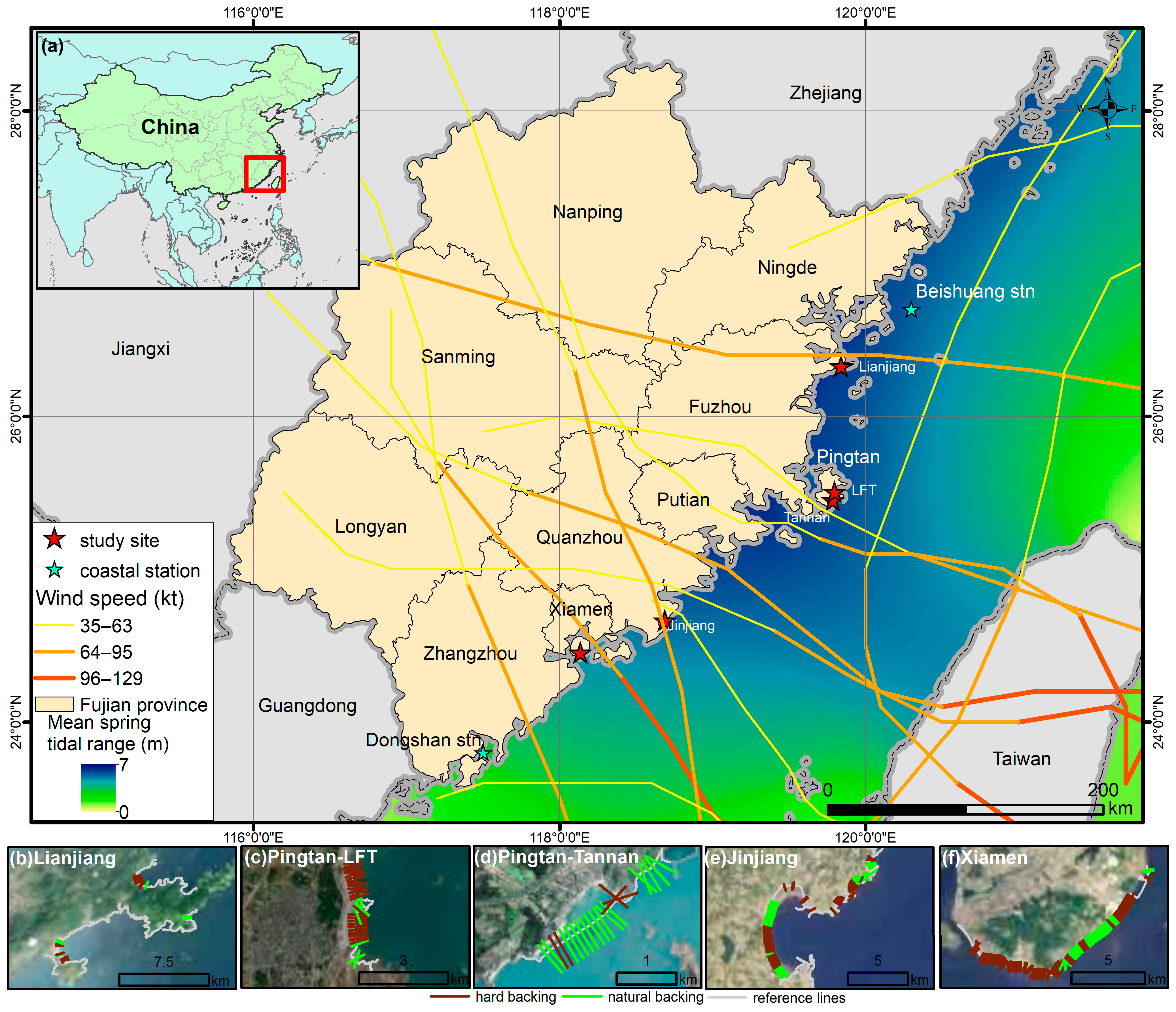
The Fujian coast faces the Taiwan Strait on the southeastern seaboard of China (Figure 1). Tides are semidiurnal and macrotidal. The EOT20 mean spring range, 2(M₂ + S₂), exceeds 4 m along the entire study coast. It peaks above 6 m in the funnel-shaped embayments between Lianjiang and Pingtan, where the predicted astronomical range reaches 7.4 m. Two wave climates alternate seasonally. From July to October the coast lies in one of the most typhoon-exposed sectors of the western North Pacific: nineteen typhoons passed within 250 km of the study sites during 2015–2026 alone, including the landfalls of Meranti (2016), Maria (2018) and Doksuri (2023). From roughly November to February, the northeast monsoon drives persistent moderate-to-high-wind seas along the Strait. Sandy beaches occupy pockets and embayed arcs between rocky headlands along an otherwise intensively developed coastline. Many are backed by seawalls, coastal roads, aquaculture-pond dikes or urban waterfronts.

Five beach sites in four coastal sectors were selected to span the regional gradients of exposure, orientation, backshore development and storm-track geometry (

Table 1. Characteristics of the five study sites, ordered from north to south.

Site	Facing	Character	Beach Transects (Natural/Hard) *	Scenes *	Median tanβ *	Site–Events (Resolvable/In Recovery)	Transects Per Event, Median (Range)	Validation Pairs	Key Storms
Lianjiang (Huangqi)	E	pocket beaches, aquaculture backdrop	22 (7/15)	344	0.10	4/4	22 (14–22)	0	Maria ‘18, Gaemi ‘24, Danas ‘25
Pingtan–Longfengtou (Pingtan-LFT)	NE–E	exposed urban tourist beach	31 (7/24)	270	0.11	4/0	3 (3–3)	5	Danas ‘25, Gaemi ‘24, Kong-Rey ‘24
Pingtan–Tannan	SE	sheltered embayed arc	22 (17/5)	184	0.09	6/3	8 (3–9)	6	Nepartak ‘16, Nesat ‘17
Jinjiang (Weitou Bay)	SE	mixed natural/armoured embayment	114 (48/66)	321	0.08	7/7	77 (22–103)	0	Doksuri ‘23 + 4 more
Xiamen	SE	nourished urban beaches	132 (39/93)	424	0.14	8/8	121 (52–127)	7	Meranti ‘16

* Beach transects are those retained in the final registry (Section 3.3), split by backshore class into natural and hard-backed. Scenes are usable shoreline detections of the strict extraction product. Median tanβ is the site median of the slope-confident transects. Resolvable site–events are those sampled by at least three registry transects in both event windows (Section 3.5); the recovery composite additionally requires eight (Section 3.6), which excludes Longfengtou. Validation pairs are the digitised reference waterlines that yield paired offsets (Section 3.4).

). From north to south, they are as follows. The east-facing pocket beaches on the southern shore of the Huangqi Peninsula in Lianjiang lie within 15 km of Maria’s landfall. Two contrasting beaches sample Pingtan Island: the east- to northeast-facing, exposed urban tourist beach at Longfengtou, and the sheltered, southeast-facing pocket-beach arc of Tannan Bay. These two are separated by only a few kilometres of headland and form a natural intra-island exposure contrast. The mixed natural–armoured beaches of the Weitou Bay embayment in Jinjiang (Quanzhou) are the closest site to Doksuri’s landfall. Southernmost, the urban beaches of southeastern Xiamen Island were struck directly by Meranti. Many of these beaches have been restored and artificially nourished since China’s first large-scale nourishment project at Guanyinshan in 2007 [30,31]. In situ observations are available from two stations of the Chinese marine observation network (https://mds.nmdis.org.cn), which report wind and pressure hourly and wave height every three hours. Beishuang, an offshore island station 70 km northeast of the Lianjiang site, recorded the landfall sea states of Maria; Dongshan lies in southern Fujian.

3. Data and Methods

The analysis proceeds in five stages. First, shorelines are extracted from the public Landsat and Sentinel-2 archive with the CoastSat toolkit (Section 3.1). Second, each shoreline is reduced to mean sea level using a global tide model and a beach-face slope inverted from the data itself (Section 3.2). Third, an expert-in-the-loop registry defines which transects sample a beach and classifies their backshore (Section 3.3). Fourth, the corrected series are validated against reference waterlines digitised from sub-metre imagery (Section 3.4). Finally, the validated series are analysed for the typhoon response, the post-storm recovery, and their environmental controls (Section 3.5, Section 3.6 and Section 3.7). Two recurring terms central to this study are defined as follows. First, the extraction workflow was executed under two quality-control configurations: a strict product, which underpins all time series, event-based statistics, and trends reported herein, and a relaxed product, utilised exclusively for validation pairing and mapping maximum SDS retrieval extent (Section 3.1). Second, tide gating refers to the exclusion of satellite observations acquired seaward of the slope break between the beach face and the low-tide flat, where a single-slope tidal correction becomes physically undefined. This slope break is empirically located in Section 4.1 and applied as detailed in Section 3.2. The complete analytical workflow is illustrated in Figure S1, and all associated parameter thresholds and processing windows are summarised in Table S1.

3.1. Satellite Imagery and Shoreline Extraction

Shorelines were extracted with the CoastSat toolkit, v3.3 [17]. CoastSat retrieves publicly available Landsat and Sentinel-2 scenes through the Google Earth Engine catalogue [32]. It maps the instantaneous sand–water interface at sub-pixel resolution, using a supervised image classification followed by MNDWI thresholding. We processed all available Tier-1 scenes from Sentinel-2 (10 m), Landsat 8, and Landsat 9—with Landsat multispectral bands pan-sharpened from 30 m to 15 m using the panchromatic band—acquired over the five study sites between January 2015 and June 2026 (Table 1). The two nominal spatial resolutions were deliberately not harmonised via resampling. Because CoastSat locates the waterline at sub-pixel resolution by thresholding a continuous index surface and interpolating contours between pixel centres, the detected shoreline position is not quantised to the pixel grid, and its accuracy is not dictated by pixel size alone. Downsampling Sentinel-2 to the 15 m Landsat grid would thus discard valuable spatial information without enhancing cross-sensor comparability. Instead, we treat cross-sensor consistency as a measurable variable and constrain it through two independent validation pathways: (1) sensor-by-sensor comparison against reference waterlines (Section 3.4), and (2) recomputation of the entire event matrix using Sentinel-2 imagery alone (Section 4.1). This period matches the high-frequency, multi-mission era required to resolve individual storm events. The pre-2015 archive was not used in the event analysis, because its effective revisit is insufficient for pre/post-typhoon pairing. Cloud masking followed the CoastSat defaults: a scene cloud-cover threshold of 0.15, an s2cloudless probability threshold of 40%, and a 300 m exclusion buffer around detected clouds. The standard September–October 2016 archive contained no usable scene of Xiamen around the landfall of Super Typhoon Meranti. We therefore additionally processed Landsat 7 ETM+ scenes for June 2016–January 2017. Despite the SLC-off stripe gaps, the between-stripe imagery yielded a usable post-Meranti, pre-Megi observation (21 September 2016) that would otherwise be missing. Stripe areas are simply masked as no-data by the toolkit.

Candidate shorelines were constrained by a reference shoreline built from the OpenStreetMap (OSM) coastline layer. This layer traces only the land–sea boundary. It therefore excludes the aquaculture ponds and other inland water bodies that are widespread behind the Fujian coast. Where a site’s coastline consists of several OSM segments, all segments intersecting the author-supplied beach polygons (Section 3.3) were retained. Cross-shore transects were then generated automatically every 100 m along the reference line. Each transect is oriented along the local shore normal, which is computed from the tangent of the reference line over a ±10 m window and directed landward-to-seaward. Each extends 200 m landward and 400 m seaward. The strongly asymmetric seaward reach is required because, at spring low tide, the waterline of these macrotidal beaches can lie more than 300 m seaward of the OSM line. Shorter, symmetric transects were found to truncate the low-tide portion of the signal. This procedure fixes the transect geometry from the reference line alone; the author’s manually digitised waterlines (Section 3.4) are used only to help decide which of these transects sample a sandy beach (Section 3.3), never to define the transect lines themselves.

Two extraction products were generated with different quality-control settings. Each is used only for the purpose it suits. The strict product (minimum mapped shoreline length 500 m; maximum distance from the reference shoreline 100 m) suppresses spurious detections. It is the basis of all shoreline time series, event statistics and trend estimates. The relaxed product (200 m and 250 m, respectively) recovers detections on short pocket beaches, which the 500 m length rule systematically removes. It also recovers waterlines far seaward of the reference line at low tide. It is noisier, and is therefore used only for validation pairing against reference waterlines (Section 3.4) and for mapping where SDS can and cannot be obtained on this coast. The two products were archived separately, so that every downstream result is traceable to one of them.

3.2. Tide Prediction, Beach-Face Slope, and Tidal Correction

The mean spring tidal range at the study sites reaches 5–7 m (Figure 1). The raw cross-shore position of the instantaneous waterline is therefore dominated by the tidal stage at acquisition time. Without correction, the tide alone displaces the waterline horizontally by several tens of metres. Tidal elevations at each acquisition epoch were predicted with the EOT20 global ocean tide model [33], evaluated at the closest wet grid cell to each site with the pyTMD software [34]. EOT20 is an independently published, peer-reviewed empirical tide model derived from multi-mission satellite altimetry, and is openly available. Two independent regional assessments support this choice for our setting. First, ref. [35] evaluated eight modern global tide models, including FES2014b and FES2022b, and one regional model against the tidal constants of 65 tide gauges in the eastern China marginal seas—the East China Sea, the Yellow Sea and the Bohai Sea, of which the East China Sea adjoins our sites to the north. They reported that EOT20 exhibited the highest accuracy, achieving the lowest root sum square (RSS) error of 11.1 cm and agreeing best with GPS-measured M₂ ocean tide loading displacements. Second, ref. [36] compared eight models against tide gauges in the same three seas and found the ranking to depend on setting: while NAO.99Jb excelled at eight offshore gauges, EOT20 proved superior at twenty-four island and coastal gauges—a domain closely mirroring our study sites—yielding the strongest M₂ agreement (13.03 cm root mean square) and the smallest root sum square (15.22 cm). The specific choice of tide model has limited leverage on our results, because the correction consumes only the predicted instantaneous elevations and the validation rests on same-day pairs whose offsets largely cancel any constant model bias. Predicted tides at the acquisition epochs of the 184–424 usable scenes per site span 73–76% of the full astronomical range. The sun-synchronous sampling of Landsat and Sentinel-2, accumulated over a decade, therefore captures most of the tidal excursion. The lowest spring-tide stages, below about −2.4 m relative to mean sea level, are however never observed at the ~10:30 local overpass time. This is a systematic blind spot of sun-synchronous SDS on this coast.

Shoreline positions were reduced to mean sea level (MSL) with the standard horizontal correction

Δx = z/tanβ

(1)

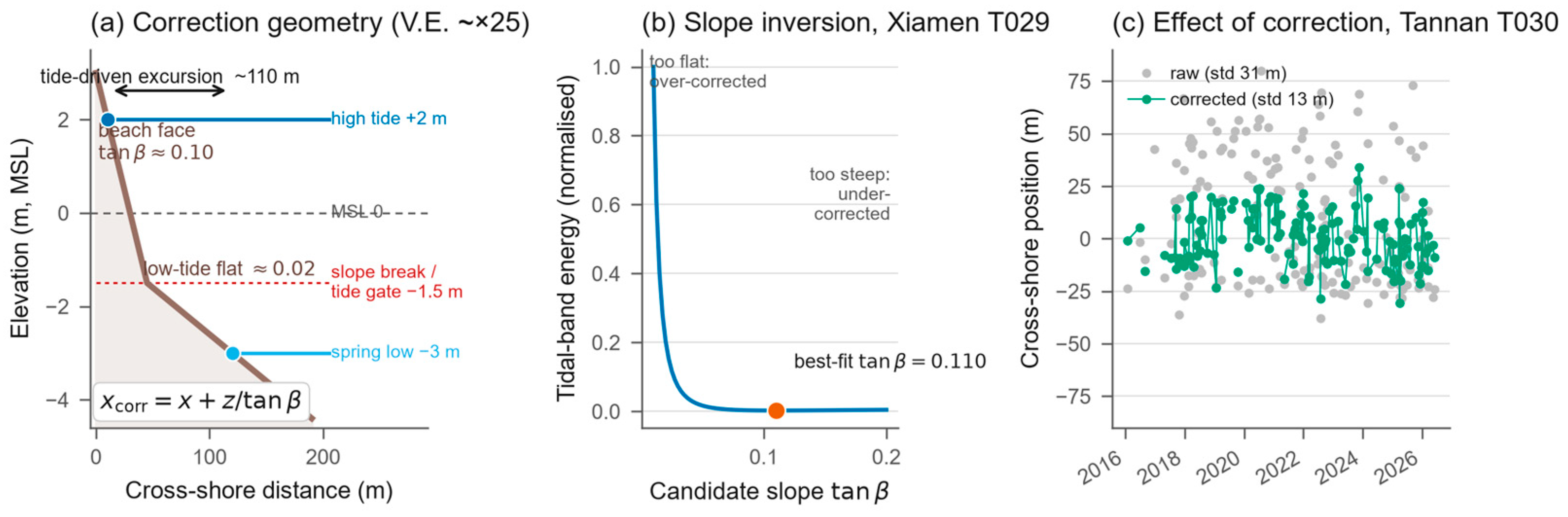
where z is the predicted tide and tanβ the beach-face slope (Figure 2a). Slopes were estimated per transect with the spectral method of [26]. The method selects the slope that minimises the energy of the corrected time series in the tidal alias frequency band. We searched slopes between 0.01 and 0.20 (step 0.0025), using the published Sentinel-2 settings. Slopes were inverted only on transects carrying at least 60 valid observations within the beach-face regime, following the removal of outliers exceeding three standard deviations from the transect median. An inversion estimate was considered converged if it fell at least two search steps within either parameter bound. Transects whose estimate converged inside the search interval (hereafter slope-confident) were corrected with their own slope. The estimates span 0.02–0.19, with site medians of 0.08–0.14. These values are consistent with surveyed slopes of comparable sandy beaches. Transects whose estimate saturated at a search boundary are those where the waterline is too tide-insensitive to resolve a slope, which occurs on rocky headlands and hard shorefronts but also on some steep beaches. Their own slope being unreliable, these transects were corrected with the site-median slope; whether such a transect samples a beach was decided by the registry (Section 3.3), not by this flag. At the Pingtan sites, observations acquired below a tidal stage of about −1.5 m were excluded from the corrected series (“tide gating”): below this stage the waterline crosses a slope break onto a low-tide flat far gentler than the beach face, so that a single beach-face slope no longer defines the correction (Section 4.1). Retaining these observations doubled the residual scatter.

3.3. Beach-Transect Registry and Backshore Classification

Analyses of beach behaviour require an explicit definition of which transects sample an actual sandy beach face. Each of the 100 m spaced transects defined in Section 3.1 was therefore classified as beach or non-beach; the classifier is the registry described below. The slope-confidence flag alone proved insufficient in both directions. Confident slopes occur on some non-beach shorefronts, such as aquaculture flats and harbour basins. Conversely, genuine pocket beaches fail the confidence test, because the strict product provides too few observations there. A transect registry was therefore assembled from four independent lines of evidence. First, all slope-confident transects were annotated one by one by the author, drawing on field familiarity with this coast; non-beach transects were explicitly rejected. Second, beach outline polygons digitised by the author for the Lianjiang and Jinjiang embayments were used as a mask. Third, any transect intersected by the author’s digitised waterlines from high-resolution imagery (Section 3.4) qualifies as beach. Fourth, single-transect gaps flanked by confirmed beach on both sides were interpolated. This yielded 362 candidate beach transects. Two further screens were then applied. Transects that a review against high-resolution imagery found not to be beach were removed (four transects). In addition, each transect was tested for geometric reliability: the angle between the transect and the local shoreline trend, taken through the origins of its neighbours, should be close to 90°. Transects deviating by more than 30°—a minority (37 transects) arising where the reference line is locally jagged—were excluded, because an oblique transect inflates the apparent cross-shore change by 1/cos of the deviation. The final analysed registry contains 321 beach transects. Excluding the oblique transects, or retaining them, changes the site-level event medians by at most about 1–3 m and alters none of the conclusions.

Each registry transect carries a backshore class, assigned from current high-resolution imagery and local knowledge. Natural denotes dune, vegetation or open ground behind the beach. Hard denotes a seawall, coastal road, promenade, buildings, concrete platforms, or aquaculture-pond dikes within ~50 m of the high-water line. The operational criterion is whether a hard structure prevents landward exchange. Reported nourishment history is recorded where known; in particular, the Xiamen Island beaches have been repeatedly restored and nourished since 2007 [30]. It is marked unknown elsewhere, since nourishment cannot be established from imagery alone.

3.4. Validation Against Reference Waterlines

SDS accuracy was assessed against waterlines digitised manually from sub-metre historical imagery in Google Earth Pro. From an inventory of all usable acquisitions over the Pingtan and Xiamen sites, 19 dates (2016–2024) were selected. Each digitised waterline was paired with a satellite acquisition as close as possible in time; the set includes seven same-day pairs and four pairs one day apart. The dates were also chosen to span low, mid and high tidal stages, so that the error could be resolved as a function of tide. The digitisation followed a fixed protocol. The operator traced the instantaneous water edge—the boundary between water, including swash and attached foam, and exposed sand. The high-water wet/dry mark was explicitly not traced. Rocky stretches and stream mouths were skipped. Each date includes two to three fixed control points on hard structures, used to quantify georeferencing offsets between image dates. For the satellite data, all imagery was projected to a common coordinate system (EPSG:32650), which also served as the spatial framework for the reference shoreline, transects, and digitised waterlines. Any scene with a reported georeferencing accuracy exceeding 10 m was discarded during extraction (Table S1). For the reference data, evaluated relative to their across-date centroids, the 56 control-point occurrences exhibit a median radial residual of 3.1 m and a root-mean-square residual of 5.0 m, with a maximum of 17.8 m (Table S2). Because this error metric inherently incorporates operator pointing precision—which cannot be isolated—it establishes an upper bound on the inter-date registration uncertainty of the reference imagery. This value remains an order of magnitude smaller than the low-tide offsets analysed in Section 4.1.

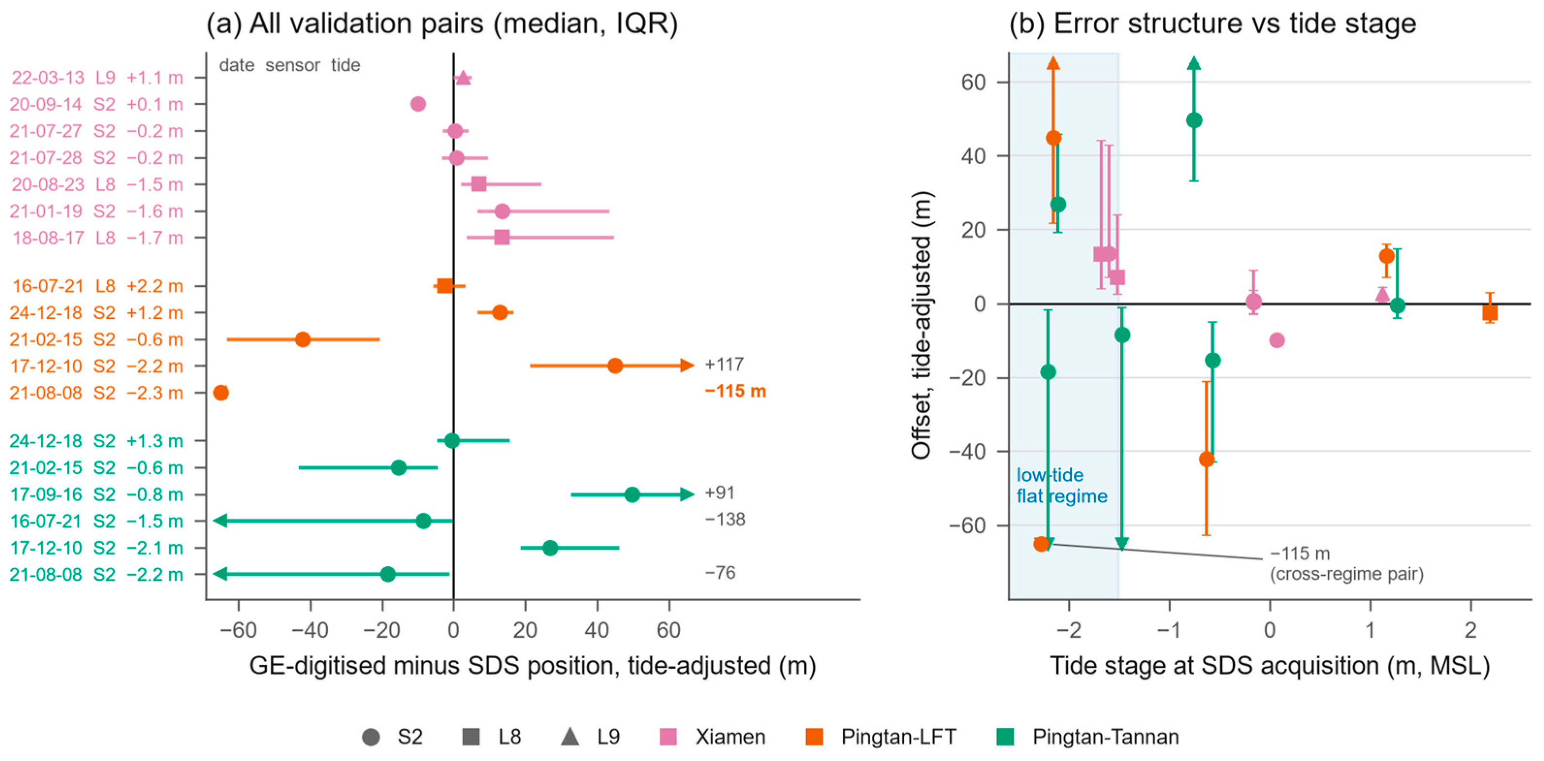
Among the 19 digitised waterlines, 18 produced valid paired offsets. Pairing required at least three transects intersected simultaneously by both the digitised waterline and the SDS shoreline. The Tannan waterline acquired on 24 March 2021, representing the shortest trace in the dataset, did not reach this threshold for any scene within the 20-day search window and is therefore omitted from Figure 3. Additionally, precise acquisition times for the commercial imagery were unavailable as they are not published within Google Earth. Tides for the digitised waterlines were therefore predicted for an assumed 10:30 local overpass. The residual time uncertainty was propagated as a horizontal envelope: the tide range over 09:30–11:30, divided by the local slope. Pairs whose envelope exceeds 15 m are flagged and interpreted separately.

Offsets were computed along the registry transects as the difference between the digitised waterline and the SDS waterline of the paired scene. The digitised position was first adjusted to the tidal stage of the satellite acquisition, using the transect slope. At low tide, a single scene’s water–land contour often meets one transect at several points. The wide exposed flat is dissected, with emergent sand ridges alternating with water in runnels and pools, and wet backshore patches or swash foam can also register as water. For each transect we compared the crossing nearest the digitised waterline, and recorded the number of crossings as a quality flag. The relaxed extraction product was used for this pairing (Section 3.1). Positive offsets denote an SDS shoreline position landward of the reference waterline, which is opposite to the seaward-positive convention adopted for the event responses in Section 3.5. Furthermore, the evaluation dates were selected to encompass low, mid, and high tidal stages—defined here as low (below −1 m), mid (−1 to +1 m) and high (above +1 m) relative to mean sea level—so that the error could be resolved as a function of tide.

3.5. Typhoon Catalogue and Event-Response Analysis

Storm events were taken from IBTrACS v04r01 [37]. We selected all systems of 2015–2026 that passed within 250 km of any site with a peak intensity of at least 64 kt. This yields 19 typhoons and, per site, 5–12 candidate events within 150 km. For every site–event pair, the beach state before and after the storm was estimated on each registry transect. The pre-event state is the median corrected position within −45 to −2 days; the post-event state is the median within +2 to +30 days. The event response Δx is the post-event position minus the pre-event position, measured along the transect with the seaward direction positive; a landward, erosional shift is therefore negative. The site-level response is the median of Δx across transects with at least one observation in each window. Events whose pre-event window contains another catalogued typhoon are flagged as compound and interpreted accordingly. The window lengths trade the sparse revisit—about 1–3 usable observations per month per transect—against contamination by unrelated variability. The +30-day post window measures the persistent event signal, rather than the instantaneous post-storm scarp, which the revisit cannot guarantee to sample. Because the windows pool scenes from different sensors, whose relative biases were quantified in the validation, we verified the event matrix against sensor mixing; the result is reported in Section 4.1.

3.6. Recovery Analysis

Post-typhoon recovery was analysed with superposed-epoch analysis [38], a standard compositing technique that aligns many events on a common reference time and extracts their shared signal. It is robust to the low signal-to-noise ratio of individual transects. We analysed every site–event resolved by at least eight registry transects, retaining only those transects that exhibited erosion of at least 5 m within the event window (Δx₀ ≤ −5 m, measured over +2 to +30 days as in Section 3.5). The pre-event baseline was defined as the median position over the 60 days prior to the storm. This baseline window is longer than the 45-day window used for event response assessment in Section 3.5; because recovery trajectories extend up to 240 days, a longer baseline minimises the influence of individual pre-event scenes on the overall normalised trajectory. The eight-transect threshold ensures that the composite response is derived from a representative transect population. This criterion filters the 29 resolvable site–events from Section 3.5 down to 22, excluding Longfengtou Beach entirely, where sparse strict-product coverage restricts all events to a maximum of three transects (Section 5.4). Consequently, the composite profile represents four of the five study sites. All parameter values are detailed in Table S1. All subsequent corrected positions were expressed as a fraction of the local event displacement (r):

r = (x(t) − x_pre)/|Δx|

(2)

In this normalisation, −1 corresponds to the post-storm state and 0 to full recovery. Trajectories were truncated at the next catalogued event (minus two days) or at 240 days, whichever came first. The 5638 normalised observations from 22 site–events were binned by time since the event. Time-bin boundaries (2, 20, 40, 60, 90, 120, 160, 200, and 240 days; Table S1) were configured with higher temporal resolution during the early post-storm phase—where recovery dynamics are most rapid—and progressively wider intervals thereafter to maintain comparable sample counts per bin. Normalised displacements exceeding ±6 were discarded as gross outliers, and bins holding fewer than ten observations are not reported. Composite values reported herein reflect the binned data as plotted; Table S3 reproduces the composite profile using an alternative binning scheme, confirming that the overall curve shape, trough position, and endpoint are unchanged. Finally, to isolate the seasonal control suggested by the raw composite, the stack was split by event month (July–August versus September–November typhoons). It was additionally projected onto calendar month. An exponential recovery model, the standard description for wave-dominated coasts [8], was fitted to the composites for comparison with published recovery timescales.

3.7. Wave Forcing and Group Contrasts

Event wave forcing was characterised from two sources. ERA5 hourly fields of significant wave height, mean wave direction and peak period (2015–2026) [39] were extracted at the nearest wet 0.5° grid cell to each site. Coastal-station observations at Beishuang and Dongshan, giving hourly wind and pressure and three-hourly wave height, serve as an in situ check on ERA5 and document the landfall sea states. Both stations provide continuous monthly records from 2010 to 2025, spanning every analysed event. At the peak of Typhoon Maria (11 July 2018, 06:00 local), Beishuang recorded a significant wave height of 9.1 m at a 15 s period, as station pressure fell to 963 hPa. Three forcing metrics were tested against the site–event responses: the peak significant wave height in a ±2-day window; its onshore component relative to the mean shore normal of the site’s registry transects; and an event-integrated onshore wave-energy proxy (E):

E = Σ H_s² T_p cos(θ)

(3)

where H_s is the significant wave height, T_p the peak period, and θ the angle between the mean wave direction and the shore normal, with offshore-directed hours (cos θ < 0) set to zero. The product H_s² T_p is proportional to the deep-water wave energy flux. The natural- versus hard-backed contrast was evaluated within events. For each site–event with at least three transects in each class, the paired difference of class medians was tested with the Wilcoxon signed-rank test. This pairing controls for the shared forcing of the two classes in the same event. All processing used Python (CoastSat v3.3, pyTMD, xarray, GeoPandas).

4. Results

4.1. SDS Accuracy and Applicability on a Macrotidal Coast

Predicted tides at the 184–424 usable acquisition epochs per site span 73–76% of the full astronomical range. The decade-long, sun-synchronous archive therefore samples most of the tidal excursion. The exception is systematic rather than random. Stages below about −2.4 m (relative to mean sea level) never coincide with the ~10:30 local overpass. The lowest spring-tide foreshore is therefore invisible to Landsat and Sentinel-2 on this coast. Beach-face slopes inverted from the tidal-band minimisation (Figure 2b) converge on the 321 registry transects that sample beaches. The values span 0.02–0.19, with site medians between 0.08 (Jinjiang) and 0.14 (Xiamen). Applying the per-transect corrections reduces the median scatter of the beach time series by 36–49% at four of the five sites, from 11–25 m to 7–16 m (compared on the same observations). At the exposed Longfengtou Beach, where slope-confident transects are scarce and the applied slope is therefore poorly constrained, the correction is largely ineffective (19.7 to 19.3 m). The residuals at the other four sites are comparable to, or smaller than, the 10–30 m displacements produced by the strongest typhoons (Figure 2c).

The comparison against the 18 digitised reference waterlines that yield paired offsets resolves how the remaining error is structured (Figure 3). At mid-to-high tidal stages the SDS is essentially unbiased at all validated sites. At Xiamen, two reference waterlines digitised on consecutive days are both compared with the same Sentinel-2 scene, and agree with it to +0.3 m and +0.7 m (n = 56 transects each). The Landsat-9 next-day pair agrees to +2.7 m. The high-tide Landsat-8 pair at Longfengtou (tide +2.2 m) agrees to −2.5 m, and the same-day Tannan pair at +1.3 m tide to −0.5 m. The consecutive-day pair at Xiamen provides an independent check of the slope used in the tidal adjustment. The two reference waterlines were digitised one day apart, across a 0.6 m tide step, with negligible morphological change. Measured against the same Sentinel-2 scene they lie 4.8 m apart, which implies a beach-face slope of 0.13—within about 7% of the slope obtained by inversion.

Toward low tide, the error grows into a systematic landward bias of the SDS. At Xiamen (median slope 0.14), the low-tide pairs give +7.0 m (Landsat-8, same day), +13.5 m (Sentinel-2) and +13.4 m (Landsat-8, 17-day separation). On the flatter Pingtan beaches the low-tide bias is larger: +26.9 m at Tannan (slope ≈ 0.09) and +45.0 m at Longfengtou. The Longfengtou pair has a wide interquartile range 22–117 m, with multiple SDS crossings on six transects. This reflects the coexistence of beach-face and flat-edge detections in a single scene. Mid-tide pairs at the Pingtan sites scatter between −42 m and +50 m. These pairs are the most sensitive to the unknown commercial-imagery acquisition time: on slopes of 0.05–0.10, a ±1 h timing uncertainty alone maps to a ~11–15 m horizontal envelope. They are therefore treated as bounding cases rather than bias estimates. The overall bias structure is consistent with the known landward migration of index-based waterlines over wet, low-tide foreshores, scaled by the inverse of the local slope.

Below the slope break, the tidal correction is no longer valid, and the residual it leaves constrains the geometry of the lower profile. The cross-regime pair at Longfengtou compares a high-tide reference waterline (+2.1 m) with a spring-low SDS acquisition (−2.3 m). It leaves a residual of −115 m after adjustment with the beach-face slope. This back-solves to an effective slope of ≈0.02 for the lower profile: the waterline has migrated onto a low-tide flat an order of magnitude flatter than the beach face (Figure 2a). This motivates the −1.5 m tide gate applied in Section 3.2. Gated observations amount to 8–13% of the archive at the Pingtan sites.

Taken together, across the two sites with digitised reference waterlines, the applicability envelope of tidally corrected satellite-derived shorelines (SDS) is bounded in three main respects. Vertically, the method is unbiased above roughly mean sea level. It degrades to a slope-dependent landward bias of ~7–45 m in the lower intertidal. It fails below the beach-face/flat transition, which the sun-synchronous sampling largely avoids in any case. Horizontally, the standard quality controls suppress genuine detections on pocket beaches shorter than the 500 m minimum shoreline length. Mid- and high-tide detections are also sparse on the urban Longfengtou Beach. Both losses are recoverable with relaxed controls, at the cost of noise. This is why the relaxed product is reserved for validation pairing and coverage assessment, rather than time-series analysis. Within this envelope, the corrected series resolve event-scale beach change of order 10 m and above when aggregated as multi-transect medians. That capability is the basis of the analyses that follow.

Sensor differences are not detectable above the tide-driven structure. At mid-to-high tidal stages, where the slope-driven low-tide bias is absent, the nine Sentinel-2 pairs give a median offset of −0.1 m, while the single Landsat-8 and Landsat-9 pairs within that tidal band exhibit offsets of −2.5 m and +2.7 m. Although the validation dataset is too unevenly distributed across sensors (fifteen Sentinel-2, three Landsat-8, and one Landsat-9 pair) to justify a formal sensor-by-sensor performance comparison, the observational error is predominantly governed by tide stage rather than sensor type. Consequently, the Sentinel-2-only recomputation presented below serves as a more rigorous test of the validity of cross-sensor mixing. The event analysis pools scenes from different sensors, so we verified that the sensor biases quantified above do not contaminate it. Recomputing all resolvable site–event responses from Sentinel-2 scenes alone reproduces the all-sensor values with a median absolute difference of 0.8 m (90th percentile 3.6 m, n = 17 site–events). The single larger departure—Maria at Lianjiang, 10 m—occurs at the smallest site–event (15 transects, 1–3 scenes per window) and lies within that event’s interquartile range, reflecting scene-sampling variance rather than a sensor artefact.

4.2. Typhoon Response and Its Geometric Organisation

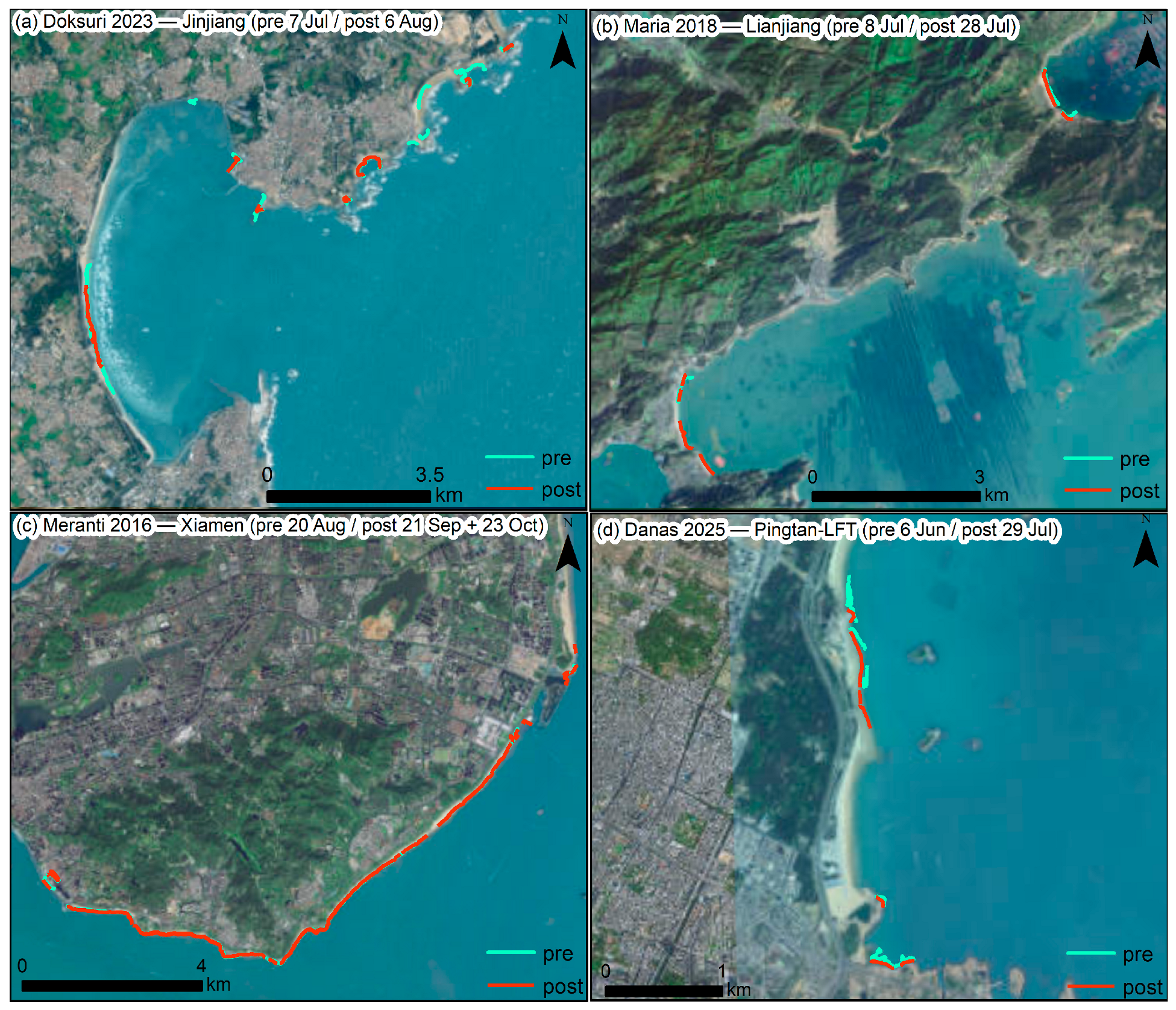
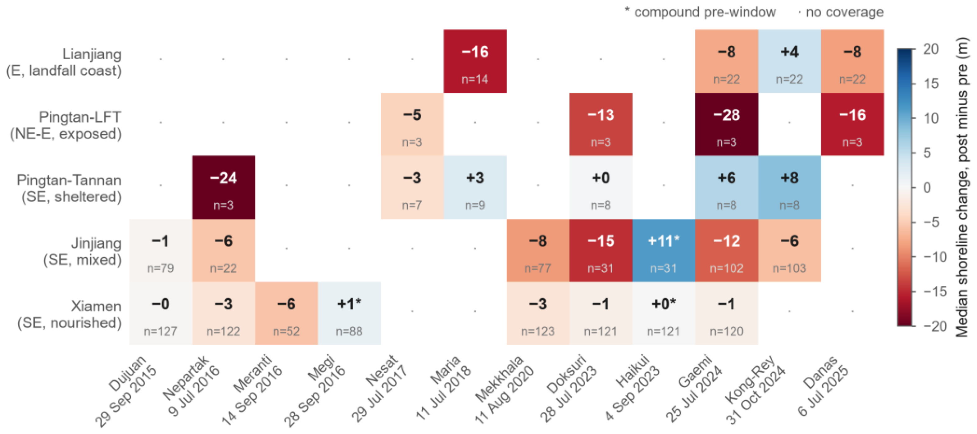
Sampling is strongly uneven between sites (Table 1). The two largest sites carry 77 and 121 transects per event, whereas Longfengtou reaches only three in each of its four resolvable events and contributes nothing to the recovery composite. Across the 19 catalogued typhoons and five sites, 29 site–event responses could be quantified. The strongest signals are unambiguous erosion. The four flagship landfalls are mapped as pre- and post-event shorelines in Figure 4, and the complete set of responses is summarised in Figure 5. Doksuri (2023) made landfall 33 km from Jinjiang as the strongest storm to strike Fujian since 2016. It displaced the Jinjiang beach waterlines landward by a median of 15 m (interquartile range 8–20 m, n = 31 transects). Maria (2018) produced a median 16 m retreat on the east-facing beaches of the Huangqi Peninsula, within 15 km of its landfall (interquartile range 0–20 m; n = 14 transects sampled by 1–3 scenes per window). The exposed Longfengtou Beach on Pingtan Island eroded in every resolved storm, by 14 m during Doksuri (2023), 28 m during Gaemi (2024) and 16 m during Danas (2025). Its sparse strict-product coverage there limits each estimate to three transects. Super Typhoon Meranti (2016), the most intense storm in the catalogue (local intensity ~110 kt), left a comparatively modest but robust 6 m median retreat across 52 Xiamen transects. This damped response is consistent with the restored and nourished, steep urban beaches of Xiamen Island, whose median event responses never exceed 6 m in any of the eight storms sampled there.

The size of each response, however, is not set by the storm’s intensity, and only weakly by its distance. It depends mainly on geometry: the direction from which the storm strikes, and the orientation and exposure of each beach. The clearest demonstration is the single-storm, cross-site gradient of Gaemi (2024), which passed within 30–140 km of all five sites. Its response ranges from −28 m at the northeast-facing, exposed Longfengtou, through −12 m and −8 m at Jinjiang and Lianjiang, to −1 m at nourished Xiamen—and to +6 m (accretion) at the sheltered, southeast-facing Tannan embayment. The same pattern appears within a single island. Longfengtou and Tannan are separated by only a few kilometres of headland. Yet across the shared event set, Longfengtou eroded in every resolved storm (−5 to −28 m), while Tannan showed null-to-positive responses (0 to +8 m) in all but two storms—Nepartak (2016) and Nesat (2017), whose tracks placed Tannan on the onshore-wind side. During Gaemi the contrast was extreme: 28 m of erosion at Longfengtou against 6 m of accretion at Tannan, a few kilometres away. This indicates intra-island sediment redistribution, with storm waves refracting into the sheltered embayment, rather than a simple presence or absence of impact.

The site-level responses demonstrate strong robustness to the selection of event windows. Re-evaluating the computations across alternative pre-event windows (30 and 60 days) and post-event windows (21 and 45 days) preserves the sign of all response magnitudes ≥ 12 m, with a minimal median shift of only 2.0 m (Table S4). All sign reversals are confined to responses below 12 m—a threshold at or within the baseline series scatter reported in Section 4.1. The cross-site gradient observed during Typhoon Gaemi, including the sign reversal between Longfengtou and Tannan, is consistently reproduced under every parameter configuration. Consequently, we treat responses of approximately 12 m or greater as fully resolved, while regarding near-null responses as individually uninformative.

Two factors that might be expected to control the responses do not do so consistently. The first is offshore wave forcing. The ERA5 peak significant wave height in a ±2-day event window does not correlate with the observed displacements (Spearman ρ = +0.10, p = 0.60, n = 29 site–events), and neither does the event-integrated onshore wave-energy proxy (ρ = +0.13, p = 0.51). The onshore component of the peak wave height does show a weak positive correlation (ρ = +0.37, p = 0.049). 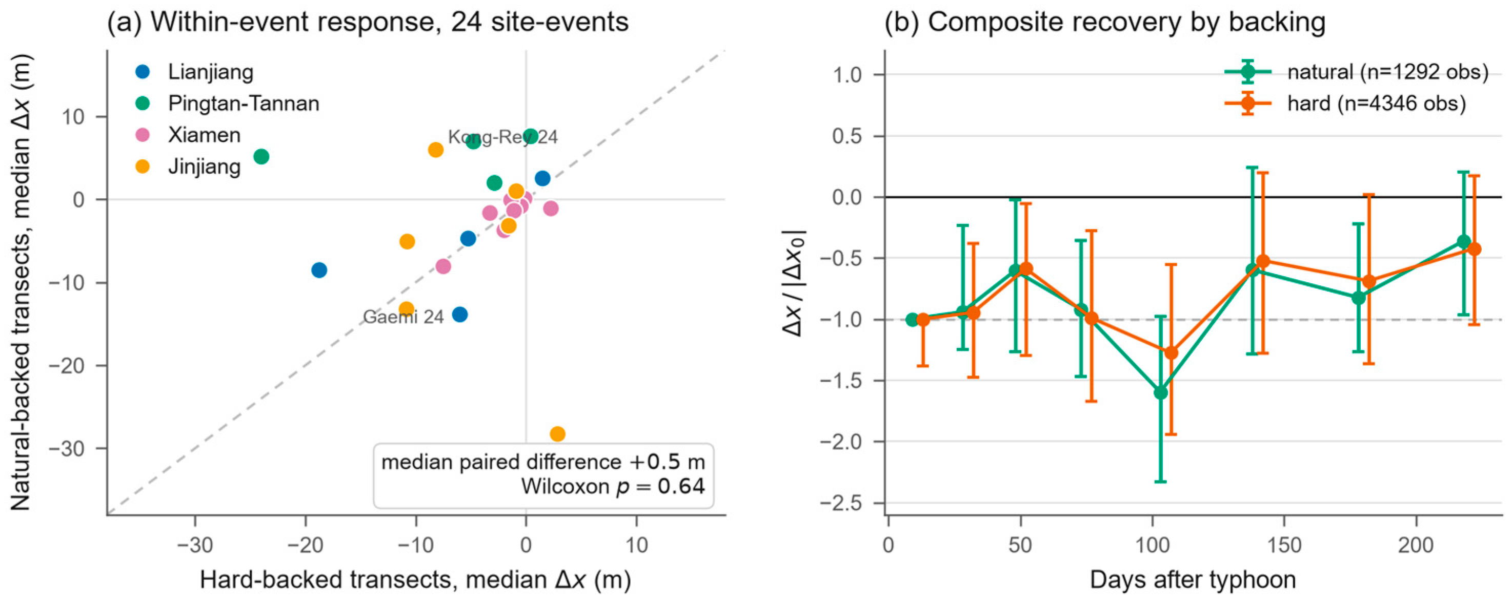That association is, however, the opposite sign to a wave-erosion forcing relationship—larger onshore waves would drive more, not less, erosion—and it does not survive the removal of compound events (p = 0.066). We therefore find no consistent offshore wave-forcing control of the response. The positive sign is instead consistent with a geometric confound, in which sheltered embayments accrete under the same onshore-directed waves that erode the exposed beaches. The in situ record confirms the forcing itself was substantial: Beishuang station measured a 9.1 m significant wave height at Maria’s closest approach. The absence of a predictive relationship thus reflects the failure of “offshore, untransformed” wave metrics on a strait-sheltered, crenulated coast, not the absence of wave forcing. The second factor is the backshore class, which does not change the immediate response. Across 24 site–events with at least three transects in both classes, the median paired difference between natural- and hard-backed segments is +0.5 m (Wilcoxon p = 0.64; Figure 6a). Individual events scatter in both directions. At the event scale on this coast, where a beach lies—its exposure, orientation, and position relative to the storm track—matters far more than what stands behind it, or how large the offshore sea state was.

4.3. Post-Typhoon Recovery and Its Monsoon Gating

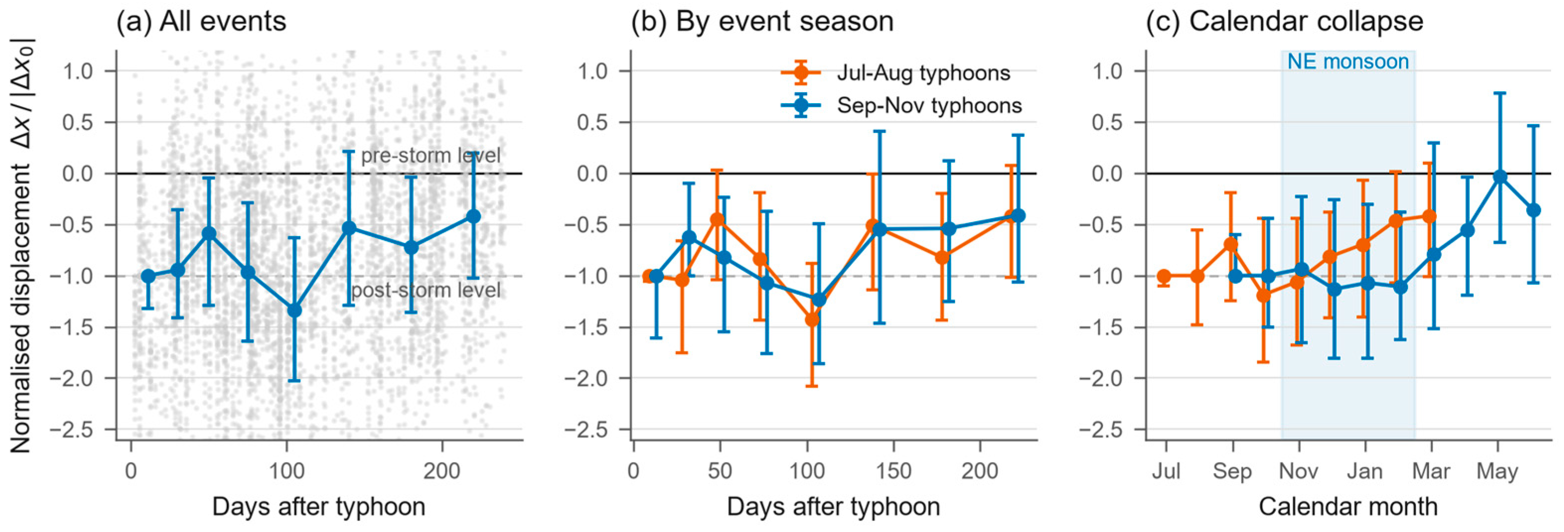
The superposed-epoch composite of all eroded beach transects departs strongly from exponential relaxation (Figure 7a). The normalised displacement recovers only partially during the initial calm window—reaching a median of −0.59 in the 40–60 day bin—before re-intensifying to its most eroded composite state (median of −1.33 in the 90–120 day bin), which is more eroded than the immediate post-storm position approximately three months following the events. Recovery resumes only thereafter, reaching −0.4 (about 60% of the loss) by the 240-day truncation limit. Consequently, an exponential model fit to this trajectory is rejected: the fitted timescale saturates at the imposed 400-day upper bound with negligible explanatory power (r² = 0.24), primarily because the trajectory is intrinsically non-monotonic.

Splitting the composite by event season shows that the non-monotonic shape is a calendar effect (Figure 7b,c). Beaches struck by July–August typhoons recover only partially during the calm early autumn (to −0.69 in September). They are then held or re-eroded through the winter (−0.82 in December), and have recovered to about −0.4—roughly 60% of the loss—by the end of their 240-day windows in March. Beaches struck by September–November typhoons behave differently. The shoreline positions remain suppressed near the immediate post-storm level throughout the northeast monsoon (median of −0.94 in November). Recovery is initiated only with the onset of the calm season, approaching near-complete recovery by late spring (−0.03 in May), despite some month-to-month variability in the composite. Projected onto calendar month rather than days-since-event, the two groups follow the same seasonal timing: shoreline positions are sustained at or below post-storm levels from October through February and recover exclusively during the subsequent calm season. The primary distinction between the two groups lies in magnitude rather than phase: the July–August group maintains a normalised position approximately 0.3 higher across the shared months, consistent with partial recovery achieved during the calm window preceding the monsoon. Displacement is held at or below the post-storm level from October through February, the months of the northeast monsoon in the Taiwan Strait. Recovery advances only during the calm seasons that flank the monsoon—the summer inter-typhoon windows and the following March–June spring. Shoreline recovery along this coast is thus gated by the seasonal monsoon calendar, rather than governed by the time elapsed since a storm. This gating is not produced by the compound events in the catalogue. Excluding the three site–events whose pre-event window contains an earlier catalogued typhoon leaves 4344 of the 5638 normalised observations, from 19 of the 22 site–events. Because all three excluded events belong to the September–November group, the July–August composite remains completely unchanged. Within the September–November group, suppressing these prior events actually intensifies the northeast-monsoon pinning rather than weakening it, while both the composite trough position and the 240-day endpoint remain invariant (Table S5). Contamination by subsequent typhoons is excluded by construction, since every trajectory is truncated at the next catalogued event.

The event catalogue provides one direct, within-season confirmation of the fast branch of this cycle. At Jinjiang, the event window of Haikui (September 2023) opens five weeks after Doksuri’s 15 m erosion and is flagged as compound. It registers a median rebound of +11 m (n = 31 transects). Because the two successive storms occurred only 38 days apart, this estimate is sensitive to the pre-event window selection: the standard 45-day baseline window overlaps the landfall of Typhoon Doksuri by seven days, thereby blending pre- and post-Doksuri shoreline states and rendering the +11 m value a conservative estimate. A 30-day pre-event window confined entirely within the inter-event interval yields a higher rebound of +16 m (Table S4). Most of the Doksuri loss was therefore restored within the summer calm window that followed. The recovery was rapid because Doksuri struck early in the season, ahead of a calm window; the same erosion occurring later in the year would instead have been carried across the monsoon into the following spring. It is this dependence on calendar position, not on elapsed time, that the gating describes. Finally, the backshore class does not detectably alter the recovery trajectory. The natural- and hard-backed composites track each other through the monsoon minimum and the spring recovery, within their interquartile ranges (Figure 6b). At most, the natural-backed segments show a suggestion of a deeper monsoon excursion. Both the storm response (Section 4.2) and the recovery are therefore organised by where a beach sits—in the coastal geometry and in the seasonal wave calendar—not by the presence of backshore structures.

5. Discussion

5.1. SDS on Macrotidal Coasts: An Error Structure, Not an Error Bar

The validation resolves the macrotidal accuracy problem identified by the benchmarking literature [21] into a structure with three distinct zones. Above roughly mean sea level, the tidally corrected SDS is unbiased at the few-metre level. This matches published microtidal performance [17,21], even on beaches fronting a 7 m spring range. In the lower intertidal, a landward bias emerges and grows toward low tide. It reaches ~7–14 m on a steep urban beach and 27–45 m on flat natural beaches. This is consistent with the wet-sand migration of index-based waterlines reported on other macrotidal and high-energy coasts [28,29]. Below the beach-face/low-tide-flat transition, the single-slope correction fails structurally: the waterline leaves the surface whose slope the correction assumes. On tide-modified profiles this failure is a property of the morphology [10], not of any particular detection algorithm. We therefore suggest that SDS accuracy statements on macrotidal coasts should be conditioned on tide stage, rather than quoted as a single RMSE. The three-zone envelope—unbiased, slope-scaled bias, regime failure—is established here at two sites only. Whether it transfers to other tide-modified coasts, or indeed to our own two unvalidated sites, is a hypothesis that site-specific validation would have to test. Our reliance on mean sea level as the reference datum is further supported by independent evidence that MSL is the optimal proxy shoreline for large-scale SDS applications across beach types [29].

The processing consequences are captured in four adaptations, which together form a practical protocol. First, per-transect slope inversion [26], with the boundary-saturation behaviour used as an automatic non-beach screen. Second, a tide gate excluding observations below the slope break. Third, dual strict/relaxed extraction products, separating time-series quality from coverage assessment. Fourth, an expert-in-the-loop transect registry that combines the slope screen with local geomorphological knowledge. In our case the registry corrected both false positives (tide-responsive aquaculture flats) and false negatives (pocket beaches suppressed by shoreline-length thresholds). None of these steps requires in situ data, which is what makes them inexpensive to attempt on the many macrotidal coasts where SDS is currently applied unvalidated [22,23]. We stress that this lowers the cost of validation rather than removing the need for it: the error magnitudes we report are specific to these beaches and their slopes. Two further caveats are specific to the observation system. Sun-synchronous acquisition never samples the lowest spring-tide stages (here, below −2.4 m), so the low-tide terrace is systematically invisible. And commercial-imagery acquisition times, needed for tidal adjustment of validation data, are not distributed with consumer platforms; this contributes a slope-dependent uncertainty that we bounded explicitly (±12–17 m on flat beaches).

5.2. Geometric Organisation and the Limits of Offshore Wave Metrics

Offshore wave forcing shows no consistent relationship with the response. Peak wave height and integrated wave energy are uncorrelated with it, and the onshore component correlates only marginally—and in the wrong direction, larger onshore waves accompanying less erosion rather than more (Section 4.2). This contrasts with the wave-energy scalings that perform well on open, swell-exposed coasts [3,6], and we interpret it as a property of the setting rather than of the data. Between the offshore ERA5 cell and any particular beach lie the sheltering of the Taiwan Strait, headland-and-embayment topography with strong refraction and diffraction, and a macrotidal water-level modulation that determines which part of the profile the waves attack. The same offshore sea state can therefore deliver onshore wave energy differing by an order of magnitude between neighbouring beaches. The five sites are not replicates of one coastal type, and the contrast between them is what makes the gradient legible. Lianjiang occupies the east-facing, exposed southern shore of the Huangqi Peninsula, a few kilometres from Maria’s landfall. Longfengtou is an open, east- to northeast-facing urban beach on the exposed coast of Pingtan Island, while Tannan, a few kilometres to the south, is a curved, southeast-facing embayment sheltered by a prominent headland and retains a semi-natural backshore. Jinjiang is a mixed natural and armoured embayment facing southeast across Weitou Bay. Xiamen’s beaches are pocket and urban beaches on a partly sheltered island, repeatedly nourished since 2007 [30]. Median beach-face slopes follow this ordering, from 0.08 on the open Jinjiang bay to 0.14 on the steep, nourished Xiamen beaches. Storm response tracks shoreline aspect and shelter rather than site size or transect count: the two Pingtan beaches, sharing a tidal regime and a wave climate, respond with opposite sign to the same storm.

The single-storm gradients demonstrate this directly. Gaemi (2024) produced responses from −28 m to +6 m across five sites, including opposite-signed responses on two beaches of the same island a few kilometres apart. Exposure and orientation relative to the storm track appear to organise the response more strongly than wave magnitude does. This is consistent with embayed-beach behaviour documented on storm-dominated coasts, where planform position and rotation dominate over bulk forcing [40], but here it operates at the scale of an entire multi-site coastline. A practical implication for regional management follows. On crenulated macrotidal coasts, a first-order screen for typhoon vulnerability should map which beaches face which track corridors, rather than apply offshore wave thresholds. Resolving the residual forcing dependence would require nearshore wave transformation modelling, which we identify as the natural next step.

The absence of a backshore effect on the immediate response (paired difference +0.5 m, p = 0.64) adds an event-scale data point to the coastal-squeeze debate [41,42]. Passive erosion in front of hard structures is a chronic mechanism; active scour amplification is an event-scale one. Our result indicates that on these beaches the event-scale amplification, if present, is smaller than the ~5 m resolution of the paired test. It does not address the chronic dimension. Whether hard-backed segments lose width over decades cannot be answered by a ten-year event analysis, and remains open for this coast. The restored and nourished Xiamen beaches [30] never eroded by more than 6 m in eight storms, including a direct landfall of the most intense storm in the catalogue. Their damped response suggests, conversely, that maintained sediment volume is an effective event-scale buffer. This observation is consistent with nourishment experience elsewhere [43]. With the present data, however, we cannot separate the contributions of nourishment, beach steepness and the island’s partial sheltering.

5.3. Monsoon-Gated Recovery

The recovery composite is, to our knowledge, among the first event-population descriptions of post-typhoon beach recovery on a monsoon-modulated macrotidal coast. It does not resemble the exponential relaxation established on mid-latitude swell coasts [5,8,9]. Recovery here is gated by the wave calendar. A fast branch operates in the calm summer and early-autumn windows; it restored most of a 15 m storm loss within about five weeks in the one directly observed case. The northeast monsoon (roughly November–February) holds or deepens the post-storm state, regardless of when the storm occurred. Completion is deferred to the March–June calm season. That both event groups reach this inflection at the same point in the calendar, despite storm timing separated by two to four months, is the clearest evidence for seasonal gating. They differ in level rather than in phase—the July–August group sits about 0.3 higher through the shared months, consistent with its having used a calm window before the monsoon arrived. It implies that “recovery time” is not a beach property on this coast: the same beach recovers in weeks or in eight months, depending on where in the calendar the storm lands. Seasonal shoreline cycles of comparable amplitude are well documented, including from satellite observations [18,26]. Their role as the rate-limiting gate for storm recovery, however, is a regime feature of typhoon–monsoon coasts that deserves testing elsewhere in East and Southeast Asia.

Independent observations elsewhere on the Chinese coast are consistent with a calendar control. At a headland–bay beach in Zhejiang, two typhoons in September 2022 were followed by a recovery that restored the volume lost to the second storm but left the beach short of its pre-first-storm state [12]: a late-season sequence that ended the year in deficit, as gating by the wave calendar implies it should. We frame this finding as observational consistency rather than definitive confirmation, as that study evaluated volumetric budget changes at a single embayment rather than tracking shoreline position across a broad event population.

Two management corollaries follow directly. First, beaches struck by late-season typhoons carry their deficit through the entire monsoon. Compound trajectories—a late typhoon followed by monsoon erosion—therefore produce the deepest and longest-lived beach loss. Early-warning and post-storm assessment should treat storm timing, not only storm magnitude, as a risk factor. Second, the March–June window is the natural season for nourishment and dune works, when natural recovery assists rather than fights intervention. Under a warming climate, projected shifts in the seasonal timing of typhoons [11] would change how many storms strike early enough to use the summer calm window before the monsoon. Storms that miss that window carry their deficit through the entire monsoon, as the September–November group does here, so the beach spends far more of the year in an eroded state. The seasonal composites presented here (Figure 7b,c) provide the baseline against which such a shift could be measured.

5.4. Limitations and Outlook

The primary limitation of this analysis rests on the spatial extent of the empirical validation. Reference waterlines were digitised at Pingtan and Xiamen, where the sub-metre historical archive is densest; Lianjiang and Jinjiang carry no independent validation, and every quantitative accuracy statement in this paper should be read as applying to the two validated sites. The beach-face slopes of the two unvalidated sites bracket the validated range differently. Lianjiang, at a site-median slope of 0.10, lies within the 0.09–0.14 spanned by the validated sites, so applying the error structure of Section 4.1 there is an interpolation. Jinjiang, at 0.08, is marginally flatter than any validated site; because the low-tide bias scales as the inverse of the slope, the bias there would be expected to be about a tenth larger than the flattest value we measured, so our reported envelope is, if anything, slightly optimistic for that site. We emphasise that both deductions rely on similarity arguments rather than direct measurement, and thus cannot substitute for site-specific empirical validation.

Four further limitations bound the present analysis. First, tidal predictions rely on a global model (EOT20), validated regionally against altimetry but not against mainland Fujian tide gauges, whose records were not accessible to this study. The validation design—same-day pairs and tide-adjusted offsets—limits the leverage of any model bias, but a gauge-based check would strengthen the datum chain. Second, the correction addresses tides only. Wave setup and runup, which displace the detected waterline landward during energetic conditions [26,28], are uncorrected; some of the low-tide landward bias plausibly contains a wave component. The event analysis is partly shielded from this term by design. Post-event windows open two days after closest approach, and responses are medians over all window scenes, so single storm-peak waterline states do not enter the statistics. A residual wave-conditioned bias common to energetic periods nevertheless cannot be excluded. Third, coverage is uneven. The exposed Longfengtou Beach yields few usable strict-product observations at mid and high tide, so its event statistics rest on three transects, and it falls below the eight-transect threshold of the recovery composite altogether (Section 3.6). Its event responses are correspondingly window-sensitive: the Danas response ranges from −8 to −25 m across the window settings tested in Table S4. We therefore report the Longfengtou values as indicative of an exposed-beach end-member rather than as quantitative estimates. The 2016 archive is sparse, and the Meranti window required a Landsat-7 gap-fill. Fourth, the backshore classification, while protocolised, encodes one expert’s judgement, and nourishment histories other than Xiamen’s are unknown.

Several promising extensions follow naturally to address these constraints. Two elevation-based extensions would address the vertical term directly. ICESat-2 ATL03/ATL08 photon returns yield along-track elevation profiles that have been used to map intertidal topography across the tidal range when combined with Sentinel-2 inundation frequency [44], and to retrieve the subaerial slope of sandy beaches [45]; applied here they would allow the beach-face slope to be measured rather than inverted, and would test the two-segment profile geometry that motivates our tide gate. Post-event airborne or UAV LiDAR, flown on a target of opportunity after a landfall, would supply the true three-dimensional volume change against which a shoreline displacement is only a proxy. Neither is available for the events analysed here, but both are practical for future typhoon seasons on this coast. Daily PlanetScope constellations [46] would resolve the fast summer recovery branch that the 5–10-day public archive under-samples. Nearshore spectral wave modelling would test the geometric interpretation quantitatively. Provided each application carries its own reference-waterline validation, this transect registry and validation protocol can readily be extended to other macrotidal provinces across the Chinese coast where similar questions remain open.

6. Conclusions

This study combined tidally corrected, multi-mission satellite-derived shorelines with an independent validation against expert-digitised reference waterlines. It delivers an event-resolved account of typhoon-driven beach change and recovery on the macrotidal coast of Fujian. In doing so, it defines where and how SDS can be trusted in such settings. Three conclusions follow.

First, SDS accuracy on macrotidal beaches is a structure, not a number. The corrected shorelines are essentially unbiased above mean sea level. They carry a slope-scaled landward bias of ~7–45 m in the lower intertidal. They are undefined below the beach-face/low-tide-flat transition. A four-part protocol contains these errors without any in situ data: per-transect slope inversion, a tide gate at the slope break, dual strict and relaxed extraction products, and an expert-in-the-loop beach registry. The error magnitudes are quantified at the two validated sites.

Second, within this envelope, the response of these beaches to 19 typhoons is organised by geometry. Median shoreline retreats reach 15–16 m per event at the well-sampled flagship landfalls, with higher values observed on the most exposed beach (where sampling is restricted to three transects). The response varies systematically with landfall distance and side and with the exposure and orientation of each embayment. Conversely, offshore wave metrics and backshore structures exert no detectable control at the event scale. Because our wave forcing metrics rely on offshore ERA5 reanalysis data without nearshore transformation, refraction, diffraction, or runup modelling, this finding reflects the explanatory limits of offshore metrics rather than the absence of wave forcing control.

Third, recovery is gated by the monsoon calendar, rather than paced by time since the storm. Losses are half-restored within weeks in summer. They are held or deepened through the November–February northeast monsoon, regardless of storm timing. They are completed only in the March–June calm season. The exponential-recovery paradigm of mid-latitude swell coasts therefore does not transfer to this typhoon–monsoon regime.

The processing protocol is designed to be transferable to other macrotidal coasts where SDS is currently applied without validation, though each new setting would need its own reference-waterline check. The event catalogue provides an observational baseline against which future shifts in typhoon timing can be tested. Such shifts would alter the recoverable fraction of storm losses.