A-Predator: A Multibeam Echosounder Point Cloud Registration Network with Anisotropic Kernel Point Convolution

Highlights

What are the main findings?

• A novel anisotropic convolution operator (A-KPConv) dynamically adapts kernel shape and orientation to local geometric principal directions, enabling effective feature extraction on strongly anisotropic MBES point clouds.
• By integrating A-KPConv into Predator, the resulting A-Predator model achieves the highest registration recall among the evaluated methods, improving from 31.63% to 59.55% under extremely low (10%) overlap conditions on the Dotson-east dataset.

What are the implications of the main findings?

• The anisotropic convolution paradigm offers a promising design for point cloud processing tasks involving strip-like or non-uniform data distributions, although its applicability beyond MBES registration remains to be evaluated.
• Under the evaluated cross-dataset protocol, structure-aware feature learning improves transfer from Dotson-east to the rescaled LQL-MBES data without fine-tuning.

Abstract

Underwater point cloud registration using Multibeam Echosounder (MBES) data is fundamental to marine exploration and seafloor mapping. However, MBES point clouds present unique challenges compared to terrestrial Light Detection and Ranging (LiDAR): high noise levels, low overlap rates, and strongly anisotropic distributions caused by the strip-like sonar scanning pattern. These characteristics degrade existing registration algorithms, which predominantly assume locally isotropic point distributions. To address these challenges, this paper proposes Anisotropic Kernel Point Convolution (A-KPConv), a novel operator tailored to the strip-like structure of MBES point clouds. A-KPConv uses Principal Component Analysis (PCA) to estimate local geometric principal directions and constructs an affine transformation that adapts the convolution kernel shape and orientation to align with the local geometry, thereby shifting feature extraction from isotropic aggregation to structure-aware feature learning along the principal structural directions. Building upon this operator, we integrate A-KPConv into Predator—a framework for low-overlap registration—to develop A-Predator, in which the standard isotropic KPConv in the first three encoder layers is replaced with A-KPConv so that structure-aware feature learning is performed where geometric information is most salient. Extensive experiments on the public Dotson-east dataset and a self-collected LiQuan Lake (LQL) MBES dataset demonstrate that A-Predator achieves the highest registration recall among the evaluated methods. On Dotson-east, recall improves from 31.63% to 59.55% under 10% overlap, with consistently low translation and rotation errors. Ablation studies support the effectiveness of A-KPConv relative to the evaluated anisotropic operators, and cross-dataset experiments suggest more effective transfer than the evaluated baselines from Dotson-east to the rescaled LQL-MBES data without fine-tuning.

1. Introduction

Point cloud registration is a pivotal technology in the fields of computer vision, robotics, and remote sensing. It aims to estimate the rigid transformation between different point clouds, thereby unifying them into a common coordinate system. This technology serves as the foundation for autonomous driving [1], 3D reconstruction [2], and Simultaneous Localization and Mapping (SLAM) [3]. Specifically, underwater point cloud registration is essential for marine exploration and mapping [4], marine biological research [5], and offshore engineering applications [6], as it directly determines the success of high-precision underwater topographic mapping and the inspection of underwater infrastructure.

As a critical sensor in underwater detection, the Multibeam Echosounder (MBES) can capture data across extensive seabed areas to generate dense point cloud datasets. However, MBES point clouds exhibit characteristics distinct from those of Light Detection and Ranging (LiDAR), introducing unique challenges to the registration task. First, constrained by the sonar scanning mechanism, MBES point clouds typically display a sparse, non-uniform, and “stripe-like” distribution with strong anisotropy. Second, underwater terrain—often characterized by vast areas of sand or silt—is frequently flat and devoid of significant geometric features. Furthermore, the accuracy of MBES-generated point clouds is susceptible to variations in water column properties such as temperature and salinity. Coupled with a resolution significantly lower than that of terrestrial LiDAR, and the presence of substantial noise and outliers, these factors make underwater point cloud registration particularly challenging.

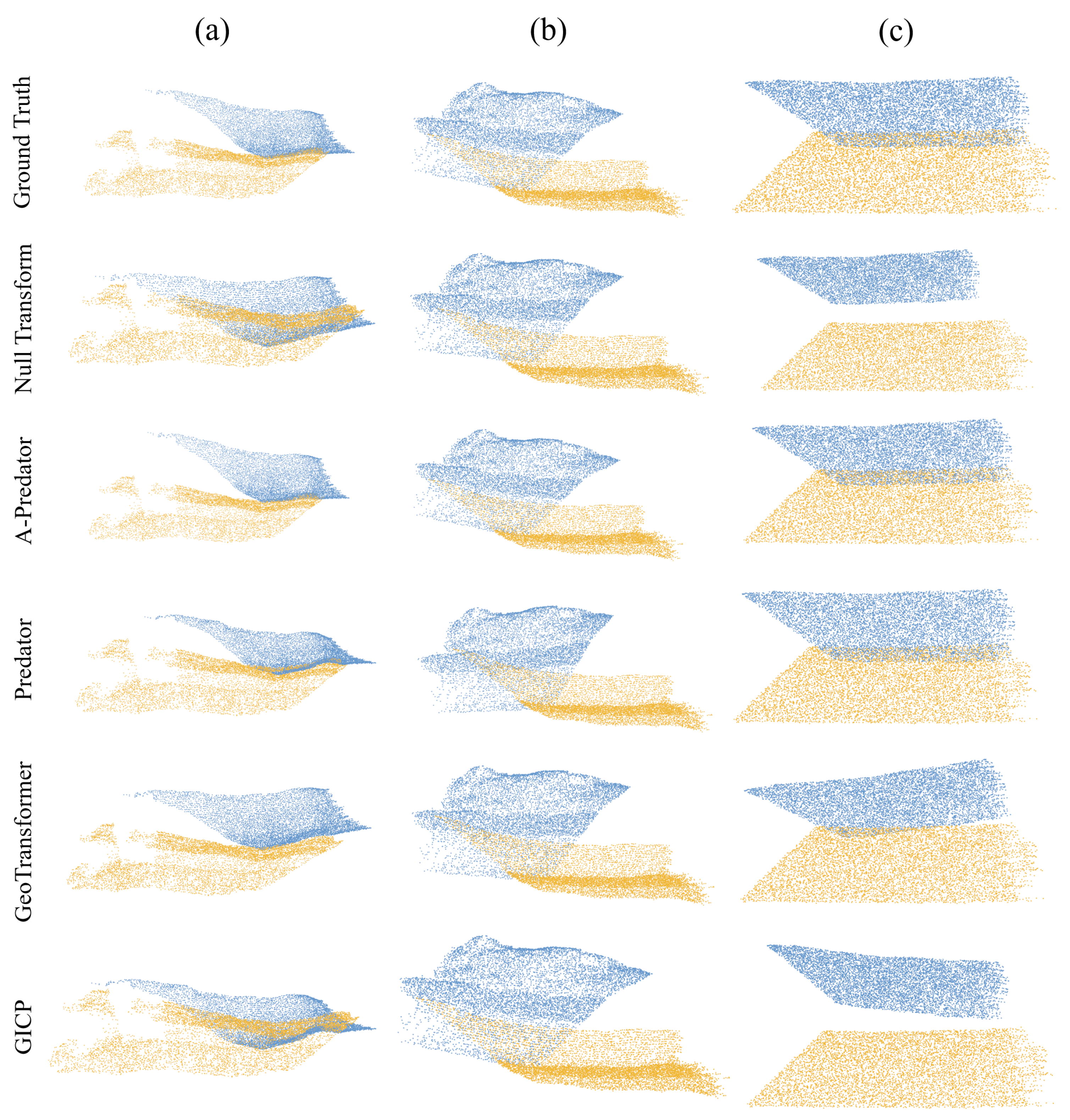
Most existing registration methods for multibeam bathymetry systems rely on Iterative Closest Point (ICP) based algorithms [7,8,9]. These methods are sensitive to initialization and lack robustness in environments with sparse features and severe noise. In recent years, deep learning-based methods have made significant progress in point cloud registration. However, mainstream models (e.g., DCP [10], FCGF [11], DGR [12]) and their core convolution operators (e.g., KPConv [13], DGCNN [14]) are predominantly designed under the assumption that point cloud data is locally isotropic. For instance, KPConv [13] employs a set of kernel points rigidly distributed in space to aggregate information. When applied to MBES point clouds, which have a unique stripe-like structure, this rigid design may fail to capture the underlying geometric priors, resulting in a loss of structural information. Figure 1 presents a visual comparison of registration results produced by different methods on low-overlap MBES submaps.

To address the challenges posed by the strong anisotropy of MBES point clouds, this paper proposes Anisotropic Kernel Point Convolution (A-KPConv), a novel operator whose kernel shape and orientation adaptively align with the local geometric principal directions of the point cloud, enabling more precise extraction of directional structural features. Furthermore, to tackle the low overlap and high noise common in underwater registration, we integrate A-KPConv into Predator [15], an advanced framework for low-overlap registration, constructing A-Predator—a registration model specifically optimized for MBES point clouds. Specifically, we replace the standard KPConv modules in the initial encoder layers of Predator with A-KPConv, enabling structure-aware feature learning in the shallow layers of the network, where geometric information is most explicit. The main contributions of this paper are summarized as follows:

• We design A-KPConv, an anisotropic kernel convolution operator that dynamically adapts the kernel shape and orientation to the local geometric structure, extracting structural features from MBES point clouds more effectively than the isotropic kernels of standard KPConv [13].
• We propose A-Predator, a point cloud registration network optimized for MBES data, which achieves higher accuracy on low-overlap and high-noise inputs by integrating A-KPConv into the encoder’s downsampling blocks.
• We conduct extensive experiments on the public Dotson-east dataset [16] and our self-collected LQL-MBES dataset. The results demonstrate that A-Predator achieves the highest registration recall and consistently low error metrics, particularly in extreme low-overlap scenarios.

2. Related Work

2.1. Point Cloud Neural Network Operators

Research on point cloud neural network operators originated with PointNet [17], which pioneered the direct processing of raw point clouds but was essentially limited by its inability to capture local geometric structures. To circumvent this limitation, PointNet++ [18] and PointNeXt [19] introduced hierarchical feature learning mechanisms; yet, their feature extraction relies excessively on raw Multi-Layer Perceptrons (MLPs), limiting their perception of complex local patterns. To enhance local geometric perception, two mainstream approaches have subsequently emerged. The first involves graph convolution algorithms, represented by DGCNN [14], ECC [20], and AdaptConv [21], which treat point clouds as graph structures and use graph convolution for feature propagation. Nevertheless, these methods are often constrained by the high computational overhead of dynamic graph construction or a lack of flexibility regarding geometric deformation on fixed graph structures. The second approach involves a series of point cloud convolution operators derived from image convolution concepts. These methods [13,22,23,24,25] enhance local geometric perception by designing various types of convolution operators.

In recent years, researchers have begun incorporating Transformers [26] into the field of point cloud processing, leveraging self-attention mechanisms to achieve global modeling of both local and non-local structures. Typical works include PCT [27], the PT series [28], Point-BERT [29], and Point-MAE [30]. However, these methods typically face the issue of computational complexity growing quadratically with the number of points. Although KPConv [13] is not necessarily the optimal point cloud neural network operator, its intuitive, concise and efficient characteristics—inspired by 2D image convolution—have established it as the foundational backbone network for numerous recent point cloud matching architectures [15,31,32,33,34].

2.2. Anisotropic Structure Modeling Methods

With the advancement of deep learning on point clouds, researchers have increasingly recognized that local neighborhood structures exhibit spatial directional preferences, or anisotropy. Consequently, efforts have been made to explicitly incorporate directional modeling into convolution operations to overcome the limitations of traditional isotropic assumptions when processing geometric structures such as strips or thin sheets. For instance, PAI-Conv [35], proposed by Gao et al., employs a set of predefined “kernel points” to generate a soft permutation matrix, which reorders neighborhood points to impose anisotropic filtering. Similarly, DeltaConv [36] by Wiersma et al. approaches the problem from a geometric differential perspective; it introduces operators such as gradient and divergence to construct a scalar-vector dual-stream network, thereby achieving direction-sensitive convolution. Furthermore, Zhang et al. proposed LSPConv [37], which enhances responsiveness to directional variations through anisotropic relative feature encoding and feature weight allocation modules.

Despite their promising performance across various tasks, these methods generally exhibit several limitations: a strong dependency on predefined kernel point layouts; a lack of adaptive alignment based on local principal directions; insufficient integration with mechanisms for convolution kernel deformation or principal direction alignment; and a lack of specialized design for structural priors in extreme anisotropic scenarios, such as the strip-like, highly noisy point clouds generated by multibeam sonar. To address these deficiencies and inspired by these anisotropic modeling works, this paper proposes A-KPConv, specifically tailored for multibeam point clouds. By combining principal direction estimation with a kernel deformation mechanism, A-KPConv achieves adaptive alignment between the convolution kernel and the local structural direction, aiming to enhance feature extraction capabilities on strongly anisotropic point clouds.

It is also worth distinguishing A-KPConv from the deformable variant of KPConv [13], in which each kernel point learns an independent offset directly from the training data. Such learned deformations are entirely task-driven and, in the absence of any geometric prior, can become unreliable when training data are scarce or severely corrupted by noise—both typical of MBES surveys. In contrast, A-KPConv derives the kernel deformation analytically from the local geometry itself, through principal component analysis (PCA)-based principal direction estimation followed by an affine transformation, so that the kernel shape and orientation are explicitly aligned with the underlying strip-like structure before any task-specific learning takes place.

2.3. Underwater Multibeam Point Cloud Registration

The registration of MBES point clouds presents significant challenges due to inherent characteristics such as high noise levels, low density, limited overlap, and strong anisotropy. Existing research primarily follows two paradigms: classical and learning-based approaches. Among classical methods, the deterministic registration framework proposed by Zhao et al. [38] leverages Inertial Measurement Unit (IMU) priors to constrain the rotation search space from three dimensions to one, combining a Branch-and-Bound strategy to enhance both speed and accuracy. Since this framework depends on additional inertial priors rather than the point clouds alone, it is not included in our experimental baselines, which are all evaluated under a unified setting where only the point cloud pair is available. Nevertheless, we view such inertial priors as complementary to point-cloud-only registration, and we discuss their integration as future work (Section 6). Conversely, learning-based methods offer novel perspectives: PointNetKL [39] uses KL divergence minimization to achieve probabilistic registration, demonstrating robustness against noisy data; meanwhile, BathyNN [40] focuses on loop closure detection and coarse registration, using deep features to assist Autonomous Underwater Vehicle (AUV) relocalization.

Nevertheless, these methods remain subject to significant limitations. Classical algorithms often exhibit poor robustness in scenarios characterized by low overlap or large pose deviations. Learning-based methods, on the other hand, are severely hindered by the scarcity of underwater training data and the arduous domain adaptation challenges arising from sonar-specific artifacts, such as stripe patterns and reflection noise. A common limitation is that classical descriptors and existing neural networks do not explicitly account for the strongly anisotropic structures inherent in MBES point clouds, which can hinder robust and discriminative feature extraction. To address this critical issue, we propose A-KPConv. This method aims to enhance local structural representation through the use of adaptive anisotropic convolution kernels, thereby significantly improving matching robustness in challenging underwater environments marked by low overlap and sparse features.

3. Materials and Methods

This section formulates the MBES registration problem (Section 3.1), reviews the Predator baseline architecture (Section 3.2), and details the proposed A-KPConv operator (Section 3.3) and the resulting A-Predator network (Section 3.4).

3.1. Problem Statement

The general objective of 3D point cloud registration is to estimate the optimal rigid transformation $T^{*}$ between two point clouds, P and Q. Let the source point cloud be denoted as $P=\{p_i\in {\mathbb{R}}^3\mid i=1,\dots ,N_p\}$, and the target point cloud as $Q=\{q_j\in {\mathbb{R}}^3\mid j=1,\dots ,N_q\}$. Our task is to seek a rigid transformation $T^{*}=[R^{*}\mid t^{*}]\in SE\left(3\right)$ such that the transformed source point cloud $T\left(P\right)$ achieves maximum alignment with the target point cloud Q within the overlapping region.

However, due to their unique acquisition mechanisms and the inherent characteristics of the underwater environment, the nature of MBES point clouds presents two core challenges to this general task: strong anisotropy with sparse structural features, and inherently low-overlap rates.

We define the objective as:

$$T^{*}=\underset{T\in SE\left(3\right)}{\mathrm{argmin}}d\left(T\left(P\right),Q;\mathcal{F}\right)$$

(1)

where $d(·,·;\mathcal{F})$ denotes a feature-aware registration objective that measures the alignment quality between the transformed source point cloud $T\left(P\right)$ and the target point cloud Q, and $\mathcal{F}$ represents the feature descriptors learned by the model. The overlap rate ${\widehat{P}}_{\mathrm{overlap}}$ between two point clouds is defined as:

$${\widehat{P}}_{\mathrm{overlap}}={\displaystyle \frac{1}{N_p}}{\displaystyle \sum _{i=1}^{N_p}}\mathbb{II}\left(\parallel T_{gt}\left(p_i\right)-NN(T_{gt}\left(p_i\right),Q){\parallel }_2\le ϵ\right)$$

(2)

where $N_p$ denotes the number of source points, $\mathbb{II}(·)$ is the indicator function, and $ϵ$ represents the overlap tolerance threshold. Our method aims to improve registration recall and reduce registration errors under conditions where ${\widehat{P}}_{\mathrm{overlap}}$ is extremely low.

3.2. The Predator Network Architecture

Predator [15] is a widely used 3D point cloud registration network designed for low-overlap point-cloud pairs, making it a relevant baseline for MBES registration. This architecture learns to detect the overlap region between two unaligned point clouds and focuses its sampling of feature points specifically within this area. The architecture comprises three main components: Encoder, Overlap Attention Module, and Decoder.

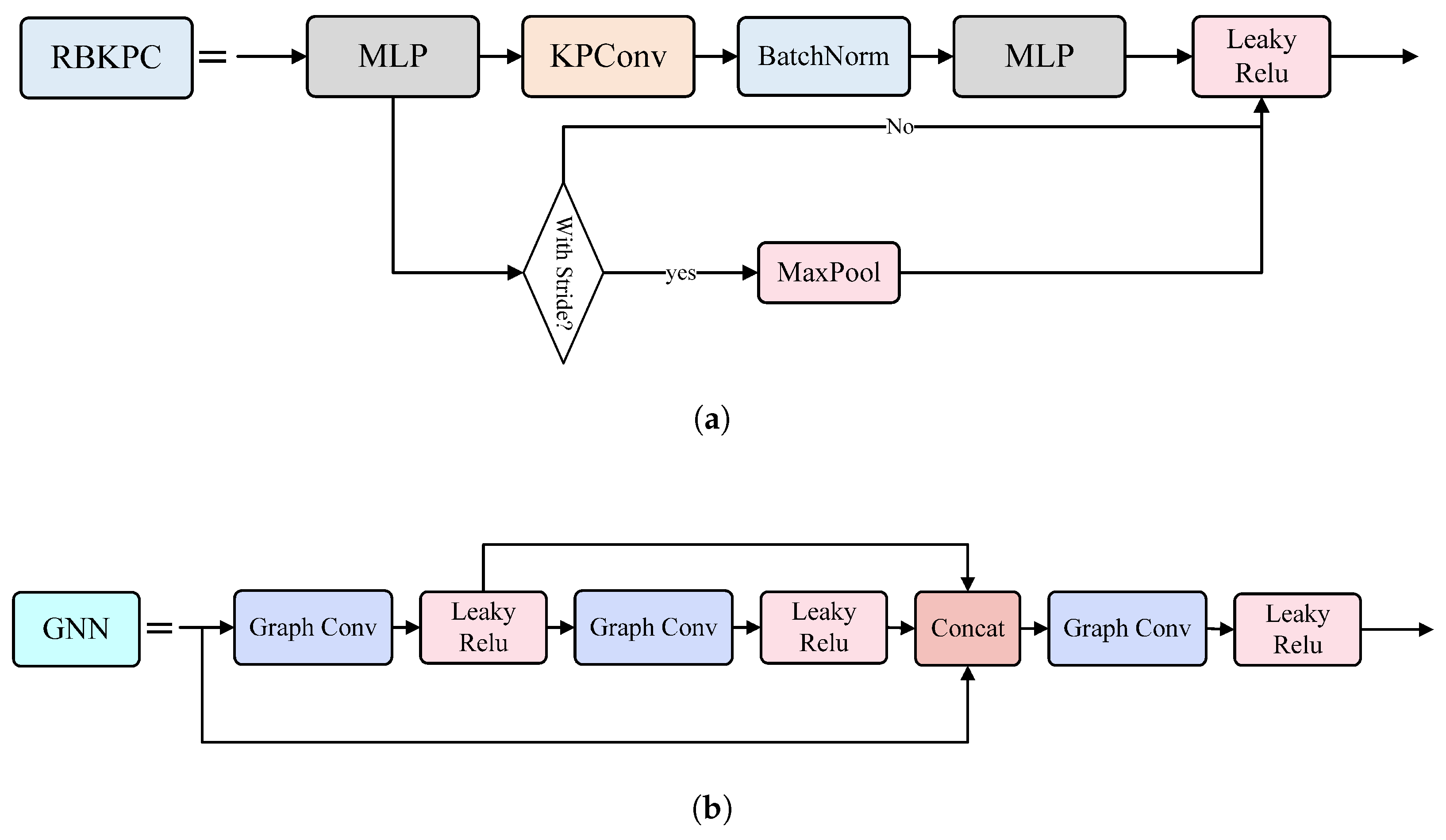
The encoder employs a hybrid of two KPConv [13] blocks—Simple KPConv and ResNet Bottleneck KPConv (RBKPC, Figure 2a)—to extract features from the two input point clouds, thereby generating their respective superpoints.

The core Overlap Attention Module first uses a Graph Neural Network (GNN, Figure 2b) [14] to capture feature neighborhood contexts within each individual point cloud. Subsequently, it employs a multi-head attention mechanism to facilitate information exchange between the superpoints of the two point clouds, enabling the model to determine whether specific superpoints are located within the overlap region. The output point clouds are then processed through another GNN [14] with distinct parameters to verify whether the neighbors of the superpoints lie within the overlap area, thereby performing a final update on the overlap confidence of the superpoints.

This specific design of the Overlap Attention Module ensures that the model maintains a focused local receptive field during intra-cloud information exchange, while using the multi-head attention module to provide a global receptive field for the critical determination of overlap.

Predator [15] employs three distinct loss functions to supervise its three respective outputs—F, o, and m. Specifically, a cross-entropy-based loss is applied to both the overlap scores o and matchability scores m against their ground-truth values. The core component is the Circle Loss [41] applied to feature computation. It performs joint optimization on positive and negative pair similarities; through the dynamic adjustment of gradient balancing factors, it ensures the model learns highly discriminative point cloud feature representations.

$${\mathcal{L}}_{circle}={\displaystyle \frac{1}{K}}{\displaystyle \sum _{i=1}^K}\log \left[1+{\mathcal{E}}_p^{\left(i\right)}·{\mathcal{E}}_n^{\left(i\right)}\right]$$

(3)

where ${\mathcal{E}}_p^{\left(i\right)}$ and ${\mathcal{E}}_n^{\left(i\right)}$ represent the weighted exponential aggregation terms for positive and negative pairs, respectively, defined as:

$$\begin{array}{cc}\hfill {\mathcal{E}}_p^{\left(i\right)}& =\sum _{j\in {\mathcal{P}}^{\left(i\right)}}\exp \left[{\alpha }_p^j(D_{ij}-m_p)\right],\hfill \\ \hfill {\mathcal{E}}_n^{\left(i\right)}& =\sum _{k\in {\mathcal{N}}^{\left(i\right)}}\exp \left[{\alpha }_n^k(m_n-D_{ik})\right]\hfill \end{array}$$

(4)

In Equation (4), $D_{ij}={\parallel {\mathbf{f}}_i-{\mathbf{f}}_j\parallel }_2$ denotes the Euclidean distance between feature vectors in the embedding space. The Circle Loss formulation employs adaptive weighting terms defined as ${\alpha }_p^j=\gamma (D_{ij}-m_p)$ and ${\alpha }_n^k=\gamma (m_n-D_{ik})$, where $\gamma$ serves as the scaling hyperparameter. Regarding the hyperparameters, we adopt the standard relaxation margins of $m_p=0.1$ and $m_n=1.4$ for positive and negative pairs, respectively. Each of the three loss terms is symmetrized by averaging the query-to-gallery and gallery-to-query directions. Following Predator [15], the total objective is their equally weighted sum, ${\mathcal{L}}_{total}={\mathcal{L}}_{circle}+{\mathcal{L}}_{overlap}+{\mathcal{L}}_{matchability}$.

3.3. A-KPConv

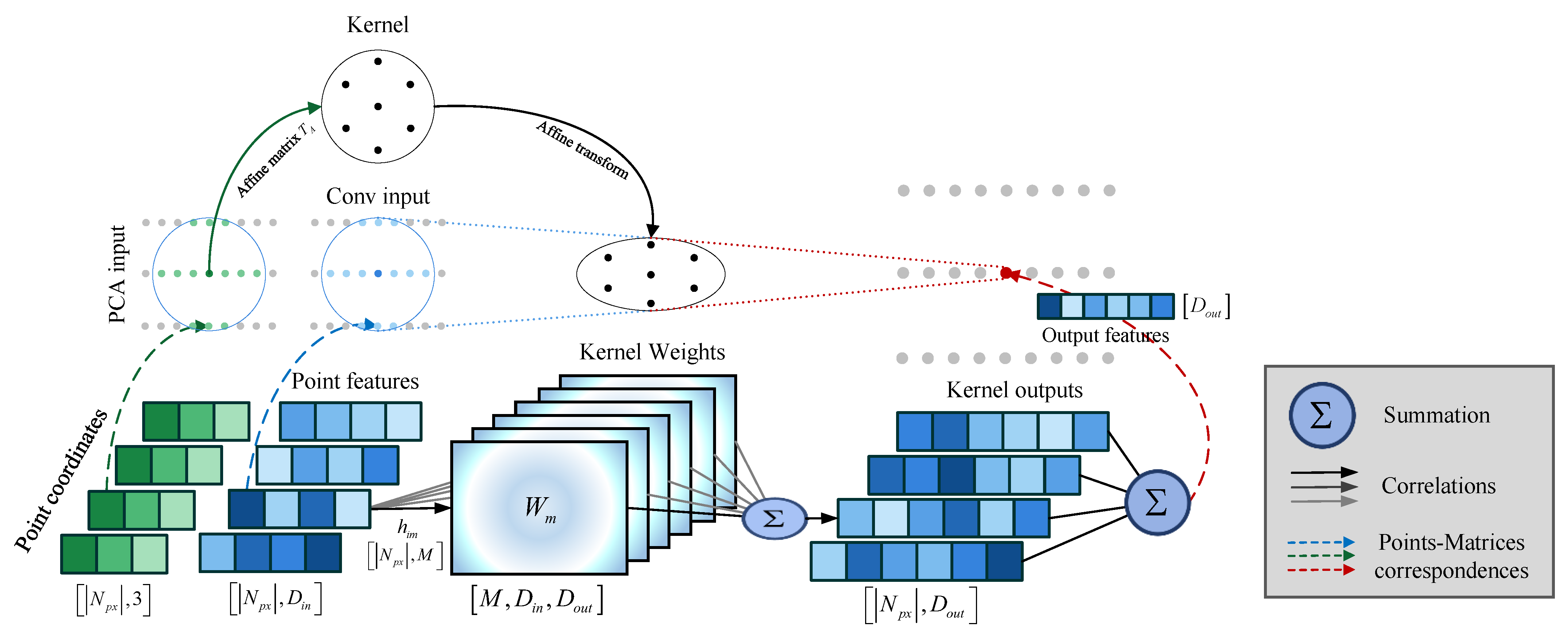
The KPConv [13] module employs kernel points that are isotropically distributed in space to aggregate neighborhood information. However, when confronted with the non-uniform and distinctly anisotropic distribution of MBES point clouds, the feature representation capability of such isotropic kernels is constrained, potentially leading to the learning of erroneous features. To address this challenge, we design A-KPConv, as illustrated in Figure 3. The core philosophy of this operator is to enable the shape and orientation of the convolution kernel to adaptively adjust according to the local geometric features of the point cloud.

Let a point in the point cloud be defined as $x_i\in {\mathbb{R}}^3$, with its corresponding feature denoted as $f_i\in {\mathbb{R}}^D$. For any convolution center point $x_c$, we define its neighborhood for PCA as:

$$N_{px}=\{x_i\in {\mathbb{R}}^3\mid \parallel x_i-x_c{\parallel }_2\le r_p\}$$

(5)

where $r_p$ represents the radius of the PCA scope. In this work, $r_p$ is set equal to the convolution radius of the corresponding KPConv layer, so that the PCA neighborhood coincides exactly with the convolution receptive field and no additional hyperparameter is introduced; a sensitivity analysis of $r_p$ is provided in Section 4.6. To eliminate the influence of position and analyze only the shape of the neighborhood, we translate all neighborhood points such that their centroid is located at the origin:

$$y_i=x_i-\mu$$

(6)

where $\mu ={\displaystyle \frac{1}{|N_{px}|}}{\sum }_{x_i\in N_{px}}{x}_i$ is the centroid of the neighborhood. These centroid-based coordinates are used only for shape analysis. Subsequently, we compute the covariance matrix $C_p$ of the neighborhood point set:

$$C_p={\displaystyle \frac{1}{|N_{px}|}}\sum _{x_i\in N_{px}}{y}_i{y}_i^T$$

(7)

We perform eigendecomposition on $C_p$ to obtain three eigenvectors $(e_1,e_2,e_3)$, representing the first, second, and third principal directions, respectively, along with their corresponding eigenvalues ${\lambda }_1\ge {\lambda }_2\ge {\lambda }_3$. In the implementation, the eigenvalues are clamped to nonnegative values before the scale computation. The eigenvector signs are canonicalized consistently, and the resulting orthonormal basis is adjusted to satisfy $\det \left(R_A\right)=+1$, ensuring that $R_A$ is a proper rotation rather than a reflection. Here, the first principal direction corresponds to the orientation of the strip-like features in MBES data.

Using the PCA results, we construct an affine transformation matrix $T_A\left(x_c\right)$ for each convolution center point $x_c$. This matrix is composed of a rotation matrix $R_A$ and a scaling matrix $S_A$. Specifically, $R_A=[e_1|e_2\left|e_3\right]$ serves to align the coordinate system with the principal directions of the local geometry; meanwhile, $S_A=\mathrm{diag}(s_1,s_2,s_3)$, where $s_j=\sqrt{{\lambda }_j/({\lambda }_2+{\epsilon }_s)}$ for $j\in \{1,2,3\}$ and ${\epsilon }_s$ is a small positive constant for numerical stability ($5\times {10}^{-6}$ in all experiments), is used to perform scaling along the aligned coordinate axes. Finally, the affine transformation matrix for the kernel points is formulated as $T_A\left(x_c\right)=R_A·S_A$.

Note that the scale along the first principal direction, $s_1=\sqrt{{\lambda }_1/({\lambda }_2+{\epsilon }_s)}$, may become large in nearly degenerate neighborhoods where ${\lambda }_2\to 0$. Several properties mitigate this behavior in practice. First, the scaling is self-normalized by the second principal variance, so that neither $s_2$ nor $s_3$ exceeds 1, while the growth of $s_1$ follows the square root of the anisotropy ratio. Second, ${\epsilon }_s$ prevents singular division, and the nonnegative eigenvalue clamp avoids invalid square-root operations caused by small numerical round-off errors. Finally, the correlation in Equation (9) is truncated at distance $\sigma$ with $h\in [0,1]$, so an over-stretched kernel point loses its influence on neighboring points rather than producing an unbounded aggregation weight. Training remained numerically stable in all our experiments. Nevertheless, no explicit fallback is used for nearly degenerate neighborhoods; under extreme sparsity or weak local structure, the estimated eigen-directions may still become unstable and the aggregation may lose informative kernel-point responses. We therefore treat such neighborhoods as a limitation rather than claiming unconditional numerical robustness.

In the standard KPConv [13], the convolution kernel comprises a set of base kernel points $\{k_m\mid 1\le m\le M\}$ defined in a local coordinate frame anchored at the convolution center. In contrast, within A-KPConv, these base kernel points undergo dynamic deformation via the transformation matrix $T_A\left(x_c\right)$, yielding a set of anisotropic kernel points $\left\{k_{am}^{\prime }\left(x_c\right)\right\}=\{T_A\left(x_c\right)·k_m\}$ that adapt to the local geometry and remain anchored at $x_c$. Since the eigen-directions and eigenvalues used to construct $T_A\left(x_c\right)$ are translation-invariant properties of the neighborhood shape, the transformation estimated in the centroid frame can be applied directly in this center-anchored frame. Following the KPConv convention, the influence weights and the feature aggregation are computed in the center-relative coordinates of the neighbor points. The aggregated features can be expressed as:

$${\mathcal{F}}_{A\text{-}KP}\left(x_c\right)=\sum _{x_i\in N_{px}}{\displaystyle \sum _{m=1}^M}h\left(z_i,k_{am}^{\prime }\left(x_c\right)\right)W_m{f}_i$$

(8)

where $W_m$ denotes the learnable weight matrix associated with the m-th kernel point, $z_i=x_i-x_c$ is the center-relative position of the neighbor point $x_i$, and $h(·)$ denotes the correlation between the kernel point $k_{am}^{\prime }\left(x_c\right)$ and $z_i$:

$$h\left(z_i,k_{am}^{\prime }\left(x_c\right)\right)=\max \left(0,1-{\displaystyle \frac{\parallel z_i-k_{am}^{\prime }\left(x_c\right){\parallel }_2}{\sigma }}\right)$$

(9)

where $\sigma$ represents the influence radius of the kernel.

3.4. A-Predator Architecture

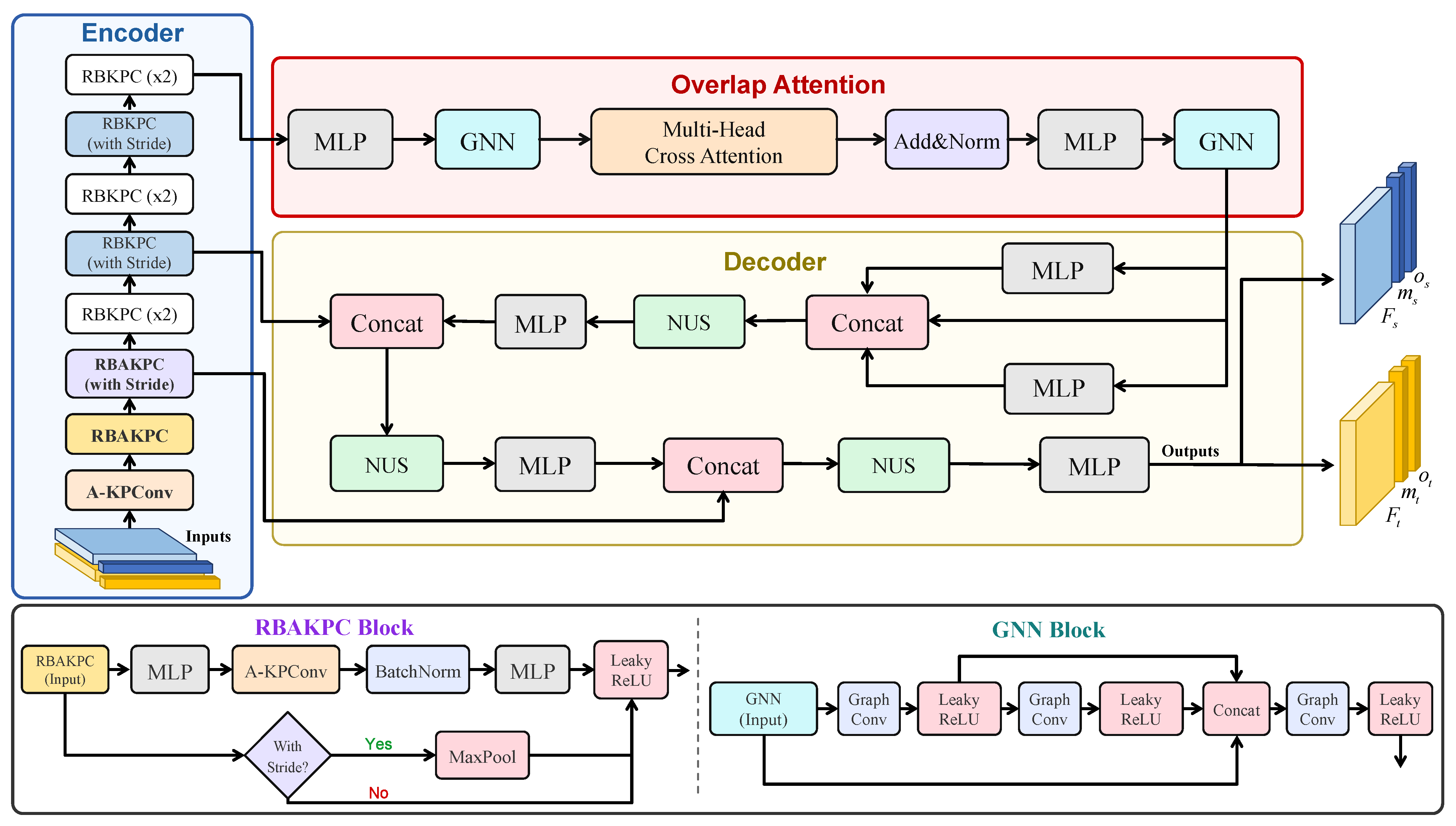
Figure 4 illustrates the overall architecture of the improved A-Predator. While our model inherits the general encoder-decoder structure of Predator [15], the core modifications are concentrated within the encoder section. In the initial stages of the network, where geometric structural information is most explicit, the deployment of the structure-aware A-KPConv is most effective for capturing anisotropic features. Conversely, as the network deepens and representations become increasingly abstract, the standard isotropic KPConv [13] is sufficient for feature extraction from high-level features, where the benefit of directional modeling diminishes (cf. the replacement-depth ablation in Section 4.3).

Consequently, we replace the standard KPConv [13] modules in the first three layers of the Predator encoder with our proposed A-KPConv layers. The first layer applies a Simple A-KPConv block for initial structure-aware feature extraction at the full input resolution. The second and third layers use ResNet Bottleneck A-KPConv (RBAKPC) blocks, which incorporate residual connections around the anisotropic convolution to facilitate gradient flow while preserving the ability to capture directional geometric features; the third block operates with stride and performs the first downsampling in the encoder. Within each RBAKPC block, the internal KPConv modules are replaced with A-KPConv, while the residual pathway and strided convolution for downsampling remain unchanged. Deeper encoder layers retain the original isotropic KPConv.

To ensure a fair evaluation, both the network’s bottleneck layer—specifically the Overlap Attention Module with its GNN-based intra-cloud message passing and cross-attention mechanism—and the subsequent decoder remain identical to those in the original Predator [15], isolating the effect of the anisotropic convolution replacement so that performance differences can be attributed directly to the structure-aware feature learning in the encoder.

4. Results

The experiments are organized into six parts: evaluation on the public Dotson-east multibeam point cloud dataset [16] (Section 4.1), testing on our self-collected LiQuan Lake (LQL) MBES dataset (Section 4.2), ablation studies on anisotropic convolution operators and architecture-level design choices (Section 4.3), a cross-dataset generalization analysis against three baseline models (Section 4.4), a computational efficiency analysis (Section 4.5), and a sensitivity analysis of the PCA neighborhood radius (Section 4.6). All experiments are conducted on a system configured with an Intel(R) Xeon(R) Platinum 8255C CPU @ 2.50 GHz, 24 GB of RAM, and an NVIDIA GeForce RTX 3090 GPU, running 64-bit Ubuntu 20.04 with CUDA 11.3 and the PyTorch 1.9.1 framework.

We evaluated our proposed A-Predator model against state-of-the-art (SOTA) deep learning-based registration models and traditional algorithms. The evaluation metrics included Registration Recall (RR), Relative Translation Error (RTE), and Relative Rotation Error (RRE). The comparative methods selected are as follows:

• Predator [15]: A learning-based keypoint descriptor designed for low-overlap point cloud registration, which serves as the foundational framework for our algorithm.
• GeoTransformer [32]: A transformer-based framework that employs a coarse-to-fine strategy to achieve accurate registration in low-overlap scenarios.
• Fully Convolutional Geometric Features (FCGF) [11]: The pioneering fully convolutional point cloud feature extractor.
• Deep Global Registration (DGR) [12]: A learning-based method for robust outlier rejection.
• BathyNN [40]: A learning-based architecture specifically designed for loop closure detection in multibeam point clouds.
• Generalized Iterative Closest Point (GICP) [9]: A classic geometric algorithm that has demonstrated significant advantages in underwater point cloud registration.
• Fast Point Feature Histograms (FPFH) [42]: A widely used handcrafted point cloud feature descriptor.

For a fair comparison, all learning-based methods (Predator, GeoTransformer, FCGF, and DGR) were fine-tuned on the Dotson-east training set using the same data augmentation strategy before evaluation on the corresponding test set. BathyNN was also retrained following the same protocol to serve as a reference baseline. For feature-based methods, predicted transformations were estimated using the RANdom SAmple Consensus (RANSAC) algorithm [43] (50000 iterations; 3-point sampling for FPFH [42] and 4-point sampling for learning-based descriptors). For each dataset, the test pairs, sampled transformations, noise realizations, and crop masks were generated with fixed random seeds and reused unchanged across all compared methods. For both datasets, RR is defined as follows: a pair of submaps is considered successfully recalled if the estimated transformation matrix satisfies both $RRE\le 5^{\circ }$ and $RTE\le 10\mathrm{m}$.

4.1. Experiments on Public Datasets

The Dotson-east dataset employed for testing is derived from the work of [16]. This is an MBES registration dataset constructed from Autonomous Underwater Vehicle (AUV) missions in the West Antarctic. The original researchers configured each submap to comprise 100 consecutive sonar pings, with a step size of 20 pings. Consequently, an 80% data overlap exists between two consecutive submaps. This process yielded a total of 9415 submaps, which were further partitioned into training, validation, and testing sets containing 7263, 1206, and 946 submaps, respectively. Pairing each submap with offsets of zero to four submaps yielded nominal overlap rates of 100%, 80%, 60%, 40%, and 20%, respectively. This construction produced approximately 36,300, 6015, and 4715 submap pairs for training, validation, and testing, respectively.

During the training and testing phases, submap pairs for registration are synthesized by applying rotation, translation, noise addition, and random cropping to individual submaps. To simulate heading error during sonar data acquisition, we restricted rotation transformations to the Z-axis, with rotation angles sampled within the range of $[0^{\circ },{10}^{\circ }]$; rotations about the X and Y axes were not applied. Regarding translation, we sampled within the range of $[-40,40]$ m along the X and Y axes, and within $[-2,2]$ m along the Z-axis. Furthermore, to enhance model robustness and increase the challenge of the testing scenarios, jitter noise was added to each submap during data preprocessing, accompanied by an independent 70% crop in the XY plane. This implies that the effective overlap of the cropped submap pairs is reduced to approximately half of the original value. For instance, a submap pair with an initial overlap of 20% would possess an effective overlap of 10% post-cropping.

Although the low-overlap pairs are synthesized via geometric transformations and cropping, this simulation strategy is designed to mirror the dominant factors encountered in real-world MBES registration. The Z-axis rotation reproduces heading drift, which is the predominant pose deviation for underwater vehicles, since roll and pitch are effectively stabilized by the platform; the translations along the X and Y axes emulate horizontal positioning drift, whereas the small-range Z-axis translation reflects the comparatively stable depth keeping of the vehicle. The jitter noise mimics sonar measurement errors arising from water-column fluctuations, and the random cropping reproduces the reduced overlap induced by trajectory deviations and variations in survey coverage. Moreover, because both datasets are constructed from real MBES surveys, practical effects such as sonar noise, seafloor variability, and density inconsistencies are inherently preserved within the submaps themselves rather than being synthesized away. In addition, residual motion distortion induced by platform movement (e.g., INS drift) is inherently preserved, as each submap is stacked from real consecutive sonar pings rather than synthesized. We also note that, in extreme cases, random cropping may remove the already limited overlapping region entirely, making such a pair intrinsically unregistrable; since this affects all compared methods equally, it does not compromise the fairness of the evaluation (see Section 5.5).

As shown in

Table 1. Quantitative results on the Dotson-east dataset with varying effective overlap ratios. Recall indicates the percentage of pairs with $RRE\le 5^{\circ }$ and $RTE\le 10\mathrm{m}$. RRE and RTE are averaged only over successfully recalled pairs. Bold values highlight the proposed method. The ‘–’ symbol indicates that no pairs were successfully recalled under the corresponding condition.

Method	Effective Overlap Ratio
	0.10			0.20			0.30			0.40			0.50
	Rec.	RTE	RRE	Rec.	RTE	RRE	Rec.	RTE	RRE	Rec.	RTE	RRE	Rec.	RTE	RRE
FPFH	0.11	2.4640	4.4363	0.53	3.7980	3.2575	4.03	3.4350	2.6124	9.10	3.1250	2.5046	22.41	3.0230	2.1492
BathyNN	0.43	5.5930	3.8440	3.50	4.2940	2.8342	11.55	3.1230	2.4704	21.70	2.9550	2.0795	73.04	1.6890	1.4391
DGR	–	–	–	0.32	1.7640	0.8798	18.75	1.1670	0.4925	51.32	0.9900	0.4999	80.44	0.4642	0.2660
GICP	45.01	1.1080	1.1201	58.43	0.5621	0.3400	67.80	0.3959	0.2173	70.90	0.2535	0.1344	72.73	0.1658	0.0856
FCGF	2.44	2.9240	2.7115	44.64	2.8440	2.0628	74.57	2.6860	1.6986	89.21	2.6330	1.5790	98.62	1.0590	0.6124
GeoTrans	–	–	–	54.33	0.6772	0.5913	87.97	0.4846	0.3832	92.31	0.3863	0.2781	99.88	0.3157	0.2002
Predator	31.63	4.1040	2.5856	63.64	3.4280	2.1664	81.25	3.3570	1.8174	88.57	2.7170	1.3662	100.00	1.0850	0.5408
Ours	59.55	1.0110	0.7099	86.32	0.6364	0.3741	97.25	0.4002	0.2242	99.79	0.2638	0.1381	100.00	0.1619	0.0934

Rec.: Recall (%); RTE: Relative Translation Error (m); RRE: Relative Rotation Error (°). The gray background highlights the proposed method.

, A-Predator achieves the highest recall across all evaluated overlap settings and maintains consistently low translation and rotation errors, especially under low-overlap conditions.

4.2. Experiments on Self-Collected Dataset

This section presents registration experiments on our self-collected LQL-MBES dataset, covering the experimental site, acquisition platform, data processing pipeline, and dataset composition, to demonstrate the transferability of A-Predator across diverse scenarios and various models of multibeam sonar systems.

4.2.1. Experimental Setup and Data Preparation

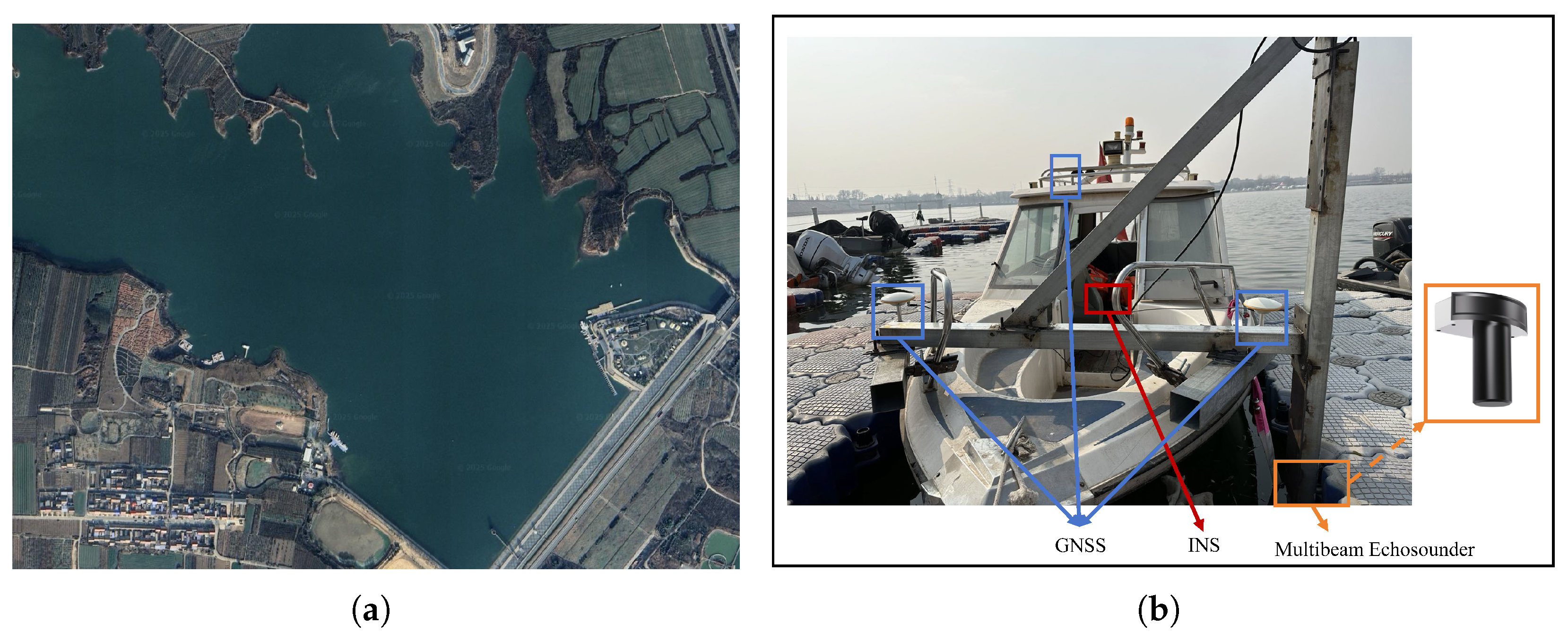
The experiments use the HDY-BD400D MBES (Whale Wave Technology Inc., Kunming, China); its key performance specifications are detailed in

Table 2. HDY-BD400D MBES main performance specifications.

Parameters	Metrics
Operating frequency	$400\mathrm{kHz}$–$700\mathrm{kHz}$, real-time continuously adjustable with a step size of $1\mathrm{kHz}$
Cross-track beam width	$1^{\circ }$@$400\mathrm{kHz}$; ${0.5}^{\circ }$@$700\mathrm{kHz}$
Along-track beam width	$1^{\circ }$@$400\mathrm{kHz}$; ${0.5}^{\circ }$@$700\mathrm{kHz}$
Number of beams	$256/512$ (Equal angle/equal distance)
Sector opening angle	10–180° real-time continuously adjustable
Range	$200\mathrm{m}$ @ $400\mathrm{kHz}$
Pulse width	$10\mathsf{\mu }s$–$800\mathsf{\mu }s$
Ping rate	Up to $50\mathrm{Hz}$

. The experimental site and the configuration of the data acquisition platform are illustrated in Figure 5. Notably, the experimental site is a shallow-water environment with a mean depth of approximately 4 m. At this depth, the MBES produces a swath width of merely 6–8 m, which, combined with the 256-beam configuration, yields a high point density within each ping and a pronounced, regular stripe-like pattern. These acquisition characteristics underlie the generally strong registration performance on this dataset, as further analyzed in Section 5.2.

We collected data from 16 distinct patches across various underwater scenarios within the region illustrated in Figure 5.

Within each patch, each submap was configured to comprise 200 consecutive sonar pings, with a step size of 50 pings. Consequently, adjacent submaps have a nominal overlap rate of 75%, yielding 250 submaps per patch and 4000 submaps in total. The 16 complete patches were partitioned into 12 training, 2 validation, and 2 testing patches (0.75:0.125:0.125); no submap pair was constructed across patch boundaries, thereby preventing highly overlapping submaps from leaking between subsets. Within each patch, offsets of zero to three submaps yielded nominal overlap rates of 100%, 75%, 50%, and 25%, respectively. This construction produced approximately 11,990, 1990, and 1990 submap pairs for training, validation, and testing, respectively. During the training and testing phases, we adopted the same transformation strategy employed for the Dotson-east dataset [16], incorporating corresponding levels of noise jitter and random cropping.

4.2.2. Experiment Results on the LQL-MBES Dataset

During the testing phase, the same 70% XY crop (Section 4.1) reduces the nominal overlap rates of 25%, 50%, 75%, and 100% to the effective values of 12.5%, 25%, 37.5%, and 50%, respectively. Furthermore, a single global scale factor was applied uniformly to all LQL-MBES point clouds to align their overall spatial scale with the Dotson-east data [16]. All transformations, success thresholds, and RTE values for LQL-MBES were evaluated in this rescaled metric coordinate system; accordingly, the reported translation errors refer to the rescaled rather than the original acquisition coordinates. As shown in

Table 3. Quantitative results on the LQL-MBES dataset with varying effective overlap ratios. Recall indicates the percentage of pairs with $RRE\le 5^{\circ }$ and $RTE\le 10\mathrm{m}$ in the rescaled metric coordinate system. RRE and RTE are averaged only over successfully recalled pairs. Bold values highlight the proposed method. The ‘–’ symbol indicates that no pairs were successfully recalled under the corresponding condition.

Method	Effective Overlap Ratio
	0.125			0.25			0.375			0.50
	Rec.	RTE	RRE	Rec.	RTE	RRE	Rec.	RTE	RRE	Rec.	RTE	RRE
FPFH	–	–	–	–	–	–	2.41	4.7510	2.5859	5.41	4.6650	2.4548
BathyNN	0.41	8.0660	2.1296	0.61	3.7230	3.4151	3.83	3.8940	2.2753	11.42	2.3330	2.2784
DGR	–	–	–	0.20	1.2320	0.4957	75.46	0.4810	0.2246	96.99	0.2205	0.0936
GICP	10.76	1.2480	0.4235	11.71	1.4800	0.5242	12.88	0.9014	0.3141	17.63	0.4398	0.1370
FCGF	9.01	0.2997	0.2138	34.14	0.3187	0.1977	91.14	0.8983	0.8135	100.00	0.5012	0.4147
GeoTrans	57.39	1.6652	1.7575	76.01	1.3296	1.3880	80.61	1.2345	1.2336	85.20	1.0962	1.0936
Predator	88.86	0.6431	0.9026	96.58	0.5313	0.5425	100.00	0.2938	0.2451	100.00	0.2030	0.1842
Ours	91.89	0.3536	0.2748	98.18	0.3868	0.2521	100.00	0.2586	0.1383	100.00	0.2083	0.1360

Rec.: Recall (%); RTE: Relative Translation Error (m); RRE: Relative Rotation Error (°). The gray background highlights the proposed method.

, A-Predator achieves the highest recall among the evaluated methods on LQL-MBES, exceeding 90% at every evaluated overlap level while maintaining competitive translation and rotation errors. Compared with Predator [15] at 12.5% overlap, the RTE decreases from 0.6431 m to 0.3536 m and the RRE from ${0.9026}^{\circ }$ to ${0.2748}^{\circ }$ in the rescaled metric coordinate system.

4.3. Ablation Study on Anisotropic Convolution Modules

To validate the effectiveness and necessity of our proposed A-KPConv for MBES data, we conduct an ablation study comparing various anisotropic convolution operators. We replace the A-KPConv layers in the A-Predator encoder with two other state-of-the-art anisotropic operators discussed in Section 2.2: PAI-Conv [35] and LSPConv [37]. DeltaConv [36], also reviewed in Section 2.2, is not included: its anisotropy stems from a coupled scalar–vector dual-stream architecture rather than a single convolution operator, precluding a layer-level controlled comparison. All variants are tested on both the Dotson-east and LQL-MBES datasets across varying effective overlap ratios, with a particular focus on highly challenging low-overlap conditions (e.g., 10% and 12.5%).

We establish the following network variants for comparison:

• Baseline (Predator): The original Predator [15] using standard isotropic KPConv in all encoder layers.
• PAI-Predator: Replaces the first three encoder layers with PAI-Conv [35].
• LSP-Predator: Replaces the first three encoder layers with LSPConv [37].
• A-Predator (Ours): Our proposed method replacing the first three encoder layers with A-KPConv.

The registration results of these operator-level variants on both datasets are summarized in

Table 4. Ablation study results comparing different anisotropic convolution operators across two datasets (Dotson-east and LQL-MBES) under varying effective overlap ratios. RTE and RRE are averaged only over successfully recalled pairs; LQL-MBES RTE values use the rescaled metric coordinate system described in Section 4.2. Bold values highlight the proposed method.

Dataset	Method	Effective Overlap Ratio
		0.10			0.20			0.30			0.40
		Rec.	RTE (m)	RRE (°)	Rec.	RTE (m)	RRE (°)	Rec.	RTE (m)	RRE (°)	Rec.	RTE (m)	RRE (°)
		(%)	Mean	Mean	(%)	Mean	Mean	(%)	Mean	Mean	(%)	Mean	Mean
Dotson -east	Predator	31.63	4.1040	2.5856	63.64	3.4280	2.1664	81.25	3.3570	1.8174	88.57	2.7170	1.3662
	PAI-Predator	40.50	3.5117	2.0034	68.10	2.8212	1.7638	85.40	2.4765	0.7541	91.20	1.8936	1.0039
	LSP-Predator	39.70	3.8323	2.3547	69.50	2.5361	1.3354	92.10	1.0038	0.6782	98.79	0.3495	0.3216
	A-Predator (Ours)	59.55	1.0110	0.7099	86.32	0.6364	0.3741	97.25	0.4002	0.2242	99.79	0.2638	0.1381
		0.125			0.25			0.375			0.5
LQL -MBES	Predator	88.86	0.6431	0.9026	96.58	0.5313	0.5425	100.00	0.2938	0.2451	100.00	0.2030	0.1842
	PAI-Predator	89.00	0.5824	0.7496	97.10	0.5031	0.4937	100.00	0.2842	0.2008	100.00	0.2135	0.1793
	LSP-Predator	89.04	0.5778	0.7632	97.60	0.4306	0.3959	100.00	0.2604	0.1697	100.00	0.2041	0.1385
	A-Predator (Ours)	91.89	0.3536	0.2748	98.18	0.3868	0.2521	100.00	0.2586	0.1383	100.00	0.2083	0.1360

.

Beyond the operator-level comparison above, we further examine two architecture-level design choices of A-Predator on the Dotson-east dataset: how many encoder blocks should be replaced, and whether the analytic PCA-based deformation can be substituted by kernel-point offsets learned from data. We train four additional variants: Ak-Predator replaces only the first k encoder blocks with A-KPConv ($k\in \{1,2,4\}$), while Deformable-Predator replaces the first three encoder blocks with deformable KPConv [13]. All variants are trained and evaluated under the same protocol as the operator-level ablation above, and the results are summarized in

Table 5. Ablation of the replacement depth and the deformation mechanism on the Dotson-east dataset. Ak-Predator replaces the first k encoder blocks with A-KPConv; Deformable-Predator replaces the first three blocks with deformable KPConv. Recall is reported at effective overlap ratios of 0.10–0.40; RTE and RRE are reported at the most challenging 0.10 overlap. Bold values highlight the proposed method.

Method	Rec. (%)				RTE (m)	RRE (°)
	0.10	0.20	0.30	0.40
Predator	31.63	63.64	81.25	88.57	4.1040	2.5856
A1-Predator	44.50	73.50	88.80	94.00	2.7200	1.7000
A2-Predator	52.80	80.30	93.60	97.50	1.5900	1.0600
A3-Predator (Ours)	59.55	86.32	97.25	99.79	1.0110	0.7099
A4-Predator	59.20	86.55	97.10	99.85	1.0350	0.6950
Deformable-Predator	47.80	76.20	91.50	96.80	2.1800	1.3900

. For Deformable-Predator, the fitting and repulsive regularization terms of deformable KPConv [13] were retained, and all variants were assigned the same optimization budget.

Two observations follow. First, the observed benefit of A-KPConv grows monotonically with the replacement depth up to three blocks—the recall at 10% overlap rises from 44.50% (A1-Predator) to 52.80% (A2-Predator) and 59.55% (A3-Predator)—and then plateaus in this ablation: replacing the fourth block changes the recall by no more than 0.4 percentage points with mixed signs, while still increasing the forward latency (from 64 ms to 66 ms, measured under the protocol of Section 4.5). This supports the architectural rationale in Section 3.4: within the evaluated setting, replacing the first three encoder blocks provides the best accuracy–cost trade-off. Second, although Deformable-Predator improves over the isotropic baseline, it remains below A3-Predator under low overlap (47.80% vs. 59.55% recall at 10% overlap, with both error metrics roughly doubled), despite introducing approximately 44 k additional learnable parameters and 12.5% more FLOPs (20.09 vs. 17.86 GFLOPs). Under the matched training budget and official deformable-KPConv regularization, these results suggest that explicit PCA-based geometric alignment is an important contributor to the observed gain in this MBES setting.

4.4. Evaluation of Cross-Dataset Transfer

This section evaluates how the compared models transfer from Dotson-east to a distinct MBES target dataset. We directly evaluate the models trained on Dotson-east [16]—without any fine-tuning—on the globally rescaled LQL-MBES test set.

The data presented in

Table 6. Cross-dataset transfer comparison on the globally rescaled LQL-MBES dataset without fine-tuning. RRE and RTE are averaged only over successfully recalled pairs, and RTE uses the rescaled metric coordinate system.

Method	Overlap	Rec. (%)	RTE (m)	RRE (°)
GeoTransformer	0.125	8.90	0.5971	0.5071
	0.25	43.60	1.9600	1.9300
	0.375	77.90	1.5200	1.4800
	0.5	84.80	1.3100	1.2600
Predator	0.125	23.68	1.2940	1.7065
	0.25	51.41	1.1150	1.2241
	0.375	95.98	0.5209	0.5019
	0.5	99.00	0.3105	0.2750
LSP-Predator	0.125	28.90	1.1900	1.4800
	0.25	56.80	0.8800	0.8600
	0.375	97.00	0.4300	0.3500
	0.5	99.20	0.2700	0.2100
A-Predator (Ours)	0.125	37.25	0.4606	0.3312
	0.25	63.91	0.4138	0.2714
	0.375	98.19	0.3444	0.2113
	0.5	99.40	0.2382	0.1515

provide evidence that A-Predator transfers more effectively than Predator [15], LSP-Predator [37], and GeoTransformer [32] from Dotson-east to the globally rescaled LQL-MBES target without fine-tuning. GeoTransformer has 8.90% recall at 12.5% overlap; its error metrics at this level are averaged over the few successful pairs only and are therefore not directly comparable with errors computed on a broader successful subset. LSP-Predator transfers better than Predator but remains below A-Predator at every evaluated overlap level, most notably under low-overlap conditions (28.90% vs. 37.25% recall at 12.5% overlap). Broader generalization across acquisition conditions remains to be evaluated.

4.5. Computational Efficiency

To quantify the practical overhead introduced by the PCA-based anisotropic adaptation, we profile the per-pair inference latency of all compared methods on the Dotson-east test set [16]. All measurements are conducted on the hardware platform described at the beginning of Section 4, with FP32 precision, a batch size of one, and at most 10 k points per cloud. Timings are collected as sequential per-pair latencies (num_workers = 1, i.e., without deliberate CPU–GPU pipelining) over 1000 test pairs per overlap setting, after 50 warm-up runs.

Table 7. Per-pair end-to-end inference latency of all compared methods on the Dotson-east test set, averaged over 1000 pairs per overlap setting after 50 warm-up runs. Latency includes preprocessing, feature extraction, matching, and pose estimation. All learning-based methods estimate the pose with RANSAC (50 k iterations, 4-point sampling), except FPFH (3-point sampling); GICP performs iterative geometric optimization without correspondences. The 95% interval is approximated from the observed timing range.

Method	Latency (s), Mean ± Std	95% Interval (s)	Throughput (Pairs/s)
GICP	0.22 ± 0.07	0.08–0.36	4.5
FPFH + RANSAC	0.34 ± 0.07	0.21–0.47	2.9
FCGF + RANSAC	0.25 ± 0.04	0.17–0.33	4.0
DGR	0.25 ± 0.05	0.15–0.35	4.0
BathyNN + RANSAC	0.36 ± 0.07	0.23–0.49	2.8
GeoTransformer + RANSAC	0.38 ± 0.06	0.26–0.50	2.6
Predator + RANSAC	0.39 ± 0.06	0.28–0.50	2.6
PAI-Predator + RANSAC	0.41 ± 0.06	0.29–0.53	2.4
LSP-Predator + RANSAC	0.43 ± 0.07	0.30–0.56	2.3
A-Predator (Ours) + RANSAC	0.42 ± 0.06	0.30–0.54	2.4

reports the end-to-end latency and throughput of all methods. A-Predator attains a mean latency of 0.42 s per pair (2.4 pairs/s), only 7.7% slower than the Predator baseline (0.39 s), and remains slightly faster than LSP-Predator. GICP and FCGF are the fastest, benefiting from their correspondence-free optimization and lightweight sparse-convolution designs, respectively. Overall, all learning-based methods sustain throughputs above 2 pairs/s, which is adequate for near-real-time processing of MBES survey data.

Table 8. Computational cost breakdown of Predator and A-Predator. FLOPs, latency, and memory are reported as mean ± std over the Dotson-east test pairs. A-KPConv adds no learnable parameters and negligible FLOPs; the +30 ms forward overhead is concentrated in the first three encoder blocks and is memory- and latency-bound.

Metric	Predator	A-Predator (Ours)	Overhead
Trainable parameters (M)	7.4249	7.4249	0
FLOPs per pair (G)	17.80 ± 3.5	17.86 ± 3.5	≈0.06
Network forward (ms)	34 ± 6	64 ± 11	+30 ± 8
End-to-end latency (ms)	390 ± 56	420 ± 61	+30 ± 8
Peak GPU memory (GB)	2.45 ± 0.23	2.56 ± 0.25	+0.11 ± 0.05

further isolates the cost of A-KPConv. Since the per-neighborhood PCA operates only on $3\times 3$ covariance matrices, A-KPConv introduces no additional learnable parameters (7.4249 M for both models) and increases the FLOPs per pair by merely about 0.3% (17.80 vs. 17.86 GFLOPs). The overhead is therefore memory- and latency-bound rather than compute-bound: the network forward pass grows from 34 ms to 64 ms (≈+88%), yet even after this increase the forward pass accounts for only ≈15% of the 420 ms end-to-end latency of A-Predator (about 9% for the 390 ms baseline). The pipeline is dominated by CPU-side preprocessing and neighborhood indexing (190 ms, ≈49% of the baseline latency) and RANSAC pose estimation (143 ms, ≈37%). Within the additional 30 ms, the batched $3\times 3$ eigendecomposition (torch.linalg.eigh) is the clear bottleneck ($\approx 11$ ms); the remainder arises from neighbor gathering, covariance computation, the kernel-point affine transformation, and associated temporary tensors and synchronization. Peak GPU memory increases by 0.11 GB ($\approx 4.5\%$), mainly from storing per-center deformed kernel points and intermediate PCA tensors in the first three encoder blocks.

4.6. Sensitivity of the PCA Neighborhood Radius

The PCA neighborhood radius $r_p$ (Equation (5)) controls how large a region contributes to the principal direction estimation. To assess its impact, we retrain A-Predator on Dotson-east with the radius of every replaced block scaled uniformly by a factor $\gamma \in \{0.5,1.5,2.0\}$ relative to the default ($\gamma =1.0$, i.e., $r_p$ equal to the per-layer convolution radius), keeping the training and evaluation protocol identical. The results are summarized in

Table 9. Sensitivity of A-Predator to the PCA neighborhood radius on the Dotson-east dataset. The radius of every replaced block is scaled uniformly by $\gamma$ relative to the per-layer convolution radius (first-layer radii in parentheses); all models are retrained under the identical protocol. Rec. is reported at effective overlap ratios of 0.10–0.50; RTE and RRE at 0.10 overlap. Bold values highlight the proposed method.

Radius	Rec. (%)					RTE (m)	RRE (°)
	0.10	0.20	0.30	0.40	0.50
$0.5\times$ (2.125 m)	38.90	67.20	83.90	91.30	98.80	3.3000	2.0500
$1.0\times$ (4.250 m, default)	59.55	86.32	97.25	99.79	100.00	1.0110	0.7099
$1.5\times$ (6.375 m)	58.70	85.90	97.40	99.82	100.00	1.0550	0.7350
$2.0\times$ (8.500 m)	43.80	70.90	86.80	94.60	99.40	2.7500	1.7200

.

Two regimes can be distinguished. Within a moderate range around the default ($1.0\times$–$1.5\times$), the performance is essentially flat: the recall differs by no more than 0.9 percentage points with mixed signs, and the errors at 10% overlap vary within 0.05 m and 0.03°. Outside this range, the accuracy degrades sharply—at 10% overlap, halving the radius (2.125 m) reduces the recall by 20.65 percentage points and roughly triples the errors, while doubling it (8.500 m) reduces the recall by 15.75 percentage points. This behavior is consistent with the two failure modes of neighborhood-based PCA: an overly small neighborhood contains too few points for a stable covariance estimate, so the estimated principal directions jitter (cf. Section 5.5); an overly large neighborhood extends well beyond the convolution receptive field and averages over multiple local structures, so the estimated direction no longer matches the geometry actually being convolved. All settings approach saturation at 50% overlap (at least 98.8% recall), indicating that the choice of $r_p$ matters primarily under low-overlap conditions. These results support reusing the convolution radius as a practical default for $r_p$ within the evaluated data scales.

5. Discussion

5.1. Performance on Public Datasets

Compared with the baseline model Predator [15], A-Predator demonstrates a substantial improvement under low-overlap conditions. Owing to the introduction of the A-KPConv module, the model can effectively exploit the anisotropic characteristics of multibeam point clouds to extract richer lateral expansion features from each ping, even when the number of pings is small and the longitudinal overlap is limited, contributing to the recall increase from 31.63% to 59.55% under the extremely low effective overlap ratio of 10%. A-Predator also achieves considerably lower matching errors across all overlap ratios compared with Predator [15], providing strong evidence for the effectiveness of the A-KPConv design.

Furthermore, in comparison to general-purpose attention-based models such as GeoTransformer [32], A-Predator achieves higher accuracy by incorporating explicit geometric structural priors within the shallow layers of the network.

5.2. Performance on Self-Collected Dataset

It is noteworthy that both Predator and A-Predator maintain a significant lead over other methods on the LQL-MBES dataset. This can be attributed to the acquisition characteristics of the shallow-water site introduced in Section 4.2.1. At a mean depth of only 4 m, the HDY-BD400D MBES produces a swath width of merely 6–8 m—substantially narrower than the approximately 300-m swath of the Dotson-east dataset [16]. The narrow swath, combined with the sonar’s 256-beam configuration, yields a high point density within each ping and produces a more pronounced and regular stripe-like pattern. This strong directional structure provides a clear geometric prior that Predator’s overlap attention mechanism effectively exploits. Furthermore, each LQL submap contains 200 consecutive pings (versus 100 for Dotson-east), offering richer longitudinal context for establishing cross-submap correspondences. Together, these factors make the LQL-MBES data particularly well-suited to registration methods that leverage structural features, explaining the strong performance of Predator-based approaches.

5.3. Effectiveness of Anisotropic Convolution

As summarized in Table 4, while both PAI-Predator and LSP-Predator demonstrate improvements over the baseline by incorporating directional modeling, they still fall short of A-Predator in terms of registration recall and error metrics. This performance gap highlights the limitations of existing anisotropic methods when applied to the extreme characteristics of MBES point clouds.

PAI-Conv’s anisotropic filtering is tied to soft permutation matrices over a fixed, predefined kernel point layout (Section 2.2). This fixed geometric arrangement cannot adapt to the highly variable stripe-like patterns of sonar point clouds, and the permutation mechanism operates at the feature aggregation level without altering the spatial receptive field shape. Consequently, while PAI-Predator consistently outperforms the isotropic baseline, its rigid kernel geometry limits the extent of anisotropic adaptation, and its overall performance falls between that of the baseline and LSP-Predator.

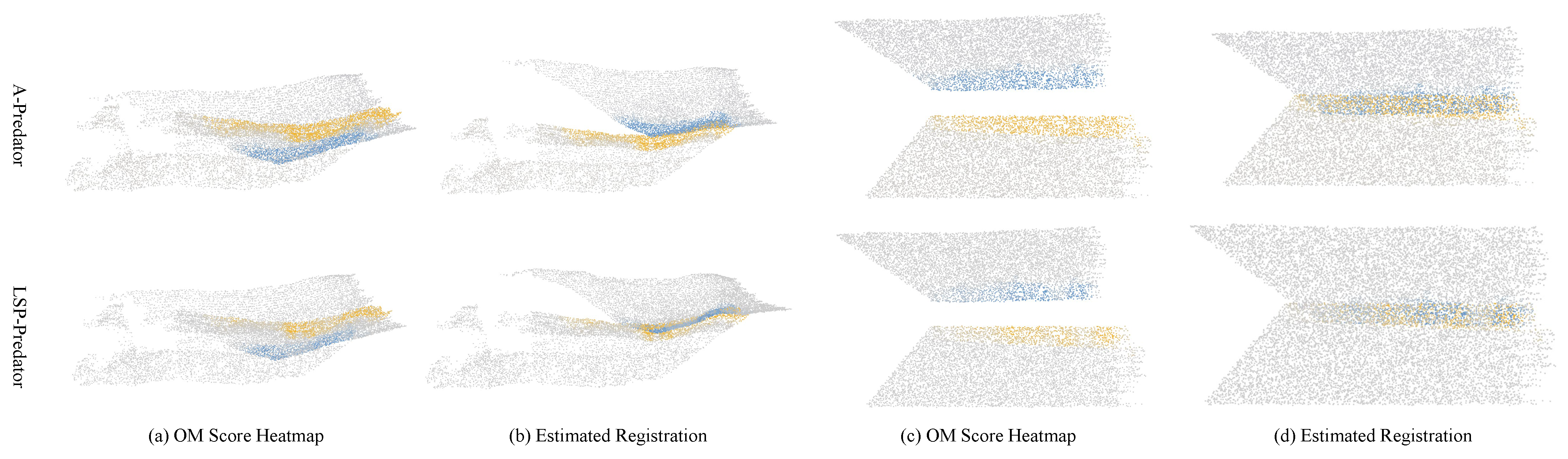
LSP-Predator’s feature-level anisotropic weighting explains its advantage over PAI-Predator across most metrics. Under high-overlap conditions, LSP-Predator approaches A-Predator’s accuracy, suggesting that feature-based anisotropic weighting can be effective when contextual information is abundant. Figure 6a corroborates this, with both methods showing concentrated high-confidence predictions in a feature-rich 40% overlap case.

However, LSP-Predator degrades sharply as overlap decreases (recall drops to 39.70% at 10% overlap). As Figure 6c illustrates, in the 12.5% overlap case, LSP-Predator’s points with high overlap–matching (OM) scores are significantly more dispersed than those of A-Predator, which maintains a compact response around the overlapping region. We attribute this to the absence of spatial receptive field deformation: without aligning the kernel geometry with local principal directions, the model struggles to extract meaningful structural features from sparse, noisy neighborhoods, leading to ambiguous overlap detection under low-overlap conditions.

The design-choice ablation in Table 5 further supports this interpretation. Under the same optimization budget and with the official fitting and repulsive regularization retained, deformable KPConv recovers part of the improvement but yields roughly twice the errors of A3-Predator at 10% overlap. This result suggests that explicit geometric alignment is an important contributor to the observed gain under the evaluated MBES setting. The small and mixed changes from A3-Predator to A4-Predator indicate diminishing returns from replacing deeper blocks in this ablation.

In contrast, A-KPConv’s PCA-based geometric alignment of kernel shape and orientation improves robustness relative to the evaluated alternatives under low-overlap MBES conditions, while remaining sensitive to extremely sparse or nearly degenerate neighborhoods.

5.4. Generalization Capability

The cross-dataset results in Table 6 reveal a consistent pattern: after a single global rescaling of LQL-MBES to the Dotson-east spatial scale, A-Predator achieves higher recall than Predator, LSP-Predator, and GeoTransformer at all evaluated overlap ratios without fine-tuning. The performance gap is most pronounced under low-overlap conditions. At 12.5% overlap, A-Predator achieves 37.25% recall compared with 23.68% for Predator and 8.90% for GeoTransformer. A-Predator also has the lowest reported translation and rotation errors at each level; because these errors are averaged over the successful registrations of each method, they should be interpreted together with recall rather than as unconditional errors over an identical pair subset.

One possible explanation for this transfer result concerns the features learned by each model. Standard KPConv, with its rigid isotropic kernels, may rely more strongly on dataset-specific macroscopic patterns—such as the characteristic swath width and point density of the Dotson-east deep-water acquisition—as discriminative cues. When these patterns differ in a new environment (e.g., the shallow-water, narrow-swath LQL-MBES setting), such features may become less reliable. In contrast, A-KPConv, through its PCA-driven adaptation to local geometry, is encouraged to rely on intrinsic structural properties of the point cloud—principal directions, local curvature, and neighborhood anisotropy—rather than dataset-level statistics. These geometric representations are more likely to remain valid across different acquisition conditions, water depths, and sonar configurations, thereby supporting more effective transfer to unseen underwater environments.

5.5. Failure Cases and Limitations

To understand when and why A-Predator underperforms, we conducted a separate pair-level diagnostic run on the fixed Dotson-east test pairs, using the same trained checkpoints and evaluation protocol as the main experiment but an independent RANSAC random seed. The resulting statistics are therefore used to characterize failure patterns rather than to reproduce the aggregate values in Table 1 exactly. Approximately three quarters of the failed pairs (RRE $>5^{\circ }$ or RTE $>10$ m) have an effective overlap below 0.20 (median 0.13, versus 0.46 for successful pairs), and about 70% exhibit catastrophic divergence (RRE $>{30}^{\circ }$ or RTE $>30$ m) rather than near-threshold deviations. Many of the most difficult pairs also fail under the Predator baseline, which is consistent with shared data-level challenges but does not by itself isolate the cause of failure. Failures also cluster in specific mission segments: at matched effective overlap (0.10–0.20), the failure rate in the latter portion of the survey is about 5.7 times that of the earlier portion. This pattern coincides with a concentration of 180° turnaround maneuvers—where the swath geometry rotates rapidly and the inter-submap overlap collapses—and with INS/positioning drift that can distort submaps stacked from 100 consecutive pings.

Terrain and data quality impose further limitations. Repetitive, self-similar patterns (e.g., sand-wave fields) produce similar descriptors at many locations and can steer RANSAC toward a false consensus, while on flat or feature-poor seafloor the descriptors lose distinctiveness and the captured anisotropy is dominated by the acquisition pattern (dense across-track ping rows) rather than by terrain structure. Extremely sparse regions near swath edges leave too few neighbors for stable per-neighborhood PCA; moderate noise and isolated outliers are largely tolerated thanks to the learned scoring and noise-jitter augmentation, but locally dense outlier clusters can still corrupt the non-learned covariance estimation. Under extremely low overlap, random cropping during data preparation may also remove the overlapping region entirely, and in weak-structure neighborhoods the estimated principal directions may jitter (cf. Section 3.3). Overall, registration performance is jointly affected by seafloor geomorphology, water depth (which controls the acoustic footprint and point spacing), sonar configuration, point density, and motion distortion; potential remedies include outlier-aware covariance estimation, adaptive PCA neighborhood radius selection, and low-cost motion priors, which we leave for future work.

6. Conclusions

In this paper, we address the challenge that existing deep learning-based registration methods do not fully exploit the strong anisotropy and strip-like structures of MBES point clouds. To this end, we propose A-KPConv, a novel anisotropic kernel convolution operator that aligns the convolution kernel with local principal directions via a PCA-based affine transformation. By integrating A-KPConv into the shallow encoder layers of Predator, we further develop A-Predator, a registration model tailored for MBES point clouds.

Extensive experiments on the public Dotson-east dataset and the self-collected LQL-MBES dataset demonstrate that A-Predator achieves the highest registration recall among the evaluated methods and consistently low error metrics across the evaluated overlap levels. On Dotson-east, recall improves from 31.63% to 59.55% at the extremely challenging 10% overlap setting, and similar gains are observed on the LQL-MBES dataset. Ablation studies support the effectiveness of PCA-driven kernel deformation relative to the evaluated anisotropic operators and the advantage of explicit geometric alignment under the evaluated settings. Cross-dataset evaluation further shows that A-Predator, trained solely on Dotson-east, transfers more effectively than the evaluated baselines to the globally rescaled LQL-MBES target without fine-tuning; broader generalization across acquisition conditions remains to be evaluated.

Despite these improvements, our approach has limitations. The reliance on PCA-based direction estimation introduces computational overhead and sensitivity to the neighborhood radius and extreme sparsity (Section 4.5, Section 4.6 and Section 5.5). Future work could explore learning-based alternatives for direction estimation, multi-sensor fusion with inertial and acoustic Doppler velocity measurements from underwater vehicles for joint optimization, and extension of the anisotropic convolution paradigm to other underwater perception tasks such as semantic segmentation and object detection.

References

1. Zhang, J.; Singh, S. Visual-lidar odometry and mapping: Low-drift, robust, and fast. In Proceedings of the 2015 IEEE International Conference on Robotics and Automation (ICRA); IEEE: Piscataway, NJ, USA, 2015; pp. 2174–2181. [Google Scholar]
2. Choi, S.; Zhou, Q.Y.; Koltun, V. Robust reconstruction of indoor scenes. In Proceedings of the IEEE Conference on Computer Vision and Pattern Recognition; IEEE: Piscataway, NJ, USA, 2015; pp. 5556–5565. [Google Scholar]
3. Cadena, C.; Carlone, L.; Carrillo, H.; Latif, Y.; Scaramuzza, D.; Neira, J.; Reid, I.; Leonard, J.J. Past, present, and future of simultaneous localization and mapping: Toward the robust-perception age. IEEE Trans. Robot. 2017, 32, 1309–1332. [Google Scholar] [CrossRef] [Scilit]
4. Joshi, B.; Xanthidis, M.; Roznere, M.; Burgdorfer, N.J.; Mordohai, P.; Li, A.Q.; Rekleitis, I. Underwater exploration and mapping. In Proceedings of the 2022 IEEE/OES Autonomous Underwater Vehicles Symposium (AUV); IEEE: Piscataway, NJ, USA, 2022; pp. 1–7. [Google Scholar]
5. Brown, C.J.; Blondel, P. Developments in the application of multibeam sonar backscatter for seafloor habitat mapping. Appl. Acoust. 2009, 70, 1242–1247. [Google Scholar] [CrossRef] [Scilit]
6. Zhang, F.; Tan, T.; Hou, X.; Zhao, L.; Cao, C.; Wang, Z. Underwater Mapping and Optimization Based on Multibeam Echo Sounders. J. Mar. Sci. Eng. 2024, 12, 1222. [Google Scholar] [CrossRef] [Scilit]
7. Besl, P.J.; McKay, N.D. Method for registration of 3-D shapes. In Proceedings of the Sensor Fusion IV: Control Paradigms and Data Structures; SPIE: Bellingham, WA, USA, 1992; Volume 1611, pp. 586–606. [Google Scholar]
8. Chen, Y.; Medioni, G. Object modelling by registration of multiple range images. Image Vis. Comput. 1992, 10, 145–155. [Google Scholar] [CrossRef] [Scilit]
9. Segal, A.; Haehnel, D.; Thrun, S. Generalized-icp. In Proceedings of the Robotics: Science and Systems, Seattle, WA, USA, 28 June–1 July 2009; Volume 2, p. 435. [Google Scholar]
10. Wang, Y.; Solomon, J.M. Deep closest point: Learning representations for point cloud registration. In Proceedings of the IEEE/CVF International Conference on Computer Vision; IEEE: Piscataway, NJ, USA, 2019; pp. 3523–3532. [Google Scholar]
11. Choy, C.; Park, J.; Koltun, V. Fully convolutional geometric features. In Proceedings of the IEEE/CVF International Conference on Computer Vision; IEEE: Piscataway, NJ, USA, 2019; pp. 8958–8966. [Google Scholar]
12. Choy, C.; Dong, W.; Koltun, V. Deep global registration. In Proceedings of the IEEE/CVF Conference on Computer Vision and Pattern Recognition; IEEE: Piscataway, NJ, USA, 2020; pp. 2514–2523. [Google Scholar]
13. Thomas, H.; Qi, C.R.; Deschaud, J.E.; Marcotegui, B.; Goulette, F.; Guibas, L.J. Kpconv: Flexible and deformable convolution for point clouds. In Proceedings of the IEEE/CVF International Conference on Computer Vision; IEEE: Piscataway, NJ, USA, 2019; pp. 6411–6420. [Google Scholar]
14. Wang, Y.; Sun, Y.; Liu, Z.; Sarma, S.E.; Bronstein, M.M.; Solomon, J.M. Dynamic graph cnn for learning on point clouds. ACM Trans. Graph. (TOG) 2019, 38, 1–12. [Google Scholar] [CrossRef] [Scilit]
15. Huang, S.; Gojcic, Z.; Usvyatsov, M.; Wieser, A.; Schindler, K. Predator: Registration of 3d point clouds with low overlap. In Proceedings of the IEEE/CVF Conference on Computer Vision and Pattern Recognition; IEEE: Piscataway, NJ, USA, 2021; pp. 4267–4276. [Google Scholar]
16. Ling, L.; Zhang, J.; Bore, N.; Folkesson, J.; Wåhlin, A. Benchmarking classical and learning-based multibeam point cloud registration. In Proceedings of the 2024 IEEE International Conference on Robotics and Automation (ICRA); IEEE: Piscataway, NJ, USA, 2024; pp. 6118–6125. [Google Scholar]
17. Qi, C.R.; Su, H.; Mo, K.; Guibas, L.J. Pointnet: Deep learning on point sets for 3d classification and segmentation. In Proceedings of the IEEE Conference on Computer Vision and Pattern Recognition; IEEE: Piscataway, NJ, USA, 2017; pp. 652–660. [Google Scholar]
18. Qi, C.R.; Yi, L.; Su, H.; Guibas, L.J. Pointnet++: Deep hierarchical feature learning on point sets in a metric space. Adv. Neural Inf. Process. Syst. 2017, 30, 5105–5114. [Google Scholar]
19. Qian, G.; Li, Y.; Peng, H.; Mai, J.; Hammoud, H.; Elhoseiny, M.; Ghanem, B. Pointnext: Revisiting pointnet++ with improved training and scaling strategies. Adv. Neural Inf. Process. Syst. 2022, 35, 23192–23204. [Google Scholar] [CrossRef] [Scilit]
20. Simonovsky, M.; Komodakis, N. Dynamic edge-conditioned filters in convolutional neural networks on graphs. In Proceedings of the IEEE Conference on Computer Vision and Pattern Recognition; IEEE: Piscataway, NJ, USA, 2017; pp. 3693–3702. [Google Scholar]
21. Zhou, H.; Feng, Y.; Fang, M.; Wei, M.; Qin, J.; Lu, T. Adaptive graph convolution for point cloud analysis. In Proceedings of the IEEE/CVF International Conference on Computer Vision; IEEE: Piscataway, NJ, USA, 2021; pp. 4965–4974. [Google Scholar]
22. Xu, Y.; Fan, T.; Xu, M.; Zeng, L.; Qiao, Y. Spidercnn: Deep learning on point sets with parameterized convolutional filters. In Proceedings of the European Conference on Computer Vision (ECCV); IEEE: Piscataway, NJ, USA, 2018; pp. 87–102. [Google Scholar]
23. Li, Y.; Bu, R.; Sun, M.; Wu, W.; Di, X.; Chen, B. Pointcnn: Convolution on x-transformed points. Adv. Neural Inf. Process. Syst. 2018, 31, 828–838. [Google Scholar]
24. Xu, M.; Ding, R.; Zhao, H.; Qi, X. Paconv: Position adaptive convolution with dynamic kernel assembling on point clouds. In Proceedings of the IEEE/CVF Conference on Computer Vision and Pattern Recognition; IEEE: Piscataway, NJ, USA, 2021; pp. 3173–3182. [Google Scholar]
25. Wu, W.; Qi, Z.; Fuxin, L. Pointconv: Deep convolutional networks on 3d point clouds. In Proceedings of the IEEE/CVF Conference on Computer Vision and Pattern Recognition; IEEE: Piscataway, NJ, USA, 2019; pp. 9621–9630. [Google Scholar]
26. Vaswani, A.; Shazeer, N.; Parmar, N.; Uszkoreit, J.; Jones, L.; Gomez, A.N.; Kaiser, Ł.; Polosukhin, I. Attention is all you need. Adv. Neural Inf. Process. Syst. 2017, 30, 6000–6010. [Google Scholar]
27. Guo, M.H.; Cai, J.X.; Liu, Z.N.; Mu, T.J.; Martin, R.R.; Hu, S.M. Pct: Point cloud transformer. Comput. Vis. Media 2021, 7, 187–199. [Google Scholar] [CrossRef] [Scilit]
28. Zhao, H.; Jiang, L.; Jia, J.; Torr, P.H.; Koltun, V. Point transformer. In Proceedings of the IEEE/CVF International Conference on Computer Vision; IEEE: Piscataway, NJ, USA, 2021; pp. 16259–16268. [Google Scholar]
29. Yu, X.; Tang, L.; Rao, Y.; Huang, T.; Zhou, J.; Lu, J. Point-bert: Pre-training 3d point cloud transformers with masked point modeling. In Proceedings of the IEEE/CVF Conference on Computer Vision and Pattern Recognition; IEEE: Piscataway, NJ, USA, 2022; pp. 19313–19322. [Google Scholar]
30. Pang, Y.; Tay, E.H.F.; Yuan, L.; Chen, Z. Masked autoencoders for 3d point cloud self-supervised learning. World Sci. Annu. Rev. Artif. Intell. 2023, 1, 2440001. [Google Scholar] [CrossRef] [Scilit]
31. Yu, H.; Li, F.; Saleh, M.; Busam, B.; Ilic, S. Cofinet: Reliable coarse-to-fine correspondences for robust pointcloud registration. Adv. Neural Inf. Process. Syst. 2021, 34, 23872–23884. [Google Scholar]
32. Qin, Z.; Yu, H.; Wang, C.; Guo, Y.; Peng, Y.; Ilic, S.; Hu, D.; Xu, K. Geotransformer: Fast and robust point cloud registration with geometric transformer. IEEE Trans. Pattern Anal. Mach. Intell. 2023, 45, 9806–9821. [Google Scholar] [CrossRef] [Scilit] [PubMed]
33. Ao, S.; Hu, Q.; Wang, H.; Xu, K.; Guo, Y. Buffer: Balancing accuracy, efficiency, and generalizability in point cloud registration. In Proceedings of the IEEE/CVF Conference on Computer Vision and Pattern Recognition; IEEE: Piscataway, NJ, USA, 2023; pp. 1255–1264. [Google Scholar]
34. Fu, K.; Yuan, M.; Wang, C.; Pang, W.; Chi, J.; Wang, M.; Gao, L. Dual Focus-Attention Transformer for Robust Point Cloud Registration. In Proceedings of the Computer Vision and Pattern Recognition Conference; IEEE: Piscataway, NJ, USA, 2025; pp. 11769–11778. [Google Scholar]
35. Gao, Z.; Zhai, G.; Yan, J.; Yang, X. Permutation matters: Anisotropic convolutional layer for learning on point clouds. arXiv 2020, arXiv:2005.13135. [Google Scholar]
36. Wiersma, R.; Nasikun, A.; Eisemann, E.; Hildebrandt, K. Deltaconv: Anisotropic operators for geometric deep learning on point clouds. ACM Trans. Graph. (TOG) 2022, 41, 1–10. [Google Scholar]
37. Zhang, H.; Wang, K.; Zhong, C.; Yun, K.; Wang, Z.; Yang, Y.; Tao, X. LSPConv: Local spatial projection convolution for point cloud analysis. PeerJ Comput. Sci. 2024, 10, e1738. [Google Scholar] [CrossRef] [Scilit] [PubMed]
38. Zhao, L.; Cheng, L.; Tan, T.; Cao, C.; Zhang, F. Fast and Deterministic Underwater Point Cloud Registration for Multibeam Echo Sounder Data. J. Mar. Sci. Eng. 2024, 13, 26. [Google Scholar] [CrossRef] [Scilit]
39. Torroba, I.; Sprague, C.I.; Bore, N.; Folkesson, J. PointNetKL: Deep inference for GICP covariance estimation in bathymetric SLAM. IEEE Robot. Autom. Lett. 2020, 5, 4078–4085. [Google Scholar] [CrossRef] [Scilit]
40. Tan, J.; Torroba, I.; Xie, Y.; Folkesson, J. Data-driven loop closure detection in bathymetric point clouds for underwater slam. arXiv 2022, arXiv:2209.08578. [Google Scholar]
41. Sun, Y.; Cheng, C.; Zhang, Y.; Zhang, C.; Zheng, L.; Wang, Z.; Wei, Y. Circle loss: A unified perspective of pair similarity optimization. In Proceedings of the IEEE/CVF Conference on Computer Vision and Pattern Recognition; IEEE: Piscataway, NJ, USA, 2020; pp. 6398–6407. [Google Scholar]
42. Rusu, R.B.; Blodow, N.; Beetz, M. Fast point feature histograms (FPFH) for 3D registration. In Proceedings of the 2009 IEEE International Conference on Robotics and Automation; IEEE: Piscataway, NJ, USA, 2009; pp. 3212–3217. [Google Scholar]
43. Fischler, M.A.; Bolles, R.C. Random sample consensus: A paradigm for model fitting with applications to image analysis and automated cartography. Commun. ACM 1981, 24, 381–395. [Google Scholar]
Figure 1. Comparison of point cloud registration performance by different methods on low-overlap submaps. The source point cloud is shown in blue, and the target point cloud is in yellow. The figure illustrates the visualization results of multibeam echosounder (MBES) point cloud registration. Specifically, (a,b) represent test cases from the Dotson-east dataset with a 10% overlap, while (c) represents a test case from the LQL-MBES dataset with a 12.5% overlap.
Remotesensing 18 03035 g001
Figure 2. Schematic diagrams of the network structures. (a) ResNet Bottleneck KPConv structure. (b) Graph Neural Network structure.
Remotesensing 18 03035 g002
Figure 3. Schematic diagram of the A-KPConv module operation. The number of neighboring points within the kernel range, denoted | N p x | in Equation (5), varies from one convolution center to another. For each center point, the features of its neighboring points are weighted by the influences of all kernel points and aggregated using the corresponding convolution weight matrices, where the correlation coefficient h (Equation (9)) depends on the relative position of the neighboring point with respect to the kernel point.
Remotesensing 18 03035 g003
Figure 4. A-Predator network architecture. The encoder ((left), blue panel) is a stack of residual convolution blocks; only the first three blocks from the input side differ from the original Predator encoder and are highlighted in warm colors: the first is a Simple A-KPConv block (orange), and the second and third are ResNet Bottleneck A-KPConv (RBAKPC) blocks (yellow and lavender, respectively), the third operating with stride. All subsequent blocks are the original RBKPC blocks (white; strided downsampling blocks shown in blue), and “(x2)” denotes two consecutive identical blocks. The Overlap Attention module (top) and the decoder (middle) are identical to those of the original Predator. The (bottom) panel expands the internal structures of the RBAKPC block and the GNN module. F s and F t denote the extracted features of the source and target point clouds, and o s , o t and m s , m t denote the corresponding overlap and matching scores.
Remotesensing 18 03035 g004
Figure 5. (a) depicts the field experimental site. (b) shows the experimental platform mounted on the survey vessel, with the key onboard devices indicated by colored boxes: the global navigation satellite system (GNSS) antennas (blue), the inertial navigation system (INS, red), and the HDY-BD400D multibeam echosounder (orange, pole-mounted over the side of the vessel and also shown in the close-up inset; its main specifications are listed in Table 2). The solid arrows connect each colored box with the corresponding device label, while the dashed orange arrows indicate the correspondence between the pole-mounted multibeam echosounder and its close-up inset.
Remotesensing 18 03035 g005
Figure 6. Comparison of OM score heatmaps and the corresponding registration results for A-Predator (top row) and LSP-Predator (bottom row) under two scenarios. (a) OM score heatmap and (b) estimated registration for the Dotson-east case with 40% overlap (feature-rich terrain); (c) OM score heatmap and (d) estimated registration for the LQL-MBES case with 12.5% overlap (fewer features). OM represents the product of the overlap score and the matching score. In (a,c), points with high OM scores are shown in blue (source point cloud) and yellow (target point cloud), while points with low OM scores are shown in gray; in (b,d), the source point cloud is shown in blue and the target point cloud in yellow.
Remotesensing 18 03035 g006