High-Spatiotemporal-Resolution Remote Sensing Retrieval of Evapotranspiration with Sentinel-2 Data by Sharpening MODIS Land Surface Temperature

Highlights

What are the main findings?

• The study improves the spatial details and physical rationality of MODIS LST by incorporating auxiliary variables into the DMS sharpening method markedly, and obtains the downscaled 10 m LST and Sentinel-2-derived 10 m ET.
• The study supplements Sentinel-2-derived 10 m ET into high-spatial-resolution ET of UWET, which fills temporal data gaps and improves fused ET accuracy.

What are the implications of the main findings?

• The improved LST sharpening scheme enables reliable high-resolution ET retrieval from Sentinel-2, overcoming Sentinel-2’s inherent problem of the lack of a thermal infrared sensor for regional farmland evapotranspiration monitoring.
• The established fusion workflow may be applied to similar agricultural regions to produce continuous daily high-spatial-resolution ET data, supporting refined irrigation scheduling and local water resource management.

Abstract

High-spatiotemporal-resolution evapotranspiration (ET) is critical for precision irrigation management and water resource regulation. Regarding the existing spatiotemporal fusion methods suffering from sparse high-resolution observations and coarse land surface temperature (LST), this study took winter wheat in Luancheng District, Hebei Province, as the research object, and proposed a remote sensing ET retrieval method based on the LST sharpening model. The Data Mining Sharpener (DMS) algorithm combined with Sentinel-2 multispectral data was used to downscale MODIS LST from 1000 m to 10 m, with auxiliary variables (DEM, albedo, NDVI, land cover) integrated into the Cubist regression tree to improve the physical rationality and spatial details of MODIS LST. The 10 m resolution ET was estimated from 10 m sharpened LST and Sentinel-2 multispectral data using the surface energy balance model, and the unmixing–weight ET image fusion model (UWET) was adopted to fuse the 10 m resolution ET with MODIS low-resolution ET to generate a daily 10 m ET dataset covering the entire winter wheat growing season. Validation with eddy covariance flux measurements showed that the correlation coefficient R = 0.921, RMSE = 0.779 mm/day during 2019–2020, and R = 0.900, RMSE = 0.831 mm/day during 2020–2021. The results demonstrate that auxiliary variables significantly enhance the spatial reality of LST, LST sharpening effectively improves the spatial heterogeneity of ET, and Sentinel-2 data compensates for the temporal deficiency of Landsat, thereby greatly promoting the accuracy of spatiotemporal fusion. This method can provide reliable high-spatiotemporal-resolution data support for refined farmland irrigation management and water resources regulation.

1. Introduction

Evapotranspiration (ET) with high spatiotemporal resolution is of great significance for refined irrigation management, water resources regulation, and crop growth monitoring [1,2,3]. At the regional scale, remote sensing data for ET retrieval are categorized into high-temporal-resolution and high-spatial-resolution images [4,5]. ET with high spatial resolution is commonly applied to identify spatial characteristics and distribution patterns of ET, such as ET from the Landsat satellite series. In contrast, ET with high temporal resolution is primarily used to monitor the dynamic variations in ET in long time series, such as the MOD16 (1 km) and GLASS products (0.05°) [6]. However, the aforementioned two types of ET products cannot provide data with high temporal and high spatial resolution at the same time, and do not simultaneously meet the requirements of systematic strategies in water resource and irrigation management [7,8].

Spatiotemporal fusion methods have been introduced to generate ET with both high spatial and high temporal resolution [9]. Gao et al. proposed the Spatial and Temporal Adaptive Reflectance Fusion Model (STARFM), which established a weighting relationship between different resolution reflectance data and computed a high-resolution image for the target date within a moving window [10]. Zhu et al. introduced a transformation coefficient to improve the weighting mechanism of STARFM and proposed the ESTARFM method [11]. Zhang et al. introduced Sentinel-2 land cover data, replaced the resampling step with spectral unmixing, and proposed the UWET method, which estimated ET with 10 m spatiotemporal resolution [12]. However, in the above fusion methods, both the quality and the quantity of high-spatial-resolution data may significantly affect the final fusion results [13]. Landsat data provide multispectral data with 30 m resolution and thermal infrared data with 100 m resolution, and are frequently used as a source of high-spatial-resolution ET data in spatiotemporal fusion methods [14]. Nevertheless, its 16-day re-entry period restricts broader applications, and the data availability is further constrained by cloud contamination. Errors of ET estimation increase rapidly as the re-entry period increases [15]. Therefore, data with both high spatial and high temporal resolution is essential for accurate daily ET estimation.

Currently, many satellites equipped with multispectral sensors, such as Sentinel-2 and the Gaofen (GF) series, are capable of acquiring data with both high spatial and temporal resolution. Nevertheless, ET retrieval is highly dependent on land surface temperature (LST), particularly within energy balance models, where LST plays a critical role in determining the accuracy of potential and actual estimates of evapotranspiration [16]. Due to the inherent limitations of thermal infrared sensors, the spatial resolution of satellite-derived LST products remains relatively coarse [17]. The shortage of high-quality LST data has therefore posed a major constraint on the generation of high-spatiotemporal-resolution ET datasets. Sentinel-2 data provide multispectral data with 10 m spatial resolution and a 5-day re-entry period, and have been widely applied in land surface monitoring. Sentinel-2 data can capture short-term dynamics of ET while simultaneously enhancing spatial resolution and providing richer spatial detail for applications at local scales. However, the absence of a thermal infrared sensor prevents Sentinel-2 multispectral data from being directly utilized for ET estimation. LST with high spatiotemporal resolution is urgently needed for Sentinel-2.

A quite reliable LST product is the global LST product of the MOD11 series. The accuracy of ground verification can reach 1 K [18], but with a resolution of 1000 m. Downscaling is considered one of the effective methods to obtain LST with higher spatial resolution [19]. Existing downscaling methods can be broadly classified into two categories: methods based on statistical regression and methods based on spatiotemporal image fusion. Methods based on statistical regression assume that the relationship between low-resolution LST and auxiliary variables remains stable within a given region, and then apply this relationship to higher-resolution data. Kustas et al. proposed the TsHARP method, which established four functional forms between LST and the normalized difference vegetation index (NDVI), and constructed polynomial regression relationships between them [20,21]. Gao et al. introduced the Data Mining Sharpener (DMS) method, which uses fundamental reflectance data as a variable and employs regression trees to model the relationship between LST and reflectance [22]. Guzinski et al. applied the DMS method to sharpen 1 km thermal infrared data from Sentinel-3, combining it with Sentinel-2 shortwave multispectral data to estimate high-spatial-resolution ET, and the method yielded promising results with the relative RMSE of instantaneous latent heat flux around 30% [23,24,25]. Methods based on spatiotemporal image fusion, on the other hand, rely on high-resolution imagery as the basis to be fused with low-resolution data. A typical example is the STARFM, which has been widely used not only for reflectance fusion but also for LST fusion. However, considering that Sentinel-2 lacks a thermal infrared sensor, yet provides high-resolution multispectral bands suitable for retrieving land surface parameters, statistical regression-based approaches are generally more appropriate for Sentinel-2.

The problem with spatiotemporal fusion models of evapotranspiration is scarce high-spatial-resolution ET data. To address this problem, this study combined Sentinel-2 multispectral data with the Data Mining Sharpener (DMS) method to sharpen MODIS LST products, thereby generating LST data at a spatial resolution of 10 m for the study area. Furthermore, Sentinel-2 data and sharpened LST data are input into the SEBAL model as surface parameters. Evapotranspiration with a resolution of 10 m from Sentinel-2 data was calculated as the high-spatial-resolution data for the spatiotemporal fusion models of ET. The UWET was selected for spatiotemporal fusion, and we unmixed MODIS-derived ET using land cover maps to 10 m resolution and incorporated the results into subsequent weight calculations, making it particularly suitable for high-resolution ET fusion based on Sentinel-2 data. Finally, a high-spatiotemporal-resolution ET dataset for winter wheat in Luancheng District, Hebei Province, was produced. The results were evaluated at both temporal and spatial scales, and the implications of LST sharpening were also discussed.

2. Study Area and Data

2.1. Study Area

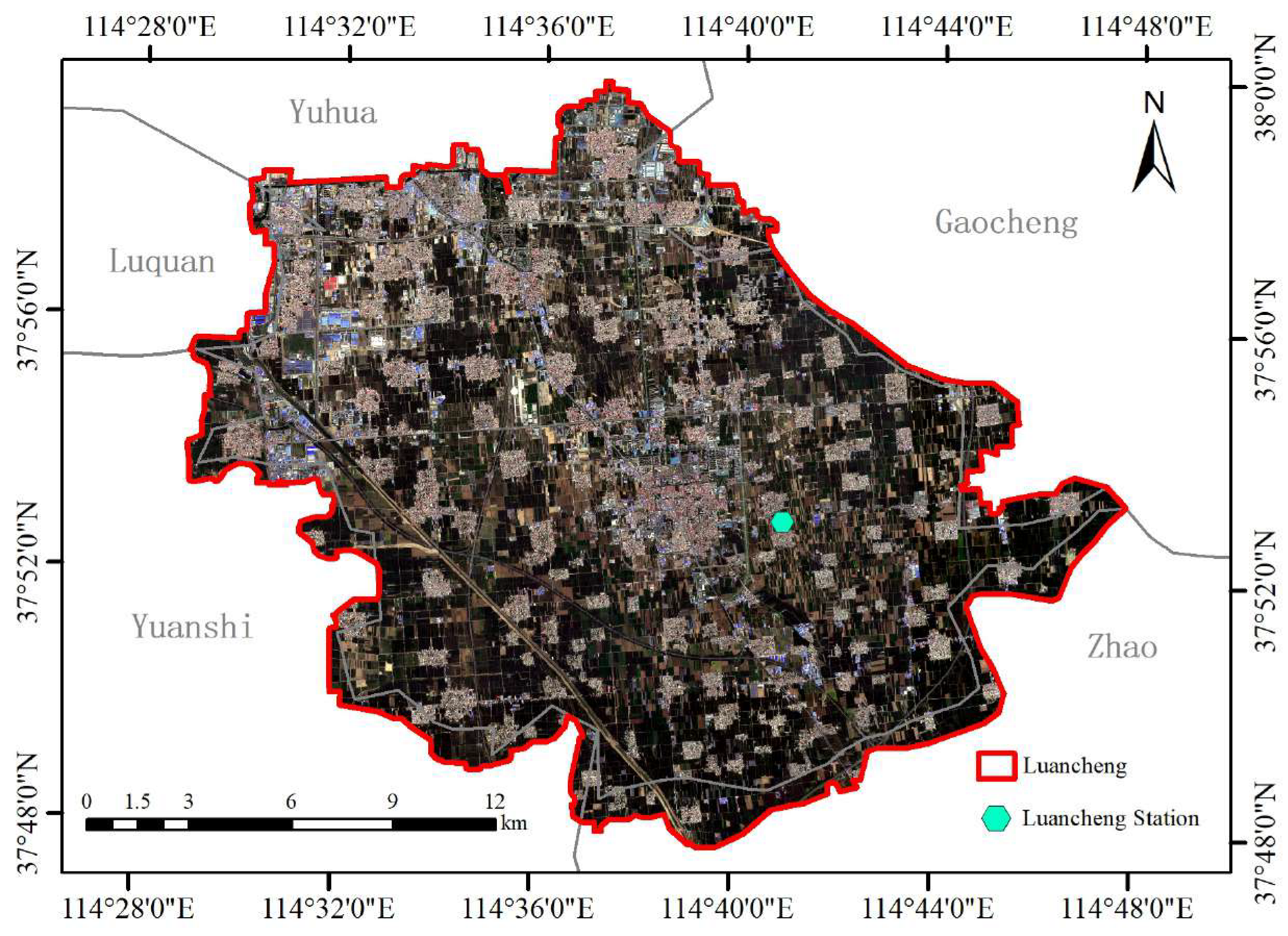
The study area is Luancheng District, Shijiazhuang City, Hebei Province (37°59′20″–37°47′34″N, 114°28′36″–114°47′35″E), as shown in Figure 1. The region is characterized by a temperate continental monsoon climate, falling within the warm temperate semi-humid zone, and its dominant agricultural system is a winter wheat–summer maize rotation. Luancheng District covers an area of approximately 345 square kilometers, with terrain gently sloping from the northwest to the southeast and elevations ranging between 40 and 60 m. The primary cropping system is a two-crop-a-year rotation of winter wheat and summer corn, and the planting structure is highly monotonous; the winter wheat planting area is about 164 square kilometers. Within the study area, the Luancheng flux observation station (37°53′N, 114°41′E) has been established, enabling real-time monitoring of ecosystem fluxes.

2.2. Data Description

In this study, ET at a spatial resolution of 10 m was calculated using Landsat-8 data, Sentinel-2 data, and the sharpened LST. Additionally, MODIS satellite products—including the daily MOD09GA surface reflectance (500 m), MCD43A3 surface albedo (500 m), and MOD11A1 land surface temperature (1000 m)—were employed to retrieve daily ET at a spatial resolution of 500 m for the study area. Although the MOD16 series also provides standard ET products, these are generated using a unified algorithm primarily designed for large-scale spatiotemporal applications and for maintaining temporal continuity. Given the relatively small extent of the study area, daily ET was instead estimated from the more fundamental MODIS data products, allowing for the incorporation of local parameters (e.g., meteorological and elevation data) to improve model accuracy. Flux tower observations were used to validate the accuracy of the predicted ET results.

2.2.1. Satellite Data

Sentinel-2 is a series of Earth observation satellites under the Copernicus Program led by the European Space Agency (ESA), with a 5-day re-entry period and 10 m resolution, and equipped with the Multi-Spectral Instrument (MSI). In this study, Sentinel-2 imagery was accessed and preprocessed through the Google Earth Engine platform (https://earthengine.google.com/), and was employed both as an input variable for temperature sharpening and for deriving high-resolution evapotranspiration on reference dates. Only the images with cloud coverage less than 10% were selected.

MODIS data used in this study were downloaded from NASA’s Earth Observing System Data and Information System (https://www.earthdata.nasa.gov//) and preprocessed using the ENVI-MCTK 2.1.13 toolbox for format conversion and resampling. Specifically, three daily MODIS products were selected: MOD09GA surface reflectance, MCD43A3 albedo, and MOD11A1 land surface temperature (LST). All three products were reprojected to the WGS 1984 UTM Zone 50 N coordinate system and resampled to 500 m using cubic convolution. Quality control was performed based on the QC (quality control) band, retaining only cloud-free, clear, high-quality pixels for calculation.

Landsat-8/9 are equipped with the Operational Land Imager (OLI)/OLI-2 multispectral sensors and the thermal infrared sensor (TIRS)/TIRS-2 thermal infrared sensors, which provide a multispectral spatial resolution of 30 m and a thermal infrared spatial resolution of 100 m. Data were obtained from the USGS website (https://www.usgs.gov/) and preprocessed using ENVI 5.6 software. In this study, Landsat data were used for deriving high-resolution evapotranspiration on base dates and as reference datasets to validate the spatial distribution of Sentinel-2-based ET and LST retrievals. Only the images with cloud coverage less than 10% were selected. The DOY used for different data is shown in

Table 1. DOY of data used.

Year	Sentinel-2	Landsat-8/9	MODIS
2019	298, 303, 308, 318, 323, 338, 353	300, 364	274–365
2020	48, 53, 78, 93, 103, 108, 113, 118, 143, 148, 158, 293, 298, 308, 313, 318, 338, 353	47, 63, 79, 95, 111, 143, 351	1–182, 275–366
2021	2, 12, 17, 22, 32, 37, 42, 47, 62, 82, 97, 107, 117, 127, 132, 147, 158, 177	1, 17, 33, 49, 81, 97, 129, 145, 177	1–181

.

2.2.2. Other Data

(1)

Meteorological Data

Meteorological data were from Shijiazhuang meteorological station (ID: 53698, 38.30°N, 114.70°E.) and can be downloaded online (https://data.cma.cn/). The dataset includes key variables such as air temperature, wind speed, atmospheric pressure, and precipitation. Data covering the period from October 2019 to June 2020 were collected and used for the calculation of daily evapotranspiration as well as reference evapotranspiration estimated by the Penman–Monteith equation.

(2)

Validation Data

In situ flux observations were obtained from the Luancheng Station for the period from September 2019 to June 2021 [26]. The dataset includes half-hourly measurements of daily evapotranspiration (ET), latent heat flux, radiation fluxes, and related variables, and was aggregated to obtain daily values for verifying the estimation of evapotranspiration retrieved from satellite data. These observations were collected using an eddy-covariance flux tower and processed following the standardized ChinaFLUX technical protocols, with appropriate adjustments made to account for local meteorological conditions. Data quality was assessed through energy balance closure, where the regression slope between turbulent energy fluxes (the sum of sensible and latent heat fluxes) and available energy (net radiation minus soil heat flux) indicated an energy balance closure of approximately 85%, confirming the reliability of the dataset.

2.3. Land Cover Map

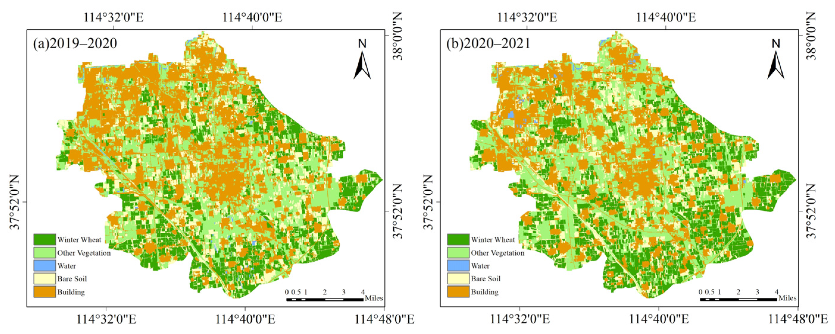
Land cover maps are applied to the LST sharpening model, the SEBAL model, and the spatiotemporal fusion model for evapotranspiration [27]. In this study, land cover maps of the study area were generated based on Sentinel-2 NDVI time series and the multi-resolution segmentation algorithm. Cubic spline interpolation and Savitzky–Golay filtering were adopted to reconstruct NDVI time series for eliminating cloud contamination and random noise, while the multi-resolution segmentation algorithm was used to preserve the integrity of field parcels and reduce salt-and-pepper noise. Based on the results of multiple comparative experiments conducted by eCognition, the optimal segmentation factor was selected. The optimal segmentation scale was determined using the ESP2 tool. By leveraging the mathematical characteristics of the NDVI time series curve and the random forest method, the land cover map was obtained. Land cover maps from 2019 to 2021 are illustrated in Figure 2. Randomly generate sample points on the map, combine multi-spectral features and NDVI curve features to determine the true land type, and use them as the true land surface value to verify the accuracy of the classification results. The results are shown in

Table 2. The confusion matrix of the validation samples.

	Winter Wheat	Other Vegetation	Building	Bare Soil	Water	Total	User Accuracy
Winter Wheat	38	2	0	1	0	41	92.7%
Other Vegetation	1	30	1	0	1	33	90.9%
Building	0	0	20	0	0	20	100%
Bare Soil	1	1	0	13	1	16	81.3%
Water	0	0	1	1	8	10	80.0%
Total	40	33	22	15	10	120
Producer Accuracy	95.0%	90.9%	90.9%	86.7%	80.0%		90.83%

. The overall accuracy is above 90%, and the kappa coefficient is 0.87, which meets the requirements for subsequent applications.

3. Methods

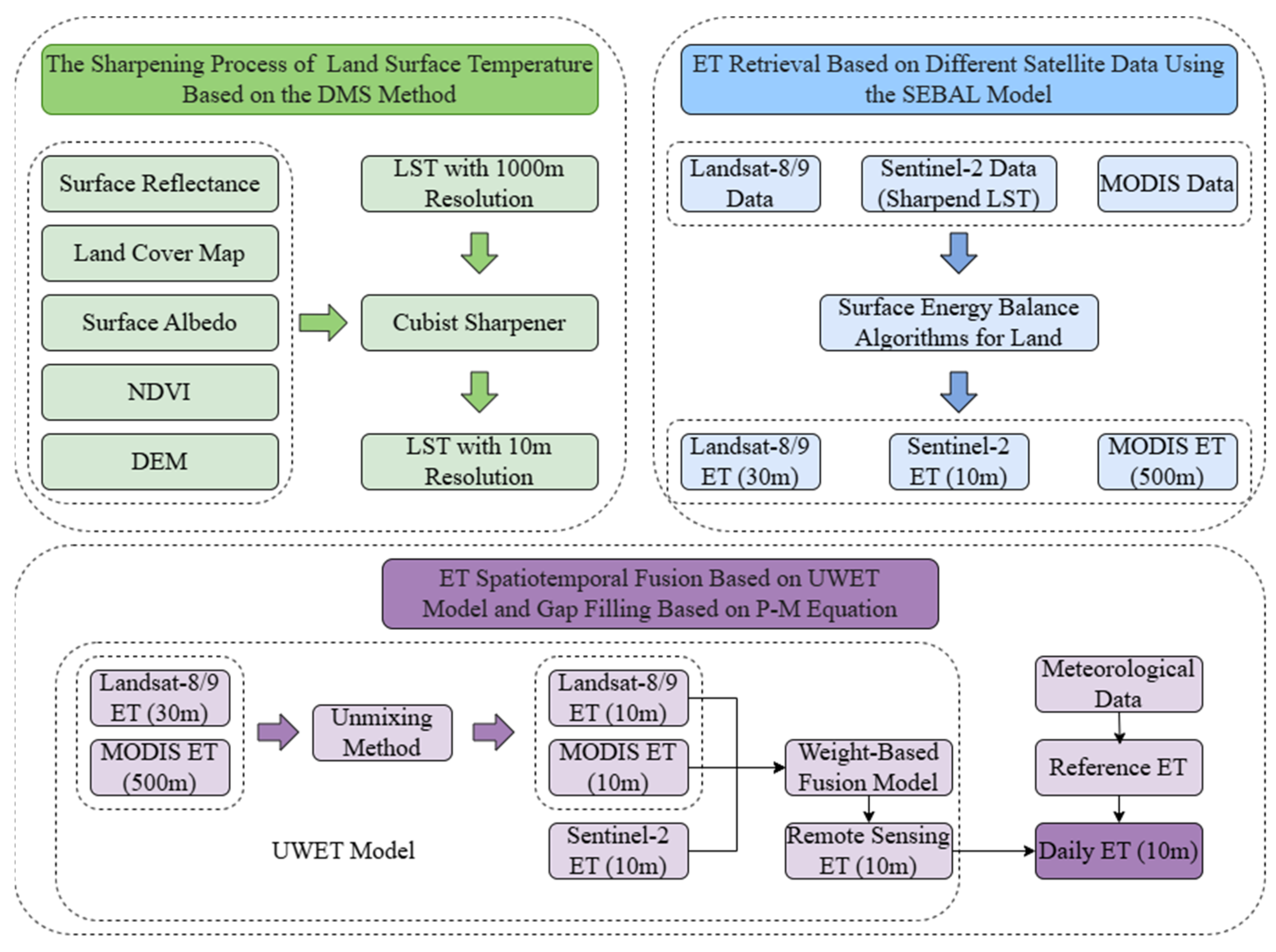
Different bands and land surface parameters of Sentinel-2 data were selected and aggregated to match the coarse resolution of the MOD11A1 LST product. High-quality pixel samples were then extracted to construct a relationship using a regression tree approach, which was subsequently applied to Sentinel-2 high-resolution bands. By incorporating residuals, a 10 m resolution LST dataset was obtained. Based on other land surface variables derived from Sentinel-2, 10 m resolution ET was further estimated. As a supplement to the Landsat ET, these results, together with 500 m resolution ET derived from MODIS products, were integrated into the UWET spatiotemporal fusion model to generate ET with high spatial and temporal resolution. The data used for accuracy verification are the observation data from the Luancheng Station flux tower during the winter wheat growing season from 2019 to 2021. The overall workflow is illustrated in Figure 3.

3.1. LST Sharpening Model

The LST sharpening process was implemented based on the Data Mining Sharpener (DMS) algorithm. Compared with conventional LST sharpening models that rely on empirical relationships, the DMS method avoids the a priori assumption of linear or nonlinear correlations between LST and auxiliary parameters. Instead, it adaptively mines the association rules between LST and input parameters from sample datasets and adopts differentiated variable combinations for diverse surface scenarios. This approach effectively addresses the limitations of traditional thermal sharpening methods over heterogeneous land surfaces and presents outstanding flexibility and diversity in variable selection.

3.1.1. The Selection of Input Variables

Most existing studies take surface reflectance as the sole input of the DMS model and identify the internal correlation between temperature and reflectance through data mining procedures. Nevertheless, single reflectance variables are insufficient and inapplicable for the MODIS LST sharpening in this study. On the one hand, DMS downscales the 1000 m resolution LST of MOD11A1 data to the 10 m resolution corresponding to Sentinel-2 imagery, with a substantially larger downscaling range than that adopted in previous studies. Since the model is trained based on low-resolution samples, the spatially detailed information of reflectance is severely weakened, which makes it difficult to characterize the fine-scale LST heterogeneity under high-resolution conditions. On the other hand, LST is comprehensively regulated by multiple environmental factors, including topographic undulation and land use types, which cannot be fully expressed merely by surface reflectance [17]. The importance of selecting appropriate multi-source auxiliary predictors for statistical downscaling has also been emphasized [28].

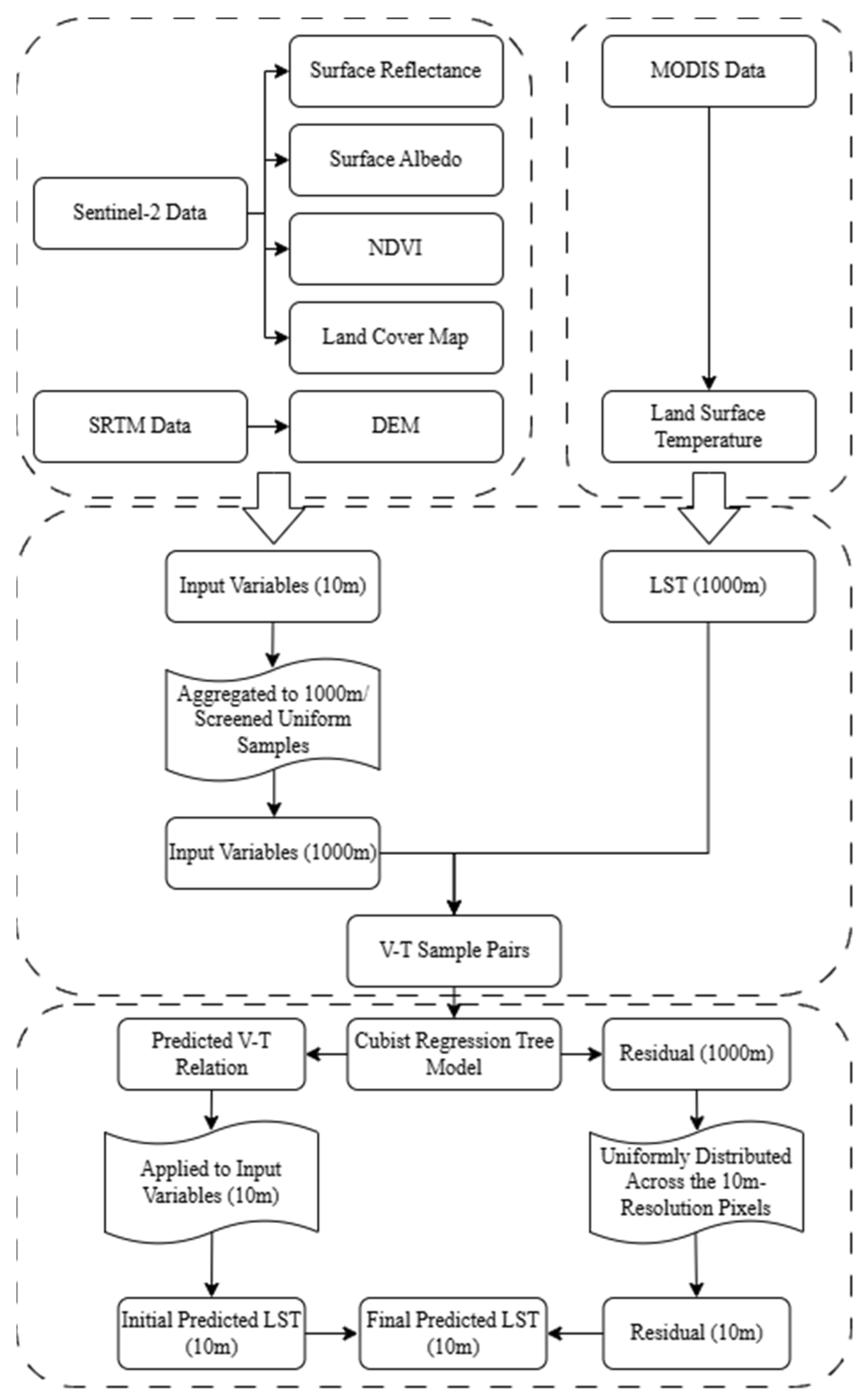
Therefore, in addition to surface reflectance, auxiliary variables involving the digital elevation model (DEM), surface albedo, normalized difference vegetation index (NDVI), and land use type were further incorporated into the DMS model in this study. DEM data can quantitatively reflect the topographic relief of the study area; surface albedo indicates the surface capacity of absorbing solar shortwave radiation; NDVI precisely characterizes the growth status and coverage condition of surface vegetation; land use type enables the model to construct independent temperature simulation rules for different land cover categories, which is conducive to capturing the real spatial distribution of LST under pixel mixed conditions. The detailed information and descriptions of all model input variables are listed in

Table 3. Input Variables.

Number	Input Variables	Source
1	Blue	Sentinel-2 Land Surface Reflectance
2	Green
3	Red
4	RedEdge1
5	RedEdge2
6	RedEdge3
7	NIR
8	RedEdge4
9	SWIR1
10	SWIR2
11	DEM	SRTM 30 m DEM
12	Albedo	Advanced calculation
13	NDVI
14	Land Cover (Wheat)
15	Land Cover (Building)

, and all variables were standardized via normalization processing before model input. Considering that the original categorical variables of land use type showed low sensitivity to model operation, the two dominant land use types in the study area, namely construction land and winter wheat cropland, were converted into binary feature variables for optimized model adaptation. The workflow of the LST sharpening model is shown in Figure 4.

3.1.2. Uniform Training Sample Screening Based on Average Coefficient of Variation

The spatial resolution of the MOD11A1 LST product is 1000 m, while the resolution of input feature variables is 10 m. To establish the statistical relationship between LST and reflectance at the coarse resolution, all input feature variables need to be aggregated to the low resolution prior to relationship modeling, so as to construct complete sample pairs of land surface temperature–input variables. In the downscaling aggregation process from high resolution to low resolution, the aggregation of feature variables follows a linear pattern, whereas the aggregation of land surface temperature is nonlinear. This discrepancy causes the relationship between LST and input features of mixed pixels to vary with spatial resolution. To reduce the errors induced by such variation, it is necessary to ensure that mixed pixels are as homogeneous as possible before aggregation. Accordingly, sample pixels involved in model training require further screening before the relationship model is established. The average coefficient of variation for coarse-resolution mixed pixels is defined as follows:

$$c_v=({\displaystyle \frac{1}{n}}){\displaystyle {\sum }_1^n}({\sigma }_i/{\mu }_i),$$

(1)

where $n$ is the number of spectral bands; $i$ is the i-th spectral band; $\sigma$ is the standard deviation; and $\mu$ is the average value. $c_v$ represents the homogeneity of mixed pixels before aggregation and can eliminate the differences caused by units and orders of magnitude. A smaller $c_v$ value indicates higher homogeneity and better uniformity of mixed pixels. In this study, $c_v$ was used as a criterion to evaluate the homogeneity of mixed pixels. An adaptive $c_v$ threshold was applied to retain 80% of the pixels within the study area for model training, aiming to exclude severely mixed samples while preserving sufficient spatial information and sample diversity [22].

3.1.3. Sharpening Model Training Based on Cubist Regression Tree

In this study, the Cubist algorithm was employed for DMS downscaling training. Cubist is derived from the M5 model tree proposed by Quinlan (1992), with its core concept being the fitting of multivariate linear regression models at the terminal nodes of the tree, thereby producing a piecewise linear predictive structure [29,30,31]. Unlike conventional regression trees, which output a constant value at each leaf node, Cubist is capable of capturing local linear relationships among variables, offering advantages in both model simplicity and predictive accuracy. The splitting process of a Cubist tree is guided by the expected reduction in the standard deviation of the target variable, aiming to maximize error reduction. At each node, the algorithm fits a multivariate linear regression model and compares its predictive accuracy with that of the corresponding subtree, retaining the option that yields the lower error as the final model for that node. To enhance generalization, Cubist incorporates several mechanisms, including reducing the number of parameters, discarding samples with limited contributions, and applying weighted smoothing. Overall, Cubist tends to outperform traditional regression trees in terms of both compactness and predictive precision, and it is also capable of limited extrapolation beyond the range of training values—unlike regression trees, which are restricted to interpolation within the training domain. In the present work, Cubist was trained using samples at the coarse resolution. For different variables, the model is able to separate distinct trends detected within the dataset, with each trend being approximated by a local linear regression.

$$T=f_{V\text{-}T}\left(V\right)+\mathsf{\Delta }T,$$

(2)

where $T$ is the land surface temperature; $V$ is the input variables; $f_{V\text{-}T}$ is the relationship constructed by the model; and $\mathsf{\Delta }T$ is the residual.

The residual, defined as the difference between the retrieved and observed temperatures, serves as one of the primary criteria for model evaluation and was computed at the coarse resolution. The relationship model $f_{V\text{-}T}$, constructed at the coarse scale, is then applied to the high-resolution surface variables. The residuals calculated at the coarse resolution are uniformly distributed across the fine-resolution pixels to ensure that the sharpened results can be aggregated back to values consistent with the original unsharpened data.

$$\mathsf{\Delta }{\widehat{T}}_{low}=T_{low}-f_{V\text{-}T}\left(V_{low}\right),$$

(3)

$${\widehat{T}}_{high}=f_{V\text{-}T}\left(V_{high}\right)+{\widehat{T}}_{low},$$

(4)

where $\mathsf{\Delta }{\widehat{T}}_{low}$ is the residual obtained at low resolution; $T_{low}$ is the LST at low resolution; $V_{low}$ are the variables at low resolution; $V_{high}$ are the variables at high resolution; and ${\widehat{T}}_{high}$ is the final prediction result of the LST at high resolution after allocating the residuals.

The model was trained with the following hyperparameters: committees = 5, neighbors = 3, and rules = 500 (global model). The extrapolation ratio was set to 0.5 to allow moderate out-of-range predictions. No separate validation set was held out; instead, all pixels that passed quality and homogeneity filtering were used for training. These settings follow the default recommendations of the Cubist algorithm, and the DMS program from [24], which are in line with the methodology of [22] for LST sharpening tasks. A separate model was trained for each LST image that requires sharpening.

3.2. ET Retrieval

Previous studies on spatiotemporal fusion have generally favored the use of Landsat-8 as the high-spatial-resolution input [32,33,34,35,36]. As a long-term, reliable, and freely accessible data source, Landsat-8 has been widely adopted in remote sensing research and applications owing to its 30 m spatial resolution and relatively good temporal coverage. However, applying Landsat-8 data to spatiotemporal fusion also presents certain challenges. Its 16-day re-entry period, combined with frequent cloud contamination, often results in a limited number of usable images, sometimes leaving only a single image available within one or even several months. When spatiotemporal fusion relies on such sparse high-resolution imagery to predict ET for extended periods, the results may be less accurate and difficult to validate.

In contrast, Sentinel-2 data not only provides a higher spatial resolution of 10 m but also offers a 5-day re-entry period, making it a more suitable reference for temporal prediction and effectively compensating for the limitations of Landsat in time series analysis. In this study, high-spatial-resolution ET from Landsat-8 and Sentinel-2 and high-temporal-resolution ET from MODIS were used as input data for the UWET, and then daily ET at 10 m resolution was generated based on the UWET. When selecting cloud-free images, the higher sensitivity of thermal infrared bands to cloud cover was taken into account. Accordingly, MOD11A1 data were first examined to identify dates with sufficient coverage over the study area, and corresponding Sentinel-2 images were then selected. For high-temporal-resolution ET, this study employed the daily MOD09GA surface reflectance product, the MCD43A3 albedo product, and the MOD11A1 land surface temperature product, together with auxiliary data such as meteorological observations and elevation data, to retrieve daily 500 m resolution ET for the study area. Although MODIS also provides ET products like the MOD16 series, they are generated using a unified algorithm primarily designed for large-scale spatiotemporal applications and for ensuring continuity [37]. Considering the relatively small extent of the study area, ET retrieval was instead conducted using the SEBAL model based on the fundamental MODIS inputs. This approach allows the incorporation of local parameters, such as meteorological and elevation data, thereby enhancing the accuracy of daily ET estimates.

3.2.1. Landsat-8/9 and MODIS-Based ET Retrieval

Landsat-8/9 and MODIS-based ET were retrieved using the Surface Energy Balance Algorithm for Land (SEBAL) [38]. The principle of the SEBAL model is to calculate the net radiation flux, ground heat flux, and sensible heat flux. Based on the equation of surface energy balance, the latent heat flux is obtained, and thus the evapotranspiration amount is calculated.

$$R_n=G+H+LE+PH$$

(5)

where $R_n$ is the net radiation flux; $G$ is the ground heat flux; $H$ is the sensible heat flux; $LE$ is the latent heat flux, and $PH$ is the energy used for photosynthesis in plants and for increasing biomass; its value is so small that it can be disregarded.

Parameters including surface reflectance, albedo, NDVI, and emissivity can be calculated from original Landsat-8/9 data and different MODIS products, and the specific calculation method has already been well established [39,40]. In the calculation of sensible heat flux, the hot pixel was selected in bare soil land type with the highest LST, and the cold pixel was selected in winter wheat land type with the lowest LST.

Assuming that the evaporative fraction $\Lambda$ remains constant throughout the 24 h period of a day, the instantaneous evapotranspiration can be temporally scaled up to the daily scale to obtain the total daily evapotranspiration ${ET}_{24}$:

$$\Lambda ={\displaystyle \frac{LE}{R_n-G}}={\displaystyle \frac{R_n-G-H}{R_n-G}}$$

(6)

$${ET}_{24}={\displaystyle \frac{\mathrm{86,400}\Lambda (R_{n24}-G_{24})}{\lambda }}$$

(7)

$$R_{n24}=\left(1-\alpha \right)R_{a24}{\tau }_{sw}-110{\tau }_{sw}$$

(8)

where $\Lambda$ is the evaporative fraction; $LE$ is the latent heat flux; $R_n$ is the net radiation flux; $G$ is the soil heat flux; $H$ is the sensible heat flux; ${ET}_{24}$ is the 24 h cumulative evapotranspiration; $R_{n24}$ is the 24 h cumulative net radiation flux; $G_{24}$ is the 24 h cumulative soil heat flux. Generally, the energy absorbed by soil and vegetation surfaces during daytime is released into the atmosphere at night, so the daily cumulative soil heat flux is approximately zero and can be neglected. $R_{a24}$ denotes daily extraterrestrial solar radiation, which refers to the daily incoming solar radiation unaffected by atmospheric effects, and mainly depends on the solar zenith angle and the Earth–Sun distance.

3.2.2. Sentinel-2-Based ET Retrieval

Combined with the high-resolution LST obtained by the LST sharpening model, Sentinel-2-based ET for the study area was also retrieved using the SEBAL model. The method for calculating the surface albedo from Sentinel-2 needs to be addressed in the process of Sentinel-2 ET retrieval.

The surface albedo α is derived from the top-of-atmosphere (TOA) reflectance, which is calculated using a weighted summation of reflectance across individual bands. Liang summarized the corresponding formulas for a variety of sensors, including the TM/ETM+ sensors onboard Landsat 5/7 [41]. Compared with Landsat 7, Landsat 8 introduced an additional coastal band (B1) for coastal environment monitoring, while the other bands remain largely comparable. Similarly, the spectral configuration of Sentinel-2 bands shows strong correspondence with those of Landsat sensors. Based on this similarity, Naegeli et al. applied the following formula to estimate broadband albedo from Landsat 8 and Sentinel-2 data and achieved satisfactory performance [42]. For Sentinel-2, the albedo calculation is given as:

$$\alpha =0.356{\alpha }_2+0.130{\alpha }_4+0.373{\alpha }_8+0.085{\alpha }_{11}+0.072{\alpha }_{12}-0.0018,$$

(9)

where $\alpha$ is surface albedo; and ${\alpha }_i$ is the reflectance of the i-th band at the top of atmosphere (TOA).

Once the surface energy fluxes are obtained, the instantaneous ET can be calculated using the surface energy balance equation. By assuming that the evaporative fraction Λ remains constant over a 24 h period, the instantaneous ET can be scaled temporally to derive the daily ET.

3.2.3. ET Retrieval with High Spatiotemporal Resolution

Sentinel-2 and Landsat-8/9 images were acquired during the winter wheat growing season from 2019 to 2021. To obtain daily ET, further spatiotemporal fusion was required. First, high-resolution (10 m) ET was generated for reference dates using the Sentinel-2-based approach described in Section 3.2. Then, the UWET spatiotemporal fusion model was applied to integrate these results with MODIS data, producing 10 m ET maps for corresponding MODIS dates [10,12,43]. Due to cloud contamination affecting the quality of some MODIS images, the remaining ET during the wheat growing season was interpolated using meteorological data and the Penman–Monteith equation, yielding additional maps [44,45,46,47]. Ultimately, a complete daily ET dataset at 10 m spatial resolution was obtained.

In the UWET mixed pixel linear decomposition process, the high-resolution land cover map extracted from 10 m spatial resolution Sentinel-2 images was used to decompose the 30 m spatial resolution Landsat-ET images and the 500 m spatial resolution MODIS-ET daily images. The main idea is to calculate the abundance of different land cover types within the mixed pixels based on the land cover map of the target area. It is assumed that pixels of the same land type have the same value, and the pixel value of the mixed pixel is a linear combination of the pixel values of different land types. The decomposition process is calculated according to the following formula:

$$C_i={\displaystyle \frac{s_i}{S}},$$

(10)

$$Y=\left[\begin{array}{c}{ETcoarse}_1\\ ⋮\\ {ETcoarse}_n\end{array}\right]=Ax+\sigma =\left[\begin{array}{ccc}{C}_1^1& \cdots & C_1^k\\ ⋮& \ddots & ⋮\\ C_n^1& \cdots & C_n^k\end{array}\right]\left[\begin{array}{c}{ET}_1\\ ⋮\\ {ET}_k\end{array}\right]+\left[\begin{array}{c}{\sigma }_1\\ ⋮\\ {\sigma }_k\end{array}\right],$$

(11)

where $C_i$ is the abundance for the i′th land cover type; $s_i$ is the area of class $i$ within the coarse pixel; $S$ is the area of the coarse pixel; and $i$ is the land cover class; $Y$ is [$n$ × 1] and contains the ET values of each coarse pixel in the sliding window; $x$ is a [$k$ × 1] column vector that contains the fine pixel ET results of $k$ land cover types; $A$ is a [$n$ × $k$] abundance matrix; $\sigma$ is the residual, which represents the system errors encountered during the unmixing process, primarily sensor and classification errors for planting structures; $n$ is the number of coarse pixels in the sliding window; and $k$ is the number of land cover types.

The main idea of UWET weight calculation lies in giving more weight to the neighboring pixels with higher reference value as the center pixel’s prediction contribution. On this basis, the target weights are constructed from three dimensions: time, space, and pixel values. First, the following assumption is made: the time difference between the predicted date and the reference date image can reflect the degree of ET change; the spatial similarity of ET decreases with distance; and pixels with smaller absolute differences between the predicted date and the reference date are more referenceable. Based on the above assumptions, a weight function can be constructed:

$$W_{ij}=(1/C_{ij})/{\displaystyle {\sum }_{i=1}^w}{\displaystyle {\sum }_{j=1}^w}(1/C_{ij}),$$

(12)

$$C_{ij}=S_{ij}{T}_{ij}{D}_{ij},$$

(13)

$$S_{ij}=\left|B\left(x_i,y_i,t_k\right)-P(x_i,y_i,t_k)\right|,$$

(14)

$$T_{ij}=\left|P\left(x_i,y_i,t_k\right)-P(x_i,y_i,t_0)\right|,$$

(15)

$$D_{ij}=\sqrt{{\left(x_{w/2}-x_i\right)}^2+{\left(y_{w/2}-y_i\right)}^2},$$

(16)

$$P(x_{w/2},y_{w/2},t_0)={\displaystyle {\sum }_{i=1}^w}{\displaystyle {\sum }_{j=1}^w}{W}_{ij}\times (B(x_i,y_i,t_0)+P(x_i,y_i,t_k)-B(x_i,y_i,t_k)),$$

(17)

where $W_{ij}$ is the normalized combined weight coefficient; $w$ is the sliding window size, which can be adjusted appropriately according to the heterogeneity level of the surface in the target area; $C_{ij}$ is the comprehensive weight factor for a certain pixel; $S_{ij}$, $T_{ij}$ and $D_{ij}$ are the pixel value weight, time weight, and spatial weight of this pixel, respectively; $t_0$ represents the prediction date; $t_k$ represents the reference date; $P(x_{w/2},y_{w/2},t_0)$ is the ET value of the central pixel at $t_0$.

Once the 10 m ET for remote-sensing image dates is derived using the UWET described above, the ET for cloudy days is computed based on the reference evapotranspiration ${ET}_0$. The Penman–Monteith formula recommended by FAO is adopted for the calculation of ${ET}_0$:

$${ET}_0={\displaystyle \frac{0.408∆\left(R_n\right)+\gamma \frac{900}{T+273}{u}_2(e_s+e_u)}{∆+\gamma (1+0.34u_2)}},$$

(18)

where ${ET}_0$ is the evapotranspiration of the reference crop; $∆$ is the slope of the saturation vapor pressure-temperature curve; $R_n$ is the net radiation flux; $\gamma$ is the dry–wet table constant, which is set at 0.066 kPa/°C; $T$ is the air temperature at a height of 2 m above the ground; $u_2$ is the wind speed at a height of 2 m above the ground; $e_s$ is the saturation vapor pressure; $e_u$ is the actual vapor pressure.

The daily reference evapotranspiration is calculated using meteorological data based on Equation (19). The ratio of the ET from UWET to reference ${ET}_0$ on cloudless days is obtained. The ET images on cloudy days are calculated by applying the ratio to the reference ET on the cloud-cover dates.

$${ET}_{cloud}={ET}_{0-cloud}\times {\displaystyle \frac{{ET}_{cloudless}}{{ET}_{0-cloudless}}}$$

(19)

where ${ET}_{0-cloud}$ and ${ET}_{0-cloudless}$ are daily reference evapotranspiration; ${ET}_{cloudless}$ is the ET image from the UWET. ${ET}_{cloud}$ is the ET image on the cloudy date.

4. Results

4.1. Contribution of Input Variables

In this study, the contribution statistics of input variables were derived from a representative date-specific model. Considering that the spatial gradient of LST was most pronounced during the peak growth period of winter wheat, and that the spatial heterogeneity of input parameters was stronger during this period, the model was able to more clearly capture the differences among variables in spatial stratification and regression fitting. Therefore, we selected the Cubist model training results from 22 May 2020 for the variable importance analysis. When evaluating the contribution of each input variable within the Cubist model, we employed two complementary metrics derived from the model’s rule structure: conditions and model, and the results are listed in

Table 4. Contributions of different feature variables in the LST sharpening model.

Input Variables	Conditions	Model
Land Cover (Wheat)	86	50
DEM	83	90
NDVI	7	91
RedEdge3	5	99
RedEdge1	5	98
NIR	5	93
Land Cover (Building)	5	82
Green	0	99
RedEdge4	0	98
SWIR2	0	91
Red	0	87
RedEdge2	0	85
Blue	0	78
SWIR1	0	71
Albedo	0	44

. The conditions metric indicates the percentage frequency with which a feature appears in the conditional logic that partitions the training samples. This metric reflects the variable’s role in spatial stratification, i.e., identifying distinct surface regimes (e.g., cropland vs. urban areas) where different physical relationships apply. The Model metric, on the other hand, indicates the percentage frequency with which a feature appears in the linear regression equations used for prediction within those regimes. It reflects the variable’s contribution to quantitative fine-tuning of the LST estimation.

In terms of the conditions metric, land cover (wheat) and DEM obtain the highest scores of 86 and 83, indicating that the spatial distribution of winter wheat and topographic elevation variations across the study area serve as the primary criteria for sample stratification and the establishment of LST estimation rules in the model. On one hand, winter wheat dominates the land cover of the study area and presents distinctly different thermal signatures compared with built-up areas. By identifying wheat-covered pixels, the model efficiently pinpoints zones with concentrated low LST, which is consistent with real-world physical thermal characteristics. On the other hand, elevation systematically modulates LST by altering atmospheric thermal conditions and incident solar radiation. The terrain of the study area generally rises in the northwest and descends toward the southeast, a spatial pattern highly consistent with the coarse-resolution LST distribution; hence, elevation also plays a critical role in the model’s conditional rules. From the model metric, all surface reflectance bands participate substantially in the local linear regression of the model, with red-edge bands ranking topmost at scores of 99, 98, 98, and 85 for the four individual red-edge bands. This demonstrates that red-edge bands refine the model’s capacity to discriminate subtle LST gradients, supplement fine-scale spatial details, and effectively improve estimation accuracy. Overall, all appended auxiliary variables contribute considerably during model training. Compared with the model driven solely by ten surface reflectance bands, incorporating auxiliary variables not only improves simulation accuracy but also yields spatial patterns of LST that are more physically reasonable.

4.2. Analysis of Spatial Distribution of LST

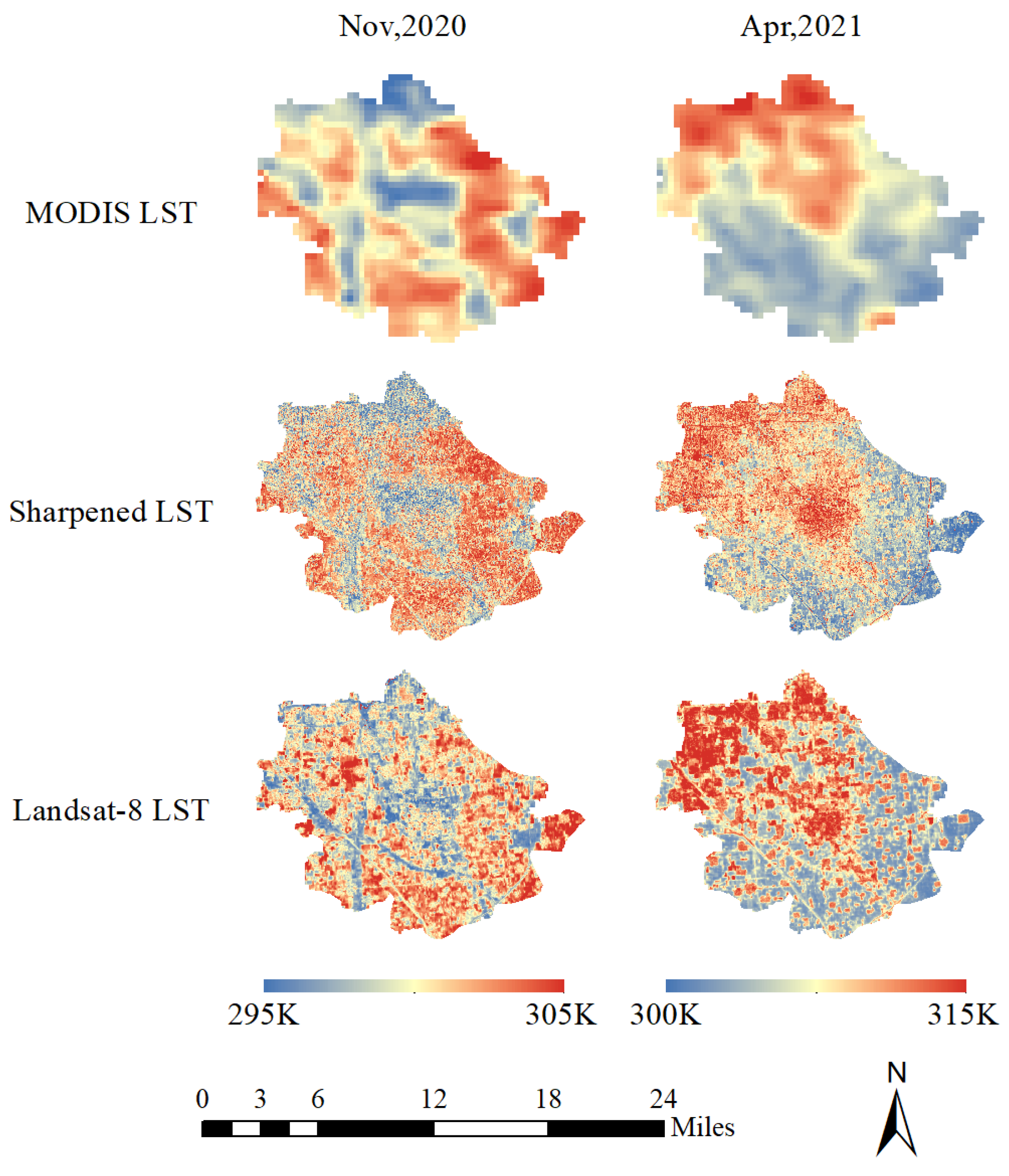
The sharpening performance of LST in different periods was compared and validated against Landsat-derived LST. As shown in Figure 5, the adopted LST sharpening model can effectively enhance the spatial resolution of MODIS LST products and yields LST values that agree well with Landsat retrievals. Nevertheless, the sharpened results exhibit moderate smoothing and attenuation of extreme values, accompanied by weaker spatial heterogeneity relative to Landsat LST. This problem originates from the coarse spatial resolution of original MODIS LST data, which leads to severe pixel mixing and inherent smoothing of extreme LST values, together with limited extrapolation capability of the sharpening model.

4.3. Evaluation of the Results and Accuracy of Space-Time Fusion

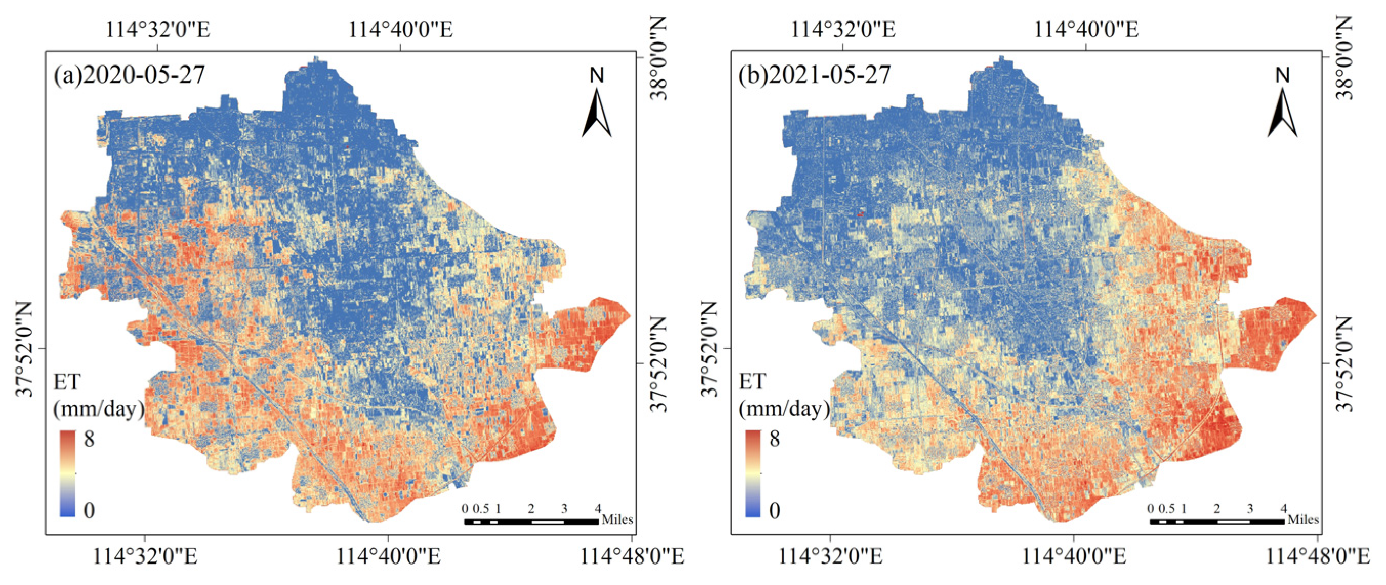
The ET results retrieved based on Sentinel-2 data and sharpened LST are shown in Figure 6. The ET values of winter wheat are mainly concentrated in the range of 4–8 mm/day. High-ET areas are distributed in the eastern and southern parts of the study region, while ET in the western area decreased in 2021 compared with 2020. Overall, although sharpened land surface temperature can provide richer spatial details for ET calculation, due to the limitations of sharpening performance, ET differences over regions with complex land cover types (e.g., farmlands surrounding built-up areas) are smoothed to a certain extent.

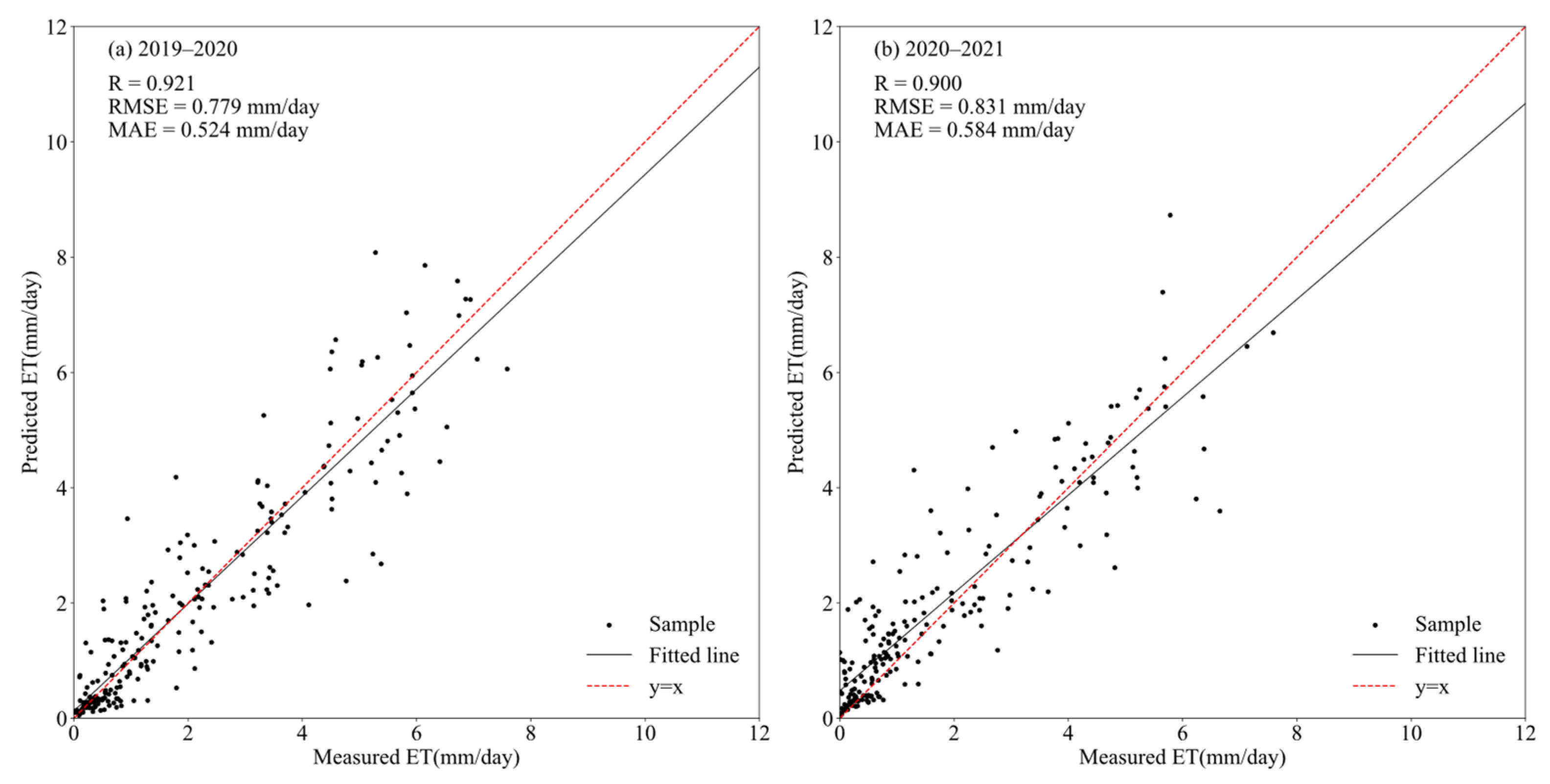
Predicted ET at the Luancheng flux station was validated against in situ measured ET observations from 2019 to 2021, and the validation results are presented in Figure 7. For 2019–2020 daily ET validation, the correlation coefficient R = 0.921, RMSE = 0.779 mm/day, and MAE = 0.524 mm/day, indicating good consistency between predicted and field-measured values. Owing to the shortage of high-resolution remote sensing images during 2020–2021, the prediction accuracy of daily ET slightly declined compared with the previous period, with R = 0.900, RMSE = 0.831 mm/day, and MAE = 0.584 mm/day, respectively. Overall, the daily ET dataset generated via spatiotemporal fusion of evapotranspiration combined with reference evapotranspiration interpolation achieves satisfactory accuracy, which proves that the high-spatiotemporal-resolution ET derived from this method is practically applicable.

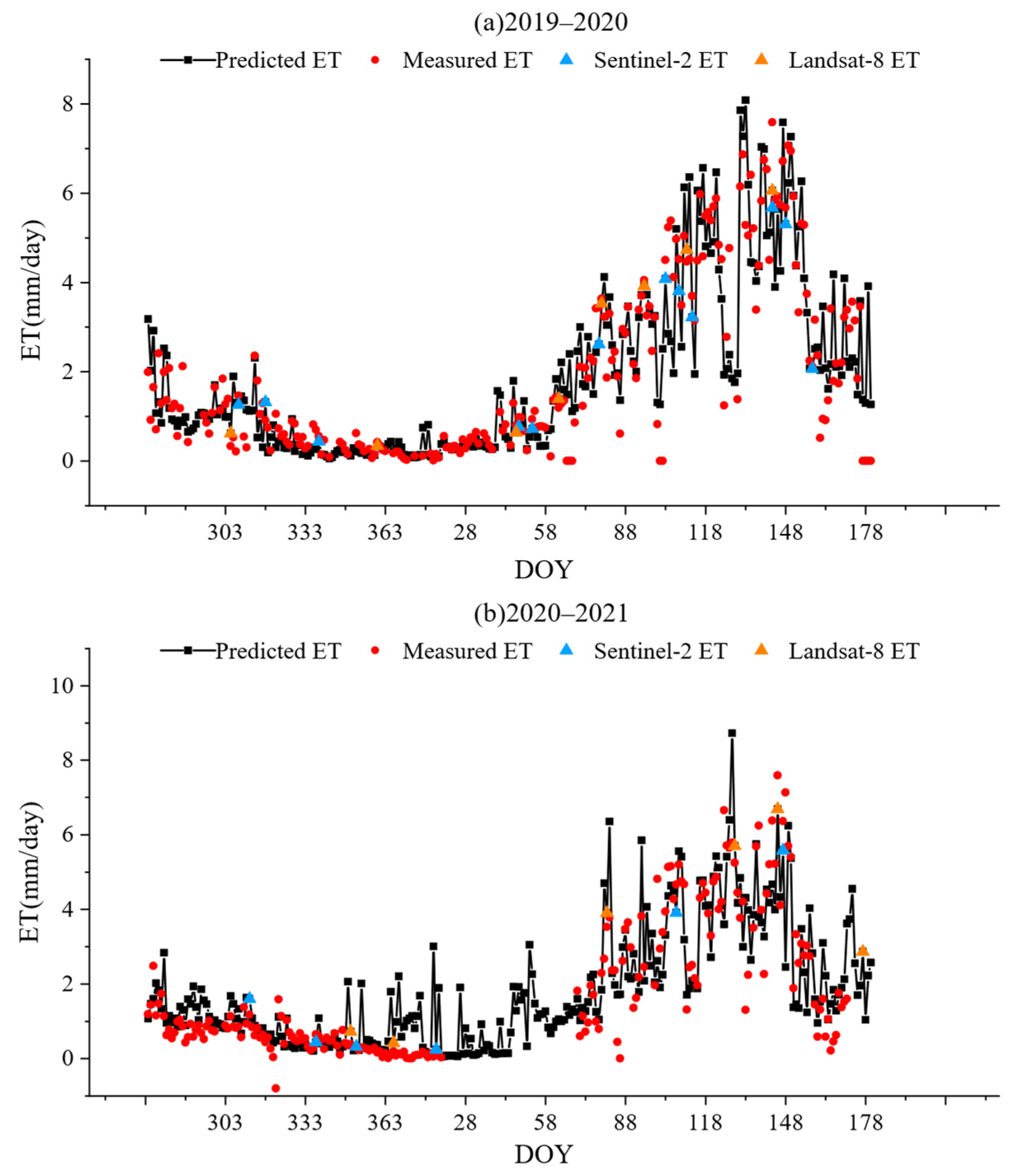
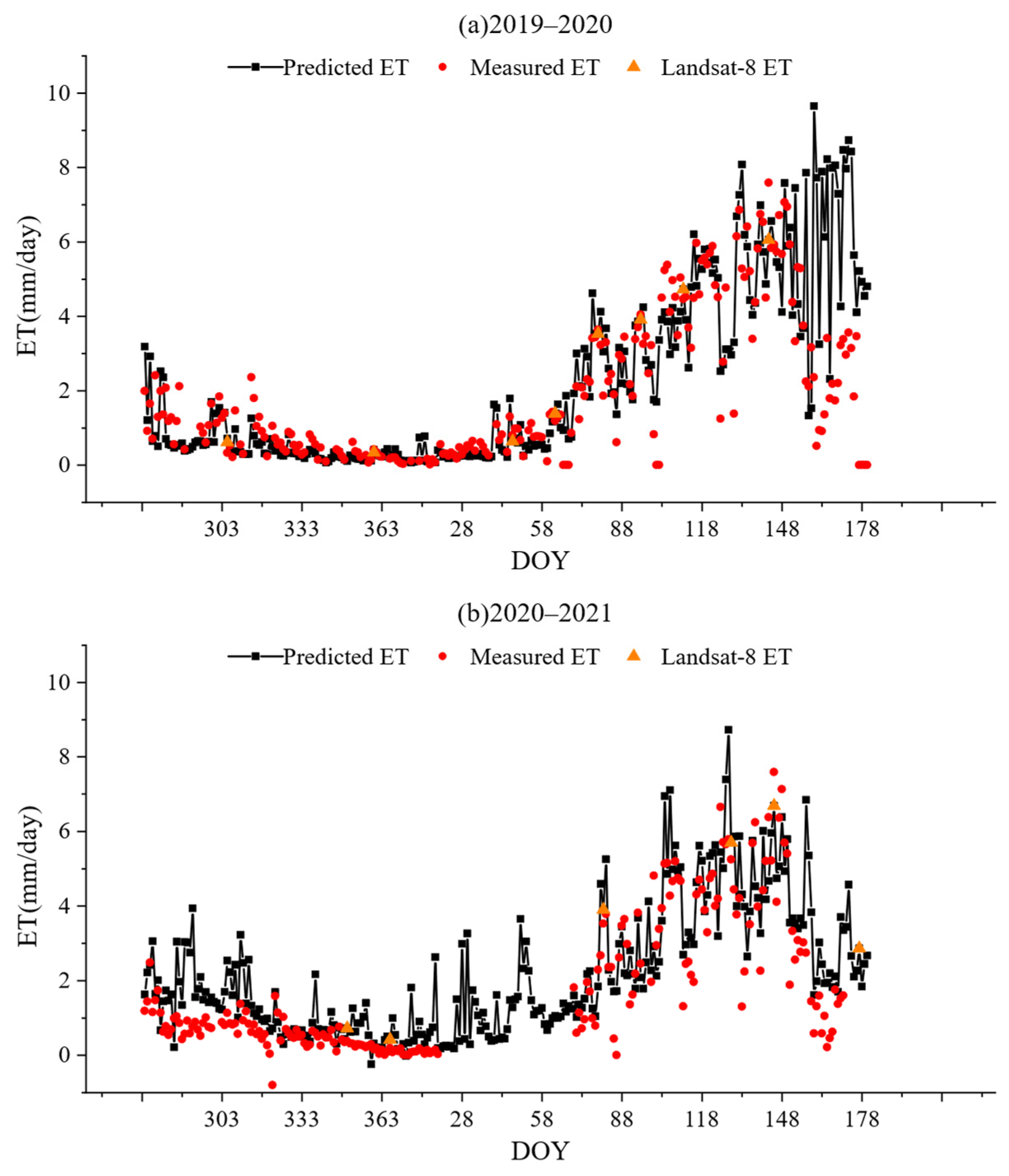
The temporal variations in predicted daily ET at the Luancheng flux station were compared with measured ET from 2019 to 2021, and the comparison results are shown in Figure 8. The predicted ET exhibits good temporal consistency with in situ observations during 2019–2020 and successfully captures short-term ET fluctuations, specifically from DOY 88 to DOY 118 and DOY 133 to DOY 153 in 2020. Despite partial gaps in the measured data caused by equipment malfunctions in 2020–2021, the overall predicted values remain in reasonable agreement with field observations.

5. Discussion

5.1. Impacts of Auxiliary Variables and LST Sharpening on ET Retrieval

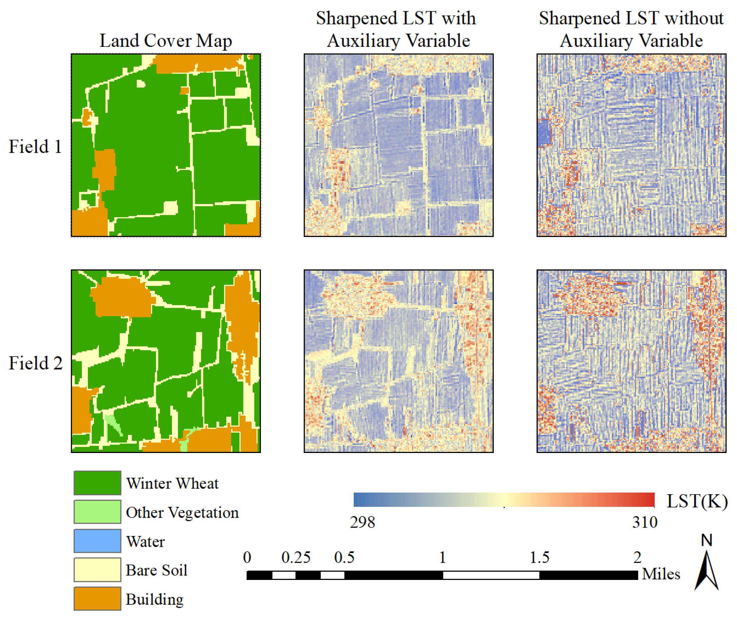
Figure 9 presents the sharpened LST results for the local area, before and after introducing auxiliary variables. When only surface reflectance is adopted as the input for the Cubist model, the sharpened outputs fail to characterize actual variations in land cover types. Surface reflectance inherently fluctuates over a certain spatial range; hence, LST retrieved merely from reflectance variations lacks fine spatial details and can only capture overall changing trends. Such results deviate from physical principles and hinder refined evapotranspiration estimation over winter wheat fields in subsequent analysis. After incorporating auxiliary variables including land cover type, the refined LST results distinctly delineate spatial details and land object boundaries. Low-temperature zones are concentrated in winter wheat areas, while high temperatures correspond to surrounding built-up lands and bare soils, making the spatial pattern of sharpened LST more physically reasonable.

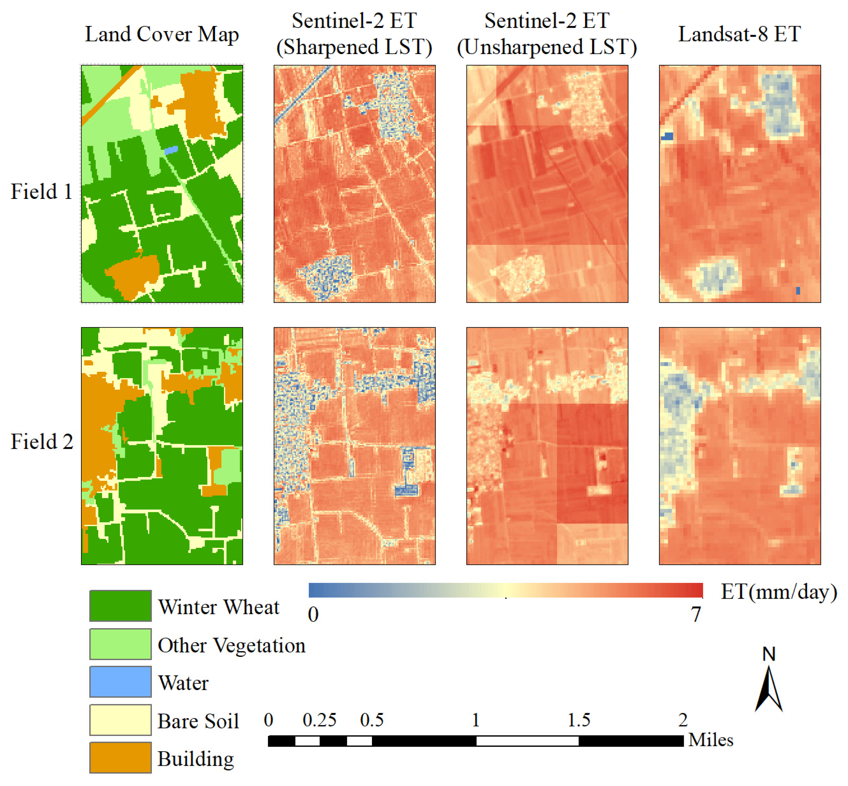
To investigate the effect of LST sharpening on ET estimation, the original coarse-resolution LST was simply resampled to 10 m resolution to calculate Sentinel-2-based ET, which was further compared with the ET derived from sharpened LST. As shown in Figure 10, ET predicted from unsharpened LST inherits artificial box-like discontinuities inherent to coarse-resolution LST and presents poor spatial heterogeneity, failing to effectively distinguish ET discrepancies across diverse land cover types. In contrast, ET computed using sharpened LST reveals abundant fine spatial details: low ET values correspond to building areas, whereas high ET concentrates within winter wheat fields. Compared with ET from unsharpened LST, this improved spatial pattern matches the actual land cover distribution better and achieves favorable consistency with Landsat-8-derived ET products.

5.2. Comparison of Spatiotemporal Fusion Effects Before and After the Introduction of Sentinel-2 ET

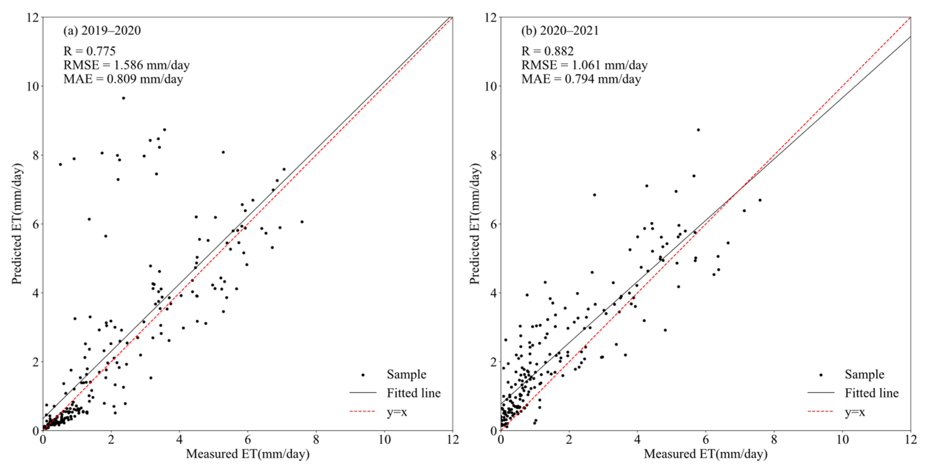
To quantify the improvement in the accuracy of high-spatiotemporal-resolution ET from incorporating Sentinel-2-derived ET, daily ET across the study area was retrieved solely using Landsat-8 ET as the input in the spatiotemporal fusion model. Accuracy assessment was implemented following the aforementioned verification procedure, and the outcomes were compared against the previous validation results. Figure 11 displays the daily ET validation statistics at the flux site. For 2019–2020, the correlation coefficient R was only 0.775, with RMSE = 1.586 mm/day and MAE = 0.809 mm/day; all three metrics indicated inferior accuracy relative to the ET dataset integrated with Sentinel-2 data. In terms of data distribution, although most validation points scatter evenly alongside the y = x reference line, partial ET values are substantially overestimated. This bias is mainly attributed to the limited temporal coverage of pure Landsat-8/9 observations, which restricts fusion performance during periods with drastic ET fluctuations. In 2020–2021, R reached 0.882 alongside RMSE = 1.061 mm/day and MAE = 0.794 mm/day. Despite marginally better performance than the 2019–2020 period, the accuracy remains lower than that of the Sentinel-2-incorporated ET product. In addition to the overestimation of several low measured ET values, more outliers are detected, further degrading the overall simulation accuracy.

Temporal comparison is illustrated in Figure 12. Restricted by limited available Landsat-8 observations, high-resolution ET fails to fully cover all growth stages of winter wheat. For 2019–2020, although predicted ET generally agrees with in situ measurements, an obvious deviation emerges from DOY 148 to DOY 181 when winter wheat is fully harvested, and field-observed ET drops to 1–4 mm/day. Owing to the absence of Landsat-8/9 ET references in this window, modeled daily ET fluctuates between 3 and 8 mm/day and diverges from actual field conditions. The number of valid Landsat-8 scenes further decreases in 2020–2021; for instance, no usable Landsat-8 data exists before DOY 347 in 2020, leading to remarkably overestimated daily ET and increased outliers throughout the crop growing season.

Overall, daily ET derived exclusively from Landsat-8 shows poorer temporal consistency with ground measurements compared with the ET integrated with Sentinel-2 data, with prominent accuracy degradation during periods suffering severe Landsat data shortage. By comparing two pairs of figures—Figure 7 with Figure 11, and Figure 8 with Figure 12, Sentinel-2 observations effectively fill temporal gaps of Landsat-8 and provide continuous high-resolution coverage across all phenological phases of winter wheat. The increased amount of fine-resolution ET inputs optimizes spatiotemporal fusion performance and contributes substantially to accuracy improvement of final ET estimations.

6. Conclusions

This study proposes an ET retrieval method based on LST sharpening. This method uses the LST sharpening model to sharpen the coarse MODIS LST down to 10 m. MODIS LST is used to address the deficiency of thermal infrared bands onboard Sentinel-2. The method also integrates a training regression tree model to improve MODIS LST. Daily ET values are further computed from Sentinel-2, Landsat-8, and MODIS datasets, and a spatiotemporal ET fusion model is adopted to generate daily 10 m ET maps covering the whole winter wheat growing season across the study area.

Incorporation of auxiliary variables improves the physical rationality and spatial details of MODIS LST products. DEM, NDVI, and land cover data exhibit high importance contributions in the regression model and enrich fine spatial features within sharpened outputs. Additionally, daily predicted ET at the Luancheng flux station was validated against in situ measured ET observations from 2019 to 2021, and the R varied from 0.775 to 0.921, the RMSE from 1.586 to 0.779, and the MAE from 0.809 to 0.524 in 2019–2020, and the R varied from 0.882 to 0.900, the RMSE from 1.061 to 0.831, the MAE from 0.794 to 0.584 before and after the introduction of Sentinel-2 ET. It also has good temporal consistency with in situ observations during 2019–2021. It is certified that Sentinel-2 data effectively fill temporal gaps caused by insufficient Landsat observations during fusion; The increased quantity of high-resolution inputs ultimately elevates the accuracy of spatiotemporal fused ET results.

It should be noted that this study conducted inversion and validation in only one agricultural district, and due to limited validation data, the accuracy of LST sharpening was not further verified. Therefore, further investigation is still needed to evaluate the generalizability of the proposed method across different regions and under diverse environmental conditions, as well as the reliability of the LST sharpening process.

References

1. Pereira, L.S.; Perrier, A.; Allen, R.G.; Alves, I. Evapotranspiration: Concepts and future trends. J. Irrig. Drain. Eng. 1999, 125, 45–51. [Google Scholar] [CrossRef] [Scilit]
2. Zhang, X.; Wu, J.; Wu, H.; Chen, H.; Zhang, T. Improving temporal extrapolation for daily evapotranspiration using radiation measurements. J. Appl. Remote Sens. 2013, 7, 073538. [Google Scholar] [CrossRef] [Scilit]
3. Silva, I.W.; Marques, T.V.; Urbano, S.A.; Mendes, K.R.; Oliveira, A.C.C.; Nascimento, F.D.S.; de Morais, L.F.; Pereira, W.D.S.; Mutti, P.R.; Neto, J.V.E.; et al. Meteorological and biophysical controls of evapotranspiration in tropical grazed pasture under rainfed conditions. Agric. Water Manag. 2024, 299, 108884. [Google Scholar] [CrossRef] [Scilit]
4. Zhang, K.; Kimball, J.S.; Running, S.W. A review of remote sensing based actual evapotranspiration estimation. Wiley Interdiscip. Rev. Water 2016, 3, 834–853. [Google Scholar] [CrossRef] [Scilit]
5. Kustas, W.P.; Norman, J.M. Use of remote sensing for evapotranspiration monitoring over land surfaces. Hydrol. Sci. J. 1996, 41, 495–516. [Google Scholar] [CrossRef] [Scilit]
6. Guo, X.; Meng, D.; Chen, X.; Li, X. Validation and Comparison of Seven Land Surface Evapotranspiration Products in the Haihe River Basin, China. Remote Sens. 2022, 14, 4308. [Google Scholar] [CrossRef] [Scilit]
7. Awada, H.; Di Prima, S.; Sirca, C.; Giadrossich, F.; Marras, S.; Spano, D.; Pirastru, M. A remote sensing and modeling integrated approach for constructing continuous time series of daily actual evapotranspiration. Agric. Water Manag. 2022, 260, 107320. [Google Scholar] [CrossRef] [Scilit]
8. Tran, B.N.; Van Der Kwast, J.; Seyoum, S.; Uijlenhoet, R.; Jewitt, G.; Mul, M. Uncertainty assessment of satellite remote-sensing-based evapotranspiration estimates: A systematic review of methods and gaps. Hydrol. Earth Syst. Sci. 2023, 27, 4505–4528. [Google Scholar] [CrossRef] [Scilit]
9. Zhu, P.; Han, Q.; Li, S.; Liu, H.; Li, C.; Ma, Y.; Wang, J. A Novel Framework Based on Data Fusion and Machine Learning for Upscaling Evapotranspiration from Flux Towers to the Regional Scale. Remote Sens. 2025, 17, 3813. [Google Scholar] [CrossRef] [Scilit]
10. Gao, F.; Masek, J.; Schwaller, M.; Hall, F. On the Blending of the Landsat and MODIS Surface Reflectance: Predicting Daily Landsat Surface Reflectance. IEEE Trans. Geosci. Remote Sens. 2006, 44, 2207–2218. [Google Scholar] [CrossRef] [Scilit]
11. Zhu, X.; Chen, J.; Gao, F.; Chen, X.; Masek, J.G. An enhanced spatial and temporal adaptive reflectance fusion model for complex heterogeneous regions. Remote Sens. Environ. 2010, 114, 2610–2623. [Google Scholar] [CrossRef] [Scilit]
12. Zhang, X.; Gao, H.; Shi, L.; Hu, X.; Zhong, L.; Bian, J. Mapping crop evapotranspiration by combining the unmixing and weight image fusion methods. Remote Sens. 2024, 16, 2414. [Google Scholar] [CrossRef] [Scilit]
13. Alfieri, J.G.; Anderson, M.C.; Kustas, W.P.; Cammalleri, C. Effect of the revisit interval and temporal upscaling methods on the accuracy of remotely sensed evapotranspiration estimates. Hydrol. Earth Syst. Sci. 2017, 21, 83–98. [Google Scholar] [CrossRef] [Scilit]
14. Zhu, X.; Helmer, E.H.; Gao, F.; Liu, D.; Chen, J.; Lefsky, M.A. A flexible spatiotemporal method for fusing satellite images with different resolutions. Remote Sens. Environ. 2016, 172, 165–177. [Google Scholar] [CrossRef] [Scilit]
15. Guillevic, P.; Olioso, A.; Hook, S.; Fisher, J.B.; Lagouarde, J.-P.; Vermote, E.F. Impact of the Revisit of Thermal Infrared Remote Sensing Observations on Evapotranspiration Uncertainty—A Sensitivity Study Using AmeriFlux Data. Remote Sens. 2019, 11, 573. [Google Scholar] [CrossRef] [Scilit]
16. Crow, W.T.; Anderson, M.C.; Volk, J.M.; Colliander, A. Value of microwave soil moisture and thermal-infrared evapotranspiration retrievals for the mapping of irrigation coverage. Int. J. Appl. Earth Obs. Geoinf. 2025, 143, 104773. [Google Scholar] [CrossRef] [Scilit]
17. Tang, Y.; Zhao, Y.; Sun, Y.; Ren, S.; Li, Z. Seamless Reconstruction of MODIS Land Surface Temperature via Multi-Source Data Fusion and Multi-Stage Optimization. Remote Sens. 2025, 17, 3374. [Google Scholar] [CrossRef] [Scilit]
18. Wang, Z.; Zhang, Y.L.; Zhang, Q.C.; Li, Z.L. Validation of the land surface temperature products retrieved from Terra Moderate Resolution Imaging Spectrometer data. Remote Sens. Environ. 2002, 83, 163–180. [Google Scholar] [CrossRef] [Scilit]
19. Fu, P.; Xie, Y.; Weng, Q.; Myint, S.; Meacham-Hensold, K.; Bernacchi, C. A Physical Model-Based Method for Retrieving Urban Land Surface Temperatures under Cloudy Conditions. Remote Sens. Environ. 2019, 230, 111191. [Google Scholar] [CrossRef] [Scilit]
20. Kustas, W.P.; Norman, J.M.; Anderson, M.C.; French, A.N. Estimating subpixel surface temperatures and energy fluxes from the vegetation index–radiometric temperature relationship. Remote Sens. Environ. 2003, 85, 429–440. [Google Scholar] [CrossRef] [Scilit]
21. Agam, N.; Kustas, W.P.; Anderson, M.C.; Li, F.; Neale, C.M. A vegetation index based technique for spatial sharpening of thermal imagery. Remote Sens. Environ. 2007, 107, 545–558. [Google Scholar] [CrossRef] [Scilit]
22. Gao, F.; Kustas, W.P.; Anderson, M.C. A Data Mining Approach for Sharpening Thermal Satellite Imagery over Land. Remote Sens. 2012, 4, 3287–3319. [Google Scholar] [CrossRef] [Scilit]
23. Guzinski, R.; Nieto, H. Evaluating the feasibility of using Sentinel-2 and Sentinel-3 satellites for high-resolution evapotranspiration estimations. Remote Sens. Environ. 2019, 221, 157–172. [Google Scholar] [CrossRef] [Scilit]
24. Guzinski, R.; Nieto, H.; Sandholt, I.; Karamitilios, G. Modelling High-Resolution Actual Evapotranspiration through Sentinel-2 and Sentinel-3 Data Fusion. Remote Sens. 2020, 12, 1433. [Google Scholar] [CrossRef] [Scilit]
25. Guzinski, R.; Nieto, H.; Sánchez, R.R.; Sánchez, J.M.; Jomaa, I.; Zitouna-Chebbi, R.; Roupsard, O.; López-Urrea, R. Improving field-scale crop actual evapotranspiration monitoring with Sentinel-3, Sentinel-2, and Landsat data fusion. Int. J. Appl. Earth Obs. Geoinf. 2023, 125, 103587. [Google Scholar] [CrossRef] [Scilit]
26. Liu, F.; Shen, Y.; Cao, J.; Zhang, Y. A dataset of water, heat, and carbon fluxes over the winter wheat-summer maize croplands in Luancheng during 2013–2017. China Sci. Data 2023, 8, 1–10. [Google Scholar] [CrossRef] [Scilit]
27. Blaschke, T. Object based image analysis for remote sensing. ISPRS J. Photogramm. Remote Sens. 2010, 65, 2–16. [Google Scholar] [CrossRef] [Scilit]
28. Meng, X.; Zeng, J.; Yang, Y.; Zhao, W.; Ma, H.; Letu, H.; Zhu, Q.; Liu, Y.; Wang, P.; Peng, J. High-resolution soil moisture mapping through passive microwave remote sensing downscaling. Innov. Geosci. 2024, 2, 100105. [Google Scholar] [CrossRef] [Scilit]
29. Quinlan, J.R. Learning with Continuous Classes. In Proceedings of 5th Australian Joint Conference on Artificial Intelligence, Hobart, Tasmania, 16–18 November 1992; World Scientific Publishing: Singapore, 1992; pp. 343–348. [Google Scholar]
30. Quinlan, J.R. Rulequest Data Mining Tools. Available online: http://www.rulequest.com/ (accessed on 10 October 2024).
31. Myers, W.N.C. A data mining approach to soil temperature and moisture prediction. In Proceedings of the Seventh Conference on Artificial Intelligence and Its Applications to the Environmental Sciences, Phoenix, AZ, USA, 13 January 2009. [Google Scholar]
32. Allen, R.; Irmak, A.; Trezza, R.; Hendrickx, J.M.H.; Bastiaanssen, W.; Kjaersgaard, J. Satellite-based ET estimation in agriculture using SEBAL and METRIC. Hydrol. Process. 2011, 25, 4011–4027. [Google Scholar] [CrossRef] [Scilit]
33. Norman, J.M.; Kustas, W.P.; Humes, K.S. Source approach for estimating soil and vegetation energy fluxes in observations of directional radiometric surface temperature. Agric. For. Meteorol. 1995, 77, 263–293. [Google Scholar] [CrossRef] [Scilit]
34. Allen, R.G.; Tasumi, M.; Trezza, R. Satellite-Based Energy Balance for Mapping Evapotranspiration with Internalized Calibration (METRIC)—Model. J. Irrig. Drain. Eng. 2007, 133, 380–394. [Google Scholar] [CrossRef] [Scilit]
35. Han, L.; Gao, F.; Dong, S.; Song, Y.; Liu, H.; Song, N. Simulating Daily Evapotranspiration of Summer Soybean in the North China Plain Using Four Machine Learning Models. Agronomy 2026, 16, 315. [Google Scholar] [CrossRef] [Scilit]
36. Acharya, B.; Sharma, V. Comparison of satellite driven surface energy balance models in estimating crop evapotranspiration in semi-arid to arid inter-mountain region. Remote Sens. 2021, 13, 1822. [Google Scholar] [CrossRef] [Scilit]
37. Claudino, C.M.A.; Bertrand, G.F.; Nóbrega, R.L.B.; Almeida, C.D.N.; Gusmão, A.C.V.; Montenegro, S.M.; Silva, B.B.; Patriota, E.G.; Lemos, F.C.; Coutinho, J.V.; et al. ESTIMET: Enhanced and Spatial-Temporal Improvement of MODIS EvapoTranspiration algorithm for all sky conditions in tropical biomes. Remote Sens. Environ. 2025, 325, 114771. [Google Scholar] [CrossRef] [Scilit]
38. Bastiaanssen, W.G.M.; Pelgrum, H.; Wang, J.; Ma, Y.; Moreno, J.F.; Roerink, G.J.; van der Wal, T. A remote sensing surface energy balance algorithm for land (SEBAL). J. Hydrol. 1998, 212, 198–212. [Google Scholar] [CrossRef] [Scilit]
39. Van De Griend, A.A.; Owe, M. On the relationship between thermal emissivity and the normalized difference vegetation index for natural surfaces. Int. J. Remote Sens. 1993, 14, 1119–1131. [Google Scholar] [CrossRef] [Scilit]
40. Gao, H.; Zhang, X.; Wang, X.; Zeng, Y. Phenology-Based Remote Sensing Assessment of Crop Water Productivity. Water 2023, 15, 329. [Google Scholar] [CrossRef] [Scilit]
41. Liang, S.L. Narrowband to broadband conversions of land surface albedo I Algorithms. Remote Sens. Environ. 2001, 76, 213–238. [Google Scholar] [CrossRef] [Scilit]
42. Naegeli, K.; Damm, A.; Huss, M.; Wulf, H.; Schaepman, M.; Hoelzle, M. Cross-Comparison of Albedo Products for Glacier Surfaces Derived from Airborne and Satellite (Sentinel-2 and Landsat 8) Optical Data. Remote Sens. 2017, 9, 110. [Google Scholar] [CrossRef] [Scilit]
43. Zhukov, B.; Oertel, D.; Lanzl, F.; Reinhackel, G. Unmixing-based multisensor multiresolution image fusion. IEEE Trans. Geosci. Remote Sens. 1999, 37, 1212–1226. [Google Scholar] [CrossRef] [Scilit]
44. Allan, R.; Pereira, L.; Smith, M. Crop Evapotranspiration-Guidelines for Computing Crop Water Requirements; FAO Irrigation and Drainage Paper 56; FAO: Rome, Italy, 1998. [Google Scholar]
45. Monteith, J.L. Evaporation and environment. In Symposia of the Society for Experimental Biology; Cambridge University Press: Cambridge, UK, 1965; Volume 19, pp. 205–234. [Google Scholar]
46. Priestley, C.H.B.; Taylor, R.J. On the assessment of surface heat flux and evaporation using large-scale parameters. Mon. Weather Rev. 1972, 100, 81–92. [Google Scholar] [CrossRef] [Scilit]
47. Talsma, C.J.; Good, S.P.; Jimenez, C.; Martens, B.; Fisher, J.B.; Miralles, D.G.; McCabe, M.F.; Purdy, A.J. Partitioning of evapotranspiration in remote sensing-based models. Agric. For. Meteorol. 2018, 260, 131–143. [Google Scholar] [CrossRef] [Scilit]
Figure 1. Location of Luancheng.
Remotesensing 18 03039 g001
Figure 2. Land cover map of Luancheng. (a) 2019–2020; (b) 2020–2021.
Remotesensing 18 03039 g002
Figure 3. The overall workflow.
Remotesensing 18 03039 g003
Figure 4. The workflow of the LST sharpening model.
Remotesensing 18 03039 g004
Figure 5. Spatial distribution of LST.
Remotesensing 18 03039 g005
Figure 6. ET retrieved from Sentinel-2 data and sharpened LST. (a) 27 May 2020; (b) 27 May 2021.
Remotesensing 18 03039 g006
Figure 7. Accuracy validation of daily ET for winter wheat at the flux station. (a) 2019–2020; (b) 2020–2021.
Remotesensing 18 03039 g007
Figure 8. Comparison of daily winter wheat ET against flux measurements. (a) 2019–2020; (b) 2020–2021.
Remotesensing 18 03039 g008
Figure 9. Influence of auxiliary variables in the LST sharpening model.
Remotesensing 18 03039 g009
Figure 10. Influence of LST sharpening on Sentinel-2 ET.
Remotesensing 18 03039 g010
Figure 11. Accuracy validation of daily ET for winter wheat at the flux station using solely Landsat-8 ET as the input in the spatiotemporal fusion model. (a) 2019–2020; (b) 2020–2021.
Remotesensing 18 03039 g011
Figure 12. Comparison of daily winter wheat ET against flux measurements using solely Landsat-8 ET as the input in the spatiotemporal fusion model. (a) 2019–2020; (b) 2020–2021.
Remotesensing 18 03039 g012