Satellite–UAV Collaborative Off-Road Traversability Mapping and Incremental Updating for Unmanned Ground Vehicles

Highlights

What are the main findings?

• A three-layer off-road traversability map connects heterogeneous regional evidence to planner-ready costs through a common H3 spatial index.
• A fixed-grid, observer-agnostic UAV workflow revises local semantic states and costs without reconstructing the regional prior.

What are the implications of the main findings?

• UAV override preserves global map coverage while limiting the false-positive accumulation caused by within-footprint prior union.
• Hard and finite risk costs reveal a transparent trade-off between reference-risk avoidance and search-graph connectivity.

Abstract

Large-area remote-sensing data provide essential pre-mission information for unmanned ground vehicles, but their spatial support and temporal latency may obscure local terrain changes. A remaining challenge is to translate heterogeneous regional evidence and recent local observations into a consistent, updateable, and planner-ready map. This study presents a satellite–unmanned aerial vehicle (UAV) workflow for constructing and incrementally maintaining an off-road traversability map for mission-level global planning. A common H3 index organizes satellite imagery, terrain, soil, road evidence, and local UAV semantic observations while retaining their native spatial support and provenance. The map separates environmental-prior, semantic, and traversability-cost layers to support interpretable fusion and independent updating. A confidence-hierarchical conflict resolution mechanism resolves inconsistencies in the regional prior, while an observer-agnostic interface projects UAV semantic observations onto local map cells. RGB imagery is used by the primary UAV observer, and digital surface model (DSM) is evaluated as an optional semantic-observation modality. Evaluation included a manually reviewed regional benchmark, a unified buffered spatial holdout, cell-level update assessment, and 40 fixed replanning tasks. Conflict resolution reduced high-risk omissions. RGB-only SegFormer-B2 achieved the highest semantic accuracy with moderate computational complexity. UAV override achieved a cell-level F1 score of 96.96% and limited the false-positive accumulation associated with conservative union. Replanning further revealed a trade-off between hazardous-cell avoidance and search-graph connectivity. The proposed workflow provides a maintainable interface between multi-source remote sensing and global UGV planning rather than a replacement for onboard perception, local obstacle avoidance, or vehicle control.

1. Introduction

Unmanned ground vehicles (UGVs) are increasingly considered for operations in unstructured environments, including agriculture, rescue, exploration, and other field missions [1]. Multimodal fusion has also been investigated for end-to-end UGV trajectory prediction [2]. Compared with structured urban roads, roadless and off-road environments such as forests, farmland, mountainous terrain, riverbanks, and post-disaster areas often lack predefined paths and persistent lane-level cues. Their large spatial extent and environmental variability make complete pre-mission navigation-map construction difficult [3]. Onboard sensing remains essential for near-field obstacle avoidance, but the vehicle also needs a regional estimate of feasible traversal, concentrated planning risk, and excluded areas before local perception becomes available. A prior traversability map therefore provides mission-level context for global path planning.

The map representation required for urban autonomous driving differs markedly from that required for off-road UGV navigation. High-definition maps in urban scenarios are typically designed for structured road traffic and mainly represent lane markings, road boundaries, traffic signs, traffic signals, road topology, and high-precision localization elements [4]. Their primary purpose is to support lane-level localization, behavior decision-making, and path tracking within existing road networks. In contrast, the primary question for an off-road UGV is not how to follow an existing road but where traversal is feasible and at what estimated cost. Abrupt slope changes, loose surfaces, vegetation occlusion, water blockage, road damage, and isolated obstacles may constrain mobility through terrain, soil, land-cover, and vehicle-dynamic factors [5,6]. Off-road traversability maps therefore should not simply inherit the representation logic of urban high-definition maps. Instead, they should transform terrain geometry, land cover, soil conditions, hydrological risk, and discrete obstacles into vehicle-interpretable traversability states and planning costs.

Existing mobile-robot mapping methods provide an important foundation for unmanned vehicle navigation. Occupancy grids represent cell occupancy probabilistically and support incremental updates from sensor observations [7], while grid-based cost and elevation maps provide convenient local representations for navigation over uneven terrain [8]. These representations are effective for obstacle-centric mapping and local planning, but occupancy alone does not express many factors that determine off-road mobility. Slope, terrain roughness, surface type, deformable or wet soil, vegetation, and vehicle–terrain interaction often require additional terrain layers or explicit traversability-cost models [1,5,6]. A large-area off-road map should therefore describe not only where obstacles are located but also the source and degree of estimated traversal risk and how that estimate changes when new observations arrive.

Satellite and UAV remote sensing provide complementary data sources for constructing such task-oriented traversability maps. Sentinel-2-based products can provide frequently updated large-area land-cover information [9]. Global elevation products provide regional terrain geometry; newer bare-earth products such as FABDEM reduce building and forest-height biases while retaining approximately 30 m global coverage [10]. Soil properties and moisture-related information can inform soil-strength and vehicle-trafficability estimation [11]. In the present study, however, these regional products are treated as susceptibility evidence rather than as direct measurements of sinkage or slip. Road patterns can be extracted from remote-sensing imagery [12], while OpenStreetMap (OSM) can provide an auxiliary road-network prior for global route generation [13]. These sources are complementary, but they are not geometrically or temporally interchangeable. Differences in spatial resolution, acquisition time, sensing mechanism, orthorectification, and co-registration can propagate into the fused map if they are not handled explicitly [14]. The problem becomes more acute after disasters, when road accessibility may change as new disruptions are discovered [15]. Remote-sensing change detection can identify differences between observations acquired at different times [16]. For UGV planning, these detected changes must subsequently be translated into vehicle-relevant traversability states and costs.

Unmanned aerial vehicle (UAV) remote sensing offers high spatial resolution, flexible low-altitude deployment, and rapid data acquisition, enabling detailed local observations of selected areas and providing an important source for the updating of large-scale prior traversability maps [17]. Recent RTK-assisted photogrammetry studies have reported centimeter-level direct-georeferencing accuracy under appropriate configurations [18], and work on complex topography has shown that flight geometry, image orientation, georeferencing strategy, and ground sampling distance materially affect the accuracy of UAV-derived elevation models [19]. This spatial accuracy is important when small terrain discontinuities or narrow obstacles are projected into a global planning grid. RGB and DSM can provide complementary appearance and surface-height cues for multimodal remote-sensing segmentation [20], and boundary-aware fusion has improved elevation-discontinuity and fine-structure recovery in some datasets [21]. Such gains are nevertheless contingent on DSM quality, cross-modal registration, fusion design, and target data; they are therefore tested rather than assumed in this study. A UAV flight covers only a local footprint. Rebuilding the entire regional map after each flight would be inefficient, while a binary change mask does not, by itself, provide an updated planning cost. The practical problem is therefore how to write local, high-resolution UAV observations back into a large-scale prior map without losing spatial consistency or suppressing newly observed high-risk changes.

To address this integration gap, this study develops a satellite–UAV workflow that connects regional prior-map construction, local semantic observation, incremental map maintenance, and global replanning. The main contributions are described as follows:

(1)

A provenance-preserving representation of the off-road traversability map is developed using a common H3 spatial index. The map separates environmental-prior, semantic, and traversability-cost layers, allowing heterogeneous evidence to be aggregated and updated without obscuring its original source or spatial support. The evaluated implementation uses fixed H3-12 cells for the regional prior and fixed H3-13 cells for UAV updating.

(2)

A task-oriented $C_0$–$C_4$ semantic system and an interpretable traversability-cost model are formulated for off-road global planning. The model connects land-surface semantics with bounded modifiers derived from regional slope, soil wet–soft susceptibility, and relief variability. This design converts heterogeneous environmental evidence into planner-ready costs while distinguishing regional susceptibility indicators from vehicle-scale terrain measurements.

(3)

A confidence-hierarchical conflict resolution mechanism (CHCRM) is introduced for the constructing of the regional prior. CHCRM resolves inconsistencies among satellite-derived semantics, terrain constraints, soil information, and road evidence according to physical constraints and source confidence. Its effectiveness is evaluated against a manually reviewed regional reference, with particular attention to safety-relevant high-risk omissions.

(4)

An observer-agnostic incremental updating and replanning workflow is established for local UAV observations. The workflow projects UAV semantic outputs onto fixed H3 cells and compares alternative observers, UAV override and conservative union, and hard-blocking and finite-cost policies. Their downstream effects are evaluated through cell-level map assessment and fixed global replanning tasks.

2. Related Work

Environmental maps provide the foundation for perception, planning, and decision-making in unmanned vehicles. In structured urban scenarios, HD maps emphasize high-precision road geometry, road-surface and lane elements, traffic signs and signals, and localization-relevant semantics that constrain automated driving within an existing road network [22]. Off-road environments, however, usually lack stable, continuous, and regularized road networks. For off-road UGVs, map representation must describe not only where obstacles exist but also where nominal traversal is feasible and how estimated cost varies across space. Off-road traversability maps therefore should not simply follow the urban high-definition mapping paradigm. They should represent how terrain, land cover, soil conditions, water bodies, road priors, and discrete obstacles affect vehicle mobility.

Mobile robotics have long used occupancy grids, cost maps, elevation maps, and local grid maps to represent environmental states. Occupancy grids recursively describe spatial occupancy and support local obstacle avoidance [7]. Controlled studies have also compared Bayesian and belief-function fusion for occupancy-grid mapping [23]. For rough terrain, local elevation maps accumulate geometric observations into robot-centered representations that support locomotion over uneven surfaces [24]. These approaches are effective for local navigation but are less suited to regional risks caused by slope, wet or soft soil, vegetation, ponding, and degraded road surfaces.

Off-road traversability analysis evaluates whether and at what cost a specific vehicle can negotiate unstructured terrain. Recent field-robotics research frames traversability evaluation around platform characteristics and environmental semantic and geometric features and compares methods across sensors, robot types, scenarios, and learning strategies [25]. At the regional scale, dynamic trafficability models have integrated elevation, slope, terrain position, land cover, soil, soil moisture, hazards, and meteorological factors to produce vehicle-specific maps for path planning [26]. A complementary remote-sensing inversion study estimated shallow soil moisture and soil type and coupled them with vehicle dynamics, reporting field-validated predictions of sinkage and speed for wheeled and tracked vehicles [27]. Vehicle dependence also motivates experimental validation: Eder et al. estimated robot-specific costs from locomotion experiments with four heterogeneous robots and Earth-observation terrain information [28], while Zhang et al. fused RGB semantics, point clouds, and local elevation maps and validated the resulting cost map on a Scout-2.0 UGV [29]. These studies show why map-level evidence and vehicle-level traversability validation should be distinguished explicitly.

Learning-based methods have strengthened near-field traversability estimation by combining visual, geometric, and proprioceptive cues. Self-supervised approaches can learn traversable regions from geometric and visual evidence [30], while online systems can use onboard imagery and robot interaction to adapt traversability predictions during deployment in forests, parks, and grasslands [31]. More recent visual–geometric systems combine foundation-model features with geometric mapping to produce cost, speed, and uncertainty maps and have been tested in real-world robot trials at multiple challenging off-road sites [32]. At the regional scale, remote-sensing trafficability assessment is also moving from hand-crafted rule overlays toward cross-modal learning; He et al. fused remote-sensing imagery with geographic and geological auxiliary factors and evaluated the approach on datasets from Asia and Africa [33]. These approaches have complementary strengths: onboard systems provide detailed local estimates but remain constrained by sensor range, occlusion, vehicle position, and the area that can be physically explored, whereas regional remote-sensing products can provide broader priors before vehicle deployment.

In satellite–UAV collaborative mapping, elevation resolution and spatial accuracy directly influence terrain representation and cross-platform data consistency. Because slope and elevation-variability measures are derived from elevation, vertical bias, canopy contamination, and spatial smoothing can propagate into traversability costs. FABDEM improves the bare-earth representation of global 30 m elevation data [10], while UAV-LiDAR validation in a mountainous forest shows that local terrain structure may still differ appreciably from coarse global DEMs [34]. At the observation scale, RTK UAV photogrammetry can achieve centimeter-level georeferencing under suitable conditions [18], whereas satellite products from different sensors may retain meter-scale co-registration residuals [35]. Cross-source fusion should therefore retain native spatial support and positional confidence rather than assume exact pixel correspondence.

Multi-source remote-sensing fusion for UGV navigation is therefore not equivalent to a simple overlay of map layers. Remote-sensing and geospatial sources may differ in spatial resolution, acquisition time, sensing characteristics, semantic definitions, and georegistration accuracy, creating discrepancies that must be addressed during fusion [14,36]. For example, an OSM road prior may indicate a road corridor, whereas recent imagery may show ponding or surface damage. An image classification may label an area as bare ground, while DEM-derived slope may exceed the planning threshold defined for the vehicle. Soil conditions may likewise alter the nominal cost assigned to the same land-cover class. Category overwriting, simple weighted summation, or majority voting without physical constraints can therefore produce unsuitable global routes. Traversability-oriented fusion should jointly consider land-cover semantics, terrain constraints, soil conditions, road priors, and source confidence and resolve conflicts conservatively.

The spatial organization of a traversability map affects cross-source aggregation, planning, and incremental maintenance. Regular grids remain useful because environmental attributes and planning costs can be stored cell by cell and coupled with graph-search planners [37]. In this study, H3 is selected for its globally addressable cells and direct neighborhood operations [38,39,40,41], not because the evaluated workflow performs adaptive refinement.

H3 does not, itself, solve traversability modeling or create information finer than the native sources. Its role is to provide a common carrier for multi-source evidence and local updates. Regional evidence is stored on fixed H3-12 cells, and UAV observations are projected to fixed H3-13 cells. Every record retains source resolution and provenance so that the index resolution is not confused with physical measurement support.

Regional satellite and thematic products may not capture short-term disruptions, including road damage and newly emerging obstacles, at the time required for planning [15,16]. UAV remote sensing offers flexible acquisition and high spatial detail over selected areas and is an established platform for local mapping and photogrammetric observation [42]. RGB–DSM segmentation has been reported to improve discrimination and boundary delineation when the DSM and fusion architecture provide transferable geometric cues [43]; whether this benefit persists under buffered spatial generalization is evaluated here against RGB-only models. Deep learning has expanded the available segmentation tools. U-Net established a widely used contracting–expanding architecture for dense pixel-wise prediction [44], DeepLabV3+ combines multiscale atrous context modeling with decoder-based boundary recovery [45], and SegFormer uses a hierarchical Transformer encoder and lightweight MLP decoder [46]. The Segment Anything Model (SAM) provides promptable segmentation and broad transfer across image distributions [47], while remote-sensing studies have introduced SAM-derived object and boundary constraints for semantic segmentation [48]. Parameter-efficient methods such as LoRA reduce the number of trainable parameters for downstream adaptation [49]. Focal Loss and Lovász–Softmax address different optimization needs: the former down-weights easy examples under class imbalance [50], whereas the latter is a tractable surrogate for intersection-over-union-related objectives [51].

For UGV navigation, however, UAV semantic extraction cannot stop at pixel-level land-cover classification. Conventional semantic segmentation produces class maps, while optical remote-sensing change detection compares observations of the same area acquired at different times to reveal spatiotemporal change [52]. Neither output directly determines the traversability state of an updated region, the inheritance of historical map states, the suppression of false detections from a single observation, or the trigger of path replanning. Local high-resolution observations must therefore be projected into the off-road traversability map, fused with historical states, and converted into updated costs according to estimated risk and observation confidence.

In summary, prior studies provide foundations in robotic map representation, off-road traversability analysis, multi-source remote-sensing fusion, multi-scale spatial organization, and UAV semantic segmentation. A remaining integration problem is how to construct and update a satellite–UAV collaborative off-road traversability map while preserving the support, timing, semantics, positional uncertainty, and confidence of heterogeneous sources. Existing methods usually address only part of this chain, such as occupancy representation, vehicle-specific local estimation, regional trafficability assessment, multimodal segmentation, or change detection. Their combination into an interpretable prior-map representation, conservative conflict-resolution process, and explicit update-to-replanning workflow remains insufficiently studied.

To address this integration problem, the proposed method uses H3 as a common spatial index; establishes a $C_0$–$C_4$ traversability semantic system and a multi-factor cost model; applies CHCRM to conflicts among satellite imagery, DEMs, soil attributes, and road priors; and updates the map using UAV semantic observations derived from RGB or RGB–DSM inputs, fixed H3-13 projection, validation-selected high-risk detection, and one-ring cost diffusion. The method connects remote-sensing observations to the cost layer of the off-road traversability map and evaluates the result through grid-based replanning. It does not replace onboard perception, localization, local obstacle avoidance, trajectory tracking, or vehicle-level control.

3. Methods

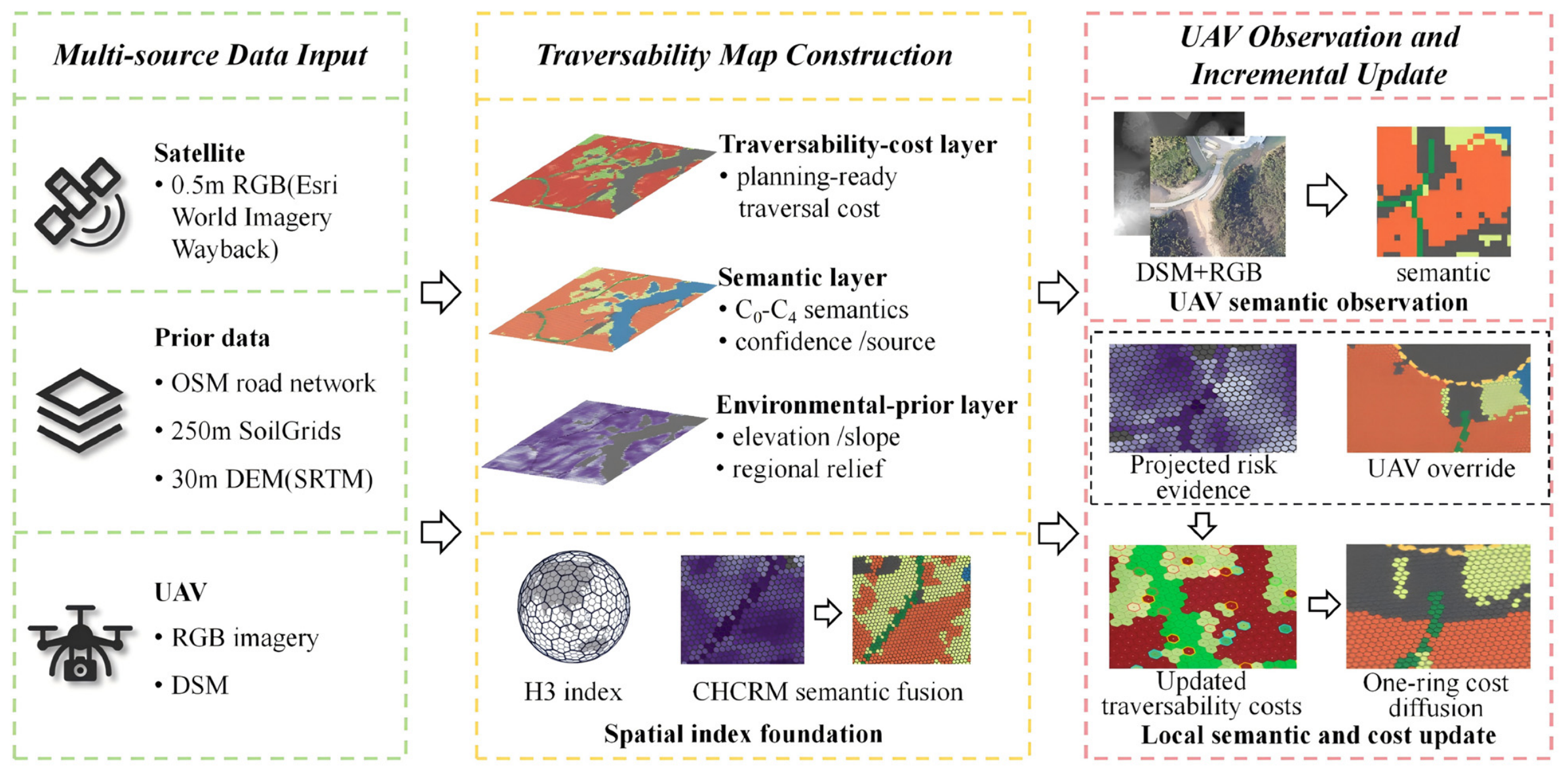
The framework constructs a regional prior state of the off-road traversability map, then updates it with UAV observations (Figure 1). A common H3 index registers all information while retaining the native spatial support of each source. Regional RGB imagery provides a $C_0$–$C_4$ semantic prior, SRTM-derived terrain attributes and SoilGrids clay content provide regional modifiers, and OSM roads provide candidate-corridor evidence. CHCRM integrates these regional inputs, and the traversability-cost layer supplies the planner costs. Spatially held-out UAV semantic observations are projected to H3-13 cells to update local high-risk states and neighboring costs. RGB is the input to the primary observer, whereas DSM is retained only in the evaluated optional multimodal observers.

Table 1. Data sources, roles, native spatial support, and limitations.

Source	Date/Version	Native Support	Role	Accuracy/Limitation
Esri World Imagery Wayback RGB	Version published 6 June 2024	0.5546 m raster spacing	Regional $C_0$–$C_4$ probability prior	Sensor/acquisition timestamp unavailable in export; alignment evaluated on reviewed reference
SRTM DEM	SRTM 1 arc-second DEM; release version not encoded in the local GeoTIFF	30 m native support (resampled to a 10 m processing grid)	Elevation, regional slope and relief	No local vertical validation; not meter-scale obstacle geometry
SoilGrids clay	SoilGrids 2.0, clay mean at 0–5 cm depth	Nominal 250 m	Regional wet–soft susceptibility	Not instantaneous moisture or bearing capacity
OSM roads	OSM road extract dated June 2024	Vector	Candidate road-corridor evidence	Manually checked against RGB; residual meter-level offsets possible
UAV RGB	10 November 2024	0.105–0.109 m GSD	Local $C_0$–$C_4$ observation	Spatially held-out test tiles
UAV photogrammetric DSM	10 November 2024	Aligned to the RGB grid (0.105–0.109 m spacing)	DSM modality for semantic extraction	No independent GCP/checkpoint vertical RMSE was available; used only as a semantic-observation modality

summarizes the data sources, acquisition dates or versions, native spatial support, roles, and principal limitations considered in the workflow.

3.1. Regional Construction of the Off-Road Traversability Map

This section describes the construction of the regional prior state of the off-road traversability map from satellite RGB observations, terrain attributes, soil conditions, and road evidence. The method first defines the map representation, then establishes the traversability-cost model and finally describes the mapping and fusion workflow on the H3 index.

3.1.1. Traversability Map Definition

In unstructured environments, a UGV traversability map must not only describe land-cover types but also indicate whether a vehicle can traverse each area and how the map state should be updated when new observations become available. Therefore, this study defines the traversability map as a task-oriented map representation for path planning and continuous maintenance. The off-road traversability map at time $t$ is defined in Equation (1):

$$M_t=\{G,X_t,S_t,C_t,U_t\}$$

(1)

where $G$ denotes the indexed spatial grid set used to host environmental attributes and planning states; $X_t$ denotes the set of environmental measurement attributes associated with the grid cells, including, slope, regional relief variability, water or ponding evidence, soil attributes, and road priors; $S_t$ denotes the semantic state set; $C_t$ denotes the integrated traversability cost set; and $U_t$ denotes map maintenance information, including data source, observation time, semantic confidence, and update status.

The map state of any grid cell can be expressed as Equation (2):

$$m_i^t=(g_i^r,a_i^t,p_i^t,s_i^t,c_i^t,u_i^t)$$

(2)

where the map state is associated with grid cell $g_i^r$ at time $t$, $r$ denotes the H3 resolution, and $i$ identifies the cell within that resolution. The evaluated workflow uses $r$ = 12 for regional-prior aggregation and $r$ = 13 for local UAV projection and updating. The environmental measurement vector, semantic distribution, dominant class, integrated cost, and maintenance record retain their original meanings. No adaptive change of $r$ is performed within either stage.

This study defines five traversability semantic states, $C_0$–$C_4$. $C_0$ and $C_1$ represent traversable surfaces with different nominal resistances. $C_2$ represents conditionally traversable, high-resistance vegetation whose feasibility depends on platform capability. $C_3$ and $C_4$ represent obstacle and water/ponding risks and are treated as non-traversable under the default hard-blocking policy. This task-oriented scheme reorganizes land-object observations according to UGV planning requirements rather than reproducing a general land-cover taxonomy. The definitions, representative land objects, and planning meanings of the five semantic classes are summarized in

Table 2. Traversability semantic classes and their planning meanings.

Semantic Code	Semantic Class	Typical Land Objects	Planning Meaning
$C_0$	Hard traversable area	Roads, paved areas, and dry and firm bare ground	Low resistance; preferred for traversal
$C_1$	Soft traversable area	Grassland, farmland, riverbanks, gravel roads, and muddy ground	Traversable but with potential slip, sinkage, or control risks
$C_2$	Trees/dense vegetation	Trees, shrubs, and dense vegetation	Vegetation coverage; high resistance and platform-dependent traversability
$C_3$	Obstacles	Buildings, rocks, debris, deep ditches, and walls	Collision, grounding, or falling risk; should be avoided
$C_4$	Water/ponding area	Rivers, ponds, lakes, and ponding	Water-crossing risk; conservatively treated as non-traversable when water depth is unavailable

.

To ensure both interpretability and planning usability, the traversability map is organized into an environmental-prior layer, a semantic layer, and a traversability-cost layer. The environmental-prior layer stores measurements and source metadata extracted directly or indirectly from multi-source data. The semantic layer integrates heterogeneous observations into unified $C_0$–$C_4$ traversability semantics while retaining class confidence, source information, and the full semantic distribution. The traversability-cost layer applies bounded correction terms, such as regional slope, soil wet–soft susceptibility, and regional relief variability, to the semantic representation to generate an integrated planning cost. This layered structure avoids embedding all environmental factors into a single cost value whose source is difficult to trace.

3.1.2. H3-Based Map Representation and Regional Semantic Prior

Each H3 record contains three linked but distinct components. The environmental-prior layer stores source measurements and metadata, including elevation, regional slope, regional relief, clay fraction, road evidence, native support, and timestamp. The semantic layer stores the $C_0$–$C_4$ posterior distribution, dominant class, confidence, source, and conflict status. The traversability-cost layer stores the bounded planning cost and its modifiers. This separation allows semantic or cost states to be revised without overwriting source evidence.

H3 is used as a common spatial index and neighborhood framework. The regional benchmark uses fixed H3-12 cells, whereas held-out UAV observations use fixed H3-13 cells. Assigning an SRTM or SoilGrids value to a finer H3 record does not increase its native information content; source support and provenance therefore remain explicit in every record.

The regional $C_0$–$C_4$ semantic prior was generated before grid-level multi-source arbitration. OpenEarthMap provided geographically diverse source-domain RGB imagery and land-cover labels. Its labels were harmonized into road, bare soil, low vegetation/cropland, woody vegetation, built structure, water, and other/unknown. Road was mapped to $C_0$, bare soil and low vegetation/cropland to $C_1$, woody vegetation to $C_2$, built structure to $C_3$, and water to $C_4$. Other or unknown pixels were excluded from traversability supervision and evaluation.

The regional semantic model and its training configuration are described in Section 4.2.1. This subsection focuses on how the resulting pixel-level class probabilities are converted into a cell-level semantic prior.

For target-area inference, the network produced five class-probability rasters, a dominant-class raster, confidence, and normalized semantic entropy. OSM, terrain, and soil variables were not used by the standalone image classifier; they entered only at the subsequent grid-fusion and cost-modeling stages. Pixel-level probabilities were then aggregated to each intersecting H3 cell using area weights, as defined below.

$$p_i\left(C_k\right)={\displaystyle \frac{{\sum }_{u\in {\mathcal{I}}_i}{w}_{iu}{p}_u\left(C_k\right)}{{\sum }_{u\in {\mathcal{I}}_i}{w}_{iu}}},\hspace{1em}\hspace{1em}k\in \{0,1,2,3,4\}$$

(3)

where $i$ indexes an H3 cell; $C_k$ is the kth traversability class; ${\mathcal{I}}_i$ is the set of valid image pixels intersecting cell $i$; $u$ indexes an image pixel; $w_{iu}$ is the area of pixel $u$ intersecting cell $i$; $p_u\left(C_k\right)$ is the model posterior probability of class $C_k$ at pixel $u$; and $p_i\left(C_k\right)$ is the area-weighted, cell-level class evidence before renormalization.

$${\tilde{p}}_i\left(C_k\right)={\displaystyle \frac{p_i\left(C_k\right)}{{\sum }_{j=0}^4{p}_i\left(C_j\right)+\epsilon }},\hspace{1em}\hspace{1em}\epsilon =10^{-12}$$

(4)

where ${\tilde{p}}_i\left(C_k\right)$ is the normalized posterior probability of class $C_k$ in cell $i$, $j$ indexes the five $C_0$–$C_4$ classes in the denominator, and epsilon is a numerical-stability constant that prevents division by zero. The resulting five probabilities sum to approximately one.

3.1.3. Traversability Cost Modeling

The key to using a traversability map for global planning is to transform multi-source environmental information into an integrated cost that is computable, interpretable, and updatable. The preferred global route is not necessarily the shortest geometric path; it should instead balance predicted traversal risk and nominal motion resistance. This study adopts a four-factor multiplicative model to describe the integrated traversability cost of a grid cell, as shown in Equation (5):

$$C_i=\left\{\begin{array}{c}{C}_{\mathrm{m}\mathrm{a}\mathrm{x}},s_i\in \{C_3,C_4\},\\ min\left\{C_{\mathrm{m}\mathrm{a}\mathrm{x}}-1,B\left(s_i\right)F_{\mathrm{s}\mathrm{l}\mathrm{o}\mathrm{p}\mathrm{e}}\left({\theta }_i\right)F_{\mathrm{s}\mathrm{o}\mathrm{i}\mathrm{l}}({\gamma }_i,{\omega }_i)F_{\mathrm{r}\mathrm{e}\mathrm{l}\mathrm{i}\mathrm{e}\mathrm{f}}\left(r_i\right)\right\},\mathrm{o}\mathrm{t}\mathrm{h}\mathrm{e}\mathrm{r}\mathrm{w}\mathrm{i}\mathrm{s}\mathrm{e}.\end{array}\right.$$

(5)

where $C_i$ is the final traversability cost of cell $i$; $s_i$ is its fused dominant $C_0$–$C_4$ class; $C_{\mathrm{m}\mathrm{a}\mathrm{x}}$ is the blocking cost; $B\left(s_i\right)$ is the class-dependent base cost; ${\theta }_i$ is the SRTM-derived slope in degrees; ${\gamma }_i$ is the normalized SoilGrids clay fraction; ${\omega }_i$ is the semantic wet–soft sensitivity; $r_i$ is SRTM-derived regional relief variability in meters; and $F_{\mathrm{s}\mathrm{l}\mathrm{o}\mathrm{p}\mathrm{e}}$, $F_{\mathrm{s}\mathrm{o}\mathrm{i}\mathrm{l}}$, and $F_{\mathrm{r}\mathrm{e}\mathrm{l}\mathrm{i}\mathrm{e}\mathrm{f}}$ are bounded multiplicative modifiers. The min operator caps every nonblocked cell at $C_{\mathrm{m}\mathrm{a}\mathrm{x}}-1$.

$$B\left(C_0\right)=1, B\left(C_1\right)=5, B\left(C_2\right)=60, C_{\mathrm{m}\mathrm{a}\mathrm{x}}=255$$

(6)

where $B\left(C_0\right)$, $B\left(C_1\right)$, and $B\left(C_2\right)$ are relative base planning costs for hard traversable, soft traversable, and woody-vegetation cells, respectively. $C_3$ and $C_4$ do not use these nonblocking base costs because Equation (5) assigns them $C_{\mathrm{m}\mathrm{a}\mathrm{x}}$ directly. These values are planning parameters rather than measured physical resistance or energy consumption.

The target platform is a six-wheeled UGV with a width of 1.5 m, a minimum ground clearance of 180 mm, and a rated maximum gradeability of 32° (

Table A1. Target UGV parameters and their role in the planning model.

Platform Attribute	Value	Interpretation in This Study
Locomotion class	Six-wheeled UGV	Target platform class
Vehicle width	1.5 m	Physical platform width; not the Equation (15) relief threshold
Minimum ground clearance	180 mm	Platform context; not used as an obstacle-height estimate
Rated maximum gradeability	32°	Declared platform capability
Slope-cost onset	15°	Planning modifier begins to increase
Slope-cost saturation	29°	Conservative planning parameter below rated capability

). The slope-cost modifier begins to increase at 15° and saturates at 29°. The 29° value is a conservative planning parameter below the rated capability; it is neither the vehicle’s stated maximum gradeability nor a universally validated safety threshold.

$$z_i^{\theta }=clip\left({\displaystyle \frac{\max (0,{\theta }_i)-15}{29-15}},0,1\right)$$

(7)

where $z_i^{\theta }$ is the normalized slope-risk score in [0, 1], ${\theta }_i$ is the regional slope in degrees, 15 degrees is the gentle-slope threshold below which no additional slope penalty is applied, 29 degrees is the soft-penalty saturation point, $\max (0,{\theta }_i)$ excludes negative numerical artifacts, and $clip(x,0,1)$ truncates $x$ to [0, 1].

$$F_{\mathrm{s}\mathrm{l}\mathrm{o}\mathrm{p}\mathrm{e}}\left({\theta }_i\right)=1+3{\left(z_i^{\theta }\right)}^2$$

(8)

where $F_{\mathrm{s}\mathrm{l}\mathrm{o}\mathrm{p}\mathrm{e}}\left({\theta }_i\right)$ is the multiplicative slope modifier, $z_i^{\theta }$ is defined in Equation (7), 3 is the maximum added slope-penalty magnitude, and the exponent of 2 produces a nonlinear increase between the gentle-slope threshold and the saturation point. Consequently, $F_{\mathrm{s}\mathrm{l}\mathrm{o}\mathrm{p}\mathrm{e}}$ ranges from 1 to 4.

The SoilGrids clay fraction was used only as a regional susceptibility prior. The semantic wet–soft sensitivity was defined from the $C_1$ and $C_4$ posterior support.

$${\omega }_i=clip\left[{\tilde{p}}_i\left(C_1\right)+{\tilde{p}}_i\left(C_4\right),0,1\right]$$

(9)

where ${\omega }_i$ in [0, 1] is the semantic wet–soft sensitivity of cell $i$, ${\tilde{p}}_i\left(C_1\right)$ is the posterior probability of soft traversable ground, ${\tilde{p}}_i\left(C_4\right)$ is the posterior probability of water or ponding, and clip limits their sum to [0, 1].

$$F_{\mathrm{s}\mathrm{o}\mathrm{i}\mathrm{l}}({\gamma }_i,{\omega }_i)=1+2{\gamma }_i{\omega }_i$$

(10)

where $F_{\mathrm{s}\mathrm{o}\mathrm{i}\mathrm{l}}({\gamma }_i,{\omega }_i)$ is the multiplicative soil-susceptibility modifier, ${\gamma }_i$ in [0, 1] is the normalized clay fraction sampled from SoilGrids, ${\omega }_i$ is defined in Equation (9), and 2 is the soil-modifier coefficient. The interaction increases cost only where clay susceptibility coincides with wet–soft semantic support and does not estimate instantaneous bearing capacity.

Regional relief variability was derived from the 30 m SRTM DEM. It represents broad terrain context and is not described as fine-scale surface roughness.

$$z_i^r=clip\left({\displaystyle \frac{\max (0,r_i)}{2.0}},0,1\right)$$

(11)

where $z_i^r$ is normalized regional relief variability in [0, 1]; $r_i$ is the non-negative local elevation-variability statistic derived from SRTM, in meters; 2.0 m is the reference value at which the modifier saturates; max removes negative numerical artifacts; and clip restricts the result to [0, 1].

$$F_{\mathrm{r}\mathrm{e}\mathrm{l}\mathrm{i}\mathrm{e}\mathrm{f}}\left(r_i\right)=1+2z_i^r$$

(12)

where $F_{\mathrm{r}\mathrm{e}\mathrm{l}\mathrm{i}\mathrm{e}\mathrm{f}}\left(r_i\right)$ is the multiplicative regional-relief modifier, $z_i^r$ is defined in Equation (11), and 2 is the added-penalty coefficient. $F_{\mathrm{r}\mathrm{e}\mathrm{l}\mathrm{i}\mathrm{e}\mathrm{f}}$ therefore ranges from 1 to 3. Because $r_i$ is derived from 30 m SRTM, this term represents regional terrain variability rather than fine surface roughness.

3.1.4. Confidence-Hierarchical Conflict Resolution

CHCRM retains the regional RGB posterior by default. Road evidence can assign $C_0$ only when the image posterior supports a traversable surface and the regional terrain attributes satisfy the specified conditions. Water evidence can assign $C_4$, whereas road evidence cannot downgrade a high-risk class. Soil clay content does not overwrite the semantic state and enters only the traversability-cost model.

$${\widehat{s}}_i^{\mathrm{s}\mathrm{a}\mathrm{t}}=argmax {\tilde{p}}_i\left(C_k\right)$$

(13)

where the dominant regional-image class is defined by the argmax operator in Equation (13), $k$ indexes $C_0$–$C_4$, and ${\tilde{p}}_i\left(C_k\right)$ is the normalized cell posterior from Equation (4).

$$R_i=clip\left[0.55exp\left(-{\displaystyle \frac{1}{2}}{\left({\displaystyle \frac{d_i}{{\sigma }_r}}\right)}^2\right)+0.45o_i,0,1\right], {\sigma }_r=2 \mathrm{m}$$

(14)

where $R_i$ is continuous road evidence for cell $i$, $d_i$ is the centroid-to-centerline distance; ${\sigma }_r$ = 2 m controls Gaussian distance decay, and $o_i$ is the fraction of the H3-cell area intersected by the class-specific OSM road corridor. The corridor uses the full width ($w$) listed in

Table A2. Class-specific OSM road-corridor widths used in the study.

OSM Highway Class	Total Corridor Width (${\mathbf{w}}_{\mathbf{m}}$)	One-Sided Buffer ($\frac{{\mathbf{w}}_{\mathbf{m}}}{2}$)
Motorway	12 m	6 m
Trunk	10 m	5 m
Primary	9 m	4.5 m
Secondary	8 m	4 m
Tertiary	7 m	3.5 m
Unclassified	6 m	3 m
Residential	5 m	2.5 m
Track	3 m	1.5 m
Path	2 m	1 m
Default	4 m	2 m

, and its one-sided centerline buffer is $w/2$. The distance and overlap terms receive weights of 0.55 and 0.45, respectively.

$$I_i^{\mathrm{r}\mathrm{o}\mathrm{a}\mathrm{d}}=\mathbb{I}\left[R_i\ge 0.90 \wedge \left({\tilde{p}}_i\left(C_0\right)+{\tilde{p}}_i\left(C_1\right)\right)\ge 0.90 \wedge {\tilde{p}}_i\left(C_4\right)<0.37 \wedge {\theta }_i\le 18^{\circ } \wedge r_i\le 1.5\right]$$

(15)

where $I_i^{\mathrm{r}\mathrm{o}\mathrm{a}\mathrm{d}}$ is a binary road-promotion indicator; the indicator function of $\mathbb{I}$[condition] equals 1 when every condition is true and 0 otherwise; $R_i$ is road evidence from Equation (14); ${\tilde{p}}_i\left(C_0\right)+{\tilde{p}}_i\left(C_1\right)$ is traversable-surface support; ${\tilde{p}}_i\left(C_4\right)$ is water support; ${\theta }_i$ is the regional slope in degrees; $r_i$ is the regional relief variability in meters; and 0.90, 0.37, and 18 degrees and 1.5 m are the frozen confidence and plausibility thresholds.

$$s_i^{\mathrm{f}\mathrm{i}\mathrm{n}\mathrm{a}\mathrm{l}}=\left\{\begin{array}{c}{C}_3,I_i^{\mathrm{b}\mathrm{u}\mathrm{i}\mathrm{l}\mathrm{d}\mathrm{i}\mathrm{n}\mathrm{g}}=1,\\ C_4,\left[{\tilde{p}}_i\right(C_4)\ge 0.37 \vee I_i^{\mathrm{O}\mathrm{S}\mathrm{M}\mathrm{w}\mathrm{a}\mathrm{t}\mathrm{e}\mathrm{r}}=1]\wedge I_i^{\mathrm{b}\mathrm{r}\mathrm{i}\mathrm{d}\mathrm{g}\mathrm{e}}=0,\\ C_0,I_i^{\mathrm{r}\mathrm{o}\mathrm{a}\mathrm{d}}=1,\\ {\widehat{s}}_i^{\mathrm{s}\mathrm{a}\mathrm{t}},\mathrm{o}\mathrm{t}\mathrm{h}\mathrm{e}\mathrm{r}\mathrm{w}\mathrm{i}\mathrm{s}\mathrm{e}.\end{array}\right.$$

(16)

where $s_i^{\mathrm{f}\mathrm{i}\mathrm{n}\mathrm{a}\mathrm{l}}$ is the dominant class after arbitration; $I_i^{\mathrm{b}\mathrm{u}\mathrm{i}\mathrm{l}\mathrm{d}\mathrm{i}\mathrm{n}\mathrm{g}}$, $I_i^{\mathrm{O}\mathrm{S}\mathrm{M}\mathrm{w}\mathrm{a}\mathrm{t}\mathrm{e}\mathrm{r}}$, and $I_i^{\mathrm{b}\mathrm{r}\mathrm{i}\mathrm{d}\mathrm{g}\mathrm{e}}$ are binary indicators for optional building intersection, OSM water evidence, and bridge exemption; $I_i^{\mathrm{r}\mathrm{o}\mathrm{a}\mathrm{d}}$ is defined in Equation (15); ${\tilde{p}}_i\left(C_4\right)$ is regional-image water probability; and ${\widehat{s}}_i^{\mathrm{s}\mathrm{a}\mathrm{t}}$ is the original dominant class from Equation (13). The cases are evaluated from top to bottom, so high-risk evidence has priority over road promotion.

3.2. UAV Semantic-Observation-Driven Incremental Updating

The regional prior supports mission-level UGV global planning but may omit temporary obstacles, road damage, ponding, or vegetation changes. Local UAV semantic observations are therefore projected to the off-road traversability map for updating. The update is confined to the semantic and traversability-cost layers. RGB is used by the primary UAV observer, while DSM is evaluated only as an optional input to the multimodal observers. The UAV DSM is not used to recompute the regional slope or relief attributes stored in the environmental-prior layer.

3.2.1. UAV Semantic Observers and Unified Spatial Protocol

Six UAV semantic observers were evaluated under one common protocol. The RGB-only group comprised DeepLabV3+-ResNet50 [45], UNetFormer-ResNet18 [53], and SegFormer-B2 [46]. The RGB–DSM group comprised early-fusion SegFormer-B2, CMX-B2 [54], and Task-adapted MFNet. The same-backbone SegFormer comparison and CMX-B2 were included to test whether DSM improved spatial generalization; a multimodal advantage was not assumed. Task-adapted MFNet followed the multimodal framework of Ma et al. [20], using a SAM ViT-B RGB encoder [47] with rank-4 LoRA adaptation [49], a convolutional DSM encoder, multiscale fusion, and a UNetFormer-style decoder [53]. Following the unified comparison, SegFormer-B2 was used as the primary downstream observer, and Task-adapted MFNet was retained only as a secondary observer with a different precision–recall profile. All observers predicted the same $C_0$–$C_4$ classes and were optimized using the common loss in Equation (17).

$$\mathcal{L}={\mathcal{L}}_{\mathrm{F}\mathrm{o}\mathrm{c}\mathrm{a}\mathrm{l}}(\gamma =2)+0.5{\mathcal{L}}_{\mathrm{L}\mathrm{o}\mathrm{v}\mathrm{a}\mathrm{s}\mathrm{z}-\mathrm{S}\mathrm{o}\mathrm{f}\mathrm{t}\mathrm{m}\mathrm{a}\mathrm{x}}$$

(17)

where $\mathcal{L}$ is the total training loss, ${\mathcal{L}}_{\mathrm{F}\mathrm{o}\mathrm{c}\mathrm{a}\mathrm{l}}$ is the pixel-wise focal-loss term with a focusing parameter of $\gamma =2$, ${\mathcal{L}}_{\mathrm{L}\mathrm{o}\mathrm{v}\mathrm{a}\mathrm{s}\mathrm{z}-\mathrm{S}\mathrm{o}\mathrm{f}\mathrm{t}\mathrm{m}\mathrm{a}\mathrm{x}}$ is the multiclass Lovász surrogate used to optimize IoU-related errors, and 0.5 is the fixed balancing coefficient applied to the Lovász–Softmax term.

All six UAV observers were trained and evaluated on one fixed buffered spatial holdout. Of the 500 dataset tiles, 277 met the valid-mask requirement and had parseable source-mosaic coordinates. Applying 2000-source-pixel spatial blocks and a 1024-pixel inter-partition guard retained 150 training, 37 validation, and 41 independent test images; 49 coordinate-eligible images within guard zones were excluded from this strict benchmark. All models used 512 × 512 inputs, 50 epochs, a batch size of 4 with two-step gradient accumulation (effective batch size of 8), AdamW (initial learning rate of 1 × 10⁻⁴; weight decay of 5 × 10⁻⁴), and weighted focal plus 0.5 Lovász–Softmax loss. DSM tiles were median-filtered and independently min–max-normalized within each tile; this representation retains relative local height contrast but not a common absolute elevation scale across tiles. Runs used seeds 42, 43, and 44, and checkpoints were selected only by validation mIoU. For downstream inference, the seed-42 SegFormer-B2 and Task-adapted MFNet checkpoints were frozen because each had the highest validation mIoU among its model’s three runs.

3.2.2. Pixel-to-H3 Projection and Local Risk-State Updating

The quantitative update experiment used fixed H3-13 cells. This choice matches the evaluated implementation and avoids attributing unimplemented adaptive H3 refinement to the reported results. Pixel probabilities from each frozen observer were projected to intersecting cells and normalized to form cell-level UAV observations.

$${\widehat{p}}_{i,k}^t={\displaystyle \frac{{\sum }_{x\in {\mathcal{P}}_i}{w}_{ix}{q}_k^t\left(x\right)}{{\sum }_{x\in {\mathcal{P}}_i}{w}_{ix}}}$$

(18)

where ${\widehat{p}}_{i,k}^t$ is the UAV-observed probability of class $k$ in H3-13 cell $i$ at update time $t$, ${\mathcal{P}}_i$ is the set of valid UAV pixels whose projected footprints intersect cell $i$, $x$ indexes a UAV pixel, $w_{ix}$ is its pixel-cell intersection-area weight, and $q_k^t\left(x\right)$ is the frozen UAV model probability of class $k$ at pixel $x$.

$${\widehat{r}}_i^t={\widehat{p}}_{i,3}^t+{\widehat{p}}_{i,4}^t, d_i^t=\mathbb{I}\left({\widehat{r}}_i^t\ge \tau \right)$$

(19)

where the predicted high-risk fraction is the sum of the UAV-observed $C_3$ obstacle and $C_4$ water/ponding probabilities. For the unified downstream benchmark, the same decision threshold of τ = 0.20 was fixed for both observers before comparison. The binary detected-risk flag equals one when the predicted high-risk fraction is at least τ.

For independent evaluation only, a reference high-risk cell was defined when the manually labelled $C_3$ + $C_4$ fraction reached 0.20. This reference was never supplied to the updater or planner.

3.2.3. Local Risk Buffering and Map Maintenance

Three update strategies were evaluated within the observed footprint. UAV-only uses only the local binary risk observation. Conservative union retains every prior high-risk cell and adds each UAV-detected high-risk cell. UAV override replaces the prior semantic/risk state inside the observed footprint while retaining the regional prior outside it. UAV-only and override are identical for within-footprint binary evaluation, but only override preserves a complete regional map. Conservative union is treated as a safety-biased comparison rather than an automatically superior fusion rule. Here, incremental updating denotes a localized in-place revision of existing map records when new UAV evidence becomes available; it does not imply adaptive H3 refinement or evaluation of a longitudinal multi-date sequence.

For planning, a detected high-risk cell receives a cost of 255. This value is a non-traversable sentinel: A* does not expand the cell. All traversable costs are capped at 254, and one-ring neighbors receive an additive cost of 35 without semantic overwriting. A finite cost of 200 is evaluated separately as a sensitivity condition that permits traversal when required.

$$c_i^{t+1}=\left\{\begin{array}{c}255,d_i^t=1,\\ min(254,c_i^t+35),\exists j\in {\mathcal{N}}_1\left(i\right):d_j^t=1,\\ c_i^t,\mathrm{o}\mathrm{t}\mathrm{h}\mathrm{e}\mathrm{r}\mathrm{w}\mathrm{i}\mathrm{s}\mathrm{e}.\end{array}\right.$$

(20)

where $c_i^t$ and $c_i^{t+1}$ are the traversability costs of cell $i$ before and after the update, $d_j^t$ is the detected-risk flag from Equation (19), ${\mathcal{N}}_1\left(i\right)$ is the one-ring H3 neighborhood of cell $i$; $j$ indexes a neighboring cell, the exists symbol means that at least one neighbor ($j$) is detected as high risk, 35 is the additive neighborhood-risk increment; 254 is the maximum nonblocking cost, and 255 is the blocking cost.

4. Experiments and Results

4.1. Study Area and Data

The study area is located in Chibi City, Hubei Province, China. It contains a rural–agricultural matrix and an engineered unmanned-system test area, together with paved and unpaved roads, cropland, woodland, ponds, buildings, earthworks, and locally uneven terrain. The area was selected because these elements form spatially adjacent but semantically different traversability conditions, while UAV imagery, field familiarity, and ground-control information were available for independent local interpretation. The site is suitable for the testing of regional prior mapping and local UAV updating, but it should not be regarded as representative of all off-road landforms or seasons.

The regional RGB prior was exported from Esri World Imagery Wayback using the archived basemap version published on 6 June 2024. The GeoTIFF contains three RGB bands, is projected in WGS 84/UTM Zone 49N (EPSG:32649), has dimensions of 8110 × 8436 pixels, and has a raster spacing of approximately 0.5546 m. The export does not contain a unique sensor identifier or a verifiable scene-acquisition timestamp; the Wayback publication date is therefore reported as the imagery-version identifier rather than the exact acquisition date.

Local observations were acquired on 10 November 2024 using a (SZ DJI Technology Co., Ltd., Shenzhen, China) and comprised co-registered RGB image tiles and photogrammetric DSM tiles. The $C_0$–$C_4$ labels were manually delineated using the RGB and aligned DSM layers and underwent visual quality screening. After quality screening, 500 RGB–DSM-label triplets formed the Chibi-Wild-500 dataset. Only tiles satisfying the coordinate and valid-mask criteria were eligible for the strict spatial benchmark described in Section 3.2.1. The UAV data were used only for local semantic observation and map updating, not for training or generating the regional RGB prior. Representative annotated samples are shown in Figure 2, and the corresponding class distribution of the Chibi-Wild-500 dataset is reported in

Table 3. Class distribution of the Chibi-Wild-500 dataset.

Semantic Class	Class Code	Pixel Proportion (%)	Typical Land Objects
Hard traversable area	$C_0$	13.77	Cement roads and paved ground
Soft traversable area	$C_1$	24.66	Grassland, bare soil, and gravel roads
Trees	$C_2$	43.79	Trees and shrubs
Obstacles	$C_3$	10.99	Rocks, building debris, and soil piles
Water	$C_4$	6.79	Ponds and puddles

.

4.2. Regional Semantic Prior and CHCRM

4.2.1. Standalone Evaluation of Regional Satellite Semantics

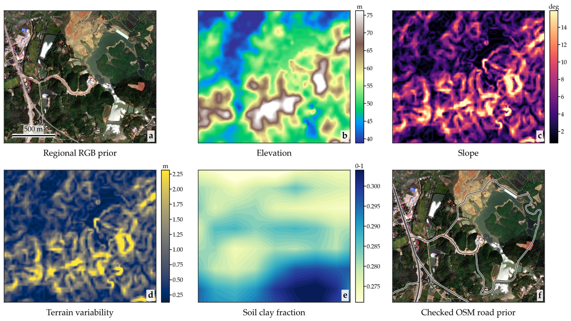
OpenEarthMap labels were harmonized into seven intermediate land-cover classes, then mapped to the task-oriented $C_0$–$C_4$ scheme. The source data were divided geographically into 2388 training, 539 validation, and 573 test images. SegFormer-B2 with a MiT-B2 encoder and DeepLabV3+-ResNet50 were initialized with ImageNet-pretrained weights and trained for up to 50 epochs using AdamW, a batch size of 8, an initial learning rate of 1 × 10⁻⁴, a minimum learning rate of 1 × 10⁻⁶, and a weight decay of 5 × 10⁻⁴. For target-area inference, RGB values were scaled to [0, 1] and normalized using the ImageNet mean and standard deviation. The regional image was processed using 512 × 512-pixel windows with a 128-pixel overlap, and Hanning-window blending was applied to reduce tile-edge artifacts. OSM, terrain, and soil variables were not used by the standalone image classifier. The multi-source inputs used for regional prior-map construction are summarized in Figure 3.

Target-domain performance was evaluated using a manually co-registered $C_0$–$C_4$ reference raster containing 1,797,428 valid pixels at 0.5525 m spacing. The labels occupied 25 connected, spatially separated review regions. Model-assisted pre-annotations were completely checked and corrected by a human interpreter. No target-domain reference label was used for source-domain training or checkpoint selection. Predictions were bilinearly aligned to the unchanged reference grid and renormalized before argmax classification; the reference raster, itself, was not resampled. Confidence intervals were obtained from 2000 bootstrap samples using the spatial review region, rather than individual pixels, as the resampling unit.

As shown in

Table 4. Standalone target-domain $C_0$–$C_4$ semantic performance.

Method	OA (%)	mIoU (%)	Macro-F1 (%)	Kappa	OA 95% CI (%)	mIoU 95% CI (%)
DeepLabV3+-ResNet50	80.42	57.48	72.14	0.704	74.39–85.74	46.73–64.42
SegFormer-B2	85.21	65.36	78.20	0.778	80.24–89.42	56.60–72.70

, SegFormer-B2 achieved 85.21% OA, 65.36% mIoU, 78.20% Macro-F1, and a kappa value of 0.778. DeepLabV3+-ResNet50 achieved 80.42% OA, 57.48% mIoU, 72.14% Macro-F1, and a kappa value of 0.704. The corresponding 95% confidence intervals are also reported in Table 4.

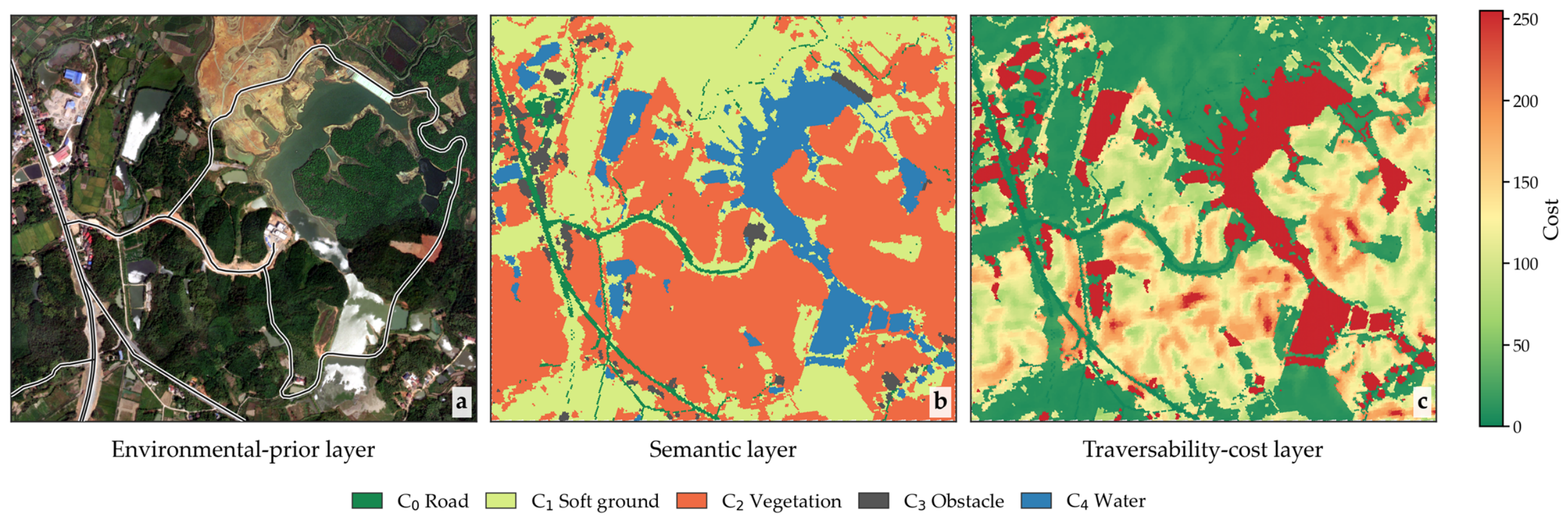
Figure 4 shows the environmental-prior, semantic, and traversability-cost layers of the off-road traversability map. Figure 5 presents representative target-domain predictions and the corresponding confusion matrix.

4.2.2. Grid-Level Fusion Benchmark

The grid-level reference was created by aggregating manually reviewed regional labels to H3-12 cells. Cells were retained when reference coverage was at least 70% and dominant-class purity was at least 60%. The benchmark contained 1713 cells: 496 cells from seven connected spatial regions were used exclusively for parameter calibration, and 1217 cells from 15 disjoint regions formed the frozen test set. Mixed cells were retained when they met the purity criterion, and their class fractions were preserved in the reference record.

All

Table 5. Grid-level comparison of CHCRM and fusion baselines on the frozen H3-12 test set. The best results are highlighted in bold, and the second-best results are underlined.

Method	OA (%)	Macro-F1 (%)	mIoU (%)	High-Risk Precision (%)	High-Risk Recall (%)	Dangerous FN
Regional semantic baseline	90.55	85.12	76.16	96.55	85.22	34
Weighted voting	90.55	84.97	76.03	96.55	85.22	34
Dempster–Shafer fusion	90.63	85.02	76.10	96.55	85.22	34
Random forest	90.47	84.68	75.82	95.73	87.83	28
CHCRM	90.96	85.49	76.77	95.75	88.26	27

predictions are paired on the same 1217 H3 cells. Relative to the regional semantic baseline, CHCRM corrected seven five-class decisions and degraded two; the two-sided exact McNemar test was not significant (p = 0.1797). Thus, the OA change from 90.55% to 90.96% is not interpreted as statistically significant. Within the 230 reference high-risk cells, CHCRM recovered seven baseline misses without losing a baseline true positive (two-sided exact paired p = 0.0156), reducing dangerous false negatives from 34 to 27. Relative to Random Forest, the one-cell reduction from 28 to 27 false negatives was not significant. The regional baseline, weighted voting, and Dempster–Shafer variants have identical high-risk statistics because their thresholded $C_3$/$C_4$ masks are identical on all evaluated cells, although non-high-risk assignments may differ.

4.2.3. Planning-Level Cost Sensitivity

Thirty paired start-goal cases were evaluated. Each ablation generated its own route, and every route was evaluated on the common full-cost surface.

Table 6. Planning-level sensitivity of the traversability-cost modifiers across 30 paired start-goal cases.

Ablation Relative to Full Model	Mean Δ Path Length, m (95% CI)	Mean Δ Common Cost/m (95% CI)	Mean Δ Soil-Risk Exposure (95% CI)	Mean Δ High-Relief Fraction (95% CI)
No slope modifier	0.00 [0.00, 0.00]	0.000 [0.000, 0.000]	0.0000 [0.0000, 0.0000]	0.0000 [0.0000, 0.0000]
No soil-wetness modifier	+12.50 [−59.10, 124.76]	−0.103 [−0.700, 0.249]	+0.0077 [0.0018, 0.0119]	−0.0006 [−0.0019, 0.0003]
No regional-relief modifier	−0.12 [−4.82, 4.96]	+0.306 [0.181, 0.467]	−0.0077 [−0.0100, −0.0059]	+0.0003 [−0.0016, 0.0018]

reports the mean within-case difference between each ablation and the full model, together with a 95% case-bootstrap confidence interval.

The paired analysis does not support a general claim that every modifier changes route geometry. Removing slope reproduced the full-model route in all 30 cases. Removing soil wetness changed mean soil-risk exposure by +0.0077 (95% CI, 0.0018 to 0.0119), while its route-length interval included zero. Removing regional relief increased common full-model cost per meter by 0.306 (95% CI, 0.181 to 0.467), while its route-length difference was centered near zero. Soil and relief terms therefore altered exposure or common-cost quality without producing a clear mean change in route length; the slope term showed no observable effect in this sample.

4.3. UAV Semantic Observation

4.3.1. Unified Buffered Spatial Benchmark

Table 7. Unified UAV semantic-observer comparison on the fixed buffered spatial test set (mean ± SD over seeds 42–44). The best results are highlighted in bold, and the second-best results are underlined.

Model	Input	OA (%)	mIoU (%)	C0 IoU	C1 IoU	C2 IoU	C3 IoU	C4 IoU
DeepLabV3+-ResNet50	RGB	83.68 ± 0.13	60.77 ± 0.76	42.20	60.74	83.03	20.60	97.29
UNetFormer-ResNet18	RGB	83.91 ± 0.19	62.91 ± 0.71	47.75	58.04	83.57	29.36	95.84
SegFormer-B2	RGB	88.06 ± 0.28	70.22 ± 0.59	56.48	66.94	87.17	41.88	98.62
CMX-B2	RGB–DSM	86.74 ± 0.12	67.76 ± 0.56	50.02	64.17	86.59	39.71	98.32
SegFormer-B2 early fusion	RGB–DSM	86.73 ± 0.08	66.37 ± 0.13	47.66	65.51	86.67	33.69	98.31
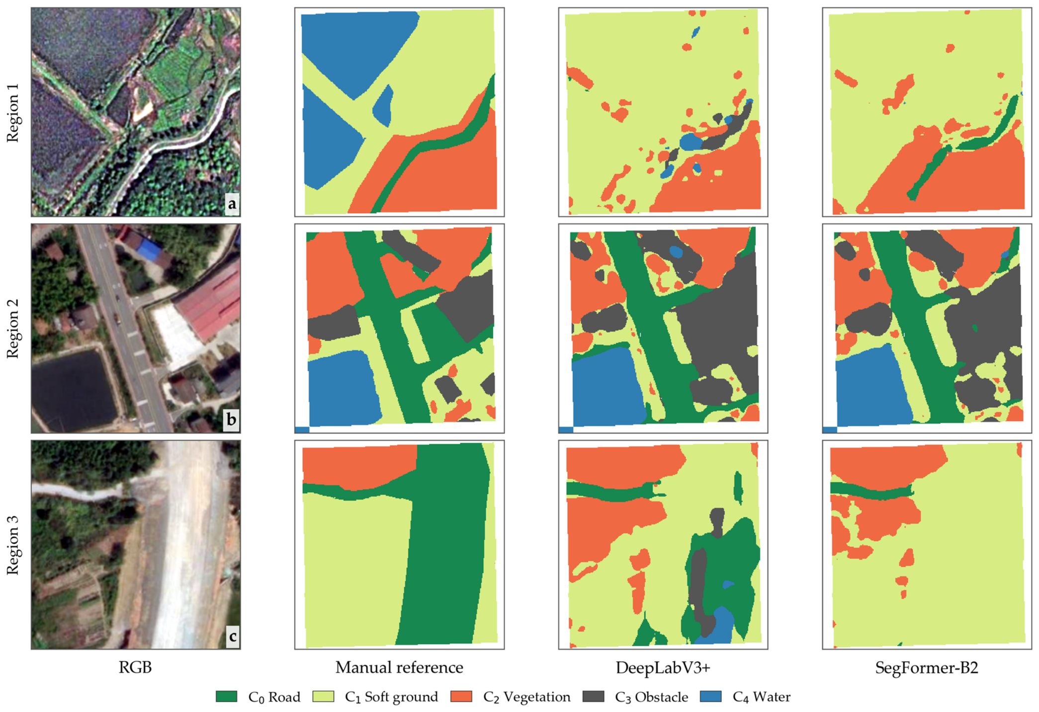
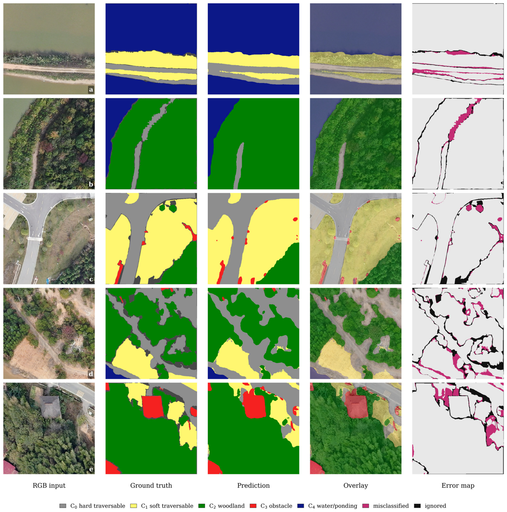
Task-adapted MFNet	RGB–DSM	83.18 ± 0.17	62.22 ± 0.63	40.52	57.97	82.60	32.86	97.15

provides the sole basis for cross-model spatial-generalization comparisons. SegFormer-B2 achieved the highest mIoU (70.22 ± 0.59%) and OA (88.06 ± 0.28%) and the highest IoU for every evaluated class. CMX-B2 was the strongest RGB–DSM model at 67.76 ± 0.56% mIoU, followed by early-fusion SegFormer-B2, at 66.37 ± 0.13%. UNetFormer-ResNet18 achieved 62.91 ± 0.71%, Task-adapted MFNet achieved 62.22 ± 0.63%, and DeepLabV3+-ResNet50 achieved 60.77 ± 0.76%. Relative to RGB-only SegFormer-B2, the paired mean mIoU differences were −2.45 percentage points for CMX-B2 (95% spatial-block bootstrap interval, −4.58 to −1.26), −3.84 points for early fusion (−7.39 to −0.65), and −8.00 points for Task-adapted MFNet (−13.85 to −5.09). Because the independent test set contains eight spatial blocks, these intervals are treated as descriptive uncertainty rather than definitive population-level inference. Under the evaluated data and protocol, DSM therefore provided no observed spatial-generalization gain. SegFormer-B2 was selected as the principal UAV observer, while Task-adapted MFNet was propagated downstream only as a secondary comparator with a distinct precision–recall profile. Representative UAV semantic observations on spatially held-out test tiles are shown in Figure 6.

4.3.2. Model Complexity and Inference Efficiency

Computational complexity was measured for 512 × 512 inputs on an NVIDIA GeForce RTX 3090. Throughput was measured with batch size of one over 50 timed forward passes following 10 warm-up passes.

Table 8. Complexity and inference throughput of the principal UAV semantic observers. The best results are highlighted in bold, and the second-best results are underlined.

Observer	Input	Parameters (M)	GFLOPs	FPS
DeepLabV3+-ResNet50	RGB	26.68	36.93	137.52
UNetFormer-ResNet18	RGB	11.72	11.74	247.74
SegFormer-B2	RGB	24.72	21.21	84.62
CMX-B2	RGB–DSM	66.56	57.03	33.08
SegFormer-B2 early fusion	RGB–DSM	24.73	21.26	90.62
Task-adapted MFNet	RGB–DSM	98.06	74.18	17.56

reports the total parameters, GFLOPs, and mean single-tile throughput for all six observers. These hardware- and implementation-dependent values support relative comparison only.

SegFormer-B2 required 24.72 M parameters and 21.21 GFLOPs and achieved 84.62 FPS. UNetFormer-ResNet18 was the lightest and fastest observer, requiring 11.72 M parameters and 11.74 GFLOPs and achieving 247.74 FPS, but its mIoU was 7.30 percentage points below that of SegFormer-B2. DeepLabV3+-ResNet50 required 26.68 M parameters and 36.93 GFLOPs and achieved 137.52 FPS. Task-adapted MFNet required 98.06 M parameters and 74.18 GFLOPs and achieved 17.56 FPS, while CMX-B2 achieved 33.08 FPS and early-fusion SegFormer-B2 achieved 90.62 FPS. Table 7 and Table 8 therefore support SegFormer-B2 as the accuracy-oriented principal observer with moderate computational complexity rather than as the absolute fastest model.

4.4. Incremental Updating, Spatial Accuracy, and Replanning

Downstream updating used the 41 images in the independent test partition of the fixed buffered spatial split. No test image contributed to optimization, early stopping, hyperparameter selection, or checkpoint selection. The frozen seed-42 SegFormer-B2 and Task-adapted MFNet checkpoints produced observations for 3398 H3-13 cells. Among them, 2391 cells overlapped the regional-prior support and formed the common evaluation domain for

Table 9. High-risk accuracy of the regional prior and three UAV update strategies on 2391 common-support H3-13 cells. The best results are highlighted in bold, and the second-best results are underlined.

Observer	Update Strategy	TP	FP	FN	TN	Precision (%)	Recall (%)	F1 (%)	OA (%)
Regional prior	Prior	518	57	64	1752	90.09	89.00	89.54	94.94
SegFormer-B2	UAV only	559	12	23	1797	97.90	96.05	96.96	98.54
SegFormer-B2	Conservative union	560	68	22	1741	89.17	96.22	92.56	96.24
SegFormer-B2	UAV override	559	12	23	1797	97.90	96.05	96.96	98.54
Task-adapted MFNet	UAV only	566	69	16	1740	89.13	97.25	93.02	96.45
Task-adapted MFNet	Conservative union	566	122	16	1687	82.27	97.25	89.13	94.23
Task-adapted MFNet	UAV override	566	69	16	1740	89.13	97.25	93.02	96.45

and the replanning experiment. The remaining 1007 cells were excluded from fusion and planning comparisons because they lacked regional-prior support.

$$\mathrm{P}\mathrm{r}\mathrm{e}\mathrm{c}\mathrm{i}\mathrm{s}\mathrm{i}\mathrm{o}\mathrm{n}={\displaystyle \frac{TP}{TP+FP}}, \mathrm{R}\mathrm{e}\mathrm{c}\mathrm{a}\mathrm{l}\mathrm{l}={\displaystyle \frac{TP}{TP+FN}}$$

(21)

where $TP$ is the number of reference high-risk cells correctly identified as high risk, $FP$ is the number of reference non-high-risk cells incorrectly identified as high risk, and $FN$ is the number of reference high-risk cells missed by the evaluated map state. Precision measures alarm reliability, while recall measures high-risk coverage. $F_1$ and overall accuracy were calculated using Equation (22).

$$F_1={\displaystyle \frac{2\hspace{0.17em}\mathrm{P}\mathrm{r}\mathrm{e}\mathrm{c}\mathrm{i}\mathrm{s}\mathrm{i}\mathrm{o}\mathrm{n}\hspace{0.17em}\mathrm{R}\mathrm{e}\mathrm{c}\mathrm{a}\mathrm{l}\mathrm{l}}{\mathrm{P}\mathrm{r}\mathrm{e}\mathrm{c}\mathrm{i}\mathrm{s}\mathrm{i}\mathrm{o}\mathrm{n}+\mathrm{R}\mathrm{e}\mathrm{c}\mathrm{a}\mathrm{l}\mathrm{l}}}, OA={\displaystyle \frac{TP+TN}{TP+FP+FN+TN}}$$

(22)

where $F_1$ is the harmonic mean of high-risk precision and recall, $OA$ is binary high-risk/non-high-risk accuracy, and $FN$ is the number of correctly identified non-high-risk cells. All four counts are computed on the same 2391 common-support H3-13 cells.

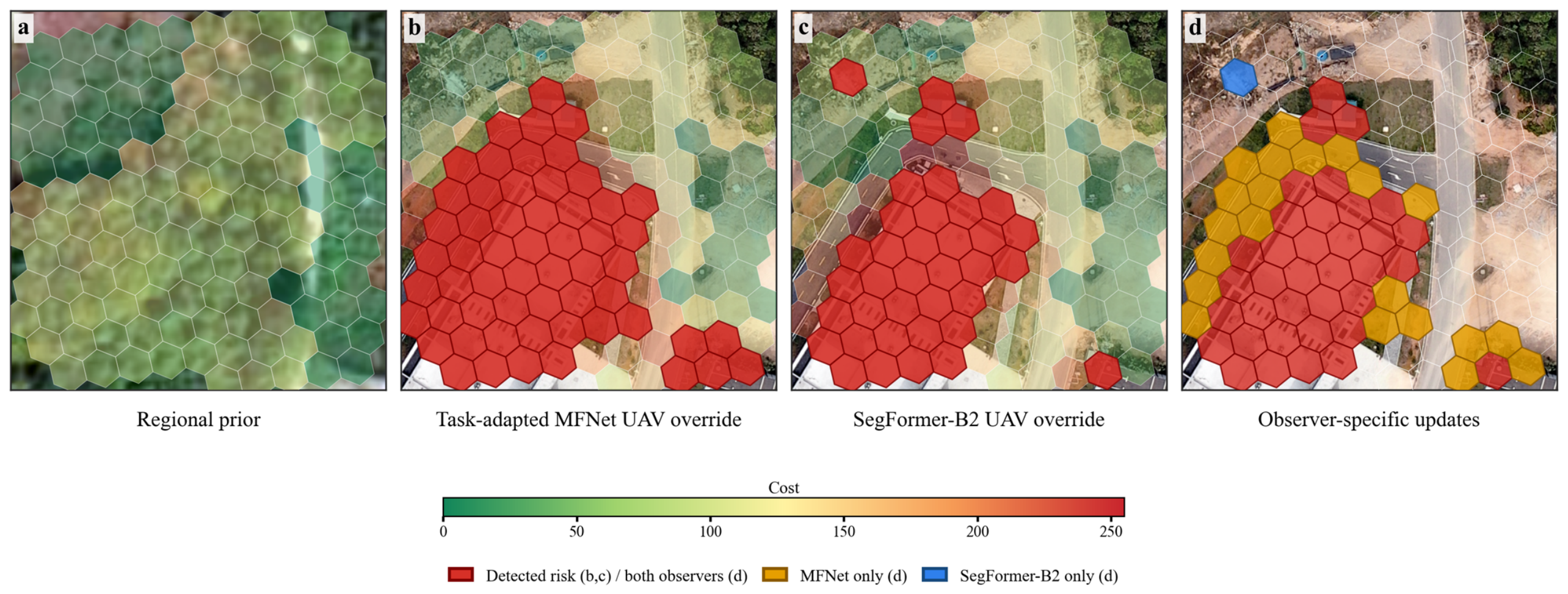
Table 9 separates observer quality from update strategy on the same 2391-cell domain. SegFormer-B2 override achieved 97.90% precision, 96.05% recall, and 96.96% F1, whereas Task-adapted MFNet override achieved 89.13% precision, 97.25% recall, and 93.02% F1. Relative to override, conservative union added one true positive and 56 false positives for SegFormer-B2. For Task-adapted MFNet, union added no true positive and 53 false positives. UAV override is therefore the principal update rule, while conservative union is retained as a safety-biased sensitivity condition. Figure 7 illustrates the pre-update prior, the two observer-specific updates, and their local agreement pattern. The figure is qualitative and does not contribute to the estimates in Table 9.

The replanning experiment used the same 40 start-goal tasks for every observer and update strategy. Each task was constructed from a manually confirmed true-new-risk cell, and its prior route crossed at least one such cell. Case selection did not use either observer’s predictions. Cells assigned a traversability cost of 255 were treated as impassable. If excluding these cells disconnected the planning graph, the case was recorded as having no feasible route. A feasible route was reference-safe when it intersected no manually confirmed high-risk cell.

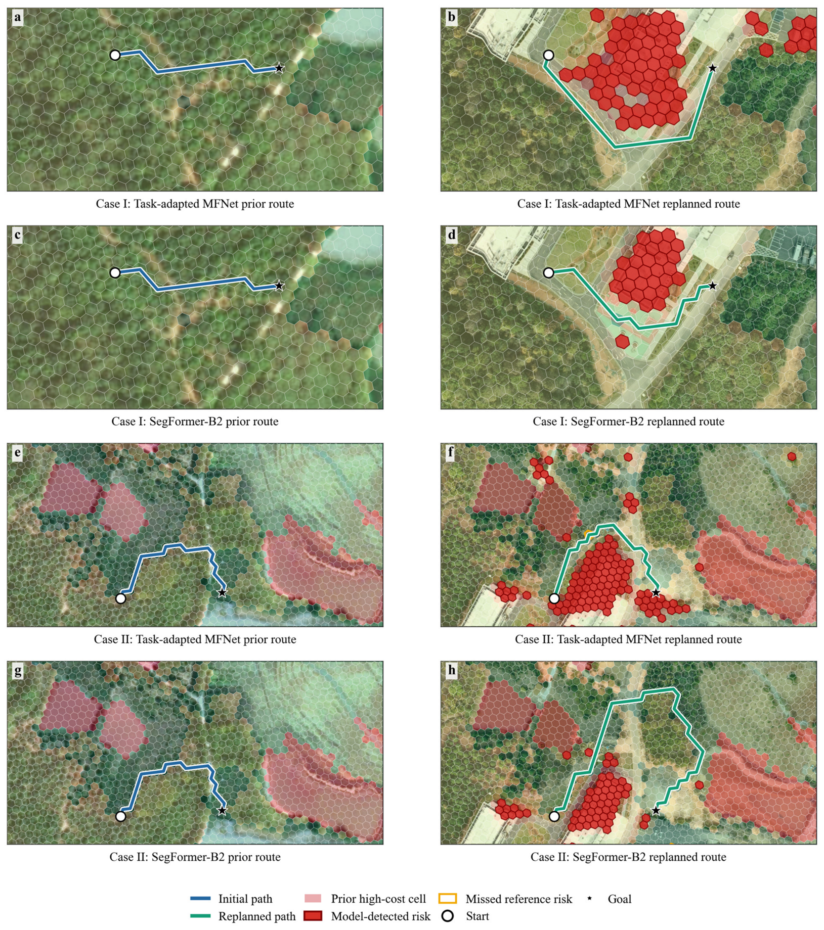
Under hard blocking, SegFormer-B2 detected 26 of 40 target risks and retained 33 feasible routes, whereas Task-adapted MFNet detected 32 targets and retained 31 feasible routes. Among feasible routes, the mean reference-risk reduction was 1.67 cells for SegFormer-B2 (95% bootstrap CI, 1.21–2.15; Wilcoxon p = 2.88 × 10⁻⁶) and 2.06 cells for Task-adapted MFNet (1.68–2.48; p = 1.07 × 10⁻⁶). Conservative union and UAV override produced identical feasibility and paths in all 40 tasks for both observers. The no-route outcomes therefore arose from newly detected hard blocks rather than from retained prior-only risks. A finite cost of 200 restored all 40 routes for both observers, but reference-safe rates decreased to 37.5% for SegFormer-B2 and 55.0% for Task-adapted MFNet. Figure 8 provides qualitative route examples in two preselected regions;

Table 10. Fixed 40-case replanning comparison for two frozen observers, two hard-update strategies, and a finite soft-cost sensitivity condition.

Observer	Planner Update	Feasible Routes	No Route	Target Detected (%)	Reference-Safe Among Feasible (%)	Risk Hits Before → After
SegFormer-B2	Conservative union, hard 255	33/40	7	65.0	54.5	2.27 → 0.61
SegFormer-B2	UAV override, hard 255	33/40	7	65.0	54.5	2.27 → 0.61
SegFormer-B2	Soft penalty 200	40/40	0	65.0	37.5	2.80 → 0.95
Task-adapted MFNet	Conservative union, hard 255	31/40	9	80.0	80.6	2.29 → 0.23
Task-adapted MFNet	UAV override, hard 255	31/40	9	80.0	80.6	2.29 → 0.23
Task-adapted MFNet	Soft penalty 200	40/40	0	80.0	55.0	2.80 → 0.68

remains the basis for quantitative comparison.

5. Discussion

The main significance of this study lies in integrating regional prior mapping, local UAV observation, incremental updating, and global replanning within a unified workflow. Regional remote-sensing products provide broad spatial coverage before deployment, whereas UAV observations provide current information for selected areas. A common H3 index connects these sources without requiring reconstruction of the entire regional map. The workflow therefore extends static remote-sensing products toward a maintainable off-road traversability map.

The layered map structure separates source evidence, semantic interpretation, and planner-ready costs. This separation preserves data provenance and allows semantic and cost states to be updated without overwriting the original regional evidence. CHCRM reduced omissions within the evaluated high-risk subset, but it did not significantly improve overall five-class accuracy. Its contribution should therefore be interpreted as targeted conflict resolution for safety-relevant terrain rather than universal improvement across all semantic classes.

The six-model benchmark further distinguishes semantic accuracy from computational efficiency and input modality. SegFormer-B2 achieved the highest semantic accuracy with moderate computational complexity. UNetFormer-ResNet18 was the lightest and fastest model, but its mIoU was 7.30 percentage points lower than that of SegFormer-B2; DeepLabV3+ also provided higher throughput but lower semantic accuracy. CMX-B2 was the strongest RGB–DSM model, yet neither it nor the same-backbone early-fusion model surpassed RGB-only SegFormer-B2. This result does not establish that DSM is intrinsically uninformative. It shows that the available DSM representation and the evaluated fusion strategies did not improve geographic generalization in this dataset. Because the benchmark combines limited spatial training support, tile-wise relative-height normalization, and DSM data without independent vertical validation, it cannot separate the effects of data quality, representation, and fusion design. DSM is therefore treated as an optional modality and not as a validated performance contribution. Downstream, Task-adapted MFNet achieved higher risk recall but generated more false positives and hard-block disconnections. Observer selection should consequently consider semantic accuracy, computational resources, missed hazards, false alarms, and route connectivity together.

The update and replanning experiments highlight the importance of explicitly defining map-management and risk policies. UAV override preserves the regional prior outside the observed footprint while allowing recent evidence to replace potentially outdated information within it. This approach is more appropriate for incremental maintenance than indiscriminately accumulating prior and current risk labels. Hard blocking and finite costs represent different operational attitudes toward risk. A disconnected route under hard blocking can indicate that additional observation or mission adjustment is required. A finite cost restores connectivity but accepts greater exposure to potentially hazardous terrain.

The workflow may support pre-mission planning in agriculture, forestry, disaster assessment, field exploration, and other large-area off-road applications. It is particularly relevant when complete high-resolution surveying is impractical, but UAV observations can be acquired for critical corridors or uncertain areas. In this context, the off-road traversability map provides global environmental guidance and may help prioritize areas requiring additional observation.

Several limitations define the scope of the present findings. The experiments cover a limited geographic and temporal setting, while SRTM and SoilGrids retain their original regional resolutions. The UAV-derived DSM was evaluated only as an optional semantic input and did not improve overall spatial generalization in the current benchmark. Its vertical accuracy was not independently validated, and tile-wise normalization does not preserve a common absolute height reference; the DSM is therefore not used to update terrain slope or relief. The study also does not evaluate closed-loop navigation with a physical ground vehicle. Future work should examine cross-region and cross-season generalization, multi-temporal change detection, uncertainty-aware updating, DSM representations with validated vertical accuracy and consistent height reference, higher-resolution terrain data, and feedback from onboard vehicle perception.

6. Conclusions

This study presents an integrated workflow for constructing and incrementally maintaining an off-road traversability map from regional remote-sensing data and local UAV observations. The workflow combines a layered map representation, H3-based spatial indexing, confidence-hierarchical conflict resolution, an observer-agnostic update interface, and risk-aware global replanning. Together, these components provide a consistent connection between heterogeneous environmental evidence and planner-ready traversability costs.

The experiments indicate that map reliability depends not only on aggregate semantic accuracy but also on observer error profiles, update policy, and the treatment of hazardous cells during planning. RGB-only SegFormer-B2 provided the highest spatially held-out semantic accuracy and was therefore selected as the primary observer. The RGB–DSM comparisons did not show a generalization gain, so DSM is retained as an optional modality rather than claimed as an effective fusion contribution. Task-adapted MFNet remains informative as a high-recall, lower-precision comparator that demonstrates how different segmentation errors propagate into map states and route feasibility. UAV override supported controlled local updating, whereas hard and finite costs exposed the trade-off between risk avoidance and connectivity.

The proposed workflow should be regarded as an upstream mapping and global-planning service. It can provide prior environmental guidance and support mission-level decisions, but it does not replace onboard localization, local obstacle avoidance, or vehicle control. Further field validation is required before the workflow can support closed-loop autonomous navigation.

References

1. Beycimen, S.; Ignatyev, D.; Zolotas, A. A comprehensive survey of unmanned ground vehicle terrain traversability for unstructured environments and sensor technology insights. Eng. Sci. Technol. Int. J. 2023, 47, 101457. [Google Scholar] [CrossRef] [Scilit]
2. Li, Y.; Tian, E.; Yang, F.; Han, H.; Zhang, X. An End-to-End Trajectory Prediction Method for Unmanned Ground Vehicles via Multimodal Fusion. Sensors 2026, 26, 4648. [Google Scholar] [CrossRef] [Scilit] [PubMed]
3. Zhou, N.; Zhang, G.; Zhu, C.; Dong, X. An unstructured roadless environment navigation map construction method based on remote sensing. Geo-Spat. Inf. Sci. 2025. [Google Scholar] [CrossRef] [Scilit]
4. Elghazaly, G.; Frank, R.; Harvey, S.; Safko, S. High-definition maps: Comprehensive survey, challenges, and future perspectives. IEEE Open J. Intell. Transp. Syst. 2023, 4, 527–550. [Google Scholar] [CrossRef] [Scilit]
5. Benrabah, M.; Orou Mousse, C.; Randriamiarintsoa, E.; Chapuis, R.; Aufrère, R. A review on traversability risk assessments for autonomous ground vehicles: Methods and metrics. Sensors 2024, 24, 1909. [Google Scholar] [CrossRef] [Scilit] [PubMed]
6. Potić, I.; Đorđević, D. Terrain passability modeling for cross-country unmanned ground vehicle navigation. Trans. GIS 2025, 29, e70035. [Google Scholar] [CrossRef] [Scilit]
7. Elfes, A. Using occupancy grids for mobile robot perception and navigation. Computer 1989, 22, 46–57. [Google Scholar] [CrossRef] [Scilit]
8. Fankhauser, P.; Hutter, M. A universal grid map library: Implementation and use case for rough terrain navigation. In Robot Operating System (ROS): The Complete Reference; Koubaa, A., Ed.; Springer: Cham, Switzerland, 2016; Volume 625, pp. 99–120. [Google Scholar] [CrossRef] [Scilit]
9. Brown, C.F.; Brumby, S.P.; Guzder-Williams, B.; Birch, T.; Hyde, S.B.; Mazzariello, J.; Czerwinski, W.; Pasquarella, V.J.; Haertel, R.; Ilyushchenko, S.; et al. Dynamic World, Near real-time global 10 m land use land cover mapping. Sci. Data 2022, 9, 251. [Google Scholar] [CrossRef] [Scilit]
10. Hawker, L.; Uhe, P.; Paulo, L.; Sosa, J.; Savage, J.; Sampson, C.; Neal, J. A 30 m global map of elevation with forests and buildings removed. Environ. Res. Lett. 2022, 17, 024016. [Google Scholar] [CrossRef] [Scilit]
11. Wang, R.; Wan, S.; Chen, W.; Qin, X.; Zhang, G.; Wang, L. A novel finer soil strength mapping framework based on machine learning and remote sensing images. Comput. Geosci. 2024, 182, 105479. [Google Scholar] [CrossRef] [Scilit]
12. Lu, X.; Weng, Q. Deep learning-based road extraction from remote sensing imagery: Progress, problems, and perspectives. ISPRS J. Photogramm. Remote Sens. 2025, 228, 122–140. [Google Scholar] [CrossRef] [Scilit]
13. Li, J.; Qin, H.; Wang, J.; Li, J. OpenStreetMap-based autonomous navigation for the four wheel-legged robot via 3D-LiDAR and CCD camera. IEEE Trans. Ind. Electron. 2022, 69, 2708–2717. [Google Scholar] [CrossRef] [Scilit]
14. Samadzadegan, F.; Toosi, A.; Dadrass Javan, F. A critical review on multi-sensor and multi-platform remote sensing data fusion approaches: Current status and prospects. Int. J. Remote Sens. 2025, 46, 1327–1402. [Google Scholar] [CrossRef] [Scilit]
15. Reyes-Rubiano, L.; Voegl, J.; Rest, K.-D.; Faulin, J.; Hirsch, P. Exploration of a disrupted road network after a disaster with an online routing algorithm. OR Spectr. 2021, 43, 289–326. [Google Scholar] [CrossRef] [Scilit]
16. Lei, T.; Zhang, S.; Lin, S.; Liu, T.; Lv, Z.; Gao, T.; Gong, M.; Nandi, A.K. Remote sensing image change detection using deep learning techniques: A comprehensive survey. Artif. Intell. Rev. 2026, 59, 102. [Google Scholar] [CrossRef] [Scilit]
17. Cheng, J.; Deng, C.; Su, Y.; An, Z.; Wang, Q. Methods and datasets on semantic segmentation for Unmanned Aerial Vehicle remote sensing images: A review. ISPRS J. Photogramm. Remote Sens. 2024, 211, 1–34. [Google Scholar] [CrossRef] [Scilit]
18. Niu, Z.; Xia, H.; Tao, P.; Ke, T. Accuracy assessment of UAV photogrammetry system with RTK measurements for direct georeferencing. ISPRS Ann. Photogramm. Remote Sens. Spat. Inf. Sci. 2024, 10, 169–176. [Google Scholar] [CrossRef] [Scilit]
19. Elias, M.; Isfort, S.; Eltner, A.; Maas, H.-G. UAS photogrammetry for precise digital elevation models of complex topography: A strategy guide. ISPRS Ann. Photogramm. Remote Sens. Spat. Inf. Sci. 2024, 10, 57–64. [Google Scholar] [CrossRef] [Scilit]
20. Ma, X.; Zhang, X.; Pun, M.-O.; Huang, B. A unified framework with multimodal fine-tuning for remote sensing semantic segmentation. IEEE Trans. Geosci. Remote Sens. 2025, 63, 5405015. [Google Scholar] [CrossRef] [Scilit]
21. Tong, Y.; Tang, M.; Zhang, Y.; Huang, Y.; Huang, J.; He, Y.; Liu, Y.; Akpokodje, E.; Zheng, D. BATFNet: Boundary-aware Transformer fusion network for RGB-DSM semantic segmentation of remote sensing images. Sensors 2026, 26, 3205. [Google Scholar] [CrossRef] [Scilit] [PubMed]
22. Luo, Z.; Gao, L.; Xiang, H.; Li, J. Road object detection for HD map: Full-element survey, analysis and perspectives. ISPRS J. Photogramm. Remote Sens. 2023, 197, 122–144. [Google Scholar] [CrossRef] [Scilit]
23. Berlenko, T.; Krinkin, K. Sensor-model matching for controlled comparison of Bayesian and belief-function occupancy grid fusion. Sensors 2026, 26, 4266. [Google Scholar] [CrossRef] [Scilit] [PubMed]
24. Erni, G.; Frey, J.; Miki, T.; Mattamala, M.; Hutter, M. MEM: Multi-modal elevation mapping for robotics and learning. In Proceedings of the 2023 IEEE/RSJ International Conference on Intelligent Robots and Systems (IROS), Detroit, MI, USA, 1–5 October 2023; pp. 11011–11018. [Google Scholar] [CrossRef] [Scilit]
25. Shu, Y.; Dong, L.; Liu, J.; Liu, C.; Wei, W. Overview of terrain traversability evaluation for autonomous robots. J. Field Robot. 2025, 42, 1724–1765. [Google Scholar] [CrossRef] [Scilit]
26. Liu, Q.; You, X.; Zhang, X.; Zuo, J. Construction of dynamic trafficability map for unmanned vehicles considering multiple environmental factors and path planning. Sci. Rep. 2025, 15, 9957. [Google Scholar] [CrossRef] [Scilit] [PubMed]
27. Zhu, C.; Zhang, G.; Zhou, N.; Qin, X.; Zou, W.; Han, Z.; Xu, Q.; Dong, X. Remote sensing-based inversion method for vehicle trafficability in off-road environments. Geomat. Inf. Sci. Wuhan Univ. 2025, 50, 2247–2259. [Google Scholar] [CrossRef]
28. Eder, M.; Prinz, R.; Schöggl, F.; Steinbauer-Wagner, G. Traversability analysis for off-road environments using locomotion experiments and earth observation data. Robot. Auton. Syst. 2023, 168, 104494. [Google Scholar] [CrossRef] [Scilit]
29. Zhang, B.; Chen, W.; Xu, C.; Qiu, J.; Chen, S. Autonomous vehicles traversability mapping fusing semantic-geometric in off-road navigation. Drones 2024, 8, 496. [Google Scholar] [CrossRef] [Scilit]
30. Jeon, Y.; Son, E.I.; Seo, S.-W. Follow the footprints: Self-supervised traversability estimation for off-road vehicle navigation based on geometric and visual cues. In Proceedings of the 2024 IEEE International Conference on Robotics and Automation (ICRA), Yokohama, Japan, 13–17 May 2024; pp. 1774–1780. [Google Scholar] [CrossRef] [Scilit]
31. Mattamala, M.; Frey, J.; Libera, P.; Chebrolu, N.; Martius, G.; Cadena, C.; Hutter, M.; Fallon, M. Wild visual navigation: Fast traversability learning via pre-trained models and online self-supervision. Auton. Robot. 2025, 49, 19. [Google Scholar] [CrossRef] [Scilit]
32. Triest, S.; Sivaprakasam, M.; Aich, S.; Fan, D.; Wang, W.; Scherer, S. Velociraptor: Leveraging visual foundation models for label-free, risk-aware off-road navigation. Proc. Mach. Learn. Res. 2025, 270, 4483–4494. [Google Scholar]
33. He, K.; Dong, Y.; Zhang, Z.; Ma, H.; Fan, R.; Wang, L. Off-road trafficability assessment with remote sensing imagery and incomplete auxiliary data via a cross-modal channel feature fusion network. IEEE Trans. Geosci. Remote Sens. 2025, 63, 4510216. [Google Scholar] [CrossRef] [Scilit]
34. Marsh, C.B.; Harder, P.; Pomeroy, J.W. Validation of FABDEM, a global bare-earth elevation model, against UAV-lidar derived elevation in a complex forested mountain catchment. Environ. Res. Commun. 2023, 5, 031009. [Google Scholar] [CrossRef] [Scilit]
35. Rengarajan, R.; Choate, M.J.; Hasan, M.N.; Denevan, A. Co-registration accuracy between Landsat-8 and Sentinel-2 orthorectified products. Remote Sens. Environ. 2024, 301, 113947. [Google Scholar] [CrossRef] [Scilit]
36. Li, J.; Hong, D.; Gao, L.; Yao, J.; Zheng, K.; Zhang, B.; Chanussot, J. Deep learning in multimodal remote sensing data fusion: A comprehensive review. Int. J. Appl. Earth Obs. Geoinf. 2022, 112, 102926. [Google Scholar] [CrossRef] [Scilit]
37. Liu, Z.; Guo, S.; Yu, F.; Hao, J.; Zhang, P. Improved A* algorithm for mobile robots under rough terrain based on ground trafficability model and ground ruggedness model. Sensors 2024, 24, 4884. [Google Scholar] [CrossRef] [Scilit] [PubMed]
38. Sahr, K.; White, D.; Kimerling, A.J. Geodesic discrete global grid systems. Cartogr. Geogr. Inf. Sci. 2003, 30, 121–134. [Google Scholar] [CrossRef] [Scilit]
39. Kmoch, A.; Matsibora, O.; Vasilyev, I.; Uuemaa, E. Applied open-source Discrete Global Grid Systems. Agil. GISci. Ser. 2022, 3, 41. [Google Scholar] [CrossRef] [Scilit]
40. Huang, X.; Ding, J.; Ben, J.; Zhou, J.; Liang, Q.; Dai, J. Advancing digital earth modeling: Hexagonal multi-structural elements in icosahedral DGGS for enhanced geospatial data processing. Environ. Model. Softw. 2024, 172, 105922. [Google Scholar] [CrossRef] [Scilit]
41. Brodsky, I. H3: Uber’s Hexagonal Hierarchical Spatial Index. Uber Engineering Blog. 2018. Available online: https://www.uber.com/blog/h3/ (accessed on 22 August 2026).
42. Nex, F.; Armenakis, C.; Cramer, M.; Cucci, D.A.; Gerke, M.; Honkavaara, E.; Kukko, A.; Persello, C.; Skaloud, J. UAV in the advent of the twenties: Where we stand and what is next. ISPRS J. Photogramm. Remote Sens. 2022, 184, 215–242. [Google Scholar] [CrossRef] [Scilit]
43. Zhi, Y.; Wang, Y.; Zhang, F.; Ma, M.; Mei, S. MSFFNet: Multimodal spatial-frequency fusion network for RGB-DSM remote sensing image segmentation. Remote Sens. 2025, 17, 3745. [Google Scholar] [CrossRef] [Scilit]
44. Ronneberger, O.; Fischer, P.; Brox, T. U-Net: Convolutional networks for biomedical image segmentation. In Medical Image Computing and Computer-Assisted Intervention (MICCAI); Springer: Cham, Switzerland, 2015; pp. 234–241. [Google Scholar] [CrossRef] [Scilit]
45. Chen, L.-C.; Zhu, Y.; Papandreou, G.; Schroff, F.; Adam, H. Encoder-decoder with atrous separable convolution for semantic image segmentation. In Proceedings of the European Conference on Computer Vision (ECCV), Munich, Germany, 8–14 September 2018; pp. 833–851. [Google Scholar] [CrossRef] [Scilit]
46. Xie, E.; Wang, W.; Yu, Z.; Anandkumar, A.; Alvarez, J.M.; Luo, P. SegFormer: Simple and efficient design for semantic segmentation with Transformers. Adv. Neural Inf. Process. Syst. 2021, 34, 12077–12090. [Google Scholar]
47. Kirillov, A.; Mintun, E.; Ravi, N.; Mao, H.; Rolland, C.; Gustafson, L.; Xiao, T.; Whitehead, S.; Berg, A.C.; Lo, W.-Y.; et al. Segment Anything. In Proceedings of the 2023 IEEE/CVF International Conference on Computer Vision (ICCV), Paris, France, 2–6 October 2023; pp. 3992–4003. [Google Scholar] [CrossRef] [Scilit]
48. Ma, X.; Wu, Q.; Zhao, X.; Zhang, X.; Pun, M.-O.; Huang, B. SAM-assisted remote sensing imagery semantic segmentation with object and boundary constraints. IEEE Trans. Geosci. Remote Sens. 2024, 62, 1–16. [Google Scholar] [CrossRef] [Scilit]
49. Hu, E.J.; Shen, Y.; Wallis, P.; Allen-Zhu, Z.; Li, Y.; Wang, S.; Wang, L.; Chen, W. LoRA: Low-rank adaptation of large language models. In Proceedings of the International Conference on Learning Representations (ICLR), Virtual Event, 25–29 April 2022; Available online: https://arxiv.org/abs/2106.09685 (accessed on 22 August 2026).
50. Lin, T.-Y.; Goyal, P.; Girshick, R.; He, K.; Dollár, P. Focal loss for dense object detection. In Proceedings of the 2017 IEEE International Conference on Computer Vision (ICCV), Venice, Italy, 22–29 October 2017; pp. 2999–3007. [Google Scholar] [CrossRef] [Scilit]
51. Berman, M.; Triki, A.R.; Blaschko, M.B. The Lovasz-Softmax loss: A tractable surrogate for the optimization of the intersection-over-union measure in neural networks. In Proceedings of the 2018 IEEE/CVF Conference on Computer Vision and Pattern Recognition (CVPR), Salt Lake City, UT, USA, 18–23 June 2018; pp. 4413–4421. [Google Scholar] [CrossRef] [Scilit]
52. Peng, D.; Liu, X.; Zhang, Y.; Guan, H.; Li, Y.; Bruzzone, L. Deep learning change detection techniques for optical remote sensing imagery: Status, perspectives and challenges. Int. J. Appl. Earth Obs. Geoinf. 2025, 136, 104282. [Google Scholar] [CrossRef] [Scilit]
53. Wang, L.; Li, R.; Zhang, C.; Fang, S.; Duan, C.; Meng, X.; Atkinson, P.M. UNetFormer: A UNet-like transformer for efficient semantic segmentation of remote sensing urban scene imagery. ISPRS J. Photogramm. Remote Sens. 2022, 190, 196–214. [Google Scholar] [CrossRef] [Scilit]
54. Zhang, J.; Liu, H.; Yang, K.; Hu, X.; Liu, R.; Stiefelhagen, R. CMX: Cross-modal fusion for RGB-X semantic segmentation with Transformers. IEEE Trans. Intell. Transp. Syst. 2023, 24, 14679–14694. [Google Scholar] [CrossRef] [Scilit]
Figure 1. Framework for regional prior-map construction and local semantic and traversability-cost updating using satellite and UAV observations.
Remotesensing 18 03045 g001
Figure 2. Representative annotated samples from the Chibi-Wild-500 dataset. Each row presents the UAV RGB image, co-registered photogrammetric DSM, and manual C 0 C 4 annotation. (a) A mixed scene containing ponds, a narrow road, woodland, and buildings; (b) an earthwork scene containing unpaved roads, exposed ground, vegetation, and buildings; (c) a road-junction scene surrounded by woodland, buildings, and a small water body; (d) a reservoir-edge scene containing water, an embankment road, vegetation, and an engineered structure. The annotation colors represent C 0 hard traversable, C 1 soft traversable, C 2 woodland, C 3 obstacle, C 4 water/ponding, and ignored areas. The DSM panels were independently normalized for visualization. The shared colour scale therefore indicates relative elevation from low to high within each displayed sample, rather than a common absolute elevation range.
Remotesensing 18 03045 g002
Figure 3. Regional inputs used to construct the off-road traversability map. (a) Regional RGB imagery used to derive the semantic prior; (b) SRTM-derived elevation; (c) SRTM-derived slope; (d) SRTM-derived regional relief variability; (e) SoilGrids clay fraction used as regional wet-soft susceptibility evidence; (f) manually checked OSM road-corridor prior. The color bars in (be) indicate the corresponding units or normalized range.
Remotesensing 18 03045 g003
Figure 4. Three-layer structure of the constructed off-road traversability map. (a) Environmental-prior layer containing regional source evidence and the checked road prior; (b) semantic layer containing the fused C 0 C 4 traversability classes; (c) traversability-cost layer containing the planner-ready integrated costs. The color scale in (c) ranges from lower traversal cost to the non-traversable blocking value.
Remotesensing 18 03045 g004
Figure 5. Representative target-domain comparison of regional C 0 C 4 semantic predictions. Each row presents the regional RGB image, manually reviewed reference, DeepLabV3+-ResNet50 prediction, and SegFormer-B2 prediction. (a) Region 1, containing water, soft traversable ground, vegetation, and a narrow road corridor; (b) Region 2, containing a road intersection, buildings, vegetation, and an adjacent water body; (c) Region 3, containing a linear hard-traversable road bordered by soft ground and vegetation. The colors represent C 0 hard traversable, C 1 soft traversable, C 2 woodland, C 3 obstacle, and C 4 water/ponding. Model predictions are displayed within the manually reviewed spatial support. White margins denote ignored pixels that were excluded from quantitative evaluation.
Remotesensing 18 03045 g005
Figure 6. Representative UAV C 0 C 4 semantic observations. Each row presents the RGB input, manually annotated ground truth, model prediction, prediction overlay, and error map. (a) A narrow traversable corridor between water/ponding areas; (b) a woodland-dominated corridor adjacent to water; (c) a paved-road intersection surrounded by soft ground, woodland, and small obstacles; (d) a transition area containing woodland and exposed traversable surfaces; (e) a building obstacle surrounded by woodland and soft ground. The colors represent C 0 hard traversable, C 2 soft traversable, C 2 woodland, C 3 obstacle, C 4 water/ponding, misclassified pixels, and ignored pixels.
Remotesensing 18 03045 g006
Figure 7. Qualitative illustration of UAV-driven cost updating in one representative local region. (a) Pre-update regional prior cost on the Esri basemap without UAV observation overlays; (b) UAV-override cost from the previously generated Task-adapted MFNet observation; (c) UAV-override cost from the frozen SegFormer-B2 observation; (d) agreement and observer-specific new-risk detections on the UAV DOM. Red cells in (b,c) denote detected new risks. In (d), red denotes detections shared by both observers, orange denotes MFNet-only detections, and blue denotes SegFormer-B2-only detections. The horizontal cost scale applies to panels (ac). This qualitative region is separate from the quantitative evaluation domain used in Table 9.
Remotesensing 18 03045 g007
Figure 8. Qualitative replanning comparison between Task-adapted MFNet and SegFormer-B2 in two illustrative start-goal regions. (a,b) Task-adapted MFNet in Case I; (c,d) SegFormer-B2 in Case I; (e,f) Task-adapted MFNet in Case II; (g,h) SegFormer-B2 in Case II. Each before–after pair uses the same spatial extent and continuous set of valid H3 cells. Prior-route panels show only the pre-update Esri basemap and prior-cost grid. UAV-derived risk overlays appear only in the replanned-route panels. Red cells denote model-detected new risks, orange outlines denote missed reference-risk cells, and blue and green lines denote initial and replanned paths, respectively. These qualitative examples do not contribute to the fixed 40-case results in Table 10.
Remotesensing 18 03045 g008