Retrospective Forest Volume Estimation in Southern Chile Using ALOS-PALSAR for Carbon MRV Applications

Highlights

What are the main findings?

• Historical ALOS-PALSAR L-band SAR mosaics combined with Chile’s Continuous National Forest Inventory enabled retrospective estimation of forest volume and carbon stocks across approximately 42,000 km² of native forests in southern Chile.
• Despite pixel-level uncertainty and SAR signal saturation in high-volume stands, the methodology successfully reproduced broad regional patterns of forest structure and carbon distribution relevant for carbon accounting.

What is the implication of the main finding?

• Historical SAR archives provide a practical Tier-3 approach for reconstructing forest carbon baselines in remote and persistently cloudy regions where field inventories and optical remote sensing are limited.
• The methodology can support greenhouse-gas inventories, REDD+ implementation, and MRV systems by generating spatially explicit historical carbon estimates for data-limited forest regions.

Abstract

Accurate historical estimates of forest carbon stocks are essential for greenhouse gas inventories and REDD+ Measurement, Reporting and Verification (MRV) systems, particularly in remote and persistently cloudy regions where field inventories and optical remote sensing are limited. This study presents a retrospective mapping framework with potential relevance for Tier-3 forest carbon estimation of forest volume and carbon stocks in the temperate forests of southern Chile using historical ALOS PALSAR L-band SAR data integrated with Chile’s Continuous National Forest Inventory (CNFI). Three pilot zones in Los Lagos, Aysén, and Magallanes were analysed, covering approximately 42,000 km² of native forests dominated by Lenga, Coihue de Magallanes, Siempreverde, Roble–Raulí–Coihue, Coihue–Raulí–Tepa, and Alerce forest types. Annual 25 m ALOS PALSAR mosaics were processed to derive HH and HV backscatter, HH/HV ratio, and Radar Forest Degradation Index (RFDI) layers, which were used as predictors in k-nearest neighbours (k-NN) models calibrated with inventory plots projected to the 2010 reference year. Model performance varied substantially among forest types and pilot zones, with test r² values ranging from 0.12 to 0.90 and RMSE values between approximately 100 and 300 m³·ha⁻¹; the highest r² values were associated with forest types represented by relatively small samples and should therefore be interpreted cautiously. m³·ha⁻¹ Stratification by altitude and restriction to moderate volume ranges improved predictive performance in several cases, highlighting the influence of ecological gradients and SAR signal saturation at high levels of biomass. Despite substantial pixel-level uncertainty, the methodology reproduced broad regional patterns of forest structure and carbon distribution. Results demonstrate the potential of combining historical ALOS PALSAR archives with national forest inventories to support spatially explicit historical carbon estimation in data-limited forest regions.

1. Introduction

Quantifying forest carbon stocks with high accuracy is an important component of national greenhouse gas inventories and climate change mitigation strategies [1]. However, achieving accurate estimates over diverse national territories requires methodologies tailored to local environmental conditions and data availability. Global or generic forest volume or biomass maps often fail to capture the fine-scale variability at national and sub-national levels, prompting the need for country-specific Tier-3 approaches that integrate detailed ground data with advanced modeling or remote sensing [2,3]. Forest inventory data in many tropical and densely forested regions remain limited and uneven in quality, as the implementation of comprehensive field inventories is particularly challenging in extensive and often inaccessible forest landscapes, resulting in reliance on lower-tier data and default biomass models [4]. The Intergovernmental Panel on Climate Change (IPCC) defines Tier-3 methods as those employing high-resolution, country-specific data (e.g., extensive field inventories) and dynamic models to better represent local forest carbon dynamics, in contrast to regional average values [2]. Adopting such robust methods is especially important for regions with unique ecosystems and challenging monitoring conditions. Southern Chile is a prime example of the need for locally adapted advanced methodologies.

The Magallanes, Aysén, and Los Lagos regions of Chilean Patagonia host the largest temperate forest expanse in the Southern Hemisphere [5], representing 68% of Chile’s native forests [6]. These relatively pristine ecosystems are globally notable for their exceptionally high carbon densities, often exceeding those of tropical or boreal forests [7]. Dominant types include Lenga (Nothofagus pumilio), Coihue de Magallanes (N. betuloides), and Siempreverde, complemented by Roble–Raulí–Coihue, Coihue–Raulí–Tepa, and emblematic formations such as Alerce, alongside protected species like Araucaria and Ciprés de las Guaitecas [6]. At the southern tip of Chile (56°S), vast expanses of deciduous Lenga forests are interspersed with evergreen Coihue de Magallanes along the fjords, both adapting structurally to harsh conditions. Further north, landscapes become more diverse, hosting a broader array of forest types whose structures reflect legacies of past management. Precise estimation of carbon stocks in these extensive, heterogeneous forests is fundamental both for Chile’s national greenhouse gas inventories, which use 2001–2010 as a baseline period for emissions reporting [8], and for global carbon cycle assessments that inform international climate commitments. However, their remoteness and complexity pose challenges for monitoring: steep terrain, roadless areas, and dense vegetation limit field access, leading Chile’s Continuous National Forest Inventory (CNFI) to under sample the most carbon rich stands [5]. In addition, persistent cloud cover and heavy rainfall constrain optical monitoring (e.g., Landsat or Sentinel-2) and even compositing strategies often leave significant data gaps [6,7,8,9].

Integrating remote sensing technologies with National Forest Inventories (NFIs) enhances the accuracy and reliability of forest attribute estimates [10,11,12]. By combining field measurements with satellite optical or Synthetic Aperture Radar (SAR) data, it is possible to generate spatially continuous and temporally consistent inventories enabling more precise assessments of biomass, species composition, and other key variables [12,13]. Several studies have demonstrated that k-NN is particularly effective for estimating forest volume or biomass in heterogeneous forests using optical and SAR satellite data, especially in contexts where NFI data are sparse [14,15,16,17]. By leveraging available remote sensing information, k-NN can help compensate for the lack of extensive field data and thereby support more effective large-scale monitoring.

SAR is particularly effective in dense forest environments where optical imagery is limited [18,19,20,21]. Operating independently of weather and daylight conditions, SAR penetrates clouds and, at longer wavelengths, vegetation canopies [20,21]. L and P band systems are especially sensitive to forest structure and biomass [18,22,23], as they interact with trunks and branches and saturate at higher aboveground biomass levels than shorter wavelength [18,21]. This makes them indispensable for monitoring persistently cloudy regions. Recent satellite missions such as ESA’s BIOMASS (launched April 2025) and NASA-ISRO’s NISAR (launched July 2025) are poised to improve global forest biomass estimates. The BIOMASS mission employs a pioneering P-band SAR [24], enabling canopy penetration and large-scale wall-to-wall biomass mapping in dense tropical forests. Meanwhile, NISAR is designed to deliver global biomass retrieval at 1 ha resolution with expected accuracy of around 20 T ha⁻¹, offering reliable biomass estimation with frequent repeat coverage [25]. For retrospective estimations prior to the 2025 era the JAXA’s ALOS PALSAR remains the only suitable long-term archive for large-scale forest biomass estimation.

JAXA produces global ALOS PALSAR annual mosaics by assembling SAR backscatter images and applying corrections for geometric distortions and topographic effects on intensity [26]. These mosaics are generated annually (for period 2007–2010 using PALSAR-1 data) and are freely available as 25 m gamma-0 backscatter products [27]. The ALOS PALSAR L-band SAR mosaics have been widely used to estimate forest volume, biomass, and carbon pools across ecosystems ranging from tropical forests and mangroves to savannahs and mountain regions. Approaches vary from empirical regressions between backscatter and volume/biomass or carbon to advanced machine-learning methods such as Random Forest, boosted trees, and Bayesian inversion, often enhanced with texture or topographic variables. Reported accuracies differ, with signal saturation typically occurring between 85 and 200 Mg·ha⁻¹. When ancillary predictors are included, R² values above 0.8 are common. Applications span continental-scale biomass mapping [22,23], national-level biomass estimation using PALSAR mosaics and field inventory data [28], multiyear biomass and carbon mapping using combined PALSAR and Landsat-derived tree-cover data [29], regional forest and mangrove monitoring [30,31], and disturbance detection [32], directly contributing to carbon accounting and REDD+ initiatives. Reported RMSE values range from 8 to 117 Mg·ha⁻¹, depending on forest type, structural complexity, and methodological design (

Table 1. Representative studies using ALOS PALSAR mosaics for forest volume, aboveground biomass, carbon estimation, and related forest-monitoring applications.

Authors (et al.)	Region/Ecosystem	Methodology	Accuracy (r/r2/R2/RMSE)
Avtar et al. (2013) [28]	Tropical forests, Cambodia	Multiple linear regression using ALOS PALSAR 50 m mosaic (HV and HH/HV) calibrated with field inventory plots	R2 = 0.61; RMSE = 21 Mg ha−1 (validation up to 200 Mg ha−1)
Bouvet et al. (2018) [22]	African savannahs and woodlands	Direct model relating PALSAR backscatter to AGB + Bayesian inversion	r = 0.64–0.77; RMSD: 8–17 Mg·ha−1
Mermoz et al. (2014) [23]	Cameroon savannah	Regression model using in situ data and PALSAR mosaic	r = 0.89; RMSE: 38.4 Mg·ha−1. RMSE (<150 Mg·ha−1): 32.0 Mg·ha−1
Hamdan et al. (2014) [30]	Mangroves (Malaysia)	HV backscatter correlation with field plots	R2 = 0.427, RMSE: ±33.90 Mg ha−1
Thapa et al. (2015) [31]	Tropical Sumatra forests	Regression using gamma-naught backscatter and texture features	R2 = 0.84; RMSE = 28 Mg C·ha−1 (texture incl.)
Mermoz and Le Toan (2016) [32]	SE Asia (Vietnam, Cambodia, Lao)	SAR change detection + expectation maximization (fuzzy logic) for disturbance and regrowth assessment	Mean Producer’s Accuracy (PA): 84.7% Mean User’s Accuracy (UA): 96.3%
Thumaty et al. (2016) [33]	Deciduous forests (India)	Empirical model with HV backscatter	R2 = 0.509; RMSE = ±19.32 t·ha−1
Ma et al. (2017) [34]	NE China forests	GLM vs. boosted regression trees (GBM) using PALSAR + topography and stand structure	R2 up to 0.98; RMSE = 3.8–19.9 Mg·ha−1
Ho Tong Minh et al. (2018) [29]	Madagascar tropical forests	Integration of ALOS PALSAR HV backscatter with Landsat tree-cover fraction using piecewise exponential and linear regression with bias correction	Improved relationship from R2 ≈ 0.34 (HV only) to R2 ≈ 0.77 (tree-cover-weighted HV) for AGB <150 Mg ha−1.
Ningthoujam et al. (2018) [35]	Tropical deciduous (India)	Regression + MIMICS-I scattering model	R2 = 0.53–0.55; error: 92–94 Mg·ha−1
Omar and Misman (2018) [36]	Dipterocarpus (Malaysia)	Time-series PALSAR/PALSAR-2 mosaics + prediction equations	RMSE = 117 Mg·ha−1 (29.3% error)

).

Taken together, the studies in Table 1 show that the performance of PALSAR-based biomass estimation depends strongly on ecosystem characteristics, biomass range, and the availability of ancillary information. National-scale and multiyear applications have already demonstrated the value of ALOS PALSAR mosaics for biomass and carbon mapping, including in Cambodia and Madagascar. However, the temporal harmonization of repeated national forest inventory measurements to reconstruct forest volume and carbon stocks for a common historical reference year has received comparatively little attention.

In this study, we integrate ALOS PALSAR L-band SAR data with Chile’s Continuous National Forest Inventory (CNFI) to estimate forest volume and carbon stocks for the reference year 2010 in the cloud-prone regions of Los Lagos, Aysén, and Magallanes (Chile). The objectives are to (i) develop and validate regional SAR-based models for spatially explicit estimation of forest volume and carbon stocks, and (ii) reconstruct forest carbon stocks for the 2010 baseline, for which no spatially explicit estimates currently exist. The methodological contribution of this study is the harmonization of CNFI measurements acquired in different years to a common 2010 reference date and their integration with historical ALOS PALSAR mosaics to reconstruct a spatially explicit retrospective forest-volume and carbon baseline. The framework is evaluated in the temperate forests of southern Chile, one of the world’s most carbon-dense and persistently cloudy forest regions. This approach addresses a common limitation in remote and densely forested regions worldwide, where field measurements are scarce and optical remote sensing is frequently constrained [37].

This challenge is particularly important because cloud-prone regions, such as the tropics and Patagonia, contain an important proportion of the world’s forests [38], while comprehensive and consistently updated forest inventory data remain limited in many of these areas [4]. By overcoming the limitations of NFI, optical remote sensing and retrospective modelling, our methodology provides policy-relevant baseline information to support carbon accounting in one of the world’s most carbon-dense temperate forest regions, characterized by difficult accessibility, sparse ground inventory data, and reliance on a 2010 reference year commonly used for establishing carbon baselines.

2. Materials and Methods

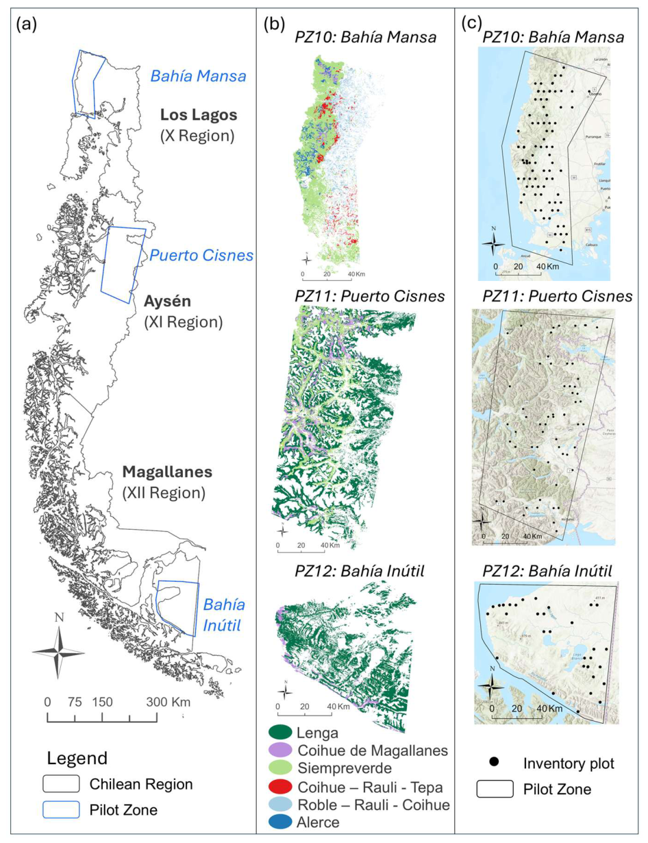
Three pilot zones (ZP) each spanning 10,000–18,000 km², were selected in Los Lagos, Aysén, and Magallanes regions (Chile). These areas include ecologically significant forest types, such as Lenga, Siempreverde, and Coihue de Magallanes (Figure 1,

Table 2. Dominant forest types and proportion of area occupied in the pilot zones.

Pilot Zone	Forest Type	% Area
PZ10: Bahía Mansa 10,353 ha	Siempreverde	64.0
	Roble-Rauli-Coihue	19.6
	Coihue-Rauli-Tepa	7.2
	Alerce	6.4
	Coihue de Magallanes	2.7
	Lenga	2.0
PZ11: Puerto Cisnes 17,839 ha	Lenga	65.0
	Siempreverde	23.0
	Coihue de Magallanes	11.0
PZ12: Bahía Inútil 13,843 ha	Lenga	94.0
	Coihue de Magallanes	6.0

). Los Lagos is dominated by wet temperate rainforests of diverse evergreen broadleaves occurring from sea level up to 1000 m a.s.l. In contrast, the colder climates of Aysén (0–2177 m) and Magallanes (0–1676 m) are dominated by Lenga forests adapted to subantarctic conditions. Within these zones, CNFI plots provided field data on forest composition, volume, and growth for algorithm calibration and accuracy assessment. Altogether, the three pilot zones cover ~42,000 km² in southern Chile (Figure 1).

2.1. Dominant Forest Types in the Pilot Zones

Forest types were characterized using vector layers from the CONAF Native Forest Cadastre. Cadastre update dates differ among Chilean regions; for the three regions considered in this study, the 2013 Cadastre represented the temporally closest available cartographic information to the 2010 PALSAR reference year and was therefore used. Across the three pilot zones, the dominant types are Lenga, Siempreverde, and Coihue de Magallanes, complemented by less extensive formations (Figure 1, Table 2).

In PZ12 (Bahía Inútil, Magallanes), Lenga dominates, forming a mosaic of woodland, scrub, and grassland shaped by harsh climate and historical fires set in the late 19th–early 20th century to create pasture [35]. In PZ11 (Puerto Cisnes, Aysén), Lenga is again the prevailing species, occupying hills and mountains as tall, dense stands [36], sometimes intermixed with Siempreverde [37,38]. Within this zone, Coihue de Magallanes dominates the rain-soaked coastal slopes, while Lenga is more common on drier inland sites. Siempreverde, covering about 23% of the area, occupies valleys and fjords, forming a mosaic of evergreen and deciduous forests. PZ10 (Bahía Mansa, Los Lagos) is the most diverse of the pilot zones. It is primarily dominated by Siempreverde within the coastal Valdivian forest but also contains several mixed forest types. Roughly half of the original forest cover has been lost or fragmented, yet extensive tracts of old-growth forest remain. Roble–Raulí–Coihue, a structurally variable Nothofagus deciduous forest that contributes nearly 45% of Chile’s native timber production, covers 19.6% of this zone. Other forest types include Coihue–Raulí–Tepa on productive Andean sites and Lenga at highest elevations.

Alerce (Fitzroya cupressoides), endemic to Chile and Argentina, is particularly notable for its longevity (>3600 years) and massive trunks (>4 m diameter) [39]. In PZ10, it occurs in both coastal and Andean sectors. Once heavily exploited for its highly durable timber, especially for shingles, Alerce populations declined drastically, and the species is now strictly protected under CITES Appendix I [8].

2.2. Field Inventory Plot Data

Data from the CNFI were provided by INFOR (Figure 1c) and include plot location, forest type, standing volume (m³·ha⁻¹), and annual growth factors per hectare. These growth factors were derived from field measurements and 10–15 years of increment-cores, providing estimates of the mean annual volume increment. The spatial distribution of inventory plots in the pilot zones (Figure 1c) reflects accessibility constraints: in PZ10, plots are relatively evenly distributed, whereas in PZ12 they concentrate along the coast and central lowlands, leaving steeper zones underrepresented. In PZ11, although the Siempreverde forest extends from sea level up to 1100 m (occasionally 1700 m), all inventory data are from below 500 m.

2.2.1. Temporal Distribution of Plot Measurements

Permanent plots are repeatedly measured with a variable revisit interval which varies by pilot zone and specific plots. In PZ10 plots measurements date back to 2001, with subsequent re-measurements in 2015 and 2019. In PZ11, plots were first measured in 2008 and remeasured in 2017–2018. In PZ12, field campaigns were conducted in 2009, 2014, and 2017–2018.

Table 3. Temporal distribution of field plots by pilot area.

Pilot Zone	Year	Number of Plots
PZ10: Bahía Mansa (Los Lagos)	2001	116
	2015	67
	2019	42
PZ11: Puerto Cisnes (Aysén)	2008	77
	2017	107
	2018	24
PZ12: Bahía Inútil (Magallanes)	2009	26
	2014	29
	2017	8
	2018	26

summarizes the temporal measurement of field plots by pilot area.

All plot volumes were projected to reference year 2010 using annual growth increments, accounting for differences in measurement dates. This provided the best estimates for temporal comparison and alignment with remote sensing acquisition dates.

2.2.2. Representativeness and Quality of Inventory Plots

The representativeness of the field data was evaluated according to forest type, spatial distribution, and stand volume.

Table 4. Distribution of inventory plots by forest type and pilot area after quality control.

Forest Type	PZ12 Bahía Inútil	PZ11 Puerto Cisnes	PZ10 Bahía Mansa
Lenga	48	112
Coihue de Magallanes	8	15
Siempreverde		30	95
Roble–Raulí–Coihue			48
Alerce			17
Coihue–Raulí–Tepa			23

summarizes the number of inventory plots retained for modelling after quality control and spatial filtering procedures.

The CNFI employs a two-stage clustered sampling design, with each sampling unit comprising three concentric circular plots of 500 m² each, distributed on a systematic 5 × 7 km grid [40]. When intersected with the 25 m ALOS PALSAR mosaics, several inventory subplots often fell within the same SAR pixel. In some cases, these plots showed large differences in stand volume despite sharing an identical radar response, reflecting forest heterogeneity at scales below the SAR spatial resolution.

To reduce plot-to-pixel inconsistencies, field observations located within the same SAR pixel that showed strongly contrasting stand-volume values were excluded from the modelling dataset, as such observations were considered insufficiently representative of a unique pixel-level remote-sensing response [16,41]. Because a single SAR pixel represents an area-averaged radar response, it cannot reliably support multiple, substantially different volume measurements. Retaining such cases would create conflicting training samples and reduce the ability of the k-NN algorithm to establish robust relationships between SAR backscatter and forest volume. Although the filtering reduced the total number of available plots, it improved the consistency between field observations and SAR pixel responses, which is particularly important when using medium-resolution radar mosaics for k-NN estimation.

After filtering, Lenga remained the most represented forest type overall, particularly in the southern pilot zones, with 48 plots in PZ12 (Bahía Inútil) and 112 plots in PZ11 (Puerto Cisnes). Coihue de Magallanes was represented by 8 plots in PZ12 and 15 plots in PZ11. In PZ10 (Bahía Mansa), Siempreverde was the dominant forest type in the inventory dataset (95 plots), followed by Roble–Raulí–Coihue (48 plots), Coihue–Raulí–Tepa (23 plots), and Alerce (17 plots). Siempreverde was also represented in PZ11 with 30 plots. This final distribution of plots conditioned both the feasibility of model calibration for each forest type and the robustness of the resulting estimations.

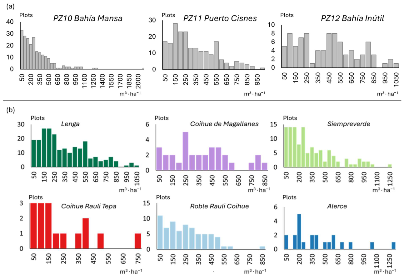
To explore volume patterns by forest type, we analysed the distribution of stand volume per hectare across field plots. Distinct trends emerge in each pilot zone (Figure 2) reflecting differences in management history and natural disturbance regimes.

In PZ10 (Bahía Mansa) the distribution shows an inverted-J shape, typical of managed forests: many plots with low to moderate volumes and progressively fewer at higher levels. Most represent young regrowth or recently harvested areas, and a few reach extremely high (>1000 m³·ha⁻¹) volumes. This long tail of very high values suggests a landscape dominated by intermediate stands interspersed with rare old-growth or highly productive patches. The prevalence of low-volume plots reflects recurring harvest-replant cycles that limit the development of old-growth conditions. In PZ11 (Puerto Cisnes), volumes follow a right-skewed distribution. Moderate-volume stands are common, but high-volume ones are increasingly rare, reaching up to ~960 m³·ha⁻¹. This pattern is consistent with largely natural forests where self-thinning maintains many stands at intermediate volumes. The scarcity of very high volumes may reflect past selective logging of largest trees. In PZ12 (Bahía Inútil), volumes show no dominant frequency peak; values are evenly distributed from low to high. This irregular pattern reflects a heterogeneous mosaic of sparse stands, dense second growth, and mature forests. Maximum volumes (~1037 m³·ha⁻¹) are substantial but below the extremes of PZ10. The absence of a dominant peak highlights the structural diversity of this zone, where young and old stands coexist in a non-uniform way.

Plot volumes grouped by forest type also exhibit some clear patterns (Figure 2b). Lenga and Coihue de Magallanes forests display distributions typical of largely natural stands, with few intermediate volumes and some very high, old-growth values. Siempreverde and Roble–Raulí–Coihue plots, by contrast, show an inverted J pattern characteristic of managed stands. Coihue–Raulí–Tepa and particularly Alerce plots lack certain volume classes, likely reflecting natural disturbances or past overexploitation. Summary statistics for each type are provided in

Table 5. Characterization of volumes per hectare in inventory plots.

Forest Type	Minimum (m3·ha−1)	Maximum (m3·ha−1)	Average (m3·ha−1)
Lenga	1.43	1037.19	325.12
Coihue de Magallanes	6.62	819.30	345.56
Siempreverde	2.51	2074.82	327.89
Coihue–Raulí–Tepa	19.41	705.00	209.88
Roble–Raulí–Coihue	1.77	837.29	229.76
Alerce	10.67	1261.61	394.17

.

2.3. ALOS PALSAR Data

ALOS-1 PALSAR-1 (2006–2011) operated at ~23.6 cm wavelength with multiple acquisition modes, full polarimetry capacity and a 46-day revisit cycle [42]. For southern Chile around 2010, it was virtually the only SAR source capable of reliably capturing forest structure. Current alternatives such as Sentinel-1 (C-band, launched April 2014) or TerraSAR-X (X-band, launched June 2007) lacked temporal coverage and L-band penetration, while L-band missions such as BIOMASS (launched in April 2025) and NISAR (launched in July 2025) were not yet operational at the time of analysis [43,44]. ALOS-1 and its successor ALOS-2 have since provided the global L-band coverage underpinning biomass mapping, particularly in remote regions (Table 1). The dual-polarization (HH, HV) configuration used over land areas enables the derivation of indices, such as the HH/HV ratio, which are sensitive to canopy density and tend to saturate at higher biomass levels than single-polarization backscatter [45]. ALOS-1 PALSAR-1 data are openly available through repositories such as the Alaska Satellite Facility (ASF, https://asf.alaska.edu, accessed on 29 December 2025).

PALSAR Annual Mosaics

JAXA provides annual global PALSAR mosaics composites of multiple acquisitions, available for 2007–2010 (ALOS-1) and from 2015 onward (ALOS-2). These mosaics provide orthorectified and radiometrically slope-corrected L-band backscatter (γ⁰) in HH and HV polarizations on a 25 m grid. Freely accessible through platforms such as Google Earth Engine and JAXA’s ALOS portal, the mosaics facilitate large-scale forest monitoring by overcoming gaps in scene availability and providing consistent, wall-to-wall coverage. Their standardized format, systematic acquisition strategy, and temporal consistency make them particularly suitable for regional biomass mapping and carbon accounting applications [46]. However, transforming these observations into reliable biomass estimates remains challenging, especially in heterogeneous and high-biomass forests where signal saturation, limited field calibration data, and environmental variability introduce substantial uncertainties. We used the JAXA Version 2 PALSAR/PALSAR-2 global mosaics available at the time of analysis, which incorporate significantly improved geolocation accuracy and refined radiometric balancing between adjacent paths relative to the earlier Version 1 products [47]. For the present analysis, the 2010 annual mosaic was used to match the common reference year of the temporally harmonized field observations.

The mosaic backscatter values, provided in digital number (DN) form, were converted to physical σ⁰ values (in decibels) using the calibration factor recommended in JAXA documentation [47].

$${\gamma }_{dB}^0=10\log {DN}^2+CF$$

(1)

With CF = −83.0 dB. We applied this conversion to all mosaic data so that the pixel values represent σ⁰ in dB. After calibration, additional derived layers were computed: the HH/HV ratio expressed in decibels (dB), calculated as the difference between HH and HV backscatter in dB, and the Radar Forest Degradation Index (RFDI), introduced by Saatchi et al. (2011) [48] and subsequently applied by Mitchard et al. (2012) [49], which is defined as:

$$RFDI={\displaystyle \frac{HH-HV}{HH+HV}}$$

(2)

with HH and HV expressed in linear power units.

This index relating intensity values emphasizes the contrast between double-bounce scattering, which increases HH returns, and volume scattering, which dominates HV returns. RFDI values range from 0 to 1 (sometimes rescaled to 1–9) and are effective for distinguishing forest conditions and disturbance levels. Higher RFDI typically reflects greater trunk-ground double bounce in sparse or degraded forests, while low values indicate dominant volume scattering in dense, closed-canopy forests [50].

2.4. Modelling Volume and Derived Carbon Stock

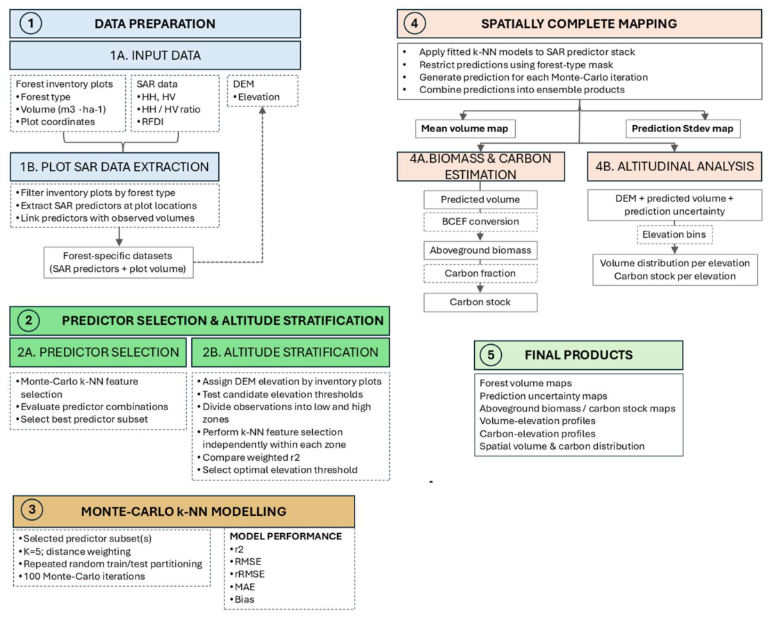
The main methodological workflow, from the integration of field inventory and SAR data to forest-volume modelling, spatial prediction, and carbon-stock estimation, is summarized in Figure 3.

2.4.1. Dependent Variable: Aboveground Volume and Carbon Stock

Forest inventory plots typically provide tree height and diameter measurements, from which stem volume is estimated and scaled to a per-hectare basis using expansion factors. In this study, stand volume was selected as the target variable because it is directly derived from the field inventory data and can be robustly related to SAR backscatter. Carbon stock was subsequently estimated from predicted volume using a Biomass Conversion and Expansion Factor (BCEF) approach following IPCC guidelines [51]. Unlike conventional methods that apply biomass expansion factors (BEF) and wood density separately, the BCEF method uses a single coefficient to convert stem volume directly into aboveground biomass. Because BCEF values vary with stand volume, they capture changes in forest structure along biomass gradients, providing a more realistic representation of biomass allocation across diverse types and wide productivity ranges.

In this framework, aboveground biomass (AGB) is estimated as:

$$AGB =V\times BCEF$$

(3)

And carbon stock is then computed as:

$$C =AGB\times CF$$

(4)

where V is stem volume (m³·ha⁻¹), BCEF is the biomass conversion and expansion factor (Mg·m⁻³), CF is the carbon fraction of dry biomass (assumed to be 0.5 following IPCC defaults).

BCEF values were assigned dynamically based on predicted volume classes and forest type, using standard tabulated coefficients for temperate forests provided in the 2006 IPCC Guidelines for National Greenhouse Gas Inventories [51]. For this purpose, forest types were grouped into hardwoods and conifers, with Alerce treated as a conifer type and all other forests as hardwoods, consistent with the classification used in the BCEF tables. The BCEF values and corresponding growing-stock volume classes used in the calculations are reported in

Table A4. Biomass conversion and expansion factors (BCEF) applied in the conversion of growing-stock volume to above-ground biomass and subsequent estimation of carbon stock. BCEF values are IPCC default values for temperate forests [51].

Forest Group	Forest Type	Stock Volume (m3·ha−1)	BCEF
Hardwoods	Lenga, Coihue de Magallanes, Siempreverde, Coihue–Raulí–Tepa, Roble–Raulí–Coihue	<20	3.00
		20–40	1.70
		41–100	1.40
		101–200	1.05
		>200	0.80
Other conifers	Alerce	<20	3.00
		20–40	1.40
		41–100	1.00
		101–200	0.75
		>200	0.70

.

Although aboveground biomass is computed as an intermediate variable, the analysis focuses on carbon stock as the final output, which is directly relevant for greenhouse gas inventories and MRV systems (Measurement, Reporting and Verification).

2.4.2. Target Dates for Modelling

To account for differences in the measurement years of field plots, stand volume (m³·ha⁻¹) for each plot was projected to the reference year 2010 using the annual volume increment associated with that inventory record. For plots measured before 2010, the annual increment was added according to the number of years between the measurement and the reference year, whereas plots measured after 2010 were back-projected by subtracting the corresponding annual increment. Thus, the projected volume was calculated as

$$V_{2010}=V_m+\left(Y_m-2010\right)I$$

(5)

where Vm is the measured plot volume, Y_m is the year of measurement, and I is the annual volume increment associated with the plot. This procedure assumes a constant annual volume increment over the projection interval and therefore does not explicitly account for temporal variations in growth or disturbances occurring between the field measurement and the reference year.

2.4.3. Predictor Variables from SAR Imagery

Predictor variables included HH and HV backscatter coefficients, the HH/HV ratio, and the Radar Forest Degradation Index (RFDI), all derived from L-band SAR mosaics of Japan’s ALOS PALSAR satellite.

To construct the feature space for the k-NN models, we evaluated combinations of these variables together with low-order interaction and polynomial terms (up to third order) such as HH²·RFDI or HV²·HH/HV. To limit model complexity and reduce overfitting, each model was restricted to a maximum of four predictors.

Preliminary analyses showed that individual SAR metrics provided limited predictive power, reflecting the non-linear relationship between radar backscatter and forest volume. Therefore, combinations of SAR variables and low-order interaction terms were explored to better capture canopy structural variability and scattering processes. Predictor selection was performed separately for each forest type and, where applicable, altitudinal stratum using a greedy forward-selection procedure. At each step, candidate predictor subsets were evaluated through repeated Monte Carlo train–test splitting, and the predictor yielding the highest mean test squared Pearson correlation coefficient (r²) was selected. To constrain model complexity relative to the available number of reference observations, a maximum of four predictors was retained. Consequently, the final predictor combinations differed among forest types and strata and are reported in

Table A1. Predictor combinations used in the final k-NN models by pilot zone, forest type, and altitudinal subset.

Pilot Zone	Forest Type	Altitude: In PZ In Plots	Num. of Samples	Final Predictors
PZ10	Alerce	0–1100 410–870	19	HH2 ∙ Ratio10, HH2
	Siempreverde	0–1100 0–727	104	HV2 ∙ Ratio, HH ∙ Ratio
		0–300 8–290	59	HV2 ∙ Ratio, Ratio ∙ RFDI, HH ∙ HV, Ratio3
		300–1100 361–727	45	Ratio3
	Coihue–Raulí	0–1000 16–490	27	HH2 ∙ Ratio
		0–200 16–198	18	HV ∙ Ratio ∙ RFDI
		200–1000 279–490	9	RFDI3, Ratio, HH ∙ RFDI, Ratio2
	Roble–Raulí	0–900 13–408	52	HV2 ∙ RFDI, HH ∙ Ratio ∙ RFDI, HH ∙ HV ∙ RFDI HH ∙ RFDI
		0–200 13–176	26	HH ∙ HV ∙ RFDI, HV2
		200–900 211–408	26	HH
PZ11	Siempreverde	0–1900 28–478	32	HH ∙ HV ∙ RFDI
	Coihue de M.	0–1500 187–820	15	HH ∙ HV ∙ Ratio
	Lenga	0–1700 305–1178	140	HH ∙ Ratio ∙ RFDI, Ratio ∙ RFDI2, HH ∙ RFDI, HV ∙ RFDI2
		0–700 305–660	52	HH ∙ HV2, HH2 ∙ Ratio
		700–1700 700–1180	88	HV ∙ RFDI2, Ratio, RFDI2, RFDI3
PZ12	Coihue de M.	0–800 27–118	10	HV ∙ RFDI, HV ∙ Ratio ∙ RFDI
	Lenga	0–1100 53–517	60	HH ∙ HV ∙ Ratio

.

Plot locations were intersected with the SAR rasters to extract predictor values, generating a training dataset that linked field-estimated stand volume (dependent variable) with SAR-derived metrics for each forest type and ZP.

2.4.4. Modelling Method: k-NN Regression

Forest volume was estimated from SAR predictors using k-Nearest Neighbors (k-NN) regression. k-NN was selected because it is a well-established non-parametric method that has been extensively applied to combine forest-inventory observations with spatially exhaustive remotely sensed data, including in operational national forest inventories [52]. This non-parametric method does not require assumptions about variable distributions, making it well-suited to the skewed and heteroscedastic characteristics of forest volume and SAR backscatter data [52,53]. Rather than fitting a global model, k-NN predicts volume based on feature similarity: for each 25 m pixel, the algorithm identifies the k training plots with the most similar predictor values and estimates volume as the weighted average of their measured volumes. The predictor space was defined by the selected combination of SAR-derived variables and their transformations for each model.

The choice of k = 5 represented a compromise between model performance and the markedly different reference sample sizes among forest-type and pilot-zone datasets. A sensitivity analysis using k = 3, 5, and 7 for two comparatively well-sampled datasets (Lenga in PZ11, n = 140, and PZ12, n = 60) showed only minor differences in validation performance across this range (

Table A2. Sensitivity of k-NN validation performance to the number of neighbours (k) for Lenga in PZ11 and PZ12.

Pilot Zone	Forest Type	Num. of Samples	r2	k	MAE (m3·ha−1)	RMSE (m3·ha−1)
PZ11	Lenga	140	0.11	3	155.56	155.56
			0.12	5	150.93	150.93
			0.12	7	151.05	51.05
PZ12	Lenga	60	0.45	3	157.39	157.39
			0.47	5	156.40	156.40
			0.48	7	156.65	195.60

). Higher values of k were not considered appropriate as a common setting because several forest-type datasets contained substantially fewer reference observations and consequently small training subsets. Distance weighting was applied so nearer neighbours had greater influence, using Euclidean distance in the four-dimensional spectral space ($w_i={\displaystyle \frac{1}{{|\left|x-x_i|\right|}_2}},$where the subscript 2 means the L2 Euclidean norm). Predictors were normalized to avoid dominance by differing scales. The scaler used is given by the equation:

$$x_{scaled}= ={\displaystyle \frac{x-median}{IQR}}$$

(6)

where IQR = Q3 − Q1, Q1 is the 25th percentile, and Q3 is the 75th percentile.

The k-NN models were implemented in Python (version 3.13.5) using the KNeighborsRegressor implementation in scikit-learn. Predictor scaling was performed within the modelling pipeline and fitted independently to the training subset in each Monte Carlo iteration, thereby preventing information from the corresponding test subset from entering the scaling procedure. Zero-distance cases were handled according to the standard scikit-learn distance-weighting implementation.

The data were randomly partitioned into training (80%) and test (20%) subsets in multiple Monte Carlo runs; however, in cases where inventory data were particularly scarce, a 70–30% split was adopted to ensure a sufficient number of observations for model validation. Different splits were generated by using a unique random seed for each run. A total of 100 runs were performed, yielding a distribution of performance metrics that enabled a robust estimation of average model accuracy and its variability.

For forest types with broad altitudinal distributions, an altitude-stratified approach was also evaluated. Candidate elevation thresholds were used to divide inventory observations into two strata, with further subdivision precluded by sample-size limitations. Separate k-NN models were fitted and evaluated for each stratum using the same Monte Carlo procedure as for the complete datasets. The threshold maximizing the sample-size-weighted mean test r² across both strata, subject to a minimum sample size per stratum, was retained.

2.4.5. Model Validation and Accuracy Assessment

Model accuracy was reported using several error metrics. Mean Absolute Error (MAE) and Root Mean Square Error (RMSE) were computed for training and test data. In addition, the squared Pearson correlation coefficient (r²) was evaluated for both training and test sets. To facilitate comparison among forest types with different mean stand volumes, relative RMSE (rRMSE) was calculated using the mean test RMSE across the Monte Carlo iterations and mean observed volume of the corresponding modelling dataset. For restricted-volume analyses, the mean observed volume of the corresponding restricted dataset was used (

Table A3. Additional validation statistics for the k-NN models by pilot zone, forest type and modelling stratum. Relative root mean square error (rRMSE) was calculated by normalizing the mean test RMSE reported in Table 6 by the mean observed stand volume of the corresponding modelling dataset. Bias represents the mean prediction error across the Monte Carlo test subsets.

Pilot Zone	Altitude: In PZ In Plots	Inventory Volumes (Subset)		rRMSE (%)	Bias (m3·ha−1)
Alerce
PZ10	0–1100 410–870	29–812	19	49.01	−31.96
Siempreverde
PZ10	0–1100 0–727	9–2190	104	97.72	6.99
	0–300 8–290	10–2190 (10–900)	59	100.85	8.02
	300–1100 361–727	9–1350 (9–900)	45	70.32	47.69
PZ11	0–1900 28–478	65–879 (65–400)	32	61.29	−1.68
Roble–Raulí–Coihue
PZ10	0–900 13–408	2–755 (2–250)	52	95.86	1.54
	0–200 13–176	7–755 (7–250)	26	92.18	−3.42
	200–900 211–408	2–567 (2–250)	26	90.17	16.57
Coihue–Raulí–Tepa
PZ10	0–1000 16–490	25–702 (25–400)	27	86.09	−6.05
	0–200 16–198	55–674 (55–400)	18	83.20	1.23
	200–1000 279–490	25–702 (25–400)	9	66.34	31.67
Coihue de Magallanes
PZ11	0–1500 187–820	26–773 (26–500)	15	48.39	76.63
PZ12	0–800 27–118	175–807 (175–600)	10	20.93	−9.38
Lenga
PZ11	0–1700 305–1178	5–918 (5–350)	140	73.22	−7.87
	0–700 305–660	5–918 (350)	52	79.69	−13.34
	700–1700 700–1180	7–720 (350)	88	65.99	−2.21
PZ12	0–1100 53–517	3–1044 (3–450)	60	52.40	11.07

).

The test observations were withheld from model fitting within each Monte Carlo iteration and therefore provided repeated out-of-sample evaluation. However, these observations are referred to as held-out test subsets rather than as an independent validation dataset because random partitioning was used and spatial dependence between training and test observations was not explicitly assessed. Moreover, because predictive performance on the Monte Carlo test subsets was used during predictor selection, these subsets do not constitute an untouched final validation dataset. The reported test statistics should therefore be interpreted as internal model-selection and hold-out performance estimates rather than as fully independent estimates of generalization error.

2.4.6. Comparison with Random Forest

To evaluate whether the choice of k-NN constrained model performance, an additional comparison was conducted using Random Forest (RF). Rather than repeating the comparison for all forest-type and pilot-zone combinations, the analysis focused on Lenga in PZ11 (Aysén) and PZ12 (Magallanes), which provided the largest and one of the next-largest reference datasets available for an individual forest type (n = 140 and n = 60, respectively). This avoided basing the algorithm comparison on forest types represented by very small reference samples. The two Lenga datasets also provided contrasting k-NN validation performance, with test r² values of 0.12 in PZ11 and 0.47 in PZ12.

RF was first evaluated using the same predictor sets selected for the corresponding k-NN models, thereby allowing a direct comparison of the modelling algorithms while holding the input information constant. The same Monte Carlo train–test partitions were used for both algorithms. As an additional test, RF was also evaluated using the four basic SAR predictors (HH, HV, HH/HV ratio and RFDI) to assess whether access to the untransformed predictor set improved RF performance. Model performance was compared using test r², RMSE and MAE averaged across the 100 Monte Carlo runs.

2.4.7. Volume and Carbon Stock Mapping

An advantage of k-NN modelling is its straightforward extension to wall-to-wall mapping: once trained, the algorithm can be applied pixel by pixel to generate continuous maps of the variable of interest [52]. After validation, the k-NN models were applied wall-to-wall to produce forest volume maps. To ensure that each model was applied only to its corresponding forest type, the CONAF vector forest-type layers were rasterized at a spatial resolution of 25 × 25 m to generate the modelling masks. Rasterization used a pixel-centre criterion: a pixel was assigned to a forest-type polygon only when its centre fell within that polygon; pixels whose centres fell outside the polygon were excluded, irrespective of the proportion of the pixel intersected by the polygon. The resulting masks and the ALOS PALSAR predictor stacks were co-registered and spatially aligned, ensuring a common grid for wall-to-wall prediction. Pixels outside the corresponding forest-type mask were treated as background and excluded from prediction.

Additional variables of interest, such as carbon stock, were derived using raster algebra at a 25 m pixel resolution. Values were summarized by altitude using the 30 m SRTM void-filled dataset covering the pilot zones, obtained from EarthExplorer (USGS).

Spatial prediction variability was characterized using the pixel-wise standard deviation (SD) of the estimates across the Monte Carlo model realizations. The resulting SD maps characterize variability associated with the k-NN prediction process and do not include uncertainty in the BCEF coefficients, carbon fraction, temporal projection of inventory measurements, or field observations.

3. Results

3.1. Statistical Results

Modelling Performance

The k-NN models showed moderate to high predictive capacity across forest types and pilot zones, although performance varied depending on forest structure, sample size, and the environmental representativeness of the inventory plots. Model evaluation was performed using Monte-Carlo cross-validation, producing distributions of r², RMSE and MAE for each forest-type model.

Table 6. Summary of the k-NN models’ results in the three pilot zones.

Pilot Zone	Altitude: In PZ In Plots	Plots Volume (Subset)	r2 Train/Test (Subset)	MAE Train/Test (Subset)	RMSE Train/Test (Subset)	Num. of Samples
Alerce
PZ10	0–1100 410–870	29–812 (29–550)	0.99/0.63 (0.72)	4.66/149.16 (128.62)	12.65/177.81 (150.45)	19
Siempreverde
PZ10	0–1100 0–727	9–2190 (9–900)	0.99/0.26 (0.33)	5.24/196.67 (161.40)	17.71/290.60 (217.12)	104
	0–300 8–290	10–2190 (10–900)	0.99/0.41 (0.43)	4.00/185.67 (148.87)	15.07/270.27 (187.70)	59
	300–1100 361–727	9–1350 (9–900)	0.99/0.46 (0.55)	6.54/172.62 (145.92)	19.01/236.20 (184.99)	45
PZ11	0–1900 28–478	65–879 (65–400)	0.98/0.26 (0.49)	7.45/161.47 (130.76)	25.54/201.19 (158.65)	32
Roble Raulí-Coihue
PZ10	0–900 13–408	2–755 (2–250)	0.96/0.14 (0.17)	10.41/178.54 (142.39)	30.72/209.18 (164.07)	52
	0–200 13–176	7–755 (7–250)	1.00/0.38 (0.47)	0/186.70 (147.03)	0/226.50 (172.59)	26
	200–900 211–408	2–567 (2–250)	0–92/0.26 (0.40)	19.84/152.51 (140.27)	41.79/179.65 (164.17)	26
Coihue Raulí-Tepa
PZ10	0–1000 16–490	25–702 (25–400)	0.87/0.18 (0.27)	24.84/203.79 (169.80)	57.32/239.84 (197.37)	27
	0–200 16–198	55–674 (55–400)	0.84/0.30 (0.37)	31.66/147.61 (122.79)	64.03/192.02 (158.93)	18
	200–1000 279–490	25–702 (25–400)	1.00/0.76 (0.94)	0/161.50 (155.66)	0/195.30 (164.23)	9
Coihue de Magallanes
PZ11	0–1500 187–820	26–773 (26–500)	1.00/0.70 (0.87)	0/152.92 (154.81)	0/175.49 (170.35)	15
PZ12	0–800 27–118	175–807 (175–600)	0.99/0.90 (0.92)	7.01/85.13 (62.61)	12.16/98.37 (71.51)	10
Lenga
PZ11	0–1700 305–1178	5–918 (5–350)	0.84/0.12 (0.17)	31.41/151.19 (115.15)	73.00/196.85 (152.19)	140
	0–700 305–660	5–918 (350)	0.93/0.30 (0.28)	17.05/109.10 (74.47)	44.00/159.18 (105.53)	52
	700–1700 700–1180	7–720 (350)	0.79/0.10 (0.17)	38.15/159.94 (131.52)	82.64/204.09 (164.92)	88
PZ12	0–1100 53–517	3–1044 (3–450)	0.97/0.47 (0.41)	17.04/156.40 (135.37)	43.58/197.30 (164.47)	60

summarizes the results for the different pilot zones, forest types, and altitude configurations.

Training r² values were generally high (0.84–1.00) whereas test r² values range from approximately 0.12 to 0.90, with most models falling between 0.18 and 0.63. The gap between training and validation performance indicates varying degrees of overfitting, particularly in forest type-PZ combinations with limited inventory data (e.g., Coihue de Magallanes in PZ’s 11 and 12). In these cases, the models captured patterns specific to the training set but generalized less effectively to the held-out test subsets.

Sensitivity tests for two comparatively well-sampled Lenga datasets showed limited sensitivity to the number of neighbours over k = 3–7 (Table A2). In PZ11, test r² ranged from 0.11 to 0.12 and RMSE from 196.07 to 201.69 m³·ha⁻¹, while in PZ12, r² ranged from 0.45 to 0.48 and RMSE from 195.60 to 201.69 m³·ha⁻¹.

Model performance was partly influenced by strong environmental gradients, particularly altitude, which affect forest structure, species composition, and productivity. In several cases, stratifying the data by altitude improved predictive accuracy. For example, in Siempreverde forests of PZ10, the overall model achieved a test r² of 0.26, whereas separate models for lower and higher altitude zones increased test r² to 0.41 and 0.46, respectively. Similarly, in Coihue–Raulí forests of PZ10, test r² improved from 0.18 for the overall model to 0.30 and 0.76 for the lower- and higher-altitude subsets. Comparable improvements were observed for Roble–Raulí forests. These results indicate that stratification along major ecological gradients can reduce within-group heterogeneity and enhance model performance. Nevertheless, stratification also reduces the number of available training plots, which in some cases increased overfitting, particularly in subsets with limited sample sizes.

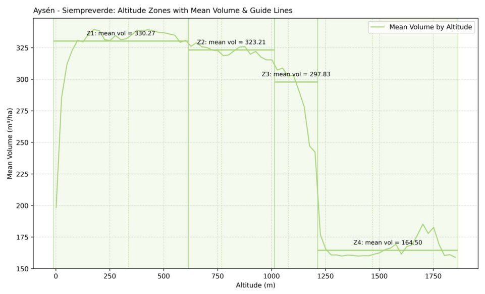
A consistent pattern emerged when model performance was evaluated for lower stand-volume ranges. Although models were calibrated using the full range of observed volumes, additional validation statistics were calculated for plots below specific volume thresholds (shown in brackets in Table 6). Within these restricted ranges, models generally showed lower errors and higher r² values than those obtained across the full volume spectrum. For example, test r² increased from 0.63 to 0.72 in Alerce forests and from 0.26 to 0.49 in Siempreverde forests (reaching 0.43–0.55 when combining with altitude stratification). Similar improvements were observed for Roble–Raulí forests, where test r² increased from 0.26 to 0.40 for stands above 200 m elevation and below 250 m³·ha⁻1 and for Alerce forests in PZ10 (0.63 to 0.72). Across all forest types and pilot zones, mean predicted volumes remained below the corresponding threshold values used for the restricted analyses, as shown in Figure 4.

Prediction errors were relatively high, reflecting the high natural variability in stand volume across southern Chilean forests. Test MAE values typically ranged from 100 to 200 m³·ha⁻¹, while RMSE varied from about 100 to nearly 300 m³·ha⁻¹ depending on forest type and pilot zone. These error levels are consistent with the broad volume distributions observed in the inventory data, where stand volumes often span several hundred cubic meters per hectare. The rRMSE values (Table A3) showed substantial variation among forest types and modelling strata. No consistent correspondence was observed between rRMSE and test r², reflecting the different information provided by these metrics: rRMSE quantifies prediction error relative to the mean observed stand volume, whereas r² describes the proportion of variability among observations reproduced by the model.

Model performance varied among forest types and pilot zones. In PZ10 (Los Lagos), structurally complex forest types such as Siempreverde showed lower predictive accuracy and larger errors, reflecting their high species diversity and structural heterogeneity. In contrast, Alerce forests achieved higher r² values and lower errors, although the limited number of inventory plots warrants caution in interpretation. As observed elsewhere, restricting the evaluation to lower volume ranges and stratifying by altitude generally improved model performance, although small sample sizes reduced the robustness of some stratified results.

In PZ11 (Aysén), models for Coihue de Magallanes outperformed those for Lenga. Despite having a larger number of inventory plots, Lenga forests exhibited lower r² values and higher prediction errors, indicating that ecological variability played a greater role than sample size. The broader ecological range occupied by Lenga, particularly across altitude gradients, likely contributed to this lower performance. For Siempreverde forests, the available plots were restricted to altitudes below 500 m, preventing meaningful altitude stratification despite the species occurring up to approximately 1800 m a.s.l. Nevertheless, model performance improved when evaluation was limited to volumes below 400 m³·ha⁻¹ m³·ha⁻¹.

In PZ12 (Magallanes), models showed moderate predictive performance, with results varying by forest type and data availability. As in other pilot zones, evaluations restricted to lower-volume ranges generally produced lower prediction errors and improved fit, suggesting greater model stability where SAR signal remained sensitive to structural variation.

Overall, model performance depended strongly on the representativeness of the inventory data across both volume and altitude gradients. While r² provides an indication of explained variance, MAE and RMSE offer a more informative measure of practical prediction accuracy in these highly heterogeneous forest ecosystems.

As an additional test of whether predictive performance was dependent on the choice of modelling algorithm, k-NN was compared with Random Forest (RF) for Lenga in PZ11 and PZ12 (

Table 7. Comparison of k-NN and Random Forest (RF) for Lenga forest in PZ11 and PZ12. Values represent mean test statistics across 100 Monte Carlo runs.

Pilot Zone	Num. of Samples	Method	Predictor Set	Test r2	MAE (m3·ha−1)	RMSE (m3·ha−1)
PZ11	140	k-NN	Selected predictors	0.12	150.93	196.66
		RF	Same predictors as k-NN	0.16	143.61	181.70
PZ12	60	k-NN	Selected predictors	0.47	156.40	197.30
		RF	Same predictors as k-NN	0.41	171.30	211.45

). These datasets were selected because they provided comparatively large reference samples (n = 140 and n = 60, respectively) while exhibiting contrasting k-NN validation performance.

RF produced different effects in the two pilot zones. In PZ11, RF moderately improved validation performance relative to k-NN, increasing test r² from 0.12 to 0.16 and reducing RMSE from 196.66 to 181.70 m³·ha⁻¹ m³·ha⁻¹. In contrast, in PZ12, k-NN performed better, with test r² of 0.47 compared with 0.41 for RF and RMSE of 197.30 compared with 211.40 m³·ha⁻¹ m³·ha⁻¹. Additional RF runs using the four basic SAR predictors (HH, HV, HH/HV ratio and RFDI) produced similar or poorer results (test r² = 0.15 and 0.34 for PZ11 and PZ12, respectively). Overall, RF did not consistently outperform k-NN across the two datasets.

3.2. Altitudinal Patterns of Forest Volume and Carbon

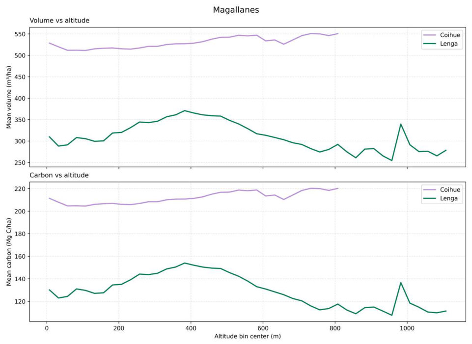
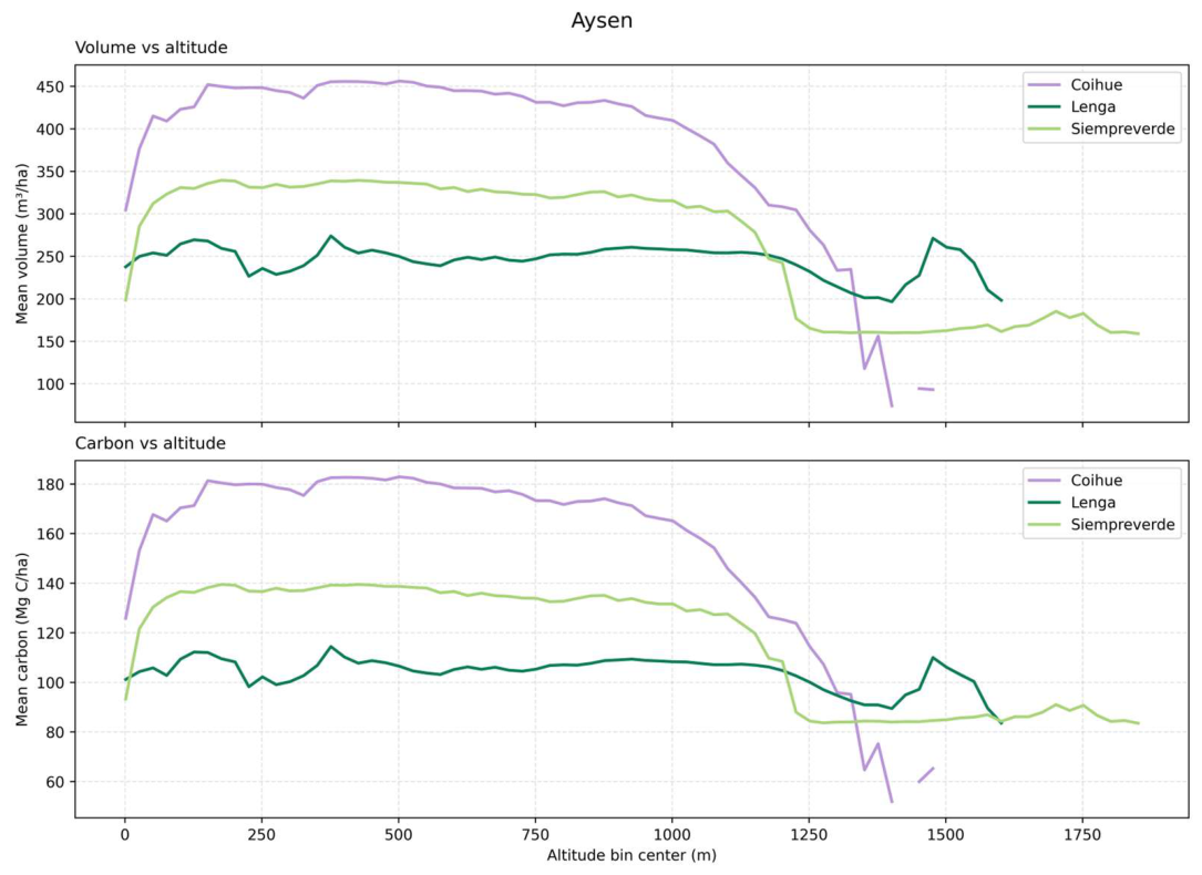
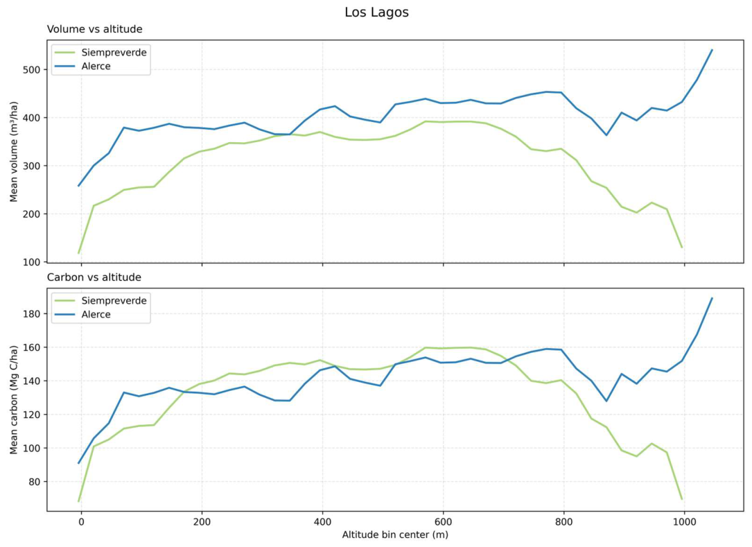
To further explore the spatial distribution of forest volume and identify elevation ranges where native forests concentrate the greatest carbon stock, predicted volume and derived carbon stocks were aggregated by elevation classes using the SRTM DEM. The resulting profiles revealed distinct altitudinal patterns among forest types and regions. Although carbon stocks generally followed the same trends as forest volume, the relationship was not strictly proportional because forest-type-specific BCEF coefficients were applied (Section 2.4.1). Differences in biomass allocation between hardwood and conifer forests therefore resulted in distinct carbon estimates for similar stand volumes.

3.2.1. Magallanes (PZ12)

In Magallanes, Coihue de Magallanes exhibits consistently high-volume values across the entire elevation gradient, with only a slight increase toward higher elevations (Figure 5). Mean volumes range approximately between 510 and 550 m³·ha⁻¹ m³·ha⁻¹, indicating structurally mature and relatively homogeneous stands.

In contrast, Lenga shows a clear unimodal distribution, with maximum volumes (~360–370 m³·ha⁻¹ m³·ha⁻¹) at mid elevations (~400 m), followed by a progressive decline toward higher altitudes (<300 m³·ha⁻¹ m³·ha⁻¹ above 800 m). This pattern may partly reflect environmental constraints like temperature and wind exposure, but is likely influenced by the limited altitudinal range of the training data (53–517 m), which affects predictions at higher elevations.

3.2.2. Aysén (PZ11)

Aysén presents more complex and fragmented patterns, as shown in Figure 6. Coihue shows high volumes at low–mid elevations (~450 m³·ha⁻¹ m³·ha⁻¹) but a strong decline above ~1000 m, dropping below 200 m³·ha⁻¹ m³·ha⁻¹. Siempreverde follows a similar pattern, peaking at ~300–400 m and decreasing sharply beyond ~1200 m. These patterns suggest the influence of strong environmental gradients, as well as limitations in the representativeness of the training data at higher elevations (with no field data above 478 m for Siempreverde and 820 m for Coihue).

Lenga exhibits relatively stable volumes across elevations (~230–270 m³·ha⁻¹ m³·ha⁻¹), with moderate variability and no strong peak, likely reflecting the low predictive performance of the k-NN model for this forest type.

3.2.3. Los Lagos (PZ10)

Los Lagos displays the most heterogeneous patterns, as shown in Figure 7. Alerce shows a strong increasing trend with elevation, reaching maximum values above 450 m³·ha⁻¹ m³·ha⁻¹ at around 800 m. However, as no field data are available above 870 m, estimates at higher elevations (>900 m) should be interpreted with caution. Siempreverde forests peak at mid elevations (~600 m) with volumes around 390 m³·ha⁻¹, followed by a marked decline at higher altitudes.

Interestingly, although Alerce exhibits higher volume values, carbon stocks are higher in Siempreverde forests due to differences in forest-type-specific BCEF coefficients. This divergence reflects ecological specialization: Alerce dominates colder, higher elevation environments, while Siempreverde forests are more productive under intermediate climatic conditions.

Roble–Raulí–Coihue and Coihue–Raulí–Tepa forest types were not included in this analysis due to their low predictive performance, which results in estimates close to the mean and limits their interpretability.

3.2.4. Volume and Carbon Stock Mapping

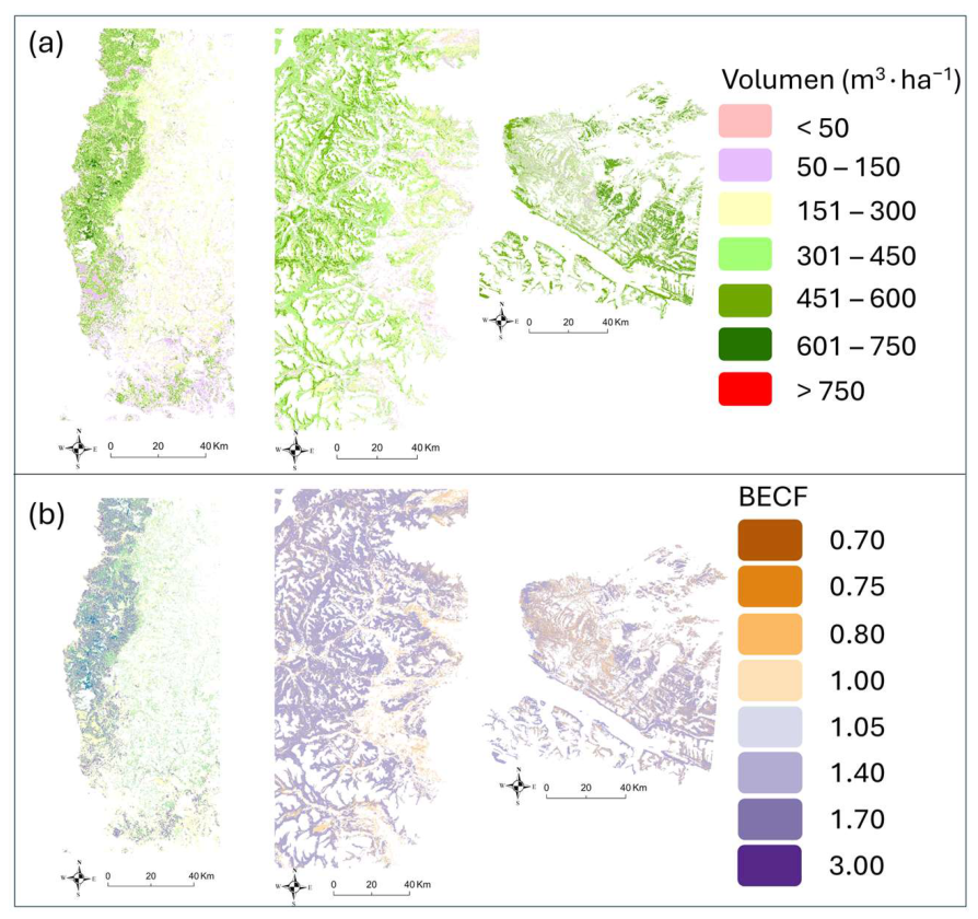
The spatial predictions show substantial within-zone heterogeneity in forest volume that is not represented by regional summary statistics alone (Figure 8). PZ10 (Los Lagos) contains extensive areas in the low- to intermediate-volume classes (<300 m³·ha⁻¹), interspersed with localized areas of higher predicted volume. In contrast, PZ11 (Aysén) shows a stronger spatial presence of the 301–450 and 451–600 m³·ha⁻¹ classes, while PZ12 (Magallanes) also contains substantial areas within these classes and localized values of 601–750 m³·ha⁻¹. The mapped BCEF values also vary spatially, reflecting their assignment according to forest category and predicted growing-stock volume class and resulting in spatially variable conversion of predicted volume to biomass and carbon stock.

Table 8. Summary of volume models with k-NN algorithm in the pilot areas.

Pilot Zone	Forest Type	Mean Volume (m3·ha−1)	Total Vol. (Mm3)	Volume Std Dev	Mean Carbon (Mg C·ha−1)	Total Carbon (Mt C)	Carbon Std Dev
PZ10	Alerce	419.25	10.81	176.51	147.10	3.79	61.28
	Siempreverde	309.30	85.90	207.52	131.68	36.57	75.95
	Coihue–Raulí	281.92	11.63	39.63	113.04	4.66	15.39
	Roble–Raulí	223.34	20.62	52.10	96.82	8.94	15.66
PZ11	Coihue de M.	437.56	40.78	112.88	175.74	16.38	43.39
	Lenga	251.12	140.65	95.41	106.41	59.60	32.14
	Siempreverde	325.48	66.67	132.76	134.91	27.63	47.17
PZ12	Coihue de M.	519.03	23.77	66.58	207.61	9.51	26.63
	Lenga	336.76	108.31	193.94	141.16	45.40	71.13

summarizes the mapped forest volume and carbon stock across the three pilot zones, highlighting substantial differences among forest types in both structural density (mean values) and total carbon storage. These differences reflect the combined influence of forest productivity and spatial extent, with some forest types exhibiting high per-hectare values but relatively low total contributions, and others dominating regional carbon stocks due to their larger spatial coverage.

In Los Lagos (PZ10), the most heterogeneous zone, Alerce forests exhibited the highest mean volume (419 m³·ha⁻¹), followed by Siempreverde (309 m³·ha⁻¹), Coihue–Raulí–Tepa (282 m³·ha⁻¹), and Roble–Raulí (223 m³·ha⁻¹). However, total carbon stocks were dominated by Siempreverde forests (36.57 Mt C), because of their much larger spatial extent. In contrast, Alerce, despite its high volume and carbon density (147 Mg C·ha⁻¹), contributed only 3.79 Mt C. Together, the mixed Roble–Raulí and Coihue–Raulí forests accounted for approximately 13.6 Mt C, highlighting their regional importance. Differences between volume and carbon patterns reflect the use of forest-type-specific BCEF coefficients, which generally yield higher carbon estimates per unit volume in hardwood forests than in conifer-dominated stands such as Alerce.

In Aysén (PZ11), Lenga forests contained the largest carbon stock (59.60 Mt C) despite only moderate mean volume (251 m³·ha⁻¹), owing to their extensive distribution. Coihue forests showed the highest mean volume (438 m³·ha⁻¹) and carbon density (176 Mg C·ha⁻¹), but their total contribution (16.38 Mt C) was limited by a smaller area. Siempreverde forests displayed intermediate values for both stand structure (325 m³·ha⁻¹; 135 Mg C·ha⁻¹) and total carbon stock (27.63 Mt C). These results illustrate how total carbon storage depends not only on stand density but also on forest extent.

In Magallanes (PZ12), Coihue forests reached the highest mean volume (519 m³·ha⁻¹) and carbon density (208 Mg C·ha⁻¹) observed across all pilot zones, indicating dense and structurally mature stands. However, Lenga forests dominated total carbon storage (45.40 Mt C) because of their much larger spatial coverage, compared with 9.51 Mt C for Coihue. As in Aysén, regional carbon stocks were driven more by forest area than by per-hectare density.

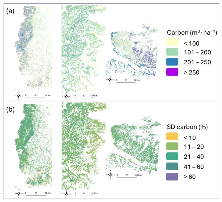
The spatial distribution of carbon stocks and prediction variability is shown in Figure 8 and Figure 9. Carbon-stock patterns broadly reflect predicted volume distributions but are modified by the forest-type- and volume-dependent BCEF coefficients (Figure 8); consequently, areas of high carbon density do not necessarily coincide with the highest predicted forest volumes. Los Lagos shows a heterogeneous distribution of carbon-stock classes, including areas of relatively high carbon density, whereas Aysén is dominated by the 101–200 Mg C·ha⁻¹ class despite its comparatively high predicted forest volumes. Magallanes shows a mixture of intermediate and higher carbon-stock classes.

Prediction variability is spatially heterogeneous within and among pilot zones (Figure 9). Nevertheless, most mapped forest falls within the two lower SD classes (≤40 Mg C·ha⁻¹), while areas with SD values of 41–60 Mg C·ha⁻¹ are more localized and those with values >60 Mg C·ha⁻¹ are comparatively limited.

Substantial within-type variability was observed across pilot zones, reflecting the high structural heterogeneity of Chilean native forests, particularly in Siempreverde and Lenga stands. Overall, model performance varied substantially among forest types and pilot zones, while the resulting maps provided spatially continuous estimates of forest volume and derived carbon stock across the three study areas. The integration of SAR observations with forest inventory data enables consistent carbon-stock estimation across heterogeneous and data-limited regions, providing information potentially relevant to Tier-3 carbon accounting and MRV applications.

4. Discussion

4.1. Model Performance and Environmental Control

Estimating forest structural variables, including biomass, using radar data poses multiple challenges [54]. Unlike the estimation of historical forest disturbances, which can rely solely on satellite data, the estimation of biophysical properties requiring calibration with field measurements introduces additional uncertainties related to both the quality and representativeness of the field data. In the present study, these uncertainties arise from sources, including uneven spatial and altitudinal distribution of inventory plots, accessibility-driven sampling biases, limited sample sizes for some forest types, and the saturation of L-band SAR signals at high biomass levels. The observed differences between training and validation results further indicate that model uncertainty remains substantial in some cases. Moreover, state-of-the-art technologies available today, such as satellite LiDAR data from GEDI, or SAR data from Sentinel-1, NISAR, or BIOMASS satellites, are unfeasible for retrospective analyses, since they were not available during the historical reference periods. Reference periods for carbon emission reporting, such as the 2001–2010 baseline established in Chile, were defined after these dates had already passed. Therefore, planning data collection in advance was not possible, and methods for estimating carbon stocks and emissions must adapt to the limitations and idiosyncrasies of the available data. Consequently, historical carbon estimates should be interpreted as approximations subject to both measurement and modelling uncertainty. Nevertheless, estimates of carbon stocks, emissions, and equivalent CO₂ fluxes remain essential components of national MRV systems and provide valuable information for greenhouse-gas reporting and climate-policy implementation.

A recent assessment incorporated forest degradation into Chile’s updated Forest Reference Emission Level/Forest Reference Level (FREL/FRL) framework [8], enabling the quantification of carbon emissions and removals not only from deforestation but also from biomass losses within permanent forests caused by degradation, wildfires, and other disturbances [8,48]. This study evaluates a retrospective mapping framework for estimating forest volume and carbon stocks by integrating National Forest Inventory data with L-band SAR imagery. By exploiting the synoptic and spatially continuous coverage of SAR imagery, the approach overcomes the limitations of sparse field observations in extensive and difficult-to-access forest landscapes.

The results demonstrate the potential of L-band SAR data to contribute to spatially explicit forest carbon accounting frameworks relevant to Tier-3 applications for retrospective estimation of forest volume and carbon stocks in southern Chile. In the persistently cloudy regions of Los Lagos, Aysén, and Magallanes, SAR imagery offers a clear advantage over optical sensors by providing consistent observations regardless of weather conditions. By combining ALOS PALSAR mosaics with Chile’s National Forest Inventory, we generated spatially explicit estimates of forest volume and carbon stocks for historical reference periods, extending inventory information across large and remote areas where field measurements are limited and optical imagery is frequently affected by cloud cover.

The integration of wall-to-wall SAR observations with inventory data produced coherent regional estimates despite the environmental heterogeneity and logistical constraints of Patagonian forests. The retrospective use of ALOS PALSAR is particularly valuable because it represents the only globally consistent L-band SAR archives available for the reference period associated with Chile’s REDD+ reference levels and conservation policies [8,55]. Similar approaches have been successfully applied at global scale by Santoro et al. [37], who combined historical L-band SAR observations with inventory data to generate spatially explicit AGB estimates for 2010, highlighting the value of historical radar archives for forest carbon accounting. Rather than replacing field inventories, the proposed methodology complements them by transforming local measurements into spatially continuous estimates, thereby strengthening forest carbon accounting and supporting MRV systems in regions where conventional monitoring remains challenging.

The continuity of the ALOS program has strengthened the operational potential of SAR-based forest monitoring. ALOS-2 PALSAR-2, launched in 2014, maintained compatibility with ALOS-1 through the use of L-band HH/HV polarizations while improving revisit frequency (14 versus 46 days) and acquisition flexibility via both ascending and descending observations. It also introduced new acquisition modes, including spotlight, stripmap, and ScanSAR, enabling observations at multiple spatial resolutions and swath widths. More recently, ALOS-4 PALSAR-3 (launched in 2024) has further enhanced coverage and observation frequency.

Since the start of this study, access to ALOS-2 products has progressively improved. Although full-resolution Stripmap and Spotlight data remain largely restricted to commercial or research agreements, annual global mosaics and an increasing number of ScanSAR products are now openly available through platforms such as JAXA G-Portal, Google Earth Engine, ASF Earthdata, and other cloud-based services. These developments greatly enhance the feasibility of long-term L-band SAR monitoring and support the extension of retrospective biomass and carbon accounting approaches beyond the original ALOS-1 era.

4.2. Limitations Related to Temporal Consistency and Field-Data Representativeness

An important limitation of this retrospective approach is the temporal mismatch between field inventory measurements and the SAR observations used for modelling (Table 3). In none of the pilot zones were field campaigns conducted concurrently with the 2010 ALOS PALSAR acquisitions; therefore, plot volumes had to be projected to the reference year (2010) using linear growth assumptions derived from inventory data and regional growth estimates. While operationally practical, this introduces uncertainty because forest growth varies with stand age, species composition, disturbance history, and climatic conditions. Consequently, projected volumes may differ from actual forest conditions at the time of SAR acquisition, particularly where the time lag between field and satellite observation is large.

The forest-type masks were based on the 2013 CONAF Cadastre, the temporally closest available cartographic information to the 2010 reference year. This three-year difference introduces potential temporal uncertainty, as forest-cover or forest-type changes during this interval could affect reconstructed forest areas and associated carbon-stock estimates. A quantitative assessment of these changes was not possible with the available historical information. Commercial forest management is largely absent from the native forests represented in PZ11 and PZ12 and is mainly relevant in PZ10; nevertheless, some mismatch between 2010 forest conditions and the 2013 forest-type masks cannot be excluded.

Additional uncertainty arises from the temporal composition of the annual ALOS PALSAR mosaics. Although metadata indicate that most study areas were covered by a limited number of acquisitions within relatively short periods (17 days in Magallanes and approximately one to two months in Los Lagos and Aysén). Some variability associated with differences in canopy moisture, precipitation, and seasonal vegetation conditions remains unavoidable.

The clustered design of Chile’s Continuous National Forest Inventory constitutes a further source of uncertainty. Accessibility constraints result in an uneven distribution of plots across environmental gradients, particularly along altitude ranges. In several cases, forests above 1000 m were represented mainly by lower-elevation plots, reducing the reliability of model extrapolation into under-sampled environments and likely contributing to prediction errors in high-altitude forests. This mismatch between the environmental conditions represented by the inventory and the full ecological range of the forests requires the models to extrapolate beyond the calibration domain. Consequently, some of the improvements observed when analyses were restricted to specific altitude or volume ranges may reflect a reduction in extrapolation rather than a true increase in model accuracy. More generally, these results highlight that predictive performance depends not only on the modelling approach but also on the representativeness of the sampling design. In addition, multiple subplots frequently intersected the same 25 m SAR pixel while exhibiting markedly different stand volumes, revealing substantial sub-pixel heterogeneity. To improve consistency between field and SAR observations, plots associated with the same pixel but showing highly divergent volume values were excluded from model calibration, increasing data coherence but reducing the number of available training samples. The use of default IPCC BCEF values rather than locally derived forest-type-specific coefficients represents an additional source of uncertainty in the carbon-stock estimates.

Despite these limitations, the results indicate that retrospective volume estimation using historical SAR mosaics depends more strongly on the representativeness and temporal consistency of the field data than on the temporal composition of the annual mosaics themselves. The integration of ALOS PALSAR mosaics with sparse inventory data nevertheless provides valuable spatially explicit estimates of forest volume and carbon stocks in regions where operational volume maps and comprehensive inventory-based carbon assessments were previously unavailable.

4.3. Performance and Applicability of the k-NN Modelling Approach

The k-NN modelling approach demonstrated several strengths as well as limitations associated with both the characteristics of the model and the available data. One of its principal advantages is its non-parametric nature, as it does not require assumptions about the functional form of the relationship between SAR observations and forest volume. This flexibility allows the model to capture potentially complex and non-linear interactions between radar backscatter and forest structure that may not be adequately represented by simple parametric models. The ability to incorporate multiple SAR-derived predictors without imposing a predefined relationship was particularly valuable in the structurally heterogeneous forests of southern Chile, where forest volume is influenced by numerous interacting environmental factors. In addition, k-NN is conceptually simple and directly produces spatially explicit estimates through distance-weighted averaging, making it well suited for regional mapping applications.

A further advantage is its ability to operate under limited sample sizes. Because predictions are derived directly from observed reference plots, each additional field observation contributes immediately to model performance. In this study, inventory sample sizes varied substantially among forest types, ranging from approximately 10 plots for Coihue de Magallanes forests to around 140 plots for Lenga forests. Under such conditions, more complex machine learning approaches, including ensemble or deep learning methods, may also be susceptible to overfitting, particularly when applied to forest types represented by very small reference datasets. By relying on local similarity rather than fitting a global functional relationship, k-NN provide a relatively stable and data-efficient alternative.

To evaluate model performance under these constraints, we employed a Monte Carlo cross-validation framework based on repeated random train–test splits. This approach allows all observations to contribute to both calibration and validation across multiple iterations, providing a more robust assessment of predictive performance than a single partition of the data. The resulting distributions of r², MAE, and RMSE values also reveal the sensitivity of model performance to data partitioning and help identify configurations that are unstable or poorly constrained by the available observations. Because the partitions were generated randomly and spatial dependence among observations was not explicitly assessed, these results represent repeated internal hold-out validation rather than spatially independent external validation.

Despite these advantages, the results highlight one of the well-known limitations of k-NN: its tendency to overfit training data. Several safeguards were implemented to mitigate this effect, including restricting models to a maximum of four predictors and evaluating performance through re-peated Monte Carlo train–test validation. However, across all models, the average training r² reached 0.95, with several configurations approaching 1.0. While this demonstrates the model’s ability to reproduce patterns in the calibration dataset, it also indicates that the k-NN can effectively memorize the reference observations, particularly when the number of neighbours is small. Despite using k = 5 with distance weighting, some models achieved near-perfect fits (e.g., training MAE ≈ 0 and r² ≈ 1.00) but performed substantially worse on held-out test subsets. For example, a Siempreverde model with a training MAE of only 5 m³ ha⁻¹ produced a test MAE of 197 m³ ha⁻¹. Although overfitting was limited through careful predictor selections and repeated train–test splits, the limited number and uneven distribution of inventory plots remained a major constraint. Consequently, the ability of k-NN to accurately reproduce local patterns can also become a weakness, as model generalization depends strongly on the density and representativeness of the reference dataset. Another important limitation is that k-NN cannot extrapolate beyond the range of values represented by the reference dataset. By design, predictions are based on interpolation among neighbouring observations and therefore cannot exceed the maximum or minimum values observed in the calibration plots. This constraint is particularly relevant for forest volume estimation, as stands with volumes outside the sampled range of volumes will tend to be under- or overestimated. Although the inventory covered a broad range of volumes (from <1 m³ ha⁻¹ up to >1000 m³ ha⁻¹ for some forest types), local areas with exceptionally high or low volumes may still be underrepresented. Consequently, k-NN may underestimate highest-volume old-growth stands or overestimate sparse young forests when comparable situations are absent from the calibration dataset. Accordingly, the models developed for the 2010 reference year should not be assumed to be temporally or spatially transferable to other periods or forest regions without appropriate evaluation and, where necessary, recalibration and validation.

The absence of an explicit formulation also reduces model interpretability. Unlike regression-based approaches, k-NN does not provide coefficients that describe the contribution of individual predictors, making it difficult to quantify the influence of specific SAR variables on estimated forest volume. Furthermore, the method does not provide an inherent uncertainty model or confidence intervals for individual predictions. To partially address this issue, the Monte Carlo framework was extended to generate multiple realizations of both performance metrics and spatial predictions. Summary statistics, including means, standard deviations, medians, and percentiles, were derived from repeated model runs, allowing the characterization of variability associated with data partitioning and model instability. The resulting standard deviation maps therefore characterize variability among Monte Carlo k-NN predictions rather than a complete propagation of uncertainty. In particular, uncertainty associated with field measurements, temporal harmonization of inventory data, BCEF coefficients, the assumed carbon fraction, structural model bias, and extrapolation beyond observed environmental conditions was not propagated into these estimates.

Influence of altitude and environmental gradients: Altitude influences model performance. In several forest types, dividing the dataset into altitude ranges led to improvements in predictive accuracy. For example, Siempreverde models in PZ10 showed higher r² and lower errors when stratified into low and high-altitude ranges. This behaviour is consistent with the ecological gradients associated with elevation, including changes in species composition, stand structure, and productivity and moisture conditions. These factors affect both forest volume and the SAR backscatter response, resulting in relationships that vary across environmental conditions and are not well captured by a single global model.

However, these improvements should be interpreted with caution. In some cases, altitude stratification reduces the number of training samples, which can inflate performance metrics and increase the risk of overfitting. This is particularly evident in configurations where very high r² values (close to 1) coincide with small sample sizes. Overall, stratifying by altitude can reduce environmental heterogeneity, but it involves a trade-off between improved fit and reduced robustness due to limited sample size.

When the analysis was restricted to altitude or volume ranges better represented in the calibration dataset, model performance generally improved. In particular, the results show higher r² values and lower errors (MAE, RMSE) when high-volume stands were excluded (values in brackets in Table 6). This behaviour is consistent with a well-known limitation of SAR-based volume estimation: signal saturation at high volume levels. While L-band SAR remains sensitive to forest structure at low and moderate volumes, its sensitivity declines in dense temperate forests, reducing its ability to distinguish among high-volume stands. Forests with volumes above approximately 400–900 m³·ha⁻¹, depending on forest type, tend to be underestimated or poorly differentiated. Consistent with this limitation, predictive performance generally improved when evaluation was restricted to lower stand-volume ranges (Table 6). However, these volume cut-offs were used as empirical evaluation thresholds and should not be interpreted as directly estimated physical saturation points of the PALSAR signal. These results indicate that model performance is strongly influenced by both environmental gradients and the structural range represented in the calibration data. Consequently, strategies such as altitude stratification or restricting analyses to volume ranges within the sensitivity limits of the L-band SAR signal can improve predictive accuracy by reducing environmental heterogeneity and limiting the influence of saturated observations.

Coihue de Magallanes showed the highest predictive performance in this study, particularly in PZ12 (n = 10), where test r² reached 0.90 (0.92 for the restricted subset) with the lowest errors in the dataset (MAE 85.13 m³·ha⁻¹; RMSE 98.37 m³·ha⁻¹). Coihue de Magallanes in PZ11 (n = 15) also performs well (test r² = 0.70; 0.87 for the subset). However, these results should be interpreted cautiously because the small sample sizes and near-perfect training fits (r² ≈ 1.00) indicate a high risk of overfitting.

Alerce (n = 19) also showed comparatively good predictive performance in this study (test r² = 0.63; 0.72 for the subset), whereas Siempreverde showed only moderate performance despite a much larger sample size (n = 104), with test r² ranging from 0.41 to and 0.46 after altitude stratification and from 0.43 to 0.55 for subsets. Coihue–Raulí–Tepa and Roble–Raulí-Coihue generally exhibited low to moderate predictive capacity (test r² = 0.37 to 0.47), although the Coihue–Raulí–Tepa model restricted to the 200–1000 m elevation range achieved higher values (r² = 0.76; 0.94 for the subset), again based on very few observations (n = 9). Lenga showed the most inconsistent behaviour: despite having the largest dataset (n = 140 in PZ11), overall performance remained low (test r² = 0.12; 0.17 for the restricted-volume subset), improving only modestly improvements after stratification and reaching moderate performance in PZ12 (r² = 0.47). These results indicate that model performance depends not only on forest type but also on the representativeness and variability of the available calibration data.

The comparison with RF further indicates that the choice of prediction algorithm was not the sole factor controlling model performance. For Lenga in PZ11, which had the largest reference dataset (n = 140), RF moderately reduced prediction errors relative to k-NN, although validation performance remained low for both algorithms (r² = 0.16 and 0.12, respectively). Conversely, for Lenga in PZ12 (n = 60), k-NN outperformed RF. Thus, increasing model complexity did not consistently improve prediction accuracy across the two regional datasets. The relatively low validation performance of both algorithms in PZ11, despite its larger sample size, also indicates that the number of observations alone does not determine model performance; ecological heterogeneity, representativeness of the reference plots and the sensitivity of the SAR predictors to forest structure remain important constraints.

Overall, model performance ranged from low to moderate and varied among forest types and pilot zones, reflecting differences in sample size, environmental heterogeneity, and data representativeness. The combined interpretation of r² and rRMSE highlights complementary aspects of model performance. No consistent correspondence was observed between the two metrics across forest types and modelling strata. This is expected because r² measures the ability of the models to reproduce variability among observations, whereas rRMSE expresses the magnitude of prediction errors relative to the mean observed stand volume. Consequently, both metrics should be considered when evaluating model performance, particularly given the large differences in stand-volume distributions among forest types. These results should be interpreted within the context of the highly heterogeneous and difficult to access forests of Chilean Patagonia, where field observations are sparse and unevenly distributed. Under such conditions, achieving high predictive accuracy is inherently challenging. Nevertheless, the models provide a consistent and spatially explicit reconstruction of forest volumes for 2010 in regions where comparable information is unavailable. Despite their limitations, the results offer a valuable region-scale representation of forest structure and demonstrate the potential of integrating ALOS PALSAR mosaics with k-NN for forest volume and carbon stock estimation in data-limited environments.

4.4. Volume Distribution

The contrasts among the three pilot zones highlight how forest structure, disturbance history, and landscape heterogeneity influence the distribution of stand volume. PZ10 exhibits the greatest variability, characterized by numerous low-volume stands and a smaller proportion of very high-volume forests, reflecting a heterogeneous landscape of secondary forests, fragmented stands, and remnant old-growth patches. In contrast, PZ11 and PZ12 are dominated by more continuous natural forests, resulting in more homogeneous distributions centred on moderate-to-high volume values. In Magallanes, the absence of a clear frequency peak indicates a mosaic of sparse stands, regenerating forests, and mature old-growth areas shaped by both natural dynamics and historical disturbances such as fire.

4.5. Ecological and Carbon-Stock Patterns Across Southern Chile

The spatial patterns of predicted forest volume and carbon stocks reveal marked ecological differences among forest types and regions in southern Chile. Although structurally dense forests such as Coihue de Magallanes and Alerce exhibited some of the highest carbon densities (up to ~208 Mg C·ha⁻¹), the largest regional carbon stocks were generally associated with forest types occupying the greatest spatial extent rather than those with the highest per-hectare volume. In both Aysén and Magallanes, Lenga forests contained the largest total carbon pools despite having only moderate mean volume values compared with Coihue de Magallanes forests. This reflects the extensive distribution of Lenga across Patagonia and underscores the importance of considering both carbon density and forest area when assessing regional carbon budgets. In contrast, forest types such as Alerce or Coihue de Magallanes, although locally very carbon-dense and structurally mature, contribute less to total regional carbon storage because of their more restricted distribution.

Altitudinal patterns further suggest strong environmental controls on forest structure and carbon accumulation. Several forest types reached maximum predicted volumes at intermediate elevations, with declines at higher altitudes likely associated with lower temperatures, stronger winds, shallower soils, and shorter growing seasons. However, these trends may also be influenced by the limited representation of high-elevation plots in the inventory dataset.

The high carbon densities estimated for southern Chilean forests are consistent with previous studies identifying Patagonian and Valdivian forests among the most carbon-rich temperate ecosystems worldwide [56]. In particular, Mohr et al. [52] combined airborne LiDAR with field-based information at the Pumalín Critical Zone Observatory in northern Chilean Patagonia and obtained an initial above-ground carbon estimate of approximately 200 Mg C·ha⁻¹. This value is close to the mean carbon density estimated here for Siempreverde forests in PZ10 (198 Mg C·ha⁻¹). Although derived independently using substantially different methods, the similar magnitude of the estimates provides contextual support for the carbon densities reported here. However, this should not be considered direct validation, given differences in spatial extent, forest condition, and reference period, with the Pumalín observations acquired approximately a decade after the 2010 reference year. These high carbon densities highlight the importance of southern Chilean forests for greenhouse-gas accounting, climate-change mitigation, and long-term conservation. From an MRV perspective, the results demonstrate that historical L-band SAR archives can provide spatially explicit estimates of forest carbon stocks in regions where field inventories and optical remote sensing are constrained. Although uncertainties remain at the pixel level, aggregation at regional scales reduces the influence of local prediction errors and provides carbon-stock estimates that illustrate the potential contribution of historical SAR data to spatially explicit carbon accounting.

5. Conclusions

This study demonstrates the potential of integrating historical L-band SAR data from ALOS PALSAR with Chile’s Continuous National Forest Inventory to retrospectively estimate forest volume and carbon stocks in the temperate forests of southern Chile. The approach provides a retrospective mapping framework for generating spatially explicit carbon estimates in regions where field inventories are sparse, accessibility is limited, and optical remote sensing is strongly constrained by persistent cloud cover.

The results show that k-NN performance varied substantially among forest types and environmental conditions. Predictive performance was moderate in several cases, whereas some of the highest r² values were obtained for forest types represented by small reference datasets and should therefore be interpreted cautiously. Model accuracy varied substantially among forest types and environmental conditions, reflecting differences in structural complexity, sample representativeness, and the well-known saturation of L-band SAR signals at high biomass levels. In several cases, stratifying models by altitude or restricting the analysis to moderate volume ranges improved predictive performance, highlighting the importance of accounting for ecological gradients and SAR sensitivity limits in biomass estimation.

The study also reveals that the main limitations of retrospective SAR-based biomass estimation are not primarily related to the SAR mosaics themselves, but rather to the temporal consistency and representativeness of the available field inventory data. Uneven spatial distribution of plots, limited coverage of environmental gradients, and the need to project field measurements to historical reference years introduce important sources of uncertainty that affect model generalization capacity.

Despite these limitations, the methodology provides valuable spatially continuous estimates of forest volume and carbon stocks for historical reference periods where no operational biomass products previously existed. The availability of long-term ALOS PALSAR archives, together with the continuity provided by ALOS-2 and recently launched NISAR and BIOMASS L-band missions, creates important opportunities for extending retrospective and operational forest carbon monitoring in remote and persistently cloudy regions.

Overall, this work demonstrates that combining SAR remote sensing with national forest inventory data constitutes a feasible and operational approach for supporting forest carbon accounting and MRV systems in southern Chile and other data-limited forest regions worldwide.

References

1. Gameiro, S.; Ferreira, M.E.; Ruiz, L.F.C.; Galford, G.L.; Zeraatpisheh, M.; Nascimento, V.F.; Collevatti, R.G. Quantifying Terrestrial Carbon in the Context of Climate Change: A Review of Common and Novel Technologies and Methods. Carbon Balance Manag. 2025, 20, 25. [Google Scholar] [CrossRef] [Scilit]
2. Birdsey, R.; Angeles-Perez, G.; Kurz, W.A.; Lister, A.; Olguin, M.; Pan, Y.; Wayson, C.; Wilson, B.; Johnson, K. Approaches to Monitoring Changes in Carbon Stocks for REDD+. Carbon Manag. 2013, 4, 519–537. [Google Scholar] [CrossRef] [Scilit]
3. Giannetti, F.; Chirici, G.; Vangi, E.; Corona, P.; Maselli, F.; Chiesi, M.; D’Amico, G.; Puletti, N. Wall-to-Wall Mapping of Forest Biomass and Wood Volume Increment in Italy. Forests 2022, 13, 1989. [Google Scholar] [CrossRef] [Scilit]
4. Nesha, K.; Herold, M.; De Sy, V.; Duchelle, A.E.; Martius, C.; Branthomme, A.; Garzuglia, M.; Jonsson, O.; Pekkarinen, A. An Assessment of Data Sources, Data Quality and Changes in National Forest Monitoring Capacities in the Global Forest Resources Assessment 2005–2020. Environ. Res. Lett. 2021, 16, 054029. [Google Scholar] [CrossRef] [Scilit]
5. Perez-Quezada, J.F.; Moncada, M.; Barrales, P.; Urrutia-Jalabert, R.; Pfeiffer, M.; Herrera, A.F.; Sagardía, R. How Much Carbon Is Stored in the Terrestrial Ecosystems of the Chilean Patagonia? Austral Ecol. 2023, 48, 893–903. [Google Scholar] [CrossRef] [Scilit]
6. CONAF. Catastro de Los Recursos Vegetacionales Nativos de Chile; CONAF: Santiago, Chile, 2021; p. 76. [Google Scholar]
7. Keith, H.; Mackey, B.G.; Lindenmayer, D.B. Re-Evaluation of Forest Biomass Carbon Stocks and Lessons from the World’s Most Carbon-Dense Forests. Proc. Natl. Acad. Sci. USA 2009, 106, 11635–11640. [Google Scholar] [CrossRef] [Scilit]
8. Espinosa, N.; Rickmers, A.; Trujillo, G. Forest Reference Emissions Level/National Forest Reference Level of Chile. 2023. Available online: https://redd.unfccc.int/media/nref_nrf_nacional_englishversion_dec2023.pdf (accessed on 16 July 2025).
9. Hermosilla, T.; Francini, S.; Nicolau, A.P.; Wulder, M.A.; White, J.C.; Coops, N.C.; Chirici, G. Clouds and Image Compositing. In Cloud-Based Remote Sensing with Google Earth Engine; Springer International Publishing: Cham, Switzerland, 2024. [Google Scholar]
10. Barrett, F.; McRoberts, R.E.; Tomppo, E.; Cienciala, E.; Waser, L.T. A Questionnaire-Based Review of the Operational Use of Remotely Sensed Data by National Forest Inventories. Remote Sens. Environ. 2016, 174, 279–289. [Google Scholar] [CrossRef] [Scilit]
11. Lister, A.J.; Andersen, H.; Frescino, T.; Gatziolis, D.; Healey, S.; Heath, L.S.; Liknes, G.C.; McRoberts, R.; Moisen, G.G.; Nelson, M.; et al. Use of Remote Sensing Data to Improve the Efficiency of National Forest Inventories: A Case Study from the United States National Forest Inventory. Forests 2020, 11, 1364. [Google Scholar] [CrossRef] [Scilit]
12. Kangas, A.; Astrup, R.; Breidenbach, J.; Fridman, J.; Gobakken, T.; Korhonen, K.T.; Maltamo, M.; Nilsson, M.; Nord-Larsen, T.; Næsset, E.; et al. Remote Sensing and Forest Inventories in Nordic Countries—Roadmap for the Future. Scand. J. For. Res. 2018, 33, 397–412. [Google Scholar] [CrossRef] [Scilit]
13. Khan, M.N.; Tan, Y.; Gul, A.A.; Abbas, S.; Wang, J. Forest Aboveground Biomass Estimation and Inventory: Evaluating Remote Sensing-Based Approaches. Forests 2024, 15, 1055. [Google Scholar] [CrossRef] [Scilit]
14. Nguyen, T.H.; Jones, S.; Soto-Berelov, M.; Haywood, A.; Hislop, S. A Comparison of Imputation Approaches for Estimating Forest Biomass Using Landsat Time-Series and Inventory Data. Remote Sens. 2018, 10, 1825. [Google Scholar] [CrossRef] [Scilit]
15. Bolton, D.K.; White, J.C.; Wulder, M.A.; Coops, N.C.; Hermosilla, T.; Yuan, X. Updating Stand-Level Forest Inventories Using Airborne Laser Scanning and Landsat Time Series Data. Int. J. Appl. Earth Obs. Geoinf. 2018, 66, 174–183. [Google Scholar] [CrossRef] [Scilit]
16. Ohmann, J.L.; Gregory, M.J.; Roberts, H.M. Scale Considerations for Integrating Forest Inventory Plot Data and Satellite Image Data for Regional Forest Mapping. Remote Sens. Environ. 2014, 151, 3–15. [Google Scholar] [CrossRef] [Scilit]
17. Beaudoin, A.; Bernier, P.Y.; Guindon, L.; Villemaire, P.; Guo, X.J.; Stinson, G.; Bergeron, T.; Magnussen, S.; Hall, R.J. Mapping Attributes of Canada’s Forests at Moderate Resolution through kNN and MODIS Imagery. Can. J. For. Res. 2014, 44, 521–532. [Google Scholar] [CrossRef] [Scilit]
18. Ji, Y.; Wang, L.; Zhang, W.; Marino, A.; Wang, M.; Ma, J.; Shi, J.; Jing, Q.; Zhang, F.; Zhao, H.; et al. Forest Above-Ground Biomass Estimation Using X, C, L, and P Band SAR Polarimetric Observations and Different Inversion Models. Int. J. Digit. Earth 2024, 17, 2310730. [Google Scholar] [CrossRef] [Scilit]
19. Santoro, M.; Cartus, O.; Fransson, J.E.S.; Wegmüller, U. Complementarity of X-, C-, and L-Band SAR Backscatter Observations to Retrieve Forest Stem Volume in Boreal Forest. Remote Sens. 2019, 11, 1563. [Google Scholar] [CrossRef] [Scilit]
20. Santoro, M.; Cartus, O. Research Pathways of Forest Above-Ground Biomass Estimation Based on SAR Backscatter and Interferometric SAR Observations. Remote Sens. 2018, 10, 608. [Google Scholar] [CrossRef] [Scilit]
21. Jesus, J.B.D.; Kuplich, T.M. Applications of SAR Data to Estimate Forest Biophysical Variables in Brazil. Cerne 2020, 26, 88–97. [Google Scholar] [CrossRef] [Scilit]
22. Bouvet, A.; Mermoz, S.; Le Toan, T.; Villard, L.; Mathieu, R.; Naidoo, L.; Asner, G.P. An Above-Ground Biomass Map of African Savannahs and Woodlands at 25 m Resolution Derived from ALOS PALSAR. Remote Sens. Environ. 2018, 206, 156–173. [Google Scholar] [CrossRef] [Scilit]
23. Mermoz, S.; Le Toan, T.; Villard, L.; Réjou-Méchain, M.; Seifert-Granzin, J. Biomass Assessment in the Cameroon Savanna Using ALOS PALSAR Data. Remote Sens. Environ. 2014, 155, 109–119. [Google Scholar] [CrossRef] [Scilit]
24. Quegan, S.; Le Toan, T.; Chave, J.; Dall, J.; Exbrayat, J.-F.; Minh, D.H.T.; Lomas, M.; D’Alessandro, M.M.; Paillou, P.; Papathanassiou, K.; et al. The European Space Agency BIOMASS Mission: Measuring Forest above-Ground Biomass from Space. Remote Sens. Environ. 2019, 227, 44–60. [Google Scholar] [CrossRef] [Scilit]
25. NISAR NASA-ISRO SAR (NISAR). Mission Science Users’ Handbook, 2nd ed.; NISAR NASA-ISRO SAR (NISAR): Sriharikota, India, 2025. [Google Scholar]
26. Shimada, M.; Itoh, T.; Motooka, T.; Watanabe, M.; Shiraishi, T.; Thapa, R.; Lucas, R. New Global Forest/Non-Forest Maps from ALOS PALSAR Data (2007–2010). Remote Sens. Environ. 2014, 155, 13–31. [Google Scholar] [CrossRef] [Scilit]
27. Dataset|ALOS@EORC. Available online: https://www.eorc.jaxa.jp/ALOS/index_e.htm (accessed on 5 August 2026).
28. Avtar, R.; Suzuki, R.; Takeuchi, W.; Sawada, H. PALSAR 50 m Mosaic Data Based National Level Biomass Estimation in Cambodia for Implementation of REDD+ Mechanism. PLoS ONE 2013, 8, e74807. [Google Scholar] [CrossRef] [Scilit]
29. Ho Tong Minh, D.; Ndikumana, E.; Vieilledent, G.; McKey, D.; Baghdadi, N. Potential Value of Combining ALOS PALSAR and Landsat-Derived Tree Cover Data for Forest Biomass Retrieval in Madagascar. Remote Sens. Environ. 2018, 213, 206–214. [Google Scholar] [CrossRef] [Scilit]
30. Hamdan, O.; Khali Aziz, H.; Mohd Hasmadi, I. L-Band ALOS PALSAR for Biomass Estimation of Matang Mangroves, Malaysia. Remote Sens. Environ. 2014, 155, 69–78. [Google Scholar] [CrossRef] [Scilit]
31. Thapa, R.B.; Watanabe, M.; Motohka, T.; Shimada, M. Potential of High-Resolution ALOS–PALSAR Mosaic Texture for Aboveground Forest Carbon Tracking in Tropical Region. Remote Sens. Environ. 2015, 160, 122–133. [Google Scholar] [CrossRef] [Scilit]
32. Mermoz, S.; Le Toan, T. Forest Disturbances and Regrowth Assessment Using ALOS PALSAR Data from 2007 to 2010 in Vietnam, Cambodia and Lao PDR. Remote Sens. 2016, 8, 217. [Google Scholar] [CrossRef] [Scilit]
33. Thumaty, K.C.; Fararoda, R.; Middinti, S.; Gopalakrishnan, R.; Jha, C.S.; Dadhwal, V.K. Estimation of Above Ground Biomass for Central Indian Deciduous Forests Using ALOS PALSAR L-Band Data. J. Indian Soc. Remote Sens. 2016, 44, 31–39. [Google Scholar] [CrossRef] [Scilit]
34. Ma, J.; Xiao, X.; Qin, Y.; Chen, B.; Hu, Y.; Li, X.; Zhao, B. Estimating Aboveground Biomass of Broadleaf, Needleleaf, and Mixed Forests in Northeastern China through Analysis of 25-m ALOS/PALSAR Mosaic Data. For. Ecol. Manag. 2017, 389, 199–210. [Google Scholar] [CrossRef] [Scilit]
35. Ningthoujam, R.K.; Joshi, P.K.; Roy, P.S. Retrieval of Forest Biomass for Tropical Deciduous Mixed Forest Using ALOS PALSAR Mosaic Imagery and Field Plot Data. Int. J. Appl. Earth Obs. Geoinf. 2018, 69, 206–216. [Google Scholar] [CrossRef] [Scilit]
36. Omar, H.; Misman, M.A. Time-Series Maps of Aboveground Biomass in Dipterocarps Forests of Malaysia from PALSAR and PALSAR-2 Polarimetric Data. Carbon Balance Manag. 2018, 13, 19. [Google Scholar] [CrossRef] [Scilit]
37. Santoro, M.; Cartus, O.; Carvalhais, N.; Rozendaal, D.M.A.; Avitabile, V.; Araza, A.; De Bruin, S.; Herold, M.; Quegan, S.; Rodríguez-Veiga, P.; et al. The Global Forest Above-Ground Biomass Pool for 2010 Estimated from High-Resolution Satellite Observations. Earth Syst. Sci. Data 2021, 13, 3927–3950. [Google Scholar] [CrossRef] [Scilit]
38. Global Forest Resources Assessment 2020; FAO: Rome, Italy, 2020.
39. Silla, F.; Fraver, S.; Lara, A.; Allnutt, T.R.; Newton, A. Regeneration and Stand Dynamics of Fitzroya Cupressoides (Cupressaceae) Forests of Southern Chile’s Central Depression. For. Ecol. Manag. 2002, 165, 213–224. [Google Scholar] [CrossRef] [Scilit]
40. Instituto Forestal (Chile). Los Recursos Forestales En Chile. Informe Final: Inventario Continuo de Bosques Nativos y Actualización de Plantaciones Forestales; INFOR: Santiago, Chile, 2012. [Google Scholar]
41. Duncanson, L.; Armston, J.; Disney, M.; Avitabile, V.; Barbier, N.; Calders, K.; Carter, S.; Chave, J.; Herold, M.; Crowther, T.W.; et al. The Importance of Consistent Global Forest Aboveground Biomass Product Validation. Surv. Geophys. 2019, 40, 979–999. [Google Scholar] [CrossRef] [Scilit]
42. Rosenqvist, A.; Shimada, M.; Ito, N.; Watanabe, M. ALOS PALSAR: A Pathfinder Mission for Global-Scale Monitoring of the Environment. IEEE Trans. Geosci. Remote Sens. 2007, 45, 3307–3316. [Google Scholar] [CrossRef] [Scilit]
43. Scipal, K.; Arcioni, M.; Chave, J.; Dall, J.; Fois, F.; LeToan, T.; Lin, C.-C.; Papathanassiou, K.; Quegan, S.; Rocca, F.; et al. The BIOMASS Mission—An ESA Earth Explorer Candidate to Measure the BIOMASS of the Earth’s Forests. In 2010 IEEE International Geoscience and Remote Sensing Symposium; IEEE: Honolulu, HI, USA, 2010; pp. 52–55. [Google Scholar]
44. Rosen, P.A.; Hensley, S.; Shaffer, S.; Veilleux, L.; Chakraborty, M.; Misra, T.; Bhan, R.; Raju Sagi, V.; Satish, R. The NASA-ISRO SAR Mission—An International Space Partnership for Science and Societal Benefit. In 2015 IEEE Radar Conference (RadarCon); IEEE: Arlington, VA, USA, 2015; pp. 1610–1613. [Google Scholar]
45. Dobson, M.C.; Ulaby, F.T.; Pierce, L.E.; Sharik, T.L.; Bergen, K.M.; Kellndorfer, J.; Kendra, J.R.; Li, E.; Lin, Y.C.; Nashashibi, A.; et al. Estimation of Forest Biophysical Characteristics in Northern Michigan with SIR-C/X-SAR. IEEE Trans. Geosci. Remote Sens. 1995, 33, 877–895. [Google Scholar] [CrossRef] [Scilit]
46. Rosenqvist, A.; Ogawa, T.; Shimada, M.; Igarashi, T. Initiating the ALOS Kyoto & Carbon Initiative. In IGARSS 2001. Scanning the Present and Resolving the Future. Proceedings. IEEE 2001 International Geoscience and Remote Sensing Symposium (Cat. No.01CH37217); IEEE: Sydney, NSW, Australia, 2001; Volume 1, pp. 546–548. [Google Scholar]
47. Japan Aerospace Exploration Agency (JAXA). Global 25 m Resolution PALSAR-2/PALSAR Mosaic (Ver.2.5.0): Dataset Description; JAXA Earth Observation Research Center: Hatoyama, Japan, 2025. [Google Scholar]
48. Saatchi, S.; Marlier, M.; Chazdon, R.L.; Clark, D.B.; Russell, A.E. Impact of Spatial Variability of Tropical Forest Structure on Radar Estimation of Aboveground Biomass. Remote Sens. Environ. 2011, 115, 2836–2849. [Google Scholar] [CrossRef] [Scilit]
49. Mitchard, E.T.A.; Saatchi, S.S.; White, L.J.T.; Abernethy, K.A.; Jeffery, K.J.; Lewis, S.L.; Collins, M.; Lefsky, M.A.; Leal, M.E.; Woodhouse, I.H.; et al. Mapping Tropical Forest Biomass with Radar and Spaceborne LiDAR in Lopé National Park, Gabon: Overcoming Problems of High Biomass and Persistent Cloud. Biogeosciences 2012, 9, 179–191. [Google Scholar] [CrossRef] [Scilit]
50. Saatchi, S. SAR Methods for Mapping and Monitoring Forest Biomass. In Synthetic Aperture Radar (SAR) Handbook: Comprehensive Methodologies for Forest Monitoring and Biomass Estimation; NASA: Washington, DC, USA, 2019; pp. 207–253. [Google Scholar] [CrossRef]
51. Aalde, H.; Gonzalez, P.; Gytarsky, M.; Krug, T.; Kurz, W.A.; Ogle, S.; Raison, J.; Schoene, D.; Ravindranath, N.H.; Elhassan, N.G.; et al. Forest Land. In 2006 IPCC Guidelines for National Greenhouse Gas Inventories; Institute for Global Environmental Strategies (IGES): Hayama, Japan, 2006; Volume 4. [Google Scholar]
52. Chirici, G.; Mura, M.; McInerney, D.; Py, N.; Tomppo, E.O.; Waser, L.T.; Travaglini, D.; McRoberts, R.E. A Meta-Analysis and Review of the Literature on the k-Nearest Neighbors Technique for Forestry Applications That Use Remotely Sensed Data. Remote Sens. Environ. 2016, 176, 282–294. [Google Scholar] [CrossRef] [Scilit]
53. Beaudoin, A.; Hall, R.J.; Castilla, G.; Filiatrault, M.; Villemaire, P.; Skakun, R.; Guindon, L. Improved K-NN Mapping of Forest Attributes in Northern Canada Using Spaceborne L-Band SAR, Multispectral and LiDAR Data. Remote Sens. 2022, 14, 1181. [Google Scholar] [CrossRef] [Scilit]
54. Ullah, S.; Nazeer, M.; Wong, M.S. Bridging the Biomass Gap: Advances, Challenges and Prospects in Unlocking Radar’s Potential in Terrestrial Ecosystems. Earth-Sci. Rev. 2025, 271, 105275. [Google Scholar] [CrossRef] [Scilit]
55. Crete, P.; Sandker, M.; Lee, D. Emerging Approaches to Forest Reference Emission Levels and/or Forest Reference Levels for REDD+, 2019th-06–24th ed.; FAO: Rome, Italy, 2015; Available online: https://openknowledge.fao.org/handle/20.500.14283/i4846e (accessed on 3 September 2026).
56. Mohr, C.H.; Dietze, M.; Tolorza, V.; Gonzalez, E.; Sotomayor, B.; Iroume, A.; Gilfert, S.; Tautz, F. Ideas and Perspectives: Sensing Energy and Matter Fluxes in a Biota-Dominated Patagonian Landscape through Environmental Seismology—Introducing the Pumalín Critical Zone Observatory. Biogeosciences 2024, 21, 1583–1599. [Google Scholar] [CrossRef] [Scilit]
Figure 1. Characterization of pilot zones in southern regions of Chile. (a) Overall location; (b) Distribution of forest types within pilot zones; (c) Distribution of CNFI field plots.
Remotesensing 18 03050 g001
Figure 2. Overall characterization of inventory plots in pilot zones. (a): by volume; (b): by forest type.
Remotesensing 18 03050 g002
Figure 3. Methodological workflow for retrospective forest-volume and carbon-stock estimation.
Remotesensing 18 03050 g003
Figure 4. Mean predicted forest volume by altitude zone in Aysén for Siempreverde forest type. Altitude zones (Z1–Zn) were automatically identified from the relationship between predicted volume and altitude. Solid vertical lines indicate zone boundaries, and horizontal lines represent the mean predicted forest volume for each zone.
Remotesensing 18 03050 g004
Figure 5. Mean predicted forest volume (upper panel) and carbon stock (lower panel) as a function of elevation for Lenga and Coihue de Magallanes, the dominant forest types in the Magallanes pilot zone (PZ12).
Remotesensing 18 03050 g005
Figure 6. Mean predicted forest volume (upper panel) and carbon stock (lower panel) as a function of elevation for Coihue de Magallanes, _Lenga, and Siempreverde, the dominant forest types in the Aysén pilot zone (PZ11).
Remotesensing 18 03050 g006
Figure 7. Mean predicted forest volume (upper panel) and carbon stock (lower panel) as a function of elevation for Siempreverde and Alerce, the dominant forest types in the Los Lagos pilot zone (PZ10).
Remotesensing 18 03050 g007
Figure 8. Spatial distribution of predicted forest volume (a) and Biomass Conversion and Expansion Factors (BCEF) (b) in the three pilot zones: Los Lagos (PZ10), Aysén (PZ11), and Magallanes (PZ12). BCEF values were assigned according to predicted growing-stock volume and forest group following the IPCC default coefficients reported in Table A4.
Remotesensing 18 03050 g008
Figure 9. Spatial distribution of predicted carbon stock and prediction variability in the three pilot zones: Los Lagos (PZ10), Aysén (PZ11), and Magallanes (PZ12). The upper panels show predicted carbon stock (a), and the lower panels show the pixel-wise standard deviation (SD) across Monte Carlo model realizations (b).
Remotesensing 18 03050 g009