Figure 1.
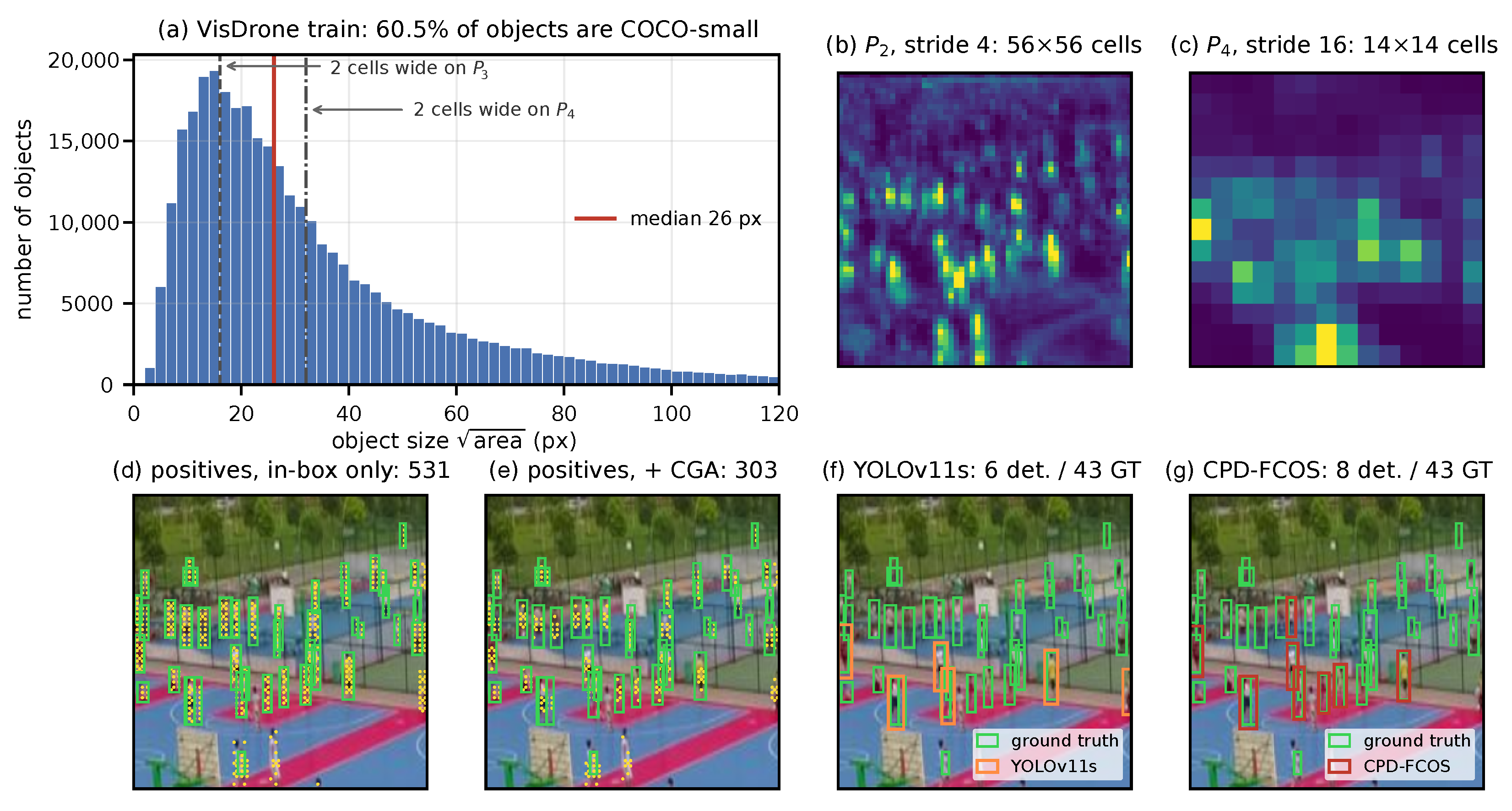
Why fine-scale representation and positive-sample quality have to be designed together. (a) Object-size distribution of the VisDrone training set. In total, of instances fall below the COCO small-object threshold, and the median object is 26 pixels across, so a typical target spans fewer than four cells at stride 8. (b,c) Responses of the trained pyramid on one crop. Individual pedestrians remain separable on the stride-4 level ( cells) but merge into a few blobs on the stride-16 level ( cells). (d,e) Positive locations selected for the same crop. The in-box rule yields 531 candidates, many of them on object borders, whereas center-constrained assignment keeps 303. (f,g) Detection outputs of YOLOv11s and CPD-FCOS at a common score threshold of . The crop was selected automatically as the densest tiny-object window in the validation image containing the largest number of tiny instances; it was not selected manually. All panels are generated from real data and trained model weights.
Figure 1.
Why fine-scale representation and positive-sample quality have to be designed together. (a) Object-size distribution of the VisDrone training set. In total, of instances fall below the COCO small-object threshold, and the median object is 26 pixels across, so a typical target spans fewer than four cells at stride 8. (b,c) Responses of the trained pyramid on one crop. Individual pedestrians remain separable on the stride-4 level ( cells) but merge into a few blobs on the stride-16 level ( cells). (d,e) Positive locations selected for the same crop. The in-box rule yields 531 candidates, many of them on object borders, whereas center-constrained assignment keeps 303. (f,g) Detection outputs of YOLOv11s and CPD-FCOS at a common score threshold of . The crop was selected automatically as the densest tiny-object window in the validation image containing the largest number of tiny instances; it was not selected manually. All panels are generated from real data and trained model weights.

Figure 2.
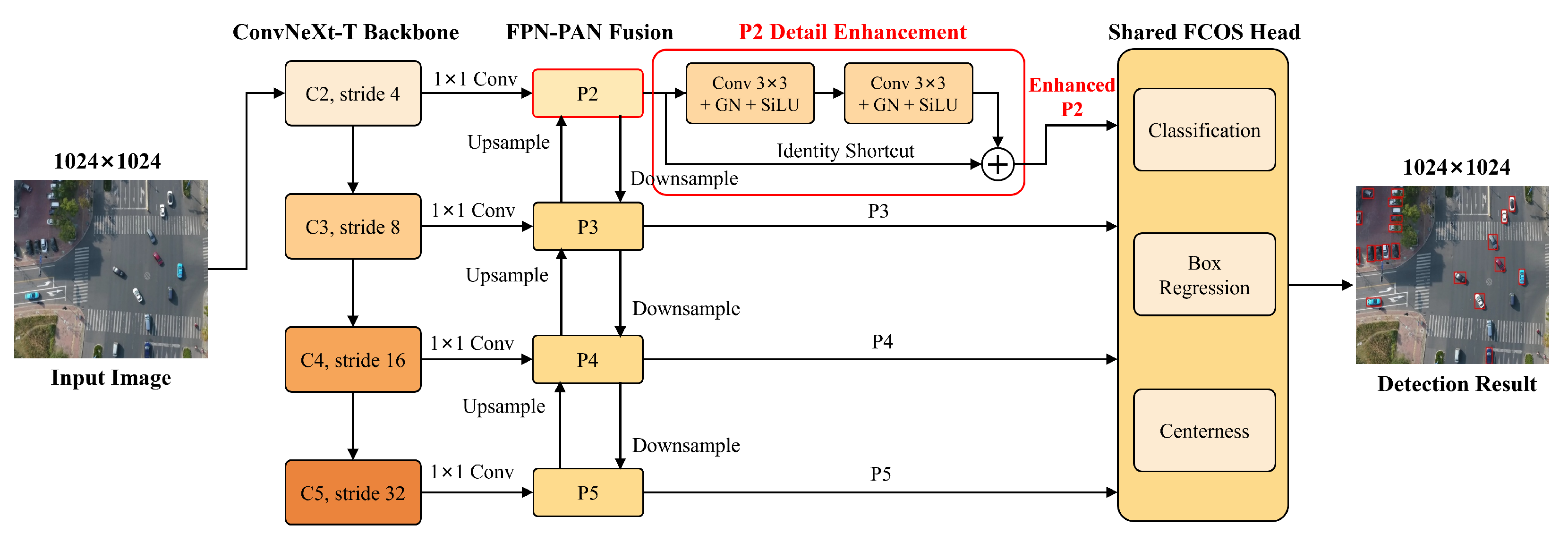
Overall architecture of the proposed CPD-FCOS. A ConvNeXt-T backbone extracts multi-scale features – at strides of 4, 8, 16, and 32. These features are projected by convolutions and fused by the FPN–PAN module through top-down upsampling and bottom-up downsampling to obtain –. The high-resolution feature is further refined by a residual detail-enhancement module composed of two Conv–GN–SiLU blocks and an identity shortcut. The enhanced and the remaining pyramid features – are then processed by a shared FCOS head for classification, box regression, and centerness prediction.
Figure 2.
Overall architecture of the proposed CPD-FCOS. A ConvNeXt-T backbone extracts multi-scale features – at strides of 4, 8, 16, and 32. These features are projected by convolutions and fused by the FPN–PAN module through top-down upsampling and bottom-up downsampling to obtain –. The high-resolution feature is further refined by a residual detail-enhancement module composed of two Conv–GN–SiLU blocks and an identity shortcut. The enhanced and the remaining pyramid features – are then processed by a shared FCOS head for classification, box regression, and centerness prediction.
Figure 3.
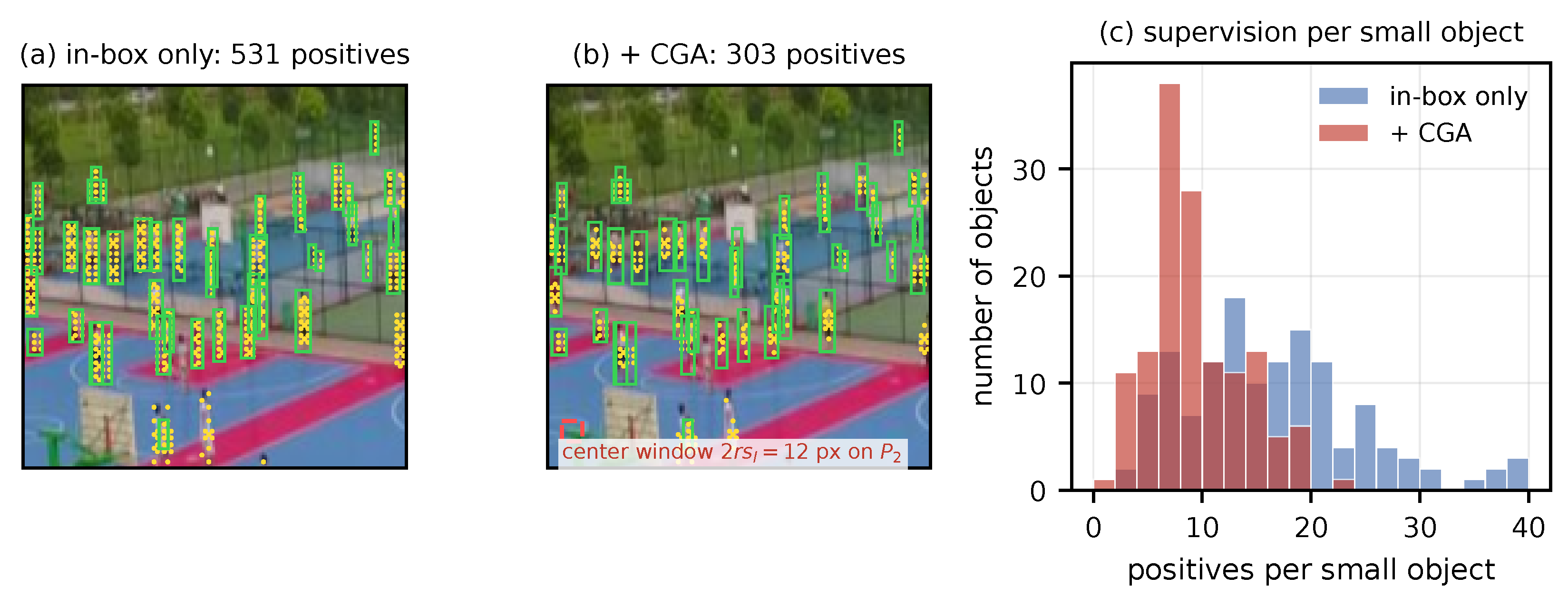
Center-constrained assignment measured on a real VisDrone crop. Green boxes denote ground-truth bounding boxes in panels (a,b). (a) With the in-box constraint alone, 531 locations become positive and many of them sit on object borders. (b) Adding the center neighborhood and the level regression range leaves 303 locations; the dashed square is the pixel center window at , drawn to scale. (c) Distribution of the number of positives assigned to each small object over 256 validation images: the in-box rule spreads to more than 40 positives per object, whereas the constrained rule concentrates the mass near the object center. Multi-object competition is resolved by minimum area.
Figure 3.
Center-constrained assignment measured on a real VisDrone crop. Green boxes denote ground-truth bounding boxes in panels (a,b). (a) With the in-box constraint alone, 531 locations become positive and many of them sit on object borders. (b) Adding the center neighborhood and the level regression range leaves 303 locations; the dashed square is the pixel center window at , drawn to scale. (c) Distribution of the number of positives assigned to each small object over 256 validation images: the in-box rule spreads to more than 40 positives per object, whereas the constrained rule concentrates the mass near the object center. Multi-object competition is resolved by minimum area.
Figure 4.
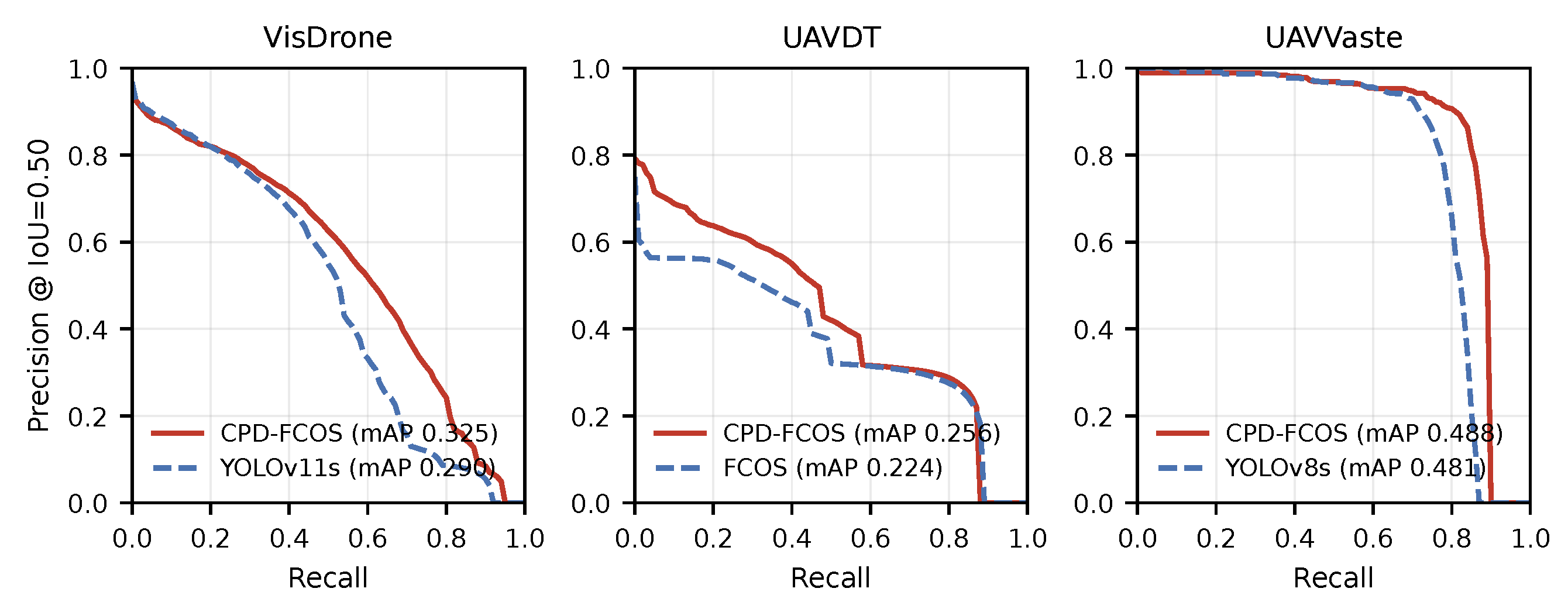
Precision–recall curves at IoU
, averaged over classes, on the complete validation split of each dataset under the original-resolution protocol. The reference detector is the highest-validation-mAP baseline for that dataset. A curve necessarily comes from one training run, whereas
Table 5 reports three-seed means; every curve here is the seed-42 run of the configuration reported in that table, and the legend gives that run’s own mAP. Checkpoint paths and SHA-256 hashes for all six curves are provided in
Supplementary File S1.
Figure 4.
Precision–recall curves at IoU
, averaged over classes, on the complete validation split of each dataset under the original-resolution protocol. The reference detector is the highest-validation-mAP baseline for that dataset. A curve necessarily comes from one training run, whereas
Table 5 reports three-seed means; every curve here is the seed-42 run of the configuration reported in that table, and the legend gives that run’s own mAP. Checkpoint paths and SHA-256 hashes for all six curves are provided in
Supplementary File S1.
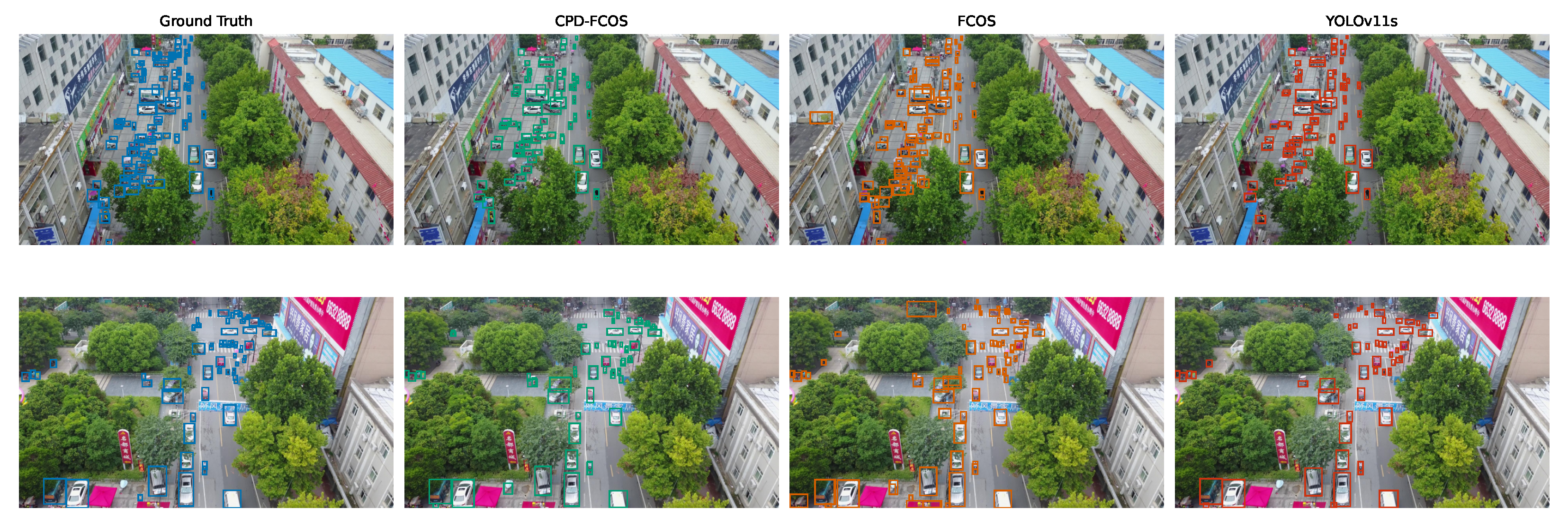
Figure 5.
Qualitative comparison on VisDrone: ground truth (GT), CPD-FCOS, FCOS, and YOLOv11s. Blue boxes denote ground truth, green boxes denote CPD-FCOS predictions, orange boxes denote FCOS predictions, and red boxes denote YOLOv11s predictions.
Figure 5.
Qualitative comparison on VisDrone: ground truth (GT), CPD-FCOS, FCOS, and YOLOv11s. Blue boxes denote ground truth, green boxes denote CPD-FCOS predictions, orange boxes denote FCOS predictions, and red boxes denote YOLOv11s predictions.
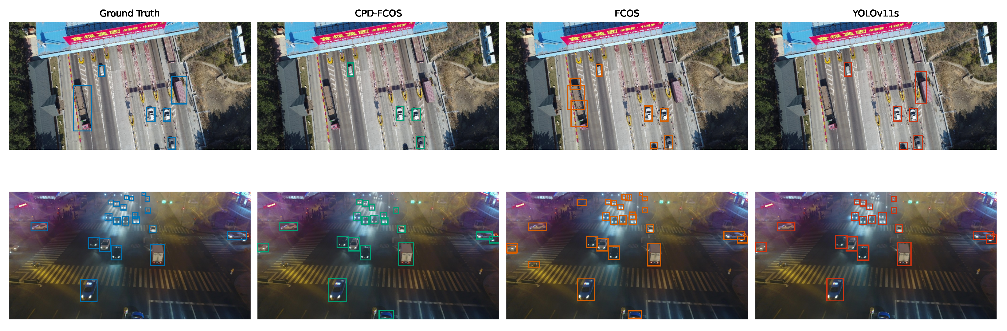
Figure 6.
Qualitative comparison on UAVDT: ground truth (GT), CPD-FCOS, FCOS, and YOLOv11s. Blue boxes denote ground truth, green boxes denote CPD-FCOS predictions, orange boxes denote FCOS predictions, and red boxes denote YOLOv11s predictions.
Figure 6.
Qualitative comparison on UAVDT: ground truth (GT), CPD-FCOS, FCOS, and YOLOv11s. Blue boxes denote ground truth, green boxes denote CPD-FCOS predictions, orange boxes denote FCOS predictions, and red boxes denote YOLOv11s predictions.
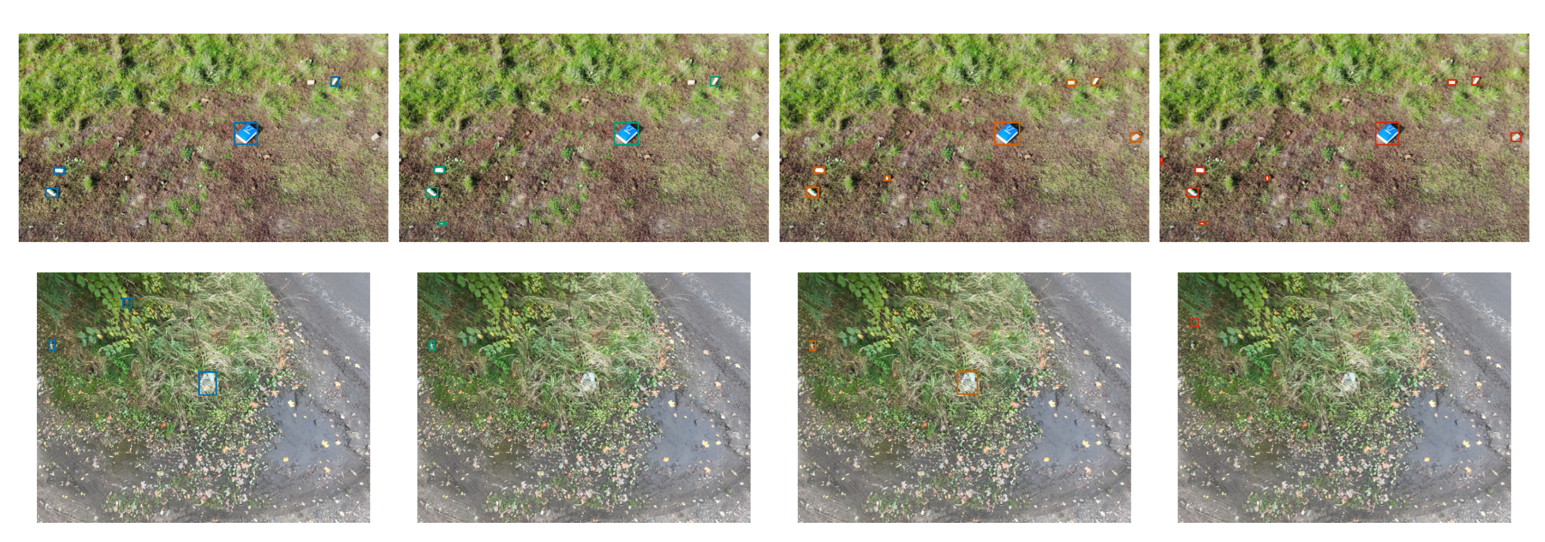
Figure 7.
Qualitative comparison on UAVVaste: ground truth (GT), CPD-FCOS, FCOS, and YOLOv11s. Blue boxes denote ground truth, green boxes denote CPD-FCOS predictions, orange boxes denote FCOS predictions, and red boxes denote YOLOv11s predictions.
Figure 7.
Qualitative comparison on UAVVaste: ground truth (GT), CPD-FCOS, FCOS, and YOLOv11s. Blue boxes denote ground truth, green boxes denote CPD-FCOS predictions, orange boxes denote FCOS predictions, and red boxes denote YOLOv11s predictions.
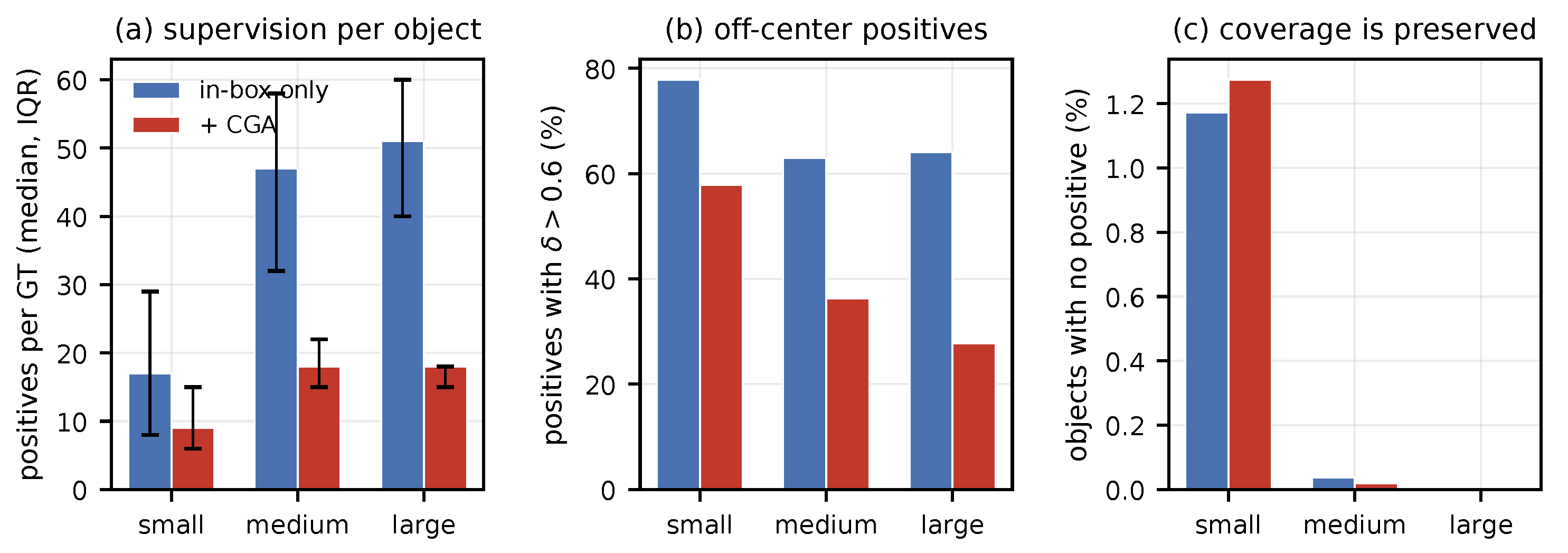
Figure 8.
Positive-sample geometry with and without center-constrained assignment, measured over 256 VisDrone validation images. (a) Median positives per object with the interquartile range. (b) Share of positives lying in the outer band of their object (). (c) Share of objects that receive no positive at all; the constrained rule preserves coverage while removing off-center supervision.
Figure 8.
Positive-sample geometry with and without center-constrained assignment, measured over 256 VisDrone validation images. (a) Median positives per object with the interquartile range. (b) Share of positives lying in the outer band of their object (). (c) Share of objects that receive no positive at all; the constrained rule preserves coverage while removing off-center supervision.
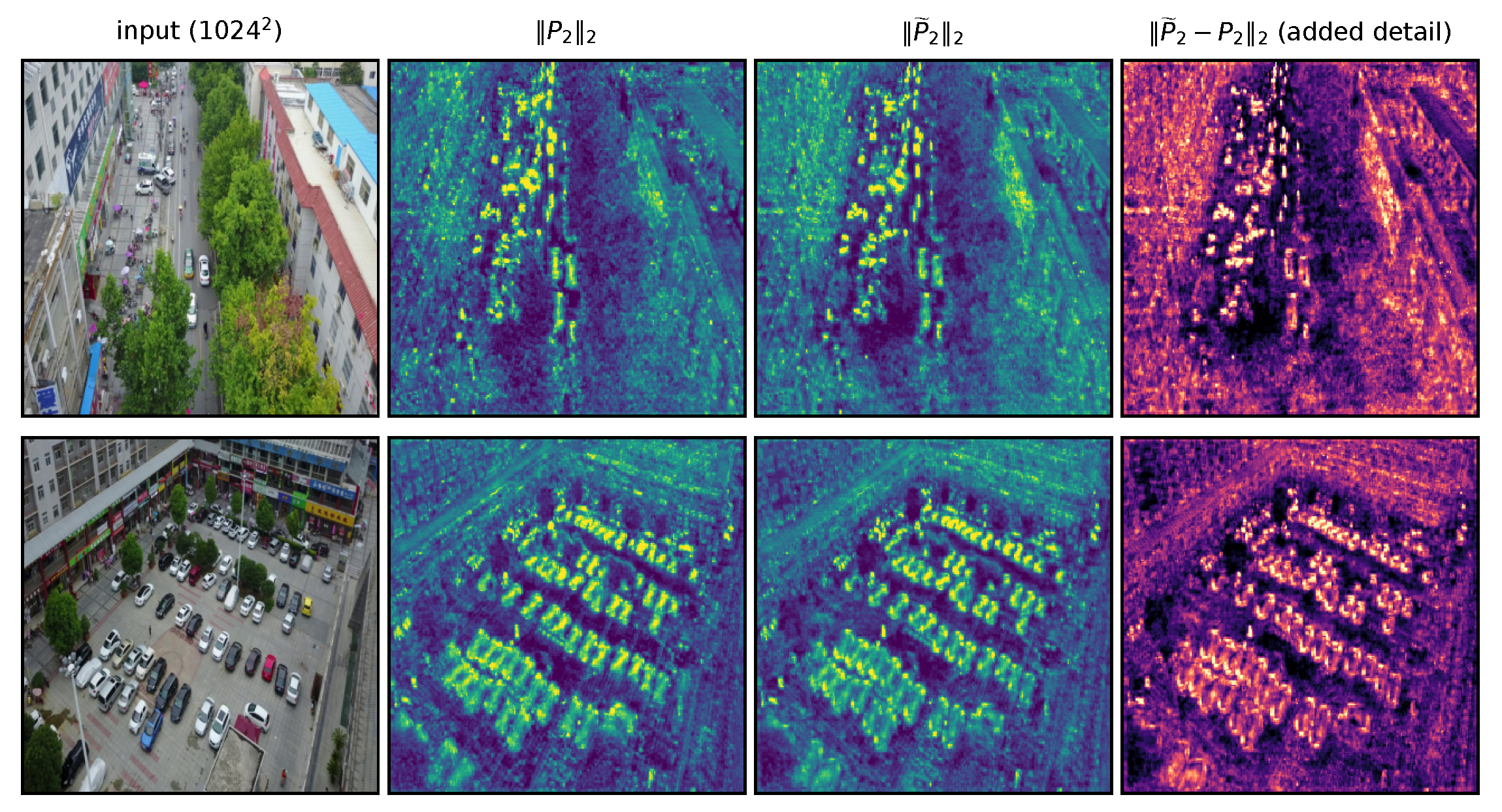
Figure 9.
The residual branch, obtained by hooking the trained module. From left: input, , , and the magnitude of the added residual. Two images are shown; the statistics quoted in the text are measured over four. The residual is comparable in magnitude to the base feature and only mildly concentrated on objects ( the background level inside ground-truth boxes).
Figure 9.
The residual branch, obtained by hooking the trained module. From left: input, , , and the magnitude of the added residual. Two images are shown; the statistics quoted in the text are measured over four. The residual is comparable in magnitude to the base feature and only mildly concentrated on objects ( the background level inside ground-truth boxes).
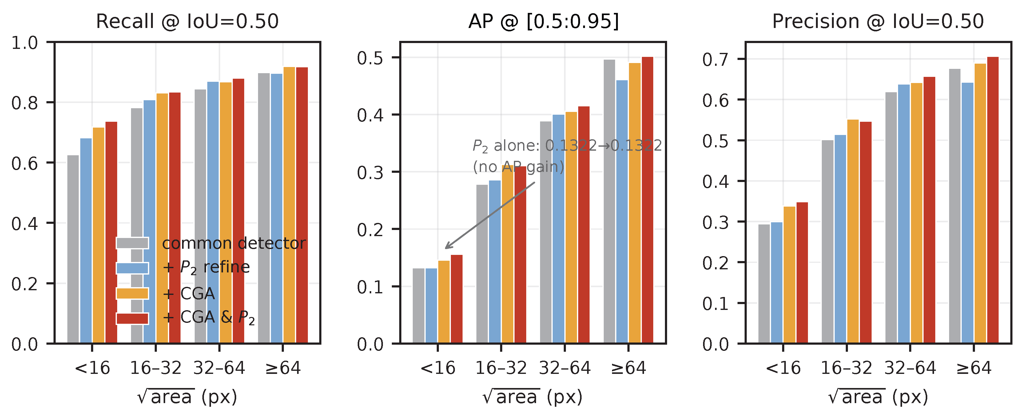
Figure 10.
Factorial variants resolved by object size on the VisDrone validation split. The
branch alone buys recall without AP in the smallest bin; constrained assignment converts the added capacity into precision. Aggregate values of these four models reproduce
Table 10 exactly.
Figure 10.
Factorial variants resolved by object size on the VisDrone validation split. The
branch alone buys recall without AP in the smallest bin; constrained assignment converts the added capacity into precision. Aggregate values of these four models reproduce
Table 10 exactly.
Table 1.
Structural distinction between standard FCOS and CPD-FCOS.
Table 1.
Structural distinction between standard FCOS and CPD-FCOS.
| Aspect | Standard FCOS | CPD-FCOS |
|---|
| Feature levels | Typically –, strides 8–128 | Real
–, strides 4–32 |
| Cross-scale fusion | Top-down FPN | Bidirectional FPN/PAN |
| Assignment | In-box candidates with center sampling and level ranges | Same
primitives, configured for – with compact overlapping ranges |
| Fine-level branch | No -specific refinement | Two-block residual
refinement only at |
| Score calibration | Classification score modulated by centerness | Unchanged from FCOS |
| Inference flow | Single forward pass | Single forward pass |
Table 2.
Statistics of the train, validation, and locked test splits.
Table 2.
Statistics of the train, validation, and locked test splits.
| Dataset | #Classes | Split | #Images | #Boxes |
|---|
| | | train | 6471 | 343,197 |
| VisDrone | 10 | val | 548 | 38,759 |
| | | test | 1610 | 75,101 |
| | | train | 6471 | 343,197 |
| VisDrone | 10 | train | 19,658 | 342,920 |
| UAVDT | 3 | val | 4485 | 79,991 |
| | | test | 16,592 | 375,884 |
| | | train | 540 | 2595 |
| UAVVaste | 1 | val | 116 | 616 |
| | | test | 116 | 507 |
Table 3.
CPD-FCOS results on the locked test splits at original resolution. Each entry is the mean ± population standard deviation over seeds 42, 123, and 456; no test run is selected as “best”.
Table 3.
CPD-FCOS results on the locked test splits at original resolution. Each entry is the mean ± population standard deviation over seeds 42, 123, and 456; no test run is selected as “best”.
| Dataset | mAP | | | | |
|---|
| VisDrone | 0.244 ± 0.001 | 0.426 ± 0.001 | 0.151 ± 0.001 | 0.342 ± 0.001 | 0.426 ± 0.018 |
| UAVDT | 0.163 ± 0.008 | 0.282 ± 0.019 | 0.117 ± 0.010 | 0.258 ± 0.010 | 0.260 ± 0.028 |
| UAVVaste | 0.528 ± 0.005 | 0.865 ± 0.012 | 0.124 ± 0.024 | 0.500 ± 0.002 | 0.640 ± 0.010 |
Table 4.
Locked-test comparison with the baseline selected by validation mAP for each dataset. Both sides are now three-seed means ± population standard deviations over seeds 42, 123 and 456. Selection was completed without test metrics.
Table 4.
Locked-test comparison with the baseline selected by validation mAP for each dataset. Both sides are now three-seed means ± population standard deviations over seeds 42, 123 and 456. Selection was completed without test metrics.
| Dataset | Method | mAP | | | | |
|---|
| VisDrone | YOLOv11s | 0.223 ± 0.001 | 0.380 ± 0.001 | 0.120 ± 0.002 | 0.336 ± 0.000 | 0.471 ± 0.008 |
| CPD-FCOS | 0.244 | 0.426 | 0.151 | 0.342 | 0.426 |
| UAVDT | FCOS | 0.167 ± 0.002 | 0.289 ± 0.003 | 0.129 ± 0.003 | 0.270 ± 0.004 | 0.126 ± 0.015 |
| CPD-FCOS | 0.163 | 0.282 | 0.117 | 0.258 | 0.260 |
| UAVVaste | YOLOv8s | 0.517 ± 0.005 | 0.817 ± 0.004 | 0.059 ± 0.009 | 0.472 ± 0.008 | 0.648 ± 0.003 |
| CPD-FCOS | 0.528 | 0.865 | 0.124 | 0.500 | 0.640 |
Table 5.
Validation-set comparison with mainstream detectors under the shared evaluation protocol (original resolution, mAP/). CPD-FCOS reports the three-seed mean; baseline entries are single runs. Every method is trained and evaluated at the same input size. The strongest baseline of each dataset was retrained with the same three seeds as CPD-FCOS and is reported as mean ± population standard deviation; the remaining entries are single runs. The last row is not part of the comparison: it retrains YOLOv8s under the full Ultralytics default to quantify what the shared 1024 setting is worth to a baseline.
Table 5.
Validation-set comparison with mainstream detectors under the shared evaluation protocol (original resolution, mAP/). CPD-FCOS reports the three-seed mean; baseline entries are single runs. Every method is trained and evaluated at the same input size. The strongest baseline of each dataset was retrained with the same three seeds as CPD-FCOS and is reported as mean ± population standard deviation; the remaining entries are single runs. The last row is not part of the comparison: it retrains YOLOv8s under the full Ultralytics default to quantify what the shared 1024 setting is worth to a baseline.
| Method | Input | VisDrone | UAVDT | UAVVaste |
|---|
| mAP | | mAP | | mAP | |
|---|
| Faster R-CNN | 1024/1707 | 0.256 | 0.181 | 0.215 | 0.188 | 0.469 | 0.145 |
| RetinaNet | 1024/1707 | 0.191 | 0.106 | 0.224 | 0.273 | 0.454 | 0.103 |
| FCOS | 1024/1707 | 0.231 | 0.148 | | | 0.456 | 0.130 |
| Faster R-CNN v2 | 1024/1707 | 0.241 | 0.164 | 0.224 | 0.190 | 0.451 | 0.124 |
| RetinaNet v2 | 1024/1707 | 0.194 | 0.105 | 0.214 | 0.197 | 0.450 | 0.106 |
| Faster R-CNN (MobileNet) | 1024/1707 | 0.149 | 0.064 | 0.180 | 0.160 | 0.336 | 0.017 |
| YOLOv8s | | 0.286 | 0.194 | 0.225 | 0.194 | | |
| YOLOv11s | | | | 0.195 | 0.173 | 0.477 | 0.209 |
| CPD-FCOS (mean) | | 0.326 | 0.251 | 0.261 | 0.287 | 0.488 | 0.196 |
| YOLOv8s (Ultralytics default) | | 0.211 | 0.112 | – | – | – | – |
Table 6.
Author-reported VisDrone2019 validation results from recent UAV-specific detectors. “NR” means that the item was not reported clearly enough for a controlled comparison. CPD-FCOS is included only as a protocol reference; cross-paper values were not reproduced in our codebase. AD-Det is reported at two backbones because its paper reports both; the ResNet-50 row is the configuration whose is available. Its inference column counts one coarse pass plus subregion passes.
Table 6.
Author-reported VisDrone2019 validation results from recent UAV-specific detectors. “NR” means that the item was not reported clearly enough for a controlled comparison. CPD-FCOS is included only as a protocol reference; cross-paper values were not reproduced in our codebase. AD-Det is reported at two backbones because its paper reports both; the ResNet-50 row is the configuration whose is available. Its inference column counts one coarse pass plus subregion passes.
| Method | Year | Input | Pretraining | Inference | AP | |
|---|
| AUHF-DETR-M [19] | 2025 | | NR | single pass | 0.309 | 0.261 |
| SARC-DETR [22] | 2026 | | COCO | single pass | 0.348 | 0.248 |
| AD-Det (ResNet-50) [20] | 2025 | | ImageNet | 1 + 4 passes | 0.353 | 0.280 |
| AD-Det (ResNeXt-101) [20] | 2025 | | ImageNet | 1 + 4 passes | 0.370 | NR |
| CPD-FCOS (3-seed mean) | 2026 | | ImageNet | single pass | 0.326 | 0.251 |
Table 7.
AD-Det reimplemented in this codebase and evaluated on the VisDrone validation split under the protocol of this paper (COCO AP, at most 100 detections per image). “Reported” values are from the original paper, whose own baseline already crops each image into four uniform parts. The reimplementation follows the published recipe (GFL, ResNet-50, , 12 epochs, SGD , decay at epochs 8 and 11, subregions, fusion NMS ); the DCC module was not reimplemented. The reimplementation is below the published figures and is reported as such; it does not license any ranking claim against AD-Det.
Table 7.
AD-Det reimplemented in this codebase and evaluated on the VisDrone validation split under the protocol of this paper (COCO AP, at most 100 detections per image). “Reported” values are from the original paper, whose own baseline already crops each image into four uniform parts. The reimplementation follows the published recipe (GFL, ResNet-50, , 12 epochs, SGD , decay at epochs 8 and 11, subregions, fusion NMS ); the DCC module was not reimplemented. The reimplementation is below the published figures and is reported as such; it does not license any ranking claim against AD-Det.
| Configuration | Passes/Image | Reported AP | Reproduced AP |
|---|
| GFL, no second stage | 1 | NR | 0.210 |
| GFL + four uniform crops (their baseline) | 1 + 4 | 0.331 | 0.293 |
| +ASOE, shared-weight fine detector | 1 + 4 | NR | 0.217 |
| +ASOE, dedicated fine detector | 1 + 4 | 0.353 | 0.278 |
| +ASOE + DCC (full AD-Det) | 1 + 4 | 0.359 | not reimplemented |
| CPD-FCOS (this paper), single pass | 1 | – | 0.326 |
Table 8.
Per-class AP on the VisDrone validation split at original resolution, against the validation-selected reference detector.
Table 8.
Per-class AP on the VisDrone validation split at original resolution, against the validation-selected reference detector.
| Method | Pedes. | People | Bicycle | Car | Van | Truck | Tricy. | Awn.-Tri. | Bus | Motor |
|---|
| YOLOv11s | 0.275 | 0.171 | 0.136 | 0.603 | 0.331 | 0.312 | 0.205 | 0.120 | 0.471 | 0.272 |
| CPD-FCOS | 0.322 | 0.221 | 0.170 | 0.631 | 0.408 | 0.340 | 0.229 | 0.121 | 0.516 | 0.296 |
Table 9.
VisDrone validation performance resolved by object size ( in pixels). Recall is measured at IoU .
Table 9.
VisDrone validation performance resolved by object size ( in pixels). Recall is measured at IoU .
| Recall (CPD-FCOS) | Recall (YOLOv11s) | AP (CPD-FCOS) | AP (YOLOv11s) |
|---|
| <16 | 0.740 | 0.367 | 0.157 | 0.097 |
| 16–32 | 0.838 | 0.660 | 0.313 | 0.255 |
| 32–64 | 0.883 | 0.801 | 0.408 | 0.406 |
| ≥64 | 0.921 | 0.851 | 0.503 | 0.514 |
Table 10.
Full-factorial ablation of center-constrained assignment (CGA) and refinement under the fixed uniform-loss recipe. A check mark indicates that the corresponding component is enabled, whereas an en dash indicates that it is disabled. Metrics are evaluated at the original image resolution.
Table 10.
Full-factorial ablation of center-constrained assignment (CGA) and refinement under the fixed uniform-loss recipe. A check mark indicates that the corresponding component is enabled, whereas an en dash indicates that it is disabled. Metrics are evaluated at the original image resolution.
| Dataset | CGA | Refine | mAP | | |
|---|
| VisDrone | – | – | 0.3010 | 0.5053 | 0.2202 |
| – | ✓ | 0.3087 | 0.5171 | 0.2275 |
| ✓ | – | 0.3225 | 0.5426 | 0.2493 |
| ✓ | ✓ | 0.3280 | 0.5483 | 0.2514 |
| UAVDT | – | – | 0.2376 | 0.4033 | 0.2346 |
| – | ✓ | 0.2545 | 0.4463 | 0.2570 |
| ✓ | – | 0.2271 | 0.3928 | 0.2685 |
| ✓ | ✓ | 0.2466 | 0.4153 | 0.3273 |
Table 11.
Direct ablation of the stride-4 level on VisDrone. Backbone, neck design, head, schedule, augmentation, seed, and evaluation protocol are identical across rows; only the pyramid depth changes. Latency is end-to-end at with batch size 1 on an idle RTX 4090 D.
Table 11.
Direct ablation of the stride-4 level on VisDrone. Backbone, neck design, head, schedule, augmentation, seed, and evaluation protocol are identical across rows; only the pyramid depth changes. Latency is end-to-end at with batch size 1 on an idle RTX 4090 D.
| Pyramid | mAP | | | Params (M) | Locations | Latency (ms) | Memory (MB) |
|---|
| – + CGA | 0.2927 | 0.4898 | 0.2003 | 38.83 | 21,504 | 22.34 | 456 |
| – + CGA | 0.3225 | 0.5426 | 0.2493 | 41.81 | 87,040 | 45.88 | 811 |
| – + CGA + refine | 0.3280 | 0.5483 | 0.2514 | 42.99 | 87,040 | 49.76 | 815 |
Table 12.
VisDrone sensitivity of depth, center radius, and regression ranges. All rows use the CGA + pathway and original-resolution evaluation.
Table 12.
VisDrone sensitivity of depth, center radius, and regression ranges. All rows use the CGA + pathway and original-resolution evaluation.
| Setting | mAP | | |
|---|
| Reference (, 2 blocks, default ranges) | 0.3280 | 0.5483 | 0.2514 |
| blocks = 1 | 0.3272 | 0.5471 | 0.2472 |
| blocks = 4 | 0.3267 | 0.5422 | 0.2439 |
| Center radius | 0.3342 | 0.5569 | 0.2531 |
| Center radius | 0.3236 | 0.5403 | 0.2441 |
| No-overlap ranges | 0.3235 | 0.5390 | 0.2452 |
| Wide overlapping ranges | 0.3308 | 0.5515 | 0.2543 |
Table 13.
Center radius under three random seeds (42, 123, 456), VisDrone validation split at original resolution, factorial recipe. Entries are mean±population standard deviation.
Table 13.
Center radius under three random seeds (42, 123, 456), VisDrone validation split at original resolution, factorial recipe. Entries are mean±population standard deviation.
| Setting | mAP | | Individual Runs (mAP) |
|---|
| | | 0.3280/0.3252/0.3229 |
| | | 0.3333/0.3327/0.3327 |
Table 14.
Does the
advantage transfer? The full main configuration is retrained at
on every dataset with three seeds and evaluated on both splits, against the reported
results of
Table 3 and
Section 4.12. Positive values favor
.
Table 14.
Does the
advantage transfer? The full main configuration is retrained at
on every dataset with three seeds and evaluated on both splits, against the reported
results of
Table 3 and
Section 4.12. Positive values favor
.
| Dataset | Split | mAP () | mAP () | mAP | |
|---|
| VisDrone | validation | 0.326 | 0.332 | | |
| UAVDT | validation | 0.261 | 0.261 | | |
| UAVVaste | validation | 0.488 | 0.488 | | |
| VisDrone | test | 0.244 | 0.248 | | |
| UAVDT | test | 0.163 | 0.156 | | |
| UAVVaste | test | 0.528 | 0.522 | | |
| Mean | | | | | |
Table 15.
UAVDT regression-range sensitivity for the CGA + pathway under original-resolution evaluation.
Table 15.
UAVDT regression-range sensitivity for the CGA + pathway under original-resolution evaluation.
| Range Setting | mAP | | |
|---|
| Default overlap | 0.2466 | 0.4153 | 0.3273 |
| No-overlap | 0.2223 | 0.3648 | 0.2540 |
| Wide overlap | 0.2512 | 0.4121 | 0.3154 |
Table 16.
Single-run pathway variants evaluated at original resolution (mAP/).
Table 16.
Single-run pathway variants evaluated at original resolution (mAP/).
| Variant | VisDrone | UAVDT | UAVVaste |
|---|
| CPD-FCOS | 0.327/0.249 | 0.272/0.288 | 0.495/0.196 |
| +soft-quality cls. | 0.311/0.228 | 0.258/0.295 | 0.491/0.187 |
| +SA-WIoU loc. | 0.328/0.251 | 0.236/0.242 | 0.486/0.173 |
Table 17.
Independent ablation of scale-aware loss reweighting, three-seed mean ± std (original resolution, complete validation split, torchmetrics). “Ours” is the final model (uniform positive-sample weights); “+reweighting” adds scale-aware weights on top of it.
Table 17.
Independent ablation of scale-aware loss reweighting, three-seed mean ± std (original resolution, complete validation split, torchmetrics). “Ours” is the final model (uniform positive-sample weights); “+reweighting” adds scale-aware weights on top of it.
| Dataset | Config | mAP | |
|---|
| VisDrone | Ours | | |
| +reweighting | | |
| UAVDT | Ours | | |
| +reweighting | | |
| UAVVaste | Ours | | |
| +reweighting | | |
Table 18.
Efficiency comparison (single input, batch size 1, RTX 4090 D). GFLOPs are framework-specific profiler estimates and exclude dynamic detection post-processing. Latency is implementation-specific and is not a controlled cross-framework or end-to-end onboard comparison. Each model is measured after clearing previously resident models from GPU memory.
Table 18.
Efficiency comparison (single input, batch size 1, RTX 4090 D). GFLOPs are framework-specific profiler estimates and exclude dynamic detection post-processing. Latency is implementation-specific and is not a controlled cross-framework or end-to-end onboard comparison. Each model is measured after clearing previously resident models from GPU memory.
| Method | Params (M) | GFLOPs | Latency (ms) | FPS | Memory (MB) |
|---|
| Faster R-CNN | 41.3 | 210.6 | 19.8 | 50.4 | 657 |
| RetinaNet | 32.4 | 211.8 | 17.6 | 56.9 | 430 |
| FCOS | 32.1 | 206.1 | 18.4 | 54.3 | 429 |
| YOLOv8s | 11.2 | 73.8 | 4.2 | 237.8 | 216 |
| YOLOv11s | 9.5 | 55.6 | 6.0 | 166.2 | 235 |
| CPD-FCOS (Ours) | 43.0 | 766.6 | 46.4 | 21.5 | 724 |
Table 19.
End-to-end latency by stage (single
image, batch size 1, idle RTX 4090 D, median over 50 real validation images). The
–
column is the pyramid ablation of
Table 11.
Table 19.
End-to-end latency by stage (single
image, batch size 1, idle RTX 4090 D, median over 50 real validation images). The
–
column is the pyramid ablation of
Table 11.
| Stage | CPD-FCOS (ms) | – (ms) | Ratio |
|---|
| Preprocessing | 2.28 | 2.02 | 1.13× |
| Backbone + neck | 22.73 | 12.24 | 1.86× |
| Detection head | 21.53 | 6.15 | 3.50× |
| Decoding + NMS | 2.93 | 1.76 | 1.67× |
| Remap to original resolution | 0.16 | 0.11 | 1.45× |
| End-to-end | 49.76 (20.1 FPS) | 22.34 (44.8 FPS) | 2.23× |




 ,
,