Fine-Grained Tree Species Classification in Urban Forests via Phenology–Structure Synergistic Fusion of Multi-Source Remote Sensing Data

Highlights

What are the main findings?

• HybridFusion achieved 90.44% overall accuracy and 85.06% tree species accuracy by integrating high-resolution imagery, multi-temporal NDVI, LiDAR, and hyperspectral–semantic priors.
• Phenological and structural features raised Tree OA from 67.29% to 81.90%, and reliability-aware hyperspectral fusion further increased it to 85.06%.

What are the implications of the main finding?

• Integrating complementary spatial, phenological, structural, and spectral–semantic information reduces tree species confusion and enables adaptive fusion to overcome scale and representation differences among remote sensing sources more effectively than simple input-level stacking.
• The resulting fine-scale, park-wide tree species maps provide spatially explicit information on species composition and distribution, supporting urban forest inventories, targeted maintenance, biodiversity assessment, ecosystem-service evaluation, and forest-health monitoring.

Abstract

Urban forest tree species composition and spatial distribution are essential for refined greenspace management, ecosystem-service assessment, and forest-health monitoring. High-resolution imagery captures crown texture and spatial boundaries, multi-temporal NDVI reflects phenological differences, LiDAR provides canopy height and structural information, and hyperspectral imagery offers detailed spectral discrimination. However, differences in spatial resolution and information representation limit the effectiveness of simple feature stacking. Motivated by the challenges associated with heterogeneous stand structure, similarity among broadleaved species, and insufficient multi-source fusion, this study developed HybridFusion for fine-grained tree species classification in the northern section of Beijing Olympic Forest Park. The model uses 0.5 m high-resolution imagery as its spatial basis and integrates NDVI phenological features from March, April, and August, LiDAR-derived canopy structural features, and hyperspectral–semantic priors through branch encoding, dynamic gated fusion, and reliability-aware hyperspectral modulation. The full-modality model achieved optimal performance (OA: 90.44%; Tree OA: 85.06%; mIoU: 77.88%). Poplar achieved an F1 score of 95.31%, while willow, coniferous trees, and other tree species reached 86.27%, 84.90%, and 85.35%, respectively. Ablation studies confirmed the complementary value of the multi-source data: integrating NDVI and LiDAR increased Tree OA from 67.29% to 81.90%, and the addition of hyperspectral–semantic priors further raised it to 85.06%. These results demonstrate the effectiveness of jointly exploiting phenological, structural, and spectral–semantic information for fine-scale urban forest inventory and management.

1. Introduction

Urban forest parks are important spatial systems that connect ecological processes with public needs in built environments. Through canopy shading, evapotranspiration, pollutant deposition, and carbon storage, their vegetation contributes to the regulation of urban heat, water, carbon, and pollution cycles and affects environmental quality and human health [1,2,3,4,5,6]. Tree species composition and spatial arrangement are fundamental descriptors of structural and functional heterogeneity in urban forests and provide a basis for ecosystem-service assessment, biodiversity conservation, stand-health monitoring, and pest and disease risk management [7]. Compared with natural forests, urban forests commonly exhibit complex species composition, intensive anthropogenic disturbance, interlaced crowns, and diverse background land covers. Rapid and accurate acquisition of tree species information is therefore a foundational technical requirement for urban forest inventories and refined management [8,9,10].

Conventional tree species surveys primarily rely on plot establishment, individual-tree measurements, and visual interpretation. Although these approaches can provide accurate local species information, their application to large-area and repeated monitoring is constrained by high labor costs and limited updating efficiency. Remote sensing has therefore become an important approach for tree species identification and distribution mapping because of its spatial continuity, repeatability, and multiscale representation [11,12]. Early studies commonly used medium- and low-spatial-resolution data, such as MODIS and Landsat, to identify forest types or dominant species groups. Although these data are suitable for regional monitoring, mixed pixels limit crown-boundary delineation and fine-scale species separation in mixed stands [13]. Multi-temporal imagery records spectral responses during green-up, leaf expansion, peak growth, and senescence, providing temporal cues for distinguishing species with similar appearances but different phenological rhythms [14]. High-spatial-resolution data from WorldView, Pleiades, GF-2, and unmanned aerial vehicles can represent crown outlines, texture, and local spatial organization more clearly, extending tree species classification from the stand scale to patch- and individual-tree-scale applications [15,16,17]. Nevertheless, a single optical image mainly captures the spectral and spatial properties of the crown surface and remains limited for species with similar crown forms or spectral responses, particularly under shadow occlusion. Consequently, LiDAR-derived canopy height and three-dimensional structure, continuous hyperspectral responses, and phenological differences from multi-temporal imagery have been increasingly incorporated to provide complementary observations of tree species [18,19,20,21,22].

Early remote sensing-based tree species classification methods typically extracted spectral, textural, vegetation-index, geometric, and topographic features from imagery, combined them with LiDAR height, intensity, and canopy structural features, and then used classifiers such as support vector machines, random forests, and XGBoost to establish nonlinear relationships between features and species classes [23,24]. These methods can operate with relatively small sample sets and organize diverse statistical features effectively. However, their performance depends strongly on manual feature design, scale selection, and feature combination strategies [25]. When data sources differ substantially in spatial resolution, numerical distribution, and semantic level, input-level stacking or static feature concatenation cannot adequately characterize the class- and location-dependent contributions of different observations. Such strategies may also introduce registration errors and observation noise into a common feature space [26,27]. These limitations highlight the need for representation learning methods that can preserve the characteristics of each data source while modeling their complementary relationships [16,28,29].

Deep learning offers a technical pathway for hierarchical representation learning and end-to-end modeling of tree species characteristics. Convolutional neural networks can progressively extract edges, textures, crown morphology, and high-level semantic features from high-resolution imagery and have been applied to individual-tree species classification and vegetation semantic segmentation [29,30,31]. For hyperspectral data with high dimensionality and strong inter-band correlation, models such as 3D-CNNs enhance class representation by jointly learning spatial–spectral features [21,32]. Multi-modal deep learning has further introduced branch-specific encoding, intermediate-layer interaction, attention modulation, and cross-modal relationship modeling to learn interactions among heterogeneous observations. However, the effectiveness of these approaches depends on how differences in spatial support, semantic level, and information reliability are reconciled [18,33,34]. In fine-scale urban forest classification, sub-meter optical imagery and coarser hyperspectral and LiDAR grids describe the scene at different spatial supports, while the discriminative value of each modality varies across tree species and local environments [35,36]. Crown overlap, shadow occlusion, and the visual similarity of closely related broadleaf species further increase uncertainty near class boundaries. The resulting challenge is to learn spatially precise representations while aligning cross-modal features, adaptively weighting modality contributions according to spatial and semantic context, and limiting the influence of unreliable auxiliary information [22,37,38].

The high cost of field surveys and crown-level annotation has also motivated increasing interest in label-efficient learning. Recent studies have explored several complementary strategies. Weakly supervised methods can exploit accessible low-resolution historical land-cover maps as inexact guidance; for example, Li et al. developed Paraformer with a pseudo-label-assisted training module to refine spatially mismatched coarse labels for high-resolution land-cover mapping [39]. Semi-supervised remote sensing segmentation combines limited labeled samples with abundant unlabeled imagery, while decoupled learning and confidence-ranking weights reduce the influence of erroneous and class-imbalanced pseudo-labels [40]. Difference-complementary learning and label reassignment further improve pseudo-label utilization in multi-modal optical-SAR segmentation [41]. Under extremely limited supervision, Confucius tri-learning jointly trains two classifiers and one generator, enabling the classifiers to exchange reliable “good” quasi-labels and reject generated “bad” examples [42]. Subsequent theoretical analysis connected mutual-guide learning with Confucius tri-learning and provided a theoretical justification for this mutual-guidance process under limited supervision [43]. However, even when pseudo-labels provide additional supervisory information, reliable fine-grained tree species mapping requires the labels to remain consistent with crown boundaries and the associated spatial, phenological, structural, and spectral representations to be properly aligned. This requirement motivates the present study, which uses field surveys and visual interpretation to construct reference labels, takes high-resolution imagery as the spatial basis, and integrates multi-temporal NDVI, LiDAR canopy structural features, and hyperspectral–semantic priors through branch-specific encoding, dynamic gated fusion, and reliability-aware semantic modulation.

This study focuses on the northern section of Olympic Forest Park, Beijing. High-resolution imagery was used as the spatial information source and was integrated with NDVI phenological features, LiDAR canopy structural features, and hyperspectral–semantic priors. Field surveys and visual interpretation were combined to construct the tree species classification sample set. To address differences in information form and reliability across data sources, we developed a phenology–structure synergistic HybridFusion model: (1) the high-resolution branch uses branch encoding and dynamic gating to regulate the contributions of spatial, phenological, and structural features through pixel- and channel-level weights; and (2) the hyperspectral branch introduces a reliability-aware semantic prior that allows coarse-resolution spectral information to contribute to fine-grained species discrimination in a controlled manner. A set of comparative experiments evaluates how each information source and its interaction mechanisms affect classification accuracy, class confusion, and spatial mapping stability, providing a methodological reference for urban forest species mapping and coordinated use of multi-source remote sensing data.

2. Study Area and Multi-Source Remote Sensing Data

2.1. Study Area

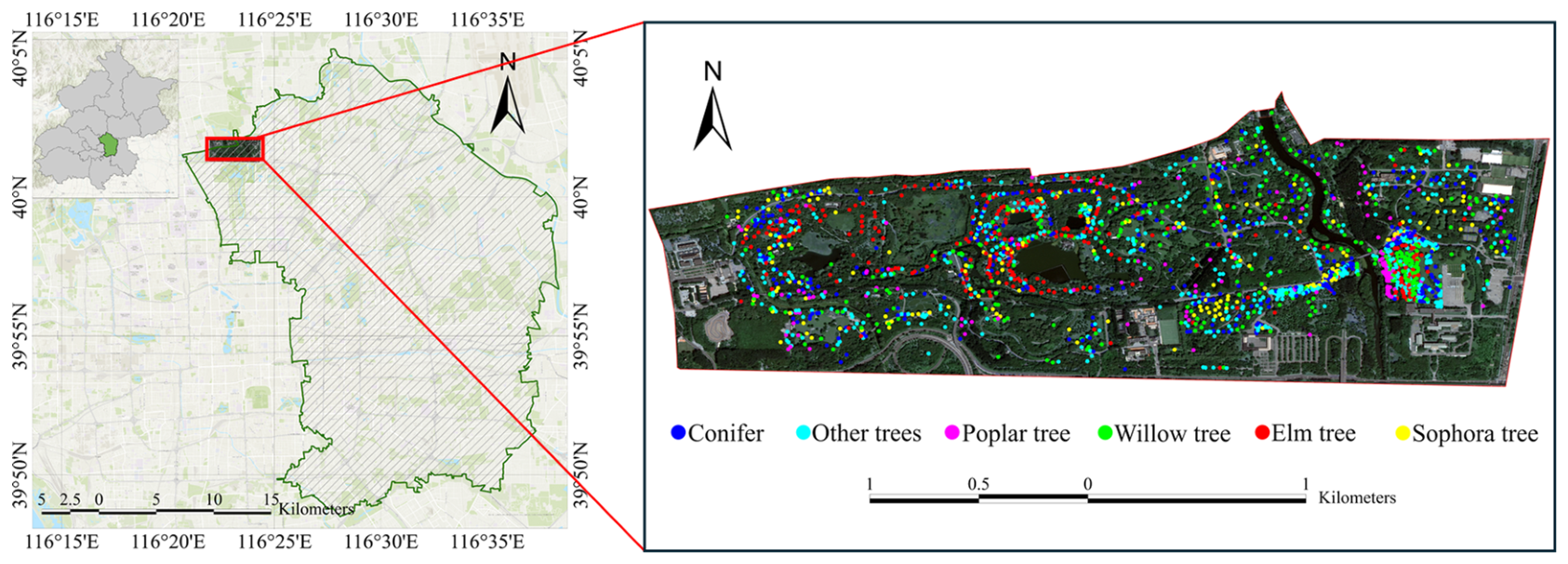
This study was conducted in the North Area of Beijing Olympic Forest Park (Figure 1), an approximately 3.0 km² urban planted forest ecosystem located on Beijing’s central axis. Shaped by long-term artificial tending and natural succession, the moderately undulating terrain supports a complex stand structure comprising coniferous, deciduous broadleaved, and mixed forests. The field inventory recorded 25 tree taxa, whose common names, scientific names, broad vegetation categories, and assignments to the model classes are summarized in

Table 1. Common and scientific names of the tree taxa recorded in the study.

Common Name	Scientific Name	Model Class
Chinese pine	Pinus tabuliformis	Conifer
Deodar cedar	Cedrus deodara	Conifer
Chinese arborvitae	Platycladus orientalis	Conifer
Chinese willow	Salix matsudana	Willow
Weeping willow	Salix babylonica	Willow
Siberian elm	Ulmus pumila	Elm
Chinese elm	Ulmus parvifolia	Elm
White poplar	Populus alba	Poplar
Canadian poplar	Populus × canadensis	Poplar
Black locust	Robinia pseudoacacia	Sophora
Japanese pagoda tree	Styphnolobium japonicum	Sophora
Green ash	Fraxinus pennsylvanica	Other trees
Mexican ash	Fraxinus uhdei	Other trees
Apricot	Prunus armeniaca	Other trees
Flowering almond	Prunus triloba	Other trees
Shantung maple	Acer truncatum	Other trees
Crabapple	Malus spp.	Other trees
Ginkgo	Ginkgo biloba	Other trees
Chinese wingnut	Pterocarya stenoptera	Other trees
Linden	Tilia spp.	Other trees
Goldenrain tree	Koelreuteria paniculata	Other trees
Persimmon	Diospyros kaki	Other trees
Oak	Quercus spp.	Other trees
Mulberry	Morus spp.	Other trees
Paper mulberry	Broussonetia papyrifera	Other trees

. Representative taxa include Chinese pine (Pinus tabuliformis), deodar cedar (Cedrus deodara), Chinese arborvitae (Platycladus orientalis), Chinese willow (Salix matsudana), weeping willow (Salix babylonica), Siberian elm (Ulmus pumila), Japanese pagoda tree (Styphnolobium japonicum), green ash (Fraxinus pennsylvanica), Shantung maple (Acer truncatum), and white poplar (Populus alba). Table 1 complements Figure 1 by clarifying both the taxonomic composition of the study area and the aggregation of the recorded taxa into the model classes. Spatially, the landscape is highly heterogeneous. Contiguous pure stands resulting from planned planting coexist with succession-driven mixed patches characterized by overlapping crowns and intermixed species. Furthermore, artificial features such as roads, water bodies, and buildings are interspersed throughout the forested landscape. This high degree of structural and landscape complexity provides an appropriate test site for evaluating fine-scale tree species identification using multi-source remote sensing data across pure stands, mixed stands, and forest–non-forest transition zones.

2.2. Multi-Source Remote Sensing Data

2.2.1. Multispectral Data

The primary dataset comprised multi-temporal Beijing-3 satellite imagery (2024–2025). Following radiometric calibration, atmospheric correction, orthorectification, and pan-sharpening, 0.5 m resolution multispectral images were generated to capture crown boundaries and textural details. Additionally, optical aerial imagery covering the North Area of Beijing Olympic Forest Park was acquired by an unmanned aerial vehicle (UAV) in 2025 at a spatial resolution of 0.1 m. This imagery was used solely as auxiliary data for visual interpretation, sample identification, and label verification.

2.2.2. Hyperspectral Data

Hyperspectral data were acquired in August 2024 using the GF-5B Advanced Hyperspectral Imager (AHSI). The imagery has a native spatial resolution of approximately 30 m and contains 330 contiguous bands covering 400–2500 nm, with a spectral resolution of 5–10 nm. Atmospheric correction was performed using the Fast Line-of-sight Atmospheric Analysis of Spectral Hypercubes (FLAASH), which is based on the MODTRAN radiative-transfer model, to obtain surface reflectance. The hyperspectral data were georeferenced to the common map reference and extracted over the same geographic bounds as each classification patch. For network processing, each hyperspectral window was represented as a 330 × 5 × 5 input patch. Because of its coarse native resolution, the hyperspectral imagery was not used for individual crown-boundary delineation; instead, it was used to generate a patch-level spectral–semantic prior for species classification.

2.2.3. LiDAR Data

Forest three-dimensional structural data were derived from airborne LiDAR point clouds acquired in 2022 using a Leica CityMapper-2 system mounted on a piloted P-750 aircraft. The flight altitude was 2100 m, the pulse repetition frequency was 2000 Hz, the average point density was approximately 16 points m⁻², and up to five returns were recorded per pulse. The flight was conducted under clear-sky conditions. The point clouds were processed in LiDAR360 through strip adjustment, noise removal, classification, and visual inspection. Ground, vegetation, building, vehicle, and other points were identified. A digital elevation model was generated from ground points, and vegetation-point heights were normalized relative to the ground surface. The normalized vegetation points were aggregated into 2 m × 2 m grid cells, where maximum height, P95 height, mean height, height standard deviation, height coefficient of variation, canopy relief ratio, canopy closure, gap fraction, and leaf area index were calculated. The resulting structural rasters were transformed to the common coordinate reference system. For each label patch, the corresponding geographic extent was extracted, aligned with the 2 m classification grid, and resampled to the spatial dimensions required by the model.

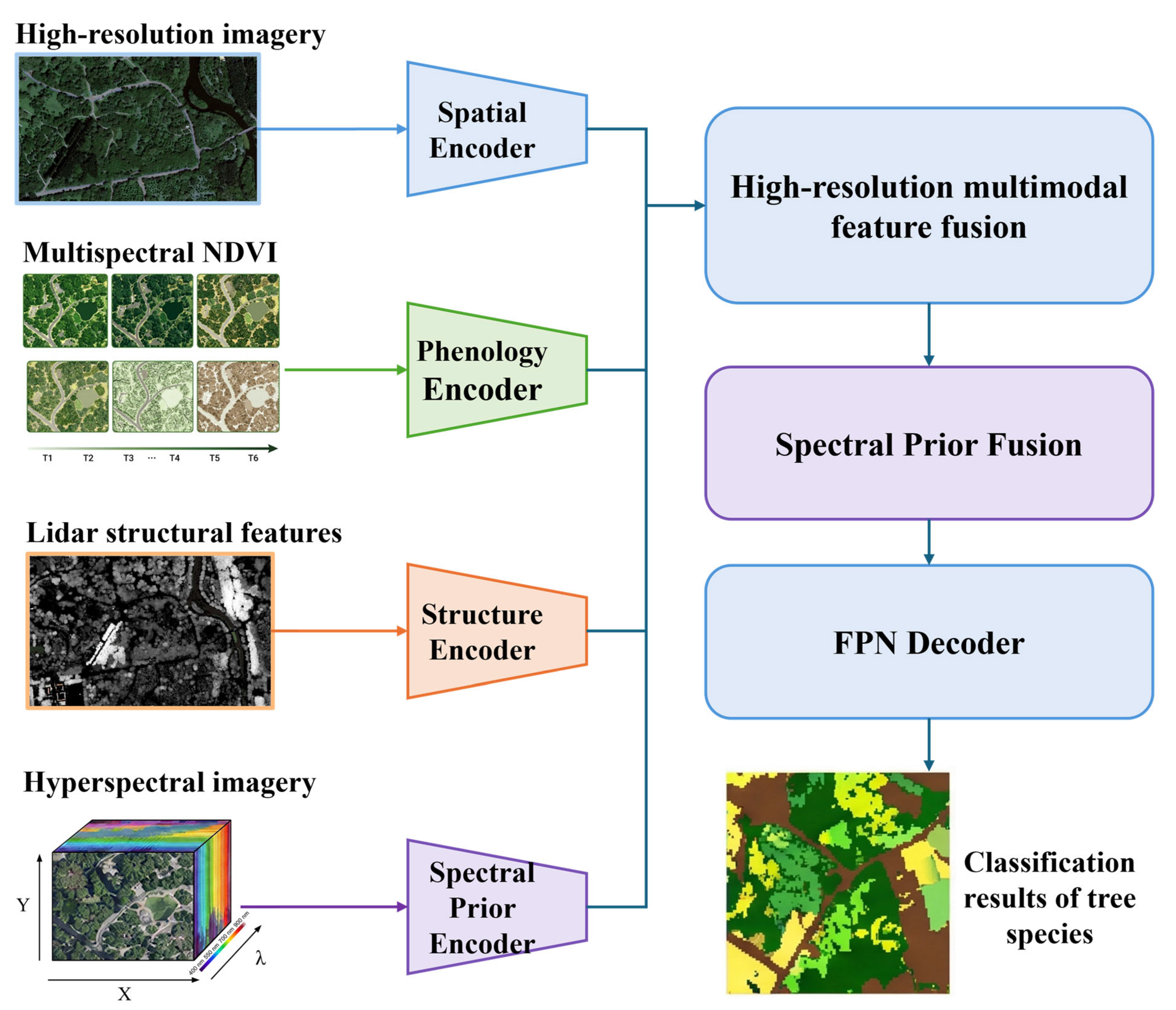
The relationships among the multi-source remote sensing data, the derived features, and their roles in the tree species classification framework are summarized in Figure 2. High-resolution imagery provides spatial and textural information, multi-temporal NDVI represents phenological variation, LiDAR provides canopy structural features, and hyperspectral imagery supplies spectral–semantic priors. These complementary data sources are subsequently integrated by the HybridFusion model for fine-grained tree species classification.

2.3. Ground Survey Data

Field surveys of tree species were conducted in the northern section of Olympic Forest Park, Beijing, in autumn 2025. According to the area’s species composition, stand types, and spatial distribution, sample locations covered typical settings, including extensive pure stands, mixed stands of Conifer and broadleaf species, forest edges, roadside green belts, forests surrounding water bodies, and landscape planting areas, thereby improving coverage across stand structures and background conditions. During field surveys, high-precision GPS equipment was used to record sample coordinates, tree species names, class attributes, and surrounding environmental information. Photographs of trunks, bark, leaves, branches, canopy morphology, and the local environment were also collected.

Areas with conspicuous crown interlacing or trees whose species could not be confirmed directly in the field were rechecked using field observations, 0.1 m aerial imagery, individual-tree detail photographs, and information from nearby samples to reduce the effects of crown mismatches and species misidentification on subsequent label production. The compiled survey comprised 1960 field tree species samples, covering the principal species in the study area, including Willow, Elm, Sophora, Poplar, and various conifers. Together with aerial image-assisted interpretation, these samples were used to prepare and validate the tree species labels.

2.4. Sample Production and Dataset Partitioning

This study conducted tree species sample interpretation and label production based on field survey points, field photographs, 0.1 m ultra-high-resolution aerial imagery, and 0.5 m high-resolution remote sensing imagery. After overlaying the field survey points onto the high-resolution imagery, polygon labels were created for areas with clearly identified tree species attributes and relatively clear canopy boundaries, using information such as tree crown boundaries, canopy texture, spatial location, and field photographs. Areas with severe crown overlap, obvious shadow occlusion, or unreliable tree species identification were excluded from the main training samples to reduce the influence of label uncertainty on model learning. Considering the complex tree species composition of the North Area of Beijing Olympic Forest Park and the limited sample size of some classes, this study did not establish a separate class for every original tree species. Instead, a classification system was constructed by considering sample size, ecological dominance, and remote sensing separability. Willow tree, elm tree, sophora tree, and poplar tree were treated as separate classes because they are major dominant broadleaf species in the study area. Chinese pine and Chinese arborvitae were merged into the “conifer” class. Species with fewer samples or scattered spatial distributions, such as ash, ginkgo, trident maple, paper mulberry, London plane, purple-leaf plum, apricot, and flowering crabapple, were merged into the “other tree species” class. Roads, water bodies, grassland, bare land, buildings, shadows, and similar areas were assigned to the “non-tree” class. This produced a seven-class classification system: Non-tree, Willow tree, Conifer, Elm tree, Sophora tree, Poplar tree, and Other tree species.

Label production was based on manually delineated tree crown polygons. To reconcile the spatial-resolution differences among the multi-source datasets, the original labels and the 0.5 m high-resolution imagery were transformed to a common 2 m classification grid. Subsequent model training, accuracy assessment, and full-area tree species mapping were conducted at this 2 m spatial resolution. Each label patch contains 20 × 20 cells and covers a geographic extent of 40 m × 40 m. The high-resolution imagery, NDVI features, and LiDAR structural features were extracted over this extent as 80 × 80 arrays, whereas the hyperspectral data were extracted over the same geographic extent and represented as a 330 × 5 × 5 coarse input patch. Thus, the hyperspectral input provides patch-level spectral–semantic context rather than one-to-one information for each 2 m label cell. During preprocessing, all source windows were generated through CRS-aware reprojection to the label-grid bounds. Patches with no source-label overlap were rejected. The study area contained 1960 field tree species samples, 889 tree species label polygons, and 26,381 valid tree species label pixels. A training set and validation set were then constructed, including 676 training samples and 64 validation samples, for a total of 740 patch samples used for model training, parameter selection, and classification accuracy assessment. The classification system and sample quantities are shown in

Table 2. Tree species sample and label counts.

ID	Class	Sample Count	Sample Proportion	Number of Label Polygons	Label Polygon Proportion	Number of Labeled Pixels	Labeled Pixel Proportion
0	Non-tree	-	-	Background supplementation	-	Background supplementation	-
1	Willow	346	0.18	116	0.13	4112	0.16
2	Conifer	400	0.20	189	0.21	1861	0.07
3	Elm	306	0.16	119	0.13	3214	0.12
4	Sophora	191	0.10	99	0.11	4634	0.18
5	Poplar	136	0.07	46	0.05	8298	0.31
6	Other trees	581	0.30	320	0.36	4262	0.16
Total	Total tree species classes	1960	-	889	-	26,381	-

.

3. Methodology

3.1. Overall Workflow

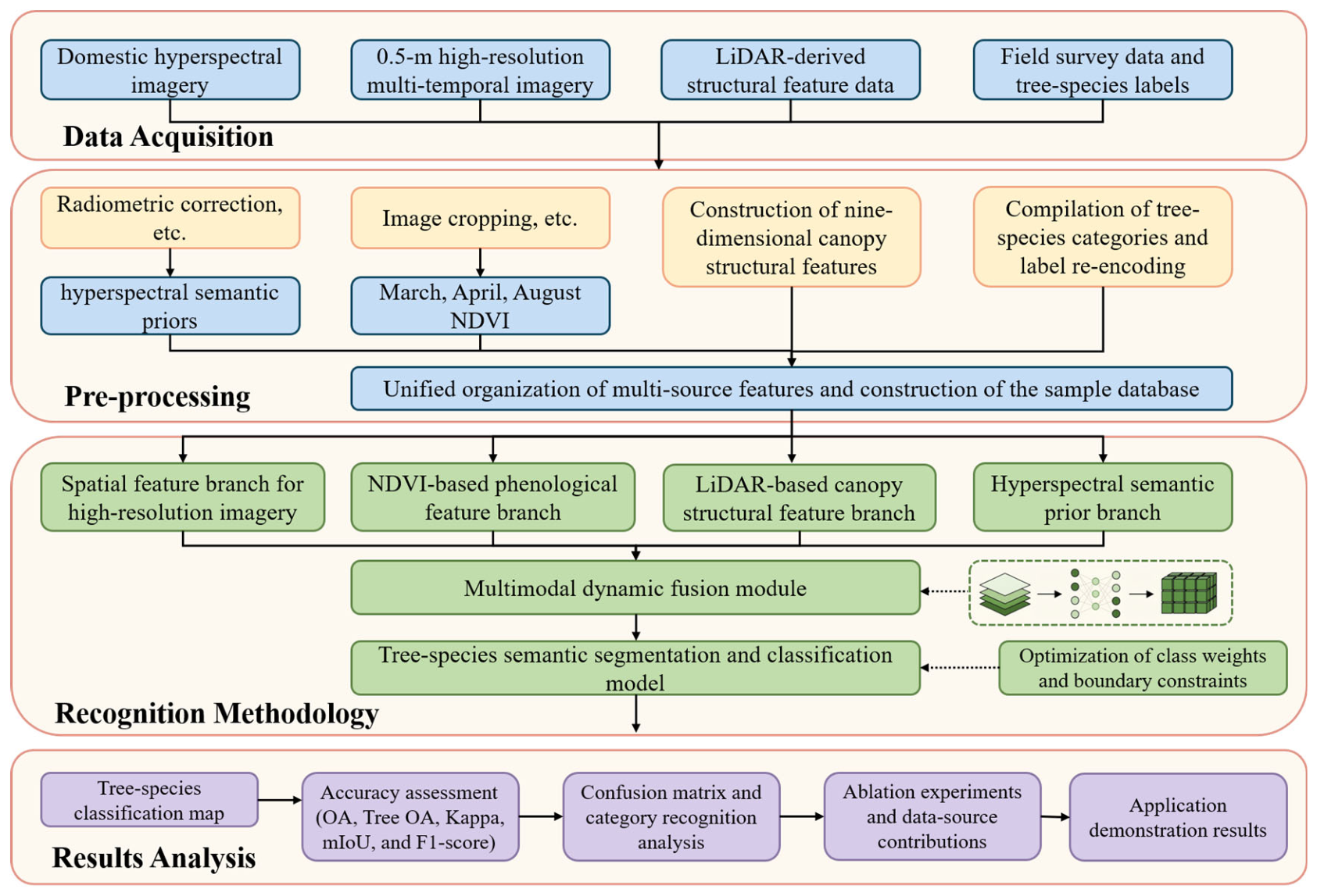
We developed a synergistic multi-source remote sensing fusion framework for fine-grained urban forest tree species classification (Figure 3). The framework uses multi-temporal high-resolution imagery as the primary source of spatial information and integrates LiDAR canopy structural features, hyperspectral–semantic priors, and field survey labels within a common spatial reference for sample organization, model training, classification mapping, and accuracy assessment. A 2 m classification grid is used as the fundamental unit for coordinated representation of the multi-source data. Crown spatial texture, phenological variation, vertical structure, and spectral–semantic information are incorporated into a unified classification workflow to improve the stability of tree species recognition in complex urban forest settings.

High-resolution imagery represents crown boundaries, texture, and local spatial morphology. NDVI and temporal-difference features derived from March, April, and August imagery describe phenological differences before and during the growing season. Height-normalized and gridded LiDAR point clouds provide nine-dimensional canopy structural features. Hyperspectral imagery supplies a spectral–semantic prior that complements subtle interspecies spectral differences. Together with manually annotated labels, these features form the sample library and are fed into HybridFusion for pixel-level tree species classification. Performance is evaluated using overall accuracy, the Kappa coefficient, mIoU, Macro-F1, confusion matrices, and ablation experiments to quantify the contributions of individual data sources and fusion strategies.

3.2. Hybridfusion Architecture

HybridFusion is the multi-source remote sensing model developed in this study for tree species classification. Formulated as a semantic segmentation task, the model takes high-resolution imagery, multi-temporal NDVI, LiDAR structural features, and hyperspectral–semantic priors as inputs. Branch encoding, dynamic fusion, semantic modulation, and classification decoding produce predictions for seven classes: Non-tree, Willow, Conifer, Elm, Sophora, Poplar, and Other trees. The design explicitly exploits complementary information across modalities: high-resolution imagery provides crown-level spatial detail; NDVI captures phenological variation; LiDAR characterizes three-dimensional canopy structure; and the hyperspectral prior contributes spectral–semantic information. Their integration improves tree species discrimination in complex backgrounds [44].

3.2.1. Multi-Modal Feature Encoding

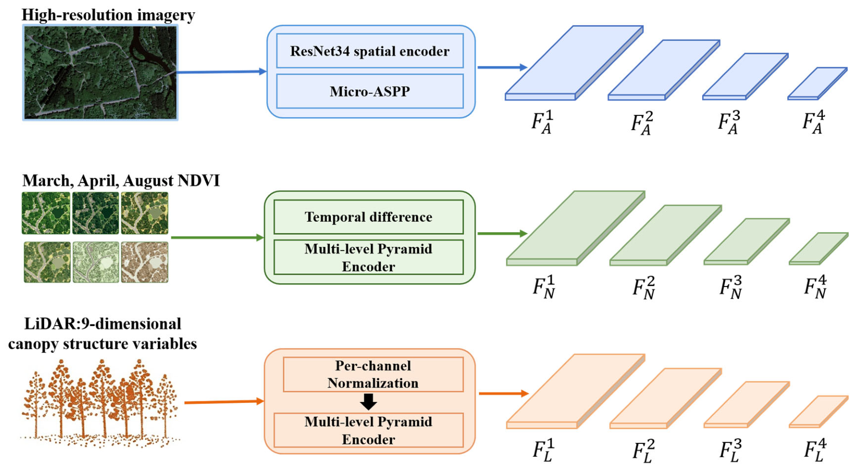
To extract discriminative information from each remote sensing modality, three parallel encoding branches are used for high-resolution imagery, NDVI phenological features, and LiDAR structural features before fusion (Figure 4). Let the August high-resolution image, multi-temporal NDVI features, and LiDAR structural features be denoted by $X_A$, $X_N$, and $X_L$, respectively, with corresponding encoders $E_A$, $E_N$, and $E_L$. Independent encoding produces feature maps at four scales for each modality:

$$\begin{array}{c}\left\{F_m^1,F_m^2,F_m^3,F_m^4\right\}=E_{m\left(X_m\right)},m\in \left\{A,N,L\right\}\end{array}$$

(1)

where $F_m^s$ denotes the representation of modality m at scale s. Compared with direct input-level concatenation, branch-specific encoding preserves the physical meaning of each modality before fusion: the high-resolution image represents crown texture and boundaries, NDVI captures phenological variation, and LiDAR characterizes three-dimensional canopy structure.

The high-resolution image branch uses a modified ResNet34 as the spatial feature-extraction backbone [45]. The first ResNet34 convolution is adapted to the multiband remote sensing input so that the August high-resolution image can be processed directly. The backbone progressively extracts shallow edge and texture features, intermediate local structures, and deep semantic information, yielding multiscale spatial features $\left\{F_A^1,F_A^2,F_A^3,F_A^4\right\}$. A lightweight Micro-ASPP module is appended to the highest-level feature to improve contextual representation of crown patches at different scales [46]. It aggregates multiscale context through a 1 × 1 convolution, 3 × 3 dilated convolutions with different dilation rates, and a global pooling branch, thereby enlarging the effective receptive field and strengthening deep semantic representations.

The NDVI phenology branch uses NDVI from March, April, and August and their temporal differences to describe changes in vegetation vigor from early-spring green-up to the stable growing season. A lightweight pyramid encoder first performs preliminary feature mapping and spatial downsampling in a stem module and then uses successive downsampling convolutions to derive multiscale phenological features $\left\{F_N^1,F_N^2,F_N^3,F_N^4\right\}$. The stem contains a 3 × 3 convolution–normalization–activation layer with stride 2 and a residual convolutional block. The former maps the input to 32 channels and performs initial spatial downsampling; the latter uses two 3 × 3 convolutions and a residual connection to enhance local phenological-change representations. This branch is more compact than the high-resolution image branch and focuses on temporal change patterns, helping distinguish species with similar crown appearance but different phenological rhythms.

The LiDAR structure branch takes nine canopy structural variables as input: maximum height, 95th-percentile height, mean height, height standard deviation, coefficient of variation in height, canopy relief ratio, canopy closure, gap fraction, and leaf area index. Each variable is normalized channel-wise before entering the model to reduce the effect of scale differences on network training. The LiDAR branch uses the same lightweight pyramid encoder as the NDVI branch and outputs multiscale structural features $\left\{F_L^1,F_L^2,F_L^3,F_L^4\right\}$. These three branches provide complementary spatial–textural, phenological, and canopy structural features before fusion, forming the basis for subsequent dynamic gated fusion.

3.2.2. Dynamic Gated Fusion of Spatial, Phenological, and Structural Features

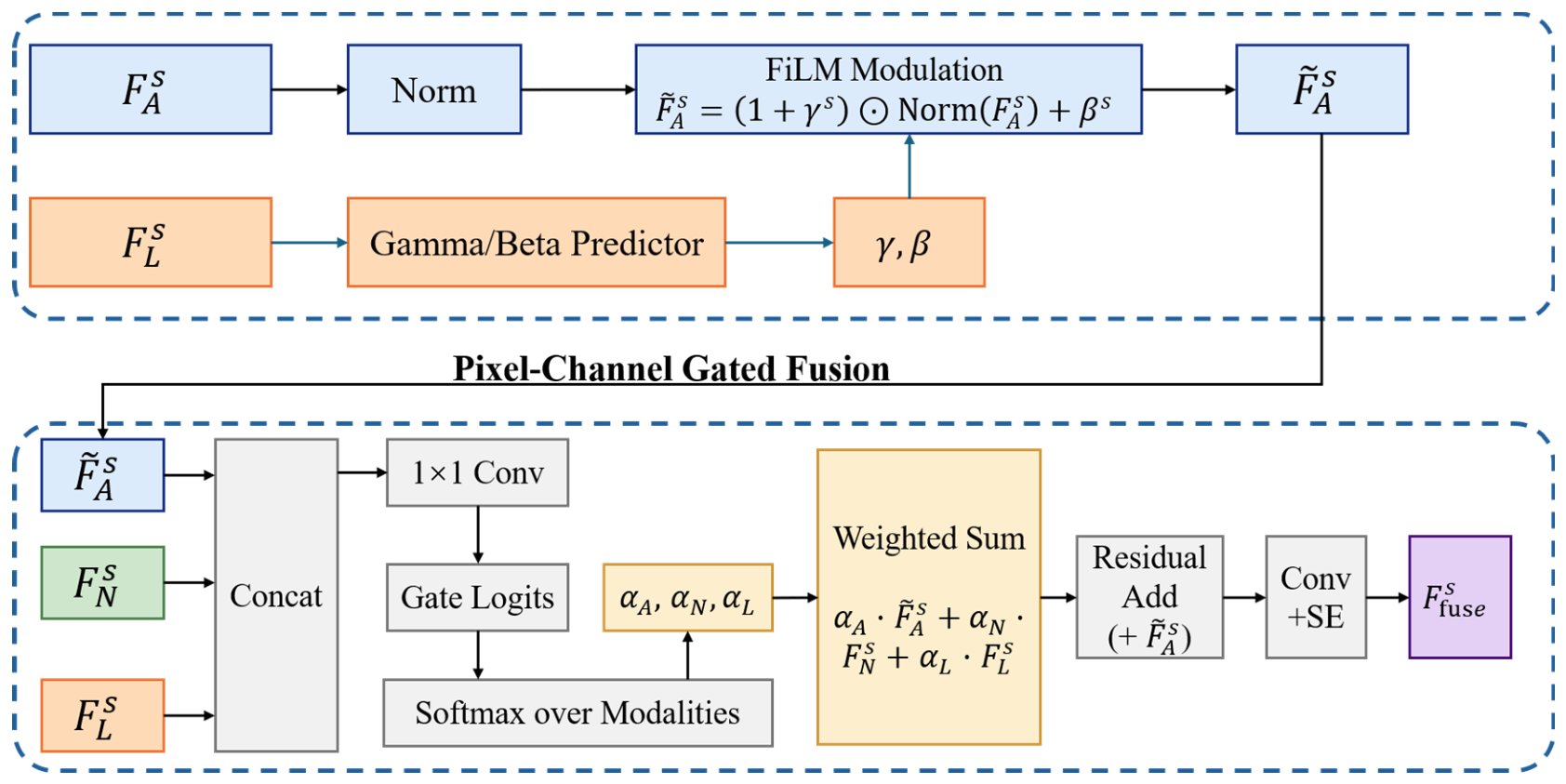
High-resolution image features, NDVI phenological features, and LiDAR structural features must be fused across multiple scales. Crown overlap, forest-edge shadows, mixed patches, and canopy structural variation are common in urban forests, the discriminative contribution of each modality varies spatially. We designed a dynamic gated fusion module that adaptively regulates modal contributions at each feature scale (Figure 5).

At scale s, let the high-resolution image feature, NDVI phenological feature, and LiDAR structural feature be $F_A^s$, $F_N^s$, and $F_L^s$, respectively, where $s\in \{1,2,3,4\}$. Before fusion, the three features are aligned to the same spatial dimensions so that modalities interact at corresponding pixel locations. Because LiDAR features are closely related to tree height, crown form, and spatial structure, we use a spatial FiLM modulation strategy [47]. LiDAR features at the same scale predict the scaling parameter ${\gamma }^s$ and offset parameter ${\beta }^s$, which are used to affinely transform the normalized high-resolution image feature:

$$\begin{array}{c}{\tilde{F}}_A^s=\left(1+{\gamma }^s\right)\odot Norm\left(F_A^s\right)+{\beta }^s\end{array}$$

(2)

where $\odot$ denotes element-wise multiplication and $\mathrm{N}\mathrm{o}\mathrm{r}\mathrm{m}\left(\cdot \right)$ denotes normalization. This operation allows LiDAR structural information to directly modulate the high-resolution image feature, imposing canopy structural constraints on crown texture and boundary representations. The module computes multi-modal fusion weights through joint pixel-channel gating. The three feature types are concatenated along the channel dimension, passed through a 1 × 1 convolution to generate gating responses, and normalized with Softmax over the modality dimension to obtain dynamic modal weights ${\alpha }_m^s$. The fused feature is expressed as:

$$\begin{array}{c}{F}_{fuse}^s\left(c,h,w\right)=\sum _{m\in \left\{A,N,L\right\}}{\alpha }_m^s\left(c,h,w\right)G_m^s\left(c,h,w\right)\end{array}$$

(3)

where ${\alpha }_m^s\left(c,h,w\right)$ is the weight of modality m at scale s, channel c, and spatial location (h, w). Joint spatial and channel constraints allow the model to adaptively select effective information sources according to local characteristics within crowns, at boundaries, in shadows, and in structurally distinct regions. To maintain the dominant role of high-resolution imagery in representing spatial detail, the gated fusion result is connected residually to the structure-modulated high-resolution image feature. Convolution and squeeze-and-excitation (SE) channel recalibration then produce the final fused feature:

$${\widehat{F}}^s=SE\left(Conv\left(F_{fuse}^s+{\tilde{F}}_A^s\right)\right)$$

(4)

The residual connection reduces training fluctuations caused by multi-modal fusion and prevents changes in auxiliary modality quality from excessively perturbing the backbone spatial feature. The SE module reallocates channel responses according to global context [48], enabling the fused feature to retain spatial texture, phenological differences, and structural constraints. During training, modality dropout randomly deactivates the NDVI or LiDAR auxiliary branch to reduce dependence on a single auxiliary modality and improve fusion robustness.

3.2.3. Reliability-Aware Hyperspectral–Semantic Prior Fusion

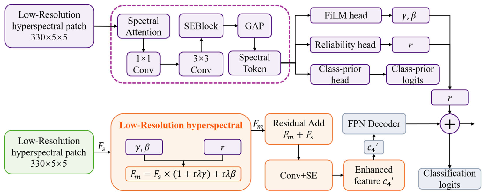
Hyperspectral imagery inherently possesses a lower spatial resolution than high-resolution imagery. Directly upsampling and concatenating it with high-resolution images, NDVI, and LiDAR features at shallow layers can introduce spatial ambiguity along canopy boundaries. To alleviate this scale discrepancy, we model the hyperspectral information as a spectral–semantic prior. Instead of fusing it with shallow boundary and textural features, we employ this prior for class-aware modulation within deep semantic features (Figure 6).

Let the hyperspectral input feature be $X_H$. Spatial global average pooling is first applied to $X_H$ to obtain a band descriptor representing the overall spectral response of the sample. A one-dimensional convolution and a multilayer perceptron then independently map this descriptor. The one-dimensional convolution captures local continuity between adjacent bands, whereas the multilayer perceptron learns discriminative global band combinations. Their responses are summed and passed through a Sigmoid function to generate band-attention weights, which are applied to the original hyperspectral feature:

$$X_H^{\prime }=X_H\odot \sigma \left(f_{1D}\left(GAP\left(X_H\right)\right)+f_{MLP}\left(GAP\left(X_H\right)\right)\right)$$

(5)

where $\odot$ denotes element-wise multiplication, $\sigma \left(\cdot \right)$ denotes the Sigmoid function, and $f_{1D}\left(\cdot \right)$ and $f_{MLP}\left(\cdot \right)$ denote one-dimensional convolutional and multilayer perceptron mappings, respectively. The weighted hyperspectral feature is processed by a lightweight encoder, global pooling, and an MLP to generate a spectral prior token ($t_H$) representing the overall spectral–semantic tendency of the current sample.

The spectral prior vector $t_H$ is further used to predict the FiLM modulation parameters: scaling parameter $\gamma$, offset parameter $\beta$, and reliability weight r. Let $F_H^4$ denote the highest-level semantic feature from multi-modal fusion on the high-resolution side. Reliability-aware modulation by the hyperspectral prior is then expressed as:

$${\widehat{F}}_H^4=F_H^4\odot \left(1+r\lambda \gamma \right)+r\lambda \beta$$

(6)

where $\lambda$ is a learnable modulation scale that controls the magnitude of the hyperspectral prior’s influence on deep features. The weight r represents the reliability of the hyperspectral prior for the current sample. When the HSI prior provides semantic information that is compatible with the high-resolution-side representation, a larger r permits stronger modulation. Conversely, when the HSI information is unstable or has insufficient spatial specificity, a smaller r reduces its influence, thereby limiting interference from the coarse-resolution prior in pixel-level boundary discrimination. r provides an implicit assessment of cross-modal compatibility while preserving the high-resolution features as the primary source of spatial and boundary information. The hyperspectral prior acts primarily on the highest-level semantic feature to enhance spectral discrimination at the class level. In addition to FiLM modulation, the hyperspectral branch produces class prior logits that enter the final prediction as a class-level bias. Modality dropout is also applied to the hyperspectral prior branch during training to reduce dependence on a single low-resolution spectral source and improve the stability of multi-source fusion.

3.2.4. Multiscale Decoder and Loss Functions

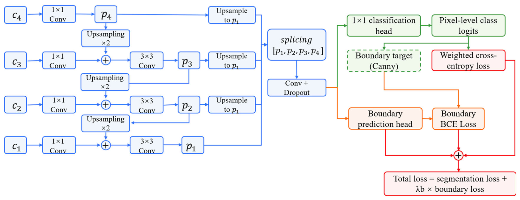
HybridFusion uses an FPN decoder to produce pixel-level tree species predictions [49], as shown in Figure 7. Let the four scale-specific outputs of the fusion module be $c_1$, $c_2$, $c_3$, and $c_4$. The decoder first uses 1 × 1 convolutions to standardize their channel dimensions. A top-down pathway then progressively upsamples high-level semantic features and laterally fuses them with lower-level spatial features to form multiscale decoded features:

$$p_s=Conv\left(c_s+Up\left(p_{s+1}\right)\right),s=1,2,3$$

(7)

where $p_s$ denotes the decoded feature at scale s, $\mathrm{U}\mathrm{p}\left(\cdot \right)$ is the upsampling operation, and $\mathrm{C}\mathrm{o}\mathrm{n}\mathrm{v}\left(\cdot \right)$ is convolutional smoothing. Subsequently, $p_2$, $p_3$, and $p_4$ are upsampled to the spatial dimensions of $p_1$ and concatenated with $p_1$ along the channel dimension. After convolution, Dropout, and the classification head, the final class logits are obtained:

$$\begin{array}{c}P={Conv}_{1\times 1}\left(\Phi \left(\left[p_1,Up\left(p_2\right),Up\left(p_3\right),Up\left(p_4\right)\right]\right)\right)\end{array}$$

(8)

where $\Phi \left(\cdot \right)$ denotes the convolutional fusion module. Model training jointly optimizes the primary classification loss and an auxiliary boundary loss. The primary loss is a class-weighted cross-entropy loss:

$$\begin{array}{c}{\mathcal{L}}_{seg}=CE\left(P,Y;w\right)\end{array}$$

(9)

where P denotes the predicted class logits, Y is the reference label, and w is the class weight used to mitigate sample imbalance between the Non-tree background and individual tree species. Invalid pixels and ignored regions are masked during loss computation so that low-confidence labels do not influence model optimization. An auxiliary boundary branch is attached to the decoder to improve discrimination along crown outlines and adjacent class boundaries [50]. It takes the final decoded feature as input and produces a single-channel boundary prediction. Reference boundaries are automatically generated from the label map by identifying class changes between neighboring pixels within the valid region and moderately dilating the resulting boundary. The branch is supervised with a positive-class-weighted binary cross-entropy loss to reduce training bias caused by the small number of boundary pixels. The final training objective is:

$$\mathcal{L}={\mathcal{L}}_{seg}+{\lambda }_b{\mathcal{L}}_{boundary}$$

(10)

where ${\mathcal{L}}_{boundary}$ is the auxiliary boundary loss and ${\lambda }_b$ is its weight, set to 0.2 in this study [51]. The joint loss retains tree species pixel classification as the primary objective while constraining feature learning at crown interfaces through boundary supervision, thereby reducing local misclassification and boundary confusion.

4. Experimental Design and Results

4.1. Experimental Setup and Ablation Design

The model and all additional baseline models were implemented in PyTorch version 2.2.1 and trained on the same NVIDIA RTX 4070 GPU using 20 × 20 pixel label patches. The AdamW optimizer was employed with an initial learning rate of 0.001 and a weight decay of 0.0001. The learning rate was adjusted using cosine annealing over 100 epochs, with a batch size of 128 [52]. The total loss combined class-weighted cross-entropy and an auxiliary boundary loss, for which the loss weight and dilation radius were set to 0.2 and 1, respectively. Overall accuracy (OA), tree species OA (Tree OA), the Kappa coefficient, mean Intersection over Union (mIoU), and Macro-F1 were used as evaluation metrics, and the checkpoint with the highest validation Tree OA was selected. As summarized in

Table 3. Experimental design for assessing data source contributions.

Exp.	Input Data	Description
Exp. 1	August high-resolution imagery	Spatial texture baseline for assessing the tree species classification capability of high-resolution imagery
Exp. 2	High-resolution imagery and March/April/August NDVI	Assess the contribution of multi-temporal phenological information
Exp. 3	High-resolution imagery and LiDAR structural features	Assess the contribution of three-dimensional LiDAR structural information
Exp. 4	High-resolution imagery, NDVI, and LiDAR	Assess joint modeling of phenological and canopy structural features
Exp. 5	High-resolution imagery and HSI semantic prior	Assess the independent contribution of the low-spatial-resolution hyperspectral prior
Exp. 6	High-resolution imagery, NDVI, LiDAR, and HSI	HybridFusion model for assessing integrated multi-source fusion

,

Table 4. Experimental design for comparing high-resolution-side fusion strategies.

Exp.	High-Resolution-Side Fusion Strategy	Description
Exp. 7	Input-level stacking	Directly concatenate high-resolution imagery, NDVI, and LiDAR along the channel dimension before input to the spatial encoder
Exp. 8	Feature-level concatenation	Encode the three feature types separately, then concatenate and reduce their dimensions for fusion
Exp. 4	Dynamic gated fusion	Adaptively fuse multi-source high-resolution-side features using LiDAR spatial FiLM modulation and joint pixel-channel gating

and

Table 5. Experimental design for comparing hyperspectral–semantic prior fusion strategies.

Exp.	HSI Fusion Strategy	Description
Exp. 4	No HSI prior	Use only high-resolution imagery, NDVI, and LiDAR as the baseline for HSI fusion experiments
Exp. 9	Spatial bias prior	Add the HSI encoding as a coarse-scale spatial bias to deep semantic features
Exp. 10	FiLM modulation prior	Use the HSI branch to generate channel-modulation parameters and apply FiLM to deep fused features
Exp. 11	Class prior	Add only the class prior logits from the HSI branch to the final classification output
Exp. 12	No reliability gating	Retain the HSI semantic prior but introduce hyperspectral information with a fixed weight
Exp. 6	Reliability-aware semantic prior	Fuse the HSI prior using spectral attention, HSI-based FiLM modulation, a class prior, and reliability gating

, three groups of experiments were designed to systematically evaluate data source contributions and fusion strategies:

(1) Data source contributions (Exps. 1–6): Evaluated single-source versus multi-source classification. Exp. 1 served as the baseline (August high-resolution image only). Exps. 2–5 progressively introduced NDVI, LiDAR, and HSI priors to assess their independent and joint contributions, culminating in Exp. 6, which represented the complete HybridFusion model with all modalities.

(2) High-resolution fusion strategies (Exps. 7, 8, and 4): Compared input-level stacking, feature-level fusion, and dynamic gated fusion (the no-HSI baseline), respectively, to determine the optimal joint representation mechanism for spatial, phenological, and structural features.

(3) Hyperspectral prior ablations (Exps. 4, 9–12, and 6): Using Exp. 4 as a baseline, these experiments compared spatial bias, FiLM channel-modulation, class prior, ungated-reliability, and reliability-aware configurations to validate the effectiveness of hyperspectral–semantic guidance and reliability control.

To provide an architecture-level comparison under identical information availability, four external baselines were additionally implemented: FullModal-U-Net, FullModal-DeepLabV3+, FullModal-FPN, and MultiModal-Concat. Each model received four-channel high-resolution imagery, two-channel multi-temporal NDVI, nine-channel LiDAR structural features, and a 330-band HSI patch. For FullModal-U-Net, FullModal-DeepLabV3+, and FullModal-FPN, an identical lightweight HSI adapter projected the hyperspectral input from 330 to 32 and subsequently to 8 channels using two 1 × 1 convolutional layers. The resulting features were bilinearly upsampled and concatenated with the high-resolution imagery, NDVI, and LiDAR features before being processed by the corresponding segmentation backbone. MultiModal-Concat independently encoded the four modalities and concatenated their features at a common spatial resolution before classification. Except for architecture-specific fusion and regularization components, all models used the same data partition, preprocessing procedure, optimizer, learning-rate schedule, number of epochs, batch size, loss functions, checkpoint-selection criterion, and evaluation metrics.

4.2. Results

4.2.1. Separability of Multi-Source Remote Sensing Features

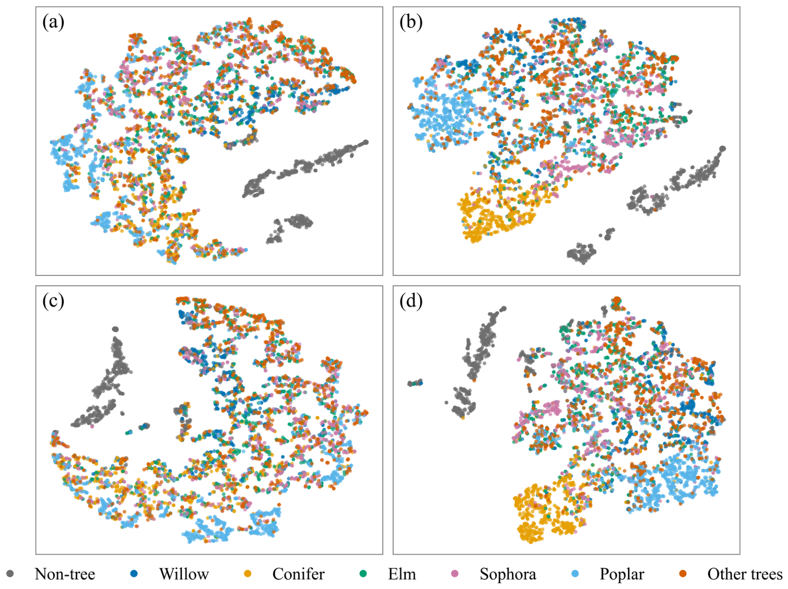
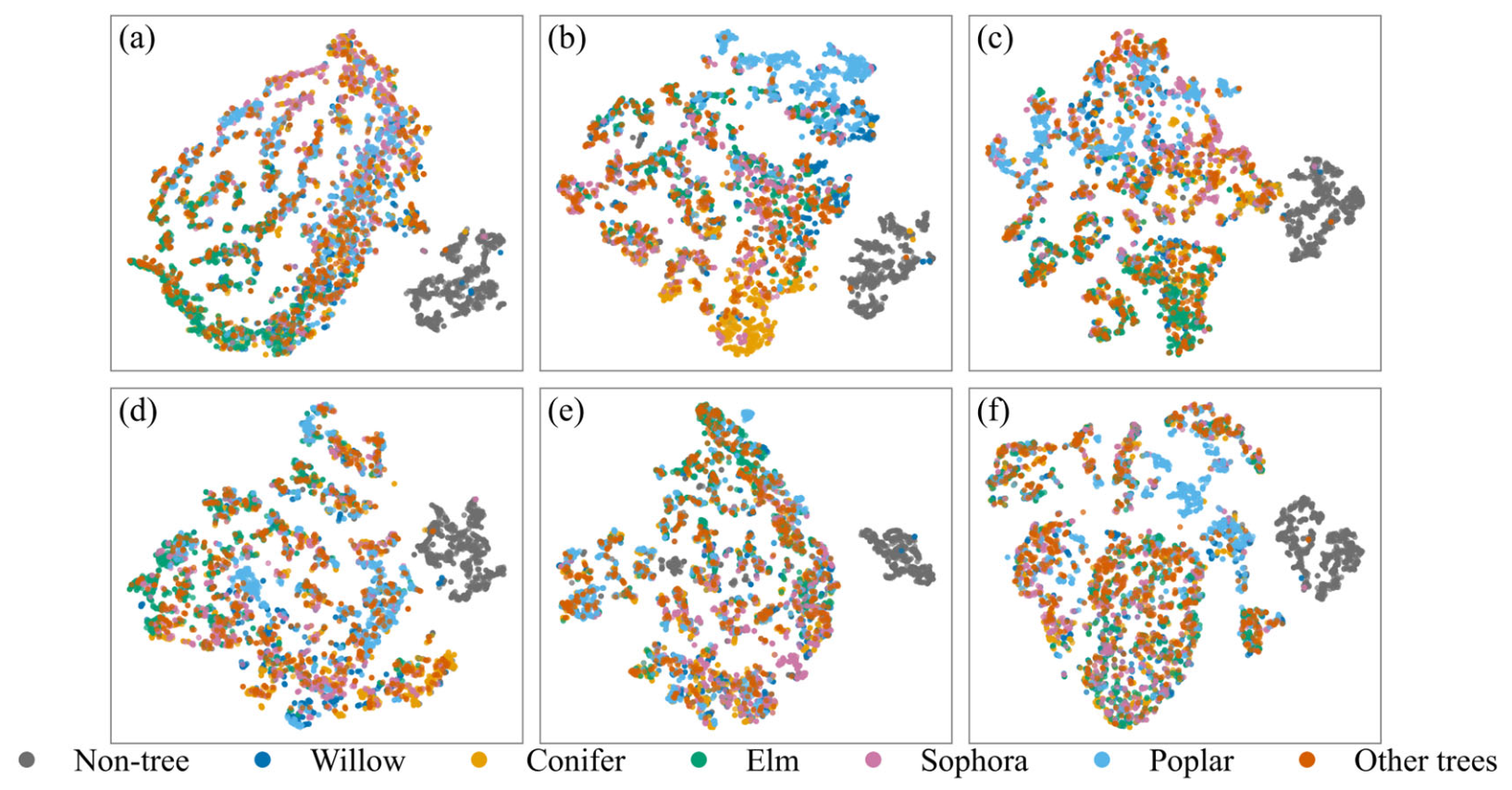
To examine how multi-source remote sensing information affects tree species discrimination, we evaluated feature separability at two levels: original input features and deep fused features learned by the model. Using valid pixels from the training and validation sets, four original feature combinations were constructed: high-resolution imagery alone, high-resolution imagery + NDVI, high-resolution imagery + LiDAR, and high-resolution imagery + NDVI + LiDAR. After standardization and preliminary dimensionality reduction with PCA, each feature set was mapped to two-dimensional space using t-SNE to represent class clustering and overlap. The silhouette coefficient, Davies–Bouldin (DB) index, and Calinski–Harabasz (CH) index were also used for quantitative evaluation. Higher silhouette and CH values and a lower DB value generally indicate stronger class separability. The t-SNE visualizations of the original feature space are shown in Figure 8, and the quantitative results are listed in

Table 6. Evaluation of original feature separability.

Feature Combination	Sample Count	Silhouette Coefficient	DB Index	CH Index
Original high-resolution imagery	3011	−0.1260	5.4952	186.96
High-resolution imagery + NDVI	3011	−0.0492	3.2514	248.30
High-resolution imagery + LiDAR	2915	−0.1139	5.5924	65.05
High-resolution imagery + NDVI + LiDAR	2915	−0.0464	3.2847	101.36

.

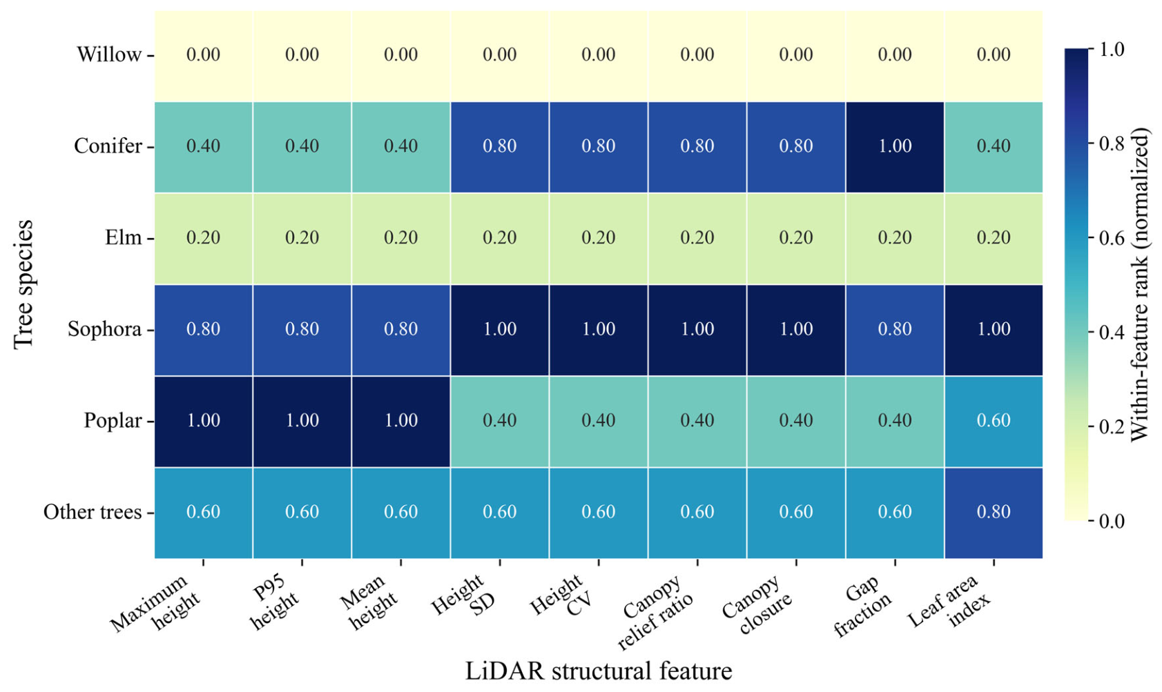
Figure 8 and Table 6 show that the use of high-resolution imagery alone leads to substantial overlap among tree species in feature space. The boundaries of broadleaf classes, including Willow, Elm, Sophora, and Other trees, are particularly indistinct. The silhouette coefficient is −0.1260 and the DB index is 5.4952, indicating that a single-date high-resolution image can represent crown texture and local spatial morphology but has limited ability to separate fine-grained tree species classes. After multi-temporal NDVI is introduced, the organization of the feature space improves markedly: the silhouette coefficient increases to −0.0492, the DB index decreases to 3.2514, and the CH index increases from 186.96 to 248.30. These changes indicate that phenological information enhances interspecies feature differences. LiDAR structural features complement optical imagery primarily through canopy height and vertical structure. Although the high-resolution imagery + LiDAR combination does not achieve the best global clustering indices in the original feature space, the class-mean heat map of LiDAR structural features (Figure 9) shows that Poplar differs substantially in maximum height, mean height, canopy closure, and leaf area index. Thus, structural information helps distinguish species with pronounced crown morphology. When NDVI and LiDAR are jointly introduced, the silhouette coefficient further increases to −0.0464, demonstrating complementarity between phenological and structural features in representing interspecies differences.

To further assess feature organization after model learning, we extracted deep encoding features from the best model of each experiment and visualized them using t-SNE (Figure 10 and

Table 7. Separability evaluation of representative deep features.

Exp.	Silhouette Coefficient	DB Index	CH Index
Exp. 1: high-resolution imagery only	−0.1348	6.1039	49.82
Exp. 2: high-resolution imagery + NDVI	−0.0877	5.0273	79.97
Exp. 3: high-resolution imagery + LiDAR	−0.0704	6.1390	77.44
Exp. 4: high-resolution imagery + NDVI + LiDAR	−0.0910	4.5230	51.68
Exp. 6: full-modality reliability-aware HSI semantic prior	−0.0836	6.4126	45.19

). Compared with the original features, deep features learned under supervision are more closely aligned with the classification objective and no longer depend on a single spectral, phenological, or structural difference. Adding NDVI clarifies the class distribution relative to the baseline. Feature-level fusion and dynamic fusion can adjust interclass distances to some extent. After the hyperspectral prior is introduced, the global clustering indices do not improve monotonically, indicating that its principal role is semantic correction for complex samples and locally confused regions. Overall, multi-source remote sensing features enhance tree species representation through phenological variation, canopy structure, and spectral semantics, establishing a feature basis for improved classification accuracy.

4.2.2. Accuracy of the Full-Modality Model

To further evaluate class-level performance of the full-modality HybridFusion model, the best result from Experiment 6 is summarized in

Table 8. Class-level evaluation results for the best experiment.

Class	IoU/%	F1/%	UA/%	PA/%	Validation Pixel Count
Non-tree	97.21	98.58	100.00	97.21	2113
Willow	75.86	86.27	92.34	80.96	625
Conifer	73.76	84.90	84.66	85.14	175
Elm	64.72	78.58	73.89	83.91	435
Sophora	68.14	81.05	86.80	76.02	467
Poplar	91.04	95.31	93.13	97.60	125
Other trees	74.44	85.35	79.65	91.93	830

. Overall, the full-modality model achieved stable classification performance for the Non-tree class and the major tree species. The Non-tree class achieved an F1 score of 98.58% and an IoU of 97.21%, indicating effective separation of crown areas from roads, water bodies, grassland, and buildings. Among tree species, Poplar achieved the best result, with an F1 score of 95.31% and PA of 97.60%. Its pronounced canopy structure and spatial morphology provide high separability after multi-source fusion. F1 scores for Willow, Conifer, and Other trees were 86.27%, 84.90%, and 85.35%, respectively, indicating that phenological, structural, and spectral–semantic information effectively supports recognition of the principal tree species.

Differences in UA and PA across species reveal distinct error patterns. Willow attained a UA of 92.34%, exceeding its PA of 80.96%, indicating high reliability of Willow predictions but some omission errors. Conifer achieved balanced performance, with UA and PA of 84.66% and 85.14%, respectively. Elm had the lowest F1 score among tree species (78.58%) and a UA of only 73.89%, indicating residual confusion with other broadleaf species in crown texture and phenological response. Sophora achieved an F1 score of 81.05% and a PA of 76.02%, suggesting some omission errors that may be related to crown interlacing in mixed stands and within-class sample variation. Other trees achieved a PA of 91.93% but a UA of 79.65%. This class combines multiple species with small sample sizes and scattered distributions, resulting in strong within-class heterogeneity and a tendency to absorb predictions from similar broadleaf species. Overall, HybridFusion performs well for major tree species, but Elm, Sophora, and Other trees remain priority classes for further improvement in fine-grained classification.

4.2.3. Comparison with Representative Full-Modality Baselines

Under the unified full-modality setting, FullModal-FPN was the strongest of the three conventional semantic segmentation backbones, achieving an OA of 89.64%, a Tree OA of 82.35%, a Kappa coefficient of 0.8593, an mIoU of 74.19%, and a Macro-F1 of 84.73%. Compared with FullModal-U-Net, FullModal-FPN improved Tree OA, mIoU, and Macro-F1 by 4.10, 4.44, and 3.54 percentage points, respectively (

Table 9. Accuracy comparison under the unified full-modality setting.

Model	OA (%)	Tree OA (%)	Kappa	mIoU (%)	Macro-F1 (%)
FullModal-U-Net	87.30	78.25	0.8274	69.75	81.19
FullModal-DeepLabV3+	86.50	76.59	0.8166	68.87	80.40
FullModal-FPN	89.64	82.35	0.8593	74.19	84.73
MultiModal-Concat	88.78	80.39	0.8476	72.05	83.11
HybridFusion	90.44	85.06	0.8707	77.88	87.15

). Compared with FullModal-DeepLabV3+, the corresponding improvements were 5.76, 5.32, and 4.33 percentage points. MultiModal-Concat achieved a Tree OA of 80.39%, indicating that direct feature concatenation can exploit complete multi-modal inputs but provides limited adaptive intermodal interaction.

HybridFusion achieved the highest values for all evaluation metrics, with an OA of 90.44%, a Tree OA of 85.06%, a Kappa coefficient of 0.8707, an mIoU of 77.88%, and a Macro-F1 of 87.15%. Relative to FullModal-FPN, HybridFusion improved Tree OA, mIoU, and Macro-F1 by 2.71, 3.69, and 2.42 percentage points, respectively. Because all models received the complete set of remote sensing sources, these results indicate that the improvement of HybridFusion is not attributable solely to the inclusion of HSI data. Instead, the results support the effectiveness of dynamic multi-modal fusion and reliability-aware hyperspectral–semantic prior modeling.

4.2.4. Computational Complexity and Inference Efficiency

The computational complexity and inference efficiency of the five full-modality models were further evaluated. Parameter count and FLOPs were calculated for the complete inference graph, including the HSI-processing components. All inference measurements were performed on the same NVIDIA RTX 4070 GPU using FP32 inference, a batch size of 1, five warm-up iterations, and 30 timed iterations.

MultiModal-Concat had the smallest parameter count and lowest latency, with 0.507 M parameters and a mean latency of 1.349 ms (

Table 10. Computational complexity and inference efficiency.

Model	Parameters (M)	GFLOPs	FP32 Size (MB)	Latency (ms)	Throughput (Patch/s)	Peak GPU Memory (MB)
FullModal-U-Net	1.965	2.153	7.50	1.752	570.71	162.57
FullModal-DeepLabV3+	1.633	0.854	6.23	1.566	638.61	31.17
FullModal-FPN	1.258	1.262	4.80	1.468	681.23	151.28
MultiModal-Concat	0.507	2.515	1.93	1.349	741.55	29.11
HybridFusion	40.061	3.915	152.82	14.800	67.57	294.14

). FullModal-DeepLabV3+ had the lowest theoretical computational cost among the three conventional segmentation backbones, requiring 0.854 GFLOPs. FullModal-FPN provided the most favorable accuracy–efficiency balance, requiring 1.258 M parameters and 1.262 GFLOPs while achieving a mean latency of 1.468 ms and a throughput of 681.23 patches/s. HybridFusion required 40.061 M parameters and 3.915 GFLOPs, with a mean latency of 14.800 ms. Compared with FullModal-FPN, HybridFusion used approximately 31.8 times as many parameters, 3.1 times the FLOPs, and 10.1 times the measured latency while improving Tree OA by 2.71 percentage points and mIoU by 3.69 percentage points. HybridFusion therefore trades greater computational cost for improved fine-grained classification accuracy.

4.3. Spatial Distribution Patterns of Tree Species

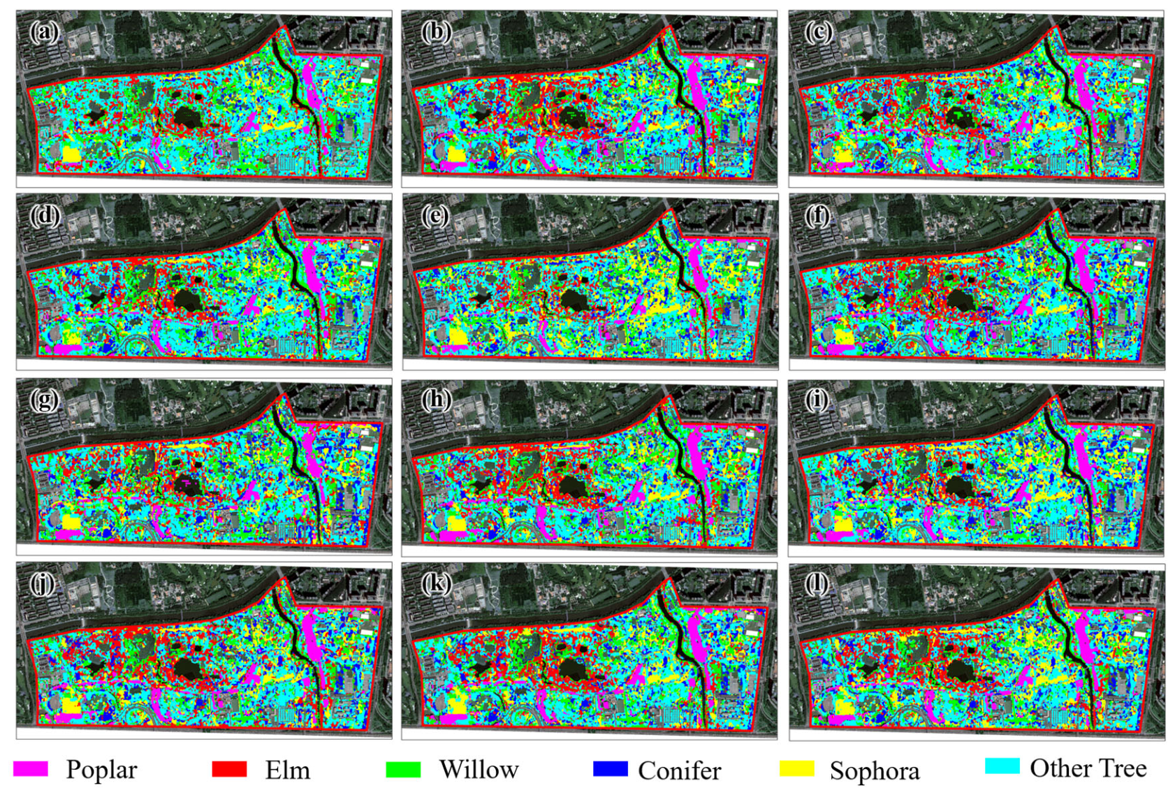
To transfer the tree species classification model trained at the sample scale to the full study area, we performed study area-wide mapping using overlapping sliding-window inference. High-resolution imagery served as the common spatial reference, and the corresponding high-resolution imagery, multi-temporal NDVI, LiDAR structural features, and HSI semantic priors were read for each window. Each experiment activated or masked input branches according to its modality configuration, ensuring consistency in spatial extent, class scheme, and inference workflow across the 12 classification results. The final outputs comprised seven classes: Non-tree, Willow, Conifer, Elm, Sophora, Poplar, and Other trees. To reduce the effect of unstable predictions near sliding-window edges on the full-image classification result, Gaussian-weighted fusion was applied across overlapping windows. Let the output-window side length be L, the relative pixel coordinate within a window be (i, j), and the window-center coordinate be $c=(L-1)/2$. The two-dimensional Gaussian weight is defined as:

$$G\left(i,j\right)=\mathit{exp}\left\{-{\displaystyle \frac{\left[{\left(i-c\right)}^2+{\left(j-c\right)}^2\right]}{2{\sigma }^2}}\right\},\sigma ={\displaystyle \frac{L}{6}}$$

(11)

To combine predictions from different windows, the Gaussian weights are normalized as:

$$\tilde{G}\left(i,j\right)={\displaystyle \frac{G\left(i,j\right)}{max\left(G\right)}}$$

(12)

For any pixel x in the full image that is covered by multiple sliding windows, let K(x) be the set of windows covering x and let p_k,_m(x) be the probability for class m predicted by the kth window. The fused class probability at that pixel is then:

$${\overline{p}}_m\left(x\right)={\displaystyle \frac{\sum _{k\in K\left(x\right)}{\tilde{G}}_k\left(x\right)p_{k,m}\left(x\right)}{\sum _{k\in K\left(x\right)}{\tilde{G}}_k\left(x\right)}}$$

(13)

The final class is determined by the maximum fused probability:

$$\hat{\mathrm{y}}\left(x\right)=argma{x}_{\mathrm{m}}{\overline{p}}_{\mathrm{m}}\left(x\right)$$

(14)

This strategy improves prediction continuity in overlapping regions, yielding more stable spatial representation at stand boundaries and within patches in the study area-wide classification map (Figure 11).

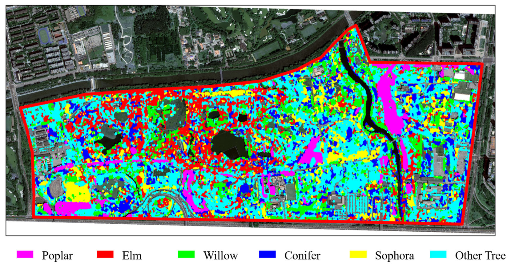
Using the best-performing HybridFusion model in the integrated evaluation, we further analyzed tree species spatial distribution in the northern section of Olympic Forest Park (Figure 12). Based on the 2 m classification grid, the effective study area is approximately 310.85 ha, including 175.12 ha of tree-covered area (56.34%) and 135.73 ha of Non-tree area (43.66%). The percentages of tree-covered and Non-tree areas were calculated relative to the total effective study area, whereas the species-level percentages were calculated relative to the total tree-covered area. Other trees occupy the largest tree-covered area, covering 67.69 ha or 38.65% of the total tree-covered area. Elm, Willow, and Conifer cover 27.77, 25.81, and 23.56 ha, accounting for 15.86%, 14.74%, and 13.45%, respectively. Sophora and Poplar cover 17.74 and 12.55 ha, accounting for 10.13% and 7.17%, respectively.

Spatially, the tree species distribution reflects characteristic patterns of urban mixed forests and landscape planting. The “Other trees” class dominates the areal coverage, highlighting the prevalence of diverse ornamental species and complex mixed patches beyond the primary targets. This inherent compositional complexity makes it a highly heterogeneous target for remote sensing classification. Willows predominantly form belts along water bodies, aligning with typical riparian planting strategies. Conifers cluster to form localized, contiguous evergreen stands. In contrast, poplars cover a minor area and are largely confined to distinct linear patterns along roadsides and forest edges. Elms and Sophoras are spatially dispersed, frequently occurring within mixed interior stands or roadside greenspaces, thereby epitomizing the highly intermixed broadleaf structures typical of urban forests.

4.4. Comparison of Classification Results in Representative Areas

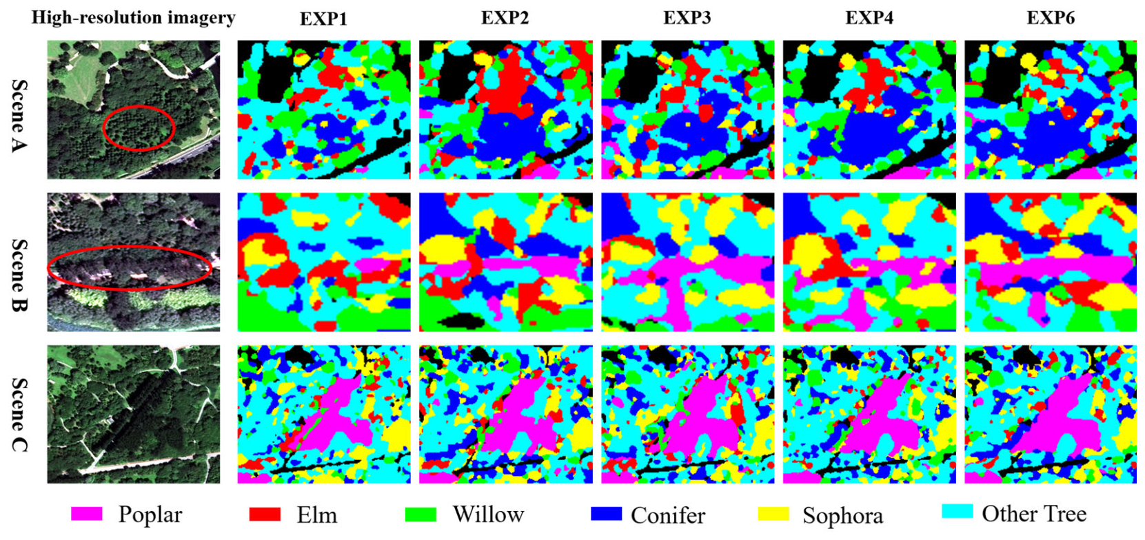
To visually evaluate the impact of multi-source data fusion on fine-scale classification, three representative local scenes were selected (Figure 13): a contiguous Conifer patch (Scene A), a linear roadside Poplar belt (Scene B), and a complex broadleaf mixed forest (Scene C).

Scene A is a Conifer forest patch. When only high-resolution imagery is used, Conifer predictions are fragmented and some locations are misclassified as Elm, Willow, or Other trees. This result indicates that a single-date high-resolution image can represent crown texture and color differences but cannot reliably separate the Conifer class from neighboring broadleaf species. After NDVI is introduced, predicted Conifer areas correspond more closely to Conifer canopy locations in the imagery; mixed predictions of broadleaf species within patches decrease, and both spatial continuity and class purity improve. After LiDAR structural features and the HSI semantic prior are incorporated, the main Conifer area remains spatially continuous, indicating that phenological, canopy structural, and spectral–semantic information jointly improves the reliability of evergreen forest patch recognition.

Scene B is a roadside Poplar stand and tall-tree belt, where crowns are distributed linearly along roads and forest edges. With high-resolution imagery alone or combined with NDVI, the target area still contains mixed predictions of Elm, Sophora, and Other trees, and the Poplar map lacks continuity. After LiDAR structural features are introduced, Poplar’s roadside linear distribution becomes clearer and more consistent with the actual location of the tall-tree belt. This finding indicates that structural information such as tree height, canopy relief, and canopy closure provides effective constraints for recognizing species with distinctive canopy structure. The full-modality HybridFusion model preserves the linear spatial pattern while reducing locally fragmented misclassification, producing a more complete classification of roadside tree belts.

Scene C is a complex broadleaf mixed forest containing Willow, Elm, Sophora, and Other trees. Crown overlap, forest-edge shadows, and mosaic species distributions are pronounced. With high-resolution imagery alone, predictions contain numerous scattered patches and some class boundaries correspond inconsistently to actual crown structure. Adding NDVI and LiDAR improves local spatial continuity, but confusion persists among Elm, Sophora, and Other trees. By jointly leveraging phenological variation, canopy structure, and hyperspectral–semantic information, the full-modality model improves class continuity and reduces local errors across spatial contexts; nevertheless, fine-grained discrimination within complex broadleaf mixed forests remains highly uncertain.

5. Discussion

5.1. Complementary Contributions of the Remote Sensing Sources

Twelve comparative experiments were conducted to evaluate the effects of multi-source remote sensing features and fusion strategies on urban forest tree species classification. The experiments cover three aspects: data source contributions, high-resolution-side fusion strategies, and hyperspectral–semantic prior fusion strategies. All experiments used the same data partition, training parameters, and evaluation protocol; integrated results are reported in

Table 11. Integrated evaluation results for the 12 experiments.

Exp.	Data and Fusion Strategy	OA/%	Tree OA/%	Kappa	mIoU/%	Macro-F1/%
Exp. 1	High-resolution imagery only	80.23	67.29	0.7315	58.58	71.35
Exp. 2	High-resolution imagery + NDVI	84.59	76.06	0.7924	69.38	80.45
Exp. 3	High-resolution imagery + LiDAR	86.46	76.63	0.8162	65.49	78.14
Exp. 4	High-resolution imagery + NDVI + LiDAR	89.25	81.90	0.8540	71.95	82.94
Exp. 5	High-resolution imagery + HSI semantic prior	81.13	68.65	0.7430	60.49	73.65
Exp. 6	Full-modality reliability-aware HSI semantic prior	90.44	85.06	0.8707	77.88	87.15
Exp. 7	High-resolution-side input-level stacking	84.11	72.53	0.7836	63.16	75.68
Exp. 8	High-resolution-side feature-level concatenation	88.32	80.50	0.8419	72.91	83.47
Exp. 9	HSI spatial bias prior	89.52	81.71	0.8573	75.88	85.51
Exp. 10	HSI channel-modulation prior	88.72	80.81	0.8470	71.61	82.74
Exp. 11	HSI class prior	89.20	83.21	0.8540	72.79	83.63
Exp. 12	Fixed-reliability HSI semantic prior	89.71	82.35	0.8601	73.95	84.55

. The full-modality HybridFusion model (Experiment 6) achieved the best performance, with OA, Tree OA, Kappa, mIoU, and Macro-F1 of 90.44%, 85.06%, 0.8707, 77.88%, and 87.15%, respectively. This result demonstrates that synergistic modeling of spatial texture, phenological variation, canopy structure, and spectral semantics improves fine-grained tree species classification in complex urban forests [26,27,33].

5.1.1. Individual and Combined Contributions of Multi-Source Remote Sensing Data

The gains from different remote sensing modalities vary substantially (

Table 12. Performance gains in the data source contribution experiments.

Comparison with Exp. 1	OA Gain/%	Tree OA Gain/%	mIoU Gain/%	Tree mIoU Gain/%
Exp. 2	4.36	8.77	10.80	12.75
Exp. 3	6.23	9.33	6.91	7.60
Exp. 4	9.01	14.60	13.37	15.19
Exp. 5	0.90	1.35	1.91	2.15
Exp. 6	10.21	17.76	19.30	22.30

). With high-resolution imagery alone, the model achieved a Tree OA of 67.29%. A single-date high-resolution image thus represents crown boundaries, canopy color, and texture but remains limited in separating species with similar crown form and spectral response in urban mixed forests. Adding NDVI increased Tree OA to 76.06%, an improvement of 8.77 percentage points over the baseline, demonstrating that multi-temporal phenological information enhances species discrimination, particularly between evergreen Conifer and deciduous broadleaf species [53]. Adding LiDAR yielded a Tree OA of 76.63%, indicating that canopy height, relief, closure, and related structural attributes complement vertical differences that cannot be represented adequately in two-dimensional optical imagery [20].

When NDVI and LiDAR were jointly used, Tree OA further increased to 81.90%, 14.60 percentage points above the high-resolution-only baseline, confirming complementarity between phenological variation and canopy structure. The independent gain from the HSI semantic prior was modest. In contrast, the full-modality HybridFusion model achieved a Tree OA of 85.06%, an improvement of 17.76 percentage points over the baseline. Hyperspectral semantics therefore function more effectively as a deep complement to spatial texture, phenology, and structure than as a substitute for high-resolution spatial information.

Table 13. Classification accuracy across data source combinations.

Accuracy Metric	Exp. 1	Exp. 2	Exp. 3	Exp. 4	Exp. 5	Exp. 6
Tree OA/%	67.29	76.06	76.63	81.90	68.65	85.06
Kappa × 100	73.15	79.24	81.62	85.40	74.30	87.07
Willow F1/%	81.38	84.33	79.85	89.79	78.13	86.27
Conifer F1/%	50.34	76.84	62.61	73.98	65.00	84.90
Elm F1/%	52.67	59.79	70.15	75.08	54.33	78.58
Sophora F1/%	60.29	70.02	72.71	72.00	64.05	81.05
Poplar F1/%	91.77	98.79	81.20	86.69	88.99	95.31
Other trees F1/%	65.07	75.99	81.10	83.90	66.89	85.35

further shows changes in species-specific F1 scores across data source combinations. NDVI produced pronounced gains for Conifer and Poplar: Conifer F1 increased from 50.34% to 76.84%, and Poplar F1 reached 98.79%. LiDAR provided useful complementary information for Elm, Sophora, and Other trees. Full-modality fusion attained the highest or near-highest F1 scores for Conifer, Elm, Sophora, and Other trees, at 84.90%, 78.58%, 81.05%, and 85.35%, respectively. These results indicate that synergistic use of phenological, structural, and spectral–semantic information mitigates fine-grained species confusion in urban mixed forests.

5.1.2. Integration Strategies for High-Resolution, Phenological, and LiDAR Information

To assess the dynamic gated fusion module on the high-resolution side, input-level stacking and feature-level concatenation were used as comparators, and the dynamic gated model without the HSI prior (Experiment 4) represented the proposed high-resolution-side fusion strategy.

Table 14. Comparison of high-resolution-side fusion strategies.

Fusion Strategy	Corresponding Exp.	OA/%	Tree OA/%	mIoU/%	Macro-F1/%
Input-level stacking	Exp. 7	84.11	72.53	63.16	75.68
Feature-level concatenation	Exp. 8	88.32	80.50	72.91	83.47
Dynamic gated fusion	Exp. 4	89.25	81.90	71.95	82.94

shows that input-level stacking achieved a Tree OA of 72.53%, lower than both feature-level concatenation and dynamic gated fusion. Directly concatenating high-resolution imagery, NDVI, and LiDAR at the input layer is therefore susceptible to differences in modal scale and noise distribution and cannot fully exploit source complementarity. By encoding the three sources in separate branches before fusion, feature-level concatenation increased Tree OA to 80.50%, indicating that feature-level fusion reduces the redundancy associated with direct stacking [54,55].

Dynamic gated fusion achieved the highest OA and Tree OA, at 89.25% and 81.90%, respectively. LiDAR-based spatial modulation and joint pixel-channel gating can thus adapt modal contributions to spatial location and class characteristics, improving robustness in both overall pixel recognition and tree-covered regions. Feature-level concatenation slightly exceeded dynamic gated fusion in mIoU and Macro-F1, indicating some advantage in class balance. Nevertheless, dynamic gated fusion better matched the study objective when evaluated by integrated accuracy and recognition of tree species regions.

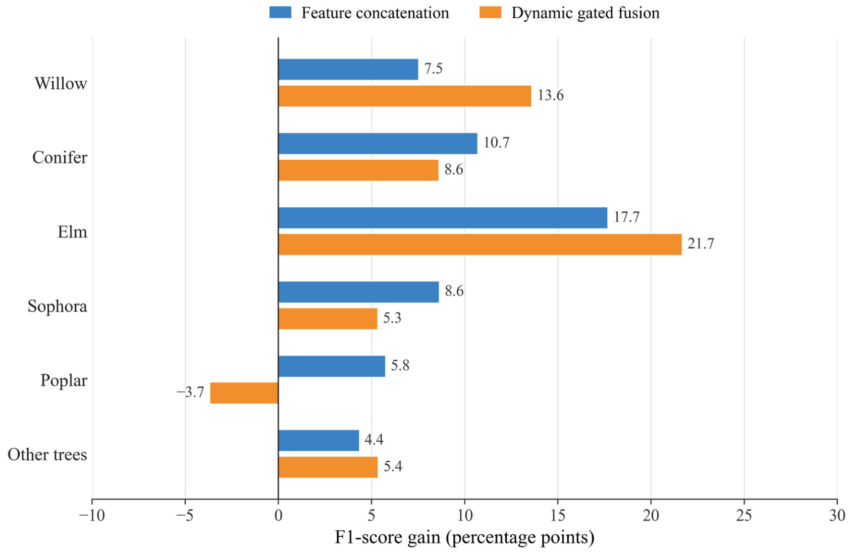
Species-specific F1 gains (Figure 14) provide further detail. Relative to input-level stacking, feature-level concatenation improved all six tree species classes, with F1 gains of 17.7%, 10.7%, and 8.6% for Elm, Conifer, and Sophora, respectively. Separate branch encoding therefore better preserves discriminative information from each modality. Dynamic gated fusion produced especially large gains for Willow and Elm, increasing F1 by 13.6% and 21.7%, respectively, and also improved Other trees. Pixel- and channel-adaptive weights can thus alleviate local confusion among broadleaf species. Poplar F1 decreased by 3.7% relative to input-level stacking, suggesting that more complex fusion does not necessarily optimize every individual class when that class already has a readily distinguishable canopy structure in the original features.

5.1.3. Comparison of Hyperspectral–Semantic Prior Strategies

Using the dynamic gated model without HSI (Experiment 4) as the baseline, we compared different mechanisms for introducing hyperspectral–semantic priors to evaluate the reliability-aware HSI prior module (

Table 15. Comparison of hyperspectral prior fusion strategies.

HSI Fusion Strategy	Corresponding Exp.	OA/%	Tree OA/%	mIoU/%	Macro-F1/%
No-HSI dynamic-fusion baseline	Exp. 4	89.25	81.90	71.95	82.94
Spatial bias prior	Exp. 9	89.52	81.71	75.88	85.51
Channel-modulation prior	Exp. 10	88.72	80.81	71.61	82.74
Class prior	Exp. 11	89.20	83.21	72.79	83.63
Fixed-reliability semantic prior	Exp. 12	89.71	82.35	73.95	84.55
Reliability-aware semantic prior	Exp. 6	90.44	85.06	77.88	87.15

). The spatial bias prior improved mIoU and Macro-F1 but yielded a slightly lower Tree OA than the no-HSI baseline. Although a coarse-scale spatial prior can enhance semantic representation in some areas, it may interfere with local crown boundaries. The class prior increased Tree OA to 83.21%, showing that class tendencies produced by the hyperspectral branch assist tree species discrimination. The fixed-reliability semantic prior outperformed the spatial bias and class prior configurations on some metrics but remained inferior to reliability-aware fusion [20,32,56].

The complete HybridFusion model with the reliability-aware semantic prior achieved the best performance, with Tree OA, mIoU, and Macro-F1 of 85.06%, 77.88%, and 87.15%, respectively. Relative to the no-HSI baseline, these values represent gains of 3.16% in Tree OA and 5.93% in mIoU. Hyperspectral information is therefore better used as a deep semantic complement that improves class discrimination than as a replacement for high-resolution spatial features in urban forest classification. Reliability gating regulates the strength of the HSI prior across samples, preserving high-resolution spatial representation while improving semantic separation among easily confused species.

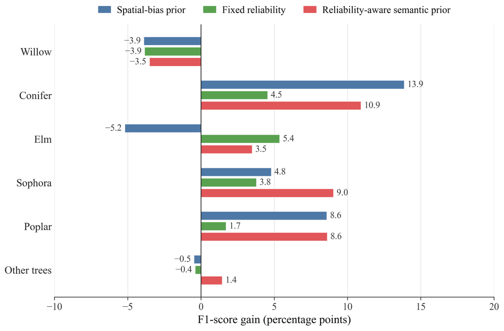
Species-specific F1 gains (Figure 15) show that the effect of the hyperspectral prior varies by class. Relative to the no-HSI dynamic-fusion baseline, the spatial bias prior increased F1 by 13.9% for Conifer and 8.6% for Poplar but decreased F1 for Willow, Elm, and Other trees. A coarse-scale spatial prior may therefore overcorrect mixed regions and local crown boundaries. The fixed-reliability semantic prior produced more stable gains of 5.4%, 4.5%, and 3.8% for Elm, Conifer, and Sophora, respectively, but had limited effects on Poplar and Other trees. In contrast, the reliability-aware semantic prior improved F1 by 10.9%, 9.0%, and 8.6% for Conifer, Sophora, and Poplar, respectively; it also maintained positive gains for Elm and Other trees, with only a slight decrease for Willow. Reliability gating therefore preserves the semantic contribution of hyperspectral data while reducing interference from low-resolution priors in classes defined by fine spatial detail, allowing HSI information to contribute more selectively to species discrimination.

5.1.4. Accuracy–Efficiency Trade-Off Among Full-Modality Architectures

The architecture-level comparison further clarifies the source of the performance improvement. FullModal-FPN achieved the highest accuracy among the conventional semantic segmentation baselines, demonstrating the importance of multiscale feature aggregation for heterogeneous urban tree crowns. Nevertheless, HybridFusion maintained advantages of 2.71 percentage points in Tree OA and 3.69 percentage points in mIoU over FullModal-FPN under the same full-modality setting. This improvement supports the contribution of reliability-aware hyperspectral–semantic guidance and dynamic multi-modal fusion beyond direct concatenation or conventional feature-pyramid processing. The efficiency analysis also reveals a clear accuracy–efficiency trade-off. HybridFusion is preferable when fine-grained classification accuracy is the primary objective, whereas FullModal-FPN provides a more balanced alternative under stricter memory and latency constraints, and MultiModal-Concat represents the lightest deployment-oriented baseline.

5.2. Sources of Classification Error and Uncertainty

Several factors contribute to the residual classification errors and the observed variation across spatially independent folds.

Class separability is limited because several tree species exhibit similar crown appearance and phenological responses. Willow, Elm, Sophora, and other broadleaf species in the study area may have similar growing-season crown color, texture, and spectral responses, which cannot always be fully separated using a single-date high-resolution image. Multi-temporal NDVI provides additional phenological information, but the March, April, and August observations mainly represent the transition from early spring to the growing season and do not fully capture leaf expansion, peak foliage, and senescence for all broadleaf species. Confusion therefore remains when different species exhibit similar greenness trajectories or vegetation-index values during the observation period.

These spectral and phenological ambiguities are further compounded by spatially heterogeneous forest structure [57]. The northern section of Olympic Forest Park contains pure stands, mixed conifer–broadleaf stands, forest-edge belts, riparian forests, and roadside green belts. Within these environments, a 2 m classification unit may contain contributions from multiple crowns, understory vegetation, background surfaces, or shadows. As a result, the pixel-level label may not always correspond to a single, clearly identifiable canopy. LiDAR features provide complementary information about tree height, canopy relief, and canopy closure, and they improve the recognition of Poplar and some tall trees. However, their discriminative contribution is reduced when different species have similar canopy heights or vertical structures.

The temporal relationship between the data sources may also introduce modality-specific inconsistencies [58]. The LiDAR structural features were acquired in 2022, whereas the main optical and hyperspectral observations were acquired in 2024–2025. The study area is a protected urban forest park without large-scale harvesting, and the macro-scale structure of mature trees was therefore expected to remain relatively stable. Nevertheless, localized crown growth, branch loss, pruning, storm damage, disease, mortality, and maintenance activities may have changed individual-tree height, crown extent, canopy closure, gap fraction, or leaf area index. Consequently, some LiDAR-derived features may not perfectly represent the canopy conditions observed in the later optical and hyperspectral data. Because these structural features guide the spatial branch in the dynamic fusion module, such discrepancies may lead to inconsistent multi-modal responses, particularly for small or rapidly changing trees and samples near canopy boundaries.

The spatially independent evaluation provides further evidence for assessing model generalization. Under the original validation protocol, HybridFusion achieved an OA of 90.44%, a Tree OA of 85.06%, a Kappa coefficient of 0.8707, an mIoU of 77.88%, and a Macro-F1 of 87.15%. Taking these development-validation results as the reference performance, the subsequent five-fold spatially independent evaluation yielded fold-to-fold variations of ±5.507% for OA, ±4.446% for Tree OA, ±0.075 for Kappa, ±5.354% for mIoU, and ±5.580% for Macro-F1. The observed variability indicates that model performance depends not only on the network architecture and input modalities but also on the geographic composition, species distribution, and structural complexity of the held-out areas. Tree species in Olympic Forest Park are spatially clustered rather than uniformly distributed. Consequently, different test folds contain different proportions of pure stands, mixed stands, riparian forests, roadside vegetation, and forest-edge communities, resulting in differences in classification difficulty. Future work should prioritize the collection of multi-modal datasets from new geographic regions and the construction of independently annotated test sets. Cross-region validation using these datasets would provide a more comprehensive assessment of the transferability and practical generalization capability of the proposed framework.

6. Conclusions

This study developed an advanced multi-source data fusion framework implemented in the northern section of Beijing’s Olympic Forest Park. By systematically integrating 0.5 m high-resolution imagery, multi-temporal NDVI, LiDAR structural metrics, and hyperspectral–semantic priors on a 2 m grid, comprehensive experiments, class-level assessments, and full-area mapping yielded the following key conclusions:

(1) Superior performance of multi-source data fusion. The full-modality integration achieved exceptional classification accuracy, with an OA of 90.44%, Tree OA of 85.06%, Kappa of 0.8707, mIoU of 77.88%, and Macro-F1 of 87.15%, substantially outperforming the single-source baseline. Poplar attained the highest F1 score (95.31%), followed by Willow (86.27%), Other trees (85.35%), and Conifer (84.90%).

(2) Phenological, canopy structural, and spectral–semantic data offer complementary contributions to tree species classification. Using high-resolution imagery alone, the overall accuracy (OA) was 67.29%. The addition of NDVI increased the OA to 76.06%. Incorporating LiDAR data raised the OA to 76.63%, indicating that metrics such as canopy height, relief, and closure effectively address the vertical spatial limitations of two-dimensional imagery. Furthermore, the joint application of NDVI and LiDAR boosted the OA to 81.90%. Finally, integrating a hyperspectral–semantic prior achieved a full-modality OA of 85.06%, highlighting that hyperspectral data serves as a powerful deep semantic complement to spatial texture, phenological, and structural features.

(3) Dynamic gated fusion and a reliability-aware hyperspectral prior improve multi-source fusion. High-resolution-side experiments showed that input-level stacking cannot adequately address differences in scale and noise among modalities, whereas dynamic gated fusion achieved the highest OA and Tree OA. LiDAR spatial modulation and joint pixel-channel gating therefore support adaptive allocation of modal contributions. Hyperspectral prior ablations showed that the reliability-aware semantic prior outperformed spatial bias, FiLM modulation alone, a class prior, and fixed reliability.

(4) Reliable large-scale mapping of urban forest structure. Study area-wide mapping revealed an effective mapping area of ~310.85 ha, with tree-covered zones accounting for ~175.12 ha (56.34%). Visual comparisons across representative scenes further corroborated that NDVI stabilizes conifer identification, LiDAR reinforces the spatial continuity of roadside tall-tree belts, and hyperspectral priors suppress local classification errors in complex mixed forests.

Several limitations should be acknowledged. First, the LiDAR observations were acquired in 2022, whereas the multispectral and hyperspectral data were collected during 2024–2025. Although no large-scale tree removal occurred in the protected study area, crown growth, pruning, branch loss, disease, storm damage, and routine maintenance may have altered local canopy structure, particularly in mixed stands and near crown boundaries. Second, the “Other trees” category combines multiple taxa with heterogeneous spectral, structural, and phenological characteristics, while the available samples may not represent each constituent species evenly. This limits class-specific interpretation and transferability to areas with different species compositions. Third, the full-modality HybridFusion model improves classification accuracy at the cost of increased computational complexity, memory usage, and inference time compared with simpler baseline models, which may constrain direct edge deployment. Future work should emphasize multi-site and multi-year validation, temporal calibration, and model-compression techniques.

References

1. Iungman, T.; Cirach, M.; Marando, F.; Barboza, E.P.; Khomenko, S.; Masselot, P.; Quijal-Zamorano, M.; Mueller, N.; Gasparrini, A.; Urquiza, J. Cooling cities through urban green infrastructure: A health impact assessment of European cities. Lancet 2023, 401, 577–589. [Google Scholar] [CrossRef] [Scilit] [PubMed]
2. Li, Y.; Svenning, J.-C.; Zhou, W.; Zhu, K.; Abrams, J.F.; Lenton, T.M.; Ripple, W.J.; Yu, Z.; Teng, S.N.; Dunn, R.R. Green spaces provide substantial but unequal urban cooling globally. Nat. Commun. 2024, 15, 7108. [Google Scholar] [CrossRef] [Scilit] [PubMed]
3. Livesley, S.; McPherson, E.G.; Calfapietra, C. The urban forest and ecosystem services: Impacts on urban water, heat, and pollution cycles at the tree, street, and city scale. J. Environ. Qual. 2016, 45, 119–124. [Google Scholar] [CrossRef] [Scilit] [PubMed]
4. Nowak, D.J.; Hirabayashi, S.; Bodine, A.; Greenfield, E. Tree and forest effects on air quality and human health in the United States. Environ. Pollut. 2014, 193, 119–129. [Google Scholar] [CrossRef] [Scilit] [PubMed]
5. Steenberg, J.W.; Ristow, M.; Duinker, P.N.; Lapointe-Elmrabti, L.; MacDonald, J.D.; Nowak, D.J.; Pasher, J.; Flemming, C.; Samson, C. A national assessment of urban forest carbon storage and sequestration in Canada. Carbon Balance Manag. 2023, 18, 11. [Google Scholar] [CrossRef] [Scilit] [PubMed]
6. Venter, Z.S.; Hassani, A.; Stange, E.; Schneider, P.; Castell, N. Reassessing the role of urban green space in air pollution control. Proc. Natl. Acad. Sci. USA 2024, 121, e2306200121. [Google Scholar] [CrossRef] [Scilit] [PubMed]
7. Zhao, X.; Jing, L.; Zhang, G.; Zhu, Z.; Liu, H.; Ren, S. Object-oriented convolutional neural network for forest stand classification based on multi-source data collaboration. Forests 2024, 15, 529. [Google Scholar] [CrossRef] [Scilit]
8. Cetin, Z.; Yastikli, N. The use of machine learning algorithms in urban tree species classification. ISPRS Int. J. Geo-Inf. 2022, 11, 226. [Google Scholar] [CrossRef] [Scilit]
9. Ocón, J.P.; Stavros, E.N.; Steinberg, S.J.; Robertson, J.; Gillespie, T.W. Remote sensing approaches to identify trees to species-level in the urban forest: A review. Prog. Phys. Geogr. Earth Environ. 2024, 48, 438–453. [Google Scholar] [CrossRef] [Scilit]
10. Tubby, K.; Webber, J. Pests and diseases threatening urban trees under a changing climate. Forestry 2010, 83, 451–459. [Google Scholar] [CrossRef] [Scilit]
11. Fassnacht, F.E.; White, J.C.; Wulder, M.A.; Næsset, E. Remote sensing in forestry: Current challenges, considerations and directions. For. Int. J. For. Res. 2024, 97, 11–37. [Google Scholar] [CrossRef] [Scilit]
12. He, X.; Ren, C.; Chen, L.; Wang, Z.; Zheng, H. The progress of forest ecosystems monitoring with remote sensing techniques. Geogr. Sci. 2018, 38, 997–1011. [Google Scholar] [CrossRef]
13. Fassnacht, F.E.; Latifi, H.; Stereńczak, K.; Modzelewska, A.; Lefsky, M.; Waser, L.T.; Straub, C.; Ghosh, A. Review of studies on tree species classification from remotely sensed data. Remote Sens. Environ. 2016, 186, 64–87. [Google Scholar] [CrossRef] [Scilit]
14. Liu, P.; Ren, C.; Wang, Z.; Jia, M.; Yu, W.; Ren, H.; Xia, C. Evaluating the potential of Sentinel-2 time series imagery and machine learning for tree species classification in a mountainous forest. Remote Sens. 2024, 16, 293. [Google Scholar] [CrossRef] [Scilit]
15. Beloiu, M.; Heinzmann, L.; Rehush, N.; Gessler, A.; Griess, V.C. Individual tree-crown detection and species identification in heterogeneous forests using aerial RGB imagery and deep learning. Remote Sens. 2023, 15, 1463. [Google Scholar] [CrossRef] [Scilit]
16. Deur, M.; Gašparović, M.; Balenović, I. Tree species classification in mixed deciduous forests using very high spatial resolution satellite imagery and machine learning methods. Remote Sens. 2020, 12, 3926. [Google Scholar] [CrossRef] [Scilit]
17. Neyns, R.; Canters, F. Mapping of urban vegetation with high-resolution remote sensing: A review. Remote Sens. 2022, 14, 1031. [Google Scholar] [CrossRef] [Scilit]
18. Ghamisi, P.; Yokoya, N.; Li, J.; Liao, W.; Liu, S.; Plaza, J.; Rasti, B.; Plaza, A. Advances in hyperspectral image and signal processing: A comprehensive overview of the state of the art. IEEE Geosci. Remote Sens. Mag. 2017, 5, 37–78. [Google Scholar] [CrossRef] [Scilit]
19. Gong, Y.; Zhu, D.e.; Li, X.; Lv, L.; Zhang, B.; Xuan, J.; Du, H. Using UAV LiDAR intensity frequency and hyperspectral features to improve the accuracy of urban tree species classification. IEEE J. Sel. Top. Appl. Earth Obs. Remote Sens. 2023, 17, 2849–2865. [Google Scholar] [CrossRef] [Scilit]
20. Ma, Y.; Zhao, Y.; Im, J.; Zhao, Y.; Zhen, Z. A deep-learning-based tree species classification for natural secondary forests using unmanned aerial vehicle hyperspectral images and LiDAR. Ecol. Indic. 2024, 159, 111608. [Google Scholar] [CrossRef] [Scilit]
21. Paoletti, M.E.; Haut, J.M.; Plaza, J.; Plaza, A. Deep learning classifiers for hyperspectral imaging: A review. ISPRS J. Photogramm. Remote Sens. 2019, 158, 279–317. [Google Scholar] [CrossRef] [Scilit]
22. Rasti, B.; Hong, D.; Hang, R.; Ghamisi, P.; Kang, X.; Chanussot, J.; Benediktsson, J.A. Feature extraction for hyperspectral imagery: The evolution from shallow to deep: Overview and toolbox. IEEE Geosci. Remote Sens. Mag. 2020, 8, 60–88. [Google Scholar] [CrossRef] [Scilit]
23. Cai, L.; Wu, D.; Fang, L.; Zheng, X. Tree species identification using XGBoost based on GF-2 images. For. Grassl. Resour. Res. 2019, 44–51. [Google Scholar] [CrossRef]
24. Li, Z.; Zhang, Q.-Y.; Qiu, X.-C.; Peng, D.-L. Temporal stage and method selection of tree species classification based on GF-2 remote sensing image. Ying Yong Sheng Tai Xue Bao J. Appl. Ecol. 2019, 30, 4059–4070. [Google Scholar] [CrossRef] [PubMed]
25. Cui, L.; Chen, S.; Mu, Y.; Xu, X.; Zhang, B.; Zhao, X. Tree species classification over cloudy mountainous regions by spatiotemporal fusion and ensemble classifier. Forests 2023, 14, 107. [Google Scholar] [CrossRef] [Scilit]
26. Ferreira, M.P.; dos Santos, D.R.; Ferrari, F.; Coelho, L.C.T.; Martins, G.B.; Feitosa, R.Q. Improving urban tree species classification by deep-learning based fusion of digital aerial images and LiDAR. Urban For. Urban Green. 2024, 94, 128240. [Google Scholar] [CrossRef] [Scilit]
27. Wang, L.; Lu, D.; Xu, L.; Robinson, D.T.; Tan, W.; Xie, Q.; Guan, H.; Chapman, M.A.; Li, J. Individual tree species classification using low-density airborne multispectral LiDAR data via attribute-aware cross-branch transformer. Remote Sens. Environ. 2024, 315, 114456. [Google Scholar] [CrossRef] [Scilit]
28. Hong, D.; Gao, L.; Yokoya, N.; Yao, J.; Chanussot, J.; Du, Q.; Zhang, B. More diverse means better: Multimodal deep learning meets remote-sensing imagery classification. IEEE Trans. Geosci. Remote Sens. 2020, 59, 4340–4354. [Google Scholar] [CrossRef] [Scilit]
29. Kattenborn, T.; Leitloff, J.; Schiefer, F.; Hinz, S. Review on Convolutional Neural Networks (CNN) in vegetation remote sensing. ISPRS J. Photogramm. Remote Sens. 2021, 173, 24–49. [Google Scholar] [CrossRef] [Scilit]
30. Hartling, S.; Sagan, V.; Maimaitijiang, M. Urban tree species classification using UAV-based multi-sensor data fusion and machine learning. GISci. Remote Sens. 2021, 58, 1250–1275. [Google Scholar] [CrossRef] [Scilit]
31. Sun, Y.; Xin, Q.; Huang, J.; Huang, B.; Zhang, H. Characterizing tree species of a tropical wetland in southern china at the individual tree level based on convolutional neural network. IEEE J. Sel. Top. Appl. Earth Obs. Remote Sens. 2019, 12, 4415–4425. [Google Scholar] [CrossRef] [Scilit]
32. Wu, J.; Chen, L.; Wang, J.; Li, Y.; Chen, E.; Zhang, X. A novel framework combining band selection algorithm and improved 3D prototypical network for tree species classification using airborne hyperspectral images. Comput. Electron. Agric. 2024, 219, 108813. [Google Scholar] [CrossRef] [Scilit]
33. Cao, Y.; Coops, N.C.; Murray, B.A.; Sinclair, I.; Geordie, R.-M. M3FNet: Multi-modal multi-temporal multi-scale data fusion network for tree species composition mapping. ISPRS J. Photogramm. Remote Sens. 2026, 231, 797–814. [Google Scholar] [CrossRef] [Scilit]
34. Ronneberger, O.; Fischer, P.; Brox, T. U-net: Convolutional networks for biomedical image segmentation. In Proceedings of the International Conference on Medical Image Computing and Computer-Assisted Intervention, Munich, Germany, 5–9 October 2015; pp. 234–241. [Google Scholar]
35. Liao, C.; Wang, J.; Xie, Q.; Baz, A.A.; Huang, X.; Shang, J.; He, Y. Synergistic use of multi-temporal RADARSAT-2 and VENµS data for crop classification based on 1D convolutional neural network. Remote Sens. 2020, 12, 832. [Google Scholar] [CrossRef] [Scilit]
36. Hartling, S.; Sagan, V.; Sidike, P.; Maimaitijiang, M.; Carron, J. Urban tree species classification using a WorldView-2/3 and LiDAR data fusion approach and deep learning. Sensors 2019, 19, 1284. [Google Scholar] [CrossRef] [Scilit] [PubMed]
37. Dersch, S.; Schöttl, A.; Krzystek, P.; Heurich, M. Semi-supervised multi-class tree crown delineation using aerial multispectral imagery and lidar data. ISPRS J. Photogramm. Remote Sens. 2024, 216, 154–167. [Google Scholar] [CrossRef] [Scilit]
38. Zhong, L.; Hu, L.; Zhou, H. Deep learning based multi-temporal crop classification. Remote Sens. Environ. 2019, 221, 430–443. [Google Scholar] [CrossRef] [Scilit]
39. Li, Z.; He, W.; Li, J.; Lu, F.; Zhang, H. Learning without exact guidance: Updating large-scale high-resolution land cover maps from low-resolution historical labels. In Proceedings of the 2024 IEEE/CVF Conference on Computer Vision and Pattern Recognition (CVPR), Seattle, WA, USA, 19–21 June 2024; pp. 27717–27727. [Google Scholar]
40. Huang, W.; Shi, Y.; Xiong, Z.; Zhu, X.X. Decouple and weight semi-supervised semantic segmentation of remote sensing images. ISPRS J. Photogramm. Remote Sens. 2024, 212, 13–26. [Google Scholar] [CrossRef] [Scilit]
41. Han, W.; Jiang, W.; Geng, J.; Miao, W. Difference-complementary learning and label reassignment for multimodal semi-supervised semantic segmentation of remote sensing images. IEEE Trans. Image Process. 2025, 34, 566–580. [Google Scholar] [CrossRef] [Scilit] [PubMed]
42. Ren, P.; Han, Z.; Yu, Z.; Zhang, B. Confucius tri-learning: A paradigm of learning from both good examples and bad examples. Pattern Recognit. 2025, 163, 111481. [Google Scholar] [CrossRef] [Scilit]
43. Han, Z.; Bai, L.; Pan, B.; Ren, P. From mutual guide to confucius tri-learning: A theoretical justification. Pattern Recognit. 2026, 178, 113447. [Google Scholar] [CrossRef] [Scilit]
44. Long, J.; Shelhamer, E.; Darrell, T. Fully convolutional networks for semantic segmentation. In Proceedings of the IEEE Conference on Computer Vision and Pattern Recognition, Boston, MA, USA, 7–12 June 2015; pp. 3431–3440. [Google Scholar]
45. He, K.; Zhang, X.; Ren, S.; Sun, J. Deep residual learning for image recognition. In Proceedings of the IEEE Conference on Computer Vision and Pattern Recognition, Las Vegas, NV, USA, 26 June–1 July 2016; pp. 770–778. [Google Scholar]
46. Chen, L.-C.; Papandreou, G.; Schroff, F.; Adam, H. Rethinking atrous convolution for semantic image segmentation. arXiv 2017, arXiv:1706.05587. [Google Scholar] [CrossRef] [Scilit]
47. Wu, H.; Wang, R.; Li, Y.; Bao, L. SC-LUFormer: A Scenario-Conditioned Transformer for Long-Term Land-Use Prediction from Remote Sensing Data in Mountainous Urban Agglomerations. IEEE J. Sel. Top. Appl. Earth Obs. Remote Sens. 2026, 19, 25001–25016. [Google Scholar] [CrossRef] [Scilit]
48. Hu, J.; Shen, L.; Sun, G. Squeeze-and-excitation networks. In Proceedings of the IEEE Conference on Computer Vision and Pattern Recognition, Salt Lake City, UT, USA, 18–22 June 2018; pp. 7132–7141. [Google Scholar]
49. Lin, T.-Y.; Dollár, P.; Girshick, R.; He, K.; Hariharan, B.; Belongie, S. Feature pyramid networks for object detection. In Proceedings of the IEEE Conference on Computer Vision and Pattern Recognition, Honolulu, HI, USA, 21–26 July 2017; pp. 2117–2125. [Google Scholar]
50. Xie, S.; Tu, Z. Holistically-nested edge detection. In Proceedings of the IEEE International Conference on Computer Vision, Santiago, Chile, 7–13 December 2015; pp. 1395–1403. [Google Scholar]
51. Alirr, O.I. A Large-Kernel and Scale-Aware 2D CNN with Boundary Refinement for Multimodal Ischemic Stroke Lesion Segmentation. Eng 2026, 7, 59. [Google Scholar] [CrossRef] [Scilit]
52. Loshchilov, I.; Hutter, F. Decoupled weight decay regularization. arXiv 2017, arXiv:1711.05101. [Google Scholar] [CrossRef] [Scilit]
53. Liang, X.; Chen, J.; Gong, W.; Puttonen, E.; Wang, Y. Influence of data and methods on high-resolution imagery-based tree species recognition considering phenology: The case of temperate forests. Remote Sens. Environ. 2025, 323, 114654. [Google Scholar] [CrossRef] [Scilit]
54. Neyns, R.; Efthymiadis, K.; Libin, P.; Canters, F. Fusion of multi-temporal PlanetScope data and very high-resolution aerial imagery for urban tree species mapping. Urban For. Urban Green. 2024, 99, 128410. [Google Scholar] [CrossRef] [Scilit]
55. Jiang, Y.; Li, X.; Peng, L.; Li, C.; Song, T. Assessing the potential of multi-seasonal Sentinel-2 satellite imagery combined with airborne LiDAR for urban tree species identification. Sci. Rep. 2025, 15, 25107. [Google Scholar] [CrossRef] [Scilit] [PubMed]
56. Wang, A.; Shi, S.; Yang, J.; Luo, Y.; Tang, X.; Du, J.; Bi, S.; Qu, F.; Gong, C.; Gong, W. Integration of lidar and hyperspectral imagery for tree species identification at the individual tree level. Photogramm. Rec. 2025, 40, e70007. [Google Scholar] [CrossRef] [Scilit]
57. Zhong, H.; Zhang, Z.; Liu, H.; Wu, J.; Lin, W. Individual tree species identification for complex coniferous and broad-leaved mixed forests based on deep learning combined with UAV LiDAR data and RGB images. Forests 2024, 15, 293. [Google Scholar] [CrossRef] [Scilit]
58. Han, Z.; Zhang, C.; Gao, L.; Zeng, Z.; Ng, M.K.; Zhang, B.; Chanussot, J. Multisource Collaborative Domain Generalization for Cross-Scene Remote Sensing Image Classification. IEEE Trans. Geosci. Remote Sens. 2024, 62, 5535815. [Google Scholar] [CrossRef] [Scilit]
Figure 1. Imagery of the study area and distribution of ground survey tree species samples.
Remotesensing 18 03246 g001
Figure 2. Overview of the multi-source remote sensing data.
Remotesensing 18 03246 g002
Figure 3. Workflow for multi-source remote sensing tree species classification.
Remotesensing 18 03246 g003
Figure 4. Multi-modal feature encoding module.
Remotesensing 18 03246 g004
Figure 5. Dynamic gated fusion module.
Remotesensing 18 03246 g005
Figure 6. Reliability-aware hyperspectral prior fusion module.
Remotesensing 18 03246 g006
Figure 7. Multiscale decoder module.
Remotesensing 18 03246 g007
Figure 8. t-SNE visualization of the original feature space: (a) high-resolution optical imagery only; (b) high-resolution imagery + multi-temporal NDVI; (c) high-resolution imagery + LiDAR structural features; (d) high-resolution imagery + NDVI + LiDAR.
Remotesensing 18 03246 g008
Figure 9. Heat map of class-mean LiDAR structural features.
Remotesensing 18 03246 g009
Figure 10. t-SNE visualization of deep fused features learned by the model, panels (a–f) correspond sequentially to Experiments 1–6.
Remotesensing 18 03246 g010
Figure 11. Tree species classification maps from the 12 experiments, panels (a–l) corresponding sequentially to Experiments 1–12.
Remotesensing 18 03246 g011
Figure 12. Tree species classification map produced by the full-modality HybridFusion model (corresponding to Exp 6).
Remotesensing 18 03246 g012
Figure 13. Local classification-detail comparison under different data source combinations.
Remotesensing 18 03246 g013
Figure 14. Species-specific F1 gains under different high-resolution-side fusion strategies.
Remotesensing 18 03246 g014
Figure 15. Species-specific F1 gains under different hyperspectral-side fusion strategies.
Remotesensing 18 03246 g015